h fl: computation and communication e f learning for

Published as a conference paper at ICLR 2021

HETEROFL: COMPUTATION AND COMMUNICATIONEFFICIENT FEDERATED LEARNING FOR HETEROGE-NEOUS CLIENTS

Enmao DiaoDepartment of Electrical and Computer EngineeringDuke UniversityDurhm, NC 27705, [email protected]

Jie DingSchool of StatisticsUniversity of Minnesota-Twin CitiesMinneapolis, MN 55455, [email protected]

Vahid TarokhDepartment of Electrical and Computer EngineeringDuke UniversityDurhm, NC 27705, [email protected]

ABSTRACT

Federated Learning (FL) is a method of training machine learning models on pri-vate data distributed over a large number of possibly heterogeneous clients suchas mobile phones and IoT devices. In this work, we propose a new federatedlearning framework named HeteroFL to address heterogeneous clients equippedwith very different computation and communication capabilities. Our solution canenable the training of heterogeneous local models with varying computation com-plexities and still produce a single global inference model. For the first time, ourmethod challenges the underlying assumption of existing work that local modelshave to share the same architecture as the global model. We demonstrate severalstrategies to enhance FL training and conduct extensive empirical evaluations, in-cluding five computation complexity levels of three model architecture on threedatasets. We show that adaptively distributing subnetworks according to clients’capabilities is both computation and communication efficient.

1 INTRODUCTION

Mobile devices and the Internet of Things (IoT) devices are becoming the primary computing re-source for billions of users worldwide (Lim et al., 2020). These devices generate a significantamount of data that can be used to improve numerous existing applications (Hard et al., 2018).From the privacy and economic point of view, due to these devices’ growing computational capa-bilities, it becomes increasingly attractive to store data and train models locally. Federated learning(FL) (Konecny et al., 2016; McMahan et al., 2017) is a distributed machine learning framework thatenables a number of clients to produce a global inference model without sharing local data by aggre-gating locally trained model parameters. A widely accepted assumption is that local models have toshare the same architecture as the global model (Li et al., 2020b) to produce a single global inferencemodel. With this underlying assumption, we have to limit the global model complexity for the mostindigent client to train its data. In practice, the computation and communication capabilities of eachclient may vary significantly and even dynamically. It is crucial to address heterogeneous clientsequipped with very different computation and communication capabilities.

In this work, we propose a new federated learning framework called HeteroFL to train heteroge-neous local models with varying computation complexities and still produce a single global infer-ence model. This model heterogeneity differs significantly from the classical distributed machinelearning framework where local data are trained with the same model architecture (Li et al., 2020b;Ben-Nun & Hoefler, 2019). It is natural to adaptively distribute subnetworks according to clients’

1


capabilities. However, to stably aggregate heterogeneous local models to a single global model un-der various heterogeneous settings is not apparent. Addressing these issues is thus a key componentof our work. Our main contributions of this work are three-fold.

• We identify the possibility of model heterogeneity and propose an easy-to-implementframework HeteroFL that can train heterogeneous local models and aggregate them stablyand effectively into a single global inference model. Our approach outperforms state-of-the-art results without introducing additional computation overhead.

• Our proposed solution addresses various heterogeneous settings where different propor-tions of clients have distinct capabilities. Our results demonstrate that even when the modelheterogeneity changes dynamically, the learning result from our framework is still stableand effective.

• We introduce several strategies for improving FL training and demonstrate that our methodis robust against the balanced non-IID statistical heterogeneity. Also, the proposed methodcan reduce the number of communication rounds needed to obtain state-of-the-art results.Experimental studies have been performed to evaluate the proposed approach.

2 RELATED WORK

Federated Learning aims to train massively distributed models at a large scale (Bonawitz et al.,2019). FedAvg proposed by McMahan et al. (2017) is currently the most widely adopted FL base-line, which reduces communication cost by allowing clients to train multiple iterations locally. Ma-jor challenges involved in FL include communication efficiency, system heterogeneity, statisticalheterogeneity, and privacy (Li et al., 2020b). To reduce communication costs in FL, some studiespropose to use data compression techniques such as quantization and sketching (Konecny et al.,2016; Alistarh et al., 2017; Ivkin et al., 2019), and some propose to adopt split learning (Thapaet al., 2020). To tackle system heterogeneity, techniques of asynchronous communication and activesampling of clients have been developed (Bonawitz et al., 2019; Nishio & Yonetani, 2019). Statis-tical heterogeneity is the major battleground for current FL research. A research trend is to adaptthe global model to accommodate personalized local models for non-IID data (Liang et al., 2020),e.g., by integrating FL with other frameworks such as assisted learning (Xian et al., 2020), meta-learning (Jiang et al., 2019; Khodak et al., 2019), multi-task learning (Smith et al., 2017), transferlearning (Wang et al., 2019; Mansour et al., 2020), knowledge distillation (Li & Wang, 2019) andlottery ticket hypothesis (Li et al., 2020a). Nevertheless, these personalization methods often in-troduce additional computation and communication overhead that may not be necessary. Anothermajor concern of FL is data privacy (Lyu et al., 2020), as model gradient updates can reveal sensitiveinformation (Melis et al., 2019) and even local training data (Zhu et al., 2019; Zhao et al., 2020).

To our best knowledge, what we present is the first work that allows local models to have different ar-chitectures from the global model. Heterogeneous local models can allow local clients to adaptivelycontribute to the training of global models. System heterogeneity and communication efficiencycan be well addressed by our approach, where local clients can optimize low computation complex-ity models and therefore communicate a small number of model parameters. To address statisticalheterogeneity, we propose a ”Masking Trick” for balanced non-IID data partition in classificationproblems. We also propose a modification of Batch Normalization (BN) (Ioffe & Szegedy, 2015) asprivacy concern of running estimates hinders the usage of advanced deep learning models.

3 HETEROGENEOUS FEDERATED LEARNING

3.1 HETEROGENEOUS MODELS

Federated Learning aims to train a global inference model from locally distributed data{X1, . . . , Xm} across m clients. The local models are parameterized by model parameters{W1, . . . ,Wm}. The server will receive local model parameters and aggregate them into a globalmodel Wg through model averaging. This process iterates multiple communication rounds and canbe formulated as W t

g = 1m

∑mi=1W

ti at iteration t. At the next iteration, W t

g is transmitted to asubset of local clients and update their local models as W t+1

i =W tg .

2


Local model parameters



Global model parameters

Figure 1: Global model parameters Wg are distributed to m = 6 local clients with p = 3 computa-tion complexity levels.

In this work, we focus on the relaxation of the assumption that local models need to share the samearchitecture as the global model. Since our primary motivation is to reduce the computation andcommunication complexity of local clients, we consider local models to have similar architecturebut can shrink their complexity within the same model class. To simplify global aggregation andlocal update, it is tempting to propose local model parameters to be a subset of global model pa-rameters W t+1

i ⊆ W tg . However, this raises several new challenges like the optimal way to select

subsets of global model parameters, compatibility of the-state-of-art model architecture, and mini-mum modification from the existing FL framework. We develop Heterogeneous Federated Learning(HeteroFL) to address these issues in the context of deep learning models.

A variety of works show that we can modulate the size of deep neural networks by varying the widthand depth of networks (Zagoruyko & Komodakis, 2016; Tan & Le, 2019). Because we aim to reducethe computation complexity of local models, we choose to vary the width of hidden channels. In thisway, we can significantly reduce the number of local model parameters, while the local and globalmodel architectures are also within the same model class, which stabilizes global model aggregation.

We demonstrate our method of selecting subsets of global model parameters Wl for a single hiddenlayer parameterized by Wg ∈ Rdg×kg in Fig. 1, where dg and kg are the output and input channelsize of this layer. It is possible to have multiple computation complexity levels W p

l ⊂ W p−1l · · · ⊂

W 1l as illustrated in Fig. 1. Let r be the hidden channel shrinkage ratio such that dpl = rp−1dg and

kpl = rp−1kg . It follows that the size of local model parameters |W pl | = r2(p−1)|Wg| and the model

shrinkage ratio R =|Wp

l ||Wg| = r2(p−1). With this construction, we can adaptively allocate subsets of

global model parameters according to the corresponding capabilities of local clients. Suppose thatnumber of clients in each computation complexity level is {m1, . . . ,mp}. Specifically, we performglobal aggregation in the following way.

W pl =

1

m

m∑i=1

W pi , W p−1

l \W pl =

1

m−mp

m−mp∑i=1

W p−1i \W p

i , . . . (1)

W 1l \W 2

l =1

m−m2:p

m−m2:p∑i=1

W 1i \W 2

i (2)

Wg =W 1l =W p

l ∪ (W p−1l \W p

l ) ∪ · · · ∪ (W 1l \W 2

l ) (3)

For notational convenience, we have dropped the iteration index t. We denote the W pi as a ma-

trix/tensor. The W tg [: dm, : km] denotes the upper left submatrix with a size of dm × km. Also,

W p−1,t+1g \W p,t+1

g denotes the set of elements included in W p−1,t+1g but excluded in W p,t+1

g .

We exemplify the above equations using Fig. 1. The first part of Equation (1) shows that the smallestpart of model parameters (blue, p = 3) is aggregated from all the local clients that contain it.

3


In the second part of Equation (1), the set difference between part p − 1 (orange) and p (blue)of model parameters is aggregated from local clients with computation complexity level smallerthan p − 1. In Equation (2), the red part of model parameters can be similarly aggregated fromm −m2:p = m1 clients. In Equation (3), the global model parameters W t

g is constructed from theunion of all disjoint sets of the partition. In summary, each parameter will be averaged from thoseclients whose allocated parameter matrix contains that parameter. Thus, a model of an intermediatecomplexity will have parameters fully averaged with all the other larger models but partially withsmaller models (according to the corresponding upper left submatrix).

Several works show that wide neural networks can drop a tremendous number of parameters perlayer and still produce acceptable results (Han et al., 2015; Frankle & Carbin, 2018). The intuition isthus to perform global aggregation across all local models, at least on one subnetwork. To stabilizeglobal model aggregation, we also allocate a fixed subnetwork for every computation complexitylevel. Our proposed inclusive subsets of global model parameters also guarantee that smaller localmodels will aggregate with more local models.

Thus, small local models can benefit more from global aggregation by performing less global aggre-gation for part of larger local model parameters. We empirically found that this approach producesbetter results than uniformly sampled subnetworks for each client or computation complexity level.

3.2 STATIC BATCH NORMALIZATION

After global model parameters are distributed to active local clients, we can optimize local model pa-rameters with private data. It is well-known that the latest deep learning models usually adopt BatchNormalization (BN) to facilitate and stabilize optimization. However, classical FedAvg and mostrecent works avoid BN. A major concern of BN is that it requires running estimates of representa-tions at every hidden layer. Uploading these statistics to the server will cause higher communicationcosts and privacy issues Andreux et al. (2020) proposes to track running statistics locally.

We highlight an adaptation of BN named as static Batch Normaliztion (sBN) for optimizing pri-vacy constrained heterogeneous models. During the training phase, sBN does not track runningestimates and simply normalize batch data. We do not track the local running statistics as the size oflocal models may also vary dynamically. This method is suitable for HeteroFL as every communi-cation round is independent. After the training process finishes, the server sequentially query localclients and cumulatively update global BN statistics. There exist privacy concerns about calculatingglobal statistics cumulatively and we hope to address those issues in the future work. We also em-pirically found this trick significantly outperforms other forms of normalization methods includingthe InstanceNorm (Ulyanov et al., 2016), GroupNorm (Wu & He, 2018), and LayerNorm (Ba et al.,2016) as shown in Table 4 and Table 5.

3.3 SCALER

There still exists another cornerstone of our HeteroFL framework. Because we need to optimizelocal models for multiple epochs, local model parameters at different computation complexity lev-els will digress to various scales. This known phenomenon was initially discussed by the dropout(Srivastava et al., 2014). To directly use the full model during the inference phase, inverted dropoutwith dropout rate q scales representations with 1

1−q during the training phase. In practice, dropout isusually attached after the activation layer as the selection of subnetworks is performed with masking.Our method directly selects subnetworks from the subsets of global model parameters. Therefore,we append a Scaler module right after the parametric layer and before the sBN and activation layers.The Scaler module scales representations by 1

rp−1 during the training phase. After the global aggre-gation, the global model can be directly used for inference without scaling. To further illustrate thispoint, we include a comprehensive ablation study in Tables 4 and 5. A typical linear hidden layerused in our HeteroFL framework can be formulated as

y = φ(sBN(Scaler(XmWpm + bpm))) (4)

where y is the output, φ(·) denotes a non-linear activation layer, e.g ReLU(), and W pm, b

pm are the

weight and bias for local model m at computation complexity level p. With all the practical meth-ods mentioned above, we propose the complete pseudo-code for our HeteroFL framework in Algo-rithm 1. The local capabilities information Lm is an abstraction of the computation and communica-

4


Algorithm 1: HeteroFL: Heterogeneous Federated LearningInput: Data Xi distributed on M local clients, the fraction C of active clients per

communication round, the number of local epochs E, the local minibatch size B, thelearning rate η, the global model parameterized by Wg , the channel shrinkage ratio r,and the number of computation complexity levels P .

System executes:Initialize W 0

g and local capabilities information L1:K

for each communication round t = 0, 1, 2, . . . doMt ← max(C ·M, 1)St ← random set of Mt clientsfor each client m ∈ St in parallel do

Determine computation complexity level p based on Lm

rm ← r(p−1), dm ← rmdg , km ← rmkgW t

m ←W tg [: dm, : km]

W t+1m ← ClientUpdate(m, rm,W t

m)endfor each computation complexity level p do

W p−1,t+1g \W p,t+1

g ← 1Mt−Mp:P,t

∑Mt−Mp:P,t

i=1 W p−1,t+1i \W p,t+1

i

endW t+1

g ←⋃P

p=1Wp−1,t+1g \W p,t+1

g

Update L1:K , η (Optional)endQuery representation statistics from local clients (Optional)

ClientUpdate (m, rm,Wm):Bm ← Split local data Xm into batches of size Bfor each local epoch e from 1 to E do

for batch bm ∈ Bm doWm ←Wm − η∇`(Wm, rm; bm)

endendReturn Wm to server

tion capabilities of a local client m. Once this information is communicated to the server, the servercan know the model complexity that should be allocated to the client. We can also optionally updatelearning rates to facilitate optimization and local capabilities information if changing dynamically.

4 EXPERIMENTAL RESULTS

We trained over 600 individual models for exploring and demonstrating the effectiveness of ourmethod. We experimented with MNIST and CIFAR10 image classification tasks and the WikiText2language modeling task (LeCun et al., 1998; Krizhevsky et al., 2009; Merity et al., 2016; Devlinet al., 2018).

Our experiments are performed with three different models including a CNN for MNIST, a preacti-vated ResNet (PreResNet18) (He et al., 2016) for CIFAR10 and a Transformer (Vaswani et al., 2017)for WikiText2. We replace BN in CNN and PreResNet18 with our proposed sBN, and attach theScaler module after each convolution layer. To study federated optimization, we adopt data partitionthe same as in (McMahan et al., 2017; Liang et al., 2020). We have 100 clients, and the fraction Cof active clients per communication round is 0.1 throughout our experiments. For IID data partition,we uniformly assign the same number of data examples for each client. For balanced non-IID datapartition, we assume that the label distribution is skewed, where clients will only have examples atmost from two classes and the number of examples per class is balanced. We note that there existother kinds of non-IID data partition, e.g., the unbalanced non-IID data partition where clients mayhold unbalanced labeled dataset and the feature distribution skew where clients may hold differentfeatures. We conduct a masked language modeling task with a 15% masking rate and uniformly

5


assign balanced data examples for each client. It needs to point out that each client will roughlyhave 3000 different words in their local dataset, while the total vocabulary size is 33278. The detailsregarding hyperparameters and model architecture can be found in Table 6 of the Appendix.

To study the effectiveness of our proposed HeteroFL framework, we construct five different com-putation complexity levels {a, b, c, d, e} with the hidden channel shrinkage ratio r = 0.5. We havetried various shrinkage ratios, and we found that it is most illustrative to use the discrete complexitylevels 0.5, 0.25, 0.125, and 0.0625 (relative to the most complex model). For example, model ‘a’ hasall the model parameters, while models ‘b’ to ‘e’ have the effective shrinkage ratios 0.5, 0.25, 0.125,and 0.0625. We note that the complexity of ‘e’ is close to a logistic regression model. Our experi-ments indicated that the ratio can be arbitrary between (0, 1] and dynamically change. In practice,using a dictionary of discrete complexity levels are convenient for coordination purposes.

Each local client is assigned an initial computation complexity level. We annotate Fix for exper-iments with a fixed assignment of computation complexity levels, and Dynamic for local clientsuniformly sampling computation complexity levels at each communication round. We perform dis-tinct experiments for Fix and Dynamic assignments. All the figures are based on the Fix scenario,where we considered models of different sizes, and each client is allocated with a fixed size. All thetables are based on the Dynamic scenario, where we randomly vary the allocation of clients’ modelcomplexity, and the ratio of the number of weak learners is fixed to 50%.

The x-axis of figures represents the average model parameters. When 10% clients use the model ’a’and 90% use the model ’e’, the average number of model parameters is 0.1× (size of model ‘a’) +0.9 × (size of model ‘e’). We interpolate this partition from 10% to 100% with step size 10% todemonstrate the effect of proportionality of clients with various computation complexity levels.

To demonstrate the effect of dynamically varying computation and communication capabilities, weuniformly sample from various combinations of computation complexity levels. For example, model’a-b-c-d-e’ means that we uniformly sample from all possible available levels for every active clientat each communication round. We show the number of model parameters, FLOPs, and Space (MB)to indicate the computation and communication requirements of our methods. For example, sincewe uniformly sample levels, model a − e calculates computational metrics by averaging those ofmodel a and e. The ratio is calculated between the number of parameters of a given model withrespect to its 100% global model.

We compare our results to other baseline methods like Standalone, FedAvg, and LG-FedAvg gath-ered from (Liang et al., 2020). Standalone means there is no communication between clients andthe server. In our experimental studies, we considered more complex models compared with theexisting work. In particular, the baseline models in LG-FedAvg used MLP (on MNIST) and CNN(on CIFAR10). In terms of the number of parameters, our models ‘a-e’ (on MNIST) and ‘b-e’(on CIFAR10) are comparable with those baselines. In terms of the FLOPs, our model ‘d-e’ (onMNIST and CIFAR10) can be compared with those baselines. The single-letter models ‘a’, ‘b’,‘c’, ‘d’, ‘e’ are our implementations of the FedAvg equipped with the sBN and Masking CrossEn-tropy. The takeaway of Table 2 is that a weak learner that can only train a small model ‘e’ (onCIFAR10)(77.09%) can boost its performance to ‘c-e’ (86.88%), ‘b-e’ (89.10%), or ‘a-e’ (90.29%),which are close to the scenario where all the learners are strong, namely c(87.55%), b(89.82%), ora(91.99%). In particular, in ‘c-e’, ‘b-e’, or ‘a-e’, half of the clients are trained with larger models ‘c’,‘b’, or ‘a’, while the other half are trained with the model ‘e’. Only the aggregated global models‘c’, ‘b’, or ‘a’ are used during the testing stage. Although weak clients train smaller models ‘e’, theywill test with the largest models ‘c’, ‘b’, or ‘a’ to gain better performance.

Full results including other possible combinations can be found in appendix in Table 7-9. Finally, ourmethod is robust to dynamically varying model complexities. It is worth noting that our method doesnot incur any additional computation overhead and can be readily adapted to existing applications.

We also perform experiments for balanced non-IID data partition and provide a simple trick toachieve comparable results. As mentioned earlier, most state-of-the-art results ofbalanced non-IIDdatasets suggest the personalization of local models to achieve better local results (Smith et al., 2017;Liang et al., 2020; Li et al., 2020a). Here, the Local results assume that the training data distributionand test data distribution for each local client are the same, and assign zero probability for thoseclasses that are not presented to a client during training. The Global results were calculated from theglobal model applied to the test data directly. The Local results were cumulatively averaged from

6


(a) (b)

(c) (d)

Figure 2: Interpolation experimental results for CIFAR10 (IID) dataset between global model com-plexity ((a) a, (b) b, (c) c, (d) d) and various smaller model complexities.

the performance of each data example on each local client. Zhao et al. (2018) showed that the failureof non-IID FL is related to the weight divergence among local model parameters trained locally formany iterations. The weight divergence mostly occurs in the last classification layer of networks.

Thus, instead of a full Cross-Entropy Loss for all classes, we are motivated to train each local modelonly with their corresponding classes. In this way, each local model will train a sub-task given lo-cally available label information. Specifically, we mask out the output of the model before passingit Cross-Entropy Loss, which we named as Masked Cross-Entropy Loss. We experimented withseveral different ways of masking, we find replacing the last layer outputs that are not associatedwith local labels with zero achieves both stable and comparable local and global results. Whenaggregating local model parameters, we do not aggregate the untrained parameters in the last classi-fication layers. Either the server can infer this information implicitly, or the local clients can reportwhich classes they have to the server explicitly. We provide a comprehensive ablation study in Ta-bles 5. The results show that Masked Cross-Entropy Loss significantly improve local performanceand moderately global performance of balanced non-IID data partition task. Since our primary focusis to address model heterogeneity, we leave the analysis of this trick to future work. We show theresults of Fix experiments in appendix in Fig. 5-8. Dynamic non-IID results are also included inTable 1-3. The results show that our method performs comparably to those with personalized localmodels. Our method is readily adaptable, free of computation overhead, and only rely on the singleglobal model for testing local and global results. It allows local clients to switch to another subtasksimply by changing its mask without querying the server for others’ personalized models.

We show the learning curves of 50% Fix and Dynamic assignments in appendix in Fig. 9-11. Thelearning curves show that the optimization of HeteroFL for the IID dataset is stable and efficient.Our method achieves better results with a fewer number of communication rounds, e.g., 800 forHeterofl and 1800 for LG-FedAvg (Liang et al., 2020). We empirically discover gradient clippingstabilizes the optimization of HeteroFL as it prevents small models from gradient explosion. Wecan therefore adopt a universal learning rate for heterogeneous local models. It is also perceivable

7


Model Ratio Parameters FLOPs Space (MB)Accuracy

IID Non-IID

Local Global

a 1.00 1.6 M 80.5 M 5.94 99.53 99.85 98.92a-e 0.50 782 K 40.5 M 2.98 99.46 99.89 98.96

a-b-c-d-e 0.27 416 K 21.6 M 1.59 99.46 99.85 98.29

b 1.00 391 K 20.5 M 1.49 99.53 99.87 99.10b-e 0.51 199 K 10.4 M 0.76 99.51 99.67 98.51

b-c-d-e 0.33 131 K 6.9 M 0.50 99.52 99.88 98.99

c 1.00 99 K 5.3 M 0.38 99.35 99.56 96.34c-e 0.53 53 K 2.9 M 0.20 99.39 99.79 97.27

c-d-e 0.44 44 K 2.4 M 0.17 99.31 99.76 97.85

d 1.00 25 K 1.4 M 0.10 99.17 99.86 97.86d-e 0.63 16 K 909 K 0.06 99.19 99.63 97.70

e 1.00 7 K 400 K 0.03 98.66 99.07 92.84

Standalone (Liang et al., 2020) 1.00 633 K 1.3 M 2.42 86.24 98.72 30.41FedAvg (Liang et al., 2020) 1.00 633 K 1.3 M 2.42 97.93 98.20 98.20

LG-FedAvg (Liang et al., 2020) 1.00 633 K 1.3 M 2.42 97.93 98.54 98.17

Table 1: Results of combination of various computation complexity levels for MNIST dataset. Fullresults can be found in Table 7.


IID Non-IID

Local Global

a 1.00 9.6 M 330.2 M 36.71 91.19 92.38 56.88a-e 0.50 4.8 M 165.9 M 18.43 90.29 92.10 59.11

a-b-c-d-e 0.27 2.6 M 88.4 M 9.78 88.83 92.49 61.64

b 1.00 2.4 M 83.3 M 9.19 89.82 93.83 55.45b-e 0.51 1.2 M 42.4 M 4.67 89.10 90.68 59.81

b-c-d-e 0.33 801 K 27.9 M 3.05 87.92 91.90 59.10

c 1.00 604 K 21.2 M 2.30 87.55 91.09 55.12c-e 0.53 321 K 11.3 M 1.22 86.88 91.83 63.47

c-d-e 0.44 265 K 9.4 M 1.01 85.79 91.49 55.42

d 1.00 152 K 5.5 M 0.58 84.21 90.77 61.13d-e 0.63 95 K 3.5 M 0.36 82.93 90.89 56.16

e 1.00 38 K 1.5 M 0.15 77.09 89.62 54.16

Standalone (Liang et al., 2020) 1.00 1.8 M 3.6 M 6.88 16.90 87.93 10.03FedAvg (Liang et al., 2020) 1.00 1.8 M 3.6 M 6.88 67.74 58.99 58.99

LG-FedAvg (Liang et al., 2020) 1.00 1.8 M 3.6 M 6.88 69.76 91.77 60.79

Table 2: Results of combination of various computation complexity levels for CIFAR10 dataset.Full results can be found in Table 8.

that aggregation of model parameters trained with non-IID data makes the optimization less stable.Results of Dynamic show that global aggregation of dynamically varying computation complexitiesis stable.

5 CONCLUSIONS AND FUTURE WORK

We propose Heterogeneous Federated Learning (HeteroFL), which shows the possibility of coordi-natively training local models much smaller than a global model to produce a single global infer-ence model. Our experiments show that FL can be made more practical by introducing HeteroFL

8


Model Ratio Parameters FLOPs Space (MB) Perplexity

a 1.00 19.3 M 1.4 B 73.49 3.37a-e 0.53 10.2 M 718.6 M 38.86 3.75

a-b-c-d-e 0.37 7.2 M 496.6 M 27.55 3.55

b 1.00 9.1 M 614.8 M 34.74 3.46b-e 0.56 5.1 M 342.0 M 19.49 3.90

b-c-d-e 0.46 4.2 M 278.7 M 16.07 3.64

c 1.00 4.4 M 290.1 M 16.92 3.62c-e 0.62 2.8 M 179.7 M 10.57 3.89

c-d-e 0.58 2.6 M 166.7 M 9.85 3.66

d 1.00 2.2 M 140.7 M 8.39 3.83d-e 0.75 1.7 M 105.0 M 6.31 3.90

e 1.00 1.1 M 69.3 M 4.23 7.41

Table 3: Results of combination of various computation complexity levels for WikiText2 dataset.Full results can be found in Table 9.

Model Normalization Scaler Accuracy IID

MNIST CIFAR10

a

None

N/A

99.2 81.3IN 99.5 87.7GN 99.5 81.0LN 99.5 77.3sBN 99.6 91.7

e

None

N/A

98.6 58.1IN 97.4 66.4GN 98.7 62.6LN 98.6 53.7sBN 98.7 77.0

a-e

None7

99.5 80.1sBN 99.0 90.1

None

3

99.2 80.4IN 99.5 86.6GN 99.5 76.0LN 99.4 71.7sBN 99.5 90.1

Table 4: Ablation Study of IID scenarios. The single-letter models ’a’ and ’e’ are FedAvg equipedwith various normalization methods. The sBN significantly outperforms other existing normaliza-tion methods, including the InstanceNorm (IN), GroupNorm (GN) (the number of group G=4), andLayerNorm (LN). Scaler is used for HeteroFL to train models of different sizes and moderatelyimprove the results.

and sBN and Mased Cross-Entropy Loss, as HeteroFL fully exploits local clients’ capabilities andachieves better results with a fewer number of communication rounds. We demonstrate our resultswith various model architectures, including CNN, PreResNet18, and Transformer, and show thatour method is robust to statistical heterogeneity and dynamically varying local capabilities. A futuredirection is to distinct model classes as well as model heterogeneity. Also, the proposed methodsmay be emulated to address heterogeneous few-shot learning, multi-modal learning, and multi-tasklearning.

ACKNOWLEDGMENTS

This work was supported by the Office of Naval Research (ONR) under grant number N00014-18-1-2244, and the Army Research Office (ARO) under grant number W911NF-20-1-0222.

9


REFERENCES

Dan Alistarh, Demjan Grubic, Jerry Li, Ryota Tomioka, and Milan Vojnovic. Qsgd:Communication-efficient sgd via gradient quantization and encoding. In Advances in NeuralInformation Processing Systems, pp. 1709–1720, 2017.

Mathieu Andreux, Jean Ogier du Terrail, Constance Beguier, and Eric W Tramel. Siloed federatedlearning for multi-centric histopathology datasets. In Domain Adaptation and RepresentationTransfer, and Distributed and Collaborative Learning, pp. 129–139. Springer, 2020.

Jimmy Lei Ba, Jamie Ryan Kiros, and Geoffrey E Hinton. Layer normalization. arXiv preprintarXiv:1607.06450, 2016.

Tal Ben-Nun and Torsten Hoefler. Demystifying parallel and distributed deep learning: An in-depthconcurrency analysis. ACM Computing Surveys (CSUR), 52(4):1–43, 2019.

Keith Bonawitz, Hubert Eichner, Wolfgang Grieskamp, Dzmitry Huba, Alex Ingerman, VladimirIvanov, Chloe Kiddon, Jakub Konecny, Stefano Mazzocchi, H Brendan McMahan, et al. Towardsfederated learning at scale: System design. arXiv preprint arXiv:1902.01046, 2019.

Jacob Devlin, Ming-Wei Chang, Kenton Lee, and Kristina Toutanova. Bert: Pre-training of deepbidirectional transformers for language understanding. arXiv preprint arXiv:1810.04805, 2018.

Jonathan Frankle and Michael Carbin. The lottery ticket hypothesis: Finding sparse, trainable neuralnetworks. arXiv preprint arXiv:1803.03635, 2018.

Song Han, Huizi Mao, and William J Dally. Deep compression: Compressing deep neural networkswith pruning, trained quantization and huffman coding. arXiv preprint arXiv:1510.00149, 2015.

Andrew Hard, Kanishka Rao, Rajiv Mathews, Swaroop Ramaswamy, Francoise Beaufays, SeanAugenstein, Hubert Eichner, Chloe Kiddon, and Daniel Ramage. Federated learning for mobilekeyboard prediction. arXiv preprint arXiv:1811.03604, 2018.

Kaiming He, Xiangyu Zhang, Shaoqing Ren, and Jian Sun. Identity mappings in deep residualnetworks. In European conference on computer vision, pp. 630–645. Springer, 2016.

Sergey Ioffe and Christian Szegedy. Batch normalization: Accelerating deep network training byreducing internal covariate shift. arXiv preprint arXiv:1502.03167, 2015.

Nikita Ivkin, Daniel Rothchild, Enayat Ullah, Ion Stoica, Raman Arora, et al. Communication-efficient distributed sgd with sketching. In Advances in Neural Information Processing Systems,pp. 13144–13154, 2019.

Yihan Jiang, Jakub Konecny, Keith Rush, and Sreeram Kannan. Improving federated learning per-sonalization via model agnostic meta learning. arXiv preprint arXiv:1909.12488, 2019.

Mikhail Khodak, Maria-Florina F Balcan, and Ameet S Talwalkar. Adaptive gradient-based meta-learning methods. In Advances in Neural Information Processing Systems, pp. 5917–5928, 2019.

Jakub Konecny, H Brendan McMahan, Felix X Yu, Peter Richtarik, Ananda Theertha Suresh, andDave Bacon. Federated learning: Strategies for improving communication efficiency. arXivpreprint arXiv:1610.05492, 2016.

Alex Krizhevsky et al. Learning multiple layers of features from tiny images. 2009.

Yann LeCun, Leon Bottou, Yoshua Bengio, and Patrick Haffner. Gradient-based learning applied todocument recognition. Proceedings of the IEEE, 86(11):2278–2324, 1998.

Ang Li, Jingwei Sun, Binghui Wang, Lin Duan, Sicheng Li, Yiran Chen, and Hai Li. Lotteryfl:Personalized and communication-efficient federated learning with lottery ticket hypothesis onnon-iid datasets. arXiv preprint arXiv:2008.03371, 2020a.

Daliang Li and Junpu Wang. Fedmd: Heterogenous federated learning via model distillation. arXivpreprint arXiv:1910.03581, 2019.

10


Tian Li, Anit Kumar Sahu, Ameet Talwalkar, and Virginia Smith. Federated learning: Challenges,methods, and future directions. IEEE Signal Processing Magazine, 37(3):50–60, 2020b.

Paul Pu Liang, Terrance Liu, Liu Ziyin, Ruslan Salakhutdinov, and Louis-Philippe Morency. Thinklocally, act globally: Federated learning with local and global representations. arXiv preprintarXiv:2001.01523, 2020.

Wei Yang Bryan Lim, Nguyen Cong Luong, Dinh Thai Hoang, Yutao Jiao, Ying-Chang Liang,Qiang Yang, Dusit Niyato, and Chunyan Miao. Federated learning in mobile edge networks: Acomprehensive survey. IEEE Communications Surveys & Tutorials, 2020.

Lingjuan Lyu, Han Yu, and Qiang Yang. Threats to federated learning: A survey. arXiv preprintarXiv:2003.02133, 2020.

Yishay Mansour, Mehryar Mohri, Jae Ro, and Ananda Theertha Suresh. Three approaches forpersonalization with applications to federated learning. arXiv preprint arXiv:2002.10619, 2020.

Brendan McMahan, Eider Moore, Daniel Ramage, Seth Hampson, and Blaise Aguera y Arcas.Communication-efficient learning of deep networks from decentralized data. In Artificial Intelli-gence and Statistics, pp. 1273–1282. PMLR, 2017.

Luca Melis, Congzheng Song, Emiliano De Cristofaro, and Vitaly Shmatikov. Exploiting unintendedfeature leakage in collaborative learning. In 2019 IEEE Symposium on Security and Privacy (SP),pp. 691–706. IEEE, 2019.

Stephen Merity, Caiming Xiong, James Bradbury, and Richard Socher. Pointer sentinel mixturemodels. arXiv preprint arXiv:1609.07843, 2016.

Takayuki Nishio and Ryo Yonetani. Client selection for federated learning with heterogeneousresources in mobile edge. In ICC 2019-2019 IEEE International Conference on Communications(ICC), pp. 1–7. IEEE, 2019.

Virginia Smith, Chao-Kai Chiang, Maziar Sanjabi, and Ameet S Talwalkar. Federated multi-tasklearning. In Advances in Neural Information Processing Systems, pp. 4424–4434, 2017.

Nitish Srivastava, Geoffrey Hinton, Alex Krizhevsky, Ilya Sutskever, and Ruslan Salakhutdinov.Dropout: a simple way to prevent neural networks from overfitting. The journal of machinelearning research, 15(1):1929–1958, 2014.

Mingxing Tan and Quoc V Le. Efficientnet: Rethinking model scaling for convolutional neuralnetworks. arXiv preprint arXiv:1905.11946, 2019.

Chandra Thapa, Mahawaga Arachchige Pathum Chamikara, and Seyit Camtepe. Splitfed: Whenfederated learning meets split learning. arXiv preprint arXiv:2004.12088, 2020.

Dmitry Ulyanov, Andrea Vedaldi, and Victor Lempitsky. Instance normalization: The missing in-gredient for fast stylization. arXiv preprint arXiv:1607.08022, 2016.

Ashish Vaswani, Noam Shazeer, Niki Parmar, Jakob Uszkoreit, Llion Jones, Aidan N Gomez,Łukasz Kaiser, and Illia Polosukhin. Attention is all you need. In Advances in neural informationprocessing systems, pp. 5998–6008, 2017.

Kangkang Wang, Rajiv Mathews, Chloe Kiddon, Hubert Eichner, Francoise Beaufays, and DanielRamage. Federated evaluation of on-device personalization. arXiv preprint arXiv:1910.10252,2019.

Yuxin Wu and Kaiming He. Group normalization. In Proceedings of the European conference oncomputer vision (ECCV), pp. 3–19, 2018.

Xun Xian, Xinran Wang, Jie Ding, and Reza Ghanadan. Assisted learning: a framework for multi-organization learning. NeurIPS 2020 (spotlight), 2020.

Sergey Zagoruyko and Nikos Komodakis. Wide residual networks. arXiv preprintarXiv:1605.07146, 2016.

11


Bo Zhao, Konda Reddy Mopuri, and Hakan Bilen. idlg: Improved deep leakage from gradients.arXiv preprint arXiv:2001.02610, 2020.

Yue Zhao, Meng Li, Liangzhen Lai, Naveen Suda, Damon Civin, and Vikas Chandra. Federatedlearning with non-iid data. arXiv preprint arXiv:1806.00582, 2018.

Ligeng Zhu, Zhijian Liu, and Song Han. Deep leakage from gradients. In Advances in NeuralInformation Processing Systems, pp. 14774–14784, 2019.

12


A APPENDIX

The appendix contains supplementary experimental results. In Table 5 we show the ablation study ofNon-IID experiments. Compared to results of IID experiments shown in Table 4, Table .5 shows theablation study Maksed CrossEntropy which is shown beneficial for balanced Non-IID data partition.In Table 6, we show the hyperparameters adopted in our experiments. In Figure 3 and 4, we showthe Fix complexity assignments of MNIST and WikiText with iid data partition experiments. FromFigure 6 to 8, we show the Fix complexity assignments for all balanced Non-IID data partitionexperiments. Figure 9 to 11, we show the learning curve of experiments with Dyanmic complexityassignments. The complete results for all experiments with Dyanmic complexity assignments canbe found in Table 7, 8, and 9.

Model Normalization Scaler Masked CrossEntropyAccuracy Non-IID

MNIST CIFAR10

Local Global Local Global

a

None N/A 797.4 97.4 42.6 42.8

sBN 99.4 99.4 53.4 53.7

None

N/A 3

99.7 95.6 91.7 58.5IN 99.8 98.7 88.4 43.7GN 99.7 98.3 91.2 58.2LN 99.8 98.3 89.9 54.2sBN 99.9 98.6 92.1 59.2

e

None N/A 796.2 96.0 38.9 38.2

sBN 90.1 90.1 40.7 40.4

None

N/A 3

99.5 96.5 86.6 48.9IN 98.5 89.8 83.7 37.0GN 99.2 92.2 83.5 36.7LN 99.3 94.0 82.6 40.0sBN 99.3 94.2 90.1 52.9

a-e

None7 7

96.8 96.9 37.8 37.4sBN 99.2 99.2 41.0 41.3

None7 3

99.4 95.7 89.1 52.8sBN 99.8 98.0 90.7 57.7

None3 7

97.3 97.3 34.6 34.4sBN 99.3 99.3 46.0 46.7

None

3 3

99.5 95.8 90.3 55.6IN 99.8 98.7 87.0 34.4GN 99.5 96.2 88.7 49.7LN 99.5 96.2 78.5 25.0sBN 99.8 98.2 92.8 60.4

Table 5: Ablation Study of Non-IID scenarios. The Masked CrossEntropy is used for Non-IIDexperiments. It significantly improves the local performance and moderately improves global per-formance. Single letter model ’a’ and ’e’ are FedAvg equipped with various normalization methods.The sBN significantly outperforms other existing normalization methods, including InstanceNorm(IN), GroupNorm (GN) (the number of group G=4), and LayerNorm (LN). Scaler is used for Het-eroFL to train models of different sizes and moderately improve the results.

13


Data MNIST CIFAR10 WikiText2Model CNN PreResNet18 Transformer

Hidden size [64, 128, 256, 512] [64, 128, 256, 512] [512, 512, 512, 512]Local Epoch E 5 5 1

Local Batch Size B 10 10 100Optimizer SGD

Momentum 0.9Weight decay 5.00E-04

Learning rate η 0.01 0.1 0.1

Communication rounds IID 200 400 100non-IID 400 800 200

Decay schedule (0.1)IID [100] [150, 250] [25, 50]

non-IID [200] [300, 500] [50, 100]Embedding Size

N/A

256Number of heads 8

Dropout 0.2Sequence length 64

Table 6: Hyperparameters and model architecture used in our experiments.

(a) (b)

(c) (d)

Figure 3: Interpolation experimental results for MNIST (IID) dataset between global model com-plexity ((a) a, (b) b, (c) c, (d) d) and various smaller model complexities.

14


(a) (b)

(c) (d)

Figure 4: Interpolation experimental results for WikiText2 (IID) dataset between global model com-plexity ((a) a, (b) b, (c) c, (d) d) and various smaller model complexities.

15


(a) (b)

(c) (d)

Figure 5: Interpolation experimental results for MNIST (non-IID, Local) dataset between globalmodel complexity ((a) a, (b) b, (c) c, (d) d) and various smaller model complexities.

16


(a) (b)

(c) (d)

Figure 6: Interpolation experimental results for CIFAR10 (non-IID, Local) dataset between globalmodel complexity ((a) a, (b) b, (c) c, (d) d) and various smaller model complexities.

17


(a) (b)

(c) (d)

Figure 7: Interpolation experimental results for MNIST (non-IID, Global) dataset between globalmodel complexity ((a) a, (b) b, (c) c, (d) d) and various smaller model complexities.

18


(a) (b)

(c) (d)

Figure 8: Interpolation experimental results for CIFAR10 (non-IID, Global) dataset between globalmodel complexity ((a) a, (b) b, (c) c, (d) d) and various smaller model complexities.

19


(a) Fix, IID (b) Dynamic, IID

(c) Fix, non-IID, Local (d) Dynamic, non-IID, Local

(e) Fix, non-IID, Global (f) Dynamic, non-IID, Global

Figure 9: Learning curves of MNIST datasets with 50% Fix and Dynamic computation complexityassignments.

20


(a) Fix, IID (b) Dynamic, IID

(c) Fix, non-IID, Local (d) Dynamic, non-IID, Local

(e) Fix, non-IID, Global (f) Dynamic, non-IID, Global

Figure 10: Learning curves of CIFAR10 datasets with 50% Fix and Dynamic computation complex-ity assignments.

21


(a) Fix (b) Dynamic

Figure 11: Learning curves of WikiText2 datasets with 50% Fix and Dynamic computation com-plexity assignments.


IID Non-IID

Local Global

a 1.00 1.6 M 80.5 M 5.94 99.53 99.85 98.92a-b 0.63 974.1 K 50.5 M 3.72 99.54 99.96 99.10a-c 0.53 827.9 K 42.9 M 3.16 99.52 99.89 99.12a-d 0.51 791.1 K 41.0 M 3.02 99.54 99.81 98.37a-e 0.50 781.7 K 40.5 M 2.98 99.46 99.89 98.96

a-b-c 0.44 682.4 K 35.4 M 2.60 99.53 99.90 98.72a-b-d 0.42 657.8 K 34.1 M 2.51 99.52 99.78 98.02a-b-e 0.42 651.6 K 33.8 M 2.49 99.54 99.95 98.92a-c-d 0.36 560.4 K 29.1 M 2.14 99.57 99.95 99.34a-c-e 0.36 554.1 K 28.7 M 2.11 99.52 99.94 98.43a-d-e 0.34 529.6 K 27.4 M 2.02 99.57 99.80 98.92

a-b-c-d 0.33 518.1 K 26.9 M 1.98 99.54 99.80 99.03a-b-c-e 0.33 513.4 K 26.7 M 1.96 99.46 99.69 97.53a-b-d-e 0.32 495.0 K 25.7 M 1.89 99.49 99.85 98.66a-c-d-e 0.27 421.9 K 21.9 M 1.61 99.54 99.84 98.80

a-b-c-d-e 0.27 415.8 K 21.6 M 1.59 99.46 99.85 98.29b 1.00 391.4 K 20.5 M 1.49 99.53 99.87 99.10

b-c 0.63 245.1 K 12.9 M 0.94 99.49 99.87 99.05b-d 0.53 208.3 K 11.0 M 0.79 99.44 99.85 98.95b-e 0.51 199.0 K 10.4 M 0.76 99.51 99.67 98.51

b-c-d 0.44 171.9 K 9.1 M 0.66 99.54 99.84 98.98b-c-e 0.42 165.6 K 8.7 M 0.63 99.51 99.85 98.20b-d-e 0.36 141.1 K 7.4 M 0.54 99.48 99.89 98.72

b-c-d-e 0.33 130.5 K 6.9 M 0.50 99.52 99.88 98.99c 1.00 98.9 K 5.3 M 0.38 99.35 99.56 96.34

c-d 0.63 62.1 K 3.4 M 0.24 99.38 99.92 99.05c-e 0.53 52.8 K 2.9 M 0.20 99.39 99.79 97.27

c-d-e 0.44 43.6 K 2.4 M 0.17 99.31 99.76 97.85d 1.00 25.3 K 1.4 M 0.10 99.17 99.86 97.86

d-e 0.63 15.9 K 909.5 K 0.06 99.19 99.63 97.70e 1.00 6.6 K 400.5 K 0.03 98.66 99.07 92.84

Standalone (Liang et al., 2020) 1.00 633.2 K 1.3 M 2.42 86.24 98.72 30.41FedAvg (Liang et al., 2020) 1.00 633.2 K 1.3 M 2.42 97.93 98.20 98.20

LG-FedAvg (Liang et al., 2020) 1.00 633.2 K 1.3 M 2.42 97.93 98.54 98.17

Table 7: Results of combination of various computation complexity levels for MNIST dataset.

22



IID Non-IID

Local Global

a 1.00 9.6 M 330.2 M 36.71 91.19 92.38 56.88a-b 0.63 6.0 M 206.8 M 22.95 90.60 91.35 59.93a-c 0.53 5.1 M 175.7 M 19.50 90.59 92.83 60.25a-d 0.51 4.9 M 167.9 M 18.64 90.28 91.78 56.54a-e 0.50 4.8 M 165.9 M 18.43 90.29 92.10 59.11

a-b-c 0.44 4.2 M 144.9 M 16.07 89.70 90.41 54.16a-b-d 0.42 4.1 M 139.7 M 15.49 89.98 90.29 51.79a-b-e 0.42 4.0 M 138.4 M 15.35 89.79 90.79 62.17a-c-d 0.36 3.5 M 119.0 M 13.20 89.47 89.82 53.13a-c-e 0.36 3.4 M 117.6 M 13.05 89.35 93.59 57.30a-d-e 0.34 3.3 M 112.4 M 12.48 88.75 91.11 56.74

a-b-c-d 0.33 3.2 M 110.1 M 12.19 89.33 91.32 54.50a-b-c-e 0.33 3.2 M 109.1 M 12.09 89.37 92.52 61.56a-b-d-e 0.32 3.1 M 105.1 M 11.65 89.40 91.80 56.78a-c-d-e 0.27 2.6 M 89.6 M 9.93 88.42 91.50 62.15

a-b-c-d-e 0.27 2.6 M 88.4 M 9.78 88.83 92.49 61.64b 1.00 2.4 M 83.3 M 9.19 89.82 93.83 55.45

b-c 0.63 1.5 M 52.3 M 5.75 89.00 89.96 52.29b-d 0.53 1.3 M 44.4 M 4.88 89.18 91.78 51.07b-e 0.51 1.2 M 42.4 M 4.67 89.10 90.68 59.81

b-c-d 0.44 1.1 M 36.7 M 4.02 88.35 92.79 58.09b-c-e 0.42 1.0 M 35.3 M 3.88 87.98 91.98 58.28b-d-e 0.36 866.3 K 30.1 M 3.30 88.06 91.94 54.02

b-c-d-e 0.33 800.7 K 27.9 M 3.05 87.92 91.90 59.10c 1.00 603.8 K 21.2 M 2.30 87.55 91.09 55.12

c-d 0.63 377.8 K 13.4 M 1.44 86.75 91.58 54.61c-e 0.53 321.1 K 11.3 M 1.22 86.88 91.83 63.47

c-d-e 0.44 264.6 K 9.4 M 1.01 85.79 91.49 55.42d 1.00 151.8 K 5.5 M 0.58 84.21 90.77 61.13

d-e 0.63 95.1 K 3.5 M 0.36 82.93 90.89 56.16e 1.00 38.4 K 1.5 M 0.15 77.09 89.62 54.16

Standalone (Liang et al., 2020) 1.00 1.8 M 3.6 M 6.88 16.90 87.93 10.03FedAvg (Liang et al., 2020) 1.00 1.8 M 3.6 M 6.88 67.74 58.99 58.99

LG-FedAvg (Liang et al., 2020) 1.00 1.8 M 3.6 M 6.88 69.76 91.77 60.79

Table 8: Results of combination of various computation complexity levels for CIFAR10 dataset.

23


Model Ratio Parameters FLOPs Space (MB) Perplexity

a 1.00 19.3 M 1.4 B 73.49 3.37a-b 0.74 14.2 M 991.4 M 54.12 3.31a-c 0.62 11.8 M 829.0 M 45.20 3.71

a-b-c 0.57 10.9 M 757.6 M 41.72 3.42a-d 0.56 10.7 M 754.3 M 40.94 3.74

a-b-d 0.53 10.2 M 707.8 M 38.87 3.53a-e 0.53 10.2 M 718.6 M 38.86 3.75

a-b-e 0.51 9.8 M 684.0 M 37.49 3.47b 1.00 9.1 M 614.8 M 34.74 3.46

a-b-c-d 0.45 8.8 M 603.4 M 33.39 3.61a-c-d 0.45 8.6 M 599.6 M 32.93 4.08

a-b-c-e 0.44 8.5 M 585.5 M 32.34 3.50a-c-e 0.43 8.3 M 575.8 M 31.54 3.65

a-b-d-e 0.41 7.9 M 548.2 M 30.21 3.64a-d-e 0.39 7.5 M 526.0 M 28.70 4.02

a-b-c-d-e 0.37 7.2 M 496.6 M 27.55 3.55b-c 0.74 6.8 M 452.4 M 25.83 3.45

a-c-d-e 0.35 6.8 M 467.0 M 25.76 3.92b-d 0.62 5.7 M 377.7 M 21.57 3.70

b-c-d 0.58 5.2 M 348.5 M 20.02 3.47b-e 0.56 5.1 M 342.0 M 19.49 3.90

b-c-e 0.54 4.9 M 324.7 M 18.63 3.46c 1.00 4.4 M 290.1 M 16.92 3.62

b-c-d-e 0.46 4.2 M 278.7 M 16.07 3.64b-d-e 0.45 4.1 M 274.9 M 15.79 3.92c-d 0.75 3.3 M 215.4 M 12.66 3.46c-e 0.62 2.8 M 179.7 M 10.57 3.89

c-d-e 0.58 2.6 M 166.7 M 9.85 3.66d 1.00 2.2 M 140.7 M 8.39 3.83

d-e 0.75 1.7 M 105.0 M 6.31 3.90e 1.00 1.1 M 69.3 M 4.23 7.41

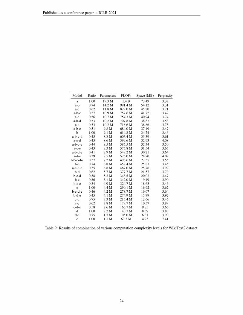
Table 9: Results of combination of various computation complexity levels for WikiText2 dataset.

24

h fl: computation and communication e f learning for

Documents