h : b based configuration eval uation for …

Published as a conference paper at ICLR 2017

HYPERBAND: BANDIT-BASED CONFIGURATION EVAL-UATION FOR HYPERPARAMETER OPTIMIZATION

Lisha Li∗, Kevin Jamieson∗∗, Giulia DeSalvo†, Afshin Rostamizadeh‡, and Ameet Talwalkar∗∗UCLA, ∗∗UC Berkeley, †NYU, and ‡Google{lishal,ameet}@cs.ucla.edu, [email protected]@cims.nyu.edu, [email protected]

ABSTRACT

Performance of machine learning algorithms depends critically on identifying agood set of hyperparameters. While recent approaches use Bayesian Optimiza-tion to adaptively select configurations, we focus on speeding up random searchthrough adaptive resource allocation. We present HYPERBAND, a novel algorithmfor hyperparameter optimization that is simple, flexible, and theoretically sound.HYPERBAND is a principled early-stoppping method that adaptively allocates a pre-defined resource, e.g., iterations, data samples or number of features, to randomlysampled configurations. We compare HYPERBAND with popular Bayesian Opti-mization methods on several hyperparameter optimization problems. We observethat HYPERBAND can provide more than an order of magnitude speedups overcompetitors on a variety of neural network and kernel-based learning problems.

1 INTRODUCTION

The task of hyperparameter optimization is becoming increasingly important as modern data analysispipelines grow in complexity. The quality of a predictive model critically depends on its hyperpa-rameter configuration, but it is poorly understood how these hyperparameters interact with eachother to affect the quality of the resulting model. Consequently, practitioners often default to eitherhand-tuning or automated brute-force methods like random search and grid search.

In an effort to develop more efficient search methods, the problem of hyperparameter optimization hasrecently been dominated by Bayesian optimization methods (Snoek et al., 2012; Hutter et al., 2011;Bergstra et al., 2011) that focus on optimizing hyperparameter configuration selection. These methodsaim to identify good configurations more quickly than standard baselines like random search byselecting configurations in an adaptive manner; see Figure 1(a). Existing empirical evidence suggeststhat these methods outperform random search (Thornton et al., 2013; Eggensperger et al., 2013; Snoeket al., 2015). However, these methods tackle a fundamentally challenging problem of simultaneouslyfitting and optimizing a high-dimensional, non-convex function with unknown smoothness, andpossibly noisy evaluations. To overcome these difficulties, some Bayesian optimization methodsresort to heuristics, at the expense of consistency guarantees, to model the objective function or speedup resource intensive subroutines.1 Moreover, these adaptive configuration selection methods areintrinsically sequential and thus difficult to parallelize.

An orthogonal approach to hyperparameter optimization focuses on speeding up configurationevaluation; see Figure 1(b). These methods are adaptive in computation, allocating more resourcesto promising hyperparameter configurations while quickly eliminating poor ones. Resources cantake various forms, including size of training set, number of features, or number of iterations foriterative algorithms. By adaptively allocating these resources, these methods aim to examine orders ofmagnitude more hyperparameter configurations than methods that uniformly train all configurations tocompletion, thereby quickly identifying good hyperparameters. While there are methods that combineBayesian optimization with adaptive resource allocation (Swersky et al., 2013; 2014; Domhan et al.,2015), we focus on speeding up random search as it offers a simple, parallelizable, and theoreticallyprincipled launching point and is shown to outperform grid search (Bergstra & Bengio, 2012).

1Consistency can be restored by allocating a fraction of resources to performing random search.

1


(a) Configuration Selection (b) Configuration Evaluation (c) Envelopes

Figure 1: (a) The heatmap shows the validation error over a two dimensional search space, withred corresponding to areas with lower validation error, and putative configurations selected in asequential manner as indicated by the numbers. (b) The plot shows the validation error as a functionof the resources allocated to each configuration (i.e., each line in the plot). Configuration evaluationmethods allocate more resources to promising configurations. (c) The validation loss as a function oftotal resources allocated for two configurations. The shaded areas bound the maximum distance fromthe terminal validation loss and monotonically decreases with the resource.

Our novel configuration evaluation method, HYPERBAND, relies on a principled early-stoppingstrategy to allocate resources, allowing it to evaluate orders of magnitude more configurations thanuniform allocation strategies. HYPERBAND is a general-purpose technique that makes minimalassumptions, unlike prior configuration evaluation approaches (Swersky et al., 2013; Domhan et al.,2015; Swersky et al., 2014; Gyorgy & Kocsis, 2011; Agarwal et al., 2011). In this work, we describeHYPERBAND, provide intuition for the algorithm through a detailed example, and present a widerange of empirical results comparing HYPERBAND with well established competitors. We also brieflydescribe the theoretical underpinnings of HYPERBAND, however a thorough theoretical treatment isbeyond the scope of this paper and is deferred to Li et al. (2016).

2 RELATED WORK

Bayesian optimization techniques model the conditional probability p(f |λ) of a configuration’sperformance on a metric f given a set of hyperparameters λ. For instance, SMAC uses random foreststo model p(f |λ) as a Gaussian distribution (Hutter et al., 2011). TPE is a non-standard Bayesianoptimization algorithm based on tree-structured Parzen density estimators (Bergstra et al., 2011). Athird popular method, Spearmint, uses Gaussian processes (GP) to model p(f |λ) and performs slicesampling over the GP’s hyperparameters (Snoek et al., 2012).

Adaptive configuration evaluation is not a new idea. Maron & Moore (1993) considered a settingwhere training time is negligible (e.g., k-nearest-neighbor classification) and evaluation on a largevalidation set is accelerated by evaluating on an increasing subset of the validation set, stoppingearly configurations that are performing poorly. Since subsets of the validation set provide unbiasedestimates of its expected performance, this is an instance of the stochastic best-arm identificationproblem for multi-armed bandits (see Jamieson & Nowak (2014) for a brief survey).

In contrast, this paper assumes that evaluation time is negligible and the goal is to early-stop long-running training procedures by evaluating partially trained models on the validation set. Previousapproaches either require strong assumptions or use heuristics to perform adaptive resource allocation.Several works propose methods that make strong assumptions on the convergence behavior of trainingalgorithms, providing theoretical performance guarantees under these assumptions (Gyorgy & Kocsis,2011; Agarwal et al., 2011; Swersky et al., 2013; 2014; Domhan et al., 2015; Sabharwal et al.,2016). Unfortunately, these assumptions are often hard to verify, and empirical performance candrastically suffer when they are violated. One recent work of particular interest proposes a heuristicbased on sequential analysis to determine stopping times for training configurations on increasingsubsets of the data (Krueger et al., 2015). However, it has a few shortcomings: (1) it is designedto speedup multi-fold cross-validation and is not significantly faster than standard holdout, (2) itis not an anytime algorithm and requires the set of configurations to be evaluated as an input, and(3) the theoretical correctness and empirical performance of this method are highly dependent on

2


a user-defined “safety-zone.”2 Lastly, in an effort avoid heuristics and strong assumptions, Sparkset al. (2015) proposed a halving style algorithm that did not require explicit convergence behavior,and Jamieson & Talwalkar (2015) analyzed a similar algorithm, providing theoretical guarantees andencouraging empirical results. Unfortunately, these halving style algorithms suffer from the n vsB/n issue which we will discuss in Section 3.

Finally, Klein et al. (2016) recently introduced Fabolas, a Bayesian optimization method that combinesadaptive selection and evaluation. Similar to Swersky et al. (2013; 2014), it models the conditionalvalidation error as a Gaussian process using a kernel that captures the covariance with downsamplingrate to allow for adaptive evaluation. While we intended to compare HYPERBAND with Fabolas, weencountered some technical difficulties when using the package3 and are working with the authors ofKlein et al. (2016) to resolve the issues.

3 HYPERBAND ALGORITHM

HYPERBAND extends the SUCCESSIVEHALVING algorithm proposed for hyperparameter optimiza-tion in Jamieson & Talwalkar (2015) and calls it as a subroutine. The idea behind SUCCESSIVE-HALVING follows directly from its name: uniformly allocate a budget to a set of hyperparameterconfigurations, evaluate the performance of all configurations, throw out the worst half, and repeatuntil one configurations remains. The algorithm allocates exponentially more resources to morepromising configurations. Unfortunately, SUCCESSIVEHALVING requires the number of configu-rations n as an input to the algorithm. Given some finite time budget B (e.g. an hour of trainingtime to choose a hyperparameter configuration), B/n resources are allocated on average acrossthe configurations. However, for a fixed B, it is not clear a priori whether we should (a) considermany configurations (large n) with a small average training time; or (b) consider a small number ofconfigurations (small n) with longer average training times.

We use a simple example to better understand this tradeoff. Figure 1(c) shows the validation loss as afunction of total resources allocated for two configurations with terminal validation losses ν1 and ν2.The shaded areas bound the maximum deviation from the terminal validation loss and will be referredto as “envelope” functions. It is possible to differentiate between the two configurations when theenvelopes diverge. Simple arithmetic shows that this happens when the width of the envelopes isless than ν2 − ν1, i.e. when the intermediate losses are guaranteed to be less than ν2−ν1

2 away fromthe terminal losses. There are two takeaways from this observation: more resources are needed todifferentiate between the two configurations when either (1) the envelope functions are wider or (2)the terminal losses are closer together.

However, in practice, the optimal allocation strategy is unknown because we do not have knowledgeof the envelope functions nor the distribution of terminal losses. Hence, if more resources arerequired before configurations can differentiate themselves in terms of quality (e.g., if an iterativetraining method converges very slowly for a given dataset or if randomly selected hyperparameterconfigurations perform similarly well) then it would be reasonable to work with a small numberof configurations. In contrast, if the quality of a configuration is typically revealed using minimalresources (e.g., if iterative training methods converge very quickly for a given dataset or if randomlyselected hyperparameter configurations are of low-quality with high probability) then n is thebottleneck and we should choose n to be large.

3.1 HYPERBAND

HYPERBAND, shown in Algorithm 1, addresses this “n versus B/n” problem by considering severalpossible values of n for a fixed B, in essence performing a grid search over feasible value of n.Associated with each value of n is a minimum resource r that is allocated to all configurations beforesome are discarded; a larger value of n corresponds to a smaller r and hence more aggressive earlystopping. There are two components to HYPERBAND; (1) the inner loop invokes SUCCESSIVEHALV-ING for fixed values of n and r (lines 3-9) and (2) the outer loop which iterates over different values

2The first two drawbacks prevent a full comparison to HYPERBAND on our selected empirical tasks, however,for completeness, we provide a comparison in Appendix A to Krueger et al. (2015) on some experimental tasksreplicated from their paper.

3The package provided by Klein et al. (2016) is available at https://github.com/automl/RoBO.

3

https://github.com/automl/RoBO


of n and r (lines 1-2). We will refer to each such run of SUCCESSIVEHALVING within HYPERBANDas a “bracket.” Each bracket is designed to use about B total resources and corresponds to a differenttradeoff between n and B/n. A single execution of HYPERBAND takes a finite number of iterations,and in practice can be repeated indefinitely.

HYPERBAND requires two inputs (1) R, the maximum amount of resource that can be allocated to asingle configuration, and (2) η, an input that controls the proportion of configurations discarded in eachround of SUCCESSIVEHALVING. The two inputs dictate how many different brackets are considered;specifically, smax + 1 different values for n are considered with smax = blogη(R)c. HYPERBANDbegins with the most aggressive bracket s = smax, which sets n to maximize exploration, subjectto the constraint that at least one configuration is allocated R resources. Each subsequent bracketreduces n by a factor of approximately η until the final bracket, s = 0, in which every configuration isallocated R resources (this bracket simply performs classical random search). Hence, HYPERBANDperforms a geometric search in the average budget per configuration to address the “n versus B/n”problem, at the cost of approximately smax+1 times more work than running SUCCESSIVEHALVINGfor a fixed n. By doing so, HYPERBAND is able to exploit situations in which adaptive allocationworks well, while protecting itself in situations where more conservative allocations are required.

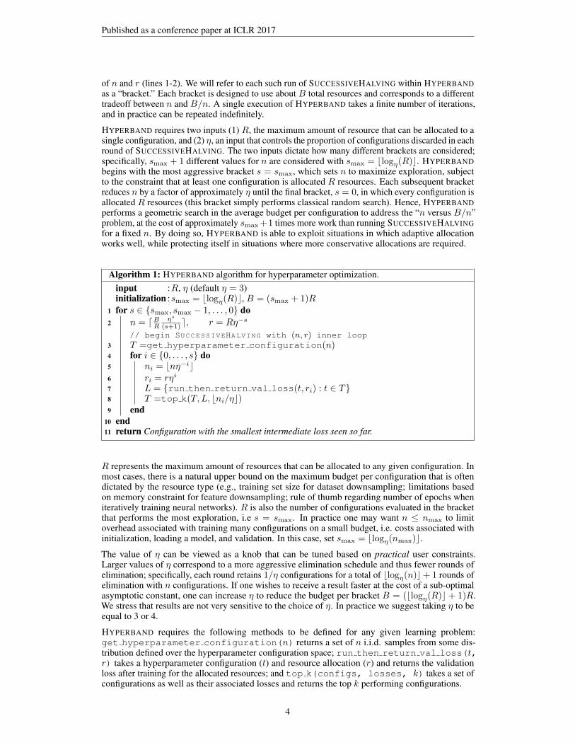
Algorithm 1: HYPERBAND algorithm for hyperparameter optimization.input :R, η (default η = 3)initialization :smax = blogη(R)c, B = (smax + 1)R

1 for s ∈ {smax, smax − 1, . . . , 0} do2 n = dBR

ηs

(s+1)e, r = Rη−s

// begin SUCCESSIVEHALVING with (n, r) inner loop3 T =get hyperparameter configuration(n)4 for i ∈ {0, . . . , s} do5 ni = bnη−ic6 ri = rηi

7 L = {run then return val loss(t, ri) : t ∈ T}8 T =top k(T, L, bni/ηc)9 end

10 end11 return Configuration with the smallest intermediate loss seen so far.

R represents the maximum amount of resources that can be allocated to any given configuration. Inmost cases, there is a natural upper bound on the maximum budget per configuration that is oftendictated by the resource type (e.g., training set size for dataset downsampling; limitations basedon memory constraint for feature downsampling; rule of thumb regarding number of epochs wheniteratively training neural networks). R is also the number of configurations evaluated in the bracketthat performs the most exploration, i.e s = smax. In practice one may want n ≤ nmax to limitoverhead associated with training many configurations on a small budget, i.e. costs associated withinitialization, loading a model, and validation. In this case, set smax = blogη(nmax)c.The value of η can be viewed as a knob that can be tuned based on practical user constraints.Larger values of η correspond to a more aggressive elimination schedule and thus fewer rounds ofelimination; specifically, each round retains 1/η configurations for a total of blogη(n)c+ 1 rounds ofelimination with n configurations. If one wishes to receive a result faster at the cost of a sub-optimalasymptotic constant, one can increase η to reduce the budget per bracket B = (blogη(R)c + 1)R.We stress that results are not very sensitive to the choice of η. In practice we suggest taking η to beequal to 3 or 4.

HYPERBAND requires the following methods to be defined for any given learning problem:get hyperparameter configuration(n) returns a set of n i.i.d. samples from some dis-tribution defined over the hyperparameter configuration space; run then return val loss(t,r) takes a hyperparameter configuration (t) and resource allocation (r) and returns the validationloss after training for the allocated resources; and top k(configs, losses, k) takes a set ofconfigurations as well as their associated losses and returns the top k performing configurations.

4


3.2 EXAMPLE APPLICATION WITH ITERATIONS AS A RESOURCE: LENET

We next present a simple example to provide intuition. We work with the MNIST dataset and optimizehyperparameters for the LeNet convolutional neural network trained using mini-batch SGD. Oursearch space includes learning rate, batch size, and number of kernels for the two layers of thenetwork as hyperparameters (details are shown in Table 3 in Appendix A).

We further define the number of iterations as the resource to allocate, with one unit of resourcecorresponding to one epoch or a full pass over the dataset. We set R to 81 and use the default value ofη = 3, resulting in smax = 4 and thus 5 brackets of SUCCESSIVEHALVING with different tradeoffsbetween n and B/n. The resources allocated within each bracket are displayed in Table 1.

s = 4 s = 3 s = 2 s = 1 s = 0i ni ri ni ri ni ri ni ri ni ri0 81 1 27 3 9 9 6 27 5 811 27 3 9 9 3 27 2 812 9 9 3 27 1 813 3 27 1 814 1 81

Table 1: Values of ni and ri for the brackets of HYPER-BAND when R = 81 and η = 3. Figure 2: Performance of individ-

ual brackets s and HYPERBAND.

Figure 2 compares the empirical performance of the different brackets of HYPERBAND if they wereused separately, as well as standard HYPERBAND (all results are averaged over 70 trials). In practicewe do not know a priori which bracket s ∈ {0, . . . , 4} will be most effective, and in this case neitherthe most (s = 4) nor least aggressive (s = 0) setting is optimal. However, note that HYPERBANDdoes nearly as well as the optimal bracket (s = 3) and vastly outperforms the baseline uniformallocation (i.e. random search), which is equivalent to bracket s = 0.

3.3 OVERVIEW OF THEORETICAL RESULTS

Although a detailed theoretical analysis is beyond the scope of this paper, we provide an intuitive,high-level description of theoretical properties of HYPERBAND. Suppose there are n configurations,each with a given terminal validation error νi for i = 1, . . . , n. Without loss of generality, index theconfigurations by performance so that ν1 corresponds to the best performing configuration, ν2 to thesecond best, and so on. Now consider the task of identifying the best configuration. The optimalstrategy would allocate to each configuration i the minimum resource required to distinguish it fromν1, i.e., enough so that the envelope functions depicted in Figure 1(c) bound the intermediate loss tobe less than νi−ν1

2 away from the terminal value. As shown in Jamieson & Talwalkar (2015) and Liet al. (2016), the budget required by SUCCESSIVEHALVING is in fact only a small factor away fromthis optimal approach because it capitalizes on configurations that are easy to distinguish from ν1.In contrast, the naive uniform allocation strategy, which allocates B/n to each configuration, has toallocate to every configuration the resource required to distinguish ν2 from ν1.

The relative size of the budget required for uniform allocation and SUCCESSIVEHALVING dependson the envelope functions bounding deviation from terminal losses as well as the distribution fromwhich νi’s are drawn. The budget required for SUCCESSIVEHALVING is smaller when the optimaln versus B/n tradeoff requires fewer resources per configuration. Hence, if the envelope functionstighten quickly as a function of resource allocated, or the average distances between terminal lossesis large, then SUCCESSIVEHALVING can be substantially faster than uniform allocation. Of coursewe do not have knowledge of either function in practice, so we will hedge our aggressivenesswith HYPERBAND. Remarkably, despite having no knowledge of the envelope functions or thedistribution of νi’s, HYPERBAND requires a budget that is only log factors larger than the optimal forSUCCESSIVEHALVING. See Li et al. (2016) for details.

5


0 10 20 30 40 50Multiple of R Used

0.18

0.20

0.22

0.24

0.26

0.28

0.30

0.32

Avera

ge T

est

Err

or

hyperband (finite)

SMAC

SMAC (Early Stop)

TPE

spearmint

random

random_2x

bracket s=4

(a) CIFAR-10


0.22

0.23

0.24

0.25

0.26

0.27

0.28

0.29

0.30

Avera

ge T

est

Err

or

(b) MRBI


0.03

0.04

0.05

0.06

0.07

0.08

0.09

0.10

Avera

ge T

est

Err

or

(c) SVHN

Figure 3: Average test error across 10 trials is shown in all plots. Label “SMAC early” corresponds toSMAC with the early stopping criterion proposed in Domhan et al. (2015) and label “bracket s = 4”corresponds to repeating the most exploratory bracket of HYPERBAND.

4 HYPERPARAMETER OPTIMIZATION EXPERIMENTS

In this section, we evaluate the empirical behavior of HYPERBAND with iterations, data subsamples,and features as resources. For all experiments, we compare HYPERBAND with three well knownBayesian optimization algorithms — SMAC, TPE, and Spearmint. Additionally, we show results forSUCCESSIVEHALVING corresponding to repeating the most exploration bracket of HYPERBAND.Finally for all experiments, we benchmark against standard random search and random 2×, which isa variant of random search with twice the budget of other methods.

4.1 EARLY STOPPING ITERATIVE ALGORITHMS FOR NEURAL NETWORKS

We study a convolutional neural network with the same architecture as that used in Snoek et al. (2012)and Domhan et al. (2015) from cuda-convnet. The search spaces used in the two previous worksdiffer, and we used a search space similar to that of Snoek et al. (2012) with 6 hyperparameters forstochastic gradient decent and 2 hyperparameters for the response normalization layers. In line withthe two previous works, we used a batch size of 100 for all experiments. For these experiments, wealso compare against a variant of SMAC named SMAC early that uses the early termination criterionproposed in Domhan et al. (2015) for neural networks. We view SMAC with early stopping to be acombination of adaptive configuration selection and configuration evaluation. See Appendix A formore details about the experimental setup.

Datasets: We considered three image classification datasets: CIFAR-10 (Krizhevsky, 2009), rotatedMNIST with background images (MRBI) (Larochelle et al., 2007), and Street View House Numbers(SVHN) (Netzer et al., 2011). CIFAR-10 and SVHN contain 32 × 32 RGB images while MRBIcontains 28× 28 grayscale images. The splits used for each dataset are as follows: (1) CIFAR-10 has40k, 10k, and 10k instances; (2) MRBI has 10k, 2k, and 50k instances; and (3) SVHN has close to600k, 6k, and 26k instances for training, validation, and test respectively. For all datasets, the onlypreprocessing performed on the raw images was demeaning.

HYPERBAND Configuration: For these experiments, one unit of resource corresponds to 100 mini-batch iterations. For CIFAR-10 and MRBI, R is set to 300 (or 30k total iterations). For SVHN, Ris set to 600 (or 60k total iterations) to accommodate the larger training set. η was set to 4 for allexperiments, resulting in 5 SUCCESSIVEHALVING brackets for HYPERBAND.

Results: Ten independent trials were performed for each searcher. For CIFAR-10, the results inFigure 3(a) show that HYPERBAND is more than an order of magnitude faster than its competitors.In Figure 6 of Appendix A, we extend the x-axis for CIFAR-10 out to 100R. The results showthat Bayesian optimization methods ultimately converge to similar errors as HYPERBAND. ForMRBI, HYPERBAND is more than an order of magnitude faster than standard configuration selectionapproaches and 5× faster than SMAC with early stopping. For SVHN, while HYPERBAND findsa good configuration faster, Bayesian optimization methods are competitive and SMAC with earlystopping outperforms HYPERBAND. This result demonstrates that there is merit to incorporatingearly stopping with configuration selection approaches.

6


Across the three datasets, HYPERBAND and SMAC early are the only two methods that consistentlyoutperform random 2×. On these datasets, HYPERBAND is over 20× faster than random searchwhile SMAC early is ≤ 7× faster than random search within the evaluation window. In fact, the firstresult returned by HYPERBAND after using a budget of 5R is often competitive with results returnedby other searchers after using 50R. Additionally, HYPERBAND is less variable than other searchersacross trials, which is highly desirable in practice (see Appendix A for plots with error bars).

For computationally expensive problems in high dimensional search spaces, it may make sense tojust repeat the most exploratory brackets. Similarly, if meta-data is available about a problem or itis known that the quality of a configuration is evident after allocating a small amount of resource,then one should just repeat the most exploration bracket. Indeed, for these experiments, repeatingthe most exploratory bracket of HYPERBAND outperforms cycling through all the brackets. In fact,bracket s = 4 vastly outperforms all other methods on CIFAR-10 and MRBI and is nearly tied withSMAC early for first on SVHN.

Finally, CIFAR-10 is a very popular dataset and state-of-the-art models achieve much better accuracythan what is shown in Figure 3. The difference in performance is mainly attributable to higher modelcomplexities and data manipulation (i.e. using reflection or random cropping to artificially increase thedataset size). If we limit the comparison to published results that use the same architecture and excludedata manipulation, the best human expert result for the dataset is 18% error and hyperparameteroptimized result is 15.0% for Snoek et al. (2012)4 and 17.2% for Domhan et al. (2015). These resultsare better than our results on CIFAR-10 because they use 25% more data by including the validationset and also train for more epochs. The best model found by HYPERBAND achieved a test error of17.0% when trained on the combined training and validation data for 300 epochs.

4.2 DATA DOWNSAMPLING KERNEL REGULARIZED LEAST SQUARES CLASSIFICATION

In this experiment, we use HYPERBAND with data samples as the resource to optimize the hyper-parameters of a kernel-based classification task on CIFAR-10. We use the multi-class regularizedleast squares classification model which is known to have comparable performance to SVMs (Rifkin& Klautau, 2004; Agarwal et al., 2014) but can be trained significantly faster. The hyperparametersconsidered in the search space include preprocessing method, regularization, kernel type, kernellength scale, and other kernel specific hyperparameters (see Appendix A for more details). HY-PERBAND is run with η = 4 and R = 400, with each unit of resource representing 100 datapoints.Similar to previous experiments, these inputs result in a total of 5 brackets. Each hyperparameteroptimization algorithm is run for ten trials on Amazon EC2 m4.2xlarge instances; for a giventrial, HYPERBAND is allowed to run for two outer loops, bracket s = 4 is repeated 10 times, and allother searchers are run for 12 hours.

Figure 4 shows that HYPERBAND returns a good configuration after just the first SUCCESSIVEHALV-ING bracket in approximately 20 minutes; other searchers fail to reach this error rate on averageeven after the entire 12 hours. Notably, HYPERBAND was able to evaluate over 250 configurationsin this first bracket of SUCCESSIVEHALVING, while competitors were able to evaluate only threeconfigurations in the same amount of time. Consequently, HYPERBAND is over 30× faster thanBayesian optimization methods and 70× faster than random search. Bracket s = 4 sightly outper-forms HYPERBAND but the terminal performance for the two algorithms are the same. Random 2×is competitive with SMAC and TPE.

4.3 FEATURE SUBSAMPLING TO SPEED UP APPROXIMATE KERNEL CLASSIFICATION

We next demonstrate the performance of HYPERBAND when using features as a resource, focusingon random feature approximations for kernel methods. Features are randomly generated using themethod described in Rahimi & Recht (2007) to approximate the RBF kernel, and these randomfeatures are then used as inputs to a ridge regression classifier. We consider hyperparameters ofa random feature kernel approximation classifier trained on CIFAR-10, including preprocessingmethod, kernel length scale, and l2 penalty. We impose an upper bound of 100k random featuresfor the kernel approximation so that the data will comfortably fit into a machine with 60GB of

4We were unable to reproduce this result even after receiving the optimal hyperparameters from the authorsthrough a personal communication.

7


0 100 200 300 400 500 600 700Minutes

0.40

0.45

0.50

0.55

0.60

0.65

Test

Err

or

hyperband

SMAC

TPE

random

random_2x

bracket s=4

Figure 4: Average test error of the best kernelregularized least square classification modelfound by each searcher on CIFAR-10. Thecolor coded dashed lines indicate when the lasttrial of a given searcher finished.

0 100 200 300 400 500 600 700Minutes

0.40

0.45

0.50

0.55

0.60

0.65

Test

Err

or

hyperband

SMAC

TPE

spearmint

random

random_2x

bracket s=4

Figure 5: Average test error of the best ran-dom features model found by each searcheron CIFAR-10. The test error for HYPERBANDand bracket s = 4 are calculated in every eval-uation instead of at the end of a bracket.

memory. Additionally, we set one unit of resource to be 100 features for an R = 1000, which gives5 different brackets with η = 4. Each searcher is run for 10 trials, with each trial lasting 12 hourson a n1-standard-16 machine from Google Cloud Compute. The results in Figure 5 show thatHYPERBAND is around 6x faster than Bayesian methods and random search. HYPERBAND performssimilarly to bracket s = 4. Random 2× outperforms Bayesian optimization algorithms.

4.4 EXPERIMENTAL DISCUSSION

For a given R, the most exploratory SUCCESSIVEHALVING round performed by HYPERBAND

evaluates ηblogη(R)c configurations using a budget of (blogη(R)c+1)R, which gives an upper boundon the potential speedup over random search. If training time scales linearly with the resource,the maximum speedup offered by HYPERBAND compared to random search is ηblogη(R)c

(blogη(R)c+1) . Forthe values of η and R used in our experiments, the maximum speedup over random search isapproximately 50× given linear training time. However, we observe a range of speedups from 6× to70× faster than random search. The differences in realized speedup can be explained by two factors:(1) the scaling properties of total evaluation time as a function of the allocated resource and (2) thedifficulty of finding a good configuration.

If training time is superlinear as a function of the resource, then HYPERBAND can offer higherspeedups. More generally, if training scales like a polynomial of degree p > 1, the maximum speedupof HYPERBAND over random search is approximately ηp−1−1

ηp−1 ηblogη(R)c. Hence, higher speedupswere observed for the the kernel least square classifier experiment discussed in Section 4.2 becausethe training time scaled quadratically as a function of the resource.

If 10 randomly sampled configurations is sufficient to find a good hyperparameter setting, then thebenefit of evaluating orders of magnitude more configurations is muted. Generally the difficulty of theproblem scales with the dimension of the search space since coverage diminishes with dimensionality.For low dimensional problems, the number of configurations evaluated by random search andBayesian methods is exponential in the number of dimensions so good coverage can be achieved; i.e.if d = 3 as in the features subsampling experiment, then n = O(2d = 8). Hence, HYPERBAND isonly 6× faster than random search on the feature subsampling experiment. For the neural networkexperiments however, we hypothesize that faster speedups are observed for HYPERBAND because thedimension of the search space is higher.

5 FUTURE WORK

We have introduced a novel bandit-based method for adaptive configuration evaluation with demon-strated competitive empirical performance. Future work involves exploring (i) embedding HYPER-BAND into parallel and distributed computing environments; (ii) adjusting for training methods withdifferent convergence rates; and (iii) combining HYPERBAND with non-random sampling methods.

8


REFERENCES

A. Agarwal, J. Duchi, P. L. Bartlett, and C. Levrard. Oracle inequalities for computationally budgetedmodel selection. In COLT, 2011.

A. Agarwal, S. Kakade, N. Karampatziakis, L. Song, and G. Valiant. Least squares revisited: Scalableapproaches for multi-class prediction. In ICML, 2014.

J. Bergstra and Y. Bengio. Random search for hyper-parameter optimization. In JMLR, 2012.

J. Bergstra et al. Algorithms for hyper-parameter optimization. In NIPS, 2011.

T. Domhan, J. T. Springenberg, and F. Hutter. Speeding up automatic hyperparameter optimization ofdeep neural networks by extrapolation of learning curves. In IJCAI, 2015.

K. Eggensperger et al. Towards an empirical foundation for assessing bayesian optimization ofhyperparameters. In NIPS Bayesian Optimization Workshop, 2013.

A. Gyorgy and L. Kocsis. Efficient multi-start strategies for local search algorithms. JAIR, 41, 2011.

F. Hutter, H. Hoos, and K. Leyton-Brown. Sequential model-based optimization for general algorithmconfiguration. In Proc. of LION-5, 2011.

K. Jamieson and R. Nowak. Best-arm identification algorithms for multi-armed bandits in the fixedconfidence setting. In Information Sciences and Systems (CISS), 2014 48th Annual Conference on,pp. 1–6. IEEE, 2014.

K. Jamieson and A. Talwalkar. Non-stochastic best arm identification and hyperparameter optimiza-tion. In AISTATS, 2015.

A. Klein, S. Falkner, S. Bartels, P. Hennig, and F. Hutter. Fast bayesian optimization of machinelearning hyperparameters on large datasets. arXiv preprint arXiv:1605.07079, 2016.

A. Krizhevsky. Learning multiple layers of features from tiny images. In Technical report, Departmentof Computer Science, Univsersity of Toronto, 2009.

T. Krueger, D. Panknin, and M. Braun. Fast cross-validation via sequential testing. Journal ofMachine Learning Research, 16:1103–1155, 2015.

H. Larochelle et al. An empirical evaluation of deep architectures on problems with many factors ofvariation. In ICML, 2007.

L. Li, K. Jamieson, G. DeSalvo, A. Rostamizadeh, and A. Talwalkar. Hyperband: A novel bandit-based approach to hyperparameter optimization. arXiv:1603.06560, 2016.

O. Maron and A. Moore. Hoeffding races: Accelerating model selection search for classification andfunction approximation. In NIPS, 1993.

Y. Netzer et al. Reading digits in natural images with unsupervised feature learning. In NIPSWorkshop on Deep Learning and Unsupervised Feature Learning, 2011.

A. Rahimi and B. Recht. Random features for large-scale kernel machines. In NIPS, 2007.

G. Ratsch, T. Onoda, and K.R. Muller. Soft margins for adaboost. Machine Learning, 42:287–320,2001.

R. Rifkin and A. Klautau. In defense of one-vs-all classification. JMLR, 2004.

A. Sabharwal, H. Samulowitz, and G. Tesauro. Selecting near-optimal learners via incremental dataallocation. In AAAI, 2016.

P. Sermanet, S. Chintala, and Y. LeCun. Convolutional neural networks applied to house numbersdigit classification. In ICPR, 2012.

J. Snoek, H. Larochelle, and R. Adams. Practical bayesian optimization of machine learningalgorithms. In NIPS, 2012.

9


J. Snoek et al. Bayesian optimization using deep neural networks. In ICML, 2015.

E. Sparks, A. Talwalkar, D. Haas, M. J. Franklin, M. I. Jordan, and T. Kraska. Automating modelsearch for large scale machine learning,. In Symposium on Cloud Computing, 2015.

K. Swersky, J. Snoek, and R. Adams. Multi-task bayesian optimization. In NIPS, 2013.

K. Swersky, J. Snoek, and R. P. Adams. Freeze-thaw bayesian optimization. arXiv:1406.3896, 2014.

C. Thornton et al. Auto-weka: Combined selection and hyperparameter optimization of classificationalgorithms. In KDD, 2013.

10


A ADDITIONAL EXPERIMENTAL RESULTS

In this section, we present a comparison of HYPERBAND with the CVST algorithm from Kruegeret al. (2015) and provide additional details for experiments presented in Section 3 and 4.

A.1 COMPARISON WITH CVST

The CVST algorithm from Krueger et al. (2015) focuses on speeding up standard k-fold cross-validation. We did not include it as one of the competitors in Section 4 because the experimentswe selected were too computational expensive for multi-fold cross-validation and CVST is not anany time algorithm. Nonetheless, the CVST algorithm is an interesting approach and was shown tohave promising empirical performance in Krueger et al. (2015). Hence, we performed a small scalecomparison modeled after their empirical studies between CVST and HYPERBAND.

We replicated the classification experiments in Krueger et al. (2015) that train a support vectormachine on the datasets from the IDA benchmark (Ratsch et al., 2001). All experiments wereperformed on Google Cloud Compute’s n1-standard-1 instances. Following Krueger et al.(2015), we evaluated HYPERBAND and CVST on the same 2d grid of 610 hyperparameters andrecorded the best test error and duration for 50 trials . The only modification we made to their originalexperimental setup was the data splits; instead of half for test and half for training, we used 1/11th fortest and 10/11th for training. HYPERBAND performed holdout evaluation using 1/10th of the trainingdata as the validation set. We set η = 3, and R was set for each dataset so that a minimum resourceof 50 datapoints is allocated to each configuration. Table 2 shows that CVST and HYPERBANDachieve comparable test errors (the differences are well within the error bars), while HYPERBAND issignificantly faster than CVST on all datasets. More granularly, while CVST on average has slightlylower mean error, HYPERBAND is within 0.2% of CVST on 5 of the 7 datasets. Additionally, foreach of the 7 datasets, HYPERBAND does as well as or better than CVST in over half of the trials.

CVST Hyperband RatioDataset Test Error Duration Test Error Duration Durationbanana 9.8%±1.6% 12.3±5.0 9.9%±1.5% 1.8±0.1 6.7±2.8german 26.0%±4.5% 2.7±1.1 27.6%±4.8% 0.7±0.0 4.1±1.7image 2.9%±1.1% 3.5±1.0 3.3%±1.4% 1.0±0.0 3.4±0.9splice 8.6%±1.8% 10.6±3.1 8.7%±1.8% 3.9±0.1 2.7±0.8

ringnorm 1.4%±0.4% 21.3±2.3 1.5%±0.4% 6.5±0.3 3.3±0.4twonorm 2.4%±0.5% 27.9±10.0 2.4%±0.5% 6.5±0.2 4.3±1.5waveform 9.3%±1.3% 13.7±2.7 9.5%±1.3% 2.9±0.2 4.8±1.0

Table 2: The test error and duration columns show the average value plus/minus the standard deviationacross 50 trials. Duration is measured in minutes and indicates how long it took each method toevaluate the grid of 610 hyperparameters used in Krueger et al. (2015). The ratio column shows theratio of the duration for HYPERBAND over that for CVST with associated standard deviation.

A.2 LENET EXPERIMENT

We trained the LeNet convolutional neural network on MNIST using mini-batch SGD. Code isavailable for the network at http://deeplearning.net/tutorial/lenet.html. Thesearch space for the LeNet example discussed in Section 3.2 is shown in Table 3.

Hyperparameter Scale Min MaxLearning Rate log 1e-3 1e-1Batch size log 1e1 1e3Layer-2 Num Kernels (k2) linear 10 60Layer-1 Num Kernels (k1) linear 5 k2

Table 3: Hyperparameter space for the LeNet application of Section 3.2. Note that the number ofkernels in Layer-1 is upper bounded by the number of kernels in Layer-2.

11

http://deeplearning.net/tutorial/lenet.html


A.3 EXPERIMENTS USING ALEX KRIZHEVSKY’S CNN ARCHITECTURE

For the experiments discussed in Section 4.1, the exact architecture used is the 18% model providedon cuda-convnet for CIFAR-10.5

Hyperparameter Scale Min MaxLearning Parameters

Initial Learning Rate log 5 ∗ 10−5 5Conv1 l2 Penalty log 5 ∗ 10−5 5Conv2 l2 Penalty log 5 ∗ 10−5 5Conv3 l2 Penalty log 5 ∗ 10−5 5FC4 l2 Penalty log 5 ∗ 10−3 500

Learning Rate Reductions integer 0 3Local Response Normalization

Scale log 5 ∗ 10−6 5Power linear 0.01 3

Table 4: Hyperparameters and associated ranges for the three-layer convolutional network.

Search Space: The search space used for the experiments is shown in Table 4. The learning ratereductions hyperparameter indicates how many times the learning rate was reduced by a factor of 10over the maximum iteration window. For example, on CIFAR-10, which has a maximum iteration of30,000, a learning rate reduction of 2 corresponds to reducing the learning every 10,000 iterations, fora total of 2 reductions over the 30,000 iteration window. All hyperparameters with the exception ofthe learning rate decay reduction overlap with those in Snoek et al. (2012). Two hyperparameters inSnoek et al. (2012) were excluded from our experiments: (1) the width of the response normalizationlayer was excluded due to limitations of the Caffe framework and (2) the number of epochs wasexcluded because it is incompatible with dynamic resource allocation.

Datasets: CIFAR-10 and SVHN contain 32×32 RGB images while MRBI contains 28×28 grayscaleimages. For all datasets, the only preprocessing performed on the raw images was demeaning. ForCIFAR-10, the training (40,000 instances) and validation (10,000 instances) sets were sampled fromdata batches 1-5 with balanced classes. The original test set (10,000 instances) is used for testing.For MRBI, the training (10,000 instances) and validation (2,000 instances) sets were sampled fromthe original training set with balanced classes. The original test set (50,000 instances) is used fortesting. Lastly, for SVHN, the train, validation, and test splits were created using the same procedureas that in Sermanet et al. (2012).

Computational Considerations: The experiments took the equivalent of over 1 year of GPU hourson NVIDIA GRID K520 cards available on Amazon EC2 g2.8xlarge instances. We set a totalbudget constraint in terms of iterations instead of compute time to make comparisons hardwareindependent.6 Comparing progress by iterations instead of time ignores overhead costs not associatedwith training like cost of configuration selection for Bayesian methods and model initializationand validation costs for HYPERBAND. While overhead is hardware dependent, the overhead forHYPERBAND is below 5% on EC2 g2.8xlarge machines, so comparing progress by time passedwould not impact results significantly.

Due to the high computational cost of these experiments, we were not able to run all searchersout to convergence. However, we did double the budget for each trial of CIFAR-10 to allow for acomparison of the searchers as they near convergence. Figure 6 shows while Bayesian optimizationmethods achieve similar performance as HYPERBAND and SUCCESSIVEHALVING, it takes themmuch longer to achieve a comparable error rate.

Comparison with Early Stopping: Adaptive allocation for hyperparameter optimization can bethought of as a form of early stopping where less promising configurations are halted before comple-tion. Domhan et al. (2015) propose an early stopping method for neural networks and combine it

5The model specification is available at http://code.google.com/p/cuda-convnet/.6Most trials were run on Amazon EC2 g2.8xlarge instances but a few trials were run on different machines

due to the large computational demand of these experiments.

12

http://code.google.com/p/cuda-convnet/



0.18

0.20

0.22

0.24

0.26

0.28

0.30

0.32

Avera

ge T

est

Err

or

hyperband (finite)

SMAC

SMAC (Early Stop)

TPE

spearmint

random

random_2x

bracket s=4

(a) CIFAR-10


0.22

0.23

0.24

0.25

0.26

0.27

0.28

0.29

0.30

Avera

ge T

est

Err

or

(b) MRBI


0.03

0.04

0.05

0.06

0.07

0.08

0.09

0.10

Avera

ge T

est

Err

or

(c) SVHN

Figure 6: Average test error across 10 trials is shown in all plots. Error bars indicate the maximumand minimum ranges of the test error corresponding to the model with the best validation error

with SMAC to speed up hyperparameter optimization. Their method stops training a configurationif the probability of the configuration beating the current best is below a specified threshold. Thisprobability is estimated by extrapolating learning curves fit to the intermediate validation error lossesof a configuration. If a configuration is terminated early, the predicted terminal value from theestimated learning curves is used as the validation error passed to the hyperparameter optimizationalgorithm. Hence, if the learning curve fit is poor, it could impact the performance of the configura-tion selection algorithm. While this approach is heuristic in nature, it does demonstrate promisingempirical performance so we included SMAC with early termination as a competitor. We used theconservative termination criterion with default parameters and recorded the validation loss every400 iterations and evaluated the termination criterion 3 times within the training period (every 8kiterations for CIFAR-10 and MRBI and every 16k iterations for SVHN).7 Comparing performance bythe total multiple of R used is conservative because it does not account for the time spent fitting thelearning curve in order to check the termination criterion.

A.4 KERNEL CLASSIFICATION EXPERIMENTS

We trained the regularized least-squares classification model using a block coordinate descent solver.Our models take less than 10 minutes to train on CIFAR-10 using an 8 core machine, while the defaultSVM method in Scikit-learn is single core and takes hours. Table 5 shows the hyperparametersand associated ranges considered in the kernel least squares classification experiment discussed in

7We used the code provided at https://github.com/automl/pylearningcurvepredictor.

13


Hyperparameter Type Valuespreprocessor Categorical min/max, standardize, normalizekernel Categorical rbf, polynomial, sigmoidC Continuous log [10−3, 105]gamma Continuous log [10−5, 10]degree if kernel=poly integer [2,5]coef0 if kernel=poly,sigmoid uniform [-1.0, 1.0]

Table 5: Hyperparameter space for kernel regularized least squares classification problem discussedin Section 4.2.

Section 4.2. The cost term C is divided by the number of samples so that the tradeoff between thesquared error and the l2 penalty would remain constant as the resource increased (squared error issummed across observations and not averaged). The regularization term λ is equal to the inverse ofthe scaled cost term C. Additionally, the average test error with associated minimum and maximumranges across 10 trials are show in Figure 7.

0 100 200 300 400 500 600 700Minutes

0.40

0.45

0.50

0.55

0.60

0.65

Test

Err

or

hyperband

SMAC

TPE

random

random_2x

bracket s=4

Figure 7: Average test error of the best kernel regularized least square classification model foundby each searcher on CIFAR-10. The color coded dashed lines indicate when the last trial of a givensearcher finished. Error bars correspond to observed minimum and maximum test error across 10trials.

Hyperparameter Type Valuespreprocessor Categorical none, min/max, standardize, normalizeλ Continuous log [10−3, 105]gamma Continuous log [10−5, 10]

Table 6: Hyperparameter space for random feature kernel approximation classification problemdiscussed in Section 4.3.

Table 6 shows the hyperparameters and associated ranges considered in the random features kernelapproximation classification experiment discussed in Section 4.3. The regularization term λ isdivided by the number of features so that the tradeoff between the squared error and the l2 penaltywould remain constant as the resource increased. Additionally, the average test error with associatedminimum and maximum ranges across 10 trials are show in Figure 8.

14


0 100 200 300 400 500 600 700Minutes

0.40

0.45

0.50

0.55

0.60

0.65

Test

Err

or

hyperband

SMAC

TPE

spearmint

random

random_2x

bracket s=4

Figure 8: Average test error of the best random features model found by each searcher on CIFAR-10.The test error for HYPERBAND and bracket s = 4 are calculated in every evaluation instead of atthe end of a bracket. Error bars correspond to observed minimum and maximum test error across 10trials.

15

h : b based configuration eval uation for …

Documents