Gyro-Based Multi-Image Deconvolution for Removing Handshake Blur

Sung Hee Park Marc LevoyStanford University

shpark7@stanford.edu levoy@cs.stanford.edu

Abstract

Image deblurring to remove blur caused by camerashake has been intensively studied. Nevertheless, mostmethods are brittle and computationally expensive. In thispaper we analyze multi-image approaches, which captureand combine multiple frames in order to make deblur-ring more robust and tractable. In particular, we comparethe performance of two approaches: align-and-averageand multi-image deconvolution. Our deconvolution is non-blind, using a blur model obtained from real camera motionas measured by a gyroscope. We show that in most situ-ations such deconvolution outperforms align-and-average.We also show, perhaps surprisingly, that deconvolution doesnot benefit from increasing exposure time beyond a certainthreshold. To demonstrate the effectiveness and efficiency ofour method, we apply it to still-resolution imagery of nat-ural scenes captured using a mobile camera with flexiblecamera control and an attached gyroscope.

1. IntroductionImage blur due to camera shake is one of the main rea-

sons people discard their photos. Camera shake becomescritical in low-light situations, where long exposure timesare required, or when the camera motion is amplified bytelephoto optics. To reduce the amount of blur caused bycamera shake, two approaches are commonly used: align-and-average and image deblurring. Although they aim tosolve the same problem, they are built on different capturestrategies. Align-and-average captures multiple blur-freebut noisy images using a short exposure time, and mergesthem after alignment. On the other hand, image deblurringuses a long exposure time to capture a clean but blurry im-age and recovers the sharp image using deblurring. How-ever, there exists a middle ground between two extremeends of capture strategy. A set of images can be capturedwith intermediate exposure time, hence some small amountof blur, and jointly deconvolved to recover the latent image.

In this paper, we propose a multi-image deblurring sys-tem that combines two existing techniques: gyroscope-

based camera motion estimation and non-blind multi-imagedeconvolution. A burst of images is captured while the gy-roscope data is recorded simultaneously. We use a drift cor-rection method to remove bias from our gyroscope data. Bymeasuring camera motion and the scene as accurately as wecan, we improve the robustness of deconvolution.

A key question about any multi-image deblurringmethod is: for a given total capture time, how many im-ages should be captured, and what should their exposuretimes be? Shorter exposures suffer from worse read noiseand photon shot noise, while longer exposures suffer fromincreased handshake blur. To model this tradeoff, we definea noise amplification factor γ, which quantifies the increasein noise after multi-image deconvolution is performed. Weshow that for long exposures, γ grows linearly with expo-sure time. As a result, increasing exposure time does nothelp because additional blur cancels the increased signal tonoise ratio (SNR) due to less photon shot noise in the longerexposure.

Based on this observation, we compare the performanceof align-and-average and multi-image deblurring to findthe best capture strategy in various photographic situations.With the help of simulation, we show how performance isaffected by factors such as scene brightness, focal lengthof optics (hence field of view), sensor read noise, exposuretime, analog gain, number of shots, and so on. We thenformulate guidelines to help users to determine how to cap-ture and process images to get the best output in real-worldsituations.

2. Related WorkBlind image deblurring methods suffer from lack of in-

formation to recover the latent image. Even with the help ofmultiple images or image priors, blind methods are consid-ered brittle. Joshi et al. [3] proposed an effective solutionby using an inertial measurement unit to directly measurecamera motion. We adopt their method for motion estima-tion, but with two modifications. First, we only use gyro-scope data, not accelerometer data, because rotation is thedominant factor that causes blur [7]. Second, our methodperforms the drift correction on gyroscope data; otherwise,

accumulated bias causes non-negligible drift when long ex-posure times are used.

Comparing the capture strategies for camera motion de-blurring has been studied by Zhang et al. [9]. Their analysisconcludes that align-and-average works better than single-image deconvolution. Boracchi and Foi [1] made the similarobservation that restoration error of single-image deconvo-lution stabilizes after reaching a minimum. However, theseresults are limited to the single-image approach, while wefocus on the case when multiple images are used.

3. Image Formation with Camera MotionThe principal drawback of using a short exposure time

in low light is image noise. Lengthening the exposure de-creases noise, but increases handshake blur. It is thereforeimportant that we define a noise model that allows us tohandle handshake blur. We begin by describing an imagenoise model for when the camera is stable, then we extendit to include the effect of camera motion.

3.1. Image Noise Model

Given analog gain g and exposure time t, with scenebrightness Φ, we use a linear imaging model to describeraw pixel values of image Y as the sum of noise-free imageX and the Gaussian noise N with standard deviation σN .Specifically, the SNR of a captured image Y is written as

SNR(Y ) =X

σN=

c1gtΦ√c2g2tΦ + g2σ2

r0 + σ2r1

. (1)

where c1 and c2 are conversion factors, with σ2r0 and σ2

r1representing the variance of readout noise applied beforeand after analog amplification, respectively [2].

3.2. From Camera Motion to Image Blur

Let’s extend this image noise model to incorporate cam-era motion while assuming no motion of objects in thescene. With camera motion, a point in the scene contributesto multiple pixels along the motion path. We assume alsothat camera motion is dominated by rotation − a commonassumption in image stabilization systems, and valid forsufficiently distant scenes. This allows us to represent theoff-axis angular rotation at point r as

R∆θo {r} = R∆θ(r − o) + o (2)

where R∆θ is a 3-axis rotation matrix for angular rotation∆θ, and o = (ox, oy, oz)

T is the rotation center. If a rota-tion ∆θ(ts, tt) is applied during time window [ts, tt], thenjth pixel pj = (xj , yj)T in the image plane is shifted to(xj ′, yj ′)T by the following relation:

α(xj ′, yj ′, 1)T = MfR∆θ(ts,tt)o {M−1

f (xj , yj , 1)T } (3)

where α is an unknown scaling factor andMf is the cameraintrinsic matrix, which depends mainly on focal length f .

Given this model for rotation, the rotation-blurred image Ycan be formulated as the sum of the time integration of allgeometrically transformed latent images during the expo-sure window [ts, tt] plus noise. We assume a local windowof blurry image Yi around pj contains uniform blur, whichis represented as

Yi = Kji ⊗X +Ni (4)

where Kji is the 2-D blur kernel, ⊗ is the 2-D convolution

operator and i denotes the input image index when multi-ple images are available. The kernel Kj

i is specified by theexposure window [tis, t

it], which can be expressed in terms

of capture parameters. The two ends of the window are de-fined as tis = t1s+(i−1)tft and tit = tis+texp, where texp isthe exposure time of a single shot and the frame time tft isthe gap between frames. Note that all entries in Kj

i sum toone. Also, t1s, the time when the first exposure starts, is setas the reference time so that relative rotation between inputimages are preserved in the kernel.

4. Modeling the Performance of Non-BlindMulti-Image Deconvolution

When the blur kernel is available, the latent image can berecovered via non-blind multi-image deconvolution. Mod-eling the performance of this deconvolution is not trivialbecause two factors are mixed together: camera shake blurand the scene. Although it is hard to estimate the influenceof the scene on deconvolution, modeling the effect of bluris tractable in the non-blind case.

In this section, we derive a noise amplification factor thatquantifies the performance of deconvolution based on thecharacteristics of this blur. Wiener deconvolution [8] is astandard frequency domain method for estimating a latentimageX from a blurry image Yi where the image formationmodel is given as Equation 4. By minimizing the expecta-tion of squared estimation error E

∣∣X̄ − X ∣∣2, we get

X̄ =

∑ni=1

1σ2Ni

K∗iYi∑nk=1

1σ2Nk

|Kk|2 + 1/ |X |2(5)

where X̄ is the optimum estimate of X , Ki is the knownblur kernel, n is the number of images, X , X̄ , Ki, andYi denote the Fourier transforms of X , X̄ , Ki, and Yi,respectively, |X |2 is the power spectrum of X , Ni is thewhite Gaussian noise in the frequency domain with vari-ance σ2

Ni= nunvσ

2Ni

, where nu and nv are the numberof pixels in each dimension in the frequency domain. ByParseval’s theorem, we can calculate total mean square er-ror (MSE) between X and X̄ over the whole image in the

frequency domain as

MSE(X̄) =1

n2un

2v

∑u,v

1∑nk=1

1σ2Nk

|Kk|2 + 1/ |X |2. (6)

To get some insight into this deconvolution procedure,let’s consider the case when all input images are capturedwith the same exposure time t and analog gain g. In thiscase, assume that the noise statistics for all images are iden-tical, σ2

Ni= σ2

N . If we assume no prior on the image statis-tics, as is the case for an unbiased optimal estimator, thenEquation 6 reduces to

MSE(X̄) = γσ2N

n(7)

where γ is the noise amplification factor defined as

γ =1

nunv

∑u,v

11n

∑ni=1 |Ki(u, v)|2

(8)

and corresponding SNR is given by

SNR(X̄) =

√n√γ

c1gtΦ√c2g2tΦ + g2σ2

r0 + σ2r1

. (9)

Note that γ quantifies the increase in high frequency noisewhen average power spectrum of the blur kernels is invertedin the deconvolution, and this factor is only dependent onthe characteristics of the blur applied to the system.

When image priors are used in deconvolution, therestoration error depends on the statistics of the scene, and afrequency domain analysis is not possible. When such pri-ors are used, we instead empirically measure performanceby estimating MSE in the spatial domain, assuming theground truth scene is available.

5. Characterization of Real Blur Caused byCamera Motion

In this section we focus on understanding handshake blurin real-world situations. Our main tool for this analysis willbe the noise amplification factor defined in Section 4. Themain challenge is that the blur is affected by various factors:exposure settings (exposure time, frame-to-frame time, andnumber of shots), user, type of camera (weight, grip type,optics, and pixel size), and so on. To explore this high-dimensional parameter space, we use simulation to buildan empirical model based on real measurements of camerashake.

As a start, we built a database of camera shake by col-lecting 100 sequences of real camera motion. Each userwas asked to hold a tablet steady for a 20-second exposure,while we recorded images and gyroscope streams. Thisdatabase allows us to create independent samples of cam-era motion by randomly selecting a small slice from a gyro-scope stream. Then, we can simulate various image capture

1 4 16 63 250 10000

5

10

15

20

25

30

texp (ms)

γ̄(dB)

n=1n=2n=4n=8n=16

(a) Number of shots n

1 4 16 63 250 1000

−35

−30

−25

−20

texp (ms)

t exp/γ̄(dB)

n=1n=2n=4n=8n=16

(b) Number of shots n

1 4 16 63 250 1000

−30

−25

−20

texp (ms)

t exp

/γ̄(dB)

User 1User 2User 3User 4User 5

n=2

n=8

(c) User

1 4 16 63 250 1000

−30

−25

−20

texp (ms)

t exp

/γ̄(dB)

no frame gaplong frame gap

n=2

n=8

(d) Frame time tft

1 4 16 63 250 1000

−35

−30

−25

−20

texp (ms)

t exp

/γ̄(dB)

32mm64mm128mm

(e) Focal length f

1 4 16 63 250 1000

−35

−30

−25

−20

texp (ms)

t exp

/γ̄(dB)

uncorrelated blurreal blur

(f) Demonstration of uncorrelated blur

Figure 1: Average noise amplification factor γ̄ measuredfrom simulation based on real camera motion. Each plotshows how γ̄ varies when a different parameter is changedas denoted by the plot captions. (a) shows γ̄ while (b)-(f)plot the ratio between γ̄ and per-image exposure time texp.Note that the ratio becomes constant for long exposures inall cases, which means that γ̄ increases linearly with texp.The relation comes from the fact that the blurs become un-correlated. (f) shows that consecutive blur kernels are un-correlated when texp is longer than ∼50ms.

scenarios, and evaluate γ̄, the noise amplification factor av-eraged over different camera shakes.

Figure 1 shows how average noise amplification factor γ̄is related to exposure time under various combination ofparameter settings. When texp is very small, γ̄ is closeto 1 because no blur exists as shown in Figure 1a. Notethat γ̄ increases with exposure time as image becomes moreblurry. However, more images reduces γ̄ because miss-ing frequency components in an image can be preserved inother images, which is visualized in Figure 2. The impor-tant observation is that γ̄ grows linearly with texp as shownin Figure 1b: the ratio between γ̄ and texp remains constantif the exposure time per shot is long enough. This relationis more obvious when n is large, and was consistently ob-served among different users and independent of the cam-

Image 1 2 3 4 5 6 7 8

(a) Blur kernels and their power spectran=1 n=2 n=3 n=4 n=5 n=6 n=7 n=8

(b) Average power spectrum of n imagesn=1 n=2 n=4 n=8

(c) Multi-image deconvolution applied to n images

Figure 2: An example of n-image deconvolution. (a) Thetop row shows a set of eight consecutive blur kernels from asingle instrumented handheld capture, and the bottom rowvisualizes their power spectrum. Note that different shapesof blur capture different frequency information. (b) Multi-image deconvolution is applied using n images without anypriors, to show the improvement when more images areused. As these power spectra show, adding more imagesfill in missing frequency components. Although no prior isused, the output images in (c) are not severely degraded bynoise when at least two images are used.

era’s focal length.We can explain this trend mathematically for large n and

t as follows. Let’s define the average power spectrum ofblur kernel as

P̄t =1

ni

∑i

|Ki,t|2 (10)

where Ki,t denotes ith sample of blur kernel for exposuretime t, Ki,t is the Fourier transform of Ki,t, ni is the num-ber of samples, and assume P̄t converges for large ni. Let’sthink of an image as the sum of first and second-half imageswith the same exposure time of 1

2 t. Then, we can split theblur kernel Ki,t into two as

Ki,t =1

2

(Ki1,

t2

+Ki2,t2

)(11)

where i1 and i2 denotes the index corresponds to first andsecond-half of i, respectively. Then, the power spectrum ofKi,t can be approximated as

|Ki,t|2 ≈1

4

(∣∣∣Ki1, t2 ∣∣∣2 +∣∣∣Ki2, t2 ∣∣∣2

)(12)

if we assume the crosscorrelation term is negligible because

no blur (γ̄ = 1) large blur (γ̄ ∝ t)read noisedominant SNR ∝

√ngt SNR ∝

√ng√t

photon noisedominant SNR ∝

√nt SNR ∝

√n

Table 1: Summary of the performance of multi-image de-convolution in various capture situations.

consecutive blur kernels become uncorrelated for relativelylong t. Then, we get the recursive relation for average powerspectrum P̄t = 1

2 P̄ t2

, which leads to γ̄n,t = 2γ̄n, t2 for largen. This shows the linear relation for large n and t:

γ̄n,t ∝ t. (13)

To verify the assumption that blurs are uncorrelated forlarge t, we evaluate γ̄ by using the approximation in Equa-tion 12, and compare it with the curve shown in Figure 1bfor n = 16. Figure 1f shows that they agree well when ex-posure time is longer than ∼50ms, and proves the assump-tion. Figure 1d shows another effect that uncorrelated blurshave on γ̄: uncorrelated blurs reduce γ̄ compared to cor-related ones because they preserve frequency componentsthat are complementary to each other. Longer frame-to-frame time makes the blurs less correlated, which results insmaller γ̄ shown in Figure 1d. Note that we can generallyassume blurs are uncorrelated after a certain time for anycamera or any user. Thus, the linear relation in Equation 13holds for any camera shake for large n and t.

6. Analysis of Capture Strategies6.1. Performance of Capture Strategies

With the blur model obtained in Section 5, we evalu-ate the image quality after multi-image deconvolution is ap-plied. To begin, let’s consider the case in which the perfor-mance is modeled by the blur applied to system, without as-suming any image priors. The relationships between outputSNR and various capture parameters can be obtained fromEquation 9 and Equation 13, and are summarized in Table 1.The first row in Table 1 assumes that read noise after ampli-fication is dominant. Note that if no blur exists (first columnof Table 1), then the analysis reduces to the case of align-and-average. When photon noise is dominant and large bluris involved (lower right cell of Table 1), then the SNR doesnot improve with exposure time, because additional blur in-troduced during the exposure cancels the improvement inSNR due to reduced shot noise in input images. In otherwords, longer exposures are preferable, at least to the pointwhere handshake blur becomes intolerable, and if read noiseis dominant, then this switchover point happens at a longerexposure time.

Let us now consider what effect image priors might have

in the analysis. We compare two approaches in removingcamera shake: align-and-average (AA) and multi-image de-convolution (MD). We test both cases with and without as-suming image priors. To make a fair comparison betweenAA and MD when image priors are used, we apply an ad-ditional denoising step on the output of AA by applyingEquation 5 with Ki = 1 and the Gaussian prior to sup-press the same amount of noise as in MD. The simulationis done on various scenes, and the performance is evalu-ated by the peak signal-to-noise ratio (PSNR) which is av-eraged over many trials with varying camera motions. Twoexamples are shown in Figure 3, in which we assume eightimages are captured with a unity analog gain. We observethat when the same parameters and image prior are used,then MD performs better than AA as shown in Figure 3dand 3f for the Gaussian prior. The improvement in PSNRof MD approaches a horizontal asymptote as exposure timebecomes sufficiently long, as discussed in Section 5. In-troducing a prior improves the PSNR but it does not sig-nificantly change the relation to exposure time as shown inTable 1. As a result, an analysis based on the noise amplifi-cation factor can still help estimate the performance of MDeven when image priors are used.

6.2. Choosing Capture Strategies

Based on our analysis, a list of guidelines can be ob-tained, which helps determine the best capture strategy andreconstruction method for various environments. We as-sume the user has control of n, g, and texp, and faces vari-ability in scene statistics and dynamic range, and cameranoise model, optics, and so on. To understand the effectof each factor, we performed simulation on the Cafe scene,changing one axis of the parameter space at a time. Figure4a shows that focal length strongly affects the range of ex-posure times in which AA is effective because handshakeblur, which remains after AA, is worse for longer focallengths. This observation gives an upper bound on exposuretimes appropriate for AA. On the other hand, a lower boundon exposure exists because accurate alignment is predicatedon having low noise. AA is expected to work only whenthese two conditions are satisfied. On the other hand, MDprefers longer exposures to the point at which read noiseis negligible and handshake blur is intolerable. This pointcomes at shorter exposure times if scenes are brighter ormore images are captured, as shown in Figure 4c and 4b.In addition, when long exposures are used, texp should becontrolled to avoid over-exposing bright regions.

In many situations, AA is preferred to MD because theformer has lower computational cost. A good strategy is tofind a parameter set that gives desired image quality withAA, although it may not be possible for certain scenes. Us-ing higher analog gain or capturing more images helps im-prove the performance of AA, but the choice of g and n is

(a) Cafe (b) Office

1 4 16 63 250 1000

30

40

50

texp (ms)

PSNR

(dB)

MDAA

(c) Cafe, no prior

1 4 16 63 250 1000

30

40

50

texp (ms)

PSNR

(dB)

MD+SMD+GAA+G

(d) Cafe, using priors

1 4 16 63 250 1000

30

40

50

texp (ms)

PSNR

(dB)

MDAA

(e) Office, no prior

1 4 16 63 250 1000

30

40

50

texp (ms)

PSNR

(dB)

MD+SMD+GAA+G

(f) Office, using priors

Figure 3: The performance of align-and-average (AA) andmulti-image deconvolution (MD) with image priors. Twoexample scenes are shown in (a)(b). The curves in (c)-(f) aresimilar to Figure 1, but this time with priors. (c)(e) are ob-tained with no prior applied, while (d)(f) show the improve-ment when image priors are employed. The sparse prior(S) shown with the blue curve gives slightly more improve-ment than the Gaussian prior (G) in green. A small regionof output images for different exposure times is shown. Theinsets in red boxes correspond to the output of AA whilegreen boxes correspond to the output from MD. The per-formance follows the analysis in Table 1 even when imagepriors are used.

also bounded by various factors. For example, the effectiverange of analog gain is restricted by the presence of readnoise added before analog amplification. Also, the memorybuffer in the camera system, which is used to store capturedimages before they are merged, has a limited size, restrict-ing n from above. Finally, n is bounded by the total capturetime during which the photographer can expect the scene to

1 4 16 63 250 1000

30

40

50

texp (ms)

PSNR

(dB)

32 mm64 mm128 mm

(a) Focal length f

1 4 16 63 250 1000

30

40

50

texp (ms)

PSNR

(dB)

n=4n=8n=16

(b) Number of shot n

1 4 16 63 250 1000

30

40

50

texp (ms)

PSNR

(dB)

0.5x1x2x

(c) Scene brightness

1 4 16 63 250 1000

30

40

50

texp (ms)

PSNR

(dB)

1x gain2x gain4x gain

(d) Analog gain g

Figure 4: The effect of changing each parameter on the per-formance of align-and-average (red) and multi-image de-convolution (green). Results are from simulation, and allcases assume a Gaussian prior. Focal length strongly affectsthe range where align-and-average is effective as shown in(a). Other parameters shown in (b)-(d) change the ratio be-tween read noise and photon noise.

hold still. These various limitations restrict the use of AAin some environments, where MD can provide an alternativewith better performance.

7. Image Deblurring SystemIn addition to the foregoing analysis, which was based

largely on simulations, we have built a system for capturingimage and gyroscope data at high speed and applying ourdeblurring methods. Our system supports a flexible cap-ture configuration and records images and gyroscope datasimultaneously, and our software pipeline performs cameramotion estimation, drift correction, image deblurring, andimage post-processing.

7.1. Hardware Platform

We implemented our capture application on an NVIDIATegra 3 Android developer tablet. We modified the tablet torigidly attach an Atmel UC3-A3 Xplained and InvensenseMPU-6050 sensor board to obtain unfiltered raw sensordata. The sensor data is sent to the tablet through a USBconnection at a maximum rate of 750 Hz. The tablet cap-tures 5M-pixel raw data at a maximum rate of 4 fps. We em-ploy standard photometric and geometric calibration proce-dures to find the parameters of the image formation model.

(a) Blur kernels (b) Without correction (c) With correction

Figure 5: The effect of applying gyroscope drift correctionon image deblurring. (a) First four blur kernels of eightblurry images are shown. The gap between the red and yel-low kernels is due to drift. (b)(c) The output of image de-blurring significantly improves when drift is corrected.

7.2. Camera Motion Estimation using Gyroscope

The sensor data from our gyroscope requires addi-tional processing to estimate correct rotational motion de-scribed in Section 3.2. In particular, the gyroscope suf-fers from unstable bias, which appears as drift in therotational data. Moreover, this drift accumulates withlonger exposures. The standard deviation of the samples is(0.21, 0.12, 0.17)◦/s, which produces more than a pixel ofdeviation if the total capture time is longer than 1

6s for oursystem. Also, there exists an unknown time delay betweenimage and gyroscope data.

We model the angular rotation by accumulating the in-cremental changes given as

∆θ(t, t+ ∆t) = (ω(t+ td) + ωd)∆t (14)

where ω(t) is the rate of rotation measured with gyroscope,td is the time delay, ωd is the bias which causes drift, and∆t denotes the time interval between gyroscope samples.Based on the model, we propose a drift correction algorithmthat is applied whenever capture takes place. The algorithmestimates the time delay td, the bias ωd and the rotationcenter o by comparing measured camera motion with im-age data, where o is assumed to be constant during captureand oz is zero. To begin, we find the input image Yiref thatis observed to be sharpest. This is done by estimating theblur kernel of ith image at the image center and by pickingthe one that has maximum spatial variance. Then, we findnc image blocks that contain the region with strong cor-ner response in Yiref and denote the center of the blocks ascj . We formulate the kernel estimation as the minimizationproblem in which the objective function is defined as

argminωd,ox,oy,td

∑i6=iref

∑j

‖W ji (Kj

iref⊗Yi−Kj

i ⊗Yiref )‖2 (15)

where W ji = wjwiW

jWi is the weight applied to eachblock. The weight W j is the binary mask that selects thelocal window around cj , Wi reflects the magnitude of gra-

dient in Yi, wj is the distance from cj to the image cen-ter and wi = |i − iref | is the temporal distance from thesharpest input image. The role of Wi is to avoid flat regionsthat only contain noise. Also, wj and wi are introduced toweight the region that is more affected by the drift and giveconsistent estimation throughout the camera motion.

The optimization is done by using the coordinate de-scent. First, we search for (ωd, ox, oy) in the multi-scalepyramid. Then, td is estimated at the finest scale, followedby refining other parameters based on new td. Each stepusually converges fast within 30 iterations. Figure 5 showsthe effect of the correction when eight images are capturedin 2s total. The deviation between the red and yellow ker-nels show that the drift is actually quite significant.

7.3. Image Deblurring

Based on the camera motion estimated with gyroscope,we perform non-blind multi-image deblurring, which is im-plemented by applying multi-image deconvolution to smallimage blocks. The scene is divided into 36 × 24 blockswhere each block covers about 2◦ of field of view, whichis assumed to contain uniform blur. Additional margin isadded based on the blur size to avoid boundary artifacts.

Multi-image deconvolution is done by minimizing theobjective function:

n∑i=1

‖Yi −Ki ⊗X‖2 + λ ‖∇X‖α (16)

where λ is the regularization weight and ∇X is the gra-dients of X . The minimization is done in two ways: fre-quency domain division using the Gaussian prior and it-erative minimization with the sparse prior [5]. Align-and-average is a special case of multi-image deconvolutionwhen no blur is assumed. Our implementation utilizes gy-roscope data for image alignment, which allows a fair com-parison to deconvolution.

7.4. Handling Practical Issues

Determining the prior weight All deconvolution meth-ods exhibit a trade-off between reducing noise level and re-covering a sharp latent image, and this tradeoff is largelycontrolled by the weight assigned to the prior. When wehave a good observation of scene that can be consideredas ground truth, for example, when we simulate or havea tripod shot available, we search for the parameter λ inthe range [0.001, 1] which gives the smallest MSE with theground truth. Otherwise, we manually select one.

Rolling shutter correction Most image sensors embed-ded in mobile devices adopt the electronic rolling shutter,which means that each row in the image is actually cap-tured at slightly different times. Since we capture more gy-roscope samples than image frames, we can use a differ-ent time slice from our gyroscope stream for each scanline.

16 31 63 125 250 500

25

30

35

texp (ms)

PSNR

(dB)

simulationreal data

(a) Align-and-average

16 31 63 125 250 500

25

30

35

texp (ms)

PSNR

(dB)

simulationreal data

(b) Multi-image deconvolution

Figure 6: Verification of the simulation results in Section6.1 using real images processed by our image deblurringsystem. The performance matches the simulation for longexposures closely, but when exposure time is short, the lowSNR of input images degrades the accuracy of camera mo-tion estimation and hence of deconvolution.

When we generate blur kernels, the exposure time windowdefined in Section 3.2 is shifted as

[tis, tit] +

jynytrs (17)

where trs is the time required to readout whole image, jy isthe image row of pixel j and ny is the image height [4].

Handling moving objects and over-exposed regionsMoving objects and over-exposed regions do not followour image formation model. After deconvolution, movingobjects may suffer from excessive blur and bright regionsoften cause severe artifacts. Because multiple images areavailable, these regions can be effectively detected. Weintroduce an additional image blending operation [6] thatmerges the denoised reference input image and deconvolvedimage to hide possible artifacts and give more natural look.

8. Experimental ResultsWe performed an additional experiment to verify the

simulation results in Section 6.1 with real images. Withour tablet, eight images are captured from a single burst at5M-pixel resolution. Each burst is deblurred, and its erroris averaged over 20 trials. Figure 6 shows the case in whichthe Gaussian prior is applied. The results obtained with realdata agree with simulation for long exposures, while shortexposures show some gap because the low SNR of input im-ages degraded the accuracy of camera motion estimation.

Now we show deblurred images obtained from our sys-tem in Figure 7. Two examples are captured with per-shotexposure time of 353ms and 177ms respectively. Our re-sults show clear improvement over any input images, withless blur and noise, and we recover more details comparedto align-and-average, with negligible artifacts. The runningtime for generating a deblurred image in Figure 7 is about24.5s for the Gaussian prior with our unoptimized CPU im-

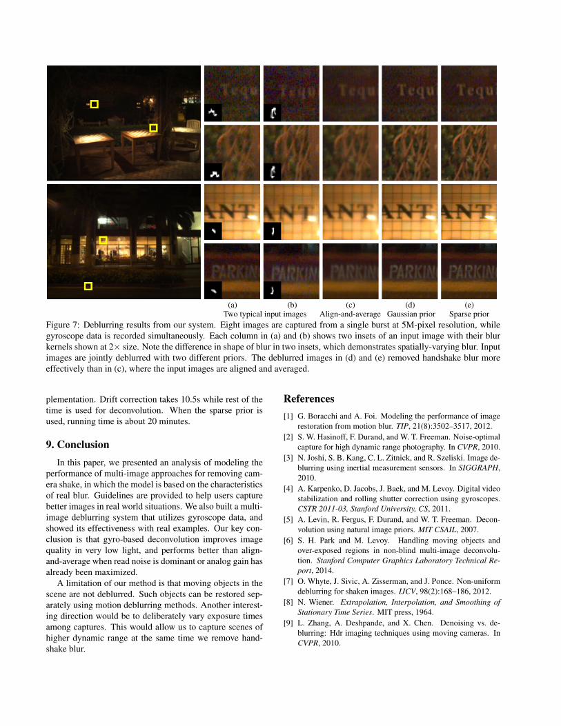
(a) (b) (c) (d) (e)Two typical input images Align-and-average Gaussian prior Sparse prior

Figure 7: Deblurring results from our system. Eight images are captured from a single burst at 5M-pixel resolution, whilegyroscope data is recorded simultaneously. Each column in (a) and (b) shows two insets of an input image with their blurkernels shown at 2× size. Note the difference in shape of blur in two insets, which demonstrates spatially-varying blur. Inputimages are jointly deblurred with two different priors. The deblurred images in (d) and (e) removed handshake blur moreeffectively than in (c), where the input images are aligned and averaged.

plementation. Drift correction takes 10.5s while rest of thetime is used for deconvolution. When the sparse prior isused, running time is about 20 minutes.

9. ConclusionIn this paper, we presented an analysis of modeling the

performance of multi-image approaches for removing cam-era shake, in which the model is based on the characteristicsof real blur. Guidelines are provided to help users capturebetter images in real world situations. We also built a multi-image deblurring system that utilizes gyroscope data, andshowed its effectiveness with real examples. Our key con-clusion is that gyro-based deconvolution improves imagequality in very low light, and performs better than align-and-average when read noise is dominant or analog gain hasalready been maximized.

A limitation of our method is that moving objects in thescene are not deblurred. Such objects can be restored sep-arately using motion deblurring methods. Another interest-ing direction would be to deliberately vary exposure timesamong captures. This would allow us to capture scenes ofhigher dynamic range at the same time we remove hand-shake blur.

References[1] G. Boracchi and A. Foi. Modeling the performance of image

restoration from motion blur. TIP, 21(8):3502–3517, 2012.[2] S. W. Hasinoff, F. Durand, and W. T. Freeman. Noise-optimal

capture for high dynamic range photography. In CVPR, 2010.[3] N. Joshi, S. B. Kang, C. L. Zitnick, and R. Szeliski. Image de-

blurring using inertial measurement sensors. In SIGGRAPH,2010.

[4] A. Karpenko, D. Jacobs, J. Baek, and M. Levoy. Digital videostabilization and rolling shutter correction using gyroscopes.CSTR 2011-03, Stanford University, CS, 2011.

[5] A. Levin, R. Fergus, F. Durand, and W. T. Freeman. Decon-volution using natural image priors. MIT CSAIL, 2007.

[6] S. H. Park and M. Levoy. Handling moving objects andover-exposed regions in non-blind multi-image deconvolu-tion. Stanford Computer Graphics Laboratory Technical Re-port, 2014.

[7] O. Whyte, J. Sivic, A. Zisserman, and J. Ponce. Non-uniformdeblurring for shaken images. IJCV, 98(2):168–186, 2012.

[8] N. Wiener. Extrapolation, Interpolation, and Smoothing ofStationary Time Series. MIT press, 1964.

[9] L. Zhang, A. Deshpande, and X. Chen. Denoising vs. de-blurring: Hdr imaging techniques using moving cameras. InCVPR, 2010.