gurievkvassovfinal - purdue university
TRANSCRIPT

BARTER FOR PRICE DISCRIMINATION
Sergei Guriev∗and Dmitri Kvassov†
February 2003
Abstract
We study barter as a discriminatory instrument in oligopoly with asymmetric infor-
mation. Buyers (producers of final goods) differ in the quality of their products. Sellers
(producers of inputs) use barter as a screening device: the higher quality buyers pay
in cash while the lower quality ones pay in kind. Barter, identified with non-monetary
contracts that give a seller control over a buyer’s output, emerges in equilibrium even
in the absence of financial constraints.
There is a positive relationship between market concentration and the level of
barter. Barter disappears as the market becomes more competitive. Barter and no-
barter equilibria coexist for a range of market structures.
JEL Codes: D43, L13, P42.
Keywords: barter, price discrimination, oligopoly.
∗New Economic School, CEFIR, CEPR and WDI. Address: New Economic School, Nakhimovsky pr. 47,
Moscow 117418 Russia. Tel. (7-095) 129-3911. Fax: (7-095) 129-3722. E-mail: [email protected].
†Pennsylvania State University. E-mail: [email protected]
1

1 Introduction
Monetary economics predicts that money should crowd out barter as a medium of exchange.
The superiority of money is established in various general equilibrium settings with asym-
metric information and/or random matching (e.g. Kiyotaki and Wright, 1989, Banerjee and
Maskin, 1996). However, barter continues to be used in the trade between OECD and de-
veloping economies (Marin and Schnitzer, 1996) and is growing within OECD economies.
The barter exchanges in the US reached a value of 10 billion dollars in 1998 (Economist,
2000). Moreover, in several transition economies barter has effectively overtaken money as
the major means of exchange in the second half of 1990s; barter accounted for 30 to 70
percent of inter-firm transactions in Russia (Aukutzionek, 1998, Seabright, 2000).1
The International Reciprocal Trade Association, the leading association of barter com-
panies in OECD countries, offers (IRTA, 2001) two common sense explanations of barter:
(i) financial constraints: ‘barter is a relatively inexpensive method of finance’, and (ii) spare
capacity: ‘to take advantage of barter, a firm must have slow-moving or non-performing
assets to exchange, or spare capacity to take on additional sales’. The former argument is
quite intuitive, the latter is less so. If a firm sells some of its goods for cash and the rest for
barter at different relative prices then the firm effectively engages in price discrimination. It
is not clear, however, why in order to discriminate firm has to use barter rather than cash
contracts (e.g. discounts on ‘slowly moving’ goods).
The paper presents a model of imperfect competition in which barter contracts indeed
enhance firm’s ability to price discriminate. The argument is based on asymmetric informa-
tion: the quality of the good involved in barter payments is better known to its producer.
Barter contracts may, therefore, be used as a screening device. The firms that produce out-
put of higher quality prefer to keep it and pay the supplier in cash while the firms with low
quality output keep cash and pay in kind. This self-selection, in turn, allows the supplier
to benefit from barter. Were there no barter, the volume of trade would be inefficiently low
due to imperfect competition; some customers willing to pay a price above the marginal cost
would not be served. Barter allows serving the lower quality customers without sacrificing
the profits from the high quality ones who prefer to pay in cash.
1In Banerjee and Maskin (1996) barter may prevail in an equilibrium with high inflation. In Russia,
however, the growth of barter was observed after the inflation was brought down.
2

The issue of barter as a price discriminatory device has been addressed in the literature.
Caves (1974) and Caves and Marin (1992) show that the price discrimination is responsible
for the widespread use of countertrade in trade between OECD and developing countries.2
The model in Caves (1974), however, is applicable only to international trade when cus-
tomers are exogenously separated and first or third-degree price discrimination is possible.
In contrast, this paper developes a model of second-degree price discrimination.
Prendergast and Stole (1998, 1999), Ellingsen (1998), and Marin and Schnitzer (1999)
show, in different settings, that barter emerges as a means of segmenting markets in the
presence of asymmetric information or contractual incompleteness, (bilateral) monopoly,
and liquidity constraints. The presence of liquidity constraints is crucial to all these models.
Ellingsen (1998) shows that barter helps to separate buyers whenever liquidity constraints
do not allow firms to discriminate through money. Prendergast and Stole (1998) prove that
in their setting barter emerges only in the presence of liquidity constraints. Marin and
Schnitzer (1999) explicitly refer to liquidity constraints as to one of the two major building
blocks of their model.
Our contribution to the existing literature is two-fold. First, we show that barter may
emerge as a means of price discrimination even if there are no liquidity constraints. Moreover,
to demonstrate that barter, even if it is extremely inefficient, can emerge in the presence of
market power we introduce additional costs of barter: lack of the double coincidence of wants
and imperfect divisibility. Second, we analyze partial equilibrium in the case of oligopoly
rather than monopoly. The analysis of strategic interaction among sellers does produce new
insights. Self-selection of buyers gives rise to the emergence of the ’cash demand externality’
that one seller’s choice imposes on the others. If a firm sells a greater share of its output for
cash, cash prices go down, and the most efficient barter customers switch to cash payments.
With these customers leaving the barter economy, the average quality of in-kind payments
deteriorates and the firm’s competitors have more incentives to sell for cash. The cash
demand externality leads to multiple equilibria which, in turn, may explain why barter has
been so widespread in Russia but not in the other countries.
The paper proceeds as follows. Section 2 lays out a model and examines equilibria in the
2Ellingsen and Stole (1996) suggest that international barter may act as a commitment device not to
engage in unilateral imports. Magenheim and Murrell (1988) put forward yet another reason to use barter
for price discrimination: in a repeated game, barter helps not to reveal the seller’s type to future customers.
3

cases of monopoly and oligopoly. Section 3 illustrates the theoretical findings using empirical
evidence on barter in Russia. Section 4 concludes.
2 The model
In this Section we study a model of barter as a screening device for price discrimination.
Subsection 2.1 starts with a standard model of monopoly serving a continuum of buyers.
Subsection 2.2 introduces barter contracts, Subsection 2.3 extends the analysis to the case
of oligopoly.
2.1 The setting
Monopoly seller S with the constant marginal costs of production c ∈ [0, 1] supplies an inputto a continuum of buyers (industrial firms). Each buyer B has access to a linear technology
with the maximum capacity of one unit which transforms q ∈ [0, 1] units of the input intoq units of output. Each unit of output is worth v to the buyer. B’s productivity (type) v
is her private information and is distributed on [0, 1] with a c.d.f. F (v). The distribution
function F (v) is common knowledge. B’s ex-ante outside option is zero.
The timing is as follows. The seller S offers a menu of contracts, each buyer B learns
her type v and chooses a contract, the contract is signed and input delivery occurs. Then
buyers produce output, and the quality of each buyer’s output v is observed by all agents.
The timing has two implications that are crucial for the following analysis. First, while
the buyer’s type is private information at the time of purchasing the input, it is revealed
later. Effectively, we assume that the type is realized during production, so that there is no
information asymmetry at the time of selling the output.
Second, the input cannot be resold by one buyer to another buyer: once purchased, it
can only be used in the production. This assumption is common for all price discrimination
models. It is related to the Myerson-Satterthwaite theorem: since at the time of potential
resale, the parties’ valuations of the input are private information, there arise transaction
costs in the secondary market. Also, there may be technological barriers to resale: e.g.
natural gas, electricity, heating, transportation (or other) services cannot be easily resold.
4
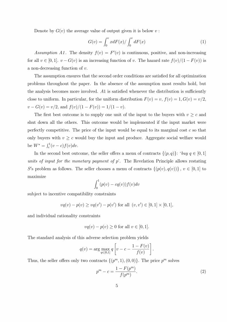
Denote by G(v) the average value of output given it is below v :
G(v) =Z v
0xdF (x)/
Z v
0dF (x) (1)
Assumption A1 . The density f(v) = F 0(v) is continuous, positive, and non-increasing
for all v ∈ [0, 1]. v−G(v) is an increasing function of v. The hazard rate f(v)/(1−F (v)) isa non-decreasing function of v.
The assumption ensures that the second order conditions are satisfied for all optimization
problems throughout the paper. In the absence of the assumption most results hold, but
the analysis becomes more involved. A1 is satisfied whenever the distribution is sufficiently
close to uniform. In particular, for the uniform distribution F (v) = v, f(v) = 1, G(v) = v/2,
v −G(v) = v/2, and f(v)/(1− F (v)) = 1/(1− v).The first best outcome is to supply one unit of the input to the buyers with v ≥ c and
shut down all the others. This outcome would be implemented if the input market were
perfectly competitive. The price of the input would be equal to its marginal cost c so that
only buyers with v ≥ c would buy the input and produce. Aggregate social welfare wouldbe W ∗ =
R 1c (v − c)f(v)dv.
In the second best outcome, the seller offers a menu of contracts {(p, q)}: ‘buy q ∈ [0, 1]units of input for the monetary payment of p’. The Revelation Principle allows restating
S0s problem as follows. The seller chooses a menu of contracts {(p(v), q(v))} , v ∈ [0, 1] tomaximize Z 1
0(p(v)− cq(v))f(v)dv
subject to incentive compatibility constraints
vq(v)− p(v) ≥ vq(v0)− p(v0) for all (v, v0) ∈ [0, 1]× [0, 1],
and individual rationality constraints
vq(v)− p(v) ≥ 0 for all v ∈ [0, 1].
The standard analysis of this adverse selection problem yields
q(v) = arg maxq∈[0,1]
q
"v − c− 1− F (v)
f(v)
#.
Thus, the seller offers only two contracts {(pm, 1), (0, 0)}. The price pm solves
pm − c = 1− F (pm)f(pm)
. (2)
5

Assumption A1 implies that pm ∈ [c, 1] is unique. Only buyers with v ≥ pm buy the inputand produce. The deadweight loss Z pm
c(v − c)f(v)dv (3)
results because buyers with v ∈ [c, pm), who could potentially add value, do not produce.
Remark 1 The equilibrium is essentially the textbook case of a non-discriminating monopoly
serving the market with the demand D(p) = 1 − F (p). Monopoly does not discriminate inequilibrium because both cost and utility are linear in quantity, and all agents are risk-neutral.
2.2 Barter as a means of price discrimination
To show that barter can emerge in the presence of market power, even if it is extremely
inefficient, we introduce all possible costs of barter. Liquidity constraints that may make
money inferior to barter are also not imposed.
The first drawback of barter is the need for the double coincidence of wants. We assume
that the seller values the buyer’s output less than the buyer herself. A unit of buyer v’s
product is worth only αv to the seller, where α ∈ (0, 1) . It implies that the seller hasan inferior technology for re-selling or using the buyer’s product, or there are storage or
transportation costs borne by the seller. The cost of barter 1−α may also be interpreted as
the probability that there is no double coincidence of wants and S has to throw the in-kind
payment away.
Another disadvantage of barter is that, unlike money, it is not perfectly divisible. For the
sake of simplicity, we assume the extreme degree of indivisibility and allow only contracts
with b ∈ {0, 1}. This assumption is a modelling shortcut for the increasing returns in thebarter exchange. The legal, storage, and transportation costs per unit of barter decrease with
the amount bartered, therefore, exchanging small portions of the good may be prohibitively
costly.
Suppose now that the seller can offer the buyers a menu of triplets {(p, b, q)}: ‘buyq ∈ [0, 1] units of input for the monetary payment of p and the in-kind payment b ≤ q’. Thelatter means that b out of q units produced are to be given back to the seller.
The timing is similar to that of Section 2.1 (see Figure 1). If buyer of type v chooses
contract (p, b, q) she gets v(q − b)− p and the seller gets p+ αvb− cq. Using the Revelation
6

S offers B a menu of contracts {(p,b,q)}
B chooses a contract (p,b,q) or leaves
B quits, game ends, everyone gets nil
Contract is executed. B gives S p dollars in cash and b units of output in kind.
Quality v is revealed to public. Output is sold for cash. B gets v(q-b), S gets αvb.
q units of input are delivered. S incurs cost cq. B produces q units of output.
B learns v
Figure 1: The timing of the game in Subsection 2.2 (also applies to Subsection 2.1 if b = 0).
Principle the problem is restated as follows: the monopolist chooses a menu of triplets
{(p(v), q(v), b(v))}, v ∈ [0, 1], b(v) ∈ {0, 1}, b(v) ≤ q(v) to maximizeZ 1
0(p(v) + αvb(v)− cq(v))f(v)dv (4)
subject to incentive compatibility constraints
v(q(v)− b(v))− p(v) ≥ v(q(v0)− b(v0))− p(v0) for all (v, v0) ∈ [0, 1]× [0, 1], (5)
and individual rationality constraints
v(q(v)− b(v))− p(v) ≥ 0 for all v ∈ [0, 1]. (6)
Denote by pmb and p∗ the solutions to
pmb(1− α) =1− F (pmb)f(pmb)
), (7)
and
αG(p∗) = c, (8)
respectively. Denote by c̄ the value of c that solves
pmb(1− F (pmb)) + αG(pmb)F (pmb)− c = (pm − c)(1− F (pm)). (9)
7

By definition, pmb, p∗ and c̄ are unique. Also, c̄ decreases with α : dc̄/dα = G(pmb)F (pmb)/F (pm) >
0, and c̄ goes to 0 as α approaches 0.
Lemma 1 and Proposition 1 below describe the structure of equilibria.
Lemma 1 If a menu of contracts {(p(v), b(v), q(v))}, v ∈ [0, 1], b(v) ∈ {0, 1}, b(v) ≤ q(v)satisfies the incentive compatibility (5) and participation constraints (6) then there exists
v̄ ∈ [0, 1] such that:(i) all buyers with v < v take the outside option or pay in kind;
(ii) all buyers with v > v pay in cash and q(v) is non-decreasing in v for all v ≥ v.
Proof. In the Appendix.
Proposition 1 The optimal menu of contracts is:
(a) if c > c̄, S does not use barter and offers the contracts {(pm, 0, 1), (0, 0, 0)};
(b) if c < c̄, S uses barter and offers the contracts {(pmb, 0, 1), (0, 1, 1), (0, 0, 0)};in this case, pmb > pm, and pmb > p∗.
Proof. In the Appendix.
In the rest of the subsection, we discuss the properties of and the intuition behind the
barter equilibrium, i.e. concentrate on the case c < c̄. When S chooses to use barter, the
buyers with the higher valuations v ≥ pmb pay in cash while all the buyers with the lowervaluations pay in kind. The ‘barter customers’ with the valuations v < c who should not be
served in the social optimum are pooled together with the efficient ones with the valuations
v ∈ (c, pmb). And, if the gap between cash price and marginal cost is sufficiently large,serving this pool of customers is profitable for the seller. The average quality of the output
is G(pmb). Since pmb > p∗, the in-kind revenues exceed marginal cost αG(pmb) > αG(p∗) = c,
and S receives positive profit from barter sales.
The condition c < c̄ also implies that in presence of barter contracts the cash price is
higher: pmb > pm. The intuition is simple: if there were no barter, increasing the monetary
price would result in losing customers, while in the presence of barter these customers do
not leave the market, they switch to paying in kind and, in fact, improve the average quality
of the barter payments.
8

Example. Consider a uniform distribution f(v) = 1. In this case c̄ = (1− α/2)−1/2 − 1,pmb = 1/(2− α), pm = (1 + c)/2, p∗ = 2c/α.
The welfare effect of barter is ambiguous. The deadweight loss in the equilibrium with
barter (1 − α)G(pmb)F (pmb) + (c − G(c))F (c) may be either larger or smaller than thedeadweight loss without barter (3). Were barter prohibited, the monopoly seller would
produce too little input, and some efficient buyers would close down. If, however, barter were
allowed, the losses are not only due to lack of the double coincidence of wants (proportional
to 1 − α), but also due to asymmetric information about the quality of in-kind payments.
The average value of barter payments is greater than the input cost but some of the barter
customers actually subtract value. This is the direct implication of the indivisibility of
barter. Were barter payments perfectly divisible, the seller would be able to discriminate
against inefficient buyers and only sell for barter to the buyers with v > c/α (see Proof of
Proposition 1).
Remark 2 The model above can also be applied to a pure exchange setting, where v and
αv are simply the values of a unit of the in-kind payments to the buyer and the seller,
respectively. In this case, second-degree price discrimination through barter also results if v
is the buyer’s private information.
Remark 3 The barter menu is similar to a standard debt contract with a privately known
value of the collateral. The debt contract states: ‘S supplies q unit of input to B, B pays back
pmb in cash else S gets ownership of B’s output’. Barter trade is essentially the (inefficient)
liquidation which destroys (1 − α) of the collateral’s value. Unlike the literature on debt
contracts, we assume that there is no ex-post renegotiation (or that the renegotiation is very
costly). The model with renegotiation, provided that the buyer has at least some bargaining
power, would have a very similar equilibrium, except the elimination of the deadweight loss
caused by the lack of double coincidence of wants.
2.3 Barter in oligopoly
Suppose there are N identical sellers with the marginal cost c. We study second-degree price
discrimination in the Cournot oligopoly setting assuming that sellers determine how much
to sell for cash and how much for barter taking into account the self-selection of buyers.
9

Each seller offers customers the following menu of contracts: a non-linear cash tariff
{p(q), 0, q} ‘buy q ∈ [0, 1] units of input and pay p(q) in cash’ and a barter contract (p, 1, 1)‘buy one unit of input and pay one unit of output and p in cash’. Each buyer compares three
options: (a) the outside option that gives zero payoff, (b) the barter contract that gives
U = −p, (c) the cash contract that gives U(v) = maxq∈[0,1] vq − p(q), and chooses one thatmaximizes her rent.
We define Cournot equilibrium in the way described in Oren et al. (1983) extending it
to the setting in which the sellers can use both cash and barter contracts. In the linear case,
as shown below, this model is reduced to a very simple game among the oligopolists.3
Denote by v∗(q) the highest type that buys q units of input and pays in cash. The
buyers’ choice is the same as in the previous section; hence Lemma 1 applies and v∗(q) is an
increasing function of q.
Each seller i is characterized by a function Ti(q) — the number of customers buying no
more than q units for cash from i. By definitionPNi=1 Ti(q) = F (v
∗(q)) for all q > 0. Ti(0)
is the number of customers buying from i for barter. Each seller takes Tj(q), j 6= i as givenand chooses p(q), p, and Ti(0) to maximize profit
(αG(v∗(0))− c)(F (v∗(0))− T−i(q))Ti(0)I(p ≥ 0) ++Z 1
0(p(q)− cq)d(F (v∗(q))− T−i(q)) (10)
subject to the constraint that v∗(q) is the inverse of the buyer’s optimal response to p(q),
p. Here T−i(q) =Pj 6=i Tj(q), and I(p ≥ 0) is the indicator function that equals 1 whenever
p ≥ 0 and is 0 otherwise. We look for symmetric equilibria where Ti(q) = Tj(q) for all i, j,and q.
Lemma 2 In any Cournot equilibrium, there are no buyers who buy q ∈ (0, 1) for cash.
Proof. In the Appendix.
Just as in the monopoly case, linear utility and cost functions rule out the intermediate
quantities. This makes the contract menu very simple, buyers choose among three options:
(i) buy one unit for cash; (ii) buy one unit for barter, (iii) do not buy at all.
3Ivaldi and Martimort (1994) and Stole (1995) model second-degree price discrimination under duopoly
with imperfect substitutes, but these models are too complicated to study comparative statics with regard
to change in the market structure.
10
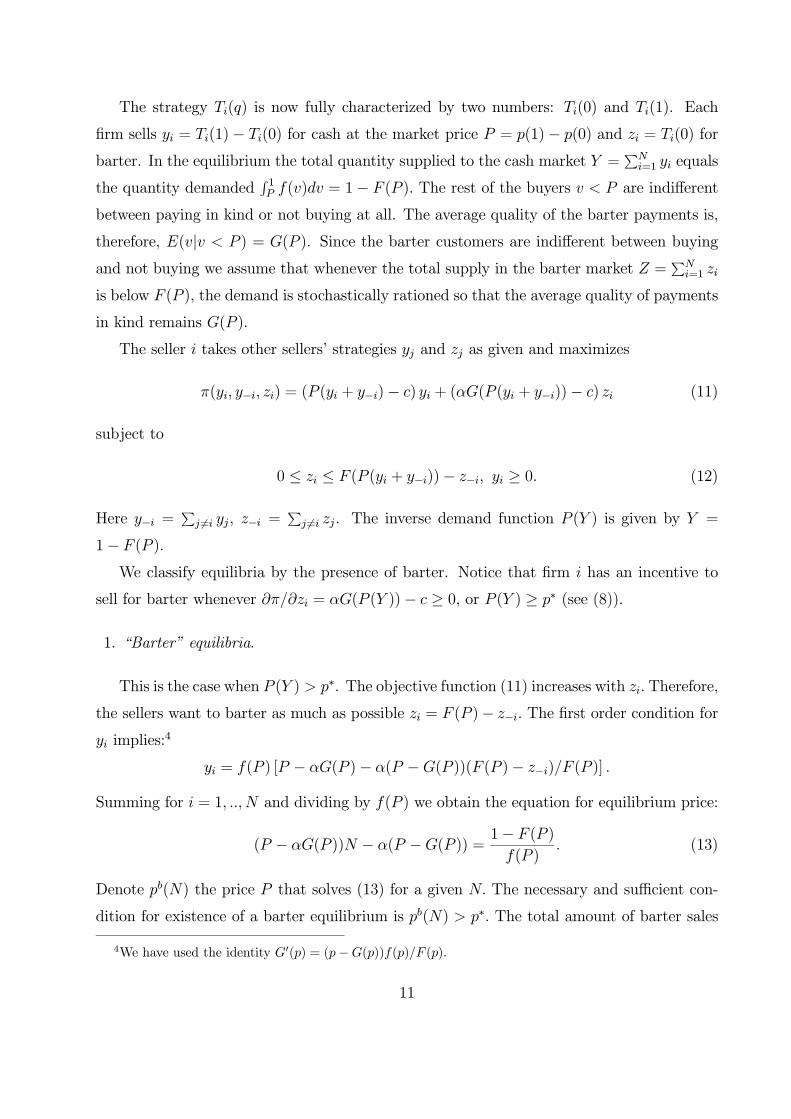
The strategy Ti(q) is now fully characterized by two numbers: Ti(0) and Ti(1). Each
firm sells yi = Ti(1)− Ti(0) for cash at the market price P = p(1)− p(0) and zi = Ti(0) forbarter. In the equilibrium the total quantity supplied to the cash market Y =
PNi=1 yi equals
the quantity demandedR 1P f(v)dv = 1− F (P ). The rest of the buyers v < P are indifferent
between paying in kind or not buying at all. The average quality of the barter payments is,
therefore, E(v|v < P ) = G(P ). Since the barter customers are indifferent between buyingand not buying we assume that whenever the total supply in the barter market Z =
PNi=1 zi
is below F (P ), the demand is stochastically rationed so that the average quality of payments
in kind remains G(P ).
The seller i takes other sellers’ strategies yj and zj as given and maximizes
π(yi, y−i, zi) = (P (yi + y−i)− c) yi + (αG(P (yi + y−i))− c) zi (11)
subject to
0 ≤ zi ≤ F (P (yi + y−i))− z−i, yi ≥ 0. (12)
Here y−i =Pj 6=i yj, z−i =
Pj 6=i zj. The inverse demand function P (Y ) is given by Y =
1− F (P ).We classify equilibria by the presence of barter. Notice that firm i has an incentive to
sell for barter whenever ∂π/∂zi = αG(P (Y ))− c ≥ 0, or P (Y ) ≥ p∗ (see (8)).
1. “Barter” equilibria.
This is the case when P (Y ) > p∗. The objective function (11) increases with zi. Therefore,
the sellers want to barter as much as possible zi = F (P )− z−i. The first order condition foryi implies:
4
yi = f(P ) [P − αG(P )− α(P −G(P ))(F (P )− z−i)/F (P )] .
Summing for i = 1, .., N and dividing by f(P ) we obtain the equation for equilibrium price:
(P − αG(P ))N − α(P −G(P )) = 1− F (P )f(P )
. (13)
Denote pb(N) the price P that solves (13) for a given N. The necessary and sufficient con-
dition for existence of a barter equilibrium is pb(N) > p∗. The total amount of barter sales
4We have used the identity G0(p) = (p−G(p))f(p)/F (p).
11
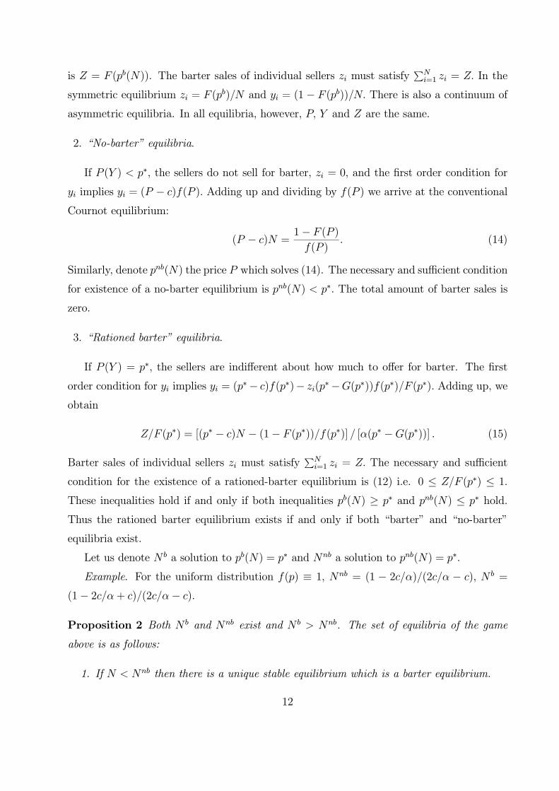
is Z = F (pb(N)). The barter sales of individual sellers zi must satisfyPNi=1 zi = Z. In the
symmetric equilibrium zi = F (pb)/N and yi = (1− F (pb))/N. There is also a continuum of
asymmetric equilibria. In all equilibria, however, P, Y and Z are the same.
2. “No-barter” equilibria.
If P (Y ) < p∗, the sellers do not sell for barter, zi = 0, and the first order condition for
yi implies yi = (P − c)f(P ). Adding up and dividing by f(P ) we arrive at the conventionalCournot equilibrium:
(P − c)N =1− F (P )f(P )
. (14)
Similarly, denote pnb(N) the price P which solves (14). The necessary and sufficient condition
for existence of a no-barter equilibrium is pnb(N) < p∗. The total amount of barter sales is
zero.
3. “Rationed barter” equilibria.
If P (Y ) = p∗, the sellers are indifferent about how much to offer for barter. The first
order condition for yi implies yi = (p∗− c)f(p∗)− zi(p∗−G(p∗))f(p∗)/F (p∗). Adding up, we
obtain
Z/F (p∗) = [(p∗ − c)N − (1− F (p∗))/f(p∗)] / [α(p∗ −G(p∗))] . (15)
Barter sales of individual sellers zi must satisfyPNi=1 zi = Z. The necessary and sufficient
condition for the existence of a rationed-barter equilibrium is (12) i.e. 0 ≤ Z/F (p∗) ≤ 1.These inequalities hold if and only if both inequalities pb(N) ≥ p∗ and pnb(N) ≤ p∗ hold.Thus the rationed barter equilibrium exists if and only if both “barter” and “no-barter”
equilibria exist.
Let us denote N b a solution to pb(N) = p∗ and Nnb a solution to pnb(N) = p∗.
Example. For the uniform distribution f(p) ≡ 1, Nnb = (1 − 2c/α)/(2c/α − c), N b =
(1− 2c/α+ c)/(2c/α− c).
Proposition 2 Both N b and Nnb exist and N b > Nnb. The set of equilibria of the game
above is as follows:
1. If N < Nnb then there is a unique stable equilibrium which is a barter equilibrium.
12

pnb(N)
p*
N bN nb N0
p
pb(N)
Figure 2: Oligopoly price P as a function of the number of sellers N.
2. If N > N b then there is a unique stable equilibrium which is a no-barter equilibrium.
3. If N ∈ (Nnb, N b) then there are three equilibria two of which (barter and no-barter)
are stable and one (rationed barter) is unstable.
4. If N = N b then there are two equilibria: a stable one (no-barter) and an unstable one
(rationed barter).
5. If N = Nnb then there are two equilibria: a stable one (barter) and an unstable one
(rationed barter).
Proof. In the Appendix.
Figure 2 illustrates the structure of equilibria according to Proposition 2.
The intuition for the multiplicity of equilibria at N ∈ (Nnb, N b) is as follows. Whenever
one seller chooses to sell more for cash, she drives down the cash price of the input. The
13

Barter equilibria
B
0 Nnb Nb N
F(p*)
Rationed-barter equilibria
No-barter equilibria
Figure 3: Share of barter sales in total sales B = Z/(Z + Y ) as a function of the number of
sellers N.
additional cash purchases are made by buyers who were the most efficient ones among those
paying in kind. With these buyers switching from barter to cash, the average quality of
payments in kind decreases. The other sellers will, therefore, have incentives to sell more for
cash and less for barter as well.
The comparative statics with respect to market structure (total number of sellers N)
are quite intuitive. First, in both barter and no-barter equilibria prices decrease as the
number of sellers increases. Second, given market structure the cash price in the barter
equilibrium is always greater than in the no-barter equilibrium. In barter equilibria, sellers
charge higher prices because the marginal buyer, who would leave the market were there no
barter, switches to barter and, therefore, contributes to profits from barter sales. Third, in
the barter equilibria the cash price should be above a certain level p∗; otherwise the average
14
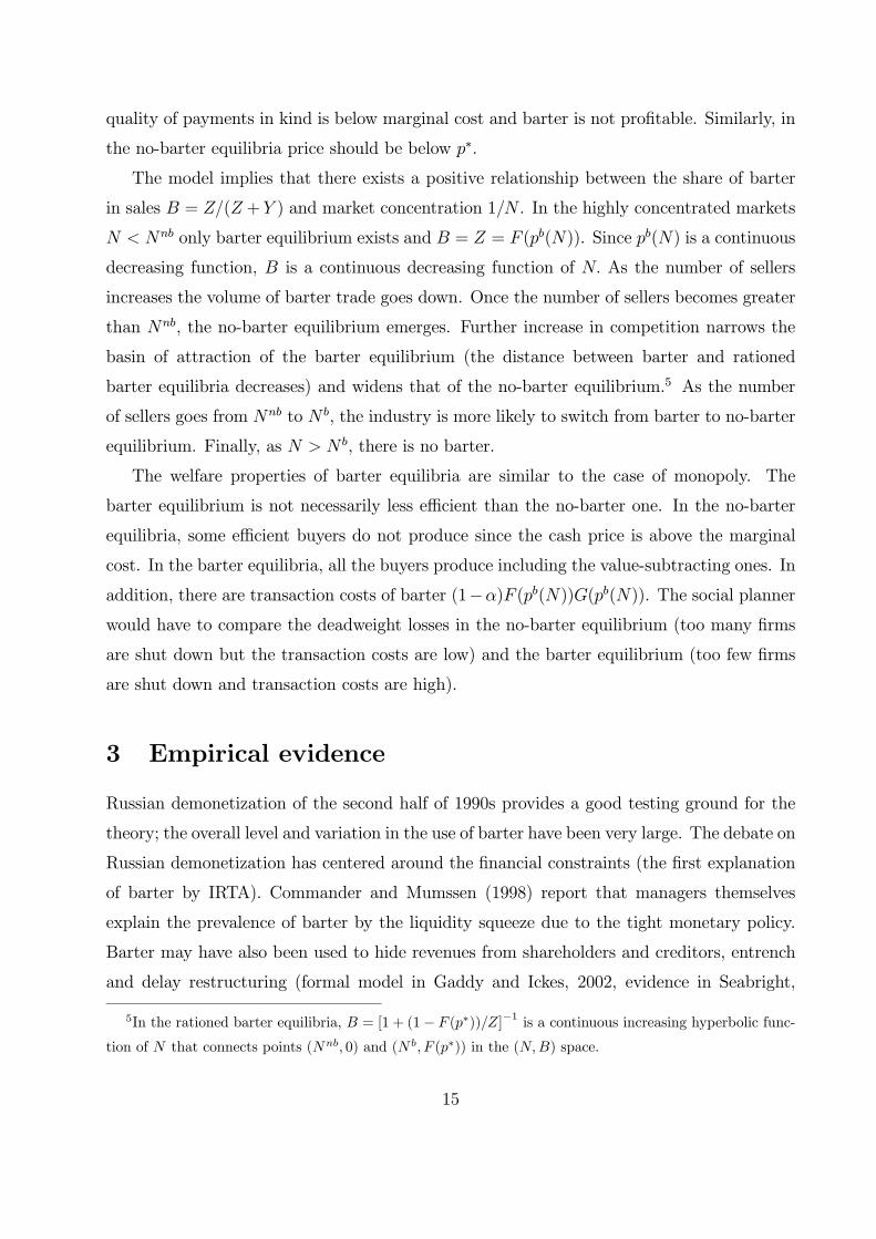
quality of payments in kind is below marginal cost and barter is not profitable. Similarly, in
the no-barter equilibria price should be below p∗.
The model implies that there exists a positive relationship between the share of barter
in sales B = Z/(Z +Y ) and market concentration 1/N . In the highly concentrated markets
N < Nnb only barter equilibrium exists and B = Z = F (pb(N)). Since pb(N) is a continuous
decreasing function, B is a continuous decreasing function of N. As the number of sellers
increases the volume of barter trade goes down. Once the number of sellers becomes greater
than Nnb, the no-barter equilibrium emerges. Further increase in competition narrows the
basin of attraction of the barter equilibrium (the distance between barter and rationed
barter equilibria decreases) and widens that of the no-barter equilibrium.5 As the number
of sellers goes from Nnb to N b, the industry is more likely to switch from barter to no-barter
equilibrium. Finally, as N > N b, there is no barter.
The welfare properties of barter equilibria are similar to the case of monopoly. The
barter equilibrium is not necessarily less efficient than the no-barter one. In the no-barter
equilibria, some efficient buyers do not produce since the cash price is above the marginal
cost. In the barter equilibria, all the buyers produce including the value-subtracting ones. In
addition, there are transaction costs of barter (1−α)F (pb(N))G(pb(N)). The social planner
would have to compare the deadweight losses in the no-barter equilibrium (too many firms
are shut down but the transaction costs are low) and the barter equilibrium (too few firms
are shut down and transaction costs are high).
3 Empirical evidence
Russian demonetization of the second half of 1990s provides a good testing ground for the
theory; the overall level and variation in the use of barter have been very large. The debate on
Russian demonetization has centered around the financial constraints (the first explanation
of barter by IRTA). Commander and Mumssen (1998) report that managers themselves
explain the prevalence of barter by the liquidity squeeze due to the tight monetary policy.
Barter may have also been used to hide revenues from shareholders and creditors, entrench
and delay restructuring (formal model in Gaddy and Ickes, 2002, evidence in Seabright,
5In the rationed barter equilibria, B = [1 + (1− F (p∗))/Z]−1 is a continuous increasing hyperbolic func-tion of N that connects points (Nnb, 0) and (N b, F (p∗)) in the (N,B) space.
15

2000, ch. 6 and 9). Other explanations include inefficiency of Russian fiscal federalism and
the inability of the federal government to enforce the monopoly to issue money (Woodruff,
1999).
This paper argues that the spread of barter in Russia may also be related to the second
motive for barter as suggested by IRTA (‘spare capacities’). The model predicts that barter
is more likely to occur in concentrated industries and decreases with competition. The
evidence on barter in Russia seems to be consistent with this prediction. It is the natural
monopolies that are engaged in barter the most (Gaddy and Ickes, 2002, Commander et
al., 2002). In 1996-97, Gazprom (the natural gas monopoly) and Unified Energy Systems
(the electricity monopoly) reported cash receipts of as low as 15 to 20 percent total revenue
(Pinto et al., 2000). The remainder of their revenues came in promissory notes, coal, metal,
machinery and even jet fighters. All case studies discussed in Woodruff (1999) refer to firms
that are either national or regional monopolies.
While it is hard to argue that the Russian demonetization was caused by price discrim-
ination, it turns out that the cross-sectional variation in the level of barter is related to
market power. Below we use a unique firm-level dataset to show that even controlling for
the common explanations the level of barter is indeed higher in more concentrated indus-
tries. The variation of barter across Russian industries in the mid-1990s is therefore generally
consistent with the above model of barter as a means of price discrimination.
3.1 Data and methodology
The empirical analysis uses three data sets: (i) surveys of managers of Russian industrial
firms conducted since 1996 by Serguei Tsoukhlo at the Institute of Economies in Transition,
Moscow;6 (ii) the database of financial accounts of industrial firms compiled by Goskomstat
(federal statistics agency); (iii) the Import Penetration Database compiled by the Russian
European Center for Economic Policy.
The dependent variable B (the share of barter in sales) comes from the firm manager’s
answers to the question: “what share of your firm’s sales was paid in kind?” The survey also
included questions on the other means of payment, our variable covers barter only (excluding
promissory notes). The average share of barter in sales is 39% and varies substantially across
6See Russian Business Survey Bulletin (1996) for a detailed description of the survey.
16

firms. It is distributed almost uniformly between 0 and 0.83. Only 10% of the sample have
the share of barter in sales lower than 5%.
Our main independent variables are the concentration ratio CR4 (the share of the four
largest firms in total sales of an industry) and import-adjusted concentration ratio CR4ia =
CR4 ∗ (1 − imp), where imp is the import penetration ratio. The ratios are calculated for5-digit industries (rough equivalent of US 4-digit industries). In the sample, 120 (out of 450)
industries are represented with 2.8 firms in each industry on average, with up to 19 firms in
some industries.
The relationship between market concentration and barter may also be explained by
transaction costs of barter (1 − α in terms of the model). First, per unit search, trans-
portation, and storage costs may be smaller for larger firms. At the same time, market
concentration is correlated with the average size of a firm in the industry. We control for
size by adding the variable SIZE (the logarithm of annual sales in denominated rubles).
Second, transaction costs of barter are prohibitively high for retail customers. Hence, in
consumer good industries, one should expect less barter. Also, these industries may be more
competitive. Thus, the correlation between barter and market power may be explained by
the lower level of barter in consumer good industries. To control for this effect, we introduce
a dummy for consumer good industries CGI.
Third, the fewer players in the market for buyers’ output, the lower the search costs of
barter. Certainly, the numbers of players in the markets for the input and for the buyers’
outputs may be correlated. This problem would be resolved via a panel regression, testing if
an increase in concentration in the seller’s market raises barter controlling for concentration
in the buyers’ markets. Unfortunately, the data on buyers are not available, and the dataset
is limited to one year. As an imperfect substitute, we use eleven broad industry dummies
— for the firms in the same broad industry, buyers are roughly the same. Also, the broad
industry dummies help to control for technological characteristics that can influence costs of
barter (e.g. per unit transportation costs). A similar role is played by regional dummies for
Moscow and seven federal districts (Central Russia, South, North-West, Volga, Ural, Siberia
and Far East). The base category is Central Russia excluding Moscow.
We also control for other determinants of barter. First, to measure firm liquidity, we
add the variable CASH — the ratio of stock of liquid assets (cash plus current accounts)
to annual sales. Second, the variable EXPORT (the share of exports in sales) controls for
17
sales to foreign customers.
The descriptive statistics and the correlation matrix are reported in Appendix B. The
signs of pairwise correlations are intuitive. There is indeed more barter in more concentrated
industries (whether adjusted for imports or not), in larger firms, and in those which sell less to
foreign customers and consumers. Consumer goods industries are less concentrated. Average
CR4 for consumer goods industries is 23 per cent which is significantly lower than in the
other industries (44 per cent). Liquidity is not correlated with barter, or other variables
except exports (exporting firms have more cash).
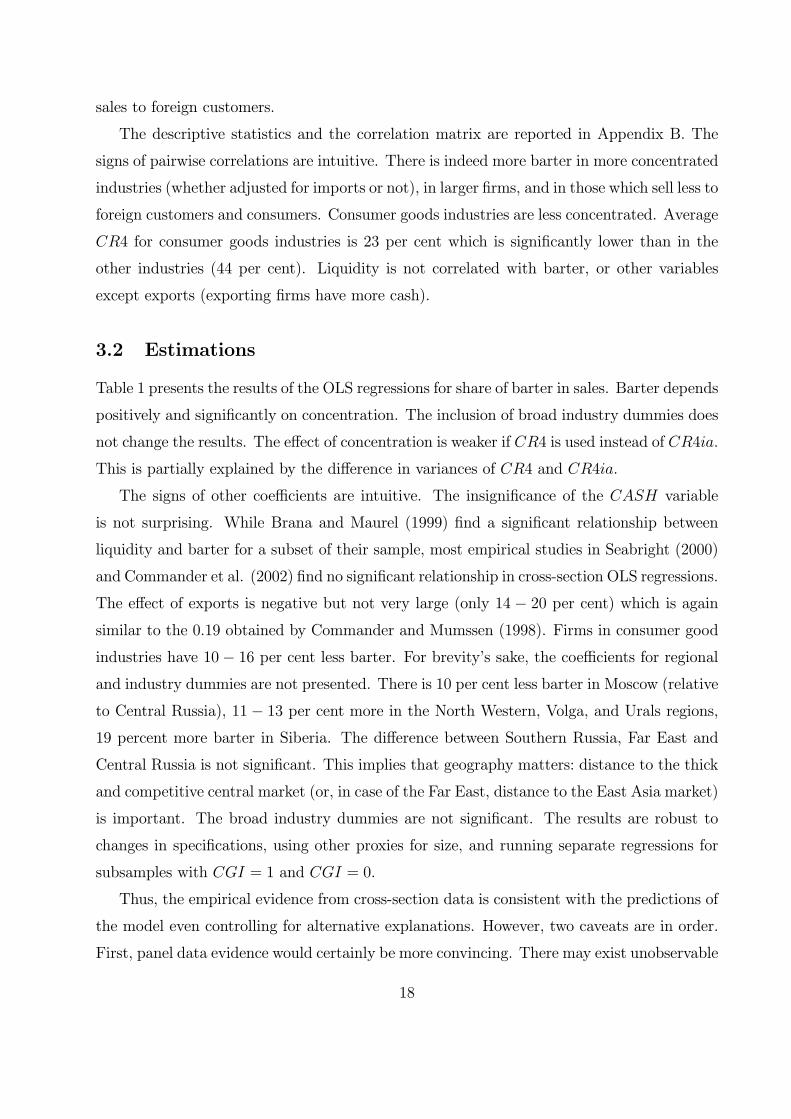
3.2 Estimations
Table 1 presents the results of the OLS regressions for share of barter in sales. Barter depends
positively and significantly on concentration. The inclusion of broad industry dummies does
not change the results. The effect of concentration is weaker if CR4 is used instead of CR4ia.
This is partially explained by the difference in variances of CR4 and CR4ia.
The signs of other coefficients are intuitive. The insignificance of the CASH variable
is not surprising. While Brana and Maurel (1999) find a significant relationship between
liquidity and barter for a subset of their sample, most empirical studies in Seabright (2000)
and Commander et al. (2002) find no significant relationship in cross-section OLS regressions.
The effect of exports is negative but not very large (only 14 − 20 per cent) which is againsimilar to the 0.19 obtained by Commander and Mumssen (1998). Firms in consumer good
industries have 10− 16 per cent less barter. For brevity’s sake, the coefficients for regionaland industry dummies are not presented. There is 10 per cent less barter in Moscow (relative
to Central Russia), 11− 13 per cent more in the North Western, Volga, and Urals regions,19 percent more barter in Siberia. The difference between Southern Russia, Far East and
Central Russia is not significant. This implies that geography matters: distance to the thick
and competitive central market (or, in case of the Far East, distance to the East Asia market)
is important. The broad industry dummies are not significant. The results are robust to
changes in specifications, using other proxies for size, and running separate regressions for
subsamples with CGI = 1 and CGI = 0.
Thus, the empirical evidence from cross-section data is consistent with the predictions of
the model even controlling for alternative explanations. However, two caveats are in order.
First, panel data evidence would certainly be more convincing. There may exist unobservable
18

Table 1 Results of OLS estimation for the share of barter in sales B.
Regression with CR4ia, industry dummies are not
included
Regression with CR4ia, industry
dummies are included
Regression with CR4, industry
dummies are not included
Regression with CR4, industry dummies are
included
CR4ia 0.22** (2.59)
0.23** (2.31) - -
CR4 - - 0.13** (2.05)
0.12** (1.97)
SIZE -0.006 (0.53)
0.002 (0.21)
-0.006 (0.55)
0.002 (0.19)
CGI -0.16*** (4.74)
-0.11*** (2.97)
-0.16*** (4.66)
-0.10*** (2.91)
CASH -0.04 (0.56)
-0.03 (0.53)
-0.04 (0.54)
-0.03 (0.52)
EXPORT -0.14** (2.33)
-0.19*** (3.03)
-0.15** (2.41)
-0.20 (3.12)
Regional dummies *** *** *** ***
Industry dummies - * - *
CONST 0.45*** (2.75)
0.32* (1.90)
0.25*** (2.67)
0.32* (1.90)
N 337 337 337 337
R2 0.29 0.33 0.28 0.32
Standard errors are estimated via the Huber-White procedure taking into account unobserved correlations within 5-digit industries ***, **, * Significant at the 1, 5, and 10% significance level, respectively
Figure 4:
19

firm-specific characteristics that influence willingness to barter (e.g. managers’ “relational
capital”, Gaddy and Ickes, 2002). To make a strong empirical argument, one would have
to prove that even controlling for the firm’s fixed or random effects, change in competition
leads to change in barter. The available data, however, do not allow us to perform this test.
Second, the model predicts that the relationship between barter and market concentration
may be non-linear. Elsewhere (Guriev and Kvassov, 2000) we tested for a structural break
and identified it at CR4 = 0.162 (or at CR4ia = 0.103). The nature of the structural break
is consistent with the model. For the industries with concentration above the threshold level
competition reduces barter, the coefficient is significant but relatively small (in the range of
0.1). Once concentration is below the threshold, barter starts to fall rapidly with further
increase in competition (coefficient becomes ten times as large): firms switch from barter
equilibria to ones without barter.
4 Concluding remarks
This paper shows that barter may be used as a discriminatory instrument in sufficiently con-
centrated markets with assymetric information. Imperfect competition is characterized by
underproduction relative to the social optimum. The sellers, therefore, are willing to employ
an additional channel of sales (barter) even if this channel is costly. The paper also demon-
strates that there exists a relationship between the share of barter in sales and the market
concentration. The only equilibrium at high levels of concentration is the barter equilibrium,
and the only equilibrium at low levels of concentration is the no-barter equilibrium. Barter
and no-barter equilibria coexist in the intermediate range of market concentration.
It is important to note that the model provides no clear ranking of the equilibria in terms
of social welfare. The equilibrium without barter is characterized by underproduction, many
efficient firms close down. In the barter equilibrium, on the other hand, all efficient firms
produce but so do inefficient ones; besides, barter involves high transaction costs. The paper
demonstrates that competition reduces barter and identifies the trade-offs this reduction
involves.
A number of simplifying assumptions were made to keep the model tractable. We have
assumed linear technology, risk neutrality, exogenous probability of double coincidence of
wants, perfect substitution of oligopolists’ products, extreme indivisibility of barter, etc.
20

However, the model is robust to relaxing these assumptions: introduction of convex technol-
ogy, for example, would result in price discrimination both with and without barter. But
barter still represents an additional dimension for price discrimination and would, therefore,
be used, only the equilibrium contracts become more complicated. This suggests that the
insights of the model are not confined to the question of barter in transition or developing
economics, but shed some new light on the theories of price discrimination under imperfect
competition in general.
It is also worth emphasizing that throughout the paper term ‘barter’ is used as a short-
hand for any non-monetary contract that involves the exchange of property rights. Thus, the
developed model may be used to analyse such diverse phenomena as the debt contracting
with asymmetric information about the value of collateral, or lease contracts where unob-
served actions of one party change the value of the good for the other party.
21

Acknowledgments
This work was part of the Research Project “Non-Monetary Transactions in Russian Econ-
omy” carried out in the New Economic School Research Center with the financial support
from Ford Foundation. We thank Sergei Golovan for excellent research assistance. We thank
Evgenia Bessonova, David Brown and Serguei Tsoukhlo for providing data. We are grateful
to Barry Ickes, Yulia Kossykh, Stephen Martin, Mathilde Maurel, Dominique Redor, Andrei
Sarychev, Mark Schaffer, Judith Shapiro, Giovanni Urga, Ekaterina Zhuravskaya, and two
anonymous referees, participants of the GET conference, WDI-CEPR Annual Conference
on Transition Economics, the World Congress of the Econometric Society, EARIE 2001,
seminar participants at NES, RECEP and ROSES, and colleagues at NES and CEFIR for
helpful comments.
22

Appendix A: Proofs
Proof of Lemma 1. Adding up the IC constraints (5)
v00(q(v00)− b(v00))− p(v00) ≥ v00(q(v0)− b(v0))− p(v0),v0(q(v0)− b(v0))− p(v0) ≥ v0(q(v00)− b(v00))− p(v00).
for arbitrary (v0, v00) ∈ [0, 1]× [0, 1] such that v0 < v00 yields
(v00 − v0) {(q(v00)− b(v00))− (q(v0)− b(v0))} ≥ 0.
Therefore, v00 > v0 implies that q(v00)− b(v00) ≥ q(v0)− b(v0). In other words, the amountof output kept by the buyer q(v)− b(v) is a monotonic function of v.Because only barter contracts with b(v) ∈ {0, 1} and b(v) ≤ q(v) are allowed, q(v)−b(v) =
0 for the buyers who pay in cash and for the buyers who exercise outside option. For the
buyers who pay in cash q(v)− b(v) equals q(v) > 0. Hence, there exists v such that buyerswith v < v pay in kind (or stay out), and buyers with v > v pay in cash. Moreover, since
b(v) = 0 for the buyers who pay in cash, q(v) is monotone non-decreasing function of v for
all v ≥ v.Proof of Proposition 1. S may offer a menu of cash contracts (p, q, 0) and one barter
contract (p, 1, 1). The buyer of type v gets the rent U(v) = v(q(v) − b(v)) − p(v). Con-sider arbitrary (v0, v00) ∈ [0, 1] × [0, 1] such that v0 < v00. From the incentive compatibility
constraints (5) it follows that
q(v0)− b(v0) ≤ U(v00)− U(v0)v00 − v0 ≤ q(v00)− b(v00).
Since q(v)− b(v) is monotonic in v (Lemma 1), integration yields
U(v) = U(0) +Z v
0[q(x)− b(x)] dx. (16)
Buyers who choose the barter contract get −p. They will prefer it to the outside option ifand only if p ≤ 0. The case with p > 0 (barter contract is proposed but is not chosen by anybuyer) is equivalent to the model without barter and the optimal menu is {(pm, 0, 1), (0, 0, 0)}.Payoff to the seller is the seller is (pm − c)(1− F (pm)). If the seller offers a barter contractwith p ≤ 0, then all buyers with v < v choose this contract and get U(v) = −p.
23

Using (16) andR 1v f(v)dv
R vv q(x)dx =
R 1v (1 − F (v))q(v)dv, S’s problem is restated as
follows. Seller chooses p ≤ 0, v ∈ (0, 1], and q(v) ∈ [0, 1] to maximize
p+Z v
0[αv − c] f(v)dv +
Z 1
v
Ãv − c− 1− F (v)
f(v)
!q(v)f(v)dv.
In the optimum, S sets p equal to zero and chooses
q(v) = arg maxq∈[0,1]
q
Ãv − c− 1− F (v)
f(v)
!for all v > v
where v maximizes
Π(v) = (αG(v)− c)F (v) + (max{v, pm}− c)(1− F (max{v, pm})) (17)
If v < pm then dΠ/dv = (αv − c) f (v) > 0 whenever v > c/α. If v > pm then
dΠ/dv = 1 − F (v) − (1− α) vf (v) > 0 whenever v < pmb. Assumption A1 implies that
pm is always between c/α and pmb. Indeed, pm > pmb is equivalent to (1− F (pm))/f(pm) <(1−F (pmb))/f(pmb) and, therefore, pm−c < pmb(1−α) < pm(1−α) which implies pm < c/α.Similar argument proves that pm < pmb implies pm > c/α. Therefore, the maximizer of (17)
is either v = 0 or v = pmb with the latter possible only if c/α < pm < pmb and the payoff to
the seller is pmb(1− F (pmb)) + αG(pmb)F (pmb)− c.Hence, the optimal menu of contracts is either {(pmb, 0, 1), (0, 1, 1), (0, 0, 0)} or {(pm, 0, 1),
(0, 0, 0)} whichever provides the seller with a higher payoff. The seller chooses to use barterif the left-hand side in (9) is greater than the right-hand side, which is the case whenever
c < c̄. Indeed, the left-hand side falls with c faster than the right-hand side.
Let us now prove that c < c̄ implies pmb > p∗. Since the left-hand side of (9) is greater
than the right-hand side,
(pmb − c)(1− F (pmb)) + (αG(pmb)− c)F (pmb) = maxp∈[0,1]
[p(1− F (p)) + αG(p)F (p)]− c >maxp{(p− c)(1− F (p))} ≥ (pmb − c)(1− F (pmb)).
Therefore, αG(pmb)− c > 0, and pmb > p∗.Comment. If barter were perfectly divisible b(v) ∈ [0, 1], the solution would be somewhat
different. If pmb < pm the equilibrium coincides with the monopoly equilibrium without
barter. If pmb > pm the seller is able to sort customers into three groups. The most efficient
buyers pay cash price pmb, the buyers with intermediate productivity v ∈ (c/α, pmb) pay in
24

kind, and the rest of buyers is not served. In this equilibrium all buyers with v ≤ pmb receivezero rent and are indifferent between paying in kind or not producing at all. Above, we
assumed that whenever indifferent, buyers choose to produce. To make buyers with v < c/α
shut down and buyers with v > c/α produce, the seller offers some infinitesimal reward to the
latter (1− b(v) strictly positive but very small). Although in equilibrium b(v) is either 0 or
very close to 1, perfect divisibility of barter is crucial for separating buyers with v ∈ (0, c/α)and v ∈ (c/α, pmb).Proof of Lemma 2. The seller maximizes (10) by choosing three scalar numbers
Ti(0), p, p(0) and a function p0(q) = dp/dq, q ∈ [0, 1]. The optimal choice of p0(q) does not
allow for intermediate purchases q ∈ (0, 1) for cash. Indeed, integration of the second termin (10) by parts yields
p(0)(1− T−i(q)− F (v∗(0)) + T−i(0)) +Z q
0(p0(q)− c)(1− T−i(q)− F (v∗(q)) + T−i(q))dq
where q is the quantity chosen by the buyers of the highest type v = 1.
The first term in (10) does not depend on p0(q), q ∈ (0, 1). Therefore, the seller choosesp0(q) to maximize Z q
0[p0(q)− c)(1− T−i(q)− F (v∗(q)) + T−i(q)] dq. (18)
Buyers choose q solving maxq∈[0,1] vq − p(q). Assume that there exist buyers that buy q ∈(0, 1) for cash. Then the first-order condition must hold v = p0(q). Substituting v∗(q) = p0(q)
into (18) we find p0(q) = ξ∗(q) = argmaxξ(ξ− c)(1−T−i(q)−F (ξ)+T−i(q)). The first-ordercondition is (ξ∗ − c)f(ξ∗) = 1 − T−i(q) − F (ξ∗) + T−i(q). Using the symmetry conditionTi(q) = Tj(q) =
1N−1T−i(q) =
1NF (v∗(q)) we obtain
ξ∗ − c = 1− F (ξ∗)Nf(ξ∗)
.
Assumption A1 implies that such ξ∗ exists and unique. It is crucial that ξ∗ is the same for
all q. Since p0(q) = ξ∗, the tariff is linear: p(q) = p(0)+ξ∗q. Therefore, all buyers with v < ξ∗
choose not to buy at all and all buyers with v > ξ∗ buy one unit (q = 1) . The set of buyers
who are indifferent v = ξ∗ is of measure zero.
Proof of Proposition 2. The proof consists of four steps.
Step 1. pb(N) and pnb(N) are decreasing functions of N and pb(N) > pnb(N) for all
N < N b.
25

Solving (13) for N we obtain
N = 1 + [(1− F (P ))/f(P )− (1− α)P ] / [P − αG(P )] (19)
which is a decreasing function of P . Consequently, the inverse function pb(N) is also decreas-
ing. Since pb(1) = pmb > p∗ and pb(∞) = 0, there exists a unique solution to pb(N) = p∗.Similarly, (14) implies N = (1−F (P ))/ [(P − c)f(P )] which is a decreasing function. Sincepnb(0) = 1 > p∗ and pb(∞) = c < p∗ there exists a unique solution to pnb(N) = p∗.For all N < N b, we have pb(N) > p∗ and therefore αG(pnb(N)) > c. Using (13) and (14)
for every N holds
1
N=(pnb − c)f(pnb)1− F (pnb) =
(pb − c)f(pb)1− F (pb) −
f(pb)[(αG(pb)− c) + αN(pb −G(pb))]
1− F (pb)which implies pnb(N) > pb(N).
Step 2. N b > Nnb.
This follows directly from Step 1: both pnb(N) and pb(N) are continuous decreasing
functions, pnb(N) < pb(N) for all N < N b and pnb(Nnb) = pb(N b) = p∗.
Step 3. Existence of equilibria.
The barter equilibrium exists if and only if pb(N b) ≥ p∗ i.e. N ≤ N b. The no-barter
equilibrium exists if and only if pnb(Nnb) ≤ p∗ i.e. N ≥ Nnb. The rationed barter equilibrium
exists if and only if both barter and no-barter equilibria exist.
Step 4. Stability of equilibria.
Barter equilibrium at N < N b and no-barter equilibrium at N > Nnb are stable. If there
is no barter and one seller deviates by offering a positive amount of barter sales, other sellers
have no incentives to deviate. If, in a barter equilibrium, one seller deviates by offering
less barter, then other sellers’s best response is to capture the unattended customers and
restore total barter sales to F (P ). The rationed barter equilibrium is unstable. If one seller
chooses to sell a little more for barter and little less for cash, the price in the cash market
will increase making average quality of payments in kind αG(P ) greater than marginal cost
of production c. Then, all other sellers will want to sell for barter and the barter equilibrium
will be reached. Similarly, if one seller decides to deviate from rationed barter equilibrium
selling more for cash and less for barter, αG(P ) will fall below c. Everyone will give up
selling for barter leading to the no-barter equilibrium.
26

Appendix B: Tables
Table B1 Definitions and descriptive statistics of variables.
Variable Description Mean Std. Dev. Min Max B Share of barter in sales 0.39 0.24 0 0.83 CR4 Share of the four largest firms in total sales
of an industry 0.39 0.27 0.04 1
CR4ia Import-adjusted CR4 0.24 0.19 0 0.99 SIZE Logarithm of annual sales in denominated
rubles 17.8 1.3 14.6 22.3
CGI Equals to 1 if firm belongs to consumer good industry
0.24 0 1
CASH Ratio of stock of liquid assets (cash plus current accounts) to annual sales
0.02 0.10 0 1.64
EXPORT Share of exports in sales 0.11 0.18 0 0.97 rCENTER Equals to 1 if firm is located in Central
Russia 0.35 0 1
rMSK Moscow 0.14 0 1 rNW North West Region 0.09 0 1 rSOUTH Southern Russia 0.05 0 1 rVOLGA Volga Region 0.20 0 1 rURAL Urals Region 0.06 0 1 rSIB Siberia 0.08 0 1 rFE Far East Region 0.03 0 1 IND2 Equals to 1 if firm belongs to fuel industry 0.01 0 1 IND3 Ferrous metals 0.08 0 1 IND4 Non-ferrous metals 0.03 0 1 IND5 Chemical 0.12 0 1 IND6 Machinery 0.25 0 1 IND7 Pulp and woodworking 0.08 0 1 IND8 Construction materials 0.11 0 1 IND9 Textile 0.15 0 1 IND10 Food processing 0.15 0 1 IND11 Other 0.03 0 1 Table B2 Correlation matrix.
B CR4 CR4ia CASH SIZE EXPORT B 1 CR4 0.27*** 1 CR4ia 0.30*** 0.80*** 1 CASH 0.004 0.06 0.04 1 SIZE 0.11** 0.37*** 0.29*** -0.02 1 EXPORT 0.0010.11 0.24*** 0.14*** 0.17*** 0.25*** 1 CGI -0.35*** -0.33*** -0.27*** -0.06 -0.14*** -0.19***
***, * Significant at the 1 and 10% significance level, respectively
27

References
Aukutzionek, S., 1998, Industrial Barter in Russia, Communist Economies and Economic
Transformation, 10(2), 179-188.
Banerjee, A. and E. Maskin, 1996, A Walrasian Theory of Money and Barter, Quarterly
Journal of Economics, 111(4), 955-1005.
Brana, S. and M. Maurel, 1999, Barter in Russia: Liquidity Shortage versus Lack of Re-
structuring, CEPR DP 2258.
Brown, A., B. Ickes and R. Ryterman, 1994, The Myth of Monopoly: A New View of
Industrial Structure in Russia, World Bank Policy Research Working Paper 1331.
Caves, R., 1974, The Economics of Reciprocity: Theory and Evidence on Bilateral Trad-
ing Arrangements, in W. Sellekaerts, ed, International Trade and Finance: Essays in
Honour of Jan Tinbergen (Macmillan, London) 17-54.
Caves, R. and D. Marin, 1992, Countertrade Transactions: Theory and Evidence, Economic
Journal, 102, 1171-83.
Commander, S. and C. Mumssen, 1998, Understanding Barter in Russia, EBRD Working
Paper 37.
Commander, S., I. Dolinskaya and C. Mumssen, 2002, Determinants of Barter in Russia:
An Empirical Analysis, Journal of Development Economics, 67(2), 275-307.
Economist, 2000, Barter’s latest comeback, Oct 19.
Ellingsen, T., 1998, Payments in Kind, Stockholm School of Economics Working Paper 244.
Ellingsen, T. and L. Stole, 1996, Mandated Countertrade as a Strategic Commitment,
Journal of International Economics, 40, 67-84.
Gaddy, C. and B. Ickes, 2002, Russia’s Virtual Economy (Brookings Institution Press,
Washington, DC).
Guriev, S. and D. Kvassov, 2000, Barter for Price Discrimination?, CEPR DP 2449.
28

International Reciprocal Trade Association, 2001, Why business people barter?, Interna-
tional Reciprocal Trade Association, Chicago. (www.irta.com)
Ivaldi, M, and D. Martimort, 1994, Competition under Nonlinear Pricing, Annales d’Economie
et de Statistique, 34, 71-114.
Kiyotaki, N. and R. Wright, 1989, On Money as a Medium of Exchange, Journal of Political
Economy, 97, 927-954.
Marin, D. and M. Schnitzer, 1999, Disorganization, Financial Squeeze and Barter, CEPR
DP 2245.
Magenheim, E. and P. Murrell, 1988, How to Haggle and Stay Firm: Barter as Mutual
Price Discrimination, Economic Inquiry, 26(3), 449-460.
Oren, S., S. Smith and R. Wilson, 1983, Competitive Nonlinear Tariffs, Journal of Economic
Theory, 29, 49-71.
Pinto, B., V. Drebentsov and A. Morozov, 2000, Give Macroeconomic Stability and Growth
in Russia a Chance, Economics of Transition, 8(2), 297-324.
Prendergast, C. and L. Stole, 1998, Barter, Liquidity and Market Segmentation, mimeo.
Prendergast, C. and L. Stole, 1999, Restricting the Means of Exchange Within Organiza-
tions, European Economic Review, 43, 1007-1019.
Russian Business Survey Bulletin, 1996, Various issues (Institute for the Economy in Tran-
sition, Moscow).
Seabright, P. ed., 2000, The Vanishing Ruble: Barter Networks and Non-Monetary Trans-
actions in Post-Soviet Societies (Cambridge University Press).
Stole, L., 1995, Nonlinear Pricing and Oligopoly, Journal of Economics and Management
Strategy, 4(4), 529-562.
Woodruff, D., 1999, Money Unmade: Barter and the Fate of Russian Capitalism (Cornell
University Press, Ithaca and London).
29