gupte - first year paper_approved (1)

1

The shortest path as a spatially global interpolation of contours in images

Shweta Gupte – 1st year paper

1. Introduction

1.1 The Problem

It is a known fact that the optical system in the eye creates a 2D image on the

retina. However, it is also known that we perceive the world as 3D. The question vision

scientists ask is how a 2D image is interpreted as a 3D representation. For example, how

does the brain instantaneously compute the hidden edges of an object, like the hidden leg

of the rocking horse that we cannot see, but is there (see Figure 1a)? Can we find an

algorithm that performs this task as well and as fast as the human brain?

The first step in solving this problem is to extract meaningful contours in the 2D

images. And by “meaningful” we mean “occluding” contours, as well as “internal”

contours representing symmetrical features in the 3D space.

Extracting meaningful contours of an unfamiliar object in a 2D image is still an

unsolved problem. The main challenge is the large amount of irrelevant contours,

commonly called noise in the image. Additionally, we face the problem that the real

contours are never continuous (see Figure 1b). So we must figure out how the visual

system performs interpolation of disconnected parts of the contour, ignoring irrelevant

contours. All previous methods eliminated these irrelevant contours by implementing

interpolation using spatially local rules such as co-linearity and co-circularity.

Figure1. a) Gray scale b) Canny Edge detection

Straight line interpolation is the most common type because a straight line is the

simplest and shortest line on a Euclidean plane. Note that the visual system is operating

on the representation produced in the area V1 of the visual cortex. The relation between

1ST Yr. Paper Purdue University

2

the retina and area V1 is called log-polar mapping. In this paper, I describe a spatially

global interpolation technique using the shortest path and apply it in both the retinal and

in the log-polar representation.

1.2 Gestalt psychology

Gestalt psychologists proposed a theory in which they suggested that the brain

computes/interprets objects as a whole and has a self-organizing tendency. They claimed

that the human visual system perceives objects as a whole before it breaks the objects

down into their individual parts. The Gestalt laws of grouping state that humans tend to

experience the world in a way that is symmetric, simple, orderly, and regular

(Wertheimer, 1938).

One of the laws is the Law of Closure, which states that individuals perceive

objects such as shapes, pictures, etc. as a whole even when they are not complete. We

focus on a question of how the visual system performs interpolation for the broken parts

of the object. For example, in the Figure 2, object on the left is perceived as a circle and

object on the right as a rectangle even if the edges representing the objects are broken.

a) b)

Figure 2. Objects demonstrating the Law of Closure.

These curves are simple and closed. Thus, a good interpolation technique should

give closed non-self-intersecting curves relevant to the object, which will ignore the noise

reliably.

In computer vision, the gestalt laws have been used as guidelines for many

grouping algorithms. The most studied version is image segmentation. There are two

broad families into which image segmentation techniques can be classified- i) region

based, and ii) contour-based approaches. Region based approaches try to find partitions


3

of image pixels into sets corresponding to image properties such as brightness, color, and

texture. Contour-based approaches usually start with a first stage of edge detection

followed by various linking processes to exploit continuity. This is where interpolation is

required.

1.3 Types of object contours

The two types of object contours that are important for 3D reconstruction are the

occluding and internal contours.

Figure 3. Examples of external contour and internal contour.

Occluding contours are the contours that mark discontinuity in depth and usually

correspond to silhouettes of an object in 2D according to Marr (1982).These contours are

closed non self-intersecting curves. Figure 3 shows part of an occluding contour for a

chair. These contours circumscribe the object.


Part of occluding contour

Part of Internal contour

4

Internal contours are the contours that are meaningful to the object, but are not part of

occluding contour in a 2D edge detected image. These contours are not part of the

silhouette of the object. Figure 3 shows an example of an internal contour.

2. Log-Polar Transformation

Recall that in section 1.1, I mentioned that a retinal image is mapped to Area V1,

also known as the visual cortex in a very special mapping called Log-polar

transformation (see Figure 4).

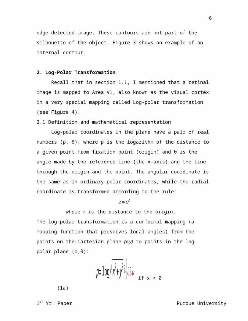
2.1 Definition and mathematical representation

Log-polar coordinates in the plane have a pair of real numbers (ρ, θ), where ρ is

the logarithm of the distance to a given point from fixation point (origin) and θ is the

angle made by the reference line (the x-axis) and the line through the origin and the point.

The angular coordinate is the same as in ordinary polar coordinates, while the radial

coordinate is transformed according to the rule:

r=eρ

where r is the distance to the origin.

The log-polar transformation is a conformal mapping (a mapping function that preserves

local angles) from the points on the Cartesian plane (x,y) to points in the log-polar plane

(ρ,θ):

ρ=log √x2+ y2¿ }¿¿¿ if x > 0 (1a)

ρ=log √x2+ y2¿ }¿¿¿if x < 0,

where signofy = the sign of y value (1b)

Figure 4 a) and b) shows how the mapping looks like on the Area V1 in the cortex. As we

can see Area V1 is not a plane. When the visual cortex is opened up, it looks like Figure

4 c).


5

Figure 4. After Schwartz (1980). a) Retina and b) the area V1 in the cortex

(Courtesy: http://fourier.eng.hmc.edu/e180/lectures/visualcortex/node8.html)

c) Idealized log-polar mapping.

(Courtesy: http://users.isr.ist.utl.pt/~alex/Projects/TemplateTracking/logpolar.htm)

The inverse transformation from Log-polar to Cartesian space is given by:

x=e ρ cosq ¿ }¿¿¿(2)

Figure 4a shows the retinal image mapped to the visual cortex and Figure 4b is the

geometric representation of log-polar mapping. A circle on the retina, whose center

coincides with the center of the retina, maps into straight line in the log-polar space.

Figure 5 shows hand-drawn examples in retinal/Cartesian space and their

mapping in log-polar space.


ρ

θ

http://users.isr.ist.utl.pt/~alex/Projects/TemplateTracking/logpolar.htm

http://fourier.eng.hmc.edu/e180/lectures/visualcortex/node8.html

6

Equation 1a and b are used to map the hand-drawn segments in Cartesian Space to

the Log-Polar Space. Equation 2 is used to map the hand-drawn segments in Log-Polar

Space to the Cartesian space. The green lines indicate axes with point (0, 0) being the

intersection of the green lines. This is the fixation point (center of the retina).

Cartesian Space Log-Polar Mapping

1.

2.

Figure 5. Examples of log-polar mapping. The ellipse in the log-polar window is used to visualize the ρ and

θ weights. These weights are explained in section 3.3 Modified Dijkstra.Variation in the weights reflects in

the size of the ellipse and is affected by both weight and range. If it is a circle, then in the graph, the

distance along ρ and θ are the real distance

2.2 Why Log-polar transformation?

After conducting experiments on several primates, Schwartz (1980) found that the

visual system does log-polar mapping of the retinal image to visual cortex. Since this


7

mapping happens naturally I used this transformation to see if relevant occluding and

internal contours could be retrieved.

As mentioned earlier, this transformation represents a circle in Cartesian space as

a straight line in log-polar space. As a result, a closed curve on the retina is often not far

from a straight line in V1.

We investigated computing the shortest path in log-polar space to identify closed

simple curves in the retinal image. We expect that finding/solving the shortest path

problem (not the algorithm) might be an intelligent interpolation technique capable of

making decision globally and producing closed simple curves. A path between a start and

end point such that the cost or distance of reaching the end point is minimum, is called a

shortest path (discussed in Section 3 in detail).

2.3 Why log to the base e?

The density of receptors on the retina is locally uniform but globally non uniform.

In area V1, the receptors are mapped, locally as well as globally, uniformly. For this to

happen the logarithmic base has to be “e”. Any other base will not give local as well as

global uniformity in area V1. Some of the properties of logarithmic conformal mapping

are that concentric circles (exponentially spaced) are mapped to vertical equidistant lines

and radial lines (with equal angular spacing) are mapped to horizontal equidistant lines

(Schwartz 1977).

3. Shortest Path

3.1 Theory of Shortest Path Problem

Before we talk about shortest path directly, it is useful to know about graph theory

briefly. In Computer science and Mathematics, a graph is defined as collection of vertices

or nodes and a collection of edges that connect pairs of vertices .The study of these

graphs is called graph theory. Traditionally an edge is allowed to connect to a node to

itself, but in this project for simplicity of computation we do not allow this, mainly

because it is redundant edge.

In graph theory, the shortest path problem is the problem of finding the shortest

distance between two vertices given connectivity information and edge weights, so that

the path obtained has the minimum of the sum of the constituent edges. Connectivity


8

information indicates whether an edge or connection exists between two nodes or vertices

and what the degree of each node/vertex is. The degree of a vertex is defined as the

number of edges incident with it. Here, the shortest path is computed for the undirected

graphs (explained later in this section). The Shortest path can be formally defined as

follows:

Given a weighted graph (that is, a set V of vertices, a set E of edges, and a real-valued

weight function f: E → R), and elements v and v' of V, find a path P (a sequence of

edges) from v to v' of V so that ∑p∈P

f ( p)is minimal among all paths connecting v to v’

(Cormen et al., 2011c).

Formally a path is defined as follows:

A path of length k from a vertex u to a vertex u’ in a graph G = (V, E) is a sequence <

v0, v1, v2, . . ., vk > of vertices such that u = v0, u’ = vk, and (vi-1, vi )∈ E for i = 1, 2, … ,k, V =

vertices, and E = edges. The length of the path could be the number of edges or the

distance in the path. (Cormen et al., 2011d).

Figure 6. a) undirected graph b) fully connected undirected graph

There are two main kinds of graphs: Directed and undirected graphs. An

undirected graph is a graph where the edges between the nodes do not have direction

associated with them. In a fully connected graph, every node is connected to every other

node (Cormen et al., 2011b).


1

23

4 5

6

http://en.wikipedia.org/wiki/Real_number

9

Figure 6a shows an example of an undirected graph with circles representing

nodes and the integers within them representing their numbers and 6b shows an example

of a fully connected graph where each node is connected to every other node, where

vertices of the heptagon are the nodes.

There are various algorithms to compute the shortest path. For our purposes I use

the Dijkstra algorithm (explained in appendix).

Some of the properties of shortest path are:

1. Shortest paths are not necessarily unique.

2. Weights are not necessarily distances.

3. A shortest path between two vertices with one or more vertices between them

contains other shortest paths within it.

3.2 How does the Dijkstra algorithm work and why does it give the optimal shortest path

Consider a simple graph below with vertices/nodes A, B, C, D. The numbers

indicate the distances (costs).Note these costs are nonnegative as distance have to be

nonnegative values for this algorithm.

The output of Dijkstra would be the shortest distance between A and B, in this

case 6, which will include vertices(nodes) A, C, D and B as the shortest path( as indicated

by the arrows in the Figure7).

Figure 7. Simple graph that explains working of Dijkstra

The algorithm starts at vertex (node) A and sets the distance to itself initially,

which is zero. This is our base case or starting point. In other words, vertex (node) A is

the initial stating vertex (node) thus its zero. Then when the algorithm reaches any other

vertex the distance/weight get added to this value Next it checks the distance between

vertices (nodes) B and C, the next vertices (nodes) connected to A .However, note that

even if B vertex (node) is examined it is not marked visited. This vertex (node) gets the

distance value 10.The algorithm moves to the closest vertex (node) of the two (in this

example vertex (node) C) that keeps the total distance between A and next vertex


B 10<6

2 D

2

10A

2

C

10

(node) to a minimum, and adds the distance between A and C to the previous distance

(0+2=2). This process is repeated by moving to the next closest vertex till it reaches B

and examines all the possible paths to B. In the end, the previous distance value of B (For

example, path (AB) 10 > path (ACDB) 6,in this case. This just shows there are two paths

to get from A to B and we get two distances/weights d algorithm picks smallest of the

two values thus pick the path with smallest value) gets replaced by the new smaller value

found. It makes a local decision to choose a shortest path available even for a sub-

structure of the graph.

The final shortest path computed by Dijkstra is always the optimal path. Here is

an informal proof. We assume that the first choice made is a greedy choice to pick the

shortest path. The optimal solution to a sub-problem and greedy choice will give an

optimal solution to the problem. Thus Dijkstra always gives optimal shortest path. We

can use induction to formally prove it.

3.3 Modified Dijkstra

Since I want to apply shortest path in log-polar space, the original Dijkstra

algorithm needed to be modified such that the start and end point are the same point.

The graph created for this project is a fully connected undirected graph (explained

in section 3.1) thus a path always exists between any two nodes picked. This way we

don’t have the problem of unreachability. The weights/costs are the Euclidean distance

values computed (see equations below).

For hand drawn images (Figure 5), the pixels selected by the mouse are

automatically stored as points thus edge detection is not needed. Here by “edge” we mean

a geometric line for a figure. For example, in Figure 5 images would be the white pixels

grouped together and for each such edge the start point and end point are the only nodes

used for the graph. This edge we call it existing edge which is visible. In a graph structure

it is a connection between two nodes. For the purpose of this paper when we talk of a

point it mean a pixel and vise versa, and these points are the nodes in a graph structure.

For real images, we begin with canny edge detection (one of the most common edge

detection algorithms). A white pixel on the edge is a node of a fully connected graph

(explained in section 3.1). The edges are invisible in the images and are internal to the

program .They are in the form of matrix representing the connectivity. This is done for


11

computational convenience. The scene in the image is now represented in the form of a

graph structure. The distance is computed for the start and end point of an existing edge

to every node.

The cost function formulae in the log-polar space are given as follows:

Let p be point 1 with coordinates (θ1, ρ1). Let q be point 2 with coordinates (θ2,

ρ2).Let d be the Euclidean distance between p and q given by the formula:

d=√(θ1−θ2 )2∗wx2+wy2 ( ρ1−ρ2)2

Where wx and wy are the weights along the axes. In the current implementation,

these weights are set to 1.

On-curve or existing edge cost function: αd

Off-curve or interpolated edge cost function:

e(βd−1)

whereα=0.5 and β=1 are the multiplying factors, and d is the weighted Euclidean

distance.

Recall from section 2.1 that the coordinates of log-polar space are ρ and θ. Thus the cost

functions would be computed according to the new coordinate system where points p and

q would be represented in terms of ρ and θ.

The fixation point must be inside the region representing the object. The start-end

point is selected manually. Alternatively, a number of starting points can be tried.

3.4 Runtime complexity

The Dijkstra is a polynomial time algorithm. It has a run time of O(nlogn).

4. The Computation and Results

4.1Method

I pick a start point in log-polar space such that the fixation point, indicated by the

intersection of the axes (green lines) in Cartesian space, is within the object. This start

point corresponds to a node in the graph e.g a point on the existing edge . The shortest

path is computed from this point to itself when there is no edge drown from this point to

itself, in log-polar space using Dijkstra’s algorithm, discussed earlier, and the output

shown by pink curve is mapped back to the Cartesian space using Equation 2 (see Figure

8 for output).The pink curve represents the path that generated the shortest distance using


12

the algorithm. Note that in logpolar space the circle is a straight line thus a single point on

circle will be represented as start and end point in logpolar space. Thus in logpolar space

even if we pick only one point it is internally the start and the end point between which

we compute the shortest path.


13

Figure 8. Examples showing the shortest Paths in log-polar representation

Recall that an occluding contour is a closed non-self-intersecting curve. The

shortest path in the log-polar representation (area V1) corresponds to a maximally


Cartesian space Log-Polar

Mapping

Shortest Path

output in

Cartesian

space

Shortest path

in Log-polar

space

1.

2.

3.

4.

5.

14

circular, closed curve in the retinal image. Example 3 shows that shortest path (outcome

path) makes a decision about when an edge common to two objects would be considered

part of which object depending on where the fixation point is located (The decision

making has been discussed in details in later section). Recall that the fixation point is the

origin and the control panel has the option to select to move the fixation point around by

the user. The graph and the distances computed are updated automatically with reference

to the fixation point. Example 5 demonstrates that the shortest path is capable of

eliminating the noise and keeping the edges important to the object.

4.2 Local interpolation versus Global interpolation

Before we get into local and global interpolation it is necessary to understand

what it means by interpolation and what kinds of interpolation techniques exist.

Interpolation means estimating the data points based on some pre-existing data sets.

There are various interpolation techniques like piecewise interpolation, linear

interpolation etc. based on the mathematical function used. These techniques are

classified based on what the final outcome is, for example local and global interpolation.

Local interpolation means that the interpolation techniques lead to the decision of

which path to continue on based on the local information. The local interpolators apply

an algorithm repeatedly to a small portion of the total set of points. For example, Figure

9a shows one of the paths that could be taken. The decision here would depend on the

immediate connecting contours or the contours in the local region. An example of local

interpolation is piecewise linear interpolation.

Global interpolation means the decision about which path to continue on depends

on the information obtained from the entire image. For example, Figure 9b illustrates that

moving one of the edges changes the decision at the intersection. Thus, a change far away

in the image affects the decision at the highlighted intersection. An example of global

interpolation is shortest path.


15

Figure 9a) Local co-linearity of edges is ignored. The blue dashed circle indicates the region of decision

making.

9b) Interpretation of a junction can change by a spatially remote feature – see Figure 8 for more examples.

Red segment marked is the selected segment to move in the scene. The blue dashed circle indicates the

region of decision making.

The examples above illustrate that shortest path is spatially global in the sense

that a change far away in the image affects the path taken. An advantage of having global

interpolators is that they tend to produce smoother contours with less abrupt changes.


16

5. Advantages of running the shortest path in Log-polar representation

5.1 Closure

Running the shortest path in log-polar space leads to a closed curve. So, this is

like solving a Traveling Salesman Problem using a fast algorithm and ignoring contours

that are likely to be irrelevant.

5.2 Real Images (high resolution –low resolution)

Coming back to the original problem of analyzing real images and contour

analyses we apply the shortest path in log-polar space after doing canny edge detection

on the gray scale images. The Bumblebee camera images used had a resolution of

800x600.The cannon camera was used to get high resolution images (4752x3168).

Gray Scale

Image

Edge detection (input) Shortest Path (output)

Cartesian

Space

Log-polar

Space

Cartesian

Space

Log-Polar

Space

a)

b)

c)

Figure 10 Note: As the fixation point changes the log-polar mapping also changes accordingly. a) A real image with extracted occluding contour of a small chair

b) Large chairc) Rocking horse


17

The low resolution images as shown in Figure 10 gave good occluding contour for

different objects in the same scene when we picked a fixation point within each object

and one start point on the object contour. This is however assuming that we know where

the objects are in a given scene. Figure 11 on next page shows more examples of

occluding contours obtained for various objects in real images obtained by α=0.5 ,

β=1.

Edge detected image with shortest path output

Gray Scale image Log-polar image with shortest path output

1

2


18

3

4

5

Figure 11 Examples of occluding contour for various objects in real images obtained by ¿0.5 ,β=1.


19

Randomly choosing multiple start points for each object and running the shortest

path in log-polar space gave most of the relevant contours of the object (see Figure12).

Figure 12 Output for one object after background has been removed.

Figure13 is an example of high resolution image after edge detection. It is not

clear, at this point, how much benefit there is when high resolution images are used.


20

Figure 13.a) Part of High resolution Cannon image of Book shelf (in Cartesian space)

b)Part of High resolution Cannon image of Book shelf(in Cartesian space) with occluding contour obtained

by computing shortest path(pink color) in log-polar space with α=0.5 ,β=1

6. Summary

In summary, i) log-polar space produces simple closed curves which represent

occluding contours, and ii) having a fixation point inside the object and computing

shortest path automatically eliminates a lot of noise keeping only relevant contours useful

to represent the object.

7. Appendix

Dijkstra’s algorithm

Dijkstra’s algorithm is a graph search algorithm that is commonly used to solve a

shortest path problem for a graph with nonnegative costs for edges. As mentioned earlier

the cost values don’t necessarily have to be distances. The basic idea of this algorithm is

as follows:

1. Mark all the nodes of the graph as unvisited.


1

52

3 4

6

21

2. Assign tentative distance to all other nodes. For example for the start node set

the value to be zero and infinity for all other nodes.

3. At each iteration, select a current node. For the first node the distance will be 0,

since it is the starting node. But for next iterations the current node will be the closest

unvisited node to the starting node. In case of a tie the first found node will be picked.

4. For the current node, compute the tentative distances to its connecting nodes

from starting node. For example, in Figure 7, if the current node is C and its tentative

distance s marked as 2 ,and the connecting edge D has a length 2,then the distance to D

will be 2+2 = 4.If this distance is less than the previous recoded distance for D, then

replace it with the new distance found.

5. A node is marked a visited only after all its connecting nodes are examined. By

“examined” means whether to mark it as the node to move or not based on the final cost

to reach the final destination node . The next closest node with lowest tentative distance

will now be the current node and we repeated this process till we reach the destination

(Cormen et al., 2001a).

The graph is in the form of an adjacency matrix usually, where the adjacency

matrix provides information about which vertices are adjacent to one another. If there

exists an edge between two vertices, this is represented by a 1. If there is no edge

between two vertices, this is represented by a 0. For example, Figure 14a is a labeled

graph and its adjacency matrix is shown in Figure 14b (Cormen et al., 2001b).

(1 1 0 0 1 01 0 1 0 0 00 1 0 1 0 10 0 1 0 1 11 0 0 1 0 00 0 1 1 0 0

)


22

Figure 14.a).Labeled Graph b) adjacency matrix

The advantage of using an adjacency matrix is that it is symmetrical. Therefore,

when dealing with huge images or high-resolution images I can use only the upper

triangular matrix, thus saving memory, and take the mirror symmetric matrix for

computation.

8. Acknowledgement This research was supported by the NSF. The author is grateful to

Dr. Li for providing computer algorithms.

9. References:

1.Cormen, T. H.; Leiserson, C. E.; Rivest, R. L.; Stein, C. (2001a) "Section 24.3:

Dijkstra's algorithm". Introduction to Algorithms (2nd ed.). MIT Press and McGraw-Hill.

pp. 595–601.

2. Cormen, T. H.; Leiserson, C. E.; Rivest, R. L.; Stein, C. (2001b) "Section 22.1:

Representations of graphs". Introduction to Algorithms (2nd ed.). MIT Press and

McGraw-Hill. pp. 527–531.

3. Cormen, T. H.; Leiserson, C. E., Rivest, R. L., Stein, C. (2001c) "Single-Source

Shortest Paths and All-Pairs Shortest Paths". Introduction to Algorithms (2nd ed.). MIT

Press and McGraw-Hill. pp. 580–642.

4. Cormen, T. H.; Leiserson, C. E., Rivest, R. L., Stein, C. (2001d) "B.4 Graphs".

Introduction to Algorithms (2nd ed.). MIT Press and McGraw-Hill. pp. 1080–1081

5. Lim F. L., West G.A.W., Venkatesh S. (1997) Use of log polar space for foveation

and feature recognition IEE Proc -Vis Image Signal Process, 144, 323-331.

6. Malik, J., Belongie, S., Leung, T. And Shi, J. (2001) Contour and Texture Analysis for

Image Segmentation. International Journal of Computer Vision 43(1), 7–27.

7. Marr, D. (1982) Vision. W.H. Freeman and Company.


23

8. Klinkenberg, .B (1997). UNIT 40 - SPATIAL INTERPOLATION I.

http://www.geog.ubc.ca/courses/klink/gis.notes/ncgia/u40.html# SEC40.2.2

9. Schwartz, E.L. (1980) Computational anatomy and functional architecture of striate

cortex: A spatial approach to perceptual coding. Vision Research, 20, 645-669.

10. Schwartz, E.L. (1977) Spatial mapping in the Primate Sensory Projection: Analytic

Structure and Relevance to Perception. Biological Cybernetics, 25, 181-194.

11. Wertheimer, M. 1938. Laws of organization in perceptual forms (partial translation).

W. Ellis (Ed.). In A Sourcebook of Gestalt Psychology. Harcourt Brace and

Company, pp. 71–8


gupte - first year paper_approved (1)

Documents

irrelevant contours

meaningful contours

internal contours

real contours

occluding contours

d representation

d images

human visual system