guideline on the meaning and the use of precision and bias...

Guideline on the Meaning and the Use Of Precision and Bias Data Required by 40 CFR Part 58 Appendix A

Version 1.1

EPA-454/B-07-001

October, 2007

Guideline on the Meaning and the Use of Precision and Bias Data Required by 40 CFR Part 58 Appendix A

By: Louise Camalier

Shelly Eberly Jonathan Miller Michael Papp

Version 1.1

U.S. Environmental Protection Agency

Office of Air Quality Planning and Standards Air Quality Assessment Division

Air Quality Analysis Group Research Triangle Park, North Carolina

ii

Foreword

The EPA’s Ambient Air Quality Monitoring Program is implemented under the authority of the Clean Air Act to provide air quality data:

1. Provide air pollution data to the general public in a timely manner. 2. Support compliance with air quality standards and emissions strategy development 3. Support air pollution research studies.

EPA recognizes the importance of collecting data across the nation that one can be assured that it was of acceptable and consistent quality. The ambient air monitoring regulations were revised in 1979 and at that time two Appendices were added: • Appendix A- Quality Assurance Requirements for State and Local Monitoring Stations • Appendix B-Quality Assurance Requirements for Prevention of Significant Deterioration

Monitoring A 1983 guidance document titled “Guideline on the Meaning and Use of Precision and Accuracy Data Required by 40 CFR Part 58 Appendices A and B was developed as a companion document to the Appendices to help explain the rational for the statistics and their use. On October 17, 2006 the EPA Administrator signed the Ambient Air Monitoring Rule. This rule changed a number of requirements in 40 CFR Appendix A. One important change was the statistical techniques use estimate the precision and bias of the various quality control and performance evaluation checks included in Appendix A. The objective of this Guideline is to provide the monitoring organization with a description of the ambient air monitoring quality system, the quality control techniques in the Appendix A regulations and provide the guidance and spreadsheets necessary for to understand and implement these statistics. This document is intended to the replace the 1983 Guideline. The document is separated into two sections. Section 1 provides the background and rationale for the statistics while Section 2 provides the guidance for the new statistics. Those just interested in how to calculate the new statistics may want to proceed to Section 2. The statements in this document, with the exception of referenced requirements, are intended solely as guidance. This document is not intended, nor can it be relied upon, to create any rights enforceable by any party in litigation with the United States. EPA may decide to follow the guidance provided in this document, or to act at variance with the guidance based on its analysis of the specific facts presented. This guidance may be revised without public notice to reflect changes in EPA’s approach to implementing 40 CFR Part 58, Appendix A. This document is available on hardcopy as well as accessible as a PDF file on the Internet under the Ambient Monitoring Technical Information Center (AMTIC) Homepage (http://www.epa.gov/ttn/amtic/pmqa.html). The document can be read and printed using Adobe Acrobat Reader software, which is freeware that is available from many Internet sites (including the EPA web site).

iii

Table of Contents Section Page Foreward ........................................................................................................................................ iii Table of Contents........................................................................................................................... iv List of Figures ................................................................................................................................ iv List of Tables ...................................................................................................................................v List of Acronyms .............................................................................................................................v 1.0 Introduction...............................................................................................................................1

1.1 Goal of the Guideline...............................................................................................1 1.2 Background .............................................................................................................1 1998-2000 PM2.5 and the National Ambient Air Monitoring Strategy ...............2 1.3 Link between Data Quality Objectives, Data Quality Indicators and Measurement Quality Objectives.............................................................................3 Data Quality Objectives........................................................................................3 Data Quality Indicators .........................................................................................4 Measurement Quality Objectives..........................................................................5 Measurement Quality Data Aggregation-The Primary Quality Assurance Organization..........................................................................................................6 1.4 The Development of the New Statistics...................................................................8

2.0 The New Statistics: A Fool-Proof Method and DASC Tool ..................................................12

2.1 Gaseous Precision and Bias Assessment ...............................................................14 2.2 Precision Estimates from Collocated Samples ......................................................17 2.3 PM2.5 Bias Assessment ..........................................................................................19 2.4 PM2.5, PM10-2.5 Absolutes Bias Assessment.......................................................... 21 2.5 One-Point Flow Rate Bias Assessment..................................................................23 2.6 Semi- Annual Flow Rate Audits ............................................................................25

List of Figures

Figure Page 1 Effect of positive bias on the annual average estimate resulting in an incorrect

declaration on non-attainment..............................................................................................3 2 Effect of negative bias on the annual average estimate resulting in an incorrect

declaration on attainment.....................................................................................................3 3 Relationship of data quality objectives to data quality indicators, measurement

quality objectives and data quality assessments ..................................................................4 4 Precision and bias estimates for a hypothetical example.....................................................9 5 DASC Main Menu .............................................................................................................12 6 Gaseous Precision and Bias DASC Worksheet ................................................................14 7 Collocated Precision DASC Worksheet ...........................................................................17 8 PM2.5 Bias DASC Worksheet...........................................................................................19 9 Absolute Bias DASC Worksheet ......................................................................................21 10 One-Point Flow Rate DASC Worksheet ...........................................................................23 11 Semi-Annual Flow Rate Audits DASC Worksheet ...........................................................25 12 Lead Bias DASC Worksheet .............................................................................................27

iv

List of Tables Table Page 1 Ambient Air Monitoring Measurement Quality Samples....................................................6 2 Reporting Organization (Old) and Primary Quality Assurance Organization (New)

Definitions in 40 CFR Part 58 Appendix A.........................................................................7 3 Data Quality Indicators Calculated for Each Criteria Pollutant.........................................12 4 Minimum Concentration Levels for Particulate Matter Precision Assessments. ..............17

Acronyms AQS Air Quality System AMTIC Ambient Monitoring Technology Information Center CASAC Clean Air Scientific Advisory Committee CFR Code of Federal Regulations CV coefficient of variation DASC data Assessment Statistical Calculator DQA data quality assessment DQI data quality indicator DQO data quality objective EDO environmental data operation EPA U.S. Environmental Protection Agency FW focus workgroup MQO measurement quality objective NAAQS National Ambient Air Quality Standards NPAP National Performance Audit Program OAQPS Office of Air Quality Planning and Standards ORD Office of Research and Development P&A precision and accuracy PEP Performance Evaluation Program PM2.5 particulate matter < 2.5 microns PQAO primary quality assurance organization QA/QC quality assurance/quality control QA quality assurance QAPP quality assurance project plan SLAMS state and local monitoring stations SOPs standard operating procedures

v

P&B Guidance Version 1.1

October 2007

Section 1: Introduction 1.1 Goal Of the Guideline On October 17, 2006 the EPA amended its national air quality monitoring requirements. This rule changed a number of requirements in 40 CFR Part 58 Appendix A, the section which describes the planning, implementation, assessment and reporting of the ambient air monitoring quality system. One important change was the statistical techniques used to estimate the precision and bias of the various quality control and performance evaluation checks included in Appendix A. Prior to this revision, the statistics used to estimate precision and bias (then called accuracy) where developed in the late 1970’s. In 1983, the guidance document titled “Guideline on the Meaning and Use of Precision and Accuracy Data Required by 40 CFR Part 58 Appendices A and B”1 (hereafter referred to as “1983 Guideline”) was developed as a companion to Appendix A and B to help explain the rationale for the statistics and how they were used. The objective of this new Guideline is to provide the data user with a brief history of the establishment of the ambient air monitoring quality system, the quality control techniques that have been in place up until the promulgation of the new monitoring rule, and to provide the guidance and spreadsheets necessary to understand and implement these new statistics. This document is intended to the replace the 1983 Guideline. 1.2 Background The EPA’s Ambient Air Quality Monitoring Program is implemented under the authority of the Clean Air Act to provide air quality data for one or more of the three following objectives:

• Provide air pollution data to the general public in a timely manner. • Support compliance with air quality standards and emissions strategy development. • Support air pollution research studies.

In order to support the objectives the monitoring networks are designed with a variety of monitoring sites that generally fall into the following categories which are used to:

1. determine the highest concentrations expected to occur in the area covered by the network;

2. determine typical concentrations in areas of high population density; 3. determine the impact on ambient pollution levels of significant sources or source

categories; 4. determine the general background concentration levels; 5. determine the extent of regional pollutant transport among populated areas, and in

support of secondary standards; and

1 http://www.epa.gov/ttn/amtic/cpreldoc.html

1


October 2007

6. measure air pollution impacts on visibility, vegetation damage, or other welfare- based impacts.

These different objectives can potentially require information of varying quality. EPA recognized the importance of collecting data of acceptable and consistent quality. In the late 1970’s EPA started developing consistent techniques to identify the objectives that required the highest quality data and then to develop a set of requirements to collect and assess this measurement quality information. The EPA embarked on the process very similar to what is now called the Data Quality Objectives (DQO) Process and determined that the comparison of data to the National Ambient Air Quality Standards (NAAQS) was the highest priority objective and that data would be collected in a manner that minimized the uncertainty in making attainment decisions. The ambient air monitoring regulations were revised in 1979 and at that time two Appendices were added:

• Appendix A- Quality Assurance Requirements for State and Local Monitoring Stations (SLAMS)

• Appendix B-Quality Assurance Requirements for Prevention of Significant Deterioration (PSD) Monitoring

These appendices established the development of a quality assurance program to be implemented at the reporting organization level of aggregation. The appendices identified quality control, audits and performance evaluation techniques that would be implemented internally as well as by external organizations like the EPA Regions, ORD and OAQPS, and established the statistical techniques to evaluate the data quality indicators. The primary data quality indicators for the ambient air program were identified as precision and accuracy (P&A). The 1983 Guideline provided a rationale for the use of the P&A data that was required to be collected in the two appendices mentioned. As was written in the 1983 Guideline, “the P&A statistics represented a compromise between (a) theoretical statistical exactness, and (b) simplicity and uniformity in computational procedures”. The P&A statistics were aggregated by reporting organization over various time periods and combined into a probability limit estimate. 1998-2000 PM2.5 and the National Ambient Air Monitoring Strategy In 1998, with the promulgation of the PM2.5 NAAQS, EPA formally implemented the DQO process and established acceptance criteria for precision and bias using statistics which were a departure from the statistics in the 1983 Guideline. During this time period, OAQPS and the monitoring organizations were cooperating to develop a new Monitoring Strategy2. OAQPS formed a QA Strategy Workgroup that set out to perform a thorough review of the Appendix A requirements and improve the quality system where appropriate. One outcome of this review was the suggestion that EPA look at a way to provide a more consistent set of statistics for the estimates of precision and bias. As part of this process, the Workgroup endorsed the use of the DQO process and the measurement quality objectives (MQOs) that lead to attainment of the DQOs.

2 DRAFT National Ambient Air Monitory Strategy, December 2005 http://www.epa.gov/ttn/amtic/monstratdoc.html

2


October 2007

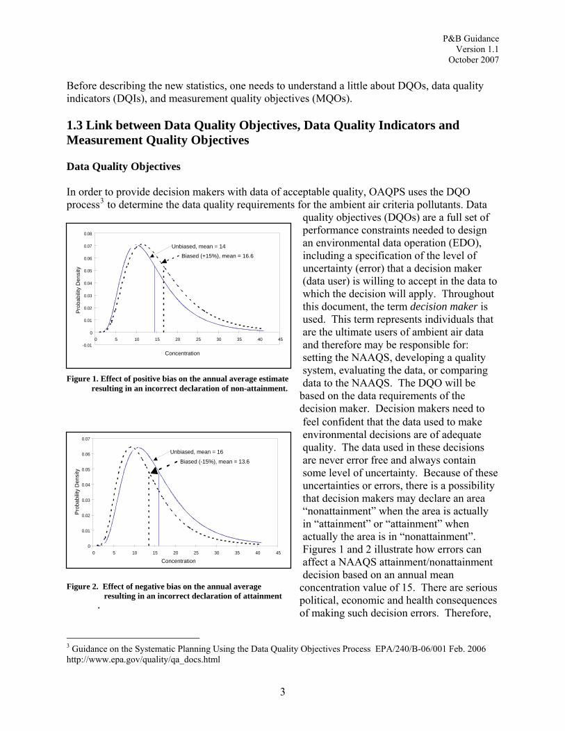
Before describing the new statistics, one needs to understand a little about DQOs, data quality indicators (DQIs), and measurement quality objectives (MQOs). 1.3 Link between Data Quality Objectives, Data Quality Indicators and Measurement Quality Objectives Data Quality Objectives In order to provide decision makers with data of acceptable quality, OAQPS uses the DQO process3 to determine the data quality requirements for the ambient air criteria pollutants. Data

quality objectives (DQOs) are a full set of performance constraints needed to design an environmental data operation (EDO), including a specification of the level of uncertainty (error) that a decision maker (data user) is willing to accept in the data to which the decision will apply. Throughout this document, the term decision maker is used. This term represents individuals that are the ultimate users of ambient air data and therefore may be responsible for: setting the NAAQS, developing a quality system, evaluating the data, or comparing data to the NAAQS. The DQO will be

based on the data requirements of the decision maker. Decision makers need to feel confident that the data used to make environmental decisions are of adequate quality. The data used in these decisions are never error free and always contain some level of uncertainty. Because of these uncertainties or errors, there is a possibility that decision makers may declare an area “nonattainment” when the area is actually in “attainment” or “attainment” when actually the area is in “nonattainment”. Figures 1 and 2 illustrate how errors can affect a NAAQS attainment/nonattainment decision based on an annual mean

concentration value of 15. There are serious political, economic and health consequences of making such decision errors. Therefore,

-0.01

0

0.01

0.02

0.03

0.04

0.05

0.06

0.07

0.08

0 5 10 15 20 25 30 35 40 45

Concentration

Pro

babi

lity

Den

sity

Unbiased, mean = 14 Biased (+15%), mean = 16.6

Figure 1. Effect of positive bias on the annual average estimate resulting in an incorrect declaration of non-attainment.

0

0.01

0.02

0.03

0.04

0.05

0.06

0.07

0 5 10 15 20 25 30 35 40 45

Concentration

Prob

abilit

y D

ensi

ty

Unbiased, mean = 16 Biased (-15%), mean = 13.6

Figure 2. Effect of negative bias on the annual average resulting in an incorrect declaration of attainment

.

3 Guidance on the Systematic Planning Using the Data Quality Objectives Process EPA/240/B-06/001 Feb. 2006 http://www.epa.gov/quality/qa_docs.html

3


October 2007 decision makers need to understand and set limits on the probabilities of making incorrect decisions with these data. In order to set probability limits on decision errors, one needs to understand and attempt to control uncertainty. Uncertainty is used as a generic term to describe the sum of all sources of error associated with an EDO. Uncertainty can be illustrated as follows:

222mpo SSS +=

where: So= overall uncertainty Sp= population uncertainty (spatial and temporal) Sm= measurement uncertainty (data collection).

Figure 3 provides a description of the relationship between uncertainty and the DQO. The estimate of overall uncertainty is an important component in the DQO process. Both population and measurement uncertainties must be understood. The DQOs are assessed through the use of data quality indicators (DQIs) which are the quantitative statistics and the qualitative descriptors used to interpret the degree of acceptability or utility of data to the user. The DQIs can then be used to establish the MQOs which will be discussed below. Once the MQOs are

established and monitoring is implemented, data quality assessments (DQAs) are performed to determine whether the DQOs were achieved. If not, the monitoring program should take steps to identify the major sources of uncertainty and find ways to reduce these uncertainties to the acceptable levels.

Uncertainty = Population + Measurement

2.Precision3.Bias4. Completeness5. Comparability6. Detectability

MQOs

PreparationField

Laboratory

DQO

DQA

}1. Representativeness

Data Quality IndicatorsUncertainty = Population + Measurement

2.Precision3.Bias4. Completeness5. Comparability6. Detectability

MQOs

PreparationField

Laboratory

DQO

DQA

}1. Representativeness

Data Quality Indicators

Figure 3. Relationship of data quality objectives to data quality indicators, measurement quality objectives and data quality assessments.

Data Quality Indicators The data quality indicators are:

Representativeness - the degree in which data accurately and precisely represents a characteristic of a population, parameter variation at a sampling point, a process condition, or an environmental condition. Precision - a measure of mutual agreement among individual measurements of the same property usually under prescribed similar conditions. This is the random component of error. Precision is estimated by various statistical techniques using some derivation of the standard deviation.

4


October 2007 Bias - the systematic or persistent distortion of a measurement process which causes error in one direction. Bias will be determined by estimating the positive and negative deviation from the true value as a percentage of the true value. Detectability - the determination of the low range critical value of a characteristic that a method specific procedure can reliably discern. Completeness- a measure of the amount of valid data obtained from a measurement system compared to the amount that was expected to be obtained under correct, normal conditions. Comparability - a measure of confidence with which one data set can be compared to another

Accuracy has been a term frequently used to represent closeness to “truth” and includes a combination of precision and bias error components. This term had been used throughout the CFR but has been replaced with bias when there is the ability to distinguish precision from bias. The quality system for the ambient air monitoring program focuses on understanding and controlling (as much as possible) measurement uncertainty and because of that, mainly focuses on the data quality indicators of precision, bias, detectability completeness and comparability. Representativeness is addressed through network designs and is not, per-se, something that the quality system can control through better measurements. Measurement Quality Objectives For each DQI one must identify a level of uncertainty or error that is acceptable and will achieve the DQO. MQOs are designed to evaluate and control various phases (sampling, preparation, analysis) of the measurement process to ensure that total measurement uncertainty is within the range prescribed by the DQOs. This finally gets us to CFR where the various quality control checks, like the one point quality control check for the gaseous pollutants or the particulate matter collocated instruments, are established. These checks help quantify a data quality indicator and their acceptance criteria are the MQOs. Table 1 provides a complete listing of the required measurement quality checks and the MQOs as they are currently defined in Appendix A. EPA has not changed the types of samples it uses to assess precision and bias. Although the 2006 rule has changed some of the names and some of their sampling frequencies, the basic checks are the same. Although the types of checks have not changed, EPA changed the statistics used to evaluate precision and bias and in some cases how the measurement quality data are aggregated.

5


October 2007

Table 1. Ambient Air Monitoring Measurement Quality Samples (Table A-2 in 40 CFR Appendix A)

Method CFR Reference Coverage (annual) Minimum frequency MQOs*

Automated Methods

One-Point QC: for SO2, NO2, O3, CO

Section 3.2.1

Each analyzer

Once per 2 weeks

O3 Precision 7%, Bias + 7%. SO2, NO2, CO Precision 10% , Bias + 10%

Annual performance evaluation

for SO2, NO2, O3, CO

Section 3.2.2

Each analyzer

Once per year

< 15 % for each audit concentration

Flow rate verification PM10,PM2.5, PM10-2.5

Section 3.2.3 Each sampler Once every month < 4% of standard and 5% of design value

Semi-annual flow rate audit PM10, PM2.5, PM10-2.5

Section 3.2.4 Each sampler Once every 6 months

< 4% of standard and 5% of design value

Collocated sampling PM2.5, PM10-2.5

Section 3.2.5 15% Every twelve days

PM2.5, - 10% precision PM10-2.5- - 15% precision

PM Performance evaluation program PM2.5,PM10-2.5

Section 3.2.7 1. 5 valid audits for primary QA orgs, with < 5 sites 2. 8 valid audits for primary QA orgs, with > 5 sites 3. All samplers in 6 years

over all 4 quarters

PM2.5, - + 10% bias PM10-2.5- - +15% bias

Manual Methods

Collocated sampling PM10, TSP, PM10-2.5, PM2.5

3.3.1 and 3.3.5 15% Every 12 days PSD -every 6 days

PM10, TSP, PM2.5, - 10% precision PM10-2.5- - 15% precision

Flow rate verification PM10 (low Vol),PM10-2.5, PM2.5

3.3.2 Each sampler Once every month


Flow rate verification PM10 (High-Vol), TSP

3.3.2 Each sampler Once every quarter < 10% of standard and design value

Semi-annual flow rate audit PM10 (low Vol), PM10-2.5, PM2.5

3.3.3 Each sampler, all locations

Once every 6 months


Semi-annual flow rate audit PM10 (High-Vol), TSP

3.3.3

Each sampler, all locations

Once every 6 months

< 10% of standard and design value

Manual Methods Lead

3.3.4 1. Each sampler

2. Analytical (lead strips)

1. Include with TSP 2. Each quarter

1. Same as for TSP. 2. - + 10% bias

Performance evaluation program PM2.5, PM10-2.5

3.3.7 and 3.3.8 1. 5 valid audits for primary QA orgs, with < 5 sites 2. 8 valid audits for primary QA orgs, with > 5 sites 3. All samplers in 6 years

Over all 4 quarters PM2.5, + 10% bias PM10-2.5-, +15% bias

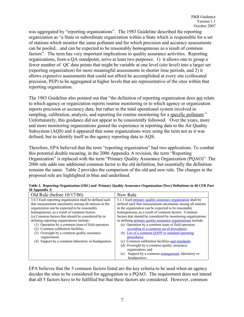
* Some of the MQOs are found in CFR and others in the QA Handbook Vol II (Appendix 15) which is under revision during the development of this guidance document. Measurement Quality Data Aggregation –The Primary Quality Assurance Organization In order to assess whether or not measurement quality data meet the established DQOs, the data must be aggregated in an appropriate manner. Prior to the new rule, measurement quality data

6


October 2007 was aggregated by “reporting organizations”. The 1983 Guideline described the reporting organization as “a State or subordinate organization within a State which is responsible for a set of stations which monitor the same pollutant and for which precision and accuracy assessments can be pooled…and can be expected to be reasonably homogeneous as a result of common factors”. The term has very important implications to quality assurance activities. Reporting organizations, from a QA standpoint, serve at least two purposes: 1) it allows one to group a fewer number of QC data points that might be variable at one level (site level) into a larger set (reporting organization) for more meaningful assessments in shorter time periods, and 2) it allows expensive assessments that could not afford be accomplished at every site (collocated precision, PEP) to be aggregated at higher levels that are representative of the sites within that reporting organization. The 1983 Guideline also pointed out that “the definition of reporting organization does not relate to which agency or organization reports routine monitoring or to which agency or organization reports precision or accuracy data, but rather to the total operational system involved in sampling, calibration, analysis, and reporting for routine monitoring for a specific pollutant.” Unfortunately, this guidance did not appear to be consistently followed. Over the years, more and more monitoring organizations gained the experience in reporting data to the Air Quality Subsystem (AQS) and it appeared that some organizations were using the term not as it was defined, but to identify itself as the agency reporting data to AQS. Therefore, EPA believed that the term “reporting organization” had two applications. To combat this potential double meaning, in the 2006 Appendix A revision, the term “Reporting Organization” is replaced with the term “Primary Quality Assurance Organization (PQAO)”. The 2006 rule adds one additional common factor to the old definition, but essentially the definition remains the same. Table 2 provides the comparison of the old and new rule. The changes in the proposed rule are highlighted in blue and underlined. Table 2. Reporting Organization (Old ) and Primary Quality Assurance Organization (New) Definitions in 40 CFR Part 58 Appendix A Old Rule (before 10/17/06) New Rule 3.0.3 Each reporting organization shall be defined such that measurement uncertainty among all stations in the organization can be expected to be reasonably homogeneous, as a result of common factors. (a) Common factors that should be considered by in defining reporting organizations include: (1) Operation by a common team of field operators (2) Common calibration facilities. (3) Oversight by a common quality assurance organization. (4) Support by a common laboratory or headquarters.

3.1.1 Each primary quality assurance organization shall be defined such that measurement uncertainty among all stations in the organization can be expected to be reasonably homogeneous, as a result of common factors. Common factors that should be considered by monitoring organizations in defining primary quality assurance organizations include: (a) Operation by a common team of field operators according to a common set of procedures; (b) Use of a common QAPP or standard operating procedures; (c) Common calibration facilities and standards; (d) Oversight by a common quality assurance organization; and

(e) Support by a common management, laboratory or headquarters.

EPA believes that the 5 common factors listed are the key criteria to be used when an agency decides the sites to be considered for aggregation to a PQAO. The requirement does not intend that all 5 factors have to be fulfilled but that these factors are considered. However, common

7


October 2007 procedures and a common QAPP should be strongly considered as key to making decisions to consolidate monitoring sites into a PQAO. Some of the precision and bias statistics can be evaluated at the site or instrument level; others must be evaluated at the PQAO level. In general, any measurement quality sample in Table 1 that has a coverage indicated as “each sampler/analyzer” can and will be evaluated at the site/instrument level. This data can also be aggregated at the PQAO level and the precision and bias statistics perform the appropriate evaluation at both site and PQAO level. Because only a percentage of sites in any monitoring organization implement collocated sampling and the Performance Evaluation Program (PEP) in any one year, the data must be aggregated and evaluated at the PQAO level. Although this particulate matter measurement quality data should be used to evaluate the instruments from which the checks are made, the data aggregation to the PQAO to assess the achievement of the DQO is of primary importance. 1.4 The Development of the New Statistics As mentioned earlier in this document, a Focus Workgroup (FW), a subset of the QA Strategy Workgroup, was formed to review and revise the precision and bias statistics. The FW proposed that the MQOs be based on confidence intervals. That is, determining whether the bias and precision variables meet the measurement quality objectives will be based on whether the confidence intervals for these variables meet the measurement quality objectives. The intent of this is two-fold. One reason for using confidence intervals is to be confident the measurement quality objectives are being met. It is different to say the bias is 5% plus or minus 10% compared to saying the bias is 5% plus or minus 1%. A second, and very practical, reason for using confidence intervals is to allow organizations that show tight acceptable results the flexibility in reducing the frequency of certain QC checks. For example, the site with a bias of 5% plus or minus 1% likely does not need as many QC checks as the site with the bias of 5% plus or minus 10%. The acceptance criteria are based on the number of years of data that coincide with the time frame of the ambient air quality standards. For example, since the 8-hour ozone standard is based on 3 years of data, the acceptance criteria for bias and precision will also be based on 3 years of data. Additionally, the acceptance criteria apply to each site operating an automated method. For the automated methods, estimates of both bias and precision are derived from the one-point quality control checks and then double-checked with the annual performance evaluations, independent State audits and the NPAP Program. To test the reasonableness of estimating bias and precision from bi-weekly checks, the FW made up some actual/indicated pairs, assuming different levels of bias and precision, and tested a couple of proposed statistics. The FW simulated 3 years of data and provided summary statistics at the quarterly, annual, and 3-year level. For each scenario, the data was summarized by the three methods below

1. CFR Probability Interval. For these statistics, EPA reviewed what was currently in CFR, namely the overall percent difference in the actual and indicated concentrations and an associated probability interval that shows where 95% of all the percent differences should fall. Note that this does not provide separate estimates of bias and precision.

8


October 2007 2. Signed Bias & Precision (CV). For this case, EPA estimate bias and precision

separately and also estimated confidence intervals for bias and confidence intervals for precision. A comment on this approach is that if there is trend in bias, such as +10% one year, 0% the next year, and –10% the third year, then, from a 3-year perspective, you may say the system is unbiased but very variable. This is how these statistics treat the trend in bias. Thus the bias tends to be small and the precision large, in general.

3. Absolute Bias & Precision (CV). As with the signed case above, EPA estimated bias

and precision separately and also estimated confidence intervals for bias and confidence intervals for precision. However, since the absolute value for bias is used, if there is trend in bias, such as +10% one year, 0% the next year, and –10% the third year, then, from a 3-year perspective, one may say the system has a great potential for bias but is precise. This is how these statistics treat the trend in bias. Thus the bias tends to be large and the precision small, in general.

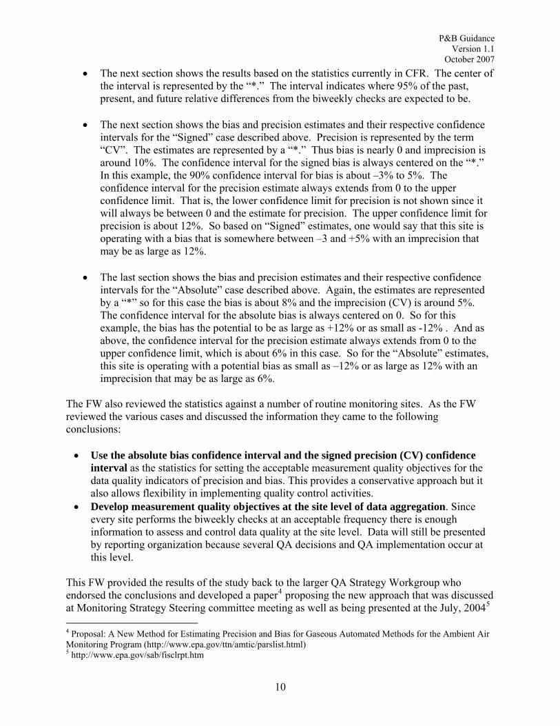
Figure 4 shows the results for one of the hypothetical cases studied. It provides an example of the various precision and bias estimates for a 3 year data set where the true measurement imprecision is 5% and the true bias is 15% for year 1, 0% for year 2 and -10% for year 3. There are 5 sections to the Figure.

Figure 4. Precision and Bias Estimates for a Hypothetical Example

• The left-most area of Figure 4 shows the spread of the relative differences of the

biweekly checks for each of the years and for all the years combined. These box and whisker plots show that the bias varies from year to year and that it is decreasing (the center of boxes shifts from around 15% to 0% to –10%) but that the imprecision is small (the boxes are small and whiskers short). On the other hand, the 3-year box and whisker plot shows no bias (the box is centered about 0) but large variation (the box is wide and the whiskers are long).

• The next section of Figure 4 shows the true bias (represented as *’s) and imprecision

(represented as a line from 0 to the amount of imprecision, 5% in this case).

9


October 2007

• The next section shows the results based on the statistics currently in CFR. The center of the interval is represented by the “*.” The interval indicates where 95% of the past, present, and future relative differences from the biweekly checks are expected to be.

• The next section shows the bias and precision estimates and their respective confidence

intervals for the “Signed” case described above. Precision is represented by the term “CV”. The estimates are represented by a “*.” Thus bias is nearly 0 and imprecision is around 10%. The confidence interval for the signed bias is always centered on the “*.” In this example, the 90% confidence interval for bias is about –3% to 5%. The confidence interval for the precision estimate always extends from 0 to the upper confidence limit. That is, the lower confidence limit for precision is not shown since it will always be between 0 and the estimate for precision. The upper confidence limit for precision is about 12%. So based on “Signed” estimates, one would say that this site is operating with a bias that is somewhere between –3 and +5% with an imprecision that may be as large as 12%.

• The last section shows the bias and precision estimates and their respective confidence

intervals for the “Absolute” case described above. Again, the estimates are represented by a “*” so for this case the bias is about 8% and the imprecision (CV) is around 5%. The confidence interval for the absolute bias is always centered on 0. So for this example, the bias has the potential to be as large as +12% or as small as -12% . And as above, the confidence interval for the precision estimate always extends from 0 to the upper confidence limit, which is about 6% in this case. So for the “Absolute” estimates, this site is operating with a potential bias as small as –12% or as large as 12% with an imprecision that may be as large as 6%.

The FW also reviewed the statistics against a number of routine monitoring sites. As the FW reviewed the various cases and discussed the information they came to the following conclusions: • Use the absolute bias confidence interval and the signed precision (CV) confidence

interval as the statistics for setting the acceptable measurement quality objectives for the data quality indicators of precision and bias. This provides a conservative approach but it also allows flexibility in implementing quality control activities.

• Develop measurement quality objectives at the site level of data aggregation. Since every site performs the biweekly checks at an acceptable frequency there is enough information to assess and control data quality at the site level. Data will still be presented by reporting organization because several QA decisions and QA implementation occur at this level.

This FW provided the results of the study back to the larger QA Strategy Workgroup who endorsed the conclusions and developed a paper4 proposing the new approach that was discussed at Monitoring Strategy Steering committee meeting as well as being presented at the July, 20045

4 Proposal: A New Method for Estimating Precision and Bias for Gaseous Automated Methods for the Ambient Air Monitoring Program (http://www.epa.gov/ttn/amtic/parslist.html) 5 http://www.epa.gov/sab/fisclrpt.htm

10


October 2007 Clean Air Scientific Advisory Committee (CASAC) meeting where the statistics were endorsed. As the QA Strategy Workgroup moved forward in its review of other facets of the ambient air quality system, EPA pursued using similar statistics for the particulate matter parameters. In general, and as the following information will show, EPA has followed a similar path for the majority of the particulate matter measurement quality samples. One exception must be noted. Since DQOs and there accompanying statistics had been developed for PM2.5 shortly before the FW efforts to develop the new statistical techniques, and because EPA was preparing the monitoring rule proposal at a time when PM2.5 design values were being compared to the NAAQS, EPA did not want to modify the bias statistics to the new absolute bias confidence limit technique. Therefore, although the precision statistic for PM2.5 has been changed to be consistent with the gaseous pollutants, the bias estimate for PM2.5 has been maintained as written prior to the 10/17/06 rule. However, for convenience, the companion software for this document will provide an assessment of PM2.5 bias by both statistical methods.

11


October 2007

Section 2: The New Statistics: A Fool-Proof Method & DASC Tool

Section 1 provided a background on the Ambient Air Monitoring program, the use of the precision and accuracy statistics prior to the promulgation of the new statistics in 2006, and an explanation of how the new statistics in the 2006 rule were developed. This section and the companion Data Assessment Statistical Calculator (DASC) tool has been produced specifically for the data user community in an effort to provide an easy way to explain and calculate the new data assessment statistics in CFR. Each equation explained in this document is numbered and matches the numbering convention in CFR! Given measurement quality data for a particular pollutant and site, this section provides a step-by-step way to: (1) know what to calculate and (2) calculate it. The DASC tool can be found under its filename, “P & B DASC”, in the Precision and Accuracy Reporting System within the Quality Assurance section of AMTIC6 and uses data that you input as the basis to perform all calculations outlined in this document. The DASC contains eight (8) different worksheets; one for each of the seven different categories of statistics that need to be calculated, and the eighth being a menu selection tool to help you find the appropriate worksheet. Table 3 illustrates what data quality indicators are applicable for each of the monitored pollutants. Table 3 Data Quality Indicators Calculated for each Measured Pollutant

What to Calculate Pollutants

Pick a Statistic O3 SO2 NO2 CO PM2.5 PM10 PM10-2.5 Lead Precision Estimate Bias Estimate Absolute Bias Estimate Semi-Annual Flow Rate One Point Flow Rate

The titles under the “Pick a Statistic” label correspond to the titles of the worksheets in the DASC. Figure 5 is the “Menu” worksheet. At the menu you can select: 1) the pollutant, and 2) the data quality indicator you want to calculate. Selecting the “Go to Worksheet” button takes you to the worksheet. In the case shown in Figure 5 the user would be taken to the gaseous pollutant precision worksheet for NO2.

Figure 5. DASC main menu

6 http://www.epa.gov/ttn/amtic/parslist.html

12

Final Draft 1/19/07

All measurement quality checks start with a comparison of the concentration/value measured by the analyzer (measured value) and the audit concentration/value (audit value) and all use percent or relative percent difference as the comparison statistic. All other calculations are based on these two “starting” statistics. To create a measurement quality spreadsheet using the DASC tool, put the measured value data in Column A and the corresponding audit value data in Column B. Remember to start the data in Row 4 so that Rows 1-3 are reserved for labels. All subsequent calculations will be automatically generated by the spreadsheet. For those who have used the AQS precision and accuracy transaction files, the measured value equates to the “indicated value” and the audit value equates to the “actual value” The spreadsheet has been created with a pre-defined set of 13 audit pairs to provide an example. These values will need to be replaced by your sample data set. All the formulas in columns C, E, F, and G, from row 4 through row 503 have been preset to calculate the necessary statistics. If you plan to add more than 500 data pairs you will have to revise the excel spreadsheet. Each worksheet allows you to print the data and graphs for that worksheet by using the “print worksheet” button. The pages will be automatically set based on the number of values input. If you would like to print out the entire workbook head back to the main menu.

Please Note The DASC tool contains macros that need to be enabled in order for the spreadsheet to work properly. When you first open the document, you should see a message that looks like this:

Click on “Enable Macros” and the worksheet will open. If you do not get this message, make sure that you have the macro security level setting set to “Medium”. The macro security level setting can be found in “Security” tab from the “Tools” “Options…” menu in Excel

13


October 2007

2.1 Gaseous Precision and Bias Assessments Applies to: CO, O3, NO2, SO2 40 CFR Part 58 Appendix A References:

• 4.1.1 Percent Difference • 4.1.2 Precision Estimate • 4.1.3 Bias Estimate • 4.1.3.1 Assigning a sign (positive / negative) to the bias estimate. • 4.1.3.2 Calculate the 25th and 75th percentiles of the percent differences for each site. • 4.1.4 Validation of Bias Using the one-point QC Checks

Figure 6. Gaseous precision and bias DASC worksheet example Percent Difference Equations from this section come from CFR Pt. 58, App. A, Section 4, “Calculations for Data Quality Assessment”. For each single point check, calculate the percent difference, di, as follows:

Equation 1

where meas is the concentration indicated by the monitoring organization’s instrument and audit is the audit concentration of the standard used in the QC check being measured.

dmeas audit

auditi =−

⋅100

Precision Estimate The precision estimate is used to assess the one-point QC checks for gaseous pollutants described in section 3.2.1 of CFR Part 58, Appendix A. The precision estimator is the coefficient of variation upper bound and is calculated using Equation 2 as follows:

14


October 2007 Equation 2

where χ2 0.1,n-1 is the 10th percentile of a chi-squared distribution with n-1 degrees of freedom. Bias Estimate The bias estimate is calculated using the one point QC checks for SO2, NO2, O3, or CO described in CFR, section 3.2.1. The bias estimator is an upper bound on the mean absolute value of the percent differences as described in Equation 3 as follows:

Equation 3 bias AB t AS

nn= + ⋅−0 95 1. ,

where n is the number of single point checks being aggregated; t0.95,n-1 is the 95th quantile of a t-distribution with n-1 degrees of freedom; the quantity AB is the mean of the absolute values of the di’s (calculated by Equation 1) and is expressed as Equation 4 as follows:

Equation 4

and the quantity AS is the standard deviation of the absolute value of the di’s and is calculated using Equation 5 as follows:

Equation 5

( ) 21,1.0

1

2

1

2

11 −

= = −⋅

−

⎟⎠

⎞⎜⎝

⎛−⋅

=∑ ∑

n

n

i

n

iii n

nn

ddnCV

χ

ABn

d ii

n

= ⋅=∑1

1

( )AS

n d d

n n

ii

n

ii

n

=

⋅ −⎛

⎝⎜⎜

⎞

⎠⎟⎟

−= =∑ ∑2

1 1

2

1

Since the bias statistic as calculated in Equation 3 of this document uses absolute values, it does not have a tendency (negative or positive bias) associated with it. A sign will be designated by rank ordering the percent differences (di’s) of the QC check samples from a given site for a particular assessment interval. Calculate the 25th and 75th percentiles of the percent differences for each site. The absolute bias upper bound should be flagged as positive if both percentiles are positive and negative if both percentiles are negative. The absolute bias upper bound would not be flagged if the 25th and 75th percentiles are of different signs (i.e. straddling zero).

15


October 2007 The final precision value should be found in cell I13 and the final bias estimate should be found in cell K13 in the spreadsheet. See the corresponding spreadsheet (‘P&B DASC.xls’). Validation of Bias Using the one-point QC Checks The annual performance evaluations for SO2, NO2, O3, or CO are used to verify the results obtained from the one-point QC checks and to validate those results across a range of concentration levels. To quantify this annually at the site level and at the 3-year primary quality assurance organization level, probability limits will be calculated from the one-point QC checks using equations 6 and 7:

Equation 6

S1.96mLimityProbabilitUpper ⋅+=

Equation 7

S1.96mLimityProbabilitLower ⋅−= where, m is the mean (equation 8):

Equation 8

∑=

⋅=k

1iid

k1m

where, k is the total number of one point QC checks for the interval being evaluated and S is the standard deviation of the percent differences (equation 9) as follows:

Equation 9

1)-k(k

ddkS

2k

1ii

k

1i

2i ⎟

⎠

⎞⎜⎝

⎛−⋅

=∑∑==

Please Note P&B DASC.xls only calculates the upper and lower confidence limits on a per site basis. A similar procedure would need to take place to calculate the upper and lower confidence limits across a Primary Quality Assurance Organization.

16


October 2007

2.2 Precision Estimates from Collocated Samples Applies to: PM2.5, PM10, PM10-2.5, Lead 40 CFR Part 58 Appendix A References:

• 4.2.1 Precision Estimate from Collocated Samplers • 4.3.1 Precision Estimate(PM2.5 & PM10-2.5) • 4.4.1 Precision Estimate (Lead)

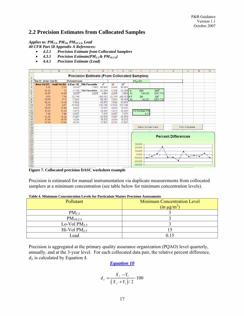
Figure 7. Collocated precision DASC worksheet example Precision is estimated for manual instrumentation via duplicate measurements from collocated samplers at a minimum concentration (see table below for minimum concentration levels). Table 4. Minimum Concentration Levels for Particulate Matter Precision Assessments

Pollutant Minimum Concentration Level (in μg/m3)

PM2.5 3 PM10-2.5 3

Lo-Vol PM2.5 3 Hi-Vol PM2.5 15

Lead 0.15 Precision is aggregated at the primary quality assurance organization (PQAO) level quarterly, annually, and at the 3-year level. For each collocated data pair, the relative percent difference, di, is calculated by Equation 4.

Equation 10

( )d

X YX Yi

i i

i i=

−+

⋅/ 2

100

17


October 2007

where Xi is the concentration of the primary sampler and Yi is the concentration value from the audit sampler.

The precision upper bound statistic, CVub, is a standard deviation on di with a 90 percent upper confidence limit (Equation 11).

Equation 11

( ) 21,1.0

2

1

2

1 112

_−

== −⋅

−

⎟⎠

⎞⎜⎝

⎛−⋅

=∑∑

n

n

ii

n

ii n

nn

ddnubCV

χ

where, n is the number of valid data pairs being aggregated, and χ20.1,n-1 is the 10th percentile of a

chi-squared distribution with n-1 degrees of freedom. The factor of 2 in the denominator adjusts for the fact that each di is calculated from two values with error.

18


October 2007

2.3 PM2.5 Bias Assessment Applies to: PM2.5 40 CFR Part 58 Appendix A Reference:

• 4.3.2 Bias Estimate (PM2.5)

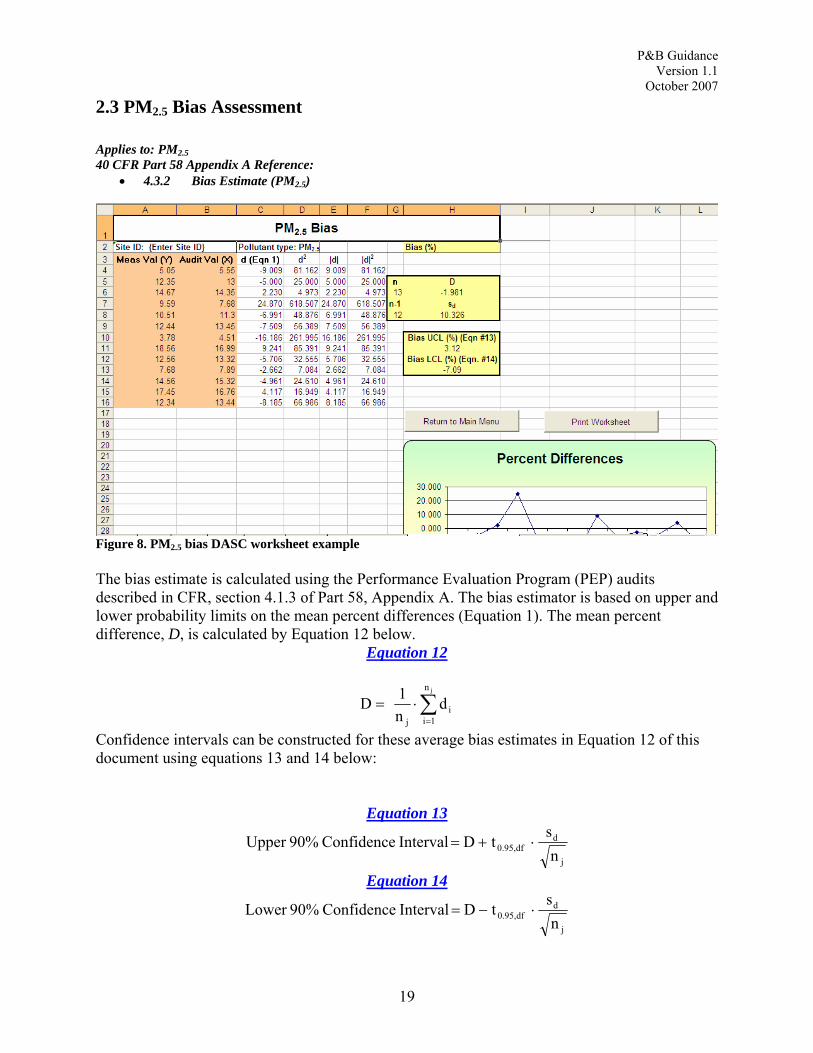
Figure 8. PM2.5 bias DASC worksheet example The bias estimate is calculated using the Performance Evaluation Program (PEP) audits described in CFR, section 4.1.3 of Part 58, Appendix A. The bias estimator is based on upper and lower probability limits on the mean percent differences (Equation 1). The mean percent difference, D, is calculated by Equation 12 below.

Equation 12

∑=

⋅=jn

1ii

j

dn1D

Confidence intervals can be constructed for these average bias estimates in Equation 12 of this document using equations 13 and 14 below:

Equation 13

j

ddf0.95, n

stDIntervalConfidence90%Upper ⋅+=

Equation 14

j

ddf0.95, n

stDIntervalConfidence90%Lower ⋅−=

19


October 2007 Where, t0.95,df is the 95th quantile of a t-distribution with degrees of freedom df=nj-1 and sd is an estimate of the variability of the average bias and is calculated using Equation 15 below:

Equation 15

( )

1n

ds

j

1i

2i

d −

−=∑=

jn

D

20


October 2007

2.4 PM 10-2.5 and PM2.5 Absolute Bias Assessment Applies to: PM10-2.5 and PM2.5 (for estimation purposes only) 40 CFR Part 58 Appendix A Reference:

• 4.1.3 Bias Estimate (PM10-2.5)

Figure 9. PM2.5 absolute bias DASC worksheet example (PM10-2.5 is virtually the same) The bias estimate is calculated using the Performance Evaluation Program (PEP) audits described in CFR, section 4.1.3 of Part 58, Appendix A. The bias estimator is an upper bound on the mean absolute value of the percent differences (Equation 1), as described in Equation 3 as follows:

Equation 3

where n is the number of PEP audits being aggregated; t0.95,n-1 is the 95th quantile of a t-distribution with n-1 degrees of freedom; the quantity AB is the mean of the absolute values of the di’s (calculated by Equation 1) and is expressed as Equation 4 as follows:

Equation 4

bias AB t ASn

n= + ⋅−0 95 1. ,

ABn

d ii

n

= ⋅=∑1

1

and the quantity AS is the standard deviation of the absolute value of the di’s (Equation 1) and is calculated using Equation 5 as follows:

21



( )AS

n d d

n n

ii

n

ii

n

=

⋅ −⎛

⎝⎜⎜

⎞

⎠⎟⎟

−= =∑ ∑2

1 1

2

1

Since the bias statistic as calculated in Equations 3 and 6 of this document uses absolute values, it does not have a sign direction (negative or positive bias) associated with it. A sign will be designated by rank ordering the percent differences of the QC check samples from a given site for a particular assessment interval. Calculate the 25th and 75th percentiles of the percent differences for each site. The absolute bias upper bound should be flagged as positive if both percentiles are positive and negative if both percentiles are negative. The absolute bias upper bound would not be flagged if the 25th and 75th percentiles are of different signs (i.e. straddling zero).

22


October 2007

2.5 One-Point Flow Rate Bias Estimate Applies to: PM10, PM2.5, PM10-2.5 40 CFR Part 58 Appendix A References:

• 4.2.2 Bias Estimate Using One-Point Flow Rate Verifications (PM10) • 4.3.2 Bias Estimate (PM10-2.5) • Assigning a sign (positive / negative) to the bias estimate.

Figure 10. One-point flow rate DASC worksheet example The bias estimate is calculated using the collocated audits previously described. The bias estimator is an upper bound on the mean absolute value of the percent differences (Equation 1), as described in Equation 3 as follows:

Equation 3

where n is the number of flow audits being aggregated; t0.95,n-1 is the 95th quantile of a t-distribution with n-1 degrees of freedom; the quantity AB is the mean of the absolute values of the di’s (calculated by Equation 4) and is expressed as Equation 4 as follows:

Equation 4

bias AB t ASn

n= + ⋅−0 95 1. ,

ABn

d ii

n

= ⋅=∑1

1

23


October 2007 and the quantity AS is the standard deviation of the absolute value of the di’s (Equation 4) and is calculated using Equation 5 as follows:

Equation 5

( )AS

n d d

n n

ii

n

ii

n

=

⋅ −⎛

⎝⎜⎜

⎞

⎠⎟⎟

−= =∑ ∑2

1 1

2

1

Since the bias statistic as calculated in Equation 3 of this document uses absolute values, it does not have a sign direction (negative or positive bias) associated with it. A sign will be designated by rank ordering the percent differences of the QC check samples from a given site for a particular assessment interval. Calculate the 25th and 75th percentiles of the percent differences for each site. The absolute bias upper bound should be flagged as positive if both percentiles are positive and negative if both percentiles are negative. The absolute bias upper bound would not be flagged if the 25th and 75th percentiles are of different signs (i.e. straddling zero).

24


October 2007

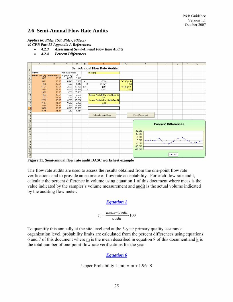
2.6 Semi-Annual Flow Rate Audits Applies to: PM10, TSP, PM2.5, PM10-2.540 CFR Part 58 Appendix A References:

• 4.2.3 Assessment Semi-Annual Flow Rate Audits • 4.2.4 Percent Differences

Figure 11. Semi-annual flow rate audit DASC worksheet example The flow rate audits are used to assess the results obtained from the one-point flow rate verifications and to provide an estimate of flow rate acceptability. For each flow rate audit, calculate the percent difference in volume using equation 1 of this document where meas is the value indicated by the sampler’s volume measurement and audit is the actual volume indicated by the auditing flow meter.

Equation 1

dmeas audit

auditi =−

⋅100

To quantify this annually at the site level and at the 3-year primary quality assurance organization level, probability limits are calculated from the percent differences using equations 6 and 7 of this document where m is the mean described in equation 8 of this document and k is the total number of one-point flow rate verifications for the year

Equation 6

S1.96mLimityProbabilitUpper ⋅+=

25



S1.96mLimityProbabilitLower ⋅−=

where, m is the mean (equation 8):

Equation 8

∑=

⋅=k

1iid

k1m

where, k is the total number of one point QC checks for the interval being evaluated and S is the standard deviation of the percent differences (equation 9) as follows:

Equation 9

1)-k(k

ddkS

2k

1ii

k

1i

2i ⎟

⎠

⎞⎜⎝

⎛−⋅

=∑∑==

26


October 2007

2.7 Lead Bias Assessments Applies to: Lead 40 CFR Part 58 Appendix A References:

• 4.4.2 Bias Estimate (Lead) o 4.4.2.1 Flow Rate Audit (“volume bias”) Calculations o 4.4.2.2 Lead Strip (“mass bias”) Calculations o 4.4.2.3 Final Bias Calculations

Figure 12 - Lead Bias DASC worksheet example In order to estimate bias, the information from the flow rate audits and the Pb strip audits needs to be combined as described below. To be consistent with the formulas for the gases, the recommended procedures are to work with relative errors of the lead measurements. The relative error in the concentration is related to the relative error in the volume and the relative error in the mass measurements using Equation 16 of this appendix:

Equation 16

( )ionconcentrataudit

ionconcentratauditionconcentratmeasurederrorrel. −=

( )errorvolumerel.errormassrel.rel.error1

1−⎟⎟

⎠

⎞⎜⎜⎝

⎛+

=

As with the gases, an upper bound for the absolute bias is desired. Using Equation 16 above, the absolute value of the relative (concentration) error is bounded by equation 17 of this appendix:

27


October 2007

Equation 17

errorvolumerelative1errorvolumerelativeerrormassrelative

errorrel.−

+≤

The quality indicator data collected are then used to bound each part of Equation 17 separately. “Flow Audit” calculations. For each flow rate audit, calculate the percent difference, di,, in volume by Equation 1 of this appendix where meas is the value indicated by the sampler’s volume measurement and audit is the actual volume indicated by the auditing flow meter.

Equation 1

dmeas audit

auditi =−

⋅100

The absolute “volume bias” upper bound is then calculated using Equation 3 of this appendix where n is the number of flow rate audits being aggregated; t0.95,n-1 is the 95th quantile of a t-distribution with n-1 degrees of freedom; the quantity AB is the mean of the absolute values of the di’s and is calculated using Equation 4, and the quantity AS in Equation 3 of this appendix is the standard deviation of the absolute values of the di’s and is calculated using Equation 5 of this appendix.

Equation 3

bias AB t AS

nn= + ⋅−0 95 1. ,


Equation 4

AB

nd i

i

n

= ⋅=∑1

1


Equation 5

28( )

ASn n

i i=−

= =1 1

1

n d di

n

i

n

⋅ −⎛

⎝⎜⎜

⎞

⎠⎟⎟∑ ∑2

2


October 2007 “Pb Strip Audit”calculations. Similarly for each lead strip audit, calculate the percent difference, di, in mass by Equation 1 where meas is the value indicated by the mass measurement and audit is the actual lead mass on the audit strip.

Equation 1

dmeas audit

auditi =−

⋅100

The absolute “mass bias” upper bound is then calculated using Equation 3 of this appendix where n is the number of lead strip audits being aggregated; t0.95,n-1 is the 95th quantile of a t-distribution with n-1 degrees of freedom;

Equation 3

bias AB t AS

nn= + ⋅−0 95 1. ,


Equation 4

AB

nd i

i

n

= ⋅=∑1

1


Equation 5

( )AS

n d d

n n

ii

n

ii

n

=

⋅ −⎛

⎝⎜⎜

⎞

⎠⎟⎟

−= =∑ ∑2

1 1

2

1

Final |Bias| Calculation. Finally, the absolute bias upper bound is given by combining the absolute bias estimates of the flow rate and Pb strips using Equation 18 of this appendix:

29



100bias vol.100

bias vol.bias massbias ⋅

−

+=

where mass bias is the bias calculated for the Pb strips, and vol is the bias calculated for the flow rate audits. The numerator and denominator have been multiplied by 100 for expression in percent. Since the bias statistic as calculated in Equation 3 of this document uses absolute values, it does not have a sign direction (negative or positive bias) associated with it. A sign will be designated by rank ordering the percent differences of the QC check samples from a given site for a particular assessment interval. Calculate the 25th and 75th percentiles of the percent differences for each site. The absolute bias upper bound should be flagged as positive if both percentiles are positive and negative if both percentiles are negative. The absolute bias upper bound would not be flagged if the 25th and 75th percentiles are of different signs (i.e. straddling zero). Time Period for Audits. The statistics in this section assume that the mass and flow rate audits represent the same time period. Since the two types of audits are not performed at the same time, the audits need to be grouped by common time periods. Consequently, the absolute bias estimates should be done on annual and 3-year levels. The flow rate audits are site-specific, so the absolute bias upper bound estimate can be done and treated as a site-level statistic.

30

31

Page intentionally left blank

32

lease read Instructions on reverse before com

TECHNICAL REPORT DATA (P pleting) 1. REPORT NO. EPA-454/B-07-001

3. RECIPIENT'S ACCESSION NO. 2.

5. REPORT DATE : January, 2007

4. TITLE AND SUBTITLE

ecision and Bias Data equired by 40 CFR Part 58 Appendix A

PERFORMING ORGANIZATION CODE

Guideline on the Meaning and the Use of PrR

6.

7.

AUTHOR(S) Louise Camalier, Shelly Eberly Jonathan Miller , Michael Papp

PERFORMING ORGANIZATION REPORT NO.

8.

10. PROGRAM ELEMENT NO.

9. PERFORMING ORGANIZATION NAME AND ADDRESS Office of Air Quality Planning and Standa

rds

cy GRANT NO.

U.S. Environmental Protection Agen Research Triangle Park, NC 27711

11. CONTRACT/

13. TYPE OF REPORT AND PERIOD COVERED

12. SPONSORING AGENCY NAME AND ADDRESS

ards

, NC 27711

ENCY CODE EPA/200/04

Office of Air Quality Planning and Stand U.S. Environmental Protection Agency Research Triangle Park

14. SPONSORING AG

15. SUPPLEMENTARY NOTES

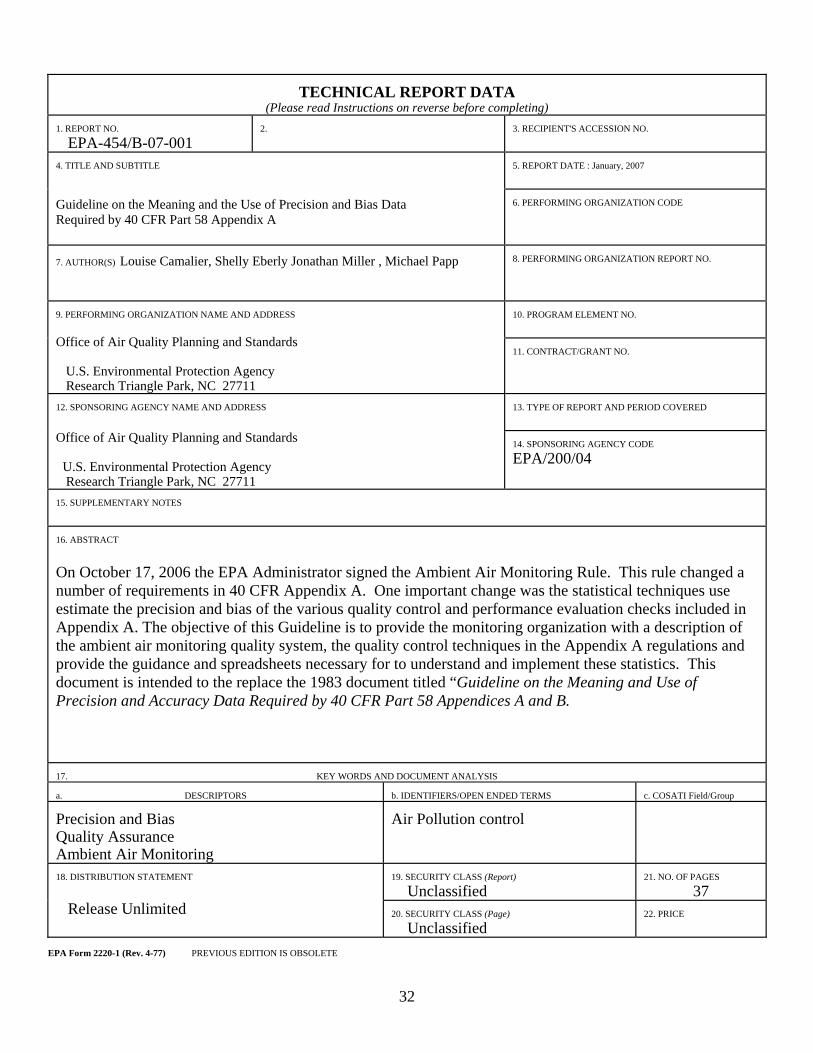
16. ABSTRACT

a

nd is

eaning and Use of recision and Accuracy Data Required by 40 CFR Part 58 Appendices A and B.

On October 17, 2006 the EPA Administrator signed the Ambient Air Monitoring Rule. This rule changed number of requirements in 40 CFR Appendix A. One important change was the statistical techniques use estimate the precision and bias of the various quality control and performance evaluation checks included in Appendix A. The objective of this Guideline is to provide the monitoring organization with a description of the ambient air monitoring quality system, the quality control techniques in the Appendix A regulations aprovide the guidance and spreadsheets necessary for to understand and implement these statistics. Thdocument is intended to the replace the 1983 document titled “Guideline on the MP 17. KEY WORDS AND DOCUMENT ANALYSIS a. DESCRIPTORS RMS COSATI Field/Group b. IDENTIFIERS/OPEN ENDED TE c.

Precision and Bias Quality Assurance Ambient Air Monitoring

ir Pollution control

A

19. SECURITY CLASS (Report) 37 Unclassified

21. NO. OF PAGES

18. DISTRIBUTION STATEMENT

Release Unlimited ge) Unclassified

22. PRICE 20. SECURITY CLASS (Pa

EPA Form 2220-1 (Rev. 4-77) PREVIOUS EDITION IS OBSOLETE

guideline on the meaning and the use of precision and bias...

Documents