guide to equilibrium dialysis - the nest group · guide to equilibrium dialysis 1 introduction ......

Guide toEquilibriumDialysis

AcknowledgementThe sections of this booklet about mass-action and regression wereadapted, with permission, from H.J. Motulsky, Analyzing Data withGraphPad Prism, GraphPad Software, 1999. Additional information isavailable on line at www.curvefit.com.

© All text, photographs and illustrations are copyrighted by Harvard Bioscience,Inc. 2002. Product names Micro-Equilibrium Dialyzer™, Dispo-EquilibriumDialyzer™, Equilibrium Dialyzer-96™ and Multi-Equilibrium Dialyzer™ are trade-marks of Harvard Apparatus, Inc.

Distributed by:

The Nest Group, Inc.45 Valley RoadSouthborough, MA 01772-1323

Phone: (800) 347-6378 or 508-481-6223Fax: (508) 485-5736Web: www.nestgrp.comE-mail: [email protected]

Guide to Equilibrium Dialysis 1

Introduction ............................................................................2

Protocol ..................................................................................3

Analysis....................................................................................5

Analysis of Ligand Binding Data ....................................6

Linear Regression ..................................................................10

Introduction to Linear Regression ................................10

The ScatchardPlot ........................................................10

Analysis ........................................................................11

Non-Linear Regression ..........................................................13

Introduction to Non-Linear Regression ........................13

Sum-of-Squares..............................................................14

Analysis ........................................................................14

Example ................................................................................18

Additional Reading ................................................................20

Products

Dispo-Equilibrium Dialyzer™ ........................................21

Micro-Equilibrium Dialyzer™ ........................................22

Equilibrium Dialyzer-96™..............................................24

Plate Rotator ................................................................25

Multi-Equilibrium Dialyzer™ ........................................26

Graphpad Prism® ..........................................................28

Contents

Harvard Bioscience2

IntroductionEquilibrium Dialysis is a simple but effective tool for the study of interac-tions between molecules. Whether it be characterization of a candidatedrug in serum binding assays or detailed study of antigen-antibody interac-tions, equilibrium dialysis proves to be the most accurate method available.Equilibrium dialysis is inexpensive and easy to perform, the only instru-mentation required is that used to quantify the compound of interest.Since the results of the assay are obtained under equilibrium conditions,the true nature of the interaction can be studied. Equilibrium dialysis alsooffers the ability to study low affinity interactions that are undetectableusing other methods.

This guide offers an introduction to the technique of equilibrium dialysisand some examples of how this technique can be used in real world appli-cations. There is also an introduction to the types of data analysis methodsused to extract results from these types of experiments. Details of the widerange of equilibrium dialysis products offered by Harvard Bioscience canbe found towards the back of this booklet.


ProtocolIn a standard equilibrium dialysisassay you begin with two chambersseparated by a dialysis membrane.The molecular weight cut off(MWCO) of this membrane ischosen such that it will retain thereceptor component of the sample(the element which will bind the ligand).

A known concentration and vol-ume of ligand is placed into one ofthe chambers. The ligand is smallenough to pass freely through themembrane.

A known concentration of receptoris then placed in the remainingchamber in an equivalent volumeto that placed in the first chamber.

As the ligand diffuses across themembrane some of it will bind tothe receptor and some will remainfree in solution. The higher theaffinity of the interaction, the high-er the concentration of ligand thatwill be bound at any time.

Diffusion of the ligand across themembrane and binding of the ligand continues until equilibriumhas been reached. At equilibrium,the concentration of ligand free insolution is the same in both cham-bers. In the receptor chamber,however, the overall concentrationis higher due to the bound-ligandcomponent.

The concentration of free ligand in the ligand chamber can then be usedto determine the binding characteristics of the samples as described in thenext section.

Harvard Bioscience4

At Equilibrium

Sample Chamber Assay Chamber

Analysis


Equilibrium Dialysis can be used in a wide variety of experiments and themethods used to analyze the resulting data can vary just as widely. Thissection serves as an introduction to the types of data analysis tools used tointerpret experimental data generated using equilibrium dialysis.

The type of assay typically performed using equilibrium dialysis falls underthe category of saturation binding experiments. In this case the equilibri-um binding of various concentrations of the receptor and ligand is meas-ured. The relationship between binding and ligand concentration is thenused to determine the number of binding sites, Bmax, and the ligand affin-ity, kd. Because this kind of experimental data used to be analyzed withScatchard plots, they are sometimes called “Scatchard experiments”.

Harvard Bioscience6

Analysis of Ligand Binding Data

Analysis of ligand binding experiments is based on a simple model, calledthe law of mass action. This model assumes that binding is reversible.

Binding occurs when ligand and receptor collide due to diffusion, andwhen the collision has the correct orientation and enough energy. The rateof association is:

[ ] denotes concentration

The association rate constant (kon) is expressed in units of M-1min-1 .Once binding has occurred, the ligand and receptor remain bound togeth-er for a random amount of time. The probability of dissociation is thesame at every instant of time. The receptor doesn’t “know” how long it hasbeen bound to the ligand. The rate of dissociation is:

The dissociation constant koff is expressed in units of min-1. After dissoci-ation, the ligand and receptor are the same as at they were before binding.If either the ligand or receptor is chemically modified, then the bindingdoes not follow the law of mass action. Equilibrium is reached when therate at which new ligand-receptor complexes are formed equals the rate atwhich the ligand-receptor complexes dissociate. At equilibrium:


Variable Name Units

kon Association rate constant or on-rate constant M-1min-1

koff Dissociation rate constant or off-rate constant min-1

kd Equilibrium dissociation constant M

Rearrange that equation to define the equilibrium dissociation constant kd.Define the equilibrium dissociation constant, kd to equal koff/kon, whichis in molar units. In enzyme kinetics, this is called the Michaelis-Mentenconstant, KM.

The kd has a meaning that is easy to understand. Set [Ligand] equal to kdin the equation above. The kd terms cancel out, and you’ll see that[Receptor]/[Ligand • Receptor]=1, so [Receptor] equals [Ligand •Receptor]. Since all the receptors are either free or bound to ligand, thismeans that half the receptors are free and half are bound to ligand. Inother words, when the concentration of ligand equals the kd, half thereceptors will be occupied at equilibrium. If the receptors have a highaffinity for the ligand, the kd will be low, as it will take a low concentra-tion of ligand to bind half the receptors.

Don’t mix up kd, the equilibrium dissociation constant, with koff, the dis-sociation rate constant. They are not the same, and aren’t even expressed inthe same units.

Harvard Bioscience8

[Ligand] Fractional Occupancy

0 0

1 • kd 50%

4 • kd 80%

9 • kd 90%

99 • kd 99%

Fractional occupancy is the fraction of all receptors that are bound to ligand.

This equation can be more clearly represented as:

This equation assumes equilibrium. To make sense of it, think about a fewdifferent values for [Ligand].

This becomes even clearer in graphical form.

Note that when [Ligand]=kd, fractional occupancy is 50%.

Fractional Occupancy =[Ligand]

[Ligand]+Kd


Although termed a “law”, the law of mass action is simply a model thatcan be used to explain some experimental data. Because it is so simple, themodel is not useful in all situations. The model assumes:

– All receptors are equally accessible to ligands.– Receptors are either free or bound to ligand. It doesn’t allow

for more than one affinity state, or states of partial binding.– Binding does not alter the ligand or receptor.– Binding is reversible.

Despite its simplicity, the law of mass action has proven to be very usefulin describing many aspects of receptor pharmacology and physiology.

Linear Regression

Harvard Bioscience10

Linear Regression: Introduction

In the days before nonlinear regression programs (eg. Graphpad Prism)were widely available,scientists transformed data into a linear form, andthen analyzed the data by linear regression.

Linear regression analyzes the relationship between two variables, X and Y.For each subject (or experimental unit), you know both X and Y and youwant to find the best straight line through the data. In some situations, theslope and/or intercept have a scientific meaning. In other cases, you use thelinear regression line as a standard curve to find new values of X from Y, orY from X. In general, the goal of linear regression is to find the line thatbest predicts Y from X. Linear regression does this by finding the line thatminimizes the sum of the squares of the vertical distances of the pointsfrom the line.

Linear Regression: The Scatchard Plot

There are several ways to linearize binding data, including the methods ofLineweaver-Burke and Eadie-Hofstee. However, the most popular methodto linearize binding data is to create a Scatchard plot, as shown in the rightpanel below.


In this plot, the X-axis is specific binding and the Y-axis is specific bindingdivided by free ligand concentration. It is possible to estimate the Bmaxand kd from a Scatchard plot (Bmax is the X intercept; kd is the negativereciprocal of the slope). However, the Scatchard transformation distorts theexperimental error, and thus violates several assumptions of linear regres-sion. The Bmax and kd values you determine by linear regression ofScatchard transformed data may be far from their true values.

Linear Regression: Analysis

The problem with this method is that the transformation distorts theexperimental error. Linear regression assumes that the scatter of pointsaround the line follows a Gaussian distribution and that the standard devi-ation is the same at every value of X. These assumptions are rarely trueafter transforming data. Furthermore, some transformations alter the rela-tionship between X and Y. For example, in a Scatchard plot the value of X(bound) is used to calculate Y (bound/free), and this violates the assump-tion of linear regression that all uncertainty is in Y while X is known pre-cisely. It doesn’t make sense to minimize the sum of squares of the verticaldistances of points from the line, if the same experimental error appears inboth X and Y directions. Since the assumptions of linear regression areviolated, the values derived from the slope and intercept of the regressionline are not the most accurate determinations of the variables in the model.Considering all the time and effort you put into collecting data, you wantto use the best possible technique for analyzing your data. Nonlinearregression produces the most accurate results.

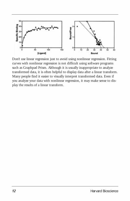
The graph below shows the problem of transforming data. The left panelshows data that follows a rectangular hyperbola (binding isotherm). Theright panel is a Scatchard plot of the same data. The solid curve on the leftwas determined by nonlinear regression. The solid line on the right showshow that same curve would look after a Scatchard transformation. Thedotted line shows the linear regression fit of the transformed data.Scatchard plots can be used to determine the receptor number (Bmax,determined as the X-intercept of the linear regression line) and dissociationconstant (kd, determined as the negative reciprocal of the slope). Since theScatchard transformation amplified and distorted the scatter, the linearregression fit does not yield the most accurate values for Bmax and kd.


Don’t use linear regression just to avoid using nonlinear regression. Fittingcurves with nonlinear regression is not difficult using software programssuch as Graphpad Prism. Although it is usually inappropriate to analyzetransformed data, it is often helpful to display data after a linear transform.Many people find it easier to visually interpret transformed data. Even ifyou analyze your data with nonlinear regression, it may make sense to dis-play the results of a linear transform.

Non-Linear Regression


Non-Linear Regression: Introduction

Linear regression is described in every statistics book, and is performed byevery statistics program. Nonlinear regression is mentioned in only a fewbooks, and is not performed by all statistics programs. From a mathemati-cian’s point of view, the two procedures are vastly different. From a scien-tist’s point of view, however, the two procedures are very similar. In manyfields of science, nonlinear regression is used far more often than linearregression. A line is described by a simple equation that calculates Y fromX, slope and intercept. The purpose of linear regression is to find values forthe slope and intercept that define the line that comes closest to the data.More precisely, it finds the line that minimizes the sum of the square ofthe vertical distances of the points from the line. The equations used to dothis can be derived with no more than high-school algebra (shown in manystatistics books). Put the data in, and the answers come out. There is nochance for ambiguity. You could even do the calculations by hand, if youwanted to.

Nonlinear regression is more general than linear regression. It fits data toany equation that defines Y as a function of X and one or more parame-ters. It finds the values of those parameters that generate the curve thatcomes closest to the data. More precisely, nonlinear regression finds thevalues of the parameters that generates a curve that minimizes the sum ofthe squares of the vertical distances of the data points from the curve.

Except for a few special cases, it is not possible to directly derive an equa-tion to compute the best-fit values from the data. Instead nonlinear regres-sion requires a computationally intensive, iterative approach. You can’t real-ly follow the mathematics of nonlinear regression unless you are familiarwith matrix algebra. But these complexities only pertain to performing thecalculations, which can be performed easily with non-linear regression soft-ware (like GraphPad Prism). Using nonlinear regression to analyze data isonly slightly more difficult than using linear regression. Your choice of lin-ear or nonlinear regression should be based on the model you are fitting.Don’t use linear regression just to avoid using nonlinear regression.


Non-Linear Regression: Sum-of-Squares

The goal of nonlinear regression is to adjust the values of the variables inthe model to find the curve that best predicts Y from X. More precisely,the goal of regression is to minimize the sum of the squares of the verticaldistances of the points from the curve. Why minimize the sum of thesquares of the distances? Why not simply minimize the sum of the actualdistances?

If the random scatter follows a Gaussian distribution, it is far more likelyto have two medium size deviations (say 5 units each) than to have onesmall deviation (1 unit) and one large (9 units). A procedure that mini-mized the sum of the absolute value of the distances would have no prefer-ence over a curve that was 5 units away from two points and one that was1 unit away from one point and 9 units from another. The sum of the dis-tances (more precisely, the sum of the absolute value of the distances) is 10units in each case. A procedure that minimizes the sum of the squares ofthe distances prefers to be 5 units away from two points (sum-of-squares =25) rather than 1 unit away from one point and 9 units away from another(sum-of-squares = 82). If the scatter is Gaussian (or nearly so), the curvedetermined by minimizing the sum-of-squares is most likely to be correct.

Non-Linear Regression: Analysis

While the mathematical details of non-linear regression are quite compli-cated, the basic idea is pretty easy to understand. Every nonlinear regres-sion method follows these steps:

1. Start with an initial estimated value for each variable in the equation.

2. Generate the curve defined by the initial values. Calculate the sum-of-squares (the sum of the squares of the vertical distancesof the points from the curve).

3. Adjust the variables to make the curve come closer to the datapoints. There are several algorithms for adjusting the variables, asexplained below.

4. Adjust the variables again so that the curve comes even closer tothe points. Repeat.


5. Stop the calculations when the adjustments make virtually no difference in the sum-of-squares.

6. Report the best-fit results. The precise values you obtain willdepend in part on the initial values chosen in step 1 and the stopping criteria of step 5. This means that repeat analyses of thesame data will not always give exactly the same results.

Step 3 is the only difficult one. Prism (and most other nonlinear regressionprograms) uses the method of Marquardt and Levenberg, which blendstwo other methods, the method of linear descent and the method ofGauss-Newton.

The best way to understand these methods is to follow an example. Hereare some data to be fit to a typical binding curve (rectangular hyperbola).

You want to fit a binding curve to determine Bmax and kd using the equation:


How can you find the values of Bmax and kd that fit the data best? You cangenerate an infinite number of curves by varying Bmax and kd. For each of thegenerated curves, you can compute the sum-of-squares to assess how well thatcurve fits the data. The following graph illustrates the situation.

The X- and Y-axes correspond to two variables to be fit by nonlinearregression (Bmax and kd in this example). The Z-axis is the sum-of-squares. Each point on the surface corresponds to one possible curve. Thegoal of nonlinear regression is to find the values of Bmax and kd that makethe sum-of-squares as small as possible (to find the bottom of the valley).

The method of linear descent follows a very simple strategy. Starting fromthe initial values try increasing each parameter a small amount. If the sum-of-squares goes down, continue. If the sum-of-squares goes up, go backand decrease the value of the parameter instead. You’ve taken a step downthe surface. Repeat many times. Each step will usually reduce the sum-of-squares. If the sum-of-squares goes up instead, the step must have been solarge that you went past the bottom and back up the other side. If thishappens, go back and take a smaller step. After repeating these steps manytimes, you’ll reach the bottom.


The Gauss-Newton method is a bit harder to understand. As with themethod of linear descent, start by computing how much the sum-of-squares changes when you make a small change in the value of eachparameter.

This tells you the slope of the sum-of-squares surface at the point definedby the initial values. If the equation really were linear, this is enough infor-mation to determine the shape of the entire sum-of-squares surface, andthus calculate the best-fit values of Bmax and kd in one step. With a linearequation, knowing the slope at one point tells you everything you need toknow about the surface, and you can find the minimum in one step. Withnonlinear equations, the Gauss-Newton method won’t find the best-fit val-ues in one step, but that step usually improves the fit. After repeatingmany iterations, you reach the bottom.

This method of linear descent tends to work well for early iterations, butworks slowly when it gets close to the best-fit values (and the surface isnearly flat). In contrast, the Gauss-Newton method tends to work badly inearly iterations, but works very well in later iterations. The two methodsare blended in the method of Marquardt (also called the Levenberg-Marquardt method). It uses the method of linear descent in early iterationsand then gradually switches to the Gauss-Newton approach. GraphpadPrism, like most programs, uses the Marquardt method for performingnonlinear regression.

Example


B=[Ligand]bound

[Protein]total

The following example is one possible method of analysis for data from aligand binding experiment.

In this experiment, 1ml samples of a 50,000 Da Protein (5.0 mg/ml) areallowed to come to equilibrium with 1ml volumes of a ligand solution ofseveral concentrations. The concentrations of the ligand solutions used inthe experiment are shown in the table below ([Ligand]total).

[Ligand]total (mmol) [Ligand]free (mmol) [Ligand]bound (mmol)

0.01 0.005 0.0050.02 0.011 0.0090.05 0.030 0.0200.08 0.046 0.0290.10 0.062 0.0380.15 0.104 0.0460.20 0.143 0.0570.40 0.332 0.0680.70 0.623 0.0771.00 0.922 0.0781.25 1.170 0.080

Once equilibrium has been reached the concentration of free ligand ismeasured ([Ligand]free) and the concentration of bound ligand can bedetermined ([Ligand]bound). The experimental results for this exampleare presented in the table above.

At this stage in the experiment a decision must be made regarding how theexperimental data will be analyzed. In this case we will plot a bindingisotherm of the data, use non-linear regression to find the best-fit line forthis data (and hence determine Bmax and Kd). For ease of visual interpre-tation we will then perform a Scatchard transformation on the resultantbest-fit line data.

Generating a binding isotherm for this data involves plotting ligand con-centration ([Ligand]free) in millimoles on the X-axis against binding coeffi-cient (B) on the Y-axis. The binding coefficient is given by:


We then use non-linear regression (Graphpad Prism) tofind the best-fit line for the data.

The concentration of protein is the same in each case, 0.1 mmol.

[Ligand]free (mmol) Binding Coefficient0.005 0.05000.011 0.09000.030 0.20000.046 0.29000.062 0.38000.104 0.46000.143 0.57000.332 0.68000.623 0.77000.922 0.78001.170 0.8000

This can then be plotted:

When using a software package such as Prism, Bmax and Kd are deter-mined automatically. When this facility is not available it is possible todetermine these values from a Scatchard plot, although this will be lessaccurate (as discussed in the linear regression section). The data obtainedfrom the non-linear regression can be put through a Scatchard transforma-tion to generate a linear plot.

The equation of this line is given by:

y = -11.61x + 10.03

Binding Isotherm

To learn more about how nonlinear regression works, we recommend reading:

96 Well Equilibrium Dialyzer™

Kariv I., Cao H., Oldengurg K, (May 2001) Development of a HighThroughput Equilibrium Dialysis Method. Journal of PharmaceuticalSciences Vol. 90, No,5, 580-587.

Dispo Equilibrium Dialyzer™

Three-dimensional Structure of Guanylyl Cyclase Activating Protein-2, aCalcium-sensitive Modulator of Photoreceptor Guanylyl Cyclases James B.Ames, Alexander M. Dizhoor, Mitsuhiko Ikura, Krzysztof Palczewski, andLubert Stryer the journal of biological chemistry Vol. 274, No. 27, Issue ofJuly 2, pp. 19329-19337, 1999

Chapter 15 of Numerical Recipes in C, Second Edition, WH Press, et. Al.,Cambridge Press, 1992.

Chapter 10 of Primer of Applied Regression and Analysis of Variance, SA Glantz and BK Slinker, McGraw-Hill, 1990.

Analyzing Data with GraphPad Prism, H.J. Motulsky, GraphPad Software,1999. Available at www.graphpad.com.

Additional Reading


The Scatchard equation is:

B/L = n/Kd - B/Kd

Where: B = [Ligand]bound/[Protein]total

L = [Ligand]free

n = number of ligands/macromolecule, i.e.thestoichiometry

Kd = the dissociation constant

Thus Kd can be determined as the negative reciprocal of the slope of theline and Bmax is given by the X-intercept.

In this case Kd is 0.086 mmol (8.6 x 10-5M) and Bmax is 0.864.

Products


Dispo-Equilibrium Dialyzer™

Harvard/AmiKa’s Dispo-Equilibrium Dialyzer is a single-use product forinteraction studies. The Dispo-Equilibrium Dialyzer is leak-proof and pro-vides high sample recovery (almost 100 percent). This system is designedfor one-time use with samples such as radiolabeled compounds, avoidingthe hassle associated with cleaning the dialyzer after use. Each chamber has a capacity of up to 75µl. The Dispo-EquilibriumDialyzer utilizes high-quality regenerated cellulose membranes withMWCO’s of 5,000 or 10,000 Daltons. Sample recovery is very easythrough centrifugation or via removal with micropipettes.

APPLICATIONS

• Protein binding assays

• Protein-drug binding assays

• Receptor binding assays

• Ligand binding assays

• Protein-protein interations

• Protein-DNA interactions

ADVANTAGES

• Easy to use

• Disposable - no clean up

• Small sample volumes: 25 to 75µl each chamber

• Rapid dialysis due to ultra-thin membrane

• Membrane MWCOs of 5K and 10K Daltons

• High-quality regenerated cellulose membranes

• Leak-proof

Dispo-Equilibrium Dialyzer

MembraneMWCO (Daltons) Qty. of 25 Qty. of 50 Qty. of 100

5,000 MB 74-2204 MB 74-2200 MB 74-2201

10,000 MB 74-2205 MB 74-2202 MB 74-2203

Catalog No. Description QuantityMB 74-2222 Pipette Tips for Loading/Unloading 100

Products


Micro-Equilibrium Dialyzer™

The Micro-Equilibrium Dialyzer is a unique equilibrium dialysis chamber forsmall samples (25 to 500µl). Due to the small volume of the chamber, verysmall amounts of sample are required for protein binding assays. Two cham-bers of equivalent volume are joined together with a membrane betweenthem, as shown. When dialysis is complete the chambers can be opened ateach end to extract the sample for analysis. The entire system can also beplaced in a thermostat for temperature-controlled dialysis. The Micro-Equilibrium Dialyzer can also be used with three chambersinstead of two. One of the main advantages of using this configuration is thatthe results can be obtained without waiting for equilibrium to be reached,thus reducing the assay time. This is achieved by placing the assay compoundin the central chamber; the binding component in one of the terminal cham-bers and control buffer, containing neither component, in the remainingchamber. Comparing the concentration of the assay compound in the twoterminal chambers will then yield information on the binding The receptor element is placed in one chamber (the sample chamber) whilethe other chamber (the assay chamber) contains an equivalent volume of lig-and solution. When equilibrium has been reached the concentration of theligand in the assay chamber can be measured and analyzed to obtain theresults of the assay.When th ligand is free in solution it can readily pass through the membrane,but when it is complexed it is too large and is retained by the membrane.

APPLICATIONS







ADVANTAGES

• Easy to use

• Leak-proof

• Reusable

• Available for a range of sample sizes

• Membranes available with MWCO’s tosuit almost any application

• Autoclaveable

• Low protein binding

• High sample recovery

• Made of Teflon – totally inert

Products


Micro-Equilibrium Dialyzer™ (Continued)

Other membranes available:

• Cellulose acetate MWCO 100K Daltons to 300K Daltons

• Regenerated Cellulose MWCO 1K Daltons to 50K Daltons

• Polycarbonate .01µm to .6 µm Pore Size

Micro-Equilibrium Dialyzers

Volume per TotalChamber (µl) Volume (µl) Qty. of 1 Qty. of 5

25 50 MB 74-1606 MB 74-1600

50 100 MB 74-1607 MB 74-1601

100 200 MB 74-1608 MB 74-1602

250 500 MB 74-1609 MB 74-1603

500 1,000 MB 74-1610 MB 74-1604

Additional Chambers for 3-Chamber System

25 – MB 74-1619 MB 74-1620

50 – MB 74-1611 MB 74-1615

100 – MB 74-1612 MB 74-1616

250 – MB 74-1613 MB 74-1617

500 – MB 74-1614 MB 74-1618

Ultra-Thin Membranes for Micro-Equilibrium Dialyzer

MembraneMWCO (Daltons) Qty. of 24 Qty. of 96

For Use with 25, 50 and 100µ l Volume Chambers

5,000 MB 74-1704 MB 74-1700

10,000 MB 74-1705 MB 74-1701

For Use with 250 and 500µl Volume Chambers

5,000 MB 74-1706 MB 74-1702

10,000 MB 74-1707 MB 74-1703

2-Chamber System

Membrane ➛

Products


Equilibrium Dialyzer-96™

The Equilibrium Dialyzer-96 is a novel product for the simultaneous assayof 96 samples. Each well in this system has a separate membrane and thuseliminates the possibility of sample cross-contamination. Reproducibility isvery high across the different wells of the Equilibrium Dialyzer-96 andsample recovery is excellent. Wells are sealed with 8-cap strips. Thus a rowof wells, or all 96 wells can be used depending on the specifications of theexperiment. The Equilibrium Dialyzer-96 utilizes high-quality regeneratedcellulose membranes available with MWCO’s of 5,000 or 10,000 Daltons.

APPLICATIONS







ADVANTAGES

• 96-well format

• Individal membrane for each well

• Small sample volumes: 50 to 200µl

• Ultra-thin regenerated cellulose membreanes

• Membranes are free of sulfur and other heavy metals

• High well-to-well reproducibility

• Excellent sample recovery (>95%)

Catalog No. Description QuantityMB 74-2330 Equilibrium Dialyzer-96 Plate, 1

Membrane MWCO 5K Daltons

MB 74-2331 Equilibrium Dialyzer-96 Plate, 1Membrane MWCO 10K Daltons

Products


A Plate Rotator with variable rotation rates is available for use withHarvard/AmiKa’s Equilibrium Dialyzer-96™. The Rotator speeds up theequilibrium dialysis process by keeping the sample in constant motionensuring higher reproducibility of results.

Plate Rotator

Catalog No. Description QuantityMB 74-2302 Plate Rotator, Single Plate 1

MB 74-2308 Plate Rotator, 8 Plates, 1Hybridization Oven

Products


Multi-Equilibrium Dialyzer™

The Harvard/AmiKa Multi-Equilibrium Dialyzer provides highly standardizedequilibrium dialysis conditions for up to 20 parallel assays. The instrumentoffers outstanding uniformity of:• Membrane Area• Sample Volume• Degree of AgitationThe advantages of this system are that up to 20 cells can be used simultaneouslyfor rapid dialysis under standardized conditions. Experiments conducted usingthe Multi-Equilibrium Dialyzer are extremely reproducible and leak-proof andcan be performed at a constant temperature.

The dialyzer cells are made of Teflon, anextremely inert material, and will notinterfere with the samples. Multiple cellsystems are available (5, 10, 15, 20 cells)at various cell volumes (0.25, 1.0, 2.0 &5.0ml). The unit can be sterilized by auto-claving and the cells can be filled easilywith a filling clamp.

Products


Catalog No. Description QuantityMulti-Equlibrium Dialyzer Systems

MB 74-1800 Complete Multi-Equilibrium Dialyzer System

- Ready-to-Use Teflon Macro Dialysis Cells (1ml) 20with Large Surface Area

- Variable Speed Drive Unit for 20 Cells 1

- Stand 1

- Carriers for 5 Teflon Dialysis Cells 4

- Dialysis Membranes 200MWCO 10K Daltons with Very High Permeability

Membranes for Multi-Equilibrium Dialyzer

MB 74-2100 MWCO 5K Daltons 200

MB 74-2101 MWCO 10K Daltons 200

MB 74-2102 MWCO 10K Daltons with Very High Permeability 200

Multi-Equilibrium Dialyzer Individual Components

MB 74-1913 Filling Clamp 1

MB 74-1901 Emptying Stoppers 5

MB 74-1914 Black Stoppers 32

MB 74-1907 Micro Teflon Dialysis Cells (0.2ml) 5

MB 74-1903 Macro Teflon Dialysis Cells (1ml) 5



MB 74-1906 Macro Teflon Dialysis Cells with 5Large Surface Area (1ml)

APPLICATIONS







ADVANTAGES

• Easy to use

• Leak-proof

• Reproducible

• Fast dialysis times

• Available for a range of sample sizes

• Autoclavable

• Low protein binding

• High sample recovery

• Made of Teflon – totally inert

Products


Graphpad Prism

GraphPad Prism combines nonlinear regression (curve fitting), basic biostatistics, and scientific graphing. Prism’s unique design will help you efficiently analyze, graph, and organize your experimental data. Prism helps you in many ways:

Fit curves with nonlinear regression. For many labs, nonlinear regression isthe most commonly used data analysis technique. No other program stream-lines (and teaches) curve fitting like Prism.

Perform statistics. Prism makes it easy to perform basic statistical tests com-monly used by laboratory researchers and clinicians. Prism does not take theplace of heavy duty statistics programs. Prism offers a complete set of statisti-cal analyses up to two-way ANOVA, including analysis of contingency tablesand survival curves. Prism does not perform ANOVA higher than two-way,or multiple, logistic or proportional hazards regression.

Create scientific graphs. Prism makes a wide variety of 2D scientific graphics.Included are all the features that scientists need including automatic calcula-tion of error bars, Greek letters, log axes, discontinuous axes and much more.

Organize your work. Prism’s unique organization helps you stay organizedand lets you carefully track how all your data are analyzed. Your data and filesare linked into one organized folder so it is always easy to retrace your steps.

Catalog No. Description QuantityMB 74-2310 Graphpad Prism® (Windows) 1

MB 74-2311 Graphpad Prism® (Mac) 1

9511-050

guide to equilibrium dialysis - the nest group · guide to equilibrium dialysis 1 introduction ......

Documents