gtech atlanta airport sustainability
TRANSCRIPT

Bob Armbrester Seth Borin
Dong Gu Choi Alfredo Fernandez
Timothy Gumm Nathaniel Tindall
Joy Wang
Georgia Institute of Technology May 30, 2008
Sustainability Options at the Hartsfield‐Jackson
Atlanta International Airport

Table of Contents
Executive Summary ...................................................................................................................... 6 Introduction ................................................................................................................................... 8
Nathaniel Tindall......................................................................................................................... 8 General Assumptions .................................................................................................................... 9 Solar Photovoltaic Systems ........................................................................................................ 10
Dong Gu Choi & Alfredo Fernández ........................................................................................ 10 Case Studies of Airport Photovoltaic Applications ................................................................... 10
San Francisco International Airport ...................................................................................... 11 Oakland International Airport ............................................................................................... 11 Fresno Yosemite International Airport .................................................................................. 11
Photovoltaic System Proposal Considerations .......................................................................... 12 Atlanta Airport Photovoltaic Array Proposal ............................................................................ 13 Renewable Energy Incentives ................................................................................................... 14 Economic Analysis .................................................................................................................... 15 Recommendations ..................................................................................................................... 16
Solar Water Heating ................................................................................................................... 17 Timothy Gumm & Joy Wang ..................................................................................................... 17
Wind Energy................................................................................................................................ 21 Robert Armbrester & Seth Borin ............................................................................................... 21 Intermittency Concerns ............................................................................................................. 21 Risk to Radar Reliability ........................................................................................................... 22 Wind-Energy Economics for Hartsfield-Jackson Atlanta International Airport ....................... 22
Logan Airport ........................................................................................................................ 22 Wind Potential ....................................................................................................................... 24 Remote Location of Wind Turbines ...................................................................................... 30
Recommendations ..................................................................................................................... 35 Hybrid Solar Lighting ................................................................................................................ 36
Nathaniel Tindall....................................................................................................................... 36 Daylight and Occupancy Sensors .............................................................................................. 39
Joy Wang ................................................................................................................................... 39 Waterless Urinals ........................................................................................................................ 42
Joy Wang ................................................................................................................................... 42 Conclusions .................................................................................................................................. 46
Seth Borin .................................................................................................................................. 46 References .................................................................................................................................... 49 Appendix A: Solar Photovoltaic Systems– Equations & Calculations .................................. 54 Appendix B: Solar Hot Water Heating – Equations & Calculations ..................................... 56 Appendix C: Wind Energy – Technical Background .............................................................. 58 Appendix D: Daylight & Occupancy Sensors – Calculations ................................................. 63 Appendix E: Waterless Urinals – Equations & Calculations ................................................. 64

Table of Figures
Figure 1: New MHJIT International Terminal Design (AGD, 2007) ........................................... 14 Figure 2: Cash flow of Solar Power System ................................................................................. 15 Figure 3: Flat Plate Solar Collector (NREL, 2007) ...................................................................... 17 Figure 4: Concentration Collectors (NREL, 2007) ....................................................................... 18 Figure 5: Evacuated Tube Solar Collector (ASC, 2008) .............................................................. 18 Figure 6: AVX1000 by AeroVironment ....................................................................................... 23 Figure 7: Annual Power Production for AVX1000 ...................................................................... 25 Figure 8: Enercon E-33 ................................................................................................................. 26 Figure 9: Power Curve for Enercon E-33 ..................................................................................... 26 Figure 10: GE 1.5 MW Wind Turbine .......................................................................................... 28 Figure 11: Power Curves for GE 1.5MW Turbines ...................................................................... 29 Figure 12: GE 3.6sl ....................................................................................................................... 32 Figure 13: Power Curve for the GE 3.6sl ..................................................................................... 33 Figure 14: Waterless Urinal (adapted from Waterless, 2008) ...................................................... 42 Figure 15: Etched Fly in Urinal (Urinal, 2008) ............................................................................ 43 Figure 16: Summary of Net Present Value for all Technologies .................................................. 47 Figure 17: Summary of Annual Energy Reduction for all Technologies ..................................... 47 Figure 18: Summary of CO2 Emission Reductions for all Technologies ..................................... 48 Figure 19: 10 Year Average Insolation Data for Atlanta, GA (NASA, 2007) ............................. 56 Figure 20: Forces and Torques Acting on Turbine Blades (Auld and Srinivas, 2006) ................ 60

List of Tables
Table 1: Solar Photovoltaic Array Cost Breakdown ..................................................................... 15 Table 2: Solar Water Heating System Net Present Value of Savings ........................................... 19 Table 3: Solar Water Heating System Net Present Value ............................................................. 20 Table 4: Wind Speeds (m/s) at HJAIA ......................................................................................... 24 Table 5: Economics of AVX1000................................................................................................. 25 Table 6: E-33 Power Production ................................................................................................... 27 Table 7: Net Present Value of Energy Savings for Enercon E-33 ................................................ 27 Table 8: Net Present Value of Enercon E-33 ................................................................................ 28 Table 9: GE 1.5xle Power Production .......................................................................................... 29 Table 10: Net Present Value of Energy Savings for GE 1.5xle at HJAIA ................................... 30 Table 11: Net Present Value of GE 1.5xle at HJAIA ................................................................... 30 Table 12: GE 1.5xle Power Production for Remote Location ...................................................... 31 Table 13: Net Present Value of Energy Savings for GE 1.5xle Remotely Located ..................... 31 Table 14: Net Present Value of GE 1.5xle Remotely Located ..................................................... 32 Table 15: GE 3.6sl Power Production ........................................................................................... 33 Table 16: NPV of Energy Savings for GE 3.6sl ........................................................................... 34 Table 17: NPV of GE 3.6sl ........................................................................................................... 34 Table 18: Summary of Calculations ............................................................................................. 35 Table 19: Summary of Net Present Values ................................................................................... 38 Table 20: Daylight Sensor Net Present Value at 15% & 50% Reduction .................................... 40 Table 21: Occupancy Sensor Net Present Value at 15% & 25% Reduction ................................ 40 Table 22: Daylight & Occupancy Sensor Net Present Value at 30% & 75% Reduction ............. 40 Table 23: Carbon Dioxide Emissions from Lighting Energy Reductions .................................... 41 Table 24: Net Present Value of Waterless Urinal Savings .......................................................... 44 Table 25: Summary of Net Present Value for all Technologies .................................................. 46

About the Authors
Seth Borin earned a Bachelor of Science degree in Industrial Engineering at the
University of Arkansas. He is currently a first-year Ph.D. student at the Georgia Institute of
Technology. His current research focuses on the logistic implications of biomass energy, which
examines the effect of transportation on biomass energy use. He has also participated in a
greenhouse gas inventory for the City of Atlanta and ongoing collaborations with Chevron.
Dong Gu Choi earned a Bachelor of Science in Industrial Engineering from the Korea
Advanced Institute of Science and Technology in 2007. He currently is a first-year Ph.D. student
in Industrial and Systems Engineering at the Georgia Institute of Technology. His research
interests are energy economics and sustainable systems. Currently, his has focused on biomass
energy and ongoing projects with Chevron. His recreational interests include baseball and soccer.
Alfredo Fernández earned a Bachelor of Science in Industrial and Systems Engineering
from the Georgia Institute of Technology in 2005, and is currently pursuing a Master of Science
in Industrial and Systems Engineering at the Georgia Institute of Technology. He currently
works for the Johnson and Johnson Corporation as part of the Global Operations Leadership
Development Program, a two-year rotational program. His work experience include positions as
a solids packaging process engineer at Janssen-Ortho LLC, Manatí, P.R., an Advanced R&D
quality engineer at Cordis Corporation, Warren, N.J., and a 3GT Reliability Engineer at Vistakon
Corporation, Jacksonville, F.L. His professional certifications include a Professional
Engineering License and Six Sigma Green Belt. His main expertise is with process improvement,
project planning and execution.

Timothy Gumm earned a Bachelor of Science degree from Michigan Technological
University in Mechanical Engineering and Business Administration. He earned a Masters in
Business Administration from Marquette University and currently is a second year master’s
student in Industrial Engineering at the Georgia Institute of Technology. He is a Senior Quality
Project Engineer with the Kohler Company and resides in Sheboygan, Wisconsin.
Nathaniel Tindall earned a Bachelor of Science degree from Morehouse College and the
University of Michigan-Ann Arbor in Applied Physics and Material Science and Engineering,
respectively. He is currently a first-year Ph.D. student in Industrial and Systems Engineering at
the Georgia Institute of Technology. He is currently researching the impact of supply chain and
logistics on carbon emissions. The project goal is to determine a score or index reflecting the
carbon emissions from product transportation throughout the supply chain.
Joy Wang earned her Bachelor of Science and Master of Science degrees in Biosystems
Engineering from Michigan State University in 2006 and 2007, respectively. She has studied
energy and environmental issues in the United States, Sweden, and China. Recently, she has
examined biomass cofiring in Georgia and contributed to a greenhouse gas inventory for the City
of Atlanta. She has left the doctoral program in Industrial Systems Engineering at the Georgia
Institute of Technology to more actively work in the environmental field. She will be joining
Energy Ace, Inc., an energy consulting and building commissioning company.

Executive Summary
The Hartsfield-Jackson Atlanta International Airport is the major commercial airport the
southeastern region, making it an ideal location to promote the City of Atlanta and Georgia’s
image. This paper examined the following sustainability options for the airport:
• Solar Photovoltaics
• Solar Water Heating
• Wind Energy
• Hybrid Solar Lighting
• Daylight and Occupancy Sensors
• Waterless Urinals
Solar Photovoltaics
The photovoltaic system is not economically attractive given traditional loan schemes. If
very low interest loans may be secured, the estimated net present value would increase
significantly. A conservative estimate of conversion efficiency was used, so the estimated values
are a likely lower bound.
• Estimated net present value: -$ 1.35 million
• Annual electricity generated: 2.25 million kWh/year
• Annual CO2 Reductions: 3.08 million pounds
Solar Water Heating
The solar hot water system also used a conservative estimate of conversion efficiency.
The estimated values given are a likely lower bound.
• Estimated net present value: $ 4.25 million
• Annual electricity reduced: 7.31 million kWh/year
• Annual CO2 Reductions: 10 million pounds
Wind Energy
The estimated values to wind energy vary greatly depending on the turbine size selected
and the site location. If the airport pursues an offsite location with higher wind resources, such
as northwest Georgia, considerably greater economic and environmental benefits will be seen.
• Estimated net present value: -$5,900 to $8.2 million
• Annual electricity generated: 400 kWh/year to 12.8 million kWh/year
• Annual CO2 Reductions: 550 pounds to 17.5 million pounds

Hybrid Solar Lighting
Hybrid solar lighting uses a natural daylight to light interior spaces and to reduce
electricity consumption. Benefits include energy and emission reductions, greater worker
productivity, and higher perceived cleanliness.
• Estimated net present value: $9.62 million
• Annual electricity reduced: 10 million kWh/year
• Annual CO2 Reductions: 13.7 million pounds
Daylight and Occupancy Sensors
Daylight sensors allow interior lights to dim or brighten with varying daylight intensity
from surrounding windows to maintain an evenly lit space. Occupancy sensors allow interior
lights to be turned on and off depending on use of the space. Both reduce energy use.
• Estimated net present value: $9.79 million per sensor type
• Annual electricity reduced: 6.53 million kWh/year per sensor type
• Annual CO2 Reductions: 8.94 million pounds per sensor type
Waterless Urinals
Waterless urinals have a negative image, one wrought with odor problems. In reality,
given adequate maintenance, waterless urinals do not pose any such issues. Instead, they reduce
water consumption, sewer and water spending, and the energy required for water treatment.
• Estimated net present value: $5.28 million
• Annual electricity reduced: 52,000 kWh/year
• Annual CO2 Reductions: 71,900 pounds
Recommendations
This paper did not examine all possible sustainability options. It is concluded that several
of the examined options are viable, economically and environmentally, at the airport. These
include: solar water heating, hybrid solar lighting, daylight and occupancy sensors, and waterless
urinals. It is recommended that the airport seriously examine implementing these technologies.

Introduction
Nathaniel Tindall
Hartsfield-Jackson Atlanta International Airport (HJAIA) is the major commercial airport
for metropolitan Atlanta, the state of Georgia, and the southeastern region. Centrally located, the
airport consists of 4700 acres in Fulton and Clayton counties. The site includes the main
passenger terminal housing baggage claim, ticketing, five independent concourses, five parallel
runways, and other airport facilities. The terminal facilities alone cover approximately 130 acres.
(City of Atlanta, 2007)
The airport supports major air travel for most of the Southeastern region of the United
States. Designated the “world’s busiest airport” for the last three years, HJAIA connected over
85 million passengers to the world through its terminals in 2007 on over 970,000 aircraft
operations. Every day, the airport has over 900 flights. (City of Atlanta, 2007)
The airport has seen many improvements recently. HJAIA and Atlanta have initiated a
capital improvement program to apply $6 billion towards airport improvements and new
development. Forecasting 121 million passengers by 2015, the improvement program includes a
new consolidated rental car facility, the Maynard H. Jackson International Terminal, and the
South Gate Complex.
Sustainability has been a key issue for the airport. Recent and planned improvements
include the low-flow toilets, low-mercury fluorescent light bulbs, and a passenger recycling
program. The design for the new Maynard H. Jackson International Terminal, is seeking LEED-
certification. HJAIA has initiated a cooking oil recycling program. Airport restaurants are given
credit for recycling their used cooking oil and the oil is filtered for fuels for airport vehicles. The
airport also is one of the few in the country using continuous descent approach (CDA) for jet
airplanes. The CDA allows planes to use a 3-degree approach to the airport while running idling
engines, reducing fuel consumption and aircraft noise. Research as shown CDA saves 1 minute
per flight and $30 million annually. (Wilson, 2005)
Sustainability has been at the forefront of the HJAIA agenda. However, there remain
unexplored opportunities for the airport to expand its portfolio. This paper examines solar
photovoltaic panels, solar water-heating, wind turbines, hybrid solar lighting, and waterless
urinals for reduce resource consumption.

General Assumptions
Several assumptions were consistent throughout the paper. These pertain to economic
calculations and energy calculations. The assumptions were:
• Average Solar Radiation Energy: 4.5 kWh/m²/day
• Electricity Cost: 6¢ per kWh increasing 4% per year
• Discount rate/MARR: 4%, 7%, 10%
• Net present value duration: 25 years
The average solar radiation energy value was obtained from National Renewable Energy
Laboratories website for Atlanta. Residential electricity costs around 8¢ per kWh. Since the
airport is a large energy user, it is likely their electricity rate is lower. Based on airport data
provided from the City of Atlanta, the airport pays approximately 6¢ per kWh, which was taken
as the assumed rate. The discount rates, according to Hoffer et al., are suggested by Office of
Budget and Management for federal aviation (1998). Therefore, they were used in this analysis
for the Hartsfield-Jackson Atlanta International Airport. The net present value over 25 years was
used due to its consistency with the expected lifetime of many recommended technologies.

Solar Photovoltaic Systems Dong Gu Choi & Alfredo Fernández
Photovoltaic (PV) energy systems provide clean, reliable, affordable solar electricity
harnessing the energy from the sun and converting into electricity. PV technologies are currently
used in a wide range of products, from small consumer items such as calculators to large
commercial solar electric systems. Three main materials are used in the production of
photovoltaic cells, and these are: silicon (single-crystalline, multi-crystalline, and amorphous),
polycrystalline thin films, and single-crystalline thin film (gallium arsenide cells). A PV system
is composed of many (PV) or solar cells, which produce about 1 or 2 watts of power each. PV
cells are connected together to form larger units called modules, which are then assembled into
larger PV arrays using a combination of modules. The ultimate size of the array depends on the
end use application.
A complete PV array contains many "balance of system" (BOS) components. These
components include support structures to direct the array toward the sun, intertie inverters,
batteries, charge controllers, system monitors, fuses, and safety disconnects. Arrays could be
setup with an intertie system connected to the utility with or without a battery backup. Systems
engineering is used to optimally integrate the multiple BOS components in order to improve
efficiency and reduce overall installation cost.
Case Studies of Airport Photovoltaic Applications
Research was conducted on three case studies of previous solar array implementations at
airports in the United States. The insight learned from these case studies facilitated the creation
of an accurate and comprehensive solar array design and facilitated the calculation of the
implementation cost and projected savings. Below the highlights of the California airport cases
studied in our research:

San Francisco International Airport1
• Completion Date: September 2007
• Approximate Cost: $5.5 million
• Supplier: Suntech with BASS Electric
• Array Size: 2,832 solar panels
• Site: Domestic Terminal 3 building roof
• Electricity Produced: 669,000 kWh per year
Oakland International Airport2
• Completion Date: November 2007
• Approximate Cost: $5 million
• Supplier: SunEdison
• Array Size: 4000 solar panels
• Site: Section of north field (170,000 ft.²)
• Electricity Produced: 631kW(AC), 751kW(DC)
(25% of energy consumption)
• Expected Savings: $700,000 per year
Fresno Yosemite International Airport3
• Completion Date (Expected): 2008
• Approximate Cost: $16 million
• Supplier: WorldWater & Power Corp.
• Array Size: 11,760 solar panels
• Sites: Shading new rental car lot representing (5 acres)
Other airport land (20 acres)
• Electricity Produced: 2 MW
(40% of energy consumption)
• Expected Savings: $12.8 million dollar saving for 25 years
1 San Francisco International Airport(2007), Jesse Broehl, (2006), Econews, (2007) 2 Paul T. Rosynsky, (2006), Port of Oakland, SunEdison, (2007), SunEdison official Homepage 3 Jeff(2007), Kevin(2006),

These case studies demonstrate the feasibility of a large PV array for an airport, but the
economic aspects must be considered for a comprehensive analysis. The three case studies
operate under the California Solar Initiative (CSI), a state grant that promotes the production of
solar power. The policy offers cash incentives up to $2.50 a watt on solar systems. The
California Public Utilities Commission passed CSI in 2006 and allocated $3.2 billion for solar
energy rebates in the state for the next 11 years (“Go Solar California” Official Website). The
CSI solar incentives facilitate the implementation of airport solar projects by giving Californian
companies an economic advantage compared to other states. Incentives and grants for Georgia
were researched to make solar power feasible in the Hartsfield International Airport. These are
included in the economic analysis.
Photovoltaic System Proposal Considerations
The new Maynard Holbrook Jackson, Jr. International Terminal (MHJIT), with an expected
completion date of 2010-2011, was identified as the focus of the new solar array design. The
solar array was designed to meet the energy needs of the new terminal. Given the 2011
completion date of the terminal, the proposal considers future solar PV cost reductions and
technology improvements estimated by the DOE (2006). The following aspects were also
included in calculating the PV system specifications:
• Space available for solar panel installation: 137,500 ft² 4
• Electricity generation capacity of the panels: 200 W (17 ft²)
• Average solar radiation energy at airport: 4.5 kwh/m²/day 5
• Estimated generation capacity of the PV system: 1.5 MW
• Available incentives or grants: Production Tax Credit (PTC)
• Solar panel installation cost: 20% of PV system costs6
• Purchase cost of BOS components: 30% of solar panel costs7
• 2011 projected electricity cost (4% increase/year): 6.5¢/kWh
• 2011 projected commercial PV solar electricity price: 10¢/ kWh (solar panels only)8
4 AGD, 2007 5 NREL data 6 Estimated using typical commercial installation costs. (Schaeffer, 2008) 7 Estimated using typical commercial BOS components. (Schaeffer, 2008) 8 DOE, 2006

Atlanta Airport Photovoltaic Array Proposal
• Solar PV Array: Polycrystalline photovoltaic array with 10% - 11% efficiency from
sunlight to wire. The array has a lower cost and is comparable in efficiency to a single
crystalline PV array. We recommend solar panels from one of the market leaders in
worldwide solar cell production, such as Sharp Solar, which produces very reliable and
efficient solar panels with a twenty-five year warranty. The dimension of a typical 200W
solar panel is around 17 ft². These will be roof mounted using a standard solar roof
mounted kit, such as the Unirac Solarmount 4-Rail kit.
• Array Setup: A utility intertie system without batteries is the simplest and most cost
effective way to connect PV modules to regular utility power. The system converts DC
power from the array to AC power, which can be used by commercial appliances. Power
is delivered to the main circuit breaker where they displace an equal number of utility-
generated electrons. If the power delivered is more than the energy consumed, the utility
will purchase the excess power from the airport using net metering. Net metering laws
were enacted in Georgia in 2001 under the authorization of O.C.G. § 46-3-50 et seq.
• Recommended Site: To meet the energy needs of the airport’s new MHJIT international
terminal; it is recommended the solar arrays be installed on the roof of the new 5-level
parking structure adjacent to the terminal (137,500 ft²). Figure 1 shows the new MHJIT
international terminal design and the 5-level parking structure is indicated by a red
rectangle. The short distance of the parking structure to the terminal will minimize
electricity transfer losses and will not constitute a space constraint for the airport.
• Solar PV Array Specifications: With an available space of 137,500 ft² on the roof of
the parking structure, an estimated space of 17 ft² per panel (18.7 ft² Overall space), we
recommend the installation of 7500 200W panels. The PV array system will annually
produce 1.5 MW of electricity for the new MHJIT terminal.

Figure 1: New MHJIT International Terminal Design (AGD, 2007)
Renewable Energy Incentives
• Production Tax Credit (PTC): The federal Production Tax Credit (PTC) provides a 1.9-
cent per kilowatt-hour (kWh) benefit for the first ten years of a renewable energy
facility's operation. (U.C.F., 2007) The US DOE in the Solar Energy Technologies
Program Multi-Year program plan from 2007-2011 estimates that commercial PV
electricity production will cost to be 9-12 cents per kWh in 2011. With the addition of the
PTC, cost is reduced by 18%, therefore lowering the projected PV cost in 2011 to 8.6
cents per kWh for the first 10 years of energy production.

Economic Analysis
• Array Energy Cost Breakdown Table 1: Solar Photovoltaic Array Cost Breakdown
PV Array Components Cost Percentage Of Total Cost
Solar Panels 10 cents/kWh 64.1%
BOS Components 3 cents/kWh9 19.2%
System Installation 2.6 cents/kWh10 16.7%
Total 15.6 Cents/kWh* 100.0%
*With the Production Tax Credit (PTC) of 1.9 cents/kWh, the energy production cost is 13.7 cents/kWh (U.C.F.,
2007)
• PV System Cost
o Initial cost: About $ 5.7 million
o Electricity production: About 1.5 MW (2,250,000 kWh/year)
o Annual savings in 2011-year value: $0.19 million
o Total Savings during 25 years in 2011-year value (w/ 4% MARR)
$4.35 million
o Total Savings during 25 years in 2011-year value (w/o MARR)
$7.17 million
• Cash flow Analysis
Figure 2: Cash flow of Solar Power System
9 Estimated using typical commercial BOS components. (Schaeffer, 2008) 10 Estimated using typical commercial installation costs. (Schaeffer, 2008)

Recommendations
Taking into account the calculations above, the photovoltaic system for the Atlanta airport is
economically infeasible. The group recommends that the state of Georgia or the city of Atlanta
should loan the initial investment amount without interest. The airport would pay the saving
money from the energy produced by the PV system on a monthly basis making the system
profitable by the 22th year.

Solar Water Heating Timothy Gumm & Joy Wang
Solar energy is the cleanest and most inexhaustible of all known energy sources. Solar
radiation is the heat, light and other radiation that is emitted from the sun. Solar radiation
contains huge amounts of energy and is responsible for almost all the natural processes on earth.
The suns energy, although plentiful, has been hard to directly harness until recently. A great use
of the sun’s energy is in a solar water heating system (ASC, 2008).
Solar water heaters work any time of the year and in any climate if properly designed.
When implemented, a conventional water heating systems is usually retained for back-up water
heating. The solar water heating system is composed of water storage tanks and solar collectors.
(EERE, 2005) Some examples of solar collectors are:
• Flat plate collector: Flat plate collectors are composed of a dark absorber plates under layers
of glass or polymers, weatherproofed, and insulated (EERE, 2005). Water or heat
conducting fluid passes through pipes located below the absorber plate. As the fluid flows
through the pipes it is heated (NREL, 2007). See Figure 3 for an example of a flat plate
collector.
Figure 3: Flat Plate Solar Collector (NREL, 2007)
• Integral collector or storage system: Integral collector storage systems are better suited for
warmer climates where outdoor pipes will not freeze in cold weather. They are composed of
one or more darkened pipes where cold water passes through to be warmed. The water is
then completely heated by a conventional water heater (EERE, 2005).

• Concentrating Collectors: Collectors use parabolic troughs that utilize mirrored surfaces to
concentrate the sun's energy on an absorber tube containing a heat-transfer fluid, or the water
itself. This type of solar collector is generally only used for commercial power production
applications, because very high temperatures can be achieved. It is however reliant on direct
sunlight and therefore does not perform well in overcast conditions. (NREL, 2007) See
Figure 4 for an example of a concentrating collector.
Figure 4: Concentration Collectors (NREL, 2007)
• Evacuated tube solar collector: Evacuated tube solar collectors are used in more
commercial applications. They involve a parallel system of glass tubes (EERE, 2005). For
the given application, this will be the most effective method. An example of an evacuated
tube collector is shown in Figure 5.
Figure 5: Evacuated Tube Solar Collector (ASC, 2008)

Solar water heaters can be either active or passive. Active systems use electric pumps,
valves, and controllers to circulate water or other heat-transfer fluids through the collectors. They
are usually more expensive than passive systems but generally more efficient. Passive systems,
on the other hand, move household water through the system without pumps. These systems
have the advantage of not being dependent on other power inputs. This makes passive systems
generally more reliable, easier to maintain, and longer lasting than active systems. For this
application, an active system will provide the most viability (ASC, 2008).
The Atlanta Airport uses slightly less than 1,000,000 gallons of water every day.
Assuming an estimated 10% of this is used as hot water, annual energy savings from
implementing a solar heating system can be estimated. It is anticipated that the implementation
of a solar water heating system would not completely eliminate the need for the current system.
It would only supplement the current system, which the calculations consider.
If a solar hot water system was implemented to cover 100% of the hot water needs of the
entire airport, 1,501 solar hot water collectors with an area of 1.1 acres would be required. The
carbon dioxide emissions reduction from the system, assuming the airport water is heated by
electricity is 10 million pounds per year.
Assuming an average energy cost of $0.06 per kWh with 4% increase per year and a
lifespan of approximately 25 years, the net present value of the energy generated from the system
is $12,200,000 with the PTC and $11,000,000 without the PTC at 4% discount rate. This is in
contrast to the calculated installation and implementation cost of about $6,750,000. See Table 2
for additional net present values of the energy generated at 7% and 10% discount rates with and
without the PTC. Table 3 documents the net present value of the total system. See Appendix B
for calculations.
Table 2: Solar Water Heating System Net Present Value of Savings
Discount Rate NPV of Energy Generated with PTC NPV of Energy Generated without PTC
4% $12,200,000 $11,000,000
7% $9,080,000 $7,960,000
10% $7,060,000 $6,060,000

Table 3: Solar Water Heating System Net Present Value
Discount Rate NPV with PTC NPV without PTC
4% $5,450,000 $4,250,000
7% $2,330,000 $1,210,000
10% $310,000 ($690,000)
Given the economic and environmental results, it is recommended the airport seriously
examine implementing a solar hot water system. Not only will the system save money, it will
also further the airport’s sustainable image.

Wind Energy
Robert Armbrester & Seth Borin
Wind-turbines generate electricity by harnessing a wind stream's kinetic energy as it
flows across the turbine’s exposed airfoils. Theoretically, a maximum 59% of the kinetic energy
can be captured. See Appendix C for derivation of the theoretical maximum, also known as the
Betz Limit. Details about turbine operation, grid connection, and other technical information can
also be found in Appendix C.
Intermittency Concerns As with most renewable energy sources, wind energy is subject to intermittent
availability due to the unpredictability of wind resources. The intermittent nature electric
generation stemming from wind technologies can be modeled by the Rayleigh model distribution
curve, which is closely representative of the hourly distribution of actual wind speeds. Such
modeling strategies can assist renewable energy generators to more accurately predict and
provide a reliable source of energy income to a transmission grid. Nevertheless, wind energy is a
renewable resource, unlike traditional sources such as the finite and nonrenewable coal and
natural gas resources. Additionally, short bursts of high wind speeds can contribute more than
half of the generated energy over a small fraction of a given time period. Consequently, some
form of back-up generation is required when the wind resource cannot meet the periodic
electrical demand. Various storage technologies have been proposed to alleviate some of these
associated problems, but none of these practices have been sufficiently advanced to make wind
an economically viable reality.
Since induction generators are typically employed for wind generation sites, an extensive
array of capacitor banks is employed so as to provide the requisite power factor correction for
interconnectivity with the local power grid. The utility will typically provide the generator with
the required power factor correction needed to maintain a specified tolerance range for fault
reliability. The issue of reliable power output also gives rise to grid management and regulation
policy concerns. A few of these regulatory policy barriers include, but are not limited to,
schedule deviation penalties, interconnection rate pan-caking, and interconnection discrimination.

Risk to Radar Reliability There is substantial concern regarding the impact of wind turbine blades on
radar/communication signal transmission as the market seeks expansion as a significant energy
source. Signal interference will always be present since turbine blades reflect these signal
frequencies. The main concern whether the interference critically impacts transmission.
Two primary forms of interference, direct and Doppler interference, are examined in this
analysis. Direct interference involves high wave reflectivity, a reduction in receiver sensitivity,
false image generation, and imposition of shadow areas. Doppler interference, on the other hand,
results in false targets, inaccurate distance calculations, and adverse effects on both airborne and
fixed emitting sites. Although wind towers present a sizeable cross-section with which these
electromagnetic signals must contend, so do buildings, various terrain formations, and high-
voltage towers. The Department of Defense and the Federal Aviation Administration are the
primary communities impacted by the risk of interference. Therefore, a high-level of national
security and passenger safety is at stake. Despite these potential interference hazards, most wind
power installations are far-removed and present no concern. Nevertheless, a case-by-case
analysis will be required to appropriately mitigate this risk.
WindEnergy Economics for HartsfieldJackson Atlanta International Airport
Logan Airport Boston’s Logan Airport recently installed twenty building integrated turbines. A phone
conversation with Terry Civic, the Utilities Manager for the Massachusetts Port Authority,
provided much information about Boston’s demonstration project. Logan Airport is located on
the coast and experiences average wind speeds of about 9 m/s. The turbines are expected to
generate 75,000 kWh per year and cause a demand reduction of 25,000 kWh per year. This
energy is used in-house and is projected to save $13,000 annually. Logan Airport is interested in
physically verifying the performance claims made by the manufacturer, AeroVironment, for the
AVX1000. The AVX1000 can be seen in Figure 6 (AeroVironment, 2007).

Figure 6: AVX1000 by AeroVironment
The electricity production is measured in banks of five turbines. The cost of the turbines,
the installation, and a five year warranty was approximately $6,500 to $7,500 per turbine. The
turbines are designed to “clip on” to a parapet when possible. Some turbines required additional
construction during installation. This caused a higher installation cost than originally intended.
The turbines have a six foot long base. At a spacing of six feet, the turbines experience
unobstructed access to the wind. Although radar obstruction was a concern, a literature review
by AeroVironment deemed that the project would not interfere. The turbine blades are made
from a polycarbonate material and the heights of the turbines are lower than the HVAC units. In
addition, no interference has been recorded with cell towers or navigational equipment. Terry

Civic expressed her interest in providing the background material used in the development of the
project with HJAIA if a similar project should be investigated.
Wind Potential When determining the economic impact of the implementation of wind turbines, the most
important factor is the potential to generate electricity. Since wind speeds determine the amount
of electricity generated, wind speeds at the site must be measured using an anemometer.
Fortunately, Hartsfield-Jackson has an Automatic Synoptic Observing System (ASOS) on site.
Using information collected by the ASOS and provided by the National Climatic Data Center,
the average wind speed over the past five years is 3.64 m/s as seen in Table 4 (NCDC, 2008).
For wind turbines located onsite, we assume the power will be used directly by HJAIA, thus
allowing full compensation for the price of electricity. For remote generation, we assume net
metering is used and that power can be sold to the power provider at half of the price of
electricity. We also assume that power prices will remain relatively constant in constant dollars
over the given time periods.
Table 4: Wind Speeds (m/s) at HJAIA
Year Jan Feb Mar Apr May Jun Jul Aug Sep Oct Nov Dec Average
2003 4.78 4.29 3.93 3.67 3.76 3.04 3.00 2.55 3.40 3.26 3.62 4.11 3.62
2004 4.11 4.38 4.07 3.98 3.35 2.95 3.22 2.95 5.41 3.08 3.53 3.71 3.73
2005 3.98 3.93 4.52 3.98 3.44 3.40 2.59 3.13 3.40 3.80 3.93 4.16 3.69
2006 4.20 3.93 4.25 3.93 3.84 3.31 2.86 3.00 3.08 3.53 4.16 3.71 3.65
2007 4.29 4.56 3.49 4.07 3.22 3.22 2.77 2.59 3.22 3.71 3.49 3.44 3.51
Average 4.27 4.22 4.05 3.93 3.52 3.18 2.89 2.84 3.70 3.48 3.75 3.83 3.64
Implementation of Building Integrated Wind Turbines
The use of building integrated wind turbines similar to those used at Logan Airport is one
potential option for wind generation at HJAIA. With an average wind speed of 3.64 m/s, HJAIA
could expect to generate approximately 400 kWh per year per turbine, as seen in Figure 7
(AeroVironment, 2007).

Figure 7: Annual Power Production for AVX1000
Assuming an annual consumption for HJAIA of 210 GWh, an electricity price of $0.06 per kWh
increasing at a rate of 4 percent per year, and installation costs of $6,500 per turbine, we find the
results shown in Table 5 under scenarios using different discount rates. The discount rates of 4,
7, and 10 percent are suggested by the Office of Budget and Management (Hoffer, 1998).
Table 5: Economics of AVX1000
Discount Rate NPV of Energy Savings NPV 4% $600 -$5,900 7% $423 -$6,080
10% $314 -$6,190
As one can see, the net present value of a single turbine is less than -$5,900, regardless of
whether the rate of return is low or high. Also, the generation of less than 0.01% of HJAIA’s
annual consumption is by no means impressive. The low wind speeds make building integrated
turbines economically infeasible for HJAIA. Each turbine would reduce HJAIA’s carbon
dioxide emissions by about 550 lbs annually at 1.37 lbs carbon dioxide per kWh.

Implementation of Traditional Wind Turbines
Another possible method to produce wind energy is through the use of traditional wind
turbines. Figure 8 shows the Enercon E-33 and Figure 9 shows the power curve for the Enercon
E-33 (Enercon, 2007). At a wind speed of 3.64 m/s, the E-33 would produce approximately
20kW. When using an average, estimates for power are conservative since velocity fluctuation
enhances average power (Hafemeister, p. 327). Wind speeds for Georgia can be modeled using a
Weibull distribution with a shape factor of 2 (Martin, 2006).
Figure 8: Enercon E-33
Figure 9: Power Curve for Enercon E-33

By approximating the curve with linear segments, we find the results shown in Table 6.
Since the vast majority generation occurs when the power curve is convex, estimates may be
higher than actual output.
Table 6: E-33 Power Production
Velocity Interval % Time in Interval
Avg. kW Produced kWh/h MWh/year
Min V Max V 0 2.5 27.91% 0 0 0
2.5 3.5 19.44% 7.5 1.46 12.77 3.5 4.5 18.02% 17.5 3.15 27.62 4.5 5.5 14.12% 35 4.94 43.28 5.5 6.5 9.57% 60 5.74 50.31 6.5 7.5 5.69% 100 5.69 49.81 7.5 8.5 2.98% 150 4.47 39.20 8.5 9.5 1.39% 200 2.78 24.32 9.5 10.5 0.58% 247.5 1.42 12.47
10.5 11.5 0.21% 290 0.62 5.40 11.5 12.5 0.07% 320 0.22 1.97 12.5 13.5 0.02% 335 0.07 0.61
Total 99.99% Total 30.57 267.77
The E-33 has a cut-in speed between 2 and 3 m/s. The percent time that the wind is in a certain
interval was determined using a Weibull distribution with a shape factor of 2 and a scale
parameter of 4.37. The E-33 would generate approximately 268 MWh annually, equivalent to
0.13% of total consumption. Table 7 shows the net present value of energy savings over 25
years at $0.06 per kWh and an increase of 4 percent per year.
Table 7: Net Present Value of Energy Savings for Enercon E-33
Discount Rate NPV of Energy Savings 4% $402,000 7% $283,000 10% $210,000
Each E-33 turbine would reduce carbon dioxide emissions by 180 tons annually. Enercon did
not respond to requests for prices. Wind turbines need to be spaced at least 10 diameters apart in
order to reduce interference to 10% (Hafemeister, p. 327). This means the E-33 would require
330 m between turbines. Busbar prices in 2006 of wind turbines were approximately $50/MWh

(Wiser, 2007). Using a capacity of 330 kW, the cost per turbine becomes $145,000. This cost is
assumed to be paid at the time of installation. The net present value per turbine is shown in
Table 8.
Table 8: Net Present Value of Enercon E-33
Discount Rate NPV 4% $257,000 7% $138,000 10% $65,000
Figure 10 shows a GE 1.5 MW turbine. Figure 11 (GE, 2005) shows the power curves
for the 1.5 MW wind turbines manufactured by General Electric.
Figure 10: GE 1.5 MW Wind Turbine

Figure 11: Power Curves for GE 1.5MW Turbines
By approximating the curve with linear segments, we achieve the results seen in Table 9.
Table 9: GE 1.5xle Power Production
Velocity Interval % Time in Interval
Avg. kW Produced kWh/h MWh/year
Min V Max V 0 3.5 47.35% 0 0 0
3.5 4.5 18.02% 62.5 11.26 98.66 4.5 5.5 14.12% 162.5 22.94 200.96 5.5 6.5 9.57% 275 26.32 230.56 6.5 7.5 5.69% 450 25.59 224.15 7.5 8.5 2.98% 675 20.13 176.38 8.5 9.5 1.39% 925 12.84 112.50 9.5 10.5 0.58% 1200 6.90 60.47
10.5 11.5 0.21% 1425 3.03 26.55 11.5 12.5 0.07% 1500 1.05 9.24 12.5 13.5 0.02% 1500 0.31 2.73
Total 99.99% Total 130.39 1142.22
Using the same wind distribution used with the Enercon E-33, the GE 1.5xle would
generate 1,140 MWh annually per turbine, equivalent to 0.54% of annual consumption. This
would reduce carbon dioxide emissions by 780 tons per turbine per year. The net present value
of the 1.5xle over 25 years can be seen in Table 10. GE did not respond to inquiries regarding
the prices of wind turbines.

Table 10: Net Present Value of Energy Savings for GE 1.5xle at HJAIA
Discount Rate NPV of Energy Savings 4% $1,710,000 7% $1,210,000
10% $896,000
Using a cost of $50/MWh, the initial cost per turbine is $657,000. The net present values under
this scenario are shown in Table 11.
Table 11: Net Present Value of GE 1.5xle at HJAIA
Discount Rate NPV 4% $1,053,000 7% $553,000
10% $239,000
In addition to economics constraints, the placement of turbines is subject to FAA
regulations and space constraints. The GE 1.5xle, which has a rotor diameter of 82.5 m, would
need to be spaced 825 m apart. As a matter of safety, the wind turbines would need to be
frangible, thus potentially adding costs and compromising the strength of the structure. Since no
other airport in the United States has attempted the installation of large scale wind turbines, an
extensive FAA review is assured.
Remote Location of Wind Turbines Since wind speeds are relatively low on site, remotely locating wind turbines could
provide increased benefits. When remotely locating wind energy producers, additional costs of
the transmission of electricity and the purchase or lease of land will increase costs. If net
metering is used, the transmission costs should not drive the price of the project much beyond
onsite installation. Also, the public may not support this initiative despite the fact that the energy
produced and reduction in greenhouse gas emissions may be greater.
Northwest Georgia achieves Class 3 wind speeds (GWWG, 2006). This gives an average
wind speed of 4.63 m/s. This changes the scale factor to 5.56 when coupled with a shape factor
of 2. Table 12 shows the resulting production with the change in wind speeds.

Table 12: GE 1.5xle Power Production for Remote Location
Velocity Interval % Time in Interval
Avg. kW Produced kWh/h MWh/year
Min V Max V 0 3.5 32.72% 0 0 0
3.5 4.5 15.34% 62.5 9.59 83.99 4.5 5.5 14.36% 162.5 23.33 204.35 5.5 6.5 12.09% 275 33.25 291.29 6.5 7.5 9.29% 450 41.78 366.02 7.5 8.5 6.55% 675 44.21 387.25 8.5 9.5 4.26% 925 39.44 345.49 9.5 10.5 2.57% 1200 30.85 270.23
10.5 11.5 1.44% 1425 20.50 179.61 11.5 12.5 0.75% 1500 11.23 98.40 12.5 13.5 0.36% 1500 5.44 47.69 13.5 14.5 0.16% 1500 2.46 21.54 14.5 15.5 0.07% 1500 1.04 9.08
Total 99.96% Total 262.08 2295.86
This increases the average annual generation per turbine to approximately 2300 MWh,
equivalent to 1.09% of annual consumption. This generation provides a reduction in carbon
dioxide emissions of 1600 tons per turbine per year. This is approximately twice the generation
and carbon dioxide reduction when compared to an identical wind turbine installed onsite. Net
profits may diminish due to the costs of transmission and the purchasing of land. The net present
value of energy sold to the power grid can be seen in Table 13.
Table 13: Net Present Value of Energy Savings for GE 1.5xle Remotely Located
Discount Rate NPV of Energy Savings 4% $1,720,000 7% $1,210,000 10% $900,000
Using a cost of $50/MWh, the price per turbine is $657,000. The net present values
under this scenario can be seen in Table 14.

Table 14: Net Present Value of GE 1.5xle Remotely Located
Discount Rate NPV 4% $1,063,000 7% $553,000
10% $243,000
Another potential site for the location of wind turbines is off Georgia’s Atlantic coast.
Here wind speeds average 7 to 8.5 m/s (GWWG, 2006). In this case, General Electric’s 3.6 MW
turbines could be used. Figure 12 shows the GE 3.6sl and Figure 13 shows the power curve for
the GE 3.6sl. At these wind speeds, the scale factor becomes 9.3 and the shape factor remains 2.
Table 9 shows the output of the GE 3.6MW wind turbine located off shore.
Figure 12: GE 3.6sl

Figure 13: Power Curve for the GE 3.6sl
At these wind speeds, the scale factor becomes 9.3 while the shape factor remains 2.
Table 15 shows the output of the GE 3.6MW wind turbine located off shore.
Table 15: GE 3.6sl Power Production
Velocity Interval % Time in Interval
Avg. kW Produced kWh/h MWh/year
Min V Max V 0 3.5 13.21% 0 0 0
3.5 4.5 7.67% 75 5.75 50.38 4.5 5.5 8.64% 250 21.60 189.20 5.5 6.5 9.13% 475 43.37 379.96 6.5 7.5 9.17% 750 68.77 602.42 7.5 8.5 8.81% 1150 101.36 887.88 8.5 9.5 8.15% 1675 136.50 1195.71 9.5 10.5 7.27% 2225 161.80 1417.35
10.5 11.5 6.28% 2750 172.63 1512.27 11.5 12.5 5.25% 3150 165.43 1449.19 12.5 13.5 4.26% 3400 144.96 1269.89 13.5 14.5 3.36% 3550 119.37 1045.64 14.5 27 8.77% 3600 315.86 2766.89
Total 99.98% Total 1457.40 12766.79
Each 3.6MW turbine would generate approximately 12.8 GWh annually, equivalent to
6.08% of annual consumption. This would reduce carbon emissions by 8,750 tons per year per
turbine. The net present value of energy sold to the power grid can be seen in Table 16.

Table 16: NPV of Energy Savings for GE 3.6sl
Discount Rate NPV of Energy Savings 4% $9,580,000 7% $6,760,000
10% $5,010,000
The busbar price of offshore wind turbine farms can be found using Equation 1, where
Size is in MW of capacity (Georgia Tech, 2007).
$Cost/kW = 14460 x Size-0.3702
Using 10 turbines for a total capacity of 36 MW, the total cost of the farm is $13.8 million or
$1.38 million per turbine. This cost is determined using the following assumptions: generic
regulated utility capital structure, 55% debt, 45% equity, ROE of 13.5%, cost of debt of 7.5%,
tax rate of 40%, standard revenue requirement methodology for capital cost recovery over
economic life of asset, 20 year economic life, 5-yr tax life (accelerated depreciation per MACRS
5-yr schedule), 2.02 ¢/kWh Production Tax Credit (PTC) levelized over 30-yr life, 33.5%
capacity factor, and costs calculated are considered in-service costs. This cost provides net
present values per turbine shown in Table 17.
Table 17: NPV of GE 3.6sl
Discount Rate NPV 4% $8,200,000 7% $5,380,000
10% $3,630,000

Recommendations Table 18 summarizes the results wind energy study results.
Table 18: Summary of Calculations
Model Location Rotor
Diameter (m)
Annual kWh
% Annual Consumption
NPV of Generated
Electricity over 25 Years (4%)
CO2 Emission
Reductions (tons)
AVX1000 HJAIA 1.7 400 0.0002% $600 0.275 E-33 HJAIA 33.4 268,000 0.13% $402,000 180
1.5xle HJAIA 82.5 1,140,000 0.54% $1,710,000 780 1.5xle Northwest GA 82.5 2,300,000 1.09% $1,720,000 1,600 3.6sl Off-shore 104 12,800,000 6.08% $9,580,000 8,750
Due to poor wind resources, HJAIA should not install building integrated wind turbines.
The money spent on these turbines would likely be spent more effectively on another project.
HJAIA should investigate the regulatory policies affecting wind turbines located on site.
Remotely locating wind turbines would increase the production of energy but would also make
HJAIA a power producer. HJAIA should not install remotely located wind turbines unless they
wish to accept the new role of a power producer. The actual prices of wind turbines should be
determined to verify the cost assumptions made in the report.

Hybrid Solar Lighting Nathaniel Tindall
Hybrid solar lighting (HSL) is a feasible energy-saving technology that would allow
HJAIA to save on cost and energy in their terminal. Solar hybrid lighting is a lighting technology
introduced in the 1970s that uses natural light to illuminate building space. Although it was
introduced then, HSL has only become feasible due to its impracticality and cost competitiveness.
The HSL technology works by using a solar collector on the roof of a building. This collector is
mounted on a motorized track that follows the movement of the sun in order to get the maximum
solar flux. The solar collector transmits the collected light through fiber-optic cables that carry
natural light to respective lighting fixtures. At the respective lighting points in the building, the
lighting fixtures either illuminate the room with natural light or a mixture of natural and electric-
produced light. The system balances the two light sources through dim switches attached the
electric bulb. The HSL systems, in total, contain a 1-2 square meter solar collector compromised
of a mirror, fiber-optic cables, a solar tracking mount, and light fixtures.
The implementation of HSL systems at Hartsfield-Jackson would reap many benefits.
Three key benefits of the lighting would be:
• Lower energy cost
• Improved lighting quality
• Increased customer satisfaction due to new lighting spectrumiii
Lower energy cost would be satisfied through the direct use of solar energy. Solar light is
collected and transmitted to various parts of the building at no cost. The purchase and set-up cost
for HSL systems would be the major cost to having the lighting system. The minor cost
associated with the system would be the electricity cost generated on overcast or low solar flux
days. Electricity costs come into effect when the dimming feature of the light fixture would be
used to bring in more electricity-made lighting. Since HJAIA is located within the Sun Belt
region of the United States, the HSL systems would have access to high levels of solar energy.
Lighting could be greatly improved in the concourses of HJAIA. Currently, the primary
lighting of the concourses is fluorescent lighting. Using hybrid lighting, natural light can be
brought into the open, low ceiling spaces that are remise of a large number of adjacent windows.
The luminous efficacy of the current lighting (~15 – 90 lm/W) can be increased to 200 lm/W by
installing the hybrid lighting. (Muhs, 2000)i This change can dramatically increase luminosity in

the concourses and decrease the amount of radiant energy generated through conventional
lighting. Such decreases in the amount of radiant energy can help in reducing the electricity cost
of airport HVAC systems. (Muhs, 2004)iii
The system is currently identified as an energy reduction technology for retailers. Due to
retailers’ high energy cost which lighting can range up to 45 percent of their cost, HSL systems
would practical to implement due to the savings benefits and low payback time. HJAIA is like a
retailer in terms of its passenger-area space, which is open and typically illuminated by
fluorescent lighting. At HJAIA, the concourses would be spaces of interest for HSL. The
concourses have low ceilings; many interior walls; low influx of natural light due to a small
proportion of windows to concourse space; and are currently illuminated with incandescent and
fluorescent light bulbs. (Muhs, 2004) ii The main terminal is not a viable option for HSL due to
its high ceiling and large windows in the baggage claim and ticketing areas. Solar collectors
placed on the roofs on the 6 different concourses can draw solar light through similar fluorescent
light fixtures that are currently in place in the concourses. In order to illuminate each concourse,
250 systems would be needed to light the approximately 250,000 square feet of the concourses.
These 250 systems could potentially illuminate over 2,500 light fixtures in each concourse
(hybrid lighting). The HSL systems could eventually save more than a million kWh. The cost of
purchasing HSL systems are decreasing as further progress is made on the technology. The near-
future cost for a HSL is estimated to be $3,000 for the system and $1,000 for the installation. For
a concourse of 250,000 square feet where all square footage would be illuminated, it would cost
an estimated $750,000 to purchase the needed systems and $250,000 for the installation. (DOE,
2007) iii
The cost savings of developing HSL in HJAIA are significant factor in the
implementation decision. Projected estimates by researchers at ORNL place savings at
approximately $1 per square foot annually in energy and maintenance cost by using an HSL
system instead of conventional lighting systems. For HJAIA, HSL systems installed in one
concourse can save nearly $250,000 annually. The implementation of HSL systems across all
five independent concourses creates a possible savings of up to 1.25 million dollars in electricity
and maintenance costs. (ES&T Online, 2006) iv Sunlight Direct has compiled other estimates.
Sunlight Direct, the company chosen by ORNL to commercially market their developed HSL
systems, states that an annual savings of 6,000 kWh in lighting energy and 2,000 kWh in cooling

energy can be achieved by one system. (Parker, 2007) v This savings corresponds to a cost
savings of approximately $480 annually at $0.06 per kWh. With total of 250 systems lighting an
entire concourse, the estimates from Sunlight Direct correspond to a savings of $120,000 and 2
million kWh in energy savings. For the five independent concourses at the airport, a lighting
energy savings of $600,000 and 10 million kWh annually is possible. (“…Gaining Momentum”,
2006) vi
Even with the large savings, these systems are currently not a financially-viable option.
Unless grant money is collected, the City of Atlanta is looking to pay approximately $24,000 at
the present time for the prototype systems and their installation. (Muhs, 2004) iii This can amount
to over millions of dollars in purchasing and installation of the lighting systems. The best
approach for implementing HSL at the airport is to begin the planning stages for implementing
HSL within the airport. This planning should include possible financing options and deciding on
specific airport concourse areas that would benefit from the lighting. Within one to two years of
planning, the cost of these systems will be cost competitive to current lighting systems in terms
of cost and savings due to the increase in production and full-scale commercialization. The net
present value calculations have shown that these systems are worthwhile in terms of their
implementation. Although there would be an initial investment of 5 million dollars and a savings
of $600,000 in energy savings per year, these systems would have a return on investment over a
25-year period considering three discount rates. The net present values for the three discount
rates are below in Table 19.
Table 19: Summary of Net Present Values
Discount Rate Net Present Value 4% $9,620,000 7% $5,220,000 10% $2,580,000

Daylight and Occupancy Sensors Joy Wang
Large spans of windows exist in the north and south ticketing areas at the Atlanta airport.
The natural light from the windows can be used to reduce electricity consumption and costs by
using daylight sensors with artificial lighting.
Daylight sensors measure the surrounding illumination and adjust the artificial lighting
accordingly. Though the technology has been available since the 1980s, it has not fully
penetrated the market. A daylight sensor, also known as a photosensor, is composed of a light
sensitive photocell, optical input, and an electrical circuit relaying output signals housed together
and mounted on the ceiling. Size varies from as large as a golf ball to as small as a wall switch
(Lighting Research, 2008).
The photosensor energy savings vary depending on the dimming level. Florescent lights
have lower efficiencies when dimmed, so the energy saved is not proportional to the dimming
percentage. When lights are dimmed to 20% of full light, 60% energy savings can be achieved.
When lights are dimmed to 5% of full light, 80% energy savings can be achieved (Lighting
Research, 2008).
When daylight levels are high, the sensors reduce artificial lighting to a predetermined
illumination level. The number of lights a sensor controls depends on the lighting arrangement,
lighting objectives, and sensor type. For example, the Ledalite Response™ Daylight Integrated
Controls can control up to 20 dimming ballasts, accommodate about 50% of incoming daylight,
and potentially generates 30 to 35% energy savings (Response, 2007).
Another system available to accommodate natural light is the Lutron EcoSystem, a
system with digital electronic dimming ballast that can include not only daylight sensors, but
also occupancy sensors. Occupancy sensors turn lights on when the room is in use and off
otherwise (Lutron, 2008). The Lutron EcoSystem allows centralized control of the lighting
system, lighting personalization in individual offices, and flexibility in light groupings. Since the
lights are digitally programmed, they can easily be reprogrammed into new groups. The system
can generate 15-50% energy savings when using daylight sensors. Occupancy sensors allow the
system to generate 15-25% more energy savings (Lutron, 2008).
Under the Energy Policy Act of 2005, buildings reducing annual energy use by 50% by
ASHRAE 2001 standards are eligible for a deduction of at most $1.80 per square foot of the

building. Lighting improvements alone, given a 25% energy reduction, will qualify for a $0.60
per square foot deduction (Subtitle C, 2005). This deduction was not included in the following
calculations, but would be included in actual project implementation if a 25% energy reduction is
achieved.
There was not adequate information available on airport lighting to calculate specific
project economics. Generalizations and assumptions were made. Information from the City of
Atlanta suggests the airport consumes about 198 million kWh per year. In 1995, 44% of
electricity use in commercial buildings was for lighting (EIA, 2001). Assuming half of the
airport electricity use is for the train, building lighting then consumes an estimated 43.5 million
kWh per year.
For energy savings of 15-50%, daylight sensors can have a net present value (NPV) over
25 years and a 4% discount rate of $9.79 to $32.6 million. For energy savings of 15-25%,
occupancy sensors can have a NPV over 25 years and a 4% discount rate of $9.79 to $16.3
million. With both sensors in place, the system could save from $19.6 to $48.9 million under the
same conditions. See Table 20, 21, and 22 for additional NPV results over 25 years at various
discount rates. See Appendix D for calculations.
Table 20: Daylight Sensor Net Present Value at 15% & 50% Reduction
Discount Rate NPV at 15% Savings NPV at 50% Savings 4% $9,790,000 $32,600,000 7% $7,110,000 $23,700,000
10% $5,410,000 $18,000,000
Table 21: Occupancy Sensor Net Present Value at 15% & 25% Reduction
Discount Rate NPV at 15% Savings NPV at 25% Savings 4% $9,790,000 $16,300,000 7% $7,110,000 $11,800,000
10% $5,410,000 $9,020,000
Table 22: Daylight & Occupancy Sensor Net Present Value at 30% & 75% Reduction
Discount Rate NPV at 30% Savings NPV at 75% Savings
4% $19,600,000 $48,900,000 7% $14,200,000 $35,500,000
10% $10,800,000 $27,000,000

The carbon dioxide emission reductions from these lighting reductions are shown in
Table 23 below.
Table 23: Carbon Dioxide Emissions from Lighting Energy Reductions
Energy Reductions CO2 Emissions (million lbs/yr)
CO2 Emissions over 25 years (million lbs)
15% 8.94 224 30% 17.9 447 25% 14.9 373 50% 29.8 745 75% 17.9 447
The economic value from energy savings and carbon dioxide reductions are both
substantial. With the addition of the Energy Policy Act of 2005 deductions, the economics for
sensor use will only improve. It is recommended that the Atlanta airport seriously consider
daylight and occupancy sensors installation throughout the airport, not only within the north and
south ticketing areas.

Waterless Urinals
Joy Wang
Waterless urinals were introduced to the United States over a decade ago. They have
been used successfully in famous buildings worldwide such as the Statue of Liberty, the Taj
Mahal, the Jimmy Carter Library, the Rose Bowl, and various other buildings (Schuerman, 2006).
Waterless urinals have no flush valves and consume no water. Instead, the urine flows
directly to the drain through an odor trap. In Waterless™ No-Flush models, a biodegradable oil
called BlueSeal® is used with a plastic EcoTrap® to eliminate odors. See Figure 13 for a
schematic.
Figure 14: Waterless Urinal (adapted from Waterless, 2008)
Waterless urinals still face acceptance issues due to odor issues arising from inadequate
maintenance. This occurs when the odor trap is not properly handled or replenished, depending
on the unit version (Bracken, 2007). When properly maintained, waterless urinals pose no odor
concerns. Waterless™ has devices available for automatic renewal of the biodegradable oil (K.
Reichardt, personal correspondence, April 21, 2008). This insures the oil will not be depleted
during regular use.
The presence of fly or bee targets etched in an optimal location on a urinal also reduces
spillage and odor. This innovation is used by the Schiphol Airport in Amsterdam (Urinals, 2008).
Klaus Reichardt, the co-inventor of the waterless urinal and managing partner of Waterless Co.,
explained the usage of etched flies. The flies are usually etched in the “sweet spot” of a urinal
BlueSeal®
Urine
EcoTrap®
Drain

(See Figure 15). No percentage reduction in spillage is available since the effectiveness is user
dependent, determined by usage of the target, and aim (personal communication, April 21, 2008).
Figure 15: Etched Fly in Urinal (Urinal, 2008)
The Atlanta airport has 78 public restrooms with 338 urinals and approximately 87
million visitors per year (Tharpe, 2007). In the airport restroom renovation project, urinals will
be replaced by half-gallon flush urinals (Interview, 2008). In the following analysis, it will be
assumed that the half-gallon flush urinals will be replaced by Waterless™ No-Flush urinals.
Michael Smith, from the Atlanta airport, says the airport currently uses American
Standard urinals (personal communication, April 22, 2008). In a previous meeting with Tom
Nissalke, it was learned that the airport is replacing existing units with half-gallon urinals of the
same brand (personal communication, March 11, 2008). Therefore, it is assumed the replaced
urinals will be American Standard half-gallon flush urinals costing $200 each. According to
Klaus Reichardt, Waterless™ No-Flush urinals range from $300-$400. It is assumed that
waterless urinals cost $350 each. It is also assumed half the airport visitors are male and 75%
use a urinal once (T. Gumm, personal correspondence, March 19, 2008).
The BlueSeal® must be replenished for every 1500 flushes, at a cost of $1.50 (K.
Reichardt, personal correspondence, April 21, 2008). An automatic refill system is available for
BlueSeal® at an additional cost of $60 per urinal. The EcoTrap® normally must be replaced two
to four times a year. Due to the high traffic in the airport, the EcoTrap® should be replaced once
a month for $6.50 per unit. A fly can be etched on the urinal for an additional $8.00 per urinal.
Given these additions, the waterless urinal will cost $418 per urinal before monthly EcoTrap®
replacement costs.

The addition of the etched fly and the automatic dispensing system will reduce the
likelihood of spillage and depletion of BlueSeal®. Maintenance is also reduced. Without the
automatic oil dispenser, the oil in each urinal would have to be replenished every 4 days,
assuming average use. The only maintenance required given these additions will be the monthly
change of the plastic trap and periodic cleaning of the urinal surface.
BlueSeal® and EcoTrap® costs will be assumed to increase 5% per year, while water and
sewer rates will be assumed to increase 4% per year. Since Atlanta water and sewer rates
increased by almost 10% from 2007 to 2008 (City of Atlanta, 2008), a 4% annual increase is a
conservative estimate.
Details on replacing half-gallon flush urinals with waterless units for the first year follow
(See Appendix D for calculations):
• Additional cost in the first-year: $107,000
• Water and sewer savings in the first year: $264,000
• Total savings in the first year: $157,000
The project will save 16.3 million gallons of water per year or 16.3% of the current
airport water consumption. The City of Atlanta provided electrical consumption for water
treatment. Based on this data and the rated capacity of the water treatment plants, the electrical
savings from reduced water treatment and the associated carbon dioxide emission reductions can
be calculated. About 52,500 kWh of electricity per year will be saved by the reduced water
consumption, generating a yearly reduction of 71,900 pounds of carbon dioxide emissions. Over
25 years, this amounts to 1.31 million kWh of electricity and 1.8 million pounds of CO2
emissions saved. The net present value of waterless urinal implementation at different discount
rates is displayed in Table 24. See Appendix E for calculations.
Table 24: Net Present Value of Waterless Urinal Savings
Discount Rate NPV of Total Savings 4% $5,280,000 7% $3,790,000 10% $2,860,000

Based on these results, it is recommended that the Atlanta airport seriously consider
waterless urinal implementation. Not only will it decrease water consumption, electricity
savings and carbon dioxide emission reductions will also be realized. Given adequate
maintenance, odor will be minimal and customer satisfaction will remain high.
Conclusions
Seth Borin
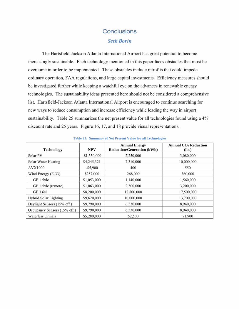
The Hartsfield-Jackson Atlanta International Airport has great potential to become
increasingly sustainable. Each technology mentioned in this paper faces obstacles that must be
overcome in order to be implemented. These obstacles include retrofits that could impede
ordinary operation, FAA regulations, and large capital investments. Efficiency measures should
be investigated further while keeping a watchful eye on the advances in renewable energy
technologies. The sustainability ideas presented here should not be considered a comprehensive
list. Hartsfield-Jackson Atlanta International Airport is encouraged to continue searching for
new ways to reduce consumption and increase efficiency while leading the way in airport
sustainability. Table 25 summarizes the net present value for all technologies found using a 4%
discount rate and 25 years. Figure 16, 17, and 18 provide visual representations.
Table 25: Summary of Net Present Value for all Technologies
Technology NPV Annual Energy
Reduction/Generation (kWh) Annual CO2 Reduction
(lbs) Solar PV -$1,350,000 2,250,000 3,080,000 Solar Water Heating $4,245,321 7,310,000 10,000,000 AVX1000 -$5,900 400 550 Wind Energy (E-33) $257,000 268,000 360,000 GE 1.5xle $1,053,000 1,140,000 1,560,000 GE 1.5xle (remote) $1,063,000 2,300,000 3,200,000 GE 3.6sl $8,200,000 12,800,000 17,500,000 Hybrid Solar Lighting $9,620,000 10,000,000 13,700,000 Daylight Sensors (15% eff.) $9,790,000 6,530,000 8,940,000 Occupancy Sensors (15% eff.) $9,790,000 6,530,000 8,940,000 Waterless Urinals $5,280,000 52,500 71,900

Figure 16: Summary of Net Present Value for all Technologies
Figure 17: Summary of Annual Energy Reduction for all Technologies

Figure 18: Summary of CO2 Emission Reductions for all Technologies

References
AeroVironment, Inc. (2007). Architectural Wind: AVX1000: Building Integrated Wind Turbine. Provided by Terry Civic, Utilities Manager, Massachusetts Port Authority. March 27, 2008.
American Wind Energy Association. (nd). Fair transmission access for wind: a brief discussion
of priority issues. Retrieved on March 20, 2008 from: http://www.awea.org/policy/
documents/transmission.PDF.
Apricus Solar Co. (ASC). (2008). Sizing Solar Hot Water Collectors. Retrieved on March 18,
2008 from http://www.apricus.com/.
Atlanta Gateway Designers (AGD). (2007). Maynard Holbrook Jackson, Jr. International
Terminal (MHJIT) and Parking Structure Schematic Design Report.
Auld and Srinivas. (2006). Aerodynamics for students. Retrieved on March 20, 2008 from:
http://www.aeromech.usyd.edu.au/aero/propeller/index.html.
Bracken, D. (2007, December 26). Triangle isn't sold on waterless urinals. The News & Observer,
Raleigh, NC.
Broehl, J. (2006). California Passes Long-Term Solar Energy Plan(article). Renewable
EnergyAccess.com. Retrieved from: http://www.renewableenergyworld.com/rea/news/
story?id=41631.
City of Atlanta – Department of Aviation.. (February 2007). Airport Fact Sheet - Hartsfield-
Jackson Atlanta International Airport. Retreived on April1, 2008. <http://www.atlanta-
airport.com/Default.asp?url=sublevels/airport_info/gmpage.htm>
City of Atlanta Department of Watershed Management. (2008). Water and sewer rate
information. Retrieved on April 1, 2008 from http://www.atlantawatershed.org/
custsrv/water_and_sewer_rates.htm.
Econews. (2007). San Francisco's Green Power Goal: Solar Panels at San Francisco Airport.
Retrieved from: http://scitizen.com/screens/blogPage/viewBlog/sw_viewBlog.php?
idTheme=14&idContribution=1123.
Enercon GmbH. Enercon Wind Turbines: An Overview. Retrieved on March 20, 2008 from:
http://www.enercon.de/www/en/broschueren.nsf/vwwebAnzeige/15686F537B20CA13C
125719400261D37/$FILE/ENERCON_Product_Overview_Eng.pdf.

Energy Efficiency and Renewable Energy (EERE). (2005). Your Home: Solar Water Heaters.
Retrieved on March 14, 2008 from: http://www.eere.energy.gov/consumer/your_home/
water_heating/index.cfm/mytopic=12850.
General Electric. (2005) 1.5 MW Series Wind Turbine. Retrieved on March 20, 2008 from:
http://www.ge-energy.com/prod_serv/products/wind_turbines/en/downloads/
ge_15_brochure.pdf.
General Electric. (2005). 3.6 MW Offshore Series Wind Turbine. Retrieved on March 20, 2008
from: http://www.gepower.com/prod_serv/products/wind_turbines/en/downloads/
ge_36_brochure_new.pdf.
General Electric. (2008). Retrieved from: http://www.gepower.com/businesses/ge_wind_energy/
en/index.htm.
Georgia Institute of Technology and Southern Company. (2007). Southern Winds: Summary
Project Report 2007. Retrieved on April 21, 2008 from: http://www.energy.gatech.edu/
research/Summary-Southern-Winds.pdf.
Georgia Wind Working Group. (nd). Wind Resource of Georgia, Mean Annual Wind Speed at 90
Meters. Retrieved on March 20, 2008 from: http://www.gawwg.org/Offshore90M
Speed.pdf.
Go Solar California. (2008). Official website. Retrieved from: http://www.gosolarcalifornia.ca.
gov/csi/index.html.
Hafemeister, D. (2007). Physic of Societal Issues: Calculations on National Security,
Environment, and Energy. New York: Springer Science+Business Media, LLC.
Hoffer, S., W. Spitz, E. Loboda, and D. Gee. (January 1998). Economic Analysis of Investment
and Regulatory Decisions – Revised Guide. Federal Aviation Administration.
Hybrid Solar Lighting Gaining Momentum around Nation. (2006, August 15). Retrieved April 1,
2008 from the RenewableEnergyAccess.com website from: renewableenergytoday.net/
rea/news/print ?id=45716.
Lighting Research Institute. (2008). Photosensor tutorial. Retrieved on April 22, 2008 from:
http://www.lrc.rpi.edu/programs/NLPIP/tutorials/photosensors/index.asp.
Lutron. (2008). Ecosystem™. Retrieved on April 24, 2008 from: http://www.lutron.com/
CMS400/page.aspx?mn=411&id=5459#howyousave.

Martin, K. (December 2006). Site Specific Optimization of Rotor/Generator Sizing of Wind
Turbines. Masters Thesis, Georgia Institute of Technology School of Mechanical
Engineering.
Massport takes the wind out of high energy costs Boston Logan to receive 20 building-integrated
wind turbines. (2008, March 5). Retrieved on March 20, 2008 from:
http://www.skycontrol.net/airports/massport-takes-the-wind-out-of-high-energy-costs-
boston-logan-to-receive-20-building-integrated-wind-turbines/.
Meikle, K. (2006). Fresno Yosemite International airport (FYI): Request for proposals: Solar
photovoltaic generating system. City of Fresno-Department of Airports.
Muhs, J. (2000). Oak Ridge National Laboratory. Design and Analysis of Hybrid Solar Lighting
and Full-Spectrum Solar Energy Systems. Oak Ridge, TN: Oak Ridge National
Laboratory.
Muhs, J. (2004, February 14). Up Ahead: Hybrid Lighting. Architectural Lighting Magazine.
Retrieved April 8, 2008 from: http://www.archlighting.com/industry-
news.asp?sectionID=0&articleID=453654.
NASA Langley Atmospheric Science Data Center (NASA). (2008). Surface Meteorology &
Solar Energy Data. Retrieved on March 17, 2008 from: http://eosweb.larc.nasa.gov/.
National Climatic Data Center. (nd). Local Climatological Data Publications. Retrieved on
March 20, 2008 from: http://www7.ncdc.noaa.gov/IPS/LCDPubs?action=directget
publications& wban=13874.
National Renewable Energy Laboratory (NREL). (2007). Learning About Renewables. Retrieved
on March 16, 2008 from: http://www.nrel.gov/learning/re_solar.html.
Parker, S. (2007, June 4). Hybrid Solar Lighting Promises 50% Efficiency. Retrieved on April 1,
2008 from the RenewableEnergyWorld website at: http://www.renewableenergy
world.com/rea/news/story?id=48933.
Port of Oakland. SunEdison. (2007). Port of Oakland and SunEdison Flip the Switch on New
Zero Emission Solar Power System, Oakland International
Response™ daylight: integrated controls by Ledalite. (2007). Retrieved on March 14, 2008 from:
http://www.ledalite.com/download/pdf/Response_Daylight_spec_sheet_r2.pdf.
Rosynsky, P.T. (2006). Port of Oakland wants to build, run solar panel field at airport(article),
http://findarticles.com/p/articles/mi_qn4176/is_20060529/ai_n16433055

San Francisco International Airport. (2007). CASE STUDY 30: Catching the rays at San
Francisco. ENVIRONMENTAL INITIATIVES AROUND THE WORLD. Airport
Council International
Schaeffer, J. (2008). Solar Living Source Book. Hopland: Gaiam Real Goods.
Schuerman, M. (2006, April 2). Urinetown 2006: Green Architects Use Heads of the Future.
Retrieved on March 13, 2008 from the New York Observer website at: http://www.
observer.com/node/52045.
Seifert, G. (2006). Wind radar interference. Retrieved on March 20, 2008 from: http://eere.ener
gy.gov/windandhydro/windpoweringamerica/pdfs/workshops/2006_summit/seifert.pdf.
St. John, J. (2007). Fresno Airport will Plug into Solar Power.
http://www.calpilots.org/html/article.php?sid=1767
St. John, J. (2007). Fresno Airport will Plug into Solar Power. Retrieved from: http://www.cal
pilots.org/html/article.php?sid=1767.
Subtitle C – Conservation and Energy Efficiency Provisions, Energy Policy Act of 2005. (2005).
Retrieved on April 23, 2008 from: http://www.efficientbuildings.org/PDFs/Provision
1331.pdf.
SunEdison. (2008). Official Homepage. Retrieved from: www.sunedision.com.
Sunny forecast for hybrid lighting. (2006, September 13). Environmental Science & Technology
Online - Technology News. Retrieved on April 8, 2008 from: pubs.acs.org/subscribe/
journals/esthag-w/2006/sep/tech/kc_lighting.html
Tharpe, J. (2007, October 29). Airport hoping to flush away less water: Hartsfield-Jackson
looking at ways to conserve during drought. Atlanta Journal-Constitution. Retrieved on
March 13, 2008 from: http://www.ajc.com/metro/content/metro/atlanta/stories/2007/10/
28/airportdrought_1029.html.
Union of Concerned Scientists. (nd). Renewable Energy Tax Credit Extended Again, but Risk of
Boom-Bust Cycle in Wind Industry Continues. Retrieved on April 7, 2008 from:
http://www.ucsusa.org/clean_energy/clean_energy_policies/production-tax-credit-for-
renewable-energy.html.
United States Department of Energy. (2006). Solar Energy Technology Program Muti-Year
Program Plan. Office of Energy Efficiency and Renewable Energy. Retrieved from:
http://www1.eere.energy.gov/solar/pdfs/set_myp_2007-2011_proof_1.pdf.

United States Department of Energy. (2008). Energy Efficiency and Renewable Energy.
Retrieved on March 24, 2008 from: http://www1.eere.energy.gov/solar/photo
voltaics.html.
United States Department of Energy. (April 2007). Hybrid Solar Lighting Illuminate Energy
Savings for Government Facilities. Technology Focus, Section 1: 1-13.
United States Energy Information Agency. (2001). Retrieved on April 23, 2008 from:
http://www.eia.doe.gov/emeu/consumptionbriefs/cbecs/pbawebsite/office/office_howuse
elec.htm.
Urinals of Amsterdam Airport Schiphol. (2008). Retrieved on April 11, 2008 from:
http://www.urinal.net/schiphol/.
Waterless No-Flush™ Urinals. (2008). Retrieved on March 14, 2008 from:
http://www.waterless.com/.
Wilson, Ian. Benefit Assessment of Using Continuous Descent Approaches at Atlanta. 24th
Digital Avionics Systems Conference. October 30, 2005 Wiser, R. and M. Bolinger. (2007). Annual Report on U.S. Wind Power Installation, Cost, and
Performance Trends. United States Department of Energy.

Appendix A: Solar Photovoltaic Systems– Equations & Calculations Equations and Calculations
The price of general electricity at airport in 2011 = 6.0*(1.04^3) = 6.5 cents/kwh
The price of general electricity at airport in 2011~2035 = 6.5* ( (1.04) ^ y )) cents/kwh (Yearly total could be provided upon request).
PV Array Size (Number of panels) = PA / ( PVA x 1.1) = about 7500
where PA is the available space on the roof of the parking structure (137,500 ft²), PVA is the estimated panel area (17 ft²) with the assumption that we need 10 % additional space to provide some space clearance for the panels to avoid interference (18.7 ft² Overall space).
Maximum electricity capacity of PV system = 7500x PVP=1.5MW
Where 7500 is the number of panels of the PV array, and the PVP is the estimated energy production capacity of the panels (200W / panel).
Annual electricity production of the PV system
= Available space*4.5(kwh/m^2/day)*365*efficiency(11%) = 2,250,000 kWh/year
Initial Investment Cost:
The PV panel array cost (PVAC) was calculated using the following equations,
PVAC = Σ [ (PV + BOS + I) / ( (1+ i) ^ y ) ]
Where PV is the 2011 projected commercial PV solar electricity price, BOS is the cost of "balance of system" (BOS) components, I is the installation cost, i is the MARR, and y is the year after the installation is completed denoted as ( i = 1,2,3 …). The PVAC reflects the PV panel array cost in 2011 value.
PVAC = Σ [ (PV + BOS + I) / ( (1+ i) ^ y ) ] = Σ [ ($0.10 + $0.30 + $0.20) / ( (1.04) ^ y ) ]
= 351320.736 + 337808.4 + 324815.7692 + 312322.855 + 300310.4375 + 288760.0361 + 277653.8809 + 266974.8854 + 256706.6206 + 246833.289 + 237339.701 + 228211.25 + 219433.8952 + 210994.13 + 202878.9711 + 195075.9338 + 187573.0132 + 180358.6666 + 173421.7948 + 166751.7258 + 160338.1978 + 154171.3441 + 148241.677 + 142540.074 + 137057.7635
= $ 5.7 million

Total Saving Cost:
With utilization of the new PV system, the airport can save money for paying electricity and get incentives for renewable electricity.
General electricity cost (GEC) is estimated by:
GEC = 6.5 * ( (1+ i) ^ y ))
Where 6.5 is the price of general electricity for Airport (6.5 cents/ kwh), i is the estimated annual energy cost increase (4%), and y is the year after 2011 denoted as ( i = 1,2,3 …).
The total money saved (TSM) per 1 kwh by PV system at jth year is
TSMj = GEC + PTI
where PTI is the production tax incentives (1.9 cents / kwh).
Therefore, total money saved of the jth year is:
Si = 2,250,000kwh/year * TSMj
Finally, we can calculate total money saved in 2011 value for the complete analysis period(2011~2035):
NPV_2011 = Σ Sj * (1+i)^-j
where i is the interest rate.

Appendix B: Solar Hot Water Heating – Equations & Calculations
Equations
Annual hot water use was estimated using the following equation, which assumes 10% of total water consumption is heated water:
AHW = 0.1 x DU x d
where AHW is the annual hot water usage in gallons, DU is the average daily water usage in gallons, and d is the number of days used per year. Energy savings from solar hot water heating is estimated by:
AES = I x d
where AES is the estimated annual energy savings in kWh/m2, and I is the isolation level in kWh/m2/day for Atlanta, GA. See Figure 1 below for insolation data:
Insolation Data For Atlanta, GA (33' 39" N)
0
1
2
3
4
5
6
7
Jan Feb Mar Apr May Jun Jul Aug Sep Oct Nov Dec
Month
Ave
rage
Inso
latio
n (k
Wh/
m2/
day)
Monthly Average Annual Average
Figure 19: 10 Year Average Insolation Data for Atlanta, GA (NASA, 2007)
ASHS is dependent on available space and system area implemented. Monetary savings from solar heating is calculated by:

AMS = AES x EC
where AMS is the annual monetary savings in $/ m2, and EC is the average energy cost per kWh. Total area required to satisfy 100% of the hot water heating needs is computed by:
AR = 0.1 x DU x ECR
where AR is the total area required to meet 100% of daily demand in acres, and ECR is the average energy conversion rate of solar heating in gallons/acre. Annual savings is computed for meeting 100% of daily hot water demand. This is computed by:
TAR = AR x AMS
where TAR is the total annual return in $’s. Lastly, the initial cost can be computed as follows:
IC = AR/CC x SCC
where IC is the initial cost, CC is the collector coverage, assumed to be 32 ft2 and SCC is the solar collector cost. The net present value was calculated using the following formula.
Calculations
Calculations were performed assuming DU = 1 million gallons per day (Interview, 2008), d = 365 days/year, the solar conversion constant ECR = 0.0446 m2/gallon, average isolation level, I = 4. 27 kWh/m2/day, Solar Collector cost = $4,500/unit (ASC, 2008).
AHW = 0.1 x 1,000,000 x 365 = 3.65 x 10⁷ gallons
AES = 4.27 kWh/m2/day x 365 days = 1004 kWh/ m2
AMS = 1004 kWh/m2 x $0.08 = $80.32/m2
AR = 0.1 x 1,000,000 gallons x 0.0446 m2/gallon = 4462.4 m2 = 1.1 acres
TAR = 1.1 acres x 4046.825m2/acre x $80.32/m2 = $358,411 annually
IC = 4462.4 m2/32 ft2/unit x 10.764 ft2/m2 x $4,500/unit = $6,754,679

Appendix C: Wind Energy – Technical Background
Maximum Theoretical Efficiency
Wind-turbines generate electricity by harnessing a wind stream's kinetic energy as it
flows across the turbine’s exposed airfoils. Only a percentage of the total kinetic energy is
actually harvested, since the wind does not stop after the turbine. The air mass flow rate across
the turbine hub can be calculated by:
vAm v& ⋅⋅= ρ
where m& is the mass flow rate, ρ is the air density at hub altitude, A is the area defined by the arc of the turbine blades (subtended area), and vv is the wind velocity. The kinetic energy available from a flowing air mass is found by:
K.E. = 2
21 vm v⋅⋅
where m is the instantaneous mass of air flowing through A.? The theoretical available power
is: 3
212
21 vAvmPMAX
vv& ⋅⋅⋅=⋅= ρ
Wind turbines cannot achieve MAXP since they only modify air flow as it passes through the turbine blades. Due to the kinetic energy extracted by the turbine, the wind slows from its free-stream velocity ( ∞vv ) to its turbine velocity ( tvv ) in the vicinity of the hub region. The velocity is
further reduced to the wake velocity ( wvv ) as additional kinetic energy is removed. The resultant power available can then be found from:
)( 222
1wt vvvP vvv −⋅⋅⋅= ∞ρ
Assuming ∞≈ vvwvv
31 , the maximum kinetic energy obtained by the rotor system is:
P = )( 32
127
16 Av ⋅⋅⋅⋅ ∞vρ
This result, that a maximum 59% of the kinetic energy can be captured, is known as the
“Betz” Limit. As wind velocity decreases near the rotor, a pressure gradient develops with
higher pressure at the downstream region.
The mechanical power delivered to the rotor is from the torque (τ ) imparted by the
passing wind on the blade rotating at a given angular velocity (α ). A reduced angular velocity
increases the available torque, while an increased rotation rate reduces the output torque. This
relationship is significant when evaluating the effect of turbines with multiple rotor blades.

A factor, called the tip-speed ratio, is determined by dividing the tip speed of the blades
( α⋅blader ) by the free-stream velocity ( ∞w ) of the passing wind. Each turbine design has an
optimum tip speed, which is dependent upon the width of each blade and their number. Turbines
with multiple blades have high solidity, where their subtended area has an increased surface area
on which the wind can act. A lower blade count is referred to as a low solidity design, meaning
that the blades will need to rotate at a higher angular velocity to achieve the same efficiency and
power output of a high solidity turbine.
If the tip-speed ratio is too low, less torque is imparted to the blades by the passing air. If
this ratio is too high, some of the air will “bypass” the disc area. Theoretically, a higher blade
count should result in a more efficient turbine rotor. However, high solidity creates interference
between blade elements. Tests have shown 3-bladed designs are the most efficient, followed by
2-bladed and single-bladed versions. Low solidity designs usually operate most efficiently with
electricity-generating turbines, with optimum tip-speed ranging from 6 – 20 (units?).
Turbine Classification
In addition to high- or low- solidity, wind turbines are also classified by their respective
mounting configuration. The most common configuration is the horizontal-axis wind turbine,
also known as the axial-flow turbine, which operates with its rotational axis aligned with the
wind direction. , and a yawing mechanism is required so as to maintain alignment of the axis
into the wind. The performance of this configuration is based upon several factors to include the
number and shape of the blades, aerofoil cross-section, tip-speed ratio, the length of the blade
and it chord, the blade-pitch angle, and the degree of twist preset from the root of the blade to its
tip. Vertical-axis wind turbines, on the other hand, have an axis of rotation that is aligned
vertically and are capable of capturing the wind’s energy despite its direction of origin without
the requirement to reposition the axis. This turbine design is sometimes referred to as a cross-
flow device in that the free-stream wind strikes the blade perpendicular to the axis of rotation.
As the blades rotate, assuming that they rotate sufficiently fast (tip-speed ratio ≥ 3), the angle of
attack of each blade (angle formed between the relative wind and the chord line of the blade)
varies only slightly throughout its full revolution about the axis. With both configurations, the

means by which torque is delivered to the turbine is in accord with the blade-element theory
presented herein.
Blade-Element Theory
This theory is formed under the assumption that the airflow at a given aerofoil cross-
section does not affect the flow at an adjacent cross-section. Therefore, each blade can be
analyzed along its length in determining the net force of the wind applied. Although the blade-
element theory does not account secondary effects such as 3-D flow velocities induced on the
propeller by the shed tip vortex or radial components of flow induced by angular acceleration
due to the rotation of the propeller, a fundamental understanding of these principles is sufficient
for this analysis. Correction factors can be applied that consider these effects accordingly.
The resultant force and torque acting on the turbine blade are dependent upon the flow
geometry of the passing wind stream. The following diagram is provided as a reference for the
ensuing discussion:
Figure 20: Forces and Torques Acting on Turbine Blades (Auld and Srinivas, 2006)
Vectors 210 ,, VandVVvvv
represent the free-stream wind velocity, the relative wind velocity,
and the apparent wind velocity, respectively. The angle of attack (α ) is the angle formed
between the extended chord line of the blade element and the relative wind vector. The lift force
vector acts perpendicular to the relative wind velocity ( 1Vv
), while the drag force acts parallel to
this same vector. The two forces most centric to the generation of electric power in a wind

turbine, however, happen to be those of torque and thrust. As can be seen from the
accompanying diagram, these forces act parallel and perpendicular to the apparent velocity ( 2Vv
),
respectively. Consequently, the developed turbine power is highly dependent upon the rotational
tip-speed of the blades, the importance of which was presented previously.
Intermittency Concerns
As with most renewable energy sources, wind energy is subject to intermittent
availability due to the unpredictability of wind resources. The intermittent nature electric
generation stemming from wind technologies can be modeled by the Rayleigh model distribution
curve, which is closely representative of the hourly distribution of actual wind speeds. Such
modeling strategies can assist renewable energy generators to more accurately predict and
provide a reliable source of energy income to a transmission grid. Nevertheless, wind energy is a
renewable resource, unlike traditional sources such as the finite and nonrenewable coal and
natural gas resources. Additionally, short bursts of high wind speeds can contribute more than
half of the generated energy over a small fraction of a given time period. Consequently, some
form of back-up generation is required when the wind resource cannot meet the periodic
electrical demand. Various storage technologies have been proposed to alleviate some of these
associated problems, but none of these practices have been sufficiently advanced to make wind
an economically viable reality.
Since induction generators are typically employed for wind generation sites, an extensive
array of capacitor banks is employed so as to provide the requisite power factor correction for
interconnectivity with the local power grid. The utility will typically provide the generator with
the required power factor correction needed to maintain a specified tolerance range for fault
reliability. The issue of reliable power output also gives rise to grid management and regulation
policy concerns. A few of these regulatory policy barriers include, but are not limited to,
schedule deviation penalties, interconnection rate pan-caking, and interconnection discrimination.
Interconnection Policy
In order for utilities to provide reliable energy delivery to the end-user, they must schedule
the protracted use of the transmission infrastructure. Traditional power generators will
sometimes deviate from these schedules in response to real-time consumer demand. These

unforeseen circumstances are referred to as “instructed” deviations. However, under certain
circumstances, “uninstructed” deviations might occur due to system malfunctions and/or
operational requirements. This latter case is severely penalized by the utility provider if their
occurrence exceeds an established threshold. For the most part, traditional power generation
schemes can constrain these “uninstructed” events below the predetermined standard. On the
other hand, the intermittent availability of wind power implies that these “uninstructed” incidents
are commanded by nature, and therefore, unfairly discriminate against most renewable resources.
The next regulatory measure that appears to burden the emergence of alternative energy
structures is known as “rate pan-caking,” where a power generator is assessed multiple access
charges when the energy must cross over several “ownership” lines of transmission before it
reaches the end-user. Since wind generation plants must often be sited at remote locations from
the “load center,” these access charges unduly impede the development of the wind industry.
Such rate structures must be eliminated in order to facilitate an economically-viable distribution
of alternative power.
Lastly, interconnection to the utility grid provides yet another obstacle to emerging
generation technologies, primarily driven by utility incentives intended to discourage market
entry by new competitors. Since wind power plants are installed incrementally rather than in
substantial capacity segments, this piece-meal effect exacerbates the associated interconnection
delays. The intermittent nature of wind also requires that the interconnectivity costs, which are
typically based upon peak power output, must be spread across inherently diminished sales of
kilowatt-hours. The end result of these interconnection penalties is that the generator encounters
unnecessary delays and associated costs in delivering their energy to the grid system. The
primary means by which to eliminate this market deterrence is to have requests for
interconnections administered by an independent and objective entity. As can be observed from
the aforementioned hindrances to emerging technologies, it is essential that these transmission
policies be remediated if renewable energy resources are effectively brought to bear in providing
a more diversified energy allocation.

Appendix D: Daylight & Occupancy Sensors – Calculations
The airport consumes an estimated 197.9 million kWh of electricity per year.
Calculations for daylight and occupancy sensors follow.
Airport Building Electricity Consumption = 197.9 million kWh / 2 = 98.93 million kWh
Airport Lighting Electricity Consumption = 0.44 * 98.93 million kWh = 43.53 million kWh
Reduction in Lighting Use = x * 43.53 million kWh where x is the percent reduction
= 0.15 * 43.53 million kWh = 6.53 million kWh
CO2 reductions = Reduction in Lighting Use * 1.37 lbs CO2/kWh
= 6.53 million kWh * 1.37 lbs CO2/kWh = 8.94 million lbs CO2
Net Present Value of Lighting Savings

Appendix E: Waterless Urinals – Equations & Calculations
Equations
Urinal use was estimated using the following equation, which assumes half of the visitors are males:
where EUU is the estimated urinal usage in times, V is the total number of visitors per year, and x is the percentage of urinal use by males. Water savings from waterless urinals is estimated by:
where EWS is the estimated water savings in gallons per year and y is water usage in gallons of current urinals. The cost of BlueSeal® is estimated by the following equation:
The cost of Ecotrap® replacement is estimated by the following equation:
where M is the number of urinals replaced. Water and wastewater costs are calculated by the following equation:
where Cost SavedW is the water and wastewater cost savings from waterless urinal use and Wrate is the rate schedule applicable to the airport. The net present value of cost savings from waterless urinal implementation is calculated by:
where CR is the cost of a regular urinal, CW is the cost of the waterless urinal, t is the cash flow duration, N is the total project time, ra is the inflation rate of water and wastewater rates, rb is the inflation rate of BlueSeal® and EcoTrap® costs, rc is the discount rate, and Ct is the net cash flow at time t.

Calculations
Calculations were performed assuming V = 8.7 million people per year, x = 75% urinal use, and y = 0.5 gallons of water.
= $211,889
