growth curve cognitive diagnosis models for longitudinal
TRANSCRIPT
Growth Curve Cognitive Diagnosis Models for Longitudinal Assessment
by
Seung Yeon Lee
A dissertation submitted in partial satisfaction of the
requirements for the degree of
Doctor of Philosophy
in
Education
in the
Graduate Division
of the
University of California, Berkeley
Committee in charge:
Professor Sophia Rabe-Hesketh, ChairAssistant Professor Zachary Pardos
Professor Nicholas Jewell
Summer 2017

Growth Curve Cognitive Diagnosis Models for Longitudinal Assessment
Copyright 2017by
Seung Yeon Lee
1
Abstract
Growth Curve Cognitive Diagnosis Models for Longitudinal Assessment
by
Seung Yeon Lee
Doctor of Philosophy in Education
University of California, Berkeley
Professor Sophia Rabe-Hesketh, Chair
This dissertation proposes longitudinal growth curve cognitive diagnosis models (GC-CDM) to incorporate learning over time into the cognitive assessment framework. Theapproach was motivated by higher-order latent trait models (de la Torre & Douglas, 2004),which define a higher-order continuous latent trait that affects all the latent skills. Thehigher-order latent trait can be viewed as the more broadly defined general ability; and theskills can be viewed as the specific knowledge arising from the higher-order latent trait. GC-CDMs trace changes in the higher-order latent traits over time by using latent growth curvemodel with respondent-specific random intercept and random slope of time, and simultane-ously trace students’ skill mastery through the CDM measurement model.
GC-CDMs are estimated using marginal maximum likelihood (MML) estimation in Mplus.Relevant issues for estimating GC-CDMs are addressed, e.g., the high-dimensional compu-tation problem, model specification for the relationship between the higher-order latent traitand the multiple skills, and model identification. In simulation studies, we use the DINAmeasurement model, and examine parameter recovery of the GC-DINA model under differingconditions. Particularly, the effects of the design of the Q-matrix, the number of respondentsand the number of time points are discussed. Overall, MML estimation in Mplus shows goodparameter recovery; especially, the average growth, which is the parameter of most interest,is well estimated in all conditions. We also illustrate the application of the GC-DINA modelto real data using two datasets from multi-wave experiments designed to assess the effectsof the Enhanced Anchored Instruction (EAI; Bottge et al., 2003) on mathematics achieve-ment. In addition, the GC-DINA model is compared to the latent transition analysis DINAmodel (LTA-DINA) (Li et al., 2016; Kaya & Leite, 2016) and a longitudinal item responsetheory (IRT) model (Andersen, 1985) using a simulated data. The results suggest that theGC-DINA model and the LTA-DINA model are similar in terms of the predicted skill mas-

2
tery; and the GC-DINA model and the longitudinal IRT model are similar in terms of thepredicted higher-order latent trait.
Keywords: cognitive diagnosis models, higher-order latent trait models, item response mod-els, latent growth curve models, latent transition models, longitudinal assessment, diagnosticclassification models, latent class analysis
i
Contents
Contents i
List of Figures iii
List of Tables v
1 Introduction 1
2 Literature Review: Previous Approaches to Longitudinal Modeling 32.1 Item Response Theory for Measuring Change in Latent Ability . . . . . . . . 32.2 Cognitive Diagnosis Models for Assessing Change in Mastery of Latent Skills 72.3 Dynamic Bayesian Networks for Assessing Change in Knowledge States . . . 10
3 Growth Curve Cognitive Diagnosis Models 143.1 Model . . . . . . . . . . . . . . . . . . . . . . . . . . . . . . . . . . . . . . . 143.2 Estimation . . . . . . . . . . . . . . . . . . . . . . . . . . . . . . . . . . . . . 183.3 Model when the Number of Occasions is Two . . . . . . . . . . . . . . . . . 24
4 Simulation Study 254.1 Simulation Study 1 . . . . . . . . . . . . . . . . . . . . . . . . . . . . . . . . 254.2 Simulation Study 2 . . . . . . . . . . . . . . . . . . . . . . . . . . . . . . . . 42
5 Empirical Study 455.1 Fraction of the Cost (FOC) test data . . . . . . . . . . . . . . . . . . . . . . 455.2 Problem Solving Test (PST) data . . . . . . . . . . . . . . . . . . . . . . . . 51
6 Comparison of Longitudinal Psychometric Models 566.1 Introduction . . . . . . . . . . . . . . . . . . . . . . . . . . . . . . . . . . . . 566.2 Method . . . . . . . . . . . . . . . . . . . . . . . . . . . . . . . . . . . . . . 576.3 Results . . . . . . . . . . . . . . . . . . . . . . . . . . . . . . . . . . . . . . . 57

ii
7 Conclusion 64
A R and Mplus Codes for Chapter 3 66A.1 R code generating data from the HO-DINA with the Rasch model . . . . . . 66A.2 R code generating data from the HO-DINA with the 2PL model . . . . . . . 68A.3 Mplus code of the HO-DINA with the Rasch model . . . . . . . . . . . . . . 69A.4 MODEL command syntax of the Mplus code of the HO-DINA with the 2PL model 82
B R and Mplus Codes for Chapter 4 83B.1 R code for the simulation study for comparison between the simple and com-
plex Q-matrix for the simple DINA model . . . . . . . . . . . . . . . . . . . 83B.2 R code generating six data sets for Model 1 to Model 6 . . . . . . . . . . . . 87B.3 Mplus code for fitting the GC-DINA model for Model 1 to Model 6 . . . . . 90B.4 R code generating data for simulation study 2 . . . . . . . . . . . . . . . . . 116B.5 Mplus code for fitting the GC-DINA in simulation study 2 . . . . . . . . . . 118
C R and Mplus Codes for Chapter 6 141C.1 Mplus code for the LTA-DINA model . . . . . . . . . . . . . . . . . . . . . . 141C.2 Mplus code for the longitudinal Rasch model . . . . . . . . . . . . . . . . . . 141
References 144
iii
List of Figures
2.1 Knowledge tracing models . . . . . . . . . . . . . . . . . . . . . . . . . . . . . . 122.2 Markov decision process framework (Almond, 2007a) . . . . . . . . . . . . . . . 132.3 Simple dynamic Bayesian network with two time points (Culbertson, 2016) . . . 13
3.1 Growth curve cognitive diagnosis model (subscript j not shown) . . . . . . . . . 173.2 Scatter plots of item parameter estimates : (1) Mplus Rasch/1PL estimates vs.
generating values and (2) Mplus Rasch/1PL vs. GDINA 1PL. . . . . . . . . . . 223.3 Scatter plots of item parameter estimates : (1) Mplus 2PL estimates vs. gener-
ating values and (2) Mplus 2PL vs. GDINA 2PL. . . . . . . . . . . . . . . . . . 23
4.1 Scatter plots of GC-DINA item parameter estimates vs. generating values forModel 1 and Model 2. . . . . . . . . . . . . . . . . . . . . . . . . . . . . . . . . 39
4.2 Scatter plots of GC-DINA item parameter estimates vs. generating values forModel 3 and Model 4. . . . . . . . . . . . . . . . . . . . . . . . . . . . . . . . . 40
4.3 Scatter plots of GC-DINA item parameter estimates vs. generating values forModel 5 and Model 6. . . . . . . . . . . . . . . . . . . . . . . . . . . . . . . . . 41
4.4 Scatter plots of GC-DINA item parameter estimates vs. generating values forsimulation study 2. . . . . . . . . . . . . . . . . . . . . . . . . . . . . . . . . . . 43
4.5 Scatter plots of predicted higher-order latent traits from the GC-DINA modelvs. generating values for simulation study 2. The estimated correlation, r, is inparenthesis. . . . . . . . . . . . . . . . . . . . . . . . . . . . . . . . . . . . . . . 44
5.1 Predicted growth trajectories in the higher-order latent trait across four timepoints for the FOC data. . . . . . . . . . . . . . . . . . . . . . . . . . . . . . . . 48
5.2 Scatter plots of GC-DINA item parameter estimates vs. LTA-DINA item param-eter estimates reported in Li et al. (2016) for the FOC data. . . . . . . . . . . . 49
5.3 Scatter plots of GC-DINA item parameter estimates vs. generating values for thesimulated data using parameters recovered from the FOC data. . . . . . . . . . 51
iv
5.4 Scatter plots of GC-DINA item parameter estimates vs. generating values for thesimulated data using parameters recovered from the PST data. . . . . . . . . . . 55
6.1 Scatter plots of predicted higher-order latent traits vs. generating values: (1)GC-DINA estimates vs. generating values and (2) longitudinal Rasch estimatesvs. generating values. The estimated correlation, r, is in parenthesis. . . . . . . 62
6.2 Scatter plots of predicted higher-order latent traits: GC-DINA estimates vs. lon-gitudinal Rasch estimates. The estimated correlation, r, is in parenthesis. . . . . 63
v
List of Tables
3.1 Q-matrix of 20 items and 4 skills for the HO-DINA model simulation study. . . 203.2 Estimated parameter values from Mplus and GDINA R package. . . . . . . . . . 21
4.1 Simple Q-matrix of 20 items and 4 skills for the simulation study. . . . . . . . . 274.2 Complex Q-matrix of 20 items and 4 skills for the simulation study. . . . . . . . 274.3 Classification accuracy with the simple and complex Q-matrices for the simple
DINA model. . . . . . . . . . . . . . . . . . . . . . . . . . . . . . . . . . . . . . 274.4 Parameter estimates and standard errors (in parentheses) for Model 1 and Model 2 314.5 Parameter estimates and standard errors (in parentheses) for Model 3 and Model 4 324.6 Parameter estimates and standard errors (in parentheses) for Model 5 and Model 6 334.7 Square root of relative efficiencies for β: the simple Q-matrix vs. the complex
Q-matrix. . . . . . . . . . . . . . . . . . . . . . . . . . . . . . . . . . . . . . . . 344.8 Parameter estimates and standard errors (in parentheses) for Model 1 and Model 3 364.9 Parameter estimates and standard errors (in parentheses) for Model 3 and Model 5 374.10 Generating values and GC-DINA estimates for simulation study 2. . . . . . . . . 43
5.1 Q-matrix for Fraction of Cost (FOC) test. . . . . . . . . . . . . . . . . . . . . . 475.2 Estimated GC-DINA model parameters for the FOC data. . . . . . . . . . . . . 485.3 Proportion of students predicted to have mastered each skill at each occasion for
the FOC data (LTA results from Li et al. (2016)). . . . . . . . . . . . . . . . . . 495.4 GC-DINA parameter estimates and standard errors for the simulated data using
parameters recovered from the FOC data. . . . . . . . . . . . . . . . . . . . . . 505.5 Q-matrix for Problem Solving Test (PST). . . . . . . . . . . . . . . . . . . . . . 525.6 GC-DINA parameter estimates and standard errors for the PST data. . . . . . . 535.7 GC-DINA item parameter estimates and standard errors for the PST data. . . . 545.8 Proportion of students predicted to have mastered each skill at each occasion for
the PST data. . . . . . . . . . . . . . . . . . . . . . . . . . . . . . . . . . . . . . 545.9 GC-DINA parameter estimates and standard errors for the simulated data using
parameters recovered from the PST data. . . . . . . . . . . . . . . . . . . . . . . 55
vi
6.1 Parameter estimates for the GC-DINA model and the longitudinal Rasch model. 586.2 Higher-order structural parameter estimates for the GC-DINA model. . . . . . . 596.3 Parameter estimates for the LTA-DINA model. . . . . . . . . . . . . . . . . . . 596.4 Item parameter estimates for the GC-DINA model, the LTA-DINA model, and
the longitudinal Rasch model. . . . . . . . . . . . . . . . . . . . . . . . . . . . . 596.5 Model fit information of the GC-DINA model, the LTA-DINA model, and the
longitudinal Rasch model. . . . . . . . . . . . . . . . . . . . . . . . . . . . . . . 606.6 Proportion of correctly classified skills (PCS) and last element of the proportion
of correctly classified skill profile vectors (PCV) for the GC-DINA model and theLTA-DINA model. . . . . . . . . . . . . . . . . . . . . . . . . . . . . . . . . . . 60
6.7 Model-implied probability of having each skill at each time point for the GC-DINA model and the LTA-DINA model. . . . . . . . . . . . . . . . . . . . . . . 61

vii
Acknowledgments
First and foremost, I would like to express the deepest gratitude to my advisor ProfessorSophia Rabe-Hesketh. This work would not have been possible without her unwaveringsupport and intellectual guidance that she has provided to me over the last five years. Shehas not only shown me the route to scholarly curiosity, but also served as a mentor, aguide, and a true friend as I was about to succumb, when faced with numerous hurdlesthroughout the process. I also would like to thank the professors who served as members ofmy dissertation committee. I thank Professor Zachary Pardos, because without him, I wouldnot have had a chance to get introduced to the exciting world of educational data mining. Ithank Professor Nicholas Jewell, for his insightful and indispensable comments on my workfrom the very first draft to the very last one. I thank Professor Mark Wilson, as he was theone who brought me in the realm of educational measurement.
I was truly fortunate to meet great mentors, colleagues and friends along the way. I sin-cerely appreciate the learning experience UCSF Department of Psychiatry provided, includ-ing Professor Kaja LeWinn, Katrina Roundfield and Ellen Kersten. I am deeply indebted toProfessors Taeyoung Park and Hakbae Lee at Yonsei University for their support throughoutmy academic journey. I am grateful to all my friends I met in Berkeley, and special thanksto QME folks.
Finally, my sincere and greatest appreciation goes to my family who provided uncondi-tional love and support throughout my life. This dissertation is dedicated to them.
1
Chapter 1
Introduction
In educational measurement, psychometric models have been used to measure students’ la-tent characteristics such as knowledge or aptitude. One well-known class of psychometricmodels are item response theory (IRT) models. IRT models define students’ ability as con-tinuous latent variables and have been used to order students on a continuum. Recently, cog-nitive diagnosis models (CDM), alternatively called diagnostic classification models (DCM;e.g., Rupp et al., 2010), have received increasing attention. CDMs define the target profi-ciency as a set of multiple skills specified at a fine grain size. By examining students’ masteryof these skills, the model provides diagnostic information for instruction and learning, i.e.,students’ strengths and weaknesses in the domain.
Most CDMs treat responses as if they were from a single time point and do not accountfor change in knowledge proficiency across time. Students’ skill knowledge, however, changesover time as they learn and it is important to know their learning trajectories. For example,students take periodic tests to prepare for high stakes exams in schools or students interactwith intelligent tutors on a daily basis to prepare for an end of unit exam. In addition,pre-post tests can be administrated to evaluate educational treatments. By understandingstudents’ learning over time, educators can monitor students’ progress toward learning goalsand decide what to adjust to achieve better learning; and students themselves can also beinformed on what they can and cannot and what they need to focus on next to reach theirgoals. However, while there is an extensive literature on IRT-based longitudinal models,little work has been done on extending CDMs for longitudinal settings.
In this dissertation, I propose a longitudinal CDM, “growth curve cognitive diagnosismodel” (GC-CDM). GC-CDMs were motivated by higher-order latent trait models (de laTorre & Douglas, 2004), which define a higher-order continuous latent trait that affects allthe latent skills. The higher-order latent trait can be viewed as the more broadly definedgeneral ability associated with the fine grained skills. GC-CDMs trace changes in the higher-order latent traits over time by using latent growth modeling for the higher order traits and
CHAPTER 1. INTRODUCTION 2
simultaneously trace students’ skill mastery through the CDM measurement model.The outline of this dissertation is as follows. Chapter 2 reviews commonly used psycho-
metric models (i.e., item response theory models, cognitive diagnosis models and dynamicBayesian networks) and their extension for analysis of longitudinal data. Chapter 3 in-troduces our proposed method, GC-CDMs. The details of the modeling framework andthe estimation method are discussed. In Chapter 4, two simulation studies are discussed.We particularly examine parameter recovery for the GC-CDM under various conditions.Chapter 5 discusses application of GC-CDMs to two datasets from the Enhanced AnchoredInstruction (EAI; Bottge et al., 2003) project. In Chapter 6, different longitudinal psycho-metric models are compared using a simulated data set from the GC-CDM. We end with aconclusion in Chapter 7.
3
Chapter 2
Literature Review: PreviousApproaches to Longitudinal Modeling
In educational assessment, different types of psychometric models exist and there have beenincreasing efforts to extend them for the analysis of longitudinal data. This chapter re-views commonly used psychometric models and discusses existing longitudinal modeling ap-proaches in each framework. In particular, item response theory models, cognitive diagnosismodels and Bayesian networks will be discussed.
2.1 Item Response Theory for Measuring Change in
Latent Ability
Item Response Theory (IRT) Models
Item response theory (IRT) is used to develop, score and analyze assessments that measurerespondents’ latent characteristics. In education, IRT has been widely used in large-scaleassessments measuring students’ ability. The main idea of IRT is the item response function(IRF), which specifies the probability of a given response as a function of the student’s trueability.
The simplest IRT model for binary responses (Y = 0 if the question or item has beenanswered incorrectly and Y = 1 if it has been answered correctly) is the one-parameterlogistic (1PL) model with an item difficulty parameter for each item, most commonly knownas the Rasch (Rasch, 1961) model. Under the Rasch model, the probability that person jwith latent ability θj gives a correct response (Yij = 1) to item i with difficulty βi is
P(Yij = 1|θj) =exp(θj − βi)
1 + exp(θj − βi). (2.1)
CHAPTER 2. LITERATURE REVIEW: PREVIOUS APPROACHES TOLONGITUDINAL MODELING 4
The model with two item parameters, item difficulty and discrimination, is called the two-parameter logistic (2PL) model (Birnbaum, 1968) and is defined as
P(Yij = 1|θj) =exp{αi(θj − βi)}
1 + exp{αi(θj − βi)}, (2.2)
where αi is the discrimination and βi is the difficulty of item i. The discrimination parametercharacterizes how well the item differentiates among persons who are at different abilitylevels.
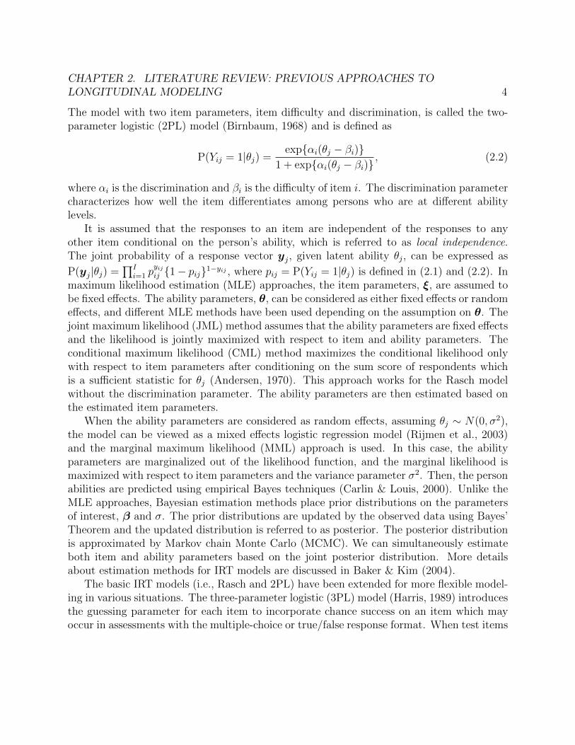
It is assumed that the responses to an item are independent of the responses to anyother item conditional on the person’s ability, which is referred to as local independence.The joint probability of a response vector yj, given latent ability θj, can be expressed as
P(yj|θj) =∏I
i=1 pyijij {1− pij}1−yij , where pij = P(Yij = 1|θj) is defined in (2.1) and (2.2). In
maximum likelihood estimation (MLE) approaches, the item parameters, ξ, are assumed tobe fixed effects. The ability parameters, θ, can be considered as either fixed effects or randomeffects, and different MLE methods have been used depending on the assumption on θ. Thejoint maximum likelihood (JML) method assumes that the ability parameters are fixed effectsand the likelihood is jointly maximized with respect to item and ability parameters. Theconditional maximum likelihood (CML) method maximizes the conditional likelihood onlywith respect to item parameters after conditioning on the sum score of respondents whichis a sufficient statistic for θj (Andersen, 1970). This approach works for the Rasch modelwithout the discrimination parameter. The ability parameters are then estimated based onthe estimated item parameters.
When the ability parameters are considered as random effects, assuming θj ∼ N(0, σ2),the model can be viewed as a mixed effects logistic regression model (Rijmen et al., 2003)and the marginal maximum likelihood (MML) approach is used. In this case, the abilityparameters are marginalized out of the likelihood function, and the marginal likelihood ismaximized with respect to item parameters and the variance parameter σ2. Then, the personabilities are predicted using empirical Bayes techniques (Carlin & Louis, 2000). Unlike theMLE approaches, Bayesian estimation methods place prior distributions on the parametersof interest, β and σ. The prior distributions are updated by the observed data using Bayes’Theorem and the updated distribution is referred to as posterior. The posterior distributionis approximated by Markov chain Monte Carlo (MCMC). We can simultaneously estimateboth item and ability parameters based on the joint posterior distribution. More detailsabout estimation methods for IRT models are discussed in Baker & Kim (2004).
The basic IRT models (i.e., Rasch and 2PL) have been extended for more flexible model-ing in various situations. The three-parameter logistic (3PL) model (Harris, 1989) introducesthe guessing parameter for each item to incorporate chance success on an item which mayoccur in assessments with the multiple-choice or true/false response format. When test items
CHAPTER 2. LITERATURE REVIEW: PREVIOUS APPROACHES TOLONGITUDINAL MODELING 5
are associated with more than one latent trait such as in personality assessments, multidi-mensional IRT models (Van Der Linden & Hambleton, 1997) have been applied. ExplanatoryIRT incorporates explanatory variables (e.g., item covariates, person covariates) to take intoaccount different characteristics among items and persons, such as why some items are moredifficult than others and why some students have higher abilities than others (De Boeck &Wilson, 2004). For the situation in which the sample of respondents consists of several latentsub-populations that are qualitatively different but an IRT measurement model holds withineach subgroup, mixture IRT models (Rost, 1990)—a combination of IRT and latent classanalysis (LCA)—has been developed.
IRT-based Longitudinal Models
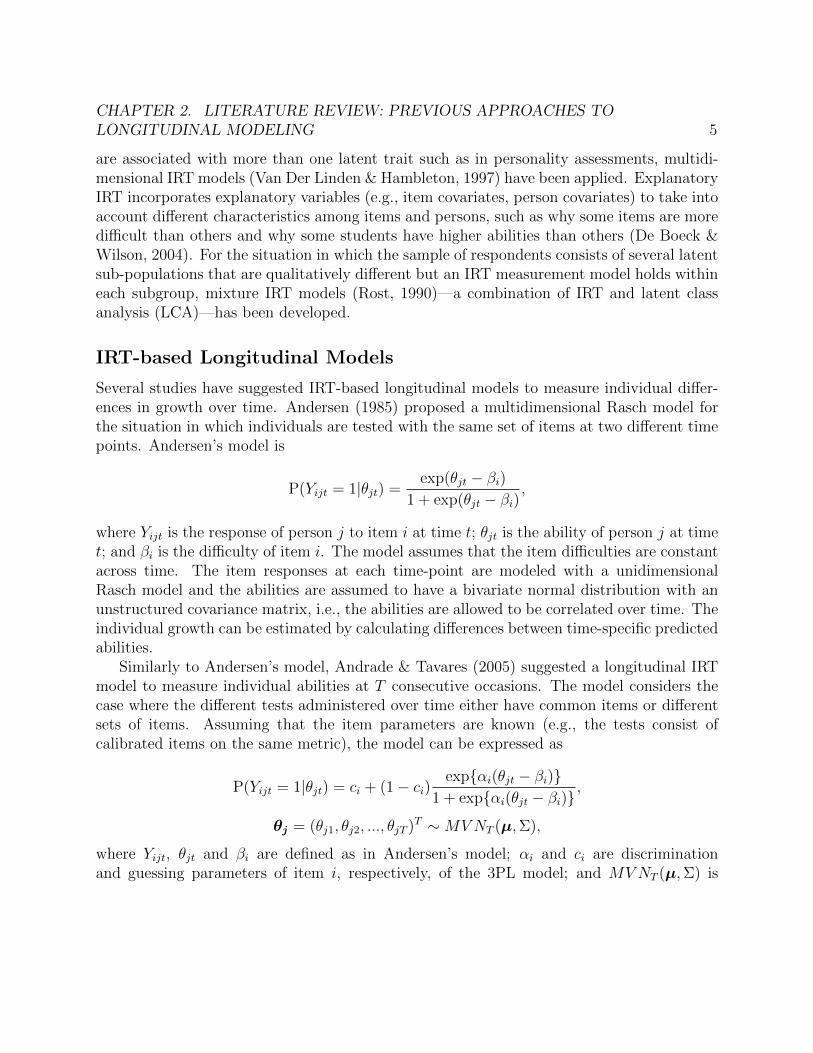
Several studies have suggested IRT-based longitudinal models to measure individual differ-ences in growth over time. Andersen (1985) proposed a multidimensional Rasch model forthe situation in which individuals are tested with the same set of items at two different timepoints. Andersen’s model is
P(Yijt = 1|θjt) =exp(θjt − βi)
1 + exp(θjt − βi),
where Yijt is the response of person j to item i at time t; θjt is the ability of person j at timet; and βi is the difficulty of item i. The model assumes that the item difficulties are constantacross time. The item responses at each time-point are modeled with a unidimensionalRasch model and the abilities are assumed to have a bivariate normal distribution with anunstructured covariance matrix, i.e., the abilities are allowed to be correlated over time. Theindividual growth can be estimated by calculating differences between time-specific predictedabilities.
Similarly to Andersen’s model, Andrade & Tavares (2005) suggested a longitudinal IRTmodel to measure individual abilities at T consecutive occasions. The model considers thecase where the different tests administered over time either have common items or differentsets of items. Assuming that the item parameters are known (e.g., the tests consist ofcalibrated items on the same metric), the model can be expressed as
P(Yijt = 1|θjt) = ci + (1− ci)exp{αi(θjt − βi)}
1 + exp{αi(θjt − βi)},
θj = (θj1, θj2, ..., θjT )T ∼MVNT (µ,Σ),
where Yijt, θjt and βi are defined as in Andersen’s model; αi and ci are discriminationand guessing parameters of item i, respectively, of the 3PL model; and MVNT (µ,Σ) is
CHAPTER 2. LITERATURE REVIEW: PREVIOUS APPROACHES TOLONGITUDINAL MODELING 6
the T -dimensional multivariate normal distribution with mean vector µ and unstructuredcovariance matrix Σ.
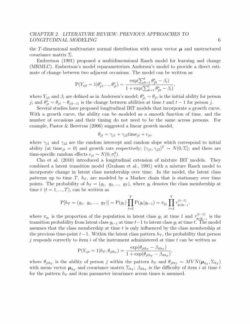
Embretson (1991) proposed a multidimensional Rasch model for learning and change(MRMLC). Embretson’s model reparameterizes Andersen’s model to provide a direct esti-mate of change between two adjacent occasions. The model can be written as
P(Yijt = 1|θ∗j1, ..., θ∗jt) =exp(
∑tk=1 θ
∗jk − βi)
1 + exp(∑t
k=1 θ∗jk − βi)
,
where Yijt and βi are defined as in Andersen’s model; θ∗j1 = θj1 is the initial ability for personj; and θ∗jt = θjt − θj(t−1) is the change between abilities at time t and t− 1 for person j.
Several studies have proposed longitudinal IRT models that incorporate a growth curve.With a growth curve, the ability can be modeled as a smooth function of time, and thenumber of occasions and their timing do not need to be the same across persons. Forexample, Pastor & Beretvas (2006) suggested a linear growth model,
θjt = γj1 + γj2timejt + εjt,
where γj1 and γj2 are the random intercept and random slope which correspond to initialability (at timejt = 0) and growth rate respectively; (γj1, γj2)
T ∼ N(0,Σ); and there aretime-specific random effects εjt ∼ N(0, σ2
ε ).Cho et al. (2010) introduced a longitudinal extension of mixture IRT models. They
combined a latent transition model (Graham et al., 1991) with a mixture Rasch model toincorporate change in latent class membership over time. In the model, the latent classpatterns up to time T , hT , are modeled by a Markov chain that is stationary over timepoints. The probability of hT = (g1, g2, ..., gT ), where gt denotes the class membership attime t (t = 1, ..., T ), can be written as
P[hT = (g1, g2, ..., gT )] = P(g1)T∏t=2
P(gt|gt−1) = πg1
T∏t=2
τ(t−1)gt|gt−1
,
where πg1 is the proportion of the population in latent class g1 at time 1 and τ(t−1)gt|gt−1
is thetransition probability from latent class gt−1 at time t−1 to latent class gt at time t. The modelassumes that the class membership at time t is only influenced by the class membership atthe previous time-point t−1. Within the latent class pattern hT , the probability that personj responds correctly to item i of the instrument administered at time t can be written as
P(Yijt = 1|hT , θjthT ) =exp(θjthT − βithT )
1 + exp(θjthT − βithT ),
where θjthT is the ability of person j within the pattern hT and θjthT ∼ MVN(µhT ,ΣhT )with mean vector µhT and covariance matrix ΣhT ; βithT is the difficulty of item i at time tfor the pattern hT and item parameter invariance across times is assumed.
CHAPTER 2. LITERATURE REVIEW: PREVIOUS APPROACHES TOLONGITUDINAL MODELING 7
2.2 Cognitive Diagnosis Models for Assessing Change
in Mastery of Latent Skills
Cognitive Diagnosis Models
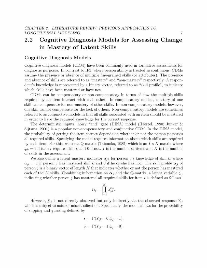
Cognitive diagnosis models (CDM) have been commonly used in formative assessments fordiagnostic purposes. In contrast to IRT where person ability is treated as continuous, CDMsassume the presence or absence of multiple fine-grained skills (or attributes). The presenceand absence of skills are referred to as “mastery” and “non-mastery” respectively. A respon-dent’s knowledge is represented by a binary vector, referred to as “skill profile”, to indicatewhich skills have been mastered or have not.
CDMs can be compensatory or non-compensatory in terms of how the multiple skillsrequired by an item interact with each other. In compensatory models, mastery of oneskill can compensate for non-mastery of other skills. In non-compensatory models, however,one skill cannot compensate for the lack of others. Non-compensatory models are sometimesreferred to as conjunctive models in that all skills associated with an item should be masteredin order to have the required knowledge for the correct response.
The deterministic inputs, noisy “and” gate (DINA) model (Haertel, 1990; Junker &Sijtsma, 2001) is a popular non-compensatory and conjunctive CDM. In the DINA model,the probability of getting the item correct depends on whether or not the person possessesall required skills. Specifying the model requires information about which skills are requiredby each item. For this, we use a Q-matrix (Tatsuoka, 1985) which is an I ×K matrix whereqik = 1 if item i requires skill k and 0 if not. I is the number of items and K is the numberof skills in the assessment.
We also define a latent mastery indicator αjk for person j’s knowledge of skill k, whereαjk = 1 if person j has mastered skill k and 0 if he or she has not. The skill profile αj ofperson j is a binary vector of length K that indicates whether or not the person has masteredeach of the K skills. Combining information on αj and the Q-matrix, a latent variable ξijindicating whether person j has mastered all required skills for item i is defined as follows
ξij =K∏k=1
αqikjk .
However, ξij is not directly observed but only indirectly via the observed response Yijwhich is subject to noise or misclassification. Specifically, the model allows for the probabilityof slipping and guessing defined by
si = P(Yij = 0|ξij = 1),
gi = P(Yij = 1|ξij = 0).

CHAPTER 2. LITERATURE REVIEW: PREVIOUS APPROACHES TOLONGITUDINAL MODELING 8
The slipping parameter (si) is the probability that person j responds incorrectly to item ieven if he or she has mastered all required skills (ξij = 1). The guessing parameter (gi) isthe probability that person j responds correctly to item i even if he or she has not masteredall the required skills (ξij = 0).
The probability of a correct response of person j for item i, πij, is represented by theDINA model as follows:
πij = P(Yij = 1|αj) = (1− si)ξijg1−ξiji . (2.3)
The deterministic inputs, noisy “or” gate (DINO) model (Templin & Henson, 2006) isthe compensatory analog to the DINA model. DINO assumes that a respondent has enoughknowledge required by an item if he or she has mastered at least one of the associated skills.The latent variable ξij in DINO is defined by
ξij = 1−K∏k=1
(1− αjk)qik .
Just as in the DINA model, slipping and guessing processes are modeled at the item leveland the probability of a correct response to an item is modeled as in (2.3).
The DINA or DINO models determine the probability of item responses, Y , given the skillmastery status, α, which corresponds to the measurement part of CDMs. After specifyingthe measurement part of the model, we need to consider the probability distribution ofα = (α1, α2, ..., αK), which is the structural part of the model. Several different types ofstructural models have been discussed for the joint probability distribution of skill masteryacross different skills (Maris, 1999; Rupp et al., 2010). The simplest structural model is theindependence model, which assumes the skill mastery indicators are independent of eachother: P(α1, ..., αK) =
∏Kk=1 P(αk). However, the independence assumption among skills
are not realistic in practice. Other structural models are unstructured, log-linear (Maris,1999; Xu & Davier, 2008), unstructured tetrachoric (Hartz, 2002), and structured tetrachoricmodels. One type of the structured tetrachoric model is the higher-order latent trait modelby de la Torre (2009), which assumes that the skill mastery indicators are conditionallyindependent given the higher-order latent trait. More details of the higher-order latent traitmodel will be discussed in Section 3.1.
In likelihood-based approaches, the item parameters (i.e., guessing and slipping) are oftenestimated by marginal maximum likelihood. In the latent class modeling framework, eachskill profile can be viewed as a latent class and the marginalized likelihood of the data can beexpressed as L(y) =
∏Jj=1
∑Cc=1 νc
∏Ii=1 P(Yij = yij|αc), where αc is the attribute pattern
of latent class c and νc is the probability of membership in latent class c. The likelihood canbe maximized using an EM algorithm. Details of the algorithm for estimating parameters
CHAPTER 2. LITERATURE REVIEW: PREVIOUS APPROACHES TOLONGITUDINAL MODELING 9
of the DINA model are discussed in de la Torre (2009). After the item parameters areestimated, posterior skill mastery probabilities for each person and skill can be obtained byempirical Bayes, and the skill profiles are then predicted by rounding these probabilities to0/1 (i.e., choosing the mastery status with the greater posterior probability). In Bayesianapproaches, we assign prior distributions to the guessing and slipping parameters and bothitem parameters and skill profiles are simultaneously estimated via MCMC.
A number of alternative types of CDMs have been proposed. The noisy input, deter-ministic “And” gate (NIDA) model (Maris, 1999) is an extension of the DINA model butspecifies the slipping and guessing parameters at the skill level. The reparameterized unifiedmodel (RUM) (Hartz, 2002; Roussos et al., 2007) is a generalization of the NIDA and DINAmodels, allowing different slipping and guessing parameters at both the item and skill level.Also, different general modeling frameworks have been suggested, e.g., general diagnosticmodel (GDM) (Davier, 2005), log-linear CDM (LCDM) (Henson et al., 2009) and gener-alized DINA (G-DINA) (de la Torre, 2011). Rupp et al. (2010) provides a comprehensivediscussion of the theory and application of CDMs.
Latent Transition Analysis Cognitive Diagnosis Models
Although CDMs have recently received increasing attention in educational measurement,most CDMs are static models and there has been little previous work on longitudinal cogni-tive diagnosis modeling.
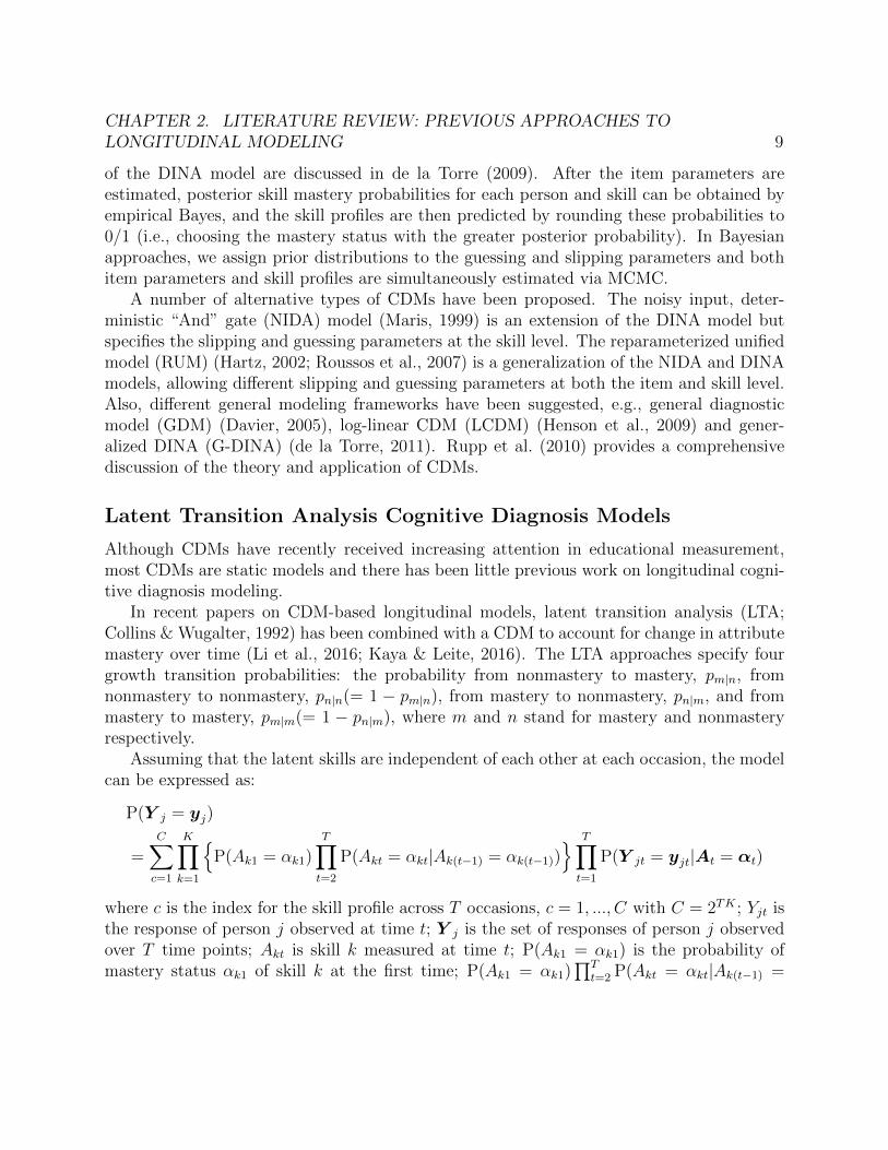
In recent papers on CDM-based longitudinal models, latent transition analysis (LTA;Collins & Wugalter, 1992) has been combined with a CDM to account for change in attributemastery over time (Li et al., 2016; Kaya & Leite, 2016). The LTA approaches specify fourgrowth transition probabilities: the probability from nonmastery to mastery, pm|n, fromnonmastery to nonmastery, pn|n(= 1 − pm|n), from mastery to nonmastery, pn|m, and frommastery to mastery, pm|m(= 1 − pn|m), where m and n stand for mastery and nonmasteryrespectively.
Assuming that the latent skills are independent of each other at each occasion, the modelcan be expressed as:
P(Y j = yj)
=C∑c=1
K∏k=1
{P(Ak1 = αk1)
T∏t=2
P(Akt = αkt|Ak(t−1) = αk(t−1))} T∏t=1
P(Y jt = yjt|At = αt)
where c is the index for the skill profile across T occasions, c = 1, ..., C with C = 2TK ; Yjt isthe response of person j observed at time t; Y j is the set of responses of person j observedover T time points; Akt is skill k measured at time t; P(Ak1 = αk1) is the probability ofmastery status αk1 of skill k at the first time; P(Ak1 = αk1)
∏Tt=2 P(Akt = αkt|Ak(t−1) =
CHAPTER 2. LITERATURE REVIEW: PREVIOUS APPROACHES TOLONGITUDINAL MODELING 10
αk(t−1)) indicates the probability of a sequence of skill mastery indicators for skill k acrossoccasions; and the measurement model P(Y jt = yjt|At = αt) is either the DINA or DINOmodel. The latent transition analysis DINA (LTA-DINA) model assumes that the itemparameters (guessing and slipping) are constant over time, while the skill knowledge stateis allowed to change over time. In addition, transition probabilities P(Akt = αkt|Ak(t−1) =αk(t−1)) are allowed to differ for each skill and are sometimes constrained to be constant overtime.
2.3 Dynamic Bayesian Networks for Assessing
Change in Knowledge States
Bayesian Networks
Bayesian networks (BNs) have been extensively used as student models for intelligent tu-toring systems (ITS; for examples, Bunt & Conati, 2002; Zapata-Rivera & Greer, 2004;Koedinger & Aleven, 2007), and they also have been successfully applied for cognitivelydiagnostic assessments (R. J. Mislevy, 1995; R. Mislevy et al., 1999; Levy & Mislevy, 2004;Sinharay & Almond, 2007). A BN consists of a directed acyclic graph (DAG) and a proba-bility distribution. In the graph, nodes represent random variables and edges between nodesrepresent probabilistic dependencies among them. For the directed edge from node A tonode B, we say that A is a parent of B and B is a child of A. The set of all parents of nodeC, as well as the parents of these parents, etc., are referred to as ancestors of C, and theset of all children of node C including the children of children are called descendants of C.Each node in a BN is conditionally independent of all its non-descendants given the stateof that node’s parents. By the general multiplication rule, the joint probability distributionover all the variables in a BN factorizes into a series of conditional probability distributions.This property provides a convenient way to define the joint distribution compactly by onlyspecifying the conditional probability distribution for every node (Heckerman, 1998; Pearl,1988).
One of the powerful features of BNs is that they can be used for probabilistic inferenceabout unobserved variables through the complete structure of the variables and their rela-tionships. For example, when the leaves (nodes with no children) are observed, the priorbelief on their roots (nodes with no parents) can be updated based on the observed evi-dence by applying Bayes Theorem. There are two kinds of inference algorithms: exact andapproximate. The most common inference methods are variable elimination and a junc-tion tree algorithm for exact inference, and importance sampling and MCMC simulation forapproximate inference.

CHAPTER 2. LITERATURE REVIEW: PREVIOUS APPROACHES TOLONGITUDINAL MODELING 11
When BNs are applied to educational measurement, hidden nodes usually represent dis-crete proficiency levels, and leaves generally represent observed responses to items. Specif-ically, for an assessment designed to measure latent knowledge on multiple skills, BNs canbe used as a CDM approach. Conjunctive or disjunctive CDMs are available in the BNframework using Noisy-OR and Noisy-AND models. The edges from hidden nodes to ob-served nodes correspond to the elements of the Q-matrix. More details about application ofBNs for CDMs are discussed in Almond et al. (2015). One of BNs’ benefits over traditionalCDMs is that BNs can easily incorporate associations between skills into the model by edgesconnecting hidden nodes, which can improve measurement precision.
Dynamic Bayesian Networks in Assessment for Learning Systems
Dynamic Bayesian networks (DBNs) (Dean & Kanazawa, 1989) have been widely used tomodel student learning in ITS. Changes over time can be modeled by two pieces: (1) a singletime-slice model for the initial state of the system and (2) a two-time-slice model for thetransition from one-time slice to the next. By a Markov property, it is assumed that theknowledge state in any time slice is independent of the past history given the previous timeslice. Almond et al. (2015) discusses two ways to model the transition from one state tothe next in learning systems: mathematical learning models and Markov decision process(MDP).
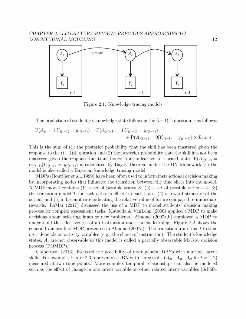
The basic idea of mathematical learning models is that a student has mastered or notmastered a certain knowledge at time t, responds to a practice question, and the mas-tery state at time t + 1 depends on the previous mastery state. A popular example is theknowledge tracing (KT) model introduced by Corbett & Anderson (1994). The KT modelmonitors a student’s proficiency on a single knowledge component during practice, and thesystem provides proper guidance needed for the student and determines when the studenthas reached the mastery. Figure 2.1 presents the basic form of KT models. At is a student’slatent knowledge for a particular skill at time t and Yt is the student’s response to a questionat time t. A circle represents a latent variable and a rectangle represents an observablevariable.
A KT model uses four parameters: Prior, Learn, Guess and Slip. The Prior is P(A1 = 1),which is the initial probability that students know the skill a priori. Learn is the probabil-ity that students’ knowledge state will transition from unlearned (non-mastery) to learned(mastery), P(At = 1|At−1 = 0), after interacting with each question. It is assumed that itis impossible to lose a skill, P(At = 0|At−1 = 1) = 0. Guess is the probability that studentsget a correct answer by guessing when they do not know the skill, and Slip is the probabilitythat students respond incorrectly to an item by slipping although they know the skill.
CHAPTER 2. LITERATURE REVIEW: PREVIOUS APPROACHES TOLONGITUDINAL MODELING 12
A1
Y1
t=1
A2
Y2
t=2
A3
Y3
t=3
Growth
Figure 2.1: Knowledge tracing models
The prediction of student j’s knowledge state following the (t−1)th question is as follows:
P(Ajt = 1|Yj(t−1) = yj(t−1)) = P(Aj(t−1) = 1|Yj(t−1) = yj(t−1))
+ P(Aj(t−1) = 0|Yj(t−1) = yj(t−1))× Learn
This is the sum of (1) the posterior probability that the skill has been mastered given theresponse to the (t−1)th question and (2) the posterior probability that the skill has not beenmastered given the response but transitioned from unlearned to learned state. P(Aj(t−1) =αj(t−1)|Yj(t−1) = yj(t−1)) is calculated by Bayes’ theorem under the BN framework, so themodel is also called a Bayesian knowledge tracing model.
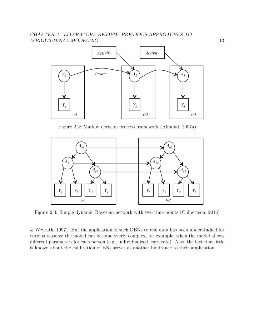
MDPs (Boutilier et al., 1999) have been often used to inform instructional decision makingby incorporating nodes that influence the transition between the time slices into the model.A MDP model contains (1) a set of possible states S, (2) a set of possible actions A, (3)the transition model T for each action’s effects in each state, (4) a reward structure of theactions and (5) a discount rate indicating the relative value of future compared to immediaterewards. LaMar (2017) discussed the use of a MDP to model students’ decision makingprocess for complex assessment tasks. Matsuda & VanLehn (2000) applied a MDP to makedecisions about selecting hints or new problems. Almond (2007a,b) employed a MDP tounderstand the effectiveness of an instruction and student learning. Figure 2.2 shows thegeneral framework of MDP presented in Almond (2007a). The transition from time t to timet+ 1 depends on activity variables (e.g., the choice of instruction). The student’s knowledgestates, A, are not observable so this model is called a partially observable Markov decisionprocess (POMDP).
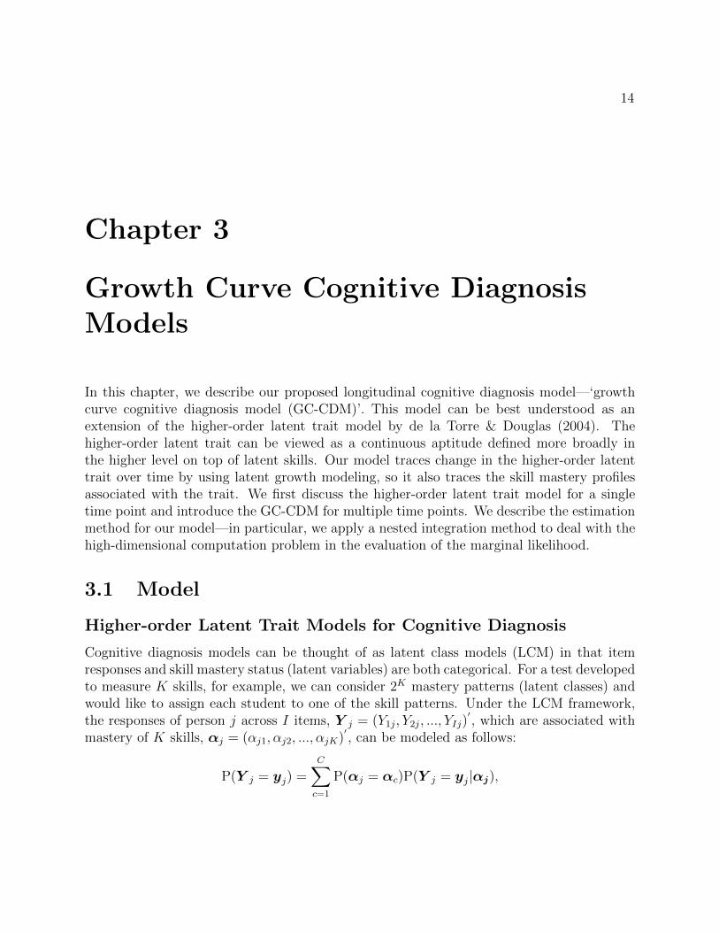
Culbertson (2016) discussed the possibility of more general DBNs with multiple latentskills. For example, Figure 2.3 represents a DBN with three skills (Aat, Abt, Act for t = 1, 2)measured at two time points. More complex temporal relationships can also be modeledsuch as the effect of change in one latent variable on other related latent variables (Schafer
CHAPTER 2. LITERATURE REVIEW: PREVIOUS APPROACHES TOLONGITUDINAL MODELING 13
A1
Y1
t=1
A2
Y2
t=2
A3
Y3
t=3
Growth
Activity Activity
Figure 2.2: Markov decision process framework (Almond, 2007a)
Ab1
Y1
t=1
Aa1
Ac1
Y2 Y3 Y4
Ab2
Y5
Aa2
Ac2
Y6 Y7 Y8
t=2
Figure 2.3: Simple dynamic Bayesian network with two time points (Culbertson, 2016)
& Weyrath, 1997). But the application of such DBNs to real data has been understudied forvarious reasons; the model can become overly complex, for example, when the model allowsdifferent parameters for each person (e.g., individualized learn rate). Also, the fact that littleis known about the calibration of BNs serves as another hindrance to their application.
14
Chapter 3
Growth Curve Cognitive DiagnosisModels
In this chapter, we describe our proposed longitudinal cognitive diagnosis model—‘growthcurve cognitive diagnosis model (GC-CDM)’. This model can be best understood as anextension of the higher-order latent trait model by de la Torre & Douglas (2004). Thehigher-order latent trait can be viewed as a continuous aptitude defined more broadly inthe higher level on top of latent skills. Our model traces change in the higher-order latenttrait over time by using latent growth modeling, so it also traces the skill mastery profilesassociated with the trait. We first discuss the higher-order latent trait model for a singletime point and introduce the GC-CDM for multiple time points. We describe the estimationmethod for our model—in particular, we apply a nested integration method to deal with thehigh-dimensional computation problem in the evaluation of the marginal likelihood.
3.1 Model
Higher-order Latent Trait Models for Cognitive Diagnosis
Cognitive diagnosis models can be thought of as latent class models (LCM) in that itemresponses and skill mastery status (latent variables) are both categorical. For a test developedto measure K skills, for example, we can consider 2K mastery patterns (latent classes) andwould like to assign each student to one of the skill patterns. Under the LCM framework,the responses of person j across I items, Y j = (Y1j, Y2j, ..., YIj)
′, which are associated with
mastery of K skills, αj = (αj1, αj2, ..., αjK)′, can be modeled as follows:
P(Y j = yj) =C∑c=1
P(αj = αc)P(Y j = yj|αj),
CHAPTER 3. GROWTH CURVE COGNITIVE DIAGNOSIS MODELS 15
where αc indicates the skill mastery pattern of latent class c and the sum is over all C = 2K
classes. Following the structural equation modeling convention, the first part of the model,P(αj = αc), is often called the structural component and the second part, P(Y j = yj|αj),is called the measurement component.
The measurement component can be rewritten by the local independence assumption:P(Y j = yj|αj) =
∏Ii=1 P(Yij = yij|αj). The measurement part of the DINA and DINO
models is described in Section 2.2. For the structural part, a structure for the K skillsshould be defined. The simplest assumption is the independence model which assumes thatthe skills are independent of each other:
P(αj) = P(αj1, αj2, ..., αjK) =K∏k=1
P(αjk).
The independence model has been considered in many studies due to its simplicity but thisassumption is usually implausible in practice. In some situations, it is likely that thereexists a higher order structure among the skills. For such cases, de la Torre & Douglas(2004) proposed a ‘higher-order latent trait model’. The model assumes that the skills arespecific knowledge related to one or more broadly defined constructs of general intelligenceor aptitude. This idea is reflected by introducing an item response model at a higher orderin which the latent skills (αj1, αj2, ..., αjK) play the role of items and are locally independentgiven the general aptitude, which is represented by θj.
Assuming that mastery of a set of skills of respondent j is related to an unidimensionaltrait θj, the probability model for αj conditional on θj is
P(αj|θj) =K∏k=1
P(αjk|θj),
where
P(αjk = 1|θj) =exp(λ0k + λ1kθj)
1 + exp(λ0k + λ1kθj). (3.1)
Here, λ0k and λ1k are higher order structural parameters resembling item “easiness” anddiscrimination parameters in IRT. Then, the marginal probability of the observed responsesof respondent j can be represented as:
P(Y j = yj) =
∫θj
{K∏k=1
P(αjk|θj)I∏i=1
P(Yij = yij|αj)
}P(θj)dθj.
In many applications, θj is assumed to be normally distributed with mean 0 and variance 1.Sometimes two-dimensional higher-order latent traits are used, but rarely higher-dimensional
CHAPTER 3. GROWTH CURVE COGNITIVE DIAGNOSIS MODELS 16
traits because, in general, the number of skills is much less than the number of items andneeds to be much greater than the dimension of θj for identifiability. When the measurementpart is defined as DINA, the model is called the higher-order DINA (HO-DINA) model.
Growth Curve Cognitive Diagnosis Models
Our proposed ‘growth curve cognitive diagnosis model (GC-CDM)’ extends the higher-orderlatent trait model to incorporate learning over time into cognitive diagnosis models. Assum-ing a respondent-specific linear relationships between time and the higher-order latent trait,respondent j’s changing latent trait over time can be modeled as latent growth curve modelwith respondent-specific random intercept and random slope of time. A similar approach toextend the HO-DINA model for longitudinal data was suggested by Ayers & Rabe-Hesketh(2011).
We consider a unidimensional latent trait for person j at occasion t, θjt, which is modeledas:
θjt = ζ1j + (β + ζ2j)× timejt + εjt, (3.2)
where timejt is the time associated with occasion t for respondent j, β is the mean slope oftime, ζ1j and ζ2j are the random intercept and random slope of time for person j respectively,and εjt is the time-specific error. It is assumed that(
ζ1jζ2j
)∼ N
[(00
),
(ψ11 ψ12
ψ21 ψ22
)], εjt ∼ N(0, σ2
t ) (3.3)
We can assume constant variance over time for εjt, i.e., σ2t = σ2. Given θjt, the probability
of skill profile αjt of person j at occasion t, is
P(αjt|θjt) =K∏k=1
P(αjkt|θjt),
where
P(αjkt = 1|θjt) =exp(λ0k + λ1kθjt)
1 + exp(λ0k + λ1kθjt). (3.4)
The higher-order structure parameters, λ0k and λ1k, are constant over time.For the measurement part, respondent j’s response Yijt to item i at time t, given his or
her skill profile and the higher-order trait at time t, can be modeled with the DINA model:
πijt = P(Yijt = 1|αjt, θjt) = (1− sit)ξijtg1−ξijtit , (3.5)
where ξijt is the indicator whether respondent j possesses all skills required by item i of theassessment administered at occasion t, and sit and git are slipping and guessing parameter of
CHAPTER 3. GROWTH CURVE COGNITIVE DIAGNOSIS MODELS 17
item i at occasion t, respectively. Different sets of items can be tested at different occasionsor the same items can be repeated at each occasion. For the latter, the number of items, It,are constant across occasions, It = I, and the guessing and slipping parameters of items areconstant over time.
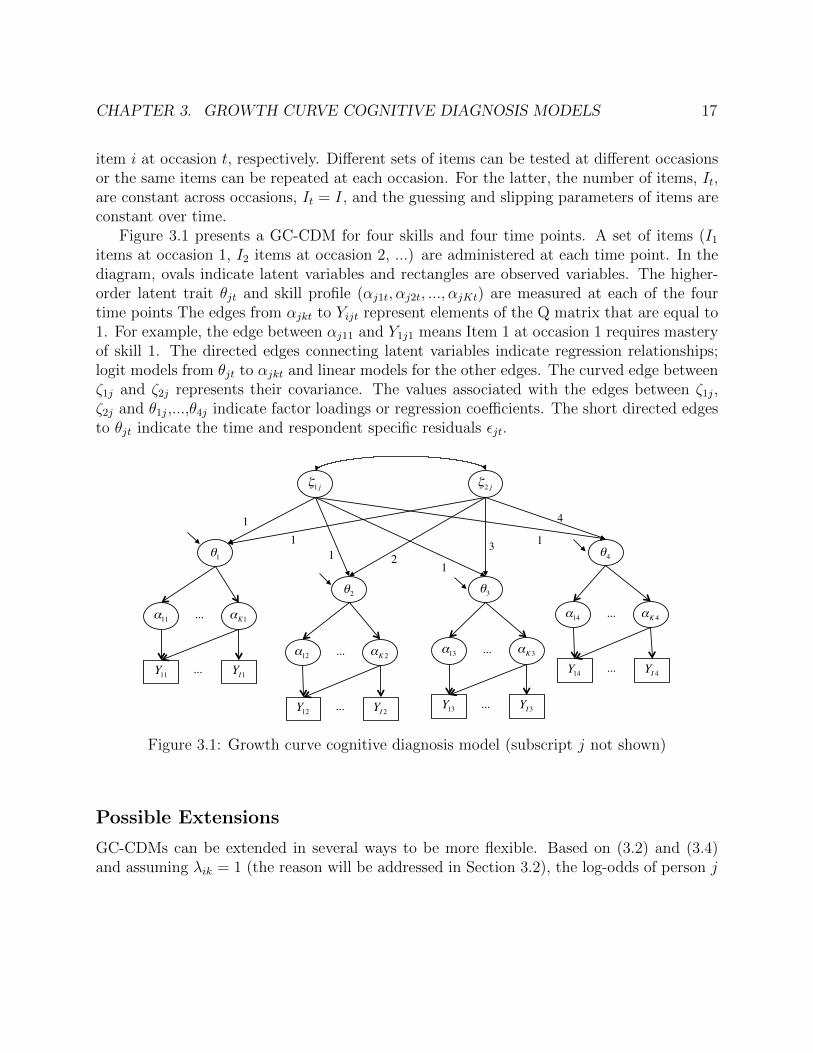
Figure 3.1 presents a GC-CDM for four skills and four time points. A set of items (I1items at occasion 1, I2 items at occasion 2, ...) are administered at each time point. In thediagram, ovals indicate latent variables and rectangles are observed variables. The higher-order latent trait θjt and skill profile (αj1t, αj2t, ..., αjKt) are measured at each of the fourtime points The edges from αjkt to Yijt represent elements of the Q matrix that are equal to1. For example, the edge between αj11 and Y1j1 means Item 1 at occasion 1 requires masteryof skill 1. The directed edges connecting latent variables indicate regression relationships;logit models from θjt to αjkt and linear models for the other edges. The curved edge betweenζ1j and ζ2j represents their covariance. The values associated with the edges between ζ1j,ζ2j and θ1j,...,θ4j indicate factor loadings or regression coefficients. The short directed edgesto θjt indicate the time and respondent specific residuals εjt.
ζ1 j ζ2 j
11
11
12
3
4
θ1
θ2 θ3
θ4
α11 αK1...
α12 αK 2... α13 αK3...
α14 αK 4...
Y11 YI1...
Y12 YI 2... Y13 YI3...
Y14 YI 4...
Figure 3.1: Growth curve cognitive diagnosis model (subscript j not shown)
Possible Extensions
GC-CDMs can be extended in several ways to be more flexible. Based on (3.2) and (3.4)and assuming λik = 1 (the reason will be addressed in Section 3.2), the log-odds of person j
CHAPTER 3. GROWTH CURVE COGNITIVE DIAGNOSIS MODELS 18
having skill k at occasion t can be written as follows:
logit(P(αjkt = 1|θjt)) = λ0k + θjt
= λ0k + ζ1j + (β + ζ2j)× timejt + εjt.
Here, the model assumes that the relationship between θjt and αjkt is constant over timeand that changes in the log-odds of mastering skill k per unit of time, represented β + ζ2j,are also constant over time. If the higher-order latent trait changes over time, the log-oddsof having each skill k changes by the same amount. However, the log-odds may changedifferently for different skills. For example, skill 1 may be learned faster than skill 2. GC-CDMs can be extended to allow different amounts of learning for each skill and each occasionby defining a skill and time specific intercept λ0kt instead of λ0k. λ0kt can be reparametrizedas λ0kt = λ0k + δkt, where δkt indicates time-specific deviation from the overall knowledgeof skill k. Some constraints would be necessary for the model to be identified. A naturalapproach would be to test for the necessity of including δkt for a given skill one skill at atime - similar to testing for differential item functioning in IRT. Alternatively, we can defineskill-specific linear growth with coefficients βk and remove β from the model.
In addition, GC-CDMs can be extended to incorporate respondents’ covariate informationto account for the effect of covariates on skill mastery. Ayers et al. (2013) proposed a methodto incorporate covariates into the DINA model, and the same approach can be applied toGC-CDMs. In GC-CDMs, the log-odds of person j having skill k at time t can be definedas follows: logit(P(αjkt = 1|θjt)) = λ0k + θjt + x
′jγ, where xj is a vector of covariates for
respondent j and γ is a vector of coefficients. The term x′jγ can alternatively be thought
of as part of θjt by adding this term to (3.2). The interpretation becomes that the meanhigher-order latent trait depends on covariates. By including interactions between covariatesand time, the mean growth in the higher-order trait can depend on covariates. The modelcan be further extended by including interactions between skills and covariates, representing“differential skill functioning”.
Although several extended GC-CDMs are available, the dissertation focuses on basicGC-CDMs.
3.2 Estimation
Maximum Marginal Likelihood Estimation
The marginal likelihood of the GC-CDM can be expressed as:
L(y) =J∏j=1
∫θj
{ T∏t=1
(P(αjt|θjt)
I∏i=1
P(yijt|αjt))}
P(θj)dθj, (3.6)
CHAPTER 3. GROWTH CURVE COGNITIVE DIAGNOSIS MODELS 19
where θj = (ζ1j, ζ2j, εj1, ..., εjT )T and P(θj) = P(ζ1j, ζ2j)∏T
t=1 P(εjt), a product of one bi-variate and T univariate densities as defined in (3.2). Evaluation of this likelihood requires(T + 2)-dimensional integration. The integral can be evaluated by numerical integrationtechniques (e.g., Gaussian quadrature), but an issue arises when the number of time pointincreases; the computational complexity increases exponentially.
As an alternative, we consider a dimension reduction technique using nested integrationbased on the fact that the εjt are independent across occasions. Then, the marginal likelihoodcan be reexpressed as:
L(y) =J∏j=1
∫ζ1j ,ζ2j
{ T∏t=1
∫εjt
(P(αjt|ζ1j, ζ2j, εjt)
I∏i=1
P(yijt|αjt))
P(εjt)dεjt
}P(ζ1j, ζ2j)dζ1jζ2j,
(3.7)This approach provides significant computational savings as the MLE requires only 3-dimensionalintegration regardless of the number of time points. Such nested integration was discussed in(Gibbons & Hedeker, 1992; Rijmen, 2009; Cai, 2010) for bifactor-type item response modelsand (Jeon & Rabe-Hesketh, 2016) for an autoregressive growth IRT model. This likelihoodhas the structure of the likelihood for a multilevel model in which occasions are nested withinpersons (occasions are units and persons are clusters). In contrast, the likelihood in (3.6)treats persons and the T occasions as being on the same level (multivariate perspective).
The marginal likelihood is maximized using the Expectation Maximization (EM) algo-rithm (Dempster et al., 1977). Details about the EM algorithm for DINA model estimationare discussed in de la Torre (2009). The Mplus software (version 8) (Muthen & Muthen,2017) was used to implement estimation of GC-CDMs.
Estimation of the Higher-order Structural Parameters
Prior to implementation of the GC-CDM, we developed Mplus codes for the HO-DINA modelfor a single occasion and applied it to a simulated data to confirm its feasibility. For thesimulation, responses of 1, 000 respondents to 20 items were generated. The slipping andguessing parameter values were randomly generated from a uniform distribution from 0.1 to0.3. The Q-matrix in Table 3.1 was used.
The IRT model for the higher-order joint skill distribution defined in (3.1) can be specifiedas a two-parameter logistic (2PL) or a Rasch model. For the 2PL model, the followingvalues were used for the higher-order structural parameters: λ0 = (λ01, λ02, λ03, λ04)
′=
(1.51,−1.42,−0.66, 0.50)′
and λ1 = (λ11, λ12, λ13, λ14)′
= (1.34, 0.65, 1.11, 0.97)′. For the
Rasch model, the slopes λ1 were fixed to 1. The higher-order latent traits were assumed tobe normally distributed with mean 0 and variance 1. The R codes for generating data arein Appendix.
CHAPTER 3. GROWTH CURVE COGNITIVE DIAGNOSIS MODELS 20
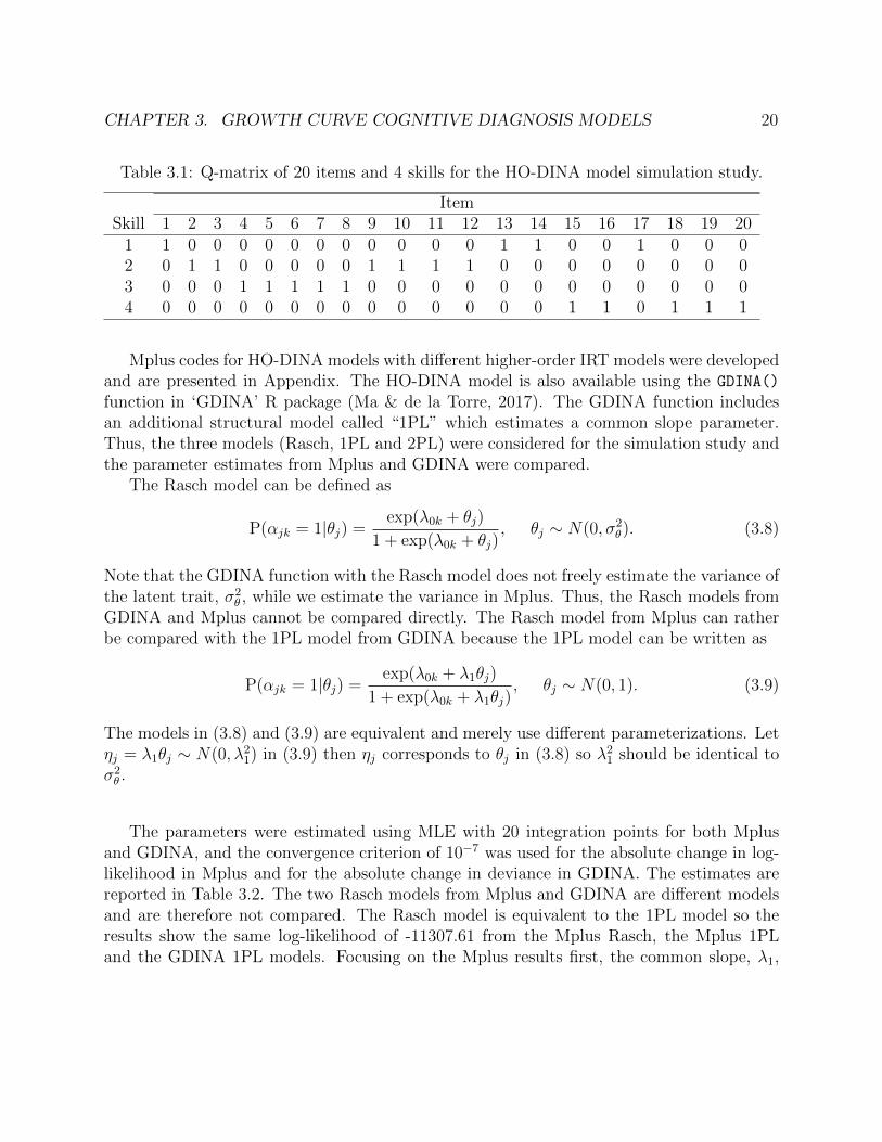
Table 3.1: Q-matrix of 20 items and 4 skills for the HO-DINA model simulation study.
ItemSkill 1 2 3 4 5 6 7 8 9 10 11 12 13 14 15 16 17 18 19 20
1 1 0 0 0 0 0 0 0 0 0 0 0 1 1 0 0 1 0 0 02 0 1 1 0 0 0 0 0 1 1 1 1 0 0 0 0 0 0 0 03 0 0 0 1 1 1 1 1 0 0 0 0 0 0 0 0 0 0 0 04 0 0 0 0 0 0 0 0 0 0 0 0 0 0 1 1 0 1 1 1
Mplus codes for HO-DINA models with different higher-order IRT models were developedand are presented in Appendix. The HO-DINA model is also available using the GDINA()
function in ‘GDINA’ R package (Ma & de la Torre, 2017). The GDINA function includesan additional structural model called “1PL” which estimates a common slope parameter.Thus, the three models (Rasch, 1PL and 2PL) were considered for the simulation study andthe parameter estimates from Mplus and GDINA were compared.
The Rasch model can be defined as
P(αjk = 1|θj) =exp(λ0k + θj)
1 + exp(λ0k + θj), θj ∼ N(0, σ2
θ). (3.8)
Note that the GDINA function with the Rasch model does not freely estimate the variance ofthe latent trait, σ2
θ , while we estimate the variance in Mplus. Thus, the Rasch models fromGDINA and Mplus cannot be compared directly. The Rasch model from Mplus can ratherbe compared with the 1PL model from GDINA because the 1PL model can be written as
P(αjk = 1|θj) =exp(λ0k + λ1θj)
1 + exp(λ0k + λ1θj), θj ∼ N(0, 1). (3.9)
The models in (3.8) and (3.9) are equivalent and merely use different parameterizations. Letηj = λ1θj ∼ N(0, λ21) in (3.9) then ηj corresponds to θj in (3.8) so λ21 should be identical toσ2θ .
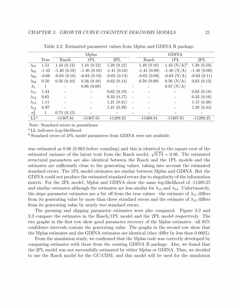
The parameters were estimated using MLE with 20 integration points for both Mplusand GDINA, and the convergence criterion of 10−7 was used for the absolute change in log-likelihood in Mplus and for the absolute change in deviance in GDINA. The estimates arereported in Table 3.2. The two Rasch models from Mplus and GDINA are different modelsand are therefore not compared. The Rasch model is equivalent to the 1PL model so theresults show the same log-likelihood of -11307.61 from the Mplus Rasch, the Mplus 1PLand the GDINA 1PL models. Focusing on the Mplus results first, the common slope, λ1,
CHAPTER 3. GROWTH CURVE COGNITIVE DIAGNOSIS MODELS 21
Table 3.2: Estimated parameter values from Mplus and GDINA R package.
Mplus GDINATrue Rasch 1PL 2PL Rasch 1PL 2PL
λ01 1.51 1.44 (0.12) 1.44 (0.12) 1.28 (0.12) 1.49 (0.10) 1.43 (N/A)b 1.28 (0.10)λ02 -1.42 -1.40 (0.10) -1.40 (0.10) -1.41 (0.10) -1.45 (0.09) -1.40 (N/A) -1.40 (0.09)λ03 -0.66 -0.63 (0.10) -0.63 (0.10) -0.65 (0.13) -0.65 (0.09) -0.63 (N/A) -0.63 (0.11)λ04 0.50 0.56 (0.10) 0.56 (0.10) 0.62 (0.14) 0.58 (0.09) 0.56 (N/A) 0.63 (0.13)λ1 1 - 0.86 (0.09) - - - 0.87 (N/A) -λ11 1.34 - - 0.62 (0.19) - - - 0.62 (0.18)λ12 0.65 - - 0.33 (0.17) - - - 0.33 (0.16)λ13 1.11 - - 1.21 (0.41) - - - 1.15 (0.38)λ14 0.97 - - 1.21 (0.39) - - - 1.28 (0.44)σ2θ 1 0.74 (0.15) - - - - - -
LLa -11307.61 -11307.61 -11289.25 -11308.81 -11307.61 -11289.25
Note: Standard errors in parenthesesa LL indicates Log-likelihoodb Standard errors of 1PL model parameters from GDINA were not available.
was estimated as 0.86 (0.863 before rounding) and this is identical to the square root of theestimated variance of the latent trait from the Rasch model,
√0.74 = 0.86. The estimated
structural parameters are also identical between the Rasch and the 1PL models and theestimates are sufficiently close to the generating values, taking into account the estimatedstandard errors. The 1PL model estimates are similar between Mplus and GDINA. But theGDINA could not produce the estimated standard errors due to singularity of the informationmatrix. For the 2PL model, Mplus and GDINA show the same log-likelihood of -11289.25and similar estimates although the estimates are less similar for λ13 and λ14. Unfortunately,the slope parameter estimates are a bit off from the true values—the estimate of λ11 differsfrom its generating value by more than three standard errors and the estimate of λ12 differsfrom its generating value by nearly two standard errors.
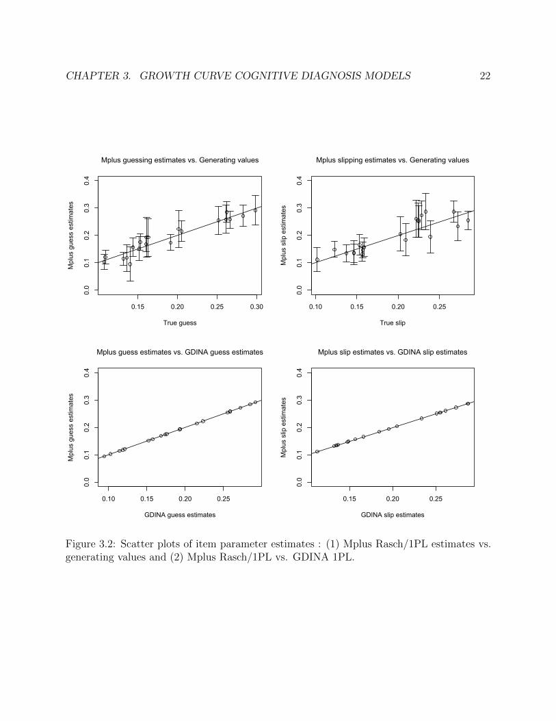
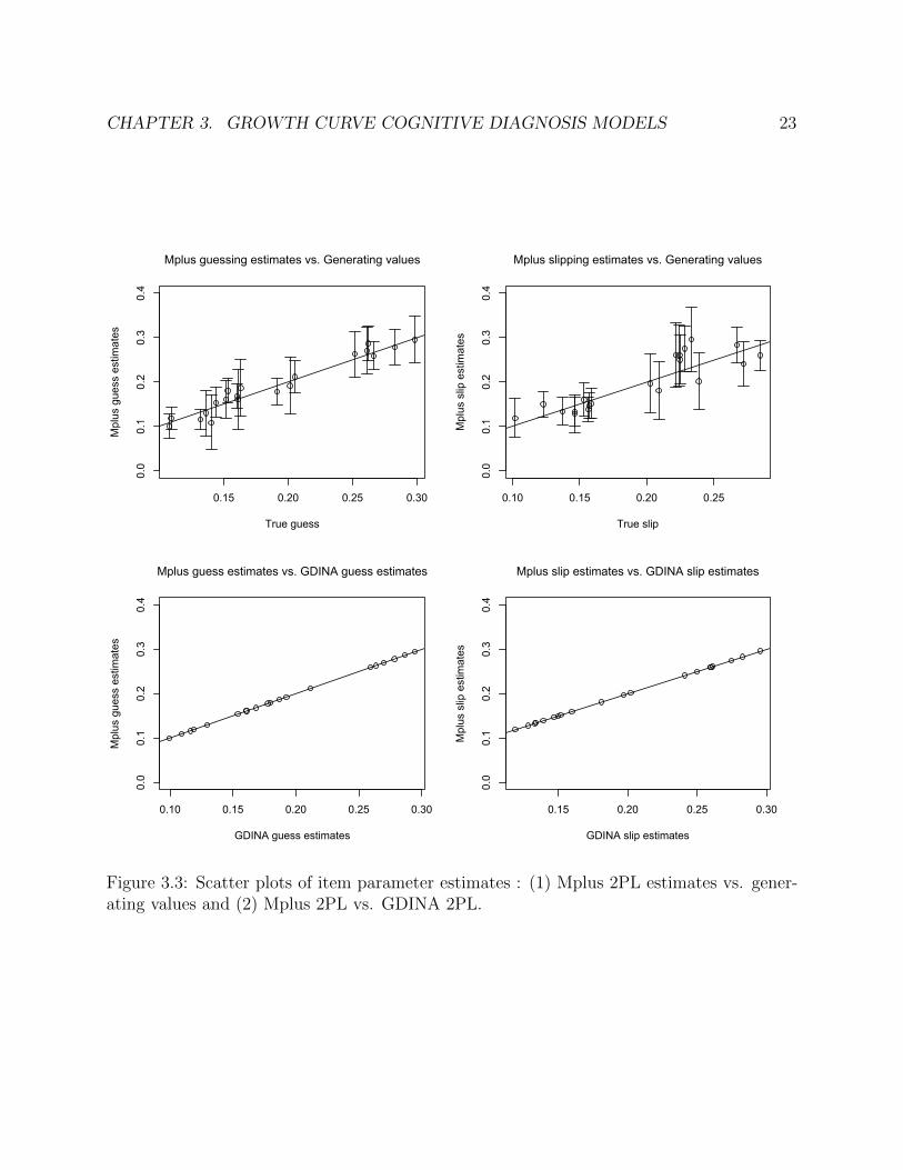
The guessing and slipping parameter estimates were also compared. Figure 3.2 and3.3 compare the estimates in the Rasch/1PL model and the 2PL model respectively. Thetwo graphs in the first row show good parameter recovery of the Mplus estimates—all 95%confidence intervals contain the generating value. The graphs in the second row show thatthe Mplus estimates and the GDINA estimates are identical (they differ by less than 0.0005).
From the simulation study, we confirmed that the Mplus code was correctly developed bycomparing estimates with those from the existing GDINA R package. Also, we found thatthe 2PL model was not successfully estimated by either Mplus or GDINA. Thus, we decidedto use the Rasch model for the GC-CDM, and this model will be used for the simulation
CHAPTER 3. GROWTH CURVE COGNITIVE DIAGNOSIS MODELS 22
0.15 0.20 0.25 0.30
0.0
0.1
0.2
0.3
0.4
True guess
Mpl
us g
uess
est
imat
es
Mplus guessing estimates vs. Generating values
0.10 0.15 0.20 0.250.0
0.1
0.2
0.3
0.4
True slip
Mpl
us s
lip e
stim
ates
Mplus slipping estimates vs. Generating values
0.10 0.15 0.20 0.25
0.0
0.1
0.2
0.3
0.4
GDINA guess estimates
Mpl
us g
uess
est
imat
es
Mplus guess estimates vs. GDINA guess estimates
0.15 0.20 0.25
0.0
0.1
0.2
0.3
0.4
GDINA slip estimates
Mpl
us s
lip e
stim
ates
Mplus slip estimates vs. GDINA slip estimates
Figure 3.2: Scatter plots of item parameter estimates : (1) Mplus Rasch/1PL estimates vs.generating values and (2) Mplus Rasch/1PL vs. GDINA 1PL.
CHAPTER 3. GROWTH CURVE COGNITIVE DIAGNOSIS MODELS 23
0.15 0.20 0.25 0.30
0.0
0.1
0.2
0.3
0.4
True guess
Mpl
us g
uess
est
imat
es
Mplus guessing estimates vs. Generating values
0.10 0.15 0.20 0.250.0
0.1
0.2
0.3
0.4
True slip
Mpl
us s
lip e
stim
ates
Mplus slipping estimates vs. Generating values
0.10 0.15 0.20 0.25 0.30
0.0
0.1
0.2
0.3
0.4
GDINA guess estimates
Mpl
us g
uess
est
imat
es
Mplus guess estimates vs. GDINA guess estimates
0.15 0.20 0.25 0.30
0.0
0.1
0.2
0.3
0.4
GDINA slip estimates
Mpl
us s
lip e
stim
ates
Mplus slip estimates vs. GDINA slip estimates
Figure 3.3: Scatter plots of item parameter estimates : (1) Mplus 2PL estimates vs. gener-ating values and (2) Mplus 2PL vs. GDINA 2PL.
CHAPTER 3. GROWTH CURVE COGNITIVE DIAGNOSIS MODELS 24
studies and empirical studies in the next chapters.
3.3 Model when the Number of Occasions is Two
When only two time points are available (T = 2) and the timing is identical across subjects,timejt = timet, the growth curve model in (3.2) is not identified. For such case, we let thehigher-order latent traits at occasion 1 and occasion 2 be correlated with each other ratherthan specifying a linear growth curve model. The correlation between θj1 and θj2 is modeledby using a bivariate normal distribution:(
θj1θj2
)∼ N
[(µ1
µ2
),
(σ21 σ12
σ21 σ22
)],
where (µ1, µ2)′is the mean vector of the higher-order latent traits; σ2
1 and σ22 are the variances
of θj1 and θj2 respectively; and σ12 (=σ21) is the covariance between θj1 and θj2.For the higher-order IRT model, we used the Rasch model:
P(αjkt = 1|θjt) =exp(λ0k + θjt)
1 + exp(λ0k + θjt),
where λ0k is constant over time.This approach is similar to Andersen’s longitudinal Rasch model described in Section 2.1
in that both models use a bivariate normal distribution to allow correlation between latenttraits over time. To measure individual growth between two occasions, we can calculate thedifference between predicted latent traits at each time point.
25
Chapter 4
Simulation Study
Two simulation studies were conducted to investigate how well the parameters of the growthcurve DINA (GC-DINA) model can be recovered by the estimation method described inChapter 3. The first simulation study focuses on parameter recovery under differing conditions—three factors were manipulated: the number of respondents, the design of the Q-matrix andthe number of time points. The second simulation study focuses on the analysis of pre-postassessment data when only two time points are available.
4.1 Simulation Study 1
Simulation Conditions
In this section, we examine parameter recovery of the GC-DINA using maximum marginallikelihood estimation with the nested integration described in Section 3.2. Parameter recov-ery was investigated under various conditions. In particular, we manipulated three factors:the number of respondents, the design of the Q-matrix and the number of time points. ForCDMs, in general, it has been recognized that the design of the Q-matrix is an importantfactor in model estimation. We especially considered the complexity of the Q-matrix whichdepends on the number of items measuring each skill, the number of skills each item measuresand the number of skills that are measured jointly with other skills. Madison & Bradshaw(2015) demonstrated the effect of the Q-matrix design on classification accuracy for thelog-linear cognitive diagnosis model. Their study showed that classification accuracy for agiven skill increases as the number of items measuring that skill only increases, whereas theaccuracy deteriorates when the item measuring that skill tend to also measure other skillsin conjunction.
Estimation time for the GC-DINA model is considerable, so it was not feasible to conduct

CHAPTER 4. SIMULATION STUDY 26
a full factorial design with multiple replicates per combination of conditions. By varying thenumber of respondents, the design of the Q-matrix and the number of time points, weconsidered the following six models:
• Model 1: 1,000 respondents & Simple Q-matrix & Three time points
• Model 2: 1,000 respondents & Complex Q-matrix & Three time points
• Model 3: 500 respondents & Simple Q-matrix & Three time points
• Model 4: 500 respondents & Complex Q-matrix & Three time points
• Model 5: 500 respondents & Simple Q-matrix & Four time points
• Model 6: 500 respondents & Complex Q-matrix & Four time points
We chose these models so that we can investigate the effect of changing one factor at a time.We first considered Model 1 and Model 2 to examine the effect of the design of the Q-matrix.Next, we decreased the number of respondents to examine the effect of sample size (Model3 and Model 4). We then increased the number of time points to investigate the effect ofnumber of time points (Model 5 and Model 6).
Simple Q-matrix vs. Complex Q-matrix
Table 4.1 and 4.2 present the simple and complex Q-matrix used for the simulation, respec-tively. In the simple Q-matrix, each item measures only one skill. The number of items thatmeasure each skill is as follows: 4 items for Skill 1, 6 items for Skill 2, 5 items for Skill 3,and 5 items for Skill 4. In the complex Q-matrix, 7 items out of 20 measure a single skill:item 1, 2, 17, 18 and 19 measure Skill 1 in isolation; item 9 measures only Skill 2; and item13 measures only Skill 3. There is no item that measures only Skill 4. 10 items measure twoskills jointly, and 3 items measure all four skills. In terms of the number of items that mea-sure each skill, the skills (Skill 1 - Skill 4) are measured by 16 items, 12 items, 5 items and 6items respectively. Both the simple Q-matrix and complex Q-matrix were derived from thereal application of Enhanced Anchored Instruction (EAI; Bottge et al., 2003). Thus, theseQ-matrices reflect practical cognitive diagnostic assessment. For the simple Q-matrix, weused the Q-matrix developed for the Problem Solving Test (PST) (Bottge et al., 2014, 2015).The complex Q-matrix was derived from the Q-matrix developed for the Fraction of the Cost(FOC) test (Bottge et al., 2007; Li et al., 2016). The FOC test has 23 items and 4 skills.We deleted three items that measure all of the four skills from the original Q-matrix, so theQ-matrix has 20 items (to be comparable to the simple Q-matrix). By taking three itemsout, estimation becomes more challenging because there is less information about the latent
CHAPTER 4. SIMULATION STUDY 27
skills. Real data with the original versions of the Q-matrices will be used in the empiricalstudy and more details about the Q-matrices will be discussed in Chapter 5.
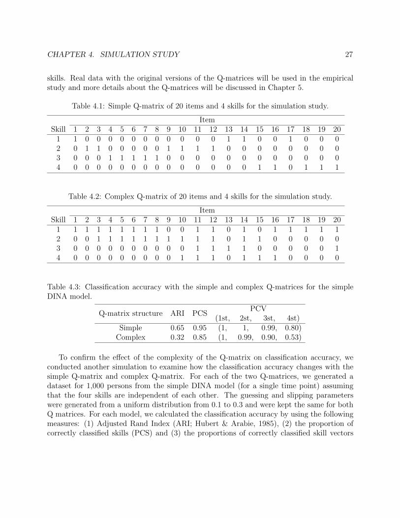
Table 4.1: Simple Q-matrix of 20 items and 4 skills for the simulation study.
ItemSkill 1 2 3 4 5 6 7 8 9 10 11 12 13 14 15 16 17 18 19 20
1 1 0 0 0 0 0 0 0 0 0 0 0 1 1 0 0 1 0 0 02 0 1 1 0 0 0 0 0 1 1 1 1 0 0 0 0 0 0 0 03 0 0 0 1 1 1 1 1 0 0 0 0 0 0 0 0 0 0 0 04 0 0 0 0 0 0 0 0 0 0 0 0 0 0 1 1 0 1 1 1
Table 4.2: Complex Q-matrix of 20 items and 4 skills for the simulation study.
ItemSkill 1 2 3 4 5 6 7 8 9 10 11 12 13 14 15 16 17 18 19 20
1 1 1 1 1 1 1 1 1 0 0 1 1 0 1 0 1 1 1 1 12 0 0 1 1 1 1 1 1 1 1 1 1 0 1 1 0 0 0 0 03 0 0 0 0 0 0 0 0 0 0 1 1 1 1 0 0 0 0 0 14 0 0 0 0 0 0 0 0 0 1 1 1 0 1 1 1 0 0 0 0
Table 4.3: Classification accuracy with the simple and complex Q-matrices for the simpleDINA model.
Q-matrix structure ARI PCSPCV
(1st, 2st, 3st, 4st)Simple 0.65 0.95 (1, 1, 0.99, 0.80)
Complex 0.32 0.85 (1, 0.99, 0.90, 0.53)
To confirm the effect of the complexity of the Q-matrix on classification accuracy, weconducted another simulation to examine how the classification accuracy changes with thesimple Q-matrix and complex Q-matrix. For each of the two Q-matrices, we generated adataset for 1,000 persons from the simple DINA model (for a single time point) assumingthat the four skills are independent of each other. The guessing and slipping parameterswere generated from a uniform distribution from 0.1 to 0.3 and were kept the same for bothQ matrices. For each model, we calculated the classification accuracy by using the followingmeasures: (1) Adjusted Rand Index (ARI; Hubert & Arabie, 1985), (2) the proportion ofcorrectly classified skills (PCS) and (3) the proportions of correctly classified skill vectors
CHAPTER 4. SIMULATION STUDY 28
(PCV). The ARI has been used as a common measure of agreement between two partitions,and it is defined as the number of agreement between two partitions divided by the totalnumber of pairs of objects. The ARI lies between 0 and 1, where 1 indicates perfect agree-ment. The PCS is the skill level correct classification accuracy rate, while the PCV is thevector level correct classification rate. The PCV is a vector with four elements—the firstelement is the proportion of at least one skill in the vector being correctly classified; thesecond element is the proportion of at least two skills being correctly classified; the third el-ement is the proportion of at least three skills being correctly classified; and the last elementis the proportion of all elements in the vector being correctly classified. The calculation ofthe ARI is available using adjustedRandIndex() function in the ‘mclust’ R package. ThePCS and PCV can be obtained from the ClassRate() function in the ‘GDINA’ R package.The R code for generating two simulated data sets from the DINA model and calculatingthe accuracy measures are in Appendix.
Table 4.3 shows the calculated classification accuracy rates. The AIRs were 0.65 for thesimple Q-matrix and 0.32 for the complex Q-matrix. The PCSs were 0.95 for the simpleQ-matrix and 0.85 for the complex Q-matrix. In the PCV elements, a large differencewas observed in the 4th element which indicates the proportion of correctly identified skillmastery profiles across all the four skills: 0.80 for the simple Q-matrix and 0.53 for thecomplex matrix. This suggests that the prediction of skill mastery profiles suffers as thecomplexity of the Q-matrix increases in the independence DINA model.
Data Generation & Analysis
For all of the six models, we generated response data for 20 items and 4 skills. The guessingand slipping parameters, gi, si (i = 1, ..., 20), were randomly generated from a uniformdistribution from 0.1 to 0.3, and were constant over time. The same set of guessing andslipping parameters were used across the six models. To simulate the higher-order latenttrait, we used the following generating values: the variance of the random intercept ψ11 = 0.4,the variance of the random slope of time ψ22 = 0.02, the covariance between the randomintercept and random slope ψ12 = ψ21 = 0.02, the average growth β = 0.3, and the varianceof the occasion-specific error σ2 = 0.6. For the higher-order structural parameters, we usedλ0 = (λ01, λ02, λ03, λ04) = (1.51,−1.42,−0.66, 0.50). We used the same generated values forthe higher-order latent traits and skill mastery indicators between Model 1 and 2, betweenModel 3 and 4, and between Model 5 and 6 by using the same seed number. Then, thecomparison of models with different Q-matrices can be more legitimate as we rule out thechance error that occurs in generating latent variables. Time was coded as 0,1,2 for threeoccasions and 0,1,2,3 for four occasions. The R codes generating six data sets are availablein Appendix.
CHAPTER 4. SIMULATION STUDY 29
The six GC-DINA models were fitted in Mplus. As discussed in Section 3.2, when usingthe nested integration approach, the likelihood has the structure of the multilevel model—theoccasions are nested within respondents. We implemented the GC-DINA model in Mplususing the multilevel approach. Note that the multivariate approach based on (3.6) was notfeasible in Mplus due to high dimensions—the evaluation of the likelihood requires (T+2)-dimensional integration. We used 15 integration points and the convergence criterion of 10−7
for the absolute change in the log-likelihood. The Mplus codes for the GC-DINA models arein Appendix.
In addition to comparing GC-DINA estimates with generating values, we compared themwith estimates that would be obtained if latent variables in the model could be observeddirectly. A best-case scenario for estimating the covariance matrix of the random interceptand slope would be that the random intercepts and slopes, ζ1j and ζ2j, are observed. Thiswas the first comparison. Moving one level down in the model, if the occasion-specific latenttraits, θjt, are observed, we could estimate a linear growth curve model; the model can bedefined as the same as in (3.2) but is fitted to the observed θjt. If we don’t observe thehigher-order latent traits but observe the skill mastery indicators, moving down one morelevel, then we could estimate the mixed-effects logistic model. The model has a three-levelstructure, where the skill mastery indicators (level 1) are nested within occasions (level 2)and occasions are nested within persons (level 3). The model can be expressed as:
logit(P(αjkt = 1|s1k, s2k, s3k, s4k, timet, ζ1j, ζ2j, εjt))
= λ01s1k + λ02s2k + λ03s3k + λ04s4k + (β + ζ2j)timet + ζ1j + εjt,(4.1)
where s1k, s2k, s3k, s4k are dummy variables for αjkt representing mastery of Skill 1, Skill 2,Skill 3 and Skill 4, respectively (i.e., s1k = 1 when k = 1 and 0 otherwise.); timet is the timeassociated with occasion t; ζ1j and ζ2j are the random intercept and random slope of timefor person j respectively; and εjt is the occasion-specific random intercept. It is assumedthat (
ζ1jζ2j
)∼ N
[(00
),
(ψ11 ψ12
ψ21 ψ22
)], εjt ∼ N(0, σ2). (4.2)
The scenarios with observed latent variables—(1) the covariance matrix calculated fromobserved random effects, ζ1j, ζ2j, (2) the growth curve model with observed higher-orderlatent traits, θjt, and (3) the mixed-effects logistic model with observed skill mastery indica-tors, αjkt—should be better cases than the GC-DINA model with observed item responses,Yijt, thus the GC-DINA model estimates are not expected to be better than the estimatesobtained from the scenarios (1) to (3).
We investigated how the GC-DINA estimates deteriorate due to having only the indirectinformation about the skill and the higher-order latent traits in terms of point estimates
CHAPTER 4. SIMULATION STUDY 30
and the standard errors. To compare the standard errors with less rounding (the estimatedstandard errors will be reported after being rounded to 2 decimal points), we calculated thesquare root of relative efficiency (= the ratio between standard errors) to examine how muchstandard errors increase in the GC-DINA model compared to the growth curve model andthe mixed effects logistic model.
Results
The Effect of Design of the Q-matrix
We first focus on comparison between Model 1 and Model 2 to examine how the estimateschange depending on the complexity of the Q-matrix. The estimated parameters for Model1 and Model 2 are shown in Table 4.4. In Model 1, the estimates for the GC-DINA modelsuccessfully recovered the generating values—the difference is less than one standard errorexcept for λ04 (the difference for λ04 is only slightly greater than one standard error). Also,the point estimates of the GC-DINA model were not much worse than the estimates fromthe observed random effects (‘Observed’), the growth curve model (‘Growth Curve’) and themixed-effects logistic model (‘Mixed Logit’).
In Model 2, the point estimates of the GC-DINA model, however, deteriorated for someparameters. We can consider this deterioration in the point estimates as the effect of thecomplex Q-matrix since the generated latent variables were the same between Model 1 andModel 2 (accordingly, the estimates for other models were the same between Model 1 andModel 2). In particular, the point estimates of ψ11 and ψ12 became worse as ψ11 = 0.32 andψ12 = 0.08 in Model 2 while the generating values were ψ11 = 0.40 and ψ12 = 0.02. Butinterestingly, this was not reflected in the standard errors—the standard errors for ψ11 and ψ12
were nearly the same between Model 1 and Model 2. On the other hand, for σ2, the standarderror increased from 0.10 (Model 1) to 0.18 (Model 2) while the point estimates remainedthe same. The inconsistency between the point estimates and the standard errors may haveoccurred because we used the estimated standard errors, not true sampling variances andthere is a risk that this estimated standard errors computed by Mplus might not be goodenough. For λ03 and λ04, both of the point estimates and the standard errors became worse.In Model 1, λ03 = −0.61 with a standard error of 0.07 and λ04 = 0.59 with a standard errorof 0.08. In Model 2, however, they became λ03 = −0.78 with a standard error of 0.15 andλ04 = 0.66 with a standard error of 0.17. This can be partly explained by the fact thatthe complex Q-matrix has no item that measures only Skill 4 and the smaller number ofitems that measure each of Skill 3 and Skill 4: Skill 3 is measured by 5 items and Skill 4is measured by 6 items whereas Skill 1 and Skill 2 are measured by 16 items and 12 items,respectively.
Next, we compared Model 3 with Model 4 to investigate the effect of the Q-matrix
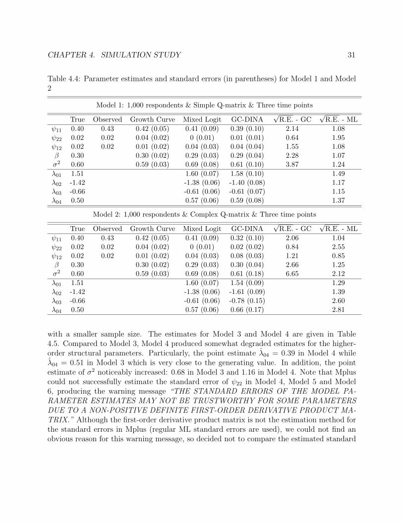
CHAPTER 4. SIMULATION STUDY 31
Table 4.4: Parameter estimates and standard errors (in parentheses) for Model 1 and Model2
Model 1: 1,000 respondents & Simple Q-matrix & Three time points
True Observed Growth Curve Mixed Logit GC-DINA√
R.E. - GC√
R.E. - ML
ψ11 0.40 0.43 0.42 (0.05) 0.41 (0.09) 0.39 (0.10) 2.14 1.08ψ22 0.02 0.02 0.04 (0.02) 0 (0.01) 0.01 (0.01) 0.64 1.95ψ12 0.02 0.02 0.01 (0.02) 0.04 (0.03) 0.04 (0.04) 1.55 1.08β 0.30 0.30 (0.02) 0.29 (0.03) 0.29 (0.04) 2.28 1.07σ2 0.60 0.59 (0.03) 0.69 (0.08) 0.61 (0.10) 3.87 1.24
λ01 1.51 1.60 (0.07) 1.58 (0.10) 1.49λ02 -1.42 -1.38 (0.06) -1.40 (0.08) 1.17λ03 -0.66 -0.61 (0.06) -0.61 (0.07) 1.15λ04 0.50 0.57 (0.06) 0.59 (0.08) 1.37
Model 2: 1,000 respondents & Complex Q-matrix & Three time points
True Observed Growth Curve Mixed Logit GC-DINA√
R.E. - GC√
R.E. - ML
ψ11 0.40 0.43 0.42 (0.05) 0.41 (0.09) 0.32 (0.10) 2.06 1.04ψ22 0.02 0.02 0.04 (0.02) 0 (0.01) 0.02 (0.02) 0.84 2.55ψ12 0.02 0.02 0.01 (0.02) 0.04 (0.03) 0.08 (0.03) 1.21 0.85β 0.30 0.30 (0.02) 0.29 (0.03) 0.30 (0.04) 2.66 1.25σ2 0.60 0.59 (0.03) 0.69 (0.08) 0.61 (0.18) 6.65 2.12
λ01 1.51 1.60 (0.07) 1.54 (0.09) 1.29λ02 -1.42 -1.38 (0.06) -1.61 (0.09) 1.39λ03 -0.66 -0.61 (0.06) -0.78 (0.15) 2.60λ04 0.50 0.57 (0.06) 0.66 (0.17) 2.81
with a smaller sample size. The estimates for Model 3 and Model 4 are given in Table4.5. Compared to Model 3, Model 4 produced somewhat degraded estimates for the higher-order structural parameters. Particularly, the point estimate λ04 = 0.39 in Model 4 whileλ04 = 0.51 in Model 3 which is very close to the generating value. In addition, the pointestimate of σ2 noticeably increased: 0.68 in Model 3 and 1.16 in Model 4. Note that Mpluscould not successfully estimate the standard error of ψ22 in Model 4, Model 5 and Model6, producing the warning message “THE STANDARD ERRORS OF THE MODEL PA-RAMETER ESTIMATES MAY NOT BE TRUSTWORTHY FOR SOME PARAMETERSDUE TO A NON-POSITIVE DEFINITE FIRST-ORDER DERIVATIVE PRODUCT MA-TRIX.” Although the first-order derivative product matrix is not the estimation method forthe standard errors in Mplus (regular ML standard errors are used), we could not find anobvious reason for this warning message, so decided not to compare the estimated standard
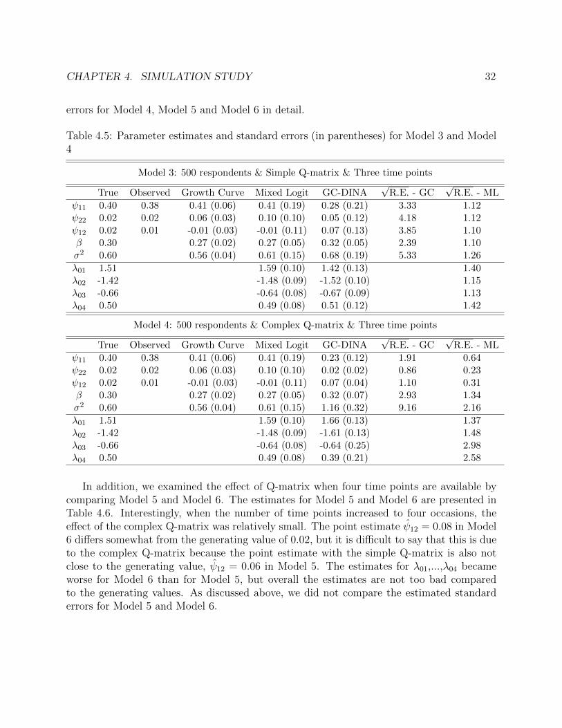
CHAPTER 4. SIMULATION STUDY 32
errors for Model 4, Model 5 and Model 6 in detail.
Table 4.5: Parameter estimates and standard errors (in parentheses) for Model 3 and Model4
Model 3: 500 respondents & Simple Q-matrix & Three time points
True Observed Growth Curve Mixed Logit GC-DINA√
R.E. - GC√
R.E. - ML
ψ11 0.40 0.38 0.41 (0.06) 0.41 (0.19) 0.28 (0.21) 3.33 1.12ψ22 0.02 0.02 0.06 (0.03) 0.10 (0.10) 0.05 (0.12) 4.18 1.12ψ12 0.02 0.01 -0.01 (0.03) -0.01 (0.11) 0.07 (0.13) 3.85 1.10β 0.30 0.27 (0.02) 0.27 (0.05) 0.32 (0.05) 2.39 1.10σ2 0.60 0.56 (0.04) 0.61 (0.15) 0.68 (0.19) 5.33 1.26
λ01 1.51 1.59 (0.10) 1.42 (0.13) 1.40λ02 -1.42 -1.48 (0.09) -1.52 (0.10) 1.15λ03 -0.66 -0.64 (0.08) -0.67 (0.09) 1.13λ04 0.50 0.49 (0.08) 0.51 (0.12) 1.42
Model 4: 500 respondents & Complex Q-matrix & Three time points
True Observed Growth Curve Mixed Logit GC-DINA√
R.E. - GC√
R.E. - ML
ψ11 0.40 0.38 0.41 (0.06) 0.41 (0.19) 0.23 (0.12) 1.91 0.64ψ22 0.02 0.02 0.06 (0.03) 0.10 (0.10) 0.02 (0.02) 0.86 0.23ψ12 0.02 0.01 -0.01 (0.03) -0.01 (0.11) 0.07 (0.04) 1.10 0.31β 0.30 0.27 (0.02) 0.27 (0.05) 0.32 (0.07) 2.93 1.34σ2 0.60 0.56 (0.04) 0.61 (0.15) 1.16 (0.32) 9.16 2.16
λ01 1.51 1.59 (0.10) 1.66 (0.13) 1.37λ02 -1.42 -1.48 (0.09) -1.61 (0.13) 1.48λ03 -0.66 -0.64 (0.08) -0.64 (0.25) 2.98λ04 0.50 0.49 (0.08) 0.39 (0.21) 2.58
In addition, we examined the effect of Q-matrix when four time points are available bycomparing Model 5 and Model 6. The estimates for Model 5 and Model 6 are presented inTable 4.6. Interestingly, when the number of time points increased to four occasions, theeffect of the complex Q-matrix was relatively small. The point estimate ψ12 = 0.08 in Model6 differs somewhat from the generating value of 0.02, but it is difficult to say that this is dueto the complex Q-matrix because the point estimate with the simple Q-matrix is also notclose to the generating value, ψ12 = 0.06 in Model 5. The estimates for λ01,...,λ04 becameworse for Model 6 than for Model 5, but overall the estimates are not too bad comparedto the generating values. As discussed above, we did not compare the estimated standarderrors for Model 5 and Model 6.
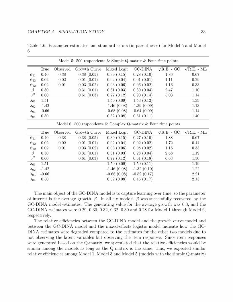
CHAPTER 4. SIMULATION STUDY 33
Table 4.6: Parameter estimates and standard errors (in parentheses) for Model 5 and Model6
Model 5: 500 respondents & Simple Q-matrix & Four time points
True Observed Growth Curve Mixed Logit GC-DINA√
R.E. - GC√
R.E. - ML
ψ11 0.40 0.38 0.38 (0.05) 0.39 (0.15) 0.28 (0.10) 1.86 0.67ψ22 0.02 0.02 0.01 (0.01) 0.02 (0.04) 0.01 (0.01) 1.11 0.29ψ12 0.02 0.01 0.03 (0.02) 0.03 (0.06) 0.06 (0.02) 1.16 0.33β 0.30 0.31 (0.01) 0.31 (0.03) 0.30 (0.04) 2.47 1.10σ2 0.60 0.61 (0.03) 0.77 (0.12) 0.90 (0.14) 5.03 1.14
λ01 1.51 1.59 (0.09) 1.53 (0.12) 1.39λ02 -1.42 -1.46 (0.08) -1.39 (0.09) 1.13λ03 -0.66 -0.68 (0.08) -0.64 (0.09) 1.14λ04 0.50 0.52 (0.08) 0.61 (0.11) 1.40
Model 6: 500 respondents & Complex Q-matrix & Four time points
True Observed Growth Curve Mixed Logit GC-DINA√
R.E. - GC√
R.E. - ML
ψ11 0.40 0.38 0.38 (0.05) 0.39 (0.15) 0.27 (0.10) 1.88 0.67ψ22 0.02 0.02 0.01 (0.01) 0.02 (0.04) 0.02 (0.02) 1.72 0.44ψ12 0.02 0.01 0.03 (0.02) 0.03 (0.06) 0.08 (0.02) 1.16 0.33β 0.30 0.31 (0.01) 0.31 (0.03) 0.28 (0.04) 2.68 1.19σ2 0.60 0.61 (0.03) 0.77 (0.12) 0.61 (0.18) 6.63 1.50
λ01 1.51 1.59 (0.09) 1.59 (0.11) 1.19λ02 -1.42 -1.46 (0.08) -1.32 (0.10) 1.22λ03 -0.66 -0.68 (0.08) -0.52 (0.17) 2.21λ04 0.50 0.52 (0.08) 0.46 (0.17) 2.13
The main object of the GC-DINA model is to capture learning over time, so the parameterof interest is the average growth, β. In all six models, β was successfully recovered by theGC-DINA model estimates. The generating value for the average growth was 0.3, and theGC-DINA estimates were 0.29, 0.30, 0.32, 0.32, 0.30 and 0.28 for Model 1 through Model 6,respectively.
The relative efficiencies between the GC-DINA model and the growth curve model andbetween the GC-DINA model and the mixed-effects logistic model indicate how the GC-DINA estimates were degraded compared to the estimates for the other two models due tonot observing the latent variables but observing the item responses. Since item responseswere generated based on the Q-matrix, we speculated that the relative efficiencies would besimilar among the models as long as the Q-matrix is the same; thus, we expected similarrelative efficiencies among Model 1, Model 3 and Model 5 (models with the simple Q-matrix)
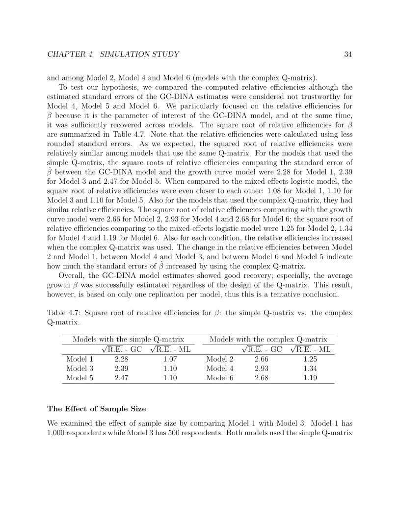
CHAPTER 4. SIMULATION STUDY 34
and among Model 2, Model 4 and Model 6 (models with the complex Q-matrix).To test our hypothesis, we compared the computed relative efficiencies although the
estimated standard errors of the GC-DINA estimates were considered not trustworthy forModel 4, Model 5 and Model 6. We particularly focused on the relative efficiencies forβ because it is the parameter of interest of the GC-DINA model, and at the same time,it was sufficiently recovered across models. The square root of relative efficiencies for βare summarized in Table 4.7. Note that the relative efficiencies were calculated using lessrounded standard errors. As we expected, the squared root of relative efficiencies wererelatively similar among models that use the same Q-matrix. For the models that used thesimple Q-matrix, the square roots of relative efficiencies comparing the standard error ofβ between the GC-DINA model and the growth curve model were 2.28 for Model 1, 2.39for Model 3 and 2.47 for Model 5. When compared to the mixed-effects logistic model, thesquare root of relative efficiencies were even closer to each other: 1.08 for Model 1, 1.10 forModel 3 and 1.10 for Model 5. Also for the models that used the complex Q-matrix, they hadsimilar relative efficiencies. The square root of relative efficiencies comparing with the growthcurve model were 2.66 for Model 2, 2.93 for Model 4 and 2.68 for Model 6; the square root ofrelative efficiencies comparing to the mixed-effects logistic model were 1.25 for Model 2, 1.34for Model 4 and 1.19 for Model 6. Also for each condition, the relative efficiencies increasedwhen the complex Q-matrix was used. The change in the relative efficiencies between Model2 and Model 1, between Model 4 and Model 3, and between Model 6 and Model 5 indicatehow much the standard errors of β increased by using the complex Q-matrix.
Overall, the GC-DINA model estimates showed good recovery; especially, the averagegrowth β was successfully estimated regardless of the design of the Q-matrix. This result,however, is based on only one replication per model, thus this is a tentative conclusion.
Table 4.7: Square root of relative efficiencies for β: the simple Q-matrix vs. the complexQ-matrix.
Models with the simple Q-matrix Models with the complex Q-matrix√R.E. - GC
√R.E. - ML
√R.E. - GC
√R.E. - ML
Model 1 2.28 1.07 Model 2 2.66 1.25Model 3 2.39 1.10 Model 4 2.93 1.34Model 5 2.47 1.10 Model 6 2.68 1.19
The Effect of Sample Size
We examined the effect of sample size by comparing Model 1 with Model 3. Model 1 has1,000 respondents while Model 3 has 500 respondents. Both models used the simple Q-matrix
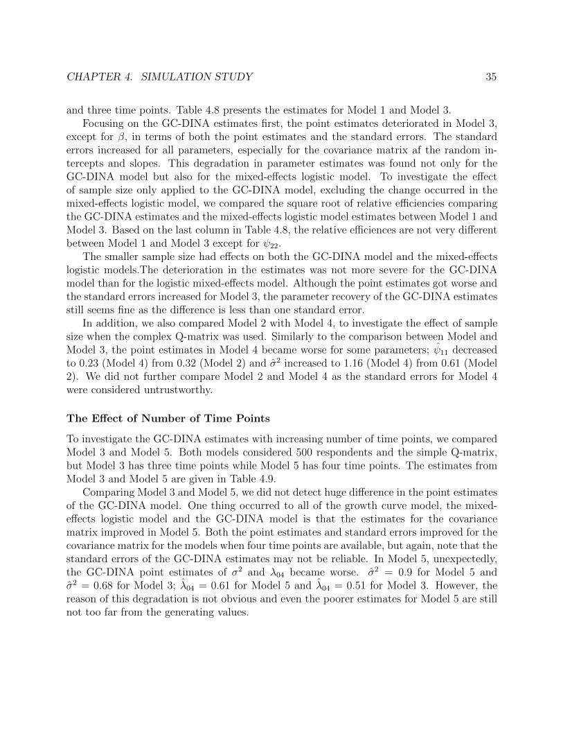
CHAPTER 4. SIMULATION STUDY 35
and three time points. Table 4.8 presents the estimates for Model 1 and Model 3.Focusing on the GC-DINA estimates first, the point estimates deteriorated in Model 3,
except for β, in terms of both the point estimates and the standard errors. The standarderrors increased for all parameters, especially for the covariance matrix af the random in-tercepts and slopes. This degradation in parameter estimates was found not only for theGC-DINA model but also for the mixed-effects logistic model. To investigate the effectof sample size only applied to the GC-DINA model, excluding the change occurred in themixed-effects logistic model, we compared the square root of relative efficiencies comparingthe GC-DINA estimates and the mixed-effects logistic model estimates between Model 1 andModel 3. Based on the last column in Table 4.8, the relative efficiences are not very differentbetween Model 1 and Model 3 except for ψ22.
The smaller sample size had effects on both the GC-DINA model and the mixed-effectslogistic models.The deterioration in the estimates was not more severe for the GC-DINAmodel than for the logistic mixed-effects model. Although the point estimates got worse andthe standard errors increased for Model 3, the parameter recovery of the GC-DINA estimatesstill seems fine as the difference is less than one standard error.
In addition, we also compared Model 2 with Model 4, to investigate the effect of samplesize when the complex Q-matrix was used. Similarly to the comparison between Model andModel 3, the point estimates in Model 4 became worse for some parameters; ψ11 decreasedto 0.23 (Model 4) from 0.32 (Model 2) and σ2 increased to 1.16 (Model 4) from 0.61 (Model2). We did not further compare Model 2 and Model 4 as the standard errors for Model 4were considered untrustworthy.
The Effect of Number of Time Points
To investigate the GC-DINA estimates with increasing number of time points, we comparedModel 3 and Model 5. Both models considered 500 respondents and the simple Q-matrix,but Model 3 has three time points while Model 5 has four time points. The estimates fromModel 3 and Model 5 are given in Table 4.9.
Comparing Model 3 and Model 5, we did not detect huge difference in the point estimatesof the GC-DINA model. One thing occurred to all of the growth curve model, the mixed-effects logistic model and the GC-DINA model is that the estimates for the covariancematrix improved in Model 5. Both the point estimates and standard errors improved for thecovariance matrix for the models when four time points are available, but again, note that thestandard errors of the GC-DINA estimates may not be reliable. In Model 5, unexpectedly,the GC-DINA point estimates of σ2 and λ04 became worse. σ2 = 0.9 for Model 5 andσ2 = 0.68 for Model 3; λ04 = 0.61 for Model 5 and λ04 = 0.51 for Model 3. However, thereason of this degradation is not obvious and even the poorer estimates for Model 5 are stillnot too far from the generating values.
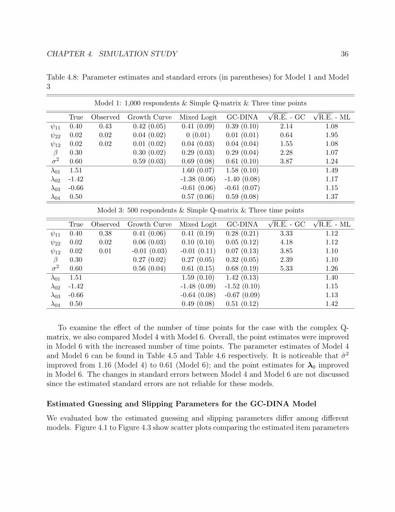
CHAPTER 4. SIMULATION STUDY 36
Table 4.8: Parameter estimates and standard errors (in parentheses) for Model 1 and Model3
Model 1: 1,000 respondents & Simple Q-matrix & Three time points
True Observed Growth Curve Mixed Logit GC-DINA√
R.E. - GC√
R.E. - ML
ψ11 0.40 0.43 0.42 (0.05) 0.41 (0.09) 0.39 (0.10) 2.14 1.08ψ22 0.02 0.02 0.04 (0.02) 0 (0.01) 0.01 (0.01) 0.64 1.95ψ12 0.02 0.02 0.01 (0.02) 0.04 (0.03) 0.04 (0.04) 1.55 1.08β 0.30 0.30 (0.02) 0.29 (0.03) 0.29 (0.04) 2.28 1.07σ2 0.60 0.59 (0.03) 0.69 (0.08) 0.61 (0.10) 3.87 1.24
λ01 1.51 1.60 (0.07) 1.58 (0.10) 1.49λ02 -1.42 -1.38 (0.06) -1.40 (0.08) 1.17λ03 -0.66 -0.61 (0.06) -0.61 (0.07) 1.15λ04 0.50 0.57 (0.06) 0.59 (0.08) 1.37
Model 3: 500 respondents & Simple Q-matrix & Three time points
True Observed Growth Curve Mixed Logit GC-DINA√
R.E. - GC√
R.E. - ML
ψ11 0.40 0.38 0.41 (0.06) 0.41 (0.19) 0.28 (0.21) 3.33 1.12ψ22 0.02 0.02 0.06 (0.03) 0.10 (0.10) 0.05 (0.12) 4.18 1.12ψ12 0.02 0.01 -0.01 (0.03) -0.01 (0.11) 0.07 (0.13) 3.85 1.10β 0.30 0.27 (0.02) 0.27 (0.05) 0.32 (0.05) 2.39 1.10σ2 0.60 0.56 (0.04) 0.61 (0.15) 0.68 (0.19) 5.33 1.26
λ01 1.51 1.59 (0.10) 1.42 (0.13) 1.40λ02 -1.42 -1.48 (0.09) -1.52 (0.10) 1.15λ03 -0.66 -0.64 (0.08) -0.67 (0.09) 1.13λ04 0.50 0.49 (0.08) 0.51 (0.12) 1.42
To examine the effect of the number of time points for the case with the complex Q-matrix, we also compared Model 4 with Model 6. Overall, the point estimates were improvedin Model 6 with the increased number of time points. The parameter estimates of Model 4and Model 6 can be found in Table 4.5 and Table 4.6 respectively. It is noticeable that σ2
improved from 1.16 (Model 4) to 0.61 (Model 6); and the point estimates for λ0 improvedin Model 6. The changes in standard errors between Model 4 and Model 6 are not discussedsince the estimated standard errors are not reliable for these models.
Estimated Guessing and Slipping Parameters for the GC-DINA Model
We evaluated how the estimated guessing and slipping parameters differ among differentmodels. Figure 4.1 to Figure 4.3 show scatter plots comparing the estimated item parameters
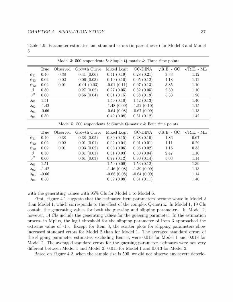
CHAPTER 4. SIMULATION STUDY 37
Table 4.9: Parameter estimates and standard errors (in parentheses) for Model 3 and Model5
Model 3: 500 respondents & Simple Q-matrix & Three time points
True Observed Growth Curve Mixed Logit GC-DINA√
R.E. - GC√
R.E. - ML
ψ11 0.40 0.38 0.41 (0.06) 0.41 (0.19) 0.28 (0.21) 3.33 1.12ψ22 0.02 0.02 0.06 (0.03) 0.10 (0.10) 0.05 (0.12) 4.18 1.12ψ12 0.02 0.01 -0.01 (0.03) -0.01 (0.11) 0.07 (0.13) 3.85 1.10β 0.30 0.27 (0.02) 0.27 (0.05) 0.32 (0.05) 2.39 1.10σ2 0.60 0.56 (0.04) 0.61 (0.15) 0.68 (0.19) 5.33 1.26
λ01 1.51 1.59 (0.10) 1.42 (0.13) 1.40λ02 -1.42 -1.48 (0.09) -1.52 (0.10) 1.15λ03 -0.66 -0.64 (0.08) -0.67 (0.09) 1.13λ04 0.50 0.49 (0.08) 0.51 (0.12) 1.42
Model 5: 500 respondents & Simple Q-matrix & Four time points
True Observed Growth Curve Mixed Logit GC-DINA√
R.E. - GC√
R.E. - ML
ψ11 0.40 0.38 0.38 (0.05) 0.39 (0.15) 0.28 (0.10) 1.86 0.67ψ22 0.02 0.02 0.01 (0.01) 0.02 (0.04) 0.01 (0.01) 1.11 0.29ψ12 0.02 0.01 0.03 (0.02) 0.03 (0.06) 0.06 (0.02) 1.16 0.33β 0.30 0.31 (0.01) 0.31 (0.03) 0.30 (0.04) 2.47 1.10σ2 0.60 0.61 (0.03) 0.77 (0.12) 0.90 (0.14) 5.03 1.14
λ01 1.51 1.59 (0.09) 1.53 (0.12) 1.39λ02 -1.42 -1.46 (0.08) -1.39 (0.09) 1.13λ03 -0.66 -0.68 (0.08) -0.64 (0.09) 1.14λ04 0.50 0.52 (0.08) 0.61 (0.11) 1.40
with the generating values with 95% CIs for Model 1 to Model 6.First, Figure 4.1 suggests that the estimated item parameters became worse in Model 2
than Model 1, which corresponds to the effect of the complex Q-matrix. In Model 1, 19 CIscontain the generating values for both the guessing and slipping parameters. In Model 2,however, 14 CIs include the generating values for the guessing parameter. In the estimationprocess in Mplus, the logit threshold for the slipping parameter of Item 3 approached theextreme value of -15. Except for Item 3, the scatter plots for slipping parameters showincreased standard errors for Model 2 than for Model 1. The averaged standard errors ofthe slipping parameter estimates, excluding Item 3, were 0.013 for Model 1 and 0.018 forModel 2. The averaged standard errors for the guessing parameter estimates were not verydifferent between Model 1 and Model 2: 0.015 for Model 1 and 0.013 for Model 2.
Based on Figure 4.2, when the sample size is 500, we did not observe any severe deterio-

CHAPTER 4. SIMULATION STUDY 38
ration due to the complex Q-matrix. Model 4 shows increased length of error bars especiallyfor the slipping parameter estimates–the averaged standard errors of the slipping parameterestimates were 0.018 for Model 3 and 0.023 for Model 4, but the errors in Model 4 may not betrustworthy. When comparing Model 5 and Model 6 for the four time points, there was notsignificant effects of the complex Q-matrix on the estimated item parameters. The guessingand slipping parameter estimates were not very different between Model 5 and Model 6, andshowed overall good recovery.
Comparing Model 1 and Model 3, to examine the effect of sample size, it is noticeablethat standard errors increased for Model 3 than for Model 1—the averaged standard errorsfor the estimated guessing parameters were 0.015 for Model 1 and 0.021 for Model 3 and theaveraged errors for the estimated slipping parameters were 0.013 for Model 1 and 0.018 forModel 3. The point estimates, however, did not deteriorate with the smaller sample size.
We then compared Model 3 and Model 5 to investigate changes in the item parameterestimates depending on the number of time points. For both models, the estimated itemparameters and the generating values were both close to each other. It appeared the GC-DINA estimates recovered the generating values well enough in both cases with three andfour time points.
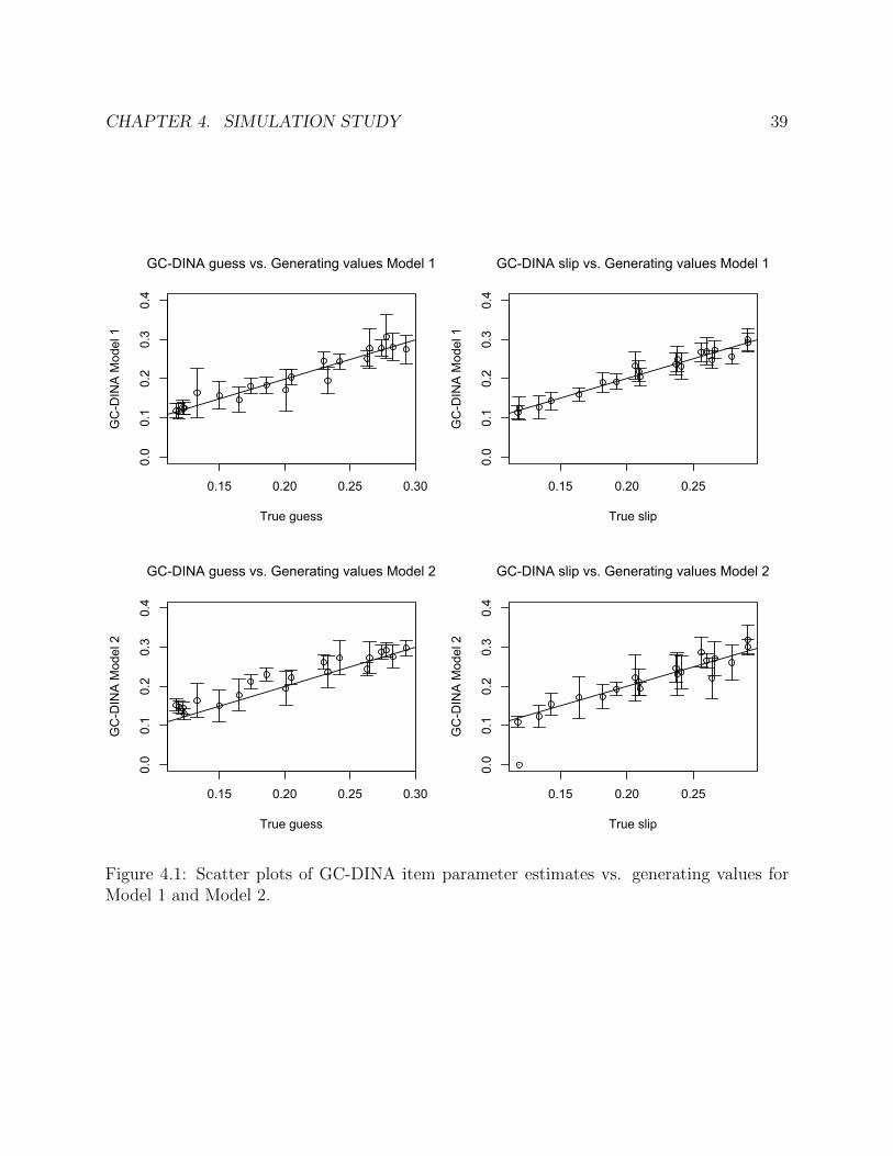
CHAPTER 4. SIMULATION STUDY 39
0.15 0.20 0.25 0.30
0.0
0.1
0.2
0.3
0.4
True guess
GC
-DIN
A M
odel
1
GC-DINA guess vs. Generating values Model 1
0.15 0.20 0.250.0
0.1
0.2
0.3
0.4
True slip
GC
-DIN
A M
odel
1
GC-DINA slip vs. Generating values Model 1
0.15 0.20 0.25 0.30
0.0
0.1
0.2
0.3
0.4
True guess
GC
-DIN
A M
odel
2
GC-DINA guess vs. Generating values Model 2
0.15 0.20 0.25
0.0
0.1
0.2
0.3
0.4
True slip
GC
-DIN
A M
odel
2
GC-DINA slip vs. Generating values Model 2
Figure 4.1: Scatter plots of GC-DINA item parameter estimates vs. generating values forModel 1 and Model 2.
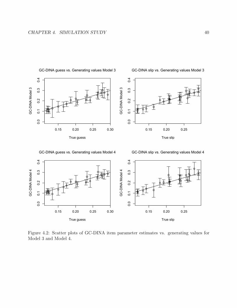
CHAPTER 4. SIMULATION STUDY 40
0.15 0.20 0.25 0.30
0.0
0.1
0.2
0.3
0.4
True guess
GC
-DIN
A M
odel
3
GC-DINA guess vs. Generating values Model 3
0.15 0.20 0.250.0
0.1
0.2
0.3
0.4
True slip
GC
-DIN
A M
odel
3
GC-DINA slip vs. Generating values Model 3
0.15 0.20 0.25 0.30
0.0
0.1
0.2
0.3
0.4
True guess
GC
-DIN
A M
odel
4
GC-DINA guess vs. Generating values Model 4
0.15 0.20 0.25
0.0
0.1
0.2
0.3
0.4
True slip
GC
-DIN
A M
odel
4
GC-DINA slip vs. Generating values Model 4
Figure 4.2: Scatter plots of GC-DINA item parameter estimates vs. generating values forModel 3 and Model 4.
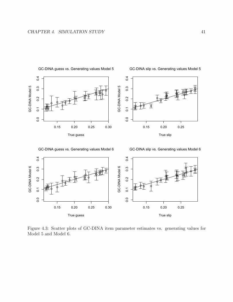
CHAPTER 4. SIMULATION STUDY 41
0.15 0.20 0.25 0.30
0.0
0.1
0.2
0.3
0.4
True guess
GC
-DIN
A M
odel
5
GC-DINA guess vs. Generating values Model 5
0.15 0.20 0.250.0
0.1
0.2
0.3
0.4
True slip
GC
-DIN
A M
odel
5
GC-DINA slip vs. Generating values Model 5
0.15 0.20 0.25 0.30
0.0
0.1
0.2
0.3
0.4
True guess
GC
-DIN
A M
odel
6
GC-DINA guess vs. Generating values Model 6
0.15 0.20 0.25
0.0
0.1
0.2
0.3
0.4
True slip
GC
-DIN
A M
odel
6
GC-DINA slip vs. Generating values Model 6
Figure 4.3: Scatter plots of GC-DINA item parameter estimates vs. generating values forModel 5 and Model 6.
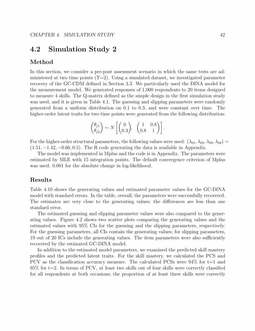
CHAPTER 4. SIMULATION STUDY 42
4.2 Simulation Study 2
Method
In this section, we consider a pre-post assessment scenario in which the same tests are ad-ministered at two time points (T=2). Using a simulated dataset, we investigated parameterrecovery of the GC-CDM defined in Section 3.3. We particularly used the DINA model forthe measurement model. We generated responses of 1,000 respondents to 20 items designedto measure 4 skills. The Q-matrix defined as the simple design in the first simulation studywas used, and it is given in Table 4.1. The guessing and slipping parameters were randomlygenerated from a uniform distribution on 0.1 to 0.3, and were constant over time. Thehigher-order latent traits for two time points were generated from the following distribution:(
θj1θj2
)∼ N
[(0
0.3
),
(1 0.8
0.8 1
)].
For the higher-order structural parameters, the following values were used: (λ01, λ02, λ03, λ04) =(1.51,−1.42,−0.66, 0.5). The R code generating the data is available in Appendix.
The model was implemented in Mplus and the code is in Appendix. The parameters wereestimated by MLE with 15 integration points. The default convergence criterion of Mpluswas used: 0.001 for the absolute change in log-likelihood.
Results
Table 4.10 shows the generating values and estimated parameter values for the GC-DINAmodel with standard errors. In the table, overall, the parameters were successfully recovered.The estimates are very close to the generating values; the differences are less than onestandard error.
The estimated guessing and slipping parameter values were also compared to the gener-ating values. Figure 4.2 shows two scatter plots comparing the generating values and theestimated values with 95% CIs for the guessing and the slipping parameters, respectively.For the guessing parameters, all CIs contain the generating values; for slipping parameters,19 out of 20 ICs include the generating values. The item parameters were also sufficientlyrecovered by the estimated GC-DINA model.
In addition to the estimated model parameters, we examined the predicted skill masteryprofiles and the predicted latent traits. For the skill mastery, we calculated the PCS andPCV as the classification accuracy measure. The calculated PCSs were 94% for t=1 and95% for t=2. In terms of PCV, at least two skills out of four skills were correctly classifiedfor all respondents at both occasions; the proportion of at least three skills were correctly
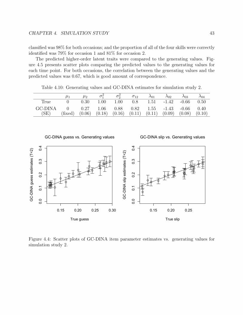
CHAPTER 4. SIMULATION STUDY 43
classified was 98% for both occasions; and the proportion of all of the four skills were correctlyidentified was 79% for occasion 1 and 81% for occasion 2.
The predicted higher-order latent traits were compared to the generating values. Fig-ure 4.5 presents scatter plots comparing the predicted values to the generating values foreach time point. For both occasions, the correlation between the generating values and thepredicted values was 0.67, which is good amount of correspondence.
Table 4.10: Generating values and GC-DINA estimates for simulation study 2.
µ1 µ2 σ21 σ2
2 σ12 λ01 λ02 λ03 λ04True 0 0.30 1.00 1.00 0.8 1.51 -1.42 -0.66 0.50
GC-DINA 0 0.27 1.06 0.88 0.82 1.55 -1.43 -0.66 0.40(SE) (fixed) (0.06) (0.18) (0.16) (0.11) (0.11) (0.09) (0.08) (0.10)
0.15 0.20 0.25 0.30
0.0
0.1
0.2
0.3
0.4
True guess
GC
-DIN
A g
uess
est
imat
es (T
=2)
GC-DINA guess vs. Generating values
0.15 0.20 0.25
0.0
0.1
0.2
0.3
0.4
True slip
GC
-DIN
A s
lip e
stim
ates
(T=2
)
GC-DINA slip vs. Generating values
Figure 4.4: Scatter plots of GC-DINA item parameter estimates vs. generating values forsimulation study 2.

CHAPTER 4. SIMULATION STUDY 44
-3 -2 -1 0 1 2 3
-1.5
-0.5
0.5
1.5
Generating values
GC
-DIN
A e
stim
ates
GC-DINA vs. Generating values at t=1 (r=0.67)
-3 -2 -1 0 1 2 3
-1.0
0.0
0.5
1.0
1.5
Generating values
GC
-DIN
A e
stim
ates
GC-DINA vs. Generating values at t=2 (r=0.67)
Figure 4.5: Scatter plots of predicted higher-order latent traits from the GC-DINA modelvs. generating values for simulation study 2. The estimated correlation, r, is in parenthesis.
45
Chapter 5
Empirical Study
In this chapter, we use two examples to illustrate application of the GC-DINA model. Thedata sets are from multi-wave experiments designed to assess the effects of an instructionaltreatment called Enhanced Anchored Instruction (EAI; Bottge et al., 2003) on mathematicsachievement of middle school students with learning disabilities (LD) and without learningdisabilities (NLD).
5.1 Fraction of the Cost (FOC) test data
Data
A study was designed to assess the effects of two different EAI instructions: Kim’s Koment(KK) and Fraction of the Cost (FOC) (Bottge et al., 2007). The KK instruction had theprimary goal to guide students to develop informal understanding of pre-algebraic concepts,including linear function, line of best fit, variables, rate of change (slope), and reliabilityand measurement error. KK includes video instruction depicting two girls competing inpentathlon events. Here, with instruction from the video anchor, students learn to identifythe fastest cars in the race, based on times and distances and also learn to construct the “lineof best fit” to predict the speed of the cars when released from various points on the ramp.The FOC, on the other hand, depicts three middle school students trying to buy materialsfor a skateboard ramp. The aim is that students learn various concepts and skills and applythem holistically to solve a problem. The skills include (a) calculate the percent of moneyin a savings account and sales tax on a purchase, (b) read a tape measure, (c) convert feetto inches, (d) decipher building plans, (e) construct a table of materials, (f) compute wholenumbers and mixed fractions, (g) estimate and compute combinations, and (h) calculatetotal cost.
CHAPTER 5. EMPIRICAL STUDY 46
For the study, 109 students were selected from six math classrooms in a school districtin a small upper Midwestern town. The sample consisted of 50 males and 59 females in theseventh grade. 9 students were with LD and the remainder of the students were NLD. TheKK and FOC instructions were administered during the academic year as follows: betweenWeek 1 and 4, the KK instruction was taught for 13 days; between Week 4 and 19, theregular math curriculum was taught; and between Week 19 and 24, the FOC instructionwas administered. In the regular instruction, teachers taught units on concepts related togeometry and proportional reasoning.
The FOC test, which is designed to assess the effects of the FOC instruction, was ad-ministered at four time points, at Weeks 1, 4, 19 and 24, before and after each of the threeinstructional sequences. The FOC test consists of 23 items that measure four skills. TheQ-matrix for the FOC test is given in Table 5.1. This Q-matrix, apart from the rows foritems 11, 12, and 13, was used as the complex Q-matrix for the simulation study in Section4.1.
Results
The GC-DINA model was fitted to the FOC test data using Mplus. The parameters wereestimated with 15 integration points, the convergence criterion of 10−7 for the absolutechange in the log-likelihood and the maximum number of EM iterations was 1,000. Notethat the default for the number of EM iterations is 500 in Mplus, but the estimation did notconverge within 500 iterations.
The estimated parameters are given in Table 5.2. The variance of the person-specificrandom intercept was estimated as 7.20 which implies large variation between students intheir overall higher-order latent traits. This also means that skill mastery is highly correlatedacross skills; the estimated intraclass correlation of the latent responses for skill mastery is0.60. The correlation between the random intercept and the random slope of time is closeto -1. This negative relationship corresponds to the idea that the EAI treatments weredeveloped to be effective for students with LD. Thus, the low achieving students might havebenefited more from the EAI than high achieving students.
The estimated average growth, β = 1.81, suggests that students’ overall abilities improvedover time on average. The corresponding odds-ratio of 6.1 means that, for a median student(with random slope equal to the median of 0), the odds of mastering each skill increases by afactor of six between testing occasions. Figure 5.1 displays the predicted higher-order latenttraits over time, which were calculated by θjt = ζ1j + (β+ ζ2j)× timet + εjt. It shows that allstudents’ overall mathematics abilities were predicted to improve over the four time points.
The FOC test data were also analyzed by Li et al. (2016) using the LTA-DINA model. Wecompared the estimated item parameter values from the GC-DINA model with the LTA-DINA estimates reported in their paper. Figure 5.2 presents scatter plots comparing the
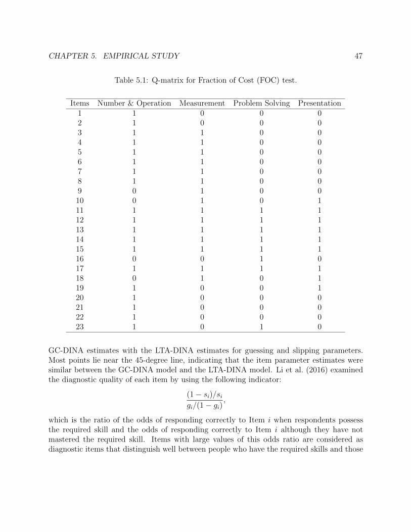
CHAPTER 5. EMPIRICAL STUDY 47
Table 5.1: Q-matrix for Fraction of Cost (FOC) test.
Items Number & Operation Measurement Problem Solving Presentation1 1 0 0 02 1 0 0 03 1 1 0 04 1 1 0 05 1 1 0 06 1 1 0 07 1 1 0 08 1 1 0 09 0 1 0 010 0 1 0 111 1 1 1 112 1 1 1 113 1 1 1 114 1 1 1 115 1 1 1 116 0 0 1 017 1 1 1 118 0 1 0 119 1 0 0 120 1 0 0 021 1 0 0 022 1 0 0 023 1 0 1 0
GC-DINA estimates with the LTA-DINA estimates for guessing and slipping parameters.Most points lie near the 45-degree line, indicating that the item parameter estimates weresimilar between the GC-DINA model and the LTA-DINA model. Li et al. (2016) examinedthe diagnostic quality of each item by using the following indicator:
(1− si)/sigi/(1− gi)
,
which is the ratio of the odds of responding correctly to Item i when respondents possessthe required skill and the odds of responding correctly to Item i although they have notmastered the required skill. Items with large values of this odds ratio are considered asdiagnostic items that distinguish well between people who have the required skills and those
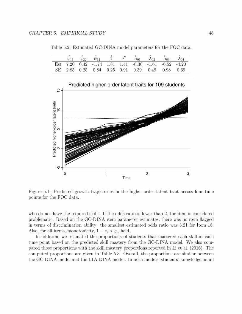
CHAPTER 5. EMPIRICAL STUDY 48
Table 5.2: Estimated GC-DINA model parameters for the FOC data.
ψ11 ψ22 ψ12 β σ2 λ01 λ02 λ03 λ04Est 7.20 0.42 -1.74 1.81 1.41 -0.30 -1.61 -6.52 -4.20SE 2.85 0.25 0.84 0.25 0.91 0.39 0.49 0.98 0.69
-50
510
15Pr
edic
ted
high
er-o
rder
late
nt tr
aits
0 1 2 3Time
Predicted higher-order latent traits for 109 students
Figure 5.1: Predicted growth trajectories in the higher-order latent trait across four timepoints for the FOC data.
who do not have the required skills. If the odds ratio is lower than 2, the item is consideredproblematic. Based on the GC-DINA item parameter estimates, there was no item flaggedin terms of discrimination ability: the smallest estimated odds ratio was 3.21 for Item 18.Also, for all items, monotonicity, 1− si > gi, held.
In addition, we estimated the proportions of students that mastered each skill at eachtime point based on the predicted skill mastery from the GC-DINA model. We also com-pared those proportions with the skill mastery proportions reported in Li et al. (2016). Thecomputed proportions are given in Table 5.3. Overall, the proportions are similar betweenthe GC-DINA model and the LTA-DINA model. In both models, students’ knowledge on all
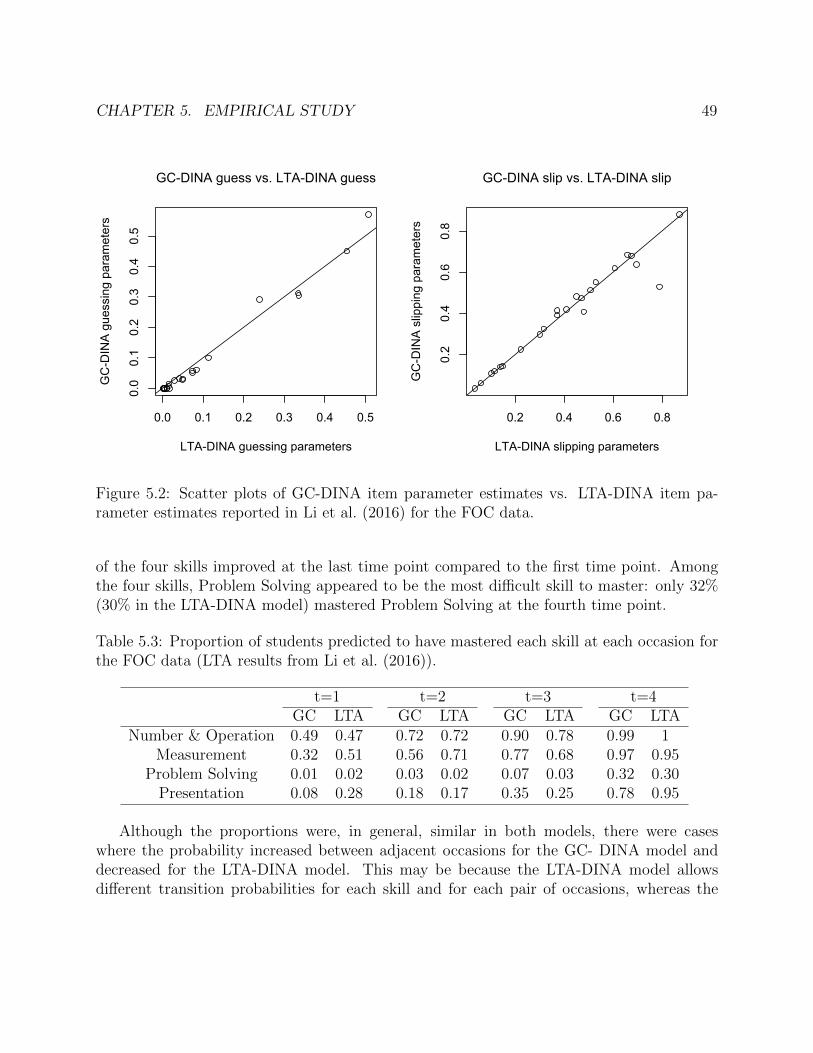
CHAPTER 5. EMPIRICAL STUDY 49
0.0 0.1 0.2 0.3 0.4 0.5
0.0
0.1
0.2
0.3
0.4
0.5
LTA-DINA guessing parameters
GC
-DIN
A g
uess
ing
para
met
ers
GC-DINA guess vs. LTA-DINA guess
0.2 0.4 0.6 0.8
0.2
0.4
0.6
0.8
LTA-DINA slipping parameters
GC
-DIN
A s
lippi
ng p
aram
eter
s
GC-DINA slip vs. LTA-DINA slip
Figure 5.2: Scatter plots of GC-DINA item parameter estimates vs. LTA-DINA item pa-rameter estimates reported in Li et al. (2016) for the FOC data.
of the four skills improved at the last time point compared to the first time point. Amongthe four skills, Problem Solving appeared to be the most difficult skill to master: only 32%(30% in the LTA-DINA model) mastered Problem Solving at the fourth time point.
Table 5.3: Proportion of students predicted to have mastered each skill at each occasion forthe FOC data (LTA results from Li et al. (2016)).
t=1 t=2 t=3 t=4GC LTA GC LTA GC LTA GC LTA
Number & Operation 0.49 0.47 0.72 0.72 0.90 0.78 0.99 1Measurement 0.32 0.51 0.56 0.71 0.77 0.68 0.97 0.95
Problem Solving 0.01 0.02 0.03 0.02 0.07 0.03 0.32 0.30Presentation 0.08 0.28 0.18 0.17 0.35 0.25 0.78 0.95
Although the proportions were, in general, similar in both models, there were caseswhere the probability increased between adjacent occasions for the GC- DINA model anddecreased for the LTA-DINA model. This may be because the LTA-DINA model allowsdifferent transition probabilities for each skill and for each pair of occasions, whereas the
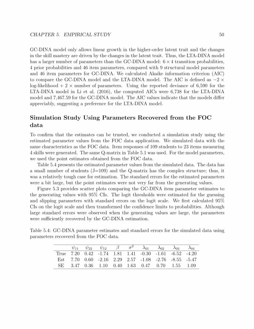
CHAPTER 5. EMPIRICAL STUDY 50
GC-DINA model only allows linear growth in the higher-order latent trait and the changesin the skill mastery are driven by the changes in the latent trait. Thus, the LTA-DINA modelhas a larger number of parameters than the GC-DINA model: 6× 4 transition probabilities,4 prior probabilities and 46 item parameters, compared with 9 structural model parametersand 46 item parameters for GC-DINA. We calculated Akaike information criterion (AIC)to compare the GC-DINA model and the LTA-DINA model. The AIC is defined as −2 ×log-likelihood + 2 × number of parameters. Using the reported deviance of 6,590 for theLTA-DINA model in Li et al. (2016), the computed AICs were 6,738 for the LTA-DINAmodel and 7,467.59 for the GC-DINA model. The AIC values indicate that the models differappreciably, suggesting a preference for the LTA-DINA model.
Simulation Study Using Parameters Recovered from the FOCdata
To confirm that the estimates can be trusted, we conducted a simulation study using theestimated parameter values from the FOC data application. We simulated data with thesame characteristics as the FOC data. Item responses of 109 students to 23 items measuring4 skills were generated. The same Q-matrix in Table 5.1 was used. For the model parameters,we used the point estimates obtained from the FOC data.
Table 5.4 presents the estimated parameter values from the simulated data. The data hasa small number of students (J=109) and the Q-matrix has the complex structure; thus, itwas a relatively tough case for estimation. The standard errors for the estimated parameterswere a bit large, but the point estimates were not very far from the generating values.
Figure 5.3 provides scatter plots comparing the GC-DINA item parameter estimates tothe generating values with 95% CIs. The logit thresholds were estimated for the guessingand slipping parameters with standard errors on the logit scale. We first calculated 95%CIs on the logit scale and then transformed the confidence limits to probabilities. Althoughlarge standard errors were observed when the generating values are large, the parameterswere sufficiently recovered by the GC-DINA estimation.
Table 5.4: GC-DINA parameter estimates and standard errors for the simulated data usingparameters recovered from the FOC data.
ψ11 ψ22 ψ12 β σ2 λ01 λ02 λ03 λ04True 7.20 0.42 -1.74 1.81 1.41 -0.30 -1.61 -6.52 -4.20Est 7.70 0.60 -2.16 2.29 2.57 -1.08 -2.76 -8.55 -5.47SE 3.47 0.36 1.10 0.40 1.63 0.47 0.70 1.55 1.09

CHAPTER 5. EMPIRICAL STUDY 51
0.0 0.1 0.2 0.3 0.4 0.5
0.0
0.2
0.4
0.6
0.8
1.0
True guess
GC
-DIN
A e
stim
ates
GC-DINA guess vs. Generating values
0.2 0.4 0.6 0.8
0.0
0.2
0.4
0.6
0.8
1.0
True slip
GC
-DIN
A e
stim
ates
GC-DINA slip vs. Generating values
Figure 5.3: Scatter plots of GC-DINA item parameter estimates vs. generating values forthe simulated data using parameters recovered from the FOC data.
5.2 Problem Solving Test (PST) data
Data
The second dataset was obtained from a pre-post test cluster-randomized trial designed toestimate the effects of combining explicit and anchored instruction on fraction computationand problem solving. The experiment considered two instructional conditions: EAI andbusiness as usual (BAU), and random assignment was conducted at the school level. EAIinstruction includes five EAI units: KK, FOC, Fractions at Work (FAW), Hovercraft Project(HOV), and Grand Pentathlon (GP). Teachers assigned to the BAU condition followed theirregular school math curriculum. To examine the effects of the EAI on students computationand problem solving skills, two researcher-developed tests (Fractions Computation Test,Problem-Solving Test) and two standardized achievement tests (two math sub-tests of theITBS) were administered prior to and following the instructional period.
We analyzed students’ responses of the Problem-Solving Test (PST). The test consistsof 21 items measuring “Ratios and Proportional Relationships”, “Measurement and Data”,“Number and Operations-Fractions”, “Geometry” and “Statistics and Probability”. TheQ-matrix was developed with the simple structure where all items measure a single skill.
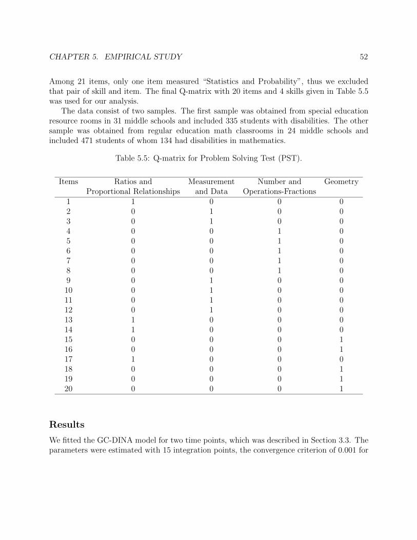
CHAPTER 5. EMPIRICAL STUDY 52
Among 21 items, only one item measured “Statistics and Probability”, thus we excludedthat pair of skill and item. The final Q-matrix with 20 items and 4 skills given in Table 5.5was used for our analysis.
The data consist of two samples. The first sample was obtained from special educationresource rooms in 31 middle schools and included 335 students with disabilities. The othersample was obtained from regular education math classrooms in 24 middle schools andincluded 471 students of whom 134 had disabilities in mathematics.
Table 5.5: Q-matrix for Problem Solving Test (PST).
Items Ratios and Measurement Number and GeometryProportional Relationships and Data Operations-Fractions
1 1 0 0 02 0 1 0 03 0 1 0 04 0 0 1 05 0 0 1 06 0 0 1 07 0 0 1 08 0 0 1 09 0 1 0 010 0 1 0 011 0 1 0 012 0 1 0 013 1 0 0 014 1 0 0 015 0 0 0 116 0 0 0 117 1 0 0 018 0 0 0 119 0 0 0 120 0 0 0 1
Results
We fitted the GC-DINA model for two time points, which was described in Section 3.3. Theparameters were estimated with 15 integration points, the convergence criterion of 0.001 for
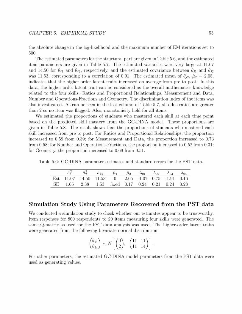
CHAPTER 5. EMPIRICAL STUDY 53
the absolute change in the log-likelihood and the maximum number of EM iterations set to500.
The estimated parameters for the structural part are given in Table 5.6, and the estimateditem parameters are given in Table 5.7. The estimated variances were very large at 11.07and 14.50 for θj1 and θj2, respectively, and the estimated covariance between θj1 and θj2was 11.53, corresponding to a correlation of 0.91. The estimated mean of θj2, µ2 = 2.05,indicates that the higher-order latent traits increased on average from pre to post. In thisdata, the higher-order latent trait can be considered as the overall mathematics knowledgerelated to the four skills: Ratios and Proportional Relationships, Measurement and Data,Number and Operations-Fractions and Geometry. The discrimination index of the items wasalso investigated. As can be seen in the last column of Table 5.7, all odds ratios are greaterthan 2 so no item was flagged. Also, monotonicity held for all items.
We estimated the proportions of students who mastered each skill at each time pointbased on the predicted skill mastery from the GC-DINA model. These proportions aregiven in Table 5.8. The result shows that the proportions of students who mastered eachskill increased from pre to post. For Ratios and Proportional Relationships, the proportionincreased to 0.59 from 0.39; for Measurement and Data, the proportion increased to 0.73from 0.58; for Number and Operations-Fractions, the proportion increased to 0.52 from 0.31;for Geometry, the proportion increased to 0.69 from 0.51.
Table 5.6: GC-DINA parameter estimates and standard errors for the PST data.
σ21 σ2
2 σ12 µ1 µ2 λ01 λ02 λ03 λ04Est 11.07 14.50 11.53 0 2.05 -1.07 0.75 -1.91 0.16SE 1.65 2.38 1.53 fixed 0.17 0.24 0.21 0.24 0.28
Simulation Study Using Parameters Recovered from the PST data
We conducted a simulation study to check whether our estimates appear to be trustworthy.Item responses for 800 respondents to 20 items measuring four skills were generated. Thesame Q-matrix as used for the PST data analysis was used. The higher-order latent traitswere generated from the following bivariate normal distribution:(
θ1jθ2j
)∼ N
[(02
),
(11 1111 14
)].
For other parameters, the estimated GC-DINA model parameters from the PST data wereused as generating values.
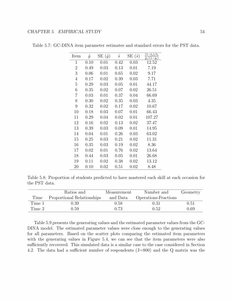
CHAPTER 5. EMPIRICAL STUDY 54
Table 5.7: GC-DINA item parameter estimates and standard errors for the PST data.
Item g SE (g) s SE (s) (1−si)/sigi/(1−gi)
1 0.10 0.01 0.42 0.03 12.522 0.49 0.03 0.13 0.01 7.193 0.06 0.01 0.65 0.02 9.174 0.17 0.02 0.39 0.03 7.715 0.29 0.03 0.05 0.01 44.176 0.35 0.02 0.07 0.02 26.517 0.03 0.01 0.37 0.04 66.698 0.30 0.02 0.35 0.03 4.359 0.32 0.02 0.17 0.02 10.6710 0.18 0.03 0.07 0.01 66.4311 0.29 0.04 0.02 0.01 107.2712 0.16 0.02 0.13 0.02 37.4713 0.39 0.03 0.09 0.01 14.9514 0.04 0.01 0.26 0.03 63.0215 0.25 0.03 0.21 0.02 11.3116 0.35 0.03 0.19 0.02 8.3617 0.02 0.01 0.76 0.02 13.6418 0.44 0.03 0.05 0.01 26.6819 0.11 0.02 0.38 0.02 13.1220 0.10 0.02 0.51 0.02 8.48
Table 5.8: Proportion of students predicted to have mastered each skill at each occasion forthe PST data.
Ratios and Measurement Number and GeometryTime Proportional Relationships and Data Operations-Fractions
Time 1 0.39 0.58 0.31 0.51Time 2 0.59 0.73 0.52 0.69
Table 5.9 presents the generating values and the estimated parameter values from the GC-DINA model. The estimated parameter values were close enough to the generating valuesfor all parameters. Based on the scatter plots comparing the estimated item parameterswith the generating values in Figure 5.4, we can see that the item parameters were alsosufficiently recovered. This simulated data is a similar case to the case considered in Section4.2. The data had a sufficient number of respondents (J=800) and the Q matrix was the
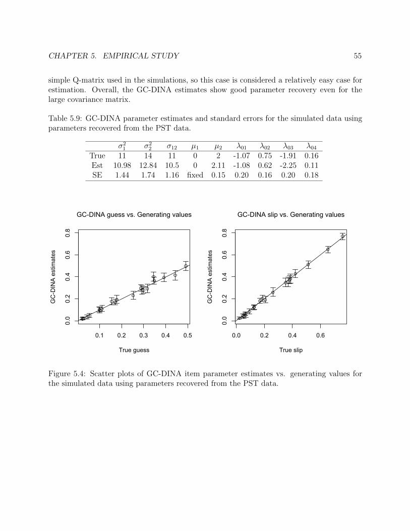
CHAPTER 5. EMPIRICAL STUDY 55
simple Q-matrix used in the simulations, so this case is considered a relatively easy case forestimation. Overall, the GC-DINA estimates show good parameter recovery even for thelarge covariance matrix.
Table 5.9: GC-DINA parameter estimates and standard errors for the simulated data usingparameters recovered from the PST data.
σ21 σ2
2 σ12 µ1 µ2 λ01 λ02 λ03 λ04True 11 14 11 0 2 -1.07 0.75 -1.91 0.16Est 10.98 12.84 10.5 0 2.11 -1.08 0.62 -2.25 0.11SE 1.44 1.74 1.16 fixed 0.15 0.20 0.16 0.20 0.18
0.1 0.2 0.3 0.4 0.5
0.0
0.2
0.4
0.6
0.8
True guess
GC
-DIN
A e
stim
ates
GC-DINA guess vs. Generating values
0.0 0.2 0.4 0.6
0.0
0.2
0.4
0.6
0.8
True slip
GC
-DIN
A e
stim
ates
GC-DINA slip vs. Generating values
Figure 5.4: Scatter plots of GC-DINA item parameter estimates vs. generating values forthe simulated data using parameters recovered from the PST data.
56
Chapter 6
Comparison of LongitudinalPsychometric Models
6.1 Introduction
This chapter considers different longitudinal psychometric models described in Chapter 2to examine their similarity when fitted to the same data. For simplicity and clarity, wefocus on the situation where there are two occasions, T = 2. We compare our GC-CDM tothe LTA-CDM (Li et al., 2016) and Andersen’s longitudinal IRT model (Andersen, 1985),henceforth referred to as the longitudinal Rasch model. The LTA-CDM and the longitudinalIRT model have similarities with the GC-CDM in that the LTA-CDM traces skill masteryover time and the longitudinal Rasch model measures growth in the latent trait.
Using a data set generated from the GC-DINA model, our study focuses on the followingresearch questions:
1. What are the parameter estimates of the GC-DINA, LTA-DINA and longitudinal IRTmodels?
2. How well do the models fit the data?
3. What are the predicted skill mastery profiles from the GC-DINA and the LTA-DINAand how do they differ?
4. What are the predicted latent traits from the GC-DINA and the longitudinal IRTmodel and how do they differ?
CHAPTER 6. COMPARISON OF LONGITUDINAL PSYCHOMETRIC MODELS 57
6.2 Method
For the simulation study, the same dataset generated for simulation study 2 in Chapter 4 wasused. We give a brief summary of data generation here. Item responses of 1,000 persons to20 items at 2 occasions were generated from the GC-DINA model. The assessment measuresfour skills with the simple Q-matrix in Table 4.1. The latent traits for the two occasionswere generated from the following bivariate normal distribution:(
θ1jθ2j
)∼ N
[(0
0.3
),
(1 0.8
0.8 1
)].
For the higher-order structural model, the Rasch model was used with the intercepts, λ0 =(1.51,−1.42,−0.66, 0.50)
′. The guessing and slipping parameters were randomly generated
from an uniform distribution from 0.1 to 0.3, and were constant over time.For the comparison, we considered the following models: the GC-DINA model described
in Section 3.3 with time-constant guessing and slipping parameters, the LTA-DINA modelwith different transition probabilities for each skill and time-constant guessing and slippingparameters, and the longitudinal Rasch model with a bivariate normal distribution of abilityand time-constant item difficulty parameters. The longitudianl IRT and GC-DINA modeltherefore both assumed a bivariate normal distribution for the latent traits because a fullgrowth-curve model is not identified with two occasions. All models were fitted in Mplus,and the codes for the LTA-DINA model and the longitudinal Rasch model are presented inAppendix.
6.3 Results
Parameter Estimates and Model Fit
The estimated model parameters from the GC-DINA, LTA-DINA and longitudinal Raschmodel are given in Tables 6.1 to 6.4. Table 6.1 shows the estimated mean and covariancematrix of θ for the GC-DINA and longitudinal Rasch models. The GC-DINA model esti-mates are close to the generating values whereas the estimates from the longitudinal Raschmodel differ a little. In particular, the longitudinal Rasch model gives a smaller varianceof 0.52 for θ1 and 0.49 of θ2 and a smaller mean of θ2 of 0.09. In Table 6.2, the GC-DINAmodel shows good parameter recovery for the higher-order structural parameters λ0.
Table 6.3 presents the estimated transition probabilities for the LTA-DINA model. pm1
indicates the probability of skill mastery at the first occasion; pm|n is the transition probabil-ity from non-mastery to mastery; pm|m is the transition probability from mastery to mastery;pn|m is the transition probability from mastery to non-mastery; pn|n is the transition prob-ability from non-mastery to non-mastery. The model implies that, for the first time point,
CHAPTER 6. COMPARISON OF LONGITUDINAL PSYCHOMETRIC MODELS 58
76% of respondents have mastered skill 1, 23% of respondents have mastered skill 2, 38% ofrespondents have mastered skill 3, and 59% of respondents have mastered skill 4. pm|n canbe interpreted as the learning rate, which can be used as an index when evaluating a certaineducational intervention performed between two time points—skill 1 has the highest learnrate of 0.77 and skill 2 has the lowest rate of 0.23.
Table 6.4 shows the generating values and estimates of item parameters. The estimatedguessing and slipping parameters for the GC-DINA and LTA-DINA are very similar to eachother (the difference is less than 0.01), and they sufficiently recover the generating values,taking into account the estimated standard errors except for the slipping parameter of item3—in the GC-DINA, the point estimate is 0.07 and differs from the true value of 0.12 by morethan three standard errors. The estimated item difficulty parameters from the longitudinalRasch model are also reported, but they cannot be directly compared with the guessing andslipping parameters.
We examined the model fit of each model. Table 6.5 presents the following model fitinformation: log-likelihood (=the maximum log-likelihood for the model), number of pa-rameters, Akaike information criterion (AIC) and Bayesian information criterion (BIC). TheAIC is defined as −2× log-likelihood + 2× number of parameters; and the BIC is defined as−2× log-likelihood + ln(N)×number of parameters where N is the number of observations.For the AIC and BIC, the smallest value suggests the preferred model so the GC-DINAis the best-fitting model among the three models—the AIC is 47,100.47 for the GC-DINA,47,272.96 for the LTA-DINA and 50,765.54 for the longitudinal Rasch model; and the BICis 47,336.04 for the GC-DINA, 47,528.16 for the LTA-DINA and 50,883.33 for the longitu-dinal Rasch model. The AIC and BIC suggest that the GC-DINA is more similar to theLTA-DINA and is more different from the longitudinal Rasch model in terms of the modelfit.
Table 6.1: Parameter estimates for the GC-DINA model and the longitudinal Rasch model.
E(θ1) E(θ2) var(θ1) var(θ2) cov(θ1, θ2)Generating values 0 0.3 1 1 0.8
GC-DINA 0 (fixed) 0.27 1.06 0.88 0.82Longitudinal Rasch 0 (fixed) 0.09 0.52 0.49 0.17
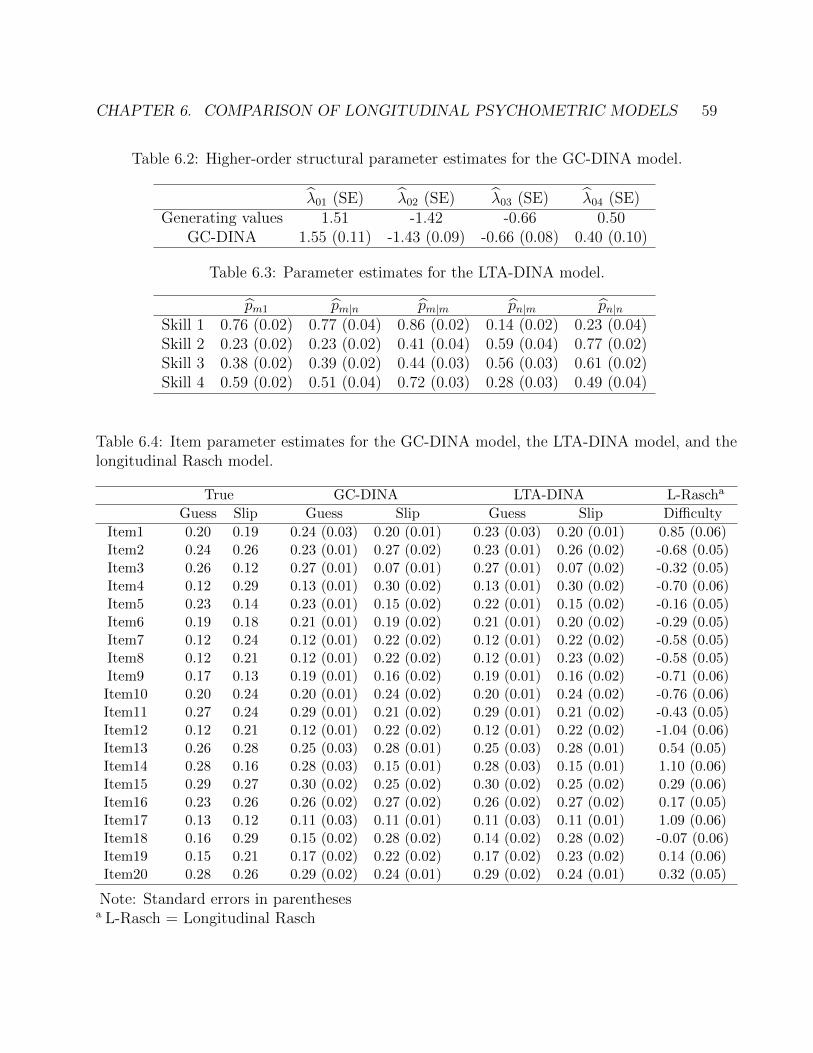
CHAPTER 6. COMPARISON OF LONGITUDINAL PSYCHOMETRIC MODELS 59
Table 6.2: Higher-order structural parameter estimates for the GC-DINA model.
λ01 (SE) λ02 (SE) λ03 (SE) λ04 (SE)Generating values 1.51 -1.42 -0.66 0.50
GC-DINA 1.55 (0.11) -1.43 (0.09) -0.66 (0.08) 0.40 (0.10)
Table 6.3: Parameter estimates for the LTA-DINA model.
pm1 pm|n pm|m pn|m pn|nSkill 1 0.76 (0.02) 0.77 (0.04) 0.86 (0.02) 0.14 (0.02) 0.23 (0.04)Skill 2 0.23 (0.02) 0.23 (0.02) 0.41 (0.04) 0.59 (0.04) 0.77 (0.02)Skill 3 0.38 (0.02) 0.39 (0.02) 0.44 (0.03) 0.56 (0.03) 0.61 (0.02)Skill 4 0.59 (0.02) 0.51 (0.04) 0.72 (0.03) 0.28 (0.03) 0.49 (0.04)
Table 6.4: Item parameter estimates for the GC-DINA model, the LTA-DINA model, and thelongitudinal Rasch model.
True GC-DINA LTA-DINA L-Rascha
Guess Slip Guess Slip Guess Slip Difficulty
Item1 0.20 0.19 0.24 (0.03) 0.20 (0.01) 0.23 (0.03) 0.20 (0.01) 0.85 (0.06)Item2 0.24 0.26 0.23 (0.01) 0.27 (0.02) 0.23 (0.01) 0.26 (0.02) -0.68 (0.05)Item3 0.26 0.12 0.27 (0.01) 0.07 (0.01) 0.27 (0.01) 0.07 (0.02) -0.32 (0.05)Item4 0.12 0.29 0.13 (0.01) 0.30 (0.02) 0.13 (0.01) 0.30 (0.02) -0.70 (0.06)Item5 0.23 0.14 0.23 (0.01) 0.15 (0.02) 0.22 (0.01) 0.15 (0.02) -0.16 (0.05)Item6 0.19 0.18 0.21 (0.01) 0.19 (0.02) 0.21 (0.01) 0.20 (0.02) -0.29 (0.05)Item7 0.12 0.24 0.12 (0.01) 0.22 (0.02) 0.12 (0.01) 0.22 (0.02) -0.58 (0.05)Item8 0.12 0.21 0.12 (0.01) 0.22 (0.02) 0.12 (0.01) 0.23 (0.02) -0.58 (0.05)Item9 0.17 0.13 0.19 (0.01) 0.16 (0.02) 0.19 (0.01) 0.16 (0.02) -0.71 (0.06)Item10 0.20 0.24 0.20 (0.01) 0.24 (0.02) 0.20 (0.01) 0.24 (0.02) -0.76 (0.06)Item11 0.27 0.24 0.29 (0.01) 0.21 (0.02) 0.29 (0.01) 0.21 (0.02) -0.43 (0.05)Item12 0.12 0.21 0.12 (0.01) 0.22 (0.02) 0.12 (0.01) 0.22 (0.02) -1.04 (0.06)Item13 0.26 0.28 0.25 (0.03) 0.28 (0.01) 0.25 (0.03) 0.28 (0.01) 0.54 (0.05)Item14 0.28 0.16 0.28 (0.03) 0.15 (0.01) 0.28 (0.03) 0.15 (0.01) 1.10 (0.06)Item15 0.29 0.27 0.30 (0.02) 0.25 (0.02) 0.30 (0.02) 0.25 (0.02) 0.29 (0.06)Item16 0.23 0.26 0.26 (0.02) 0.27 (0.02) 0.26 (0.02) 0.27 (0.02) 0.17 (0.05)Item17 0.13 0.12 0.11 (0.03) 0.11 (0.01) 0.11 (0.03) 0.11 (0.01) 1.09 (0.06)Item18 0.16 0.29 0.15 (0.02) 0.28 (0.02) 0.14 (0.02) 0.28 (0.02) -0.07 (0.06)Item19 0.15 0.21 0.17 (0.02) 0.22 (0.02) 0.17 (0.02) 0.23 (0.02) 0.14 (0.06)Item20 0.28 0.26 0.29 (0.02) 0.24 (0.01) 0.29 (0.02) 0.24 (0.01) 0.32 (0.05)
Note: Standard errors in parenthesesa L-Rasch = Longitudinal Rasch
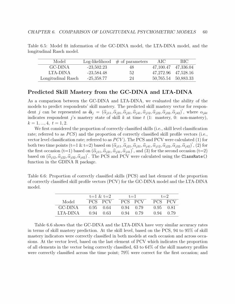
CHAPTER 6. COMPARISON OF LONGITUDINAL PSYCHOMETRIC MODELS 60
Table 6.5: Model fit information of the GC-DINA model, the LTA-DINA model, and thelongitudinal Rasch model.
Model Log-likelihood # of parameters AIC BICGC-DINA -23,502.23 48 47,100.47 47,336.04LTA-DINA -23,584.48 52 47,272.96 47,528.16
Longitudinal Rasch -25,358.77 24 50,765.54 50,883.33
Predicted Skill Mastery from the GC-DINA and LTA-DINA
As a comparison between the GC-DINA and LTA-DINA, we evaluated the ability of themodels to predict respondents’ skill mastery. The predicted skill mastery vector for respon-dent j can be represented as αj = (αj11, αj21, αj31, αj41, αj12, αj22, αj32, αj42)
′, where αjkt
indicates respondent j’s mastery state of skill k at time t (1: mastery, 0: non-mastery),k = 1, ..., 4, t = 1, 2.
We first considered the proportion of correctly classified skills (i.e., skill level classificationrate; referred to as PCS ) and the proportion of correctly classified skill profile vectors (i.e.,vector level classification rate; referred to as PCV ). The PCS and PCV were calculated (1) forboth two time points (t=1 & t=2) based on (αj11, αj21, αj31, αj41, αj12, αj22, αj32, αj42)
′, (2) for
the first occasion (t=1) based on (αj11, αj21, αj31, αj41)′, and (3) for the second occasion (t=2)
based on (αj12, αj22, αj32, αj42)′. The PCS and PCV were calculated using the ClassRate()
function in the GDINA R package.
Table 6.6: Proportion of correctly classified skills (PCS) and last element of the proportionof correctly classified skill profile vectors (PCV) for the GC-DINA model and the LTA-DINAmodel.
t=1 & t=2 t=1 t=2Model PCS PCV PCS PCV PCS PCV
GC-DINA 0.95 0.64 0.94 0.79 0.95 0.81LTA-DINA 0.94 0.63 0.94 0.79 0.94 0.79
Table 6.6 shows that the GC-DINA and the LTA-DINA have very similar accuracy ratesin terms of skill mastery prediction. At the skill level, based on the PCS, 94 to 95% of skillmastery indicators were correctly classified in both models at each occasion and across occa-sions. At the vector level, based on the last element of PCV which indicates the proportionof all elements in the vector being correctly classified, 63 to 64% of the skill mastery profileswere correctly classified across the time point; 79% were correct for the first occasion; and
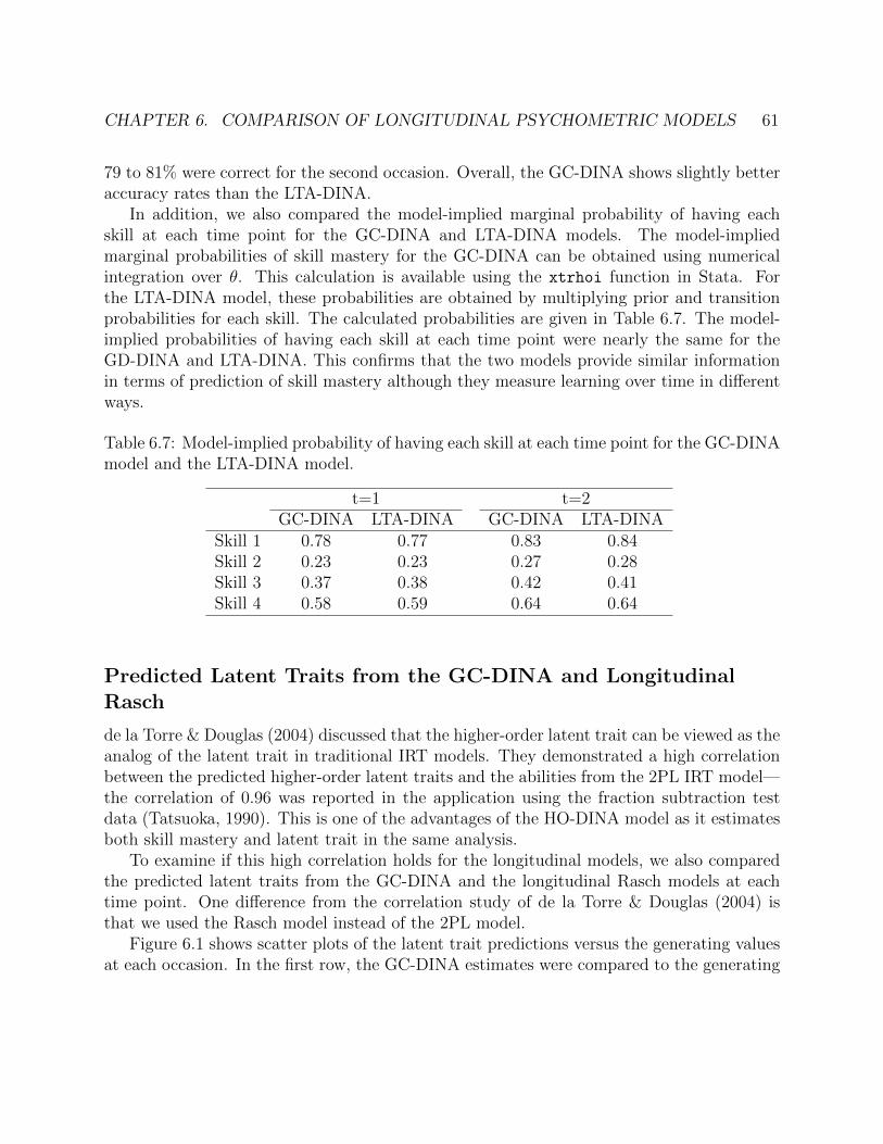
CHAPTER 6. COMPARISON OF LONGITUDINAL PSYCHOMETRIC MODELS 61
79 to 81% were correct for the second occasion. Overall, the GC-DINA shows slightly betteraccuracy rates than the LTA-DINA.
In addition, we also compared the model-implied marginal probability of having eachskill at each time point for the GC-DINA and LTA-DINA models. The model-impliedmarginal probabilities of skill mastery for the GC-DINA can be obtained using numericalintegration over θ. This calculation is available using the xtrhoi function in Stata. Forthe LTA-DINA model, these probabilities are obtained by multiplying prior and transitionprobabilities for each skill. The calculated probabilities are given in Table 6.7. The model-implied probabilities of having each skill at each time point were nearly the same for theGD-DINA and LTA-DINA. This confirms that the two models provide similar informationin terms of prediction of skill mastery although they measure learning over time in differentways.
Table 6.7: Model-implied probability of having each skill at each time point for the GC-DINAmodel and the LTA-DINA model.
t=1 t=2GC-DINA LTA-DINA GC-DINA LTA-DINA
Skill 1 0.78 0.77 0.83 0.84Skill 2 0.23 0.23 0.27 0.28Skill 3 0.37 0.38 0.42 0.41Skill 4 0.58 0.59 0.64 0.64
Predicted Latent Traits from the GC-DINA and LongitudinalRasch
de la Torre & Douglas (2004) discussed that the higher-order latent trait can be viewed as theanalog of the latent trait in traditional IRT models. They demonstrated a high correlationbetween the predicted higher-order latent traits and the abilities from the 2PL IRT model—the correlation of 0.96 was reported in the application using the fraction subtraction testdata (Tatsuoka, 1990). This is one of the advantages of the HO-DINA model as it estimatesboth skill mastery and latent trait in the same analysis.
To examine if this high correlation holds for the longitudinal models, we also comparedthe predicted latent traits from the GC-DINA and the longitudinal Rasch models at eachtime point. One difference from the correlation study of de la Torre & Douglas (2004) isthat we used the Rasch model instead of the 2PL model.
Figure 6.1 shows scatter plots of the latent trait predictions versus the generating valuesat each occasion. In the first row, the GC-DINA estimates were compared to the generating
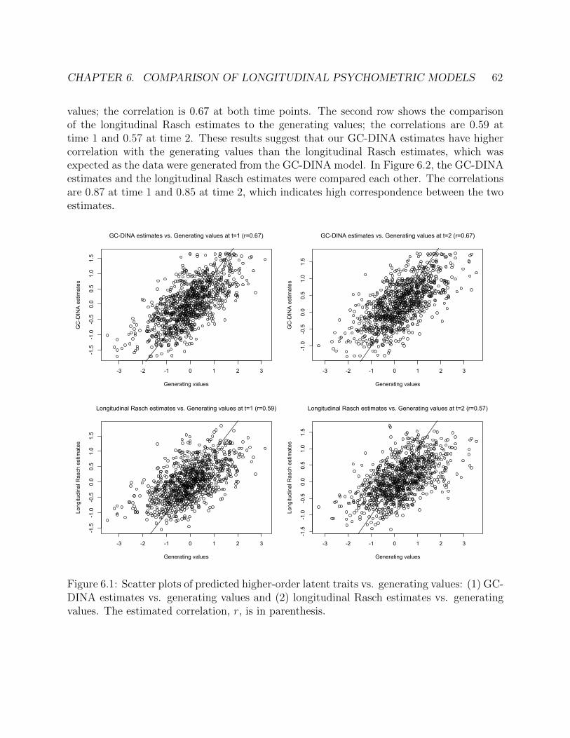
CHAPTER 6. COMPARISON OF LONGITUDINAL PSYCHOMETRIC MODELS 62
values; the correlation is 0.67 at both time points. The second row shows the comparisonof the longitudinal Rasch estimates to the generating values; the correlations are 0.59 attime 1 and 0.57 at time 2. These results suggest that our GC-DINA estimates have highercorrelation with the generating values than the longitudinal Rasch estimates, which wasexpected as the data were generated from the GC-DINA model. In Figure 6.2, the GC-DINAestimates and the longitudinal Rasch estimates were compared each other. The correlationsare 0.87 at time 1 and 0.85 at time 2, which indicates high correspondence between the twoestimates.
-3 -2 -1 0 1 2 3
-1.5
-1.0
-0.5
0.0
0.5
1.0
1.5
Generating values
GC
-DIN
A e
stim
ates
GC-DINA estimates vs. Generating values at t=1 (r=0.67)
-3 -2 -1 0 1 2 3
-1.0
-0.5
0.0
0.5
1.0
1.5
Generating values
GC
-DIN
A e
stim
ates
GC-DINA estimates vs. Generating values at t=2 (r=0.67)
-3 -2 -1 0 1 2 3
-1.5
-1.0
-0.5
0.0
0.5
1.0
1.5
Generating values
Long
itudi
nal R
asch
est
imat
es
Longitudinal Rasch estimates vs. Generating values at t=1 (r=0.59)
-3 -2 -1 0 1 2 3
-1.5
-1.0
-0.5
0.0
0.5
1.0
1.5
Generating values
Long
itudi
nal R
asch
est
imat
es
Longitudinal Rasch estimates vs. Generating values at t=2 (r=0.57)
Figure 6.1: Scatter plots of predicted higher-order latent traits vs. generating values: (1) GC-DINA estimates vs. generating values and (2) longitudinal Rasch estimates vs. generatingvalues. The estimated correlation, r, is in parenthesis.
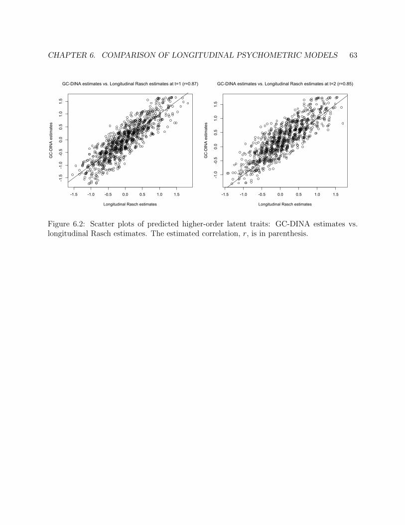
CHAPTER 6. COMPARISON OF LONGITUDINAL PSYCHOMETRIC MODELS 63
-1.5 -1.0 -0.5 0.0 0.5 1.0 1.5
-1.5
-1.0
-0.5
0.0
0.5
1.0
1.5
Longitudinal Rasch estimates
GC
-DIN
A e
stim
ates
GC-DINA estimates vs. Longitudinal Rasch estimates at t=1 (r=0.87)
-1.5 -1.0 -0.5 0.0 0.5 1.0 1.5
-1.0
-0.5
0.0
0.5
1.0
1.5
Longitudinal Rasch estimatesG
C-D
INA
est
imat
es
GC-DINA estimates vs. Longitudinal Rasch estimates at t=2 (r=0.85)
Figure 6.2: Scatter plots of predicted higher-order latent traits: GC-DINA estimates vs.longitudinal Rasch estimates. The estimated correlation, r, is in parenthesis.
64
Chapter 7
Conclusion
In this dissertation, GC-CDMs were proposed to incorporate learning over time into thecognitive assessment framework. GC-CDMs include a higher-order latent trait interpretableas a more broadly defined general ability associated with skills, and the relationship betweenthe higher-order latent trait and skills can be specified by the Rasch model, i.e., skills playthe role of items and skill masteries for different skills are conditionally independent giventhe higher-order latent trait. GC-CDMs trace changes in the higher-order latent trait overtime by latent growth modeling, and simultaneously trace students’ skill mastery throughthe CDM measurement model.
For estimation of GC-CDMs, we used marginal likelihood estimation with the nestedintegration to lessen the high-dimensional computation problem. By using the nested inte-gration, the likelihood has the same structure as a multilevel model in which occasions arenested within persons, and the MLE requires only 3-dimensional integration regardless ofthe number of time points.
Relevant issues for estimating GC-CDMs were also discussed. In terms of modeling therelationship between the higher-order latent trait and the multiple skills, we showed that,for the case of a single time point, parameters of the HO-DINA model were estimated moreprecisely when using the Rasch model than when using the 2PL model. In addition, weaddressed the model identification issue when only two time points are available. In suchcases, we suggested an alternative approach of using a bivariate normal distribution to modelthe correlation between the higher-order latent traits at the two occasions.
Through simulation studies, parameter recovery of the GC-DINA model was examined.In the first simulation study, we focused on parameter recovery under differing conditionsto investigate the effects of the following factors on model estimates: the design of the Q-matrix, the number of respondents and the number of time points. We found that the pointestimates deteriorated when switching from the simple to the complex Q-matrix; and thestandard errors of the estimates increased for the smaller sample size. We did not observe a
CHAPTER 7. CONCLUSION 65
significant effect of the number of time points based on the comparison between three timepoints and four time points. Overall, across all conditions, the GC-DINA model estimatesshowed good recovery, especially the average growth (which is the parameter of interest).The results imply that the simpler design of the Q-matrix and larger sample size would bepreferable for better estimates of GC-CDMs. However, this conclusion is tentative becausethese results were based on only on replication per model. In the second simulation study, wefocused on the analysis of pre-post assessment data when only two time points are available.The GC-DINA defined for two time points was applied, and it had good parameter recovery.
The application of the GC-DINA model to real data was illustrated by using two datasetsfrom multi-wave experiments designed to assess the effects of EAI treatments on mathematicsachievement. Both the regular GC-DINA model and the GC-DINA model for two time pointswere applied and provided useful interpretations in terms of both growth in the higher-orderlatent trait and changes in skill mastery status over time.
Another contribution of this dissertation is a review of the literature on other longitudinalpsychometric models—longitudinal IRT models, latent transition analysis with CDMs anddynamic Bayesian Networks. Then we examined similarities among the GC-CDM, the LTA-CDM and the longitudinal IRT model in a simulation study. Using a simulated data for twooccasions from the GC-DINA model, we compared the GC-DINA model, the LTA-DINAmodel and the longitudinal IRT model. We found similarities between the GC-DINA modeland the LTA-DINA model in terms of the predicted skill mastery; and between the GC-DINA model and the longitudinal IRT model in terms of the predicted higher-order latenttrait.
There are several potential avenues for future work. In terms of model performance,future research could investigate how to improve the efficiency of estimation and developmodel diagnostics for GC-CDMs. In addition, the possible extensions discussed in Section 3could be further investigated. Specifically, it would be interesting to (1) allow skill and timespecific learning and (2) incorporatie respondents’ covariates into the model.
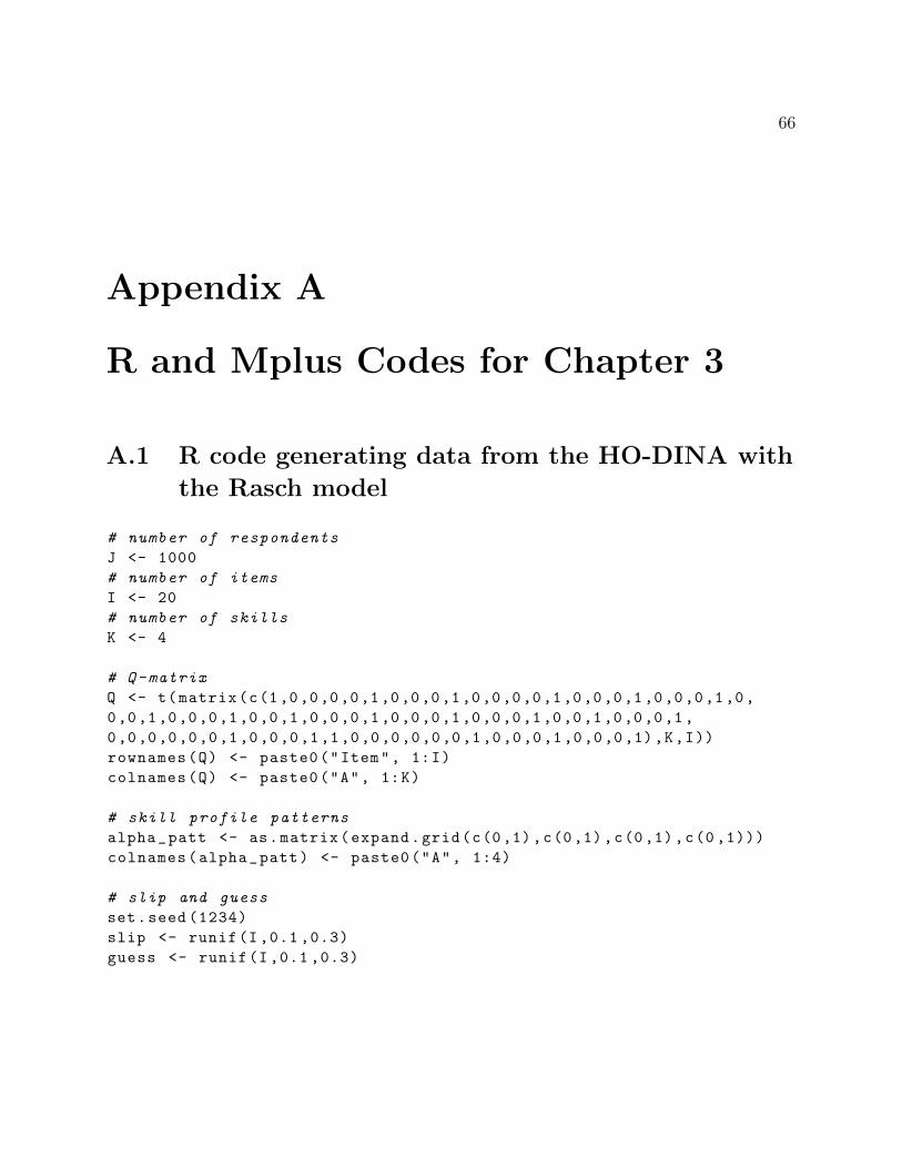
66
Appendix A
R and Mplus Codes for Chapter 3
A.1 R code generating data from the HO-DINA with
the Rasch model
# number of respondents
J <- 1000
# number of items
I <- 20
# number of skills
K <- 4
# Q-matrix
Q <- t(matrix(c(1,0,0,0,0,1,0,0,0,1,0,0,0,0,1,0,0,0,1,0,0,0,1,0,
0,0,1,0,0,0,1,0,0,1,0,0,0,1,0,0,0,1,0,0,0,1,0,0,1,0,0,0,1,
0,0,0,0,0,0,1,0,0,0,1,1,0,0,0,0,0,0,1,0,0,0,1,0,0,0,1),K,I))
rownames(Q) <- paste0("Item", 1:I)
colnames(Q) <- paste0("A", 1:K)
# skill profile patterns
alpha_patt <- as.matrix(expand.grid(c(0,1),c(0,1),c(0,1),c(0 ,1)))
colnames(alpha_patt) <- paste0("A", 1:4)
# slip and guess
set.seed (1234)
slip <- runif(I,0.1 ,0.3)
guess <- runif(I,0.1 ,0.3)
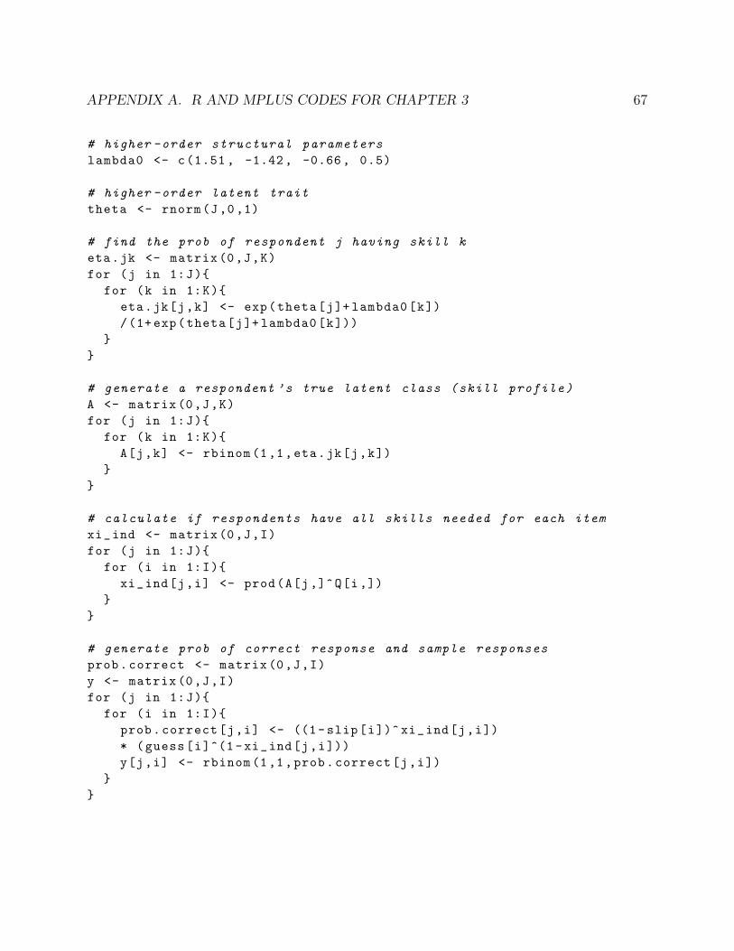
APPENDIX A. R AND MPLUS CODES FOR CHAPTER 3 67
# higher -order structural parameters
lambda0 <- c(1.51, -1.42, -0.66, 0.5)
# higher -order latent trait
theta <- rnorm(J,0,1)
# find the prob of respondent j having skill k
eta.jk <- matrix(0,J,K)
for (j in 1:J){
for (k in 1:K){
eta.jk[j,k] <- exp(theta[j]+ lambda0[k])
/(1+exp(theta[j]+ lambda0[k]))
}
}
# generate a respondent ’s true latent class (skill profile)
A <- matrix(0,J,K)
for (j in 1:J){
for (k in 1:K){
A[j,k] <- rbinom(1,1,eta.jk[j,k])
}
}
# calculate if respondents have all skills needed for each item
xi_ind <- matrix(0,J,I)
for (j in 1:J){
for (i in 1:I){
xi_ind[j,i] <- prod(A[j,]^Q[i,])
}
}
# generate prob of correct response and sample responses
prob.correct <- matrix(0,J,I)
y <- matrix(0,J,I)
for (j in 1:J){
for (i in 1:I){
prob.correct[j,i] <- ((1-slip[i])^xi_ind[j,i])
* (guess[i]^(1-xi_ind[j,i]))
y[j,i] <- rbinom(1,1,prob.correct[j,i])
}
}
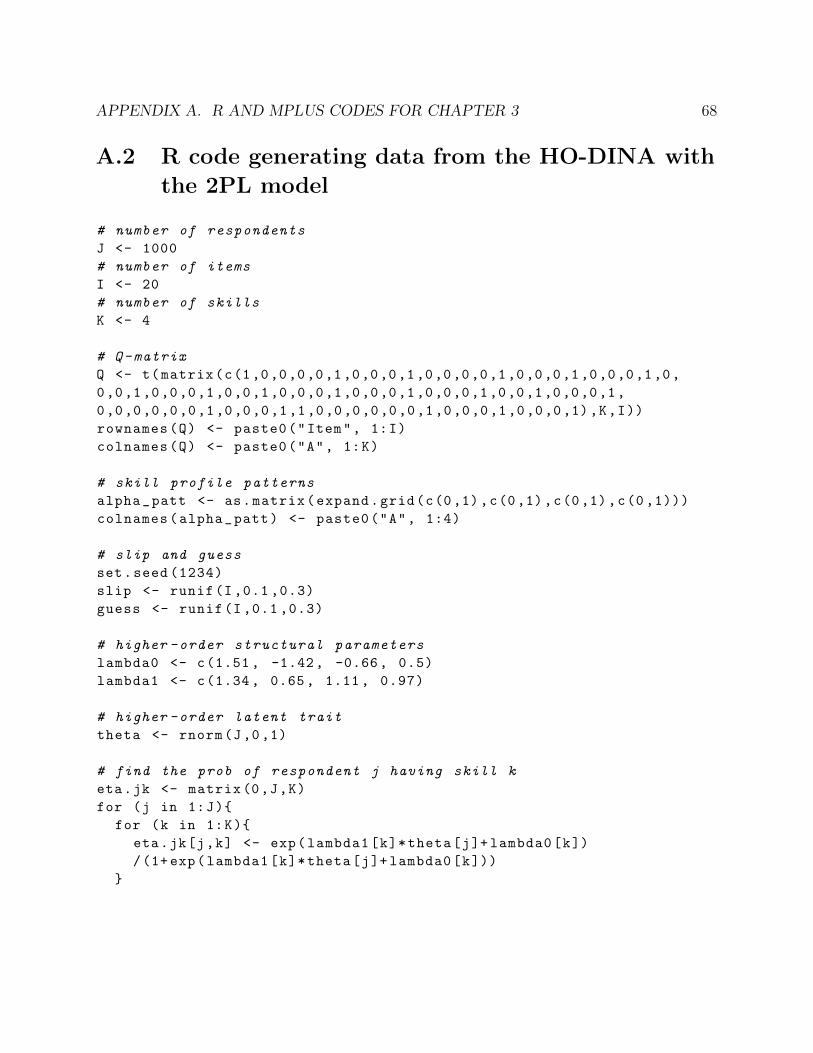
APPENDIX A. R AND MPLUS CODES FOR CHAPTER 3 68
A.2 R code generating data from the HO-DINA with
the 2PL model
# number of respondents
J <- 1000
# number of items
I <- 20
# number of skills
K <- 4
# Q-matrix
Q <- t(matrix(c(1,0,0,0,0,1,0,0,0,1,0,0,0,0,1,0,0,0,1,0,0,0,1,0,
0,0,1,0,0,0,1,0,0,1,0,0,0,1,0,0,0,1,0,0,0,1,0,0,1,0,0,0,1,
0,0,0,0,0,0,1,0,0,0,1,1,0,0,0,0,0,0,1,0,0,0,1,0,0,0,1),K,I))
rownames(Q) <- paste0("Item", 1:I)
colnames(Q) <- paste0("A", 1:K)
# skill profile patterns
alpha_patt <- as.matrix(expand.grid(c(0,1),c(0,1),c(0,1),c(0 ,1)))
colnames(alpha_patt) <- paste0("A", 1:4)
# slip and guess
set.seed (1234)
slip <- runif(I,0.1 ,0.3)
guess <- runif(I,0.1 ,0.3)
# higher -order structural parameters
lambda0 <- c(1.51, -1.42, -0.66, 0.5)
lambda1 <- c(1.34, 0.65, 1.11, 0.97)
# higher -order latent trait
theta <- rnorm(J,0,1)
# find the prob of respondent j having skill k
eta.jk <- matrix(0,J,K)
for (j in 1:J){
for (k in 1:K){
eta.jk[j,k] <- exp(lambda1[k]*theta[j]+ lambda0[k])
/(1+exp(lambda1[k]*theta[j]+ lambda0[k]))
}
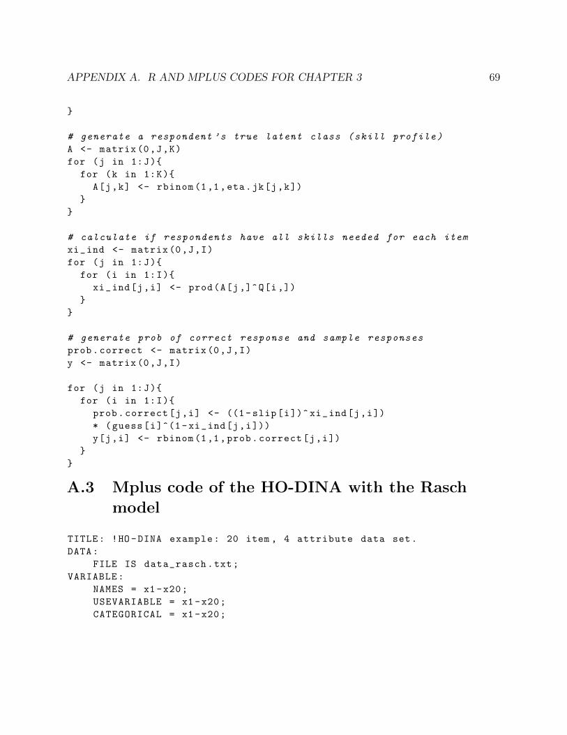
APPENDIX A. R AND MPLUS CODES FOR CHAPTER 3 69
}
# generate a respondent ’s true latent class (skill profile)
A <- matrix(0,J,K)
for (j in 1:J){
for (k in 1:K){
A[j,k] <- rbinom(1,1,eta.jk[j,k])
}
}
# calculate if respondents have all skills needed for each item
xi_ind <- matrix(0,J,I)
for (j in 1:J){
for (i in 1:I){
xi_ind[j,i] <- prod(A[j,]^Q[i,])
}
}
# generate prob of correct response and sample responses
prob.correct <- matrix(0,J,I)
y <- matrix(0,J,I)
for (j in 1:J){
for (i in 1:I){
prob.correct[j,i] <- ((1-slip[i])^xi_ind[j,i])
* (guess[i]^(1-xi_ind[j,i]))
y[j,i] <- rbinom(1,1,prob.correct[j,i])
}
}
A.3 Mplus code of the HO-DINA with the Rasch
model
TITLE: !HO -DINA example: 20 item , 4 attribute data set.
DATA:
FILE IS data_rasch.txt;
VARIABLE:
NAMES = x1-x20;
USEVARIABLE = x1-x20;
CATEGORICAL = x1-x20;
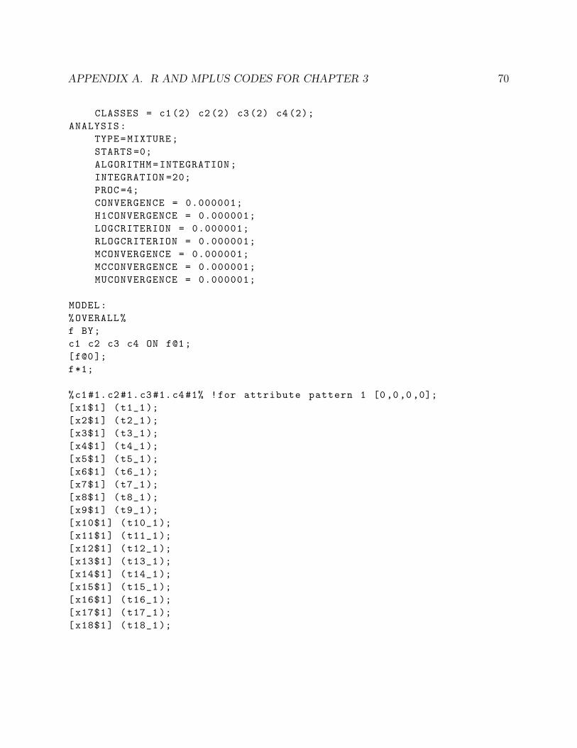
APPENDIX A. R AND MPLUS CODES FOR CHAPTER 3 70
CLASSES = c1(2) c2(2) c3(2) c4(2);
ANALYSIS:
TYPE=MIXTURE;
STARTS =0;
ALGORITHM=INTEGRATION;
INTEGRATION =20;
PROC =4;
CONVERGENCE = 0.000001;
H1CONVERGENCE = 0.000001;
LOGCRITERION = 0.000001;
RLOGCRITERION = 0.000001;
MCONVERGENCE = 0.000001;
MCCONVERGENCE = 0.000001;
MUCONVERGENCE = 0.000001;
MODEL:
%OVERALL%
f BY;
c1 c2 c3 c4 ON f@1;
[f@0];
f*1;
%c1#1.c2#1.c3#1.c4#1% !for attribute pattern 1 [0,0,0,0];
[x1$1] (t1_1);
[x2$1] (t2_1);
[x3$1] (t3_1);
[x4$1] (t4_1);
[x5$1] (t5_1);
[x6$1] (t6_1);
[x7$1] (t7_1);
[x8$1] (t8_1);
[x9$1] (t9_1);
[x10$1] (t10_1 );
[x11$1] (t11_1 );
[x12$1] (t12_1 );
[x13$1] (t13_1 );
[x14$1] (t14_1 );
[x15$1] (t15_1 );
[x16$1] (t16_1 );
[x17$1] (t17_1 );
[x18$1] (t18_1 );
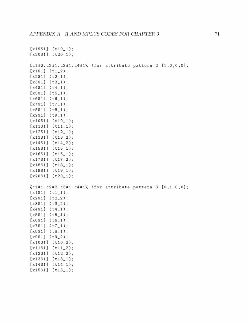
APPENDIX A. R AND MPLUS CODES FOR CHAPTER 3 71
[x19$1] (t19_1 );
[x20$1] (t20_1 );
%c1#2.c2#1.c3#1.c4#1% !for attribute pattern 2 [1,0,0,0];
[x1$1] (t1_2);
[x2$1] (t2_1);
[x3$1] (t3_1);
[x4$1] (t4_1);
[x5$1] (t5_1);
[x6$1] (t6_1);
[x7$1] (t7_1);
[x8$1] (t8_1);
[x9$1] (t9_1);
[x10$1] (t10_1 );
[x11$1] (t11_1 );
[x12$1] (t12_1 );
[x13$1] (t13_2 );
[x14$1] (t14_2 );
[x15$1] (t15_1 );
[x16$1] (t16_1 );
[x17$1] (t17_2 );
[x18$1] (t18_1 );
[x19$1] (t19_1 );
[x20$1] (t20_1 );
%c1#1.c2#2.c3#1.c4#1% !for attribute pattern 3 [0,1,0,0];
[x1$1] (t1_1);
[x2$1] (t2_2);
[x3$1] (t3_2);
[x4$1] (t4_1);
[x5$1] (t5_1);
[x6$1] (t6_1);
[x7$1] (t7_1);
[x8$1] (t8_1);
[x9$1] (t9_2);
[x10$1] (t10_2 );
[x11$1] (t11_2 );
[x12$1] (t12_2 );
[x13$1] (t13_1 );
[x14$1] (t14_1 );
[x15$1] (t15_1 );

APPENDIX A. R AND MPLUS CODES FOR CHAPTER 3 72
[x16$1] (t16_1 );
[x17$1] (t17_1 );
[x18$1] (t18_1 );
[x19$1] (t19_1 );
[x20$1] (t20_1 );
%c1#1.c2#1.c3#2.c4#1% !for attribute pattern 4 [0,0,1,0];
[x1$1] (t1_1);
[x2$1] (t2_1);
[x3$1] (t3_1);
[x4$1] (t4_2);
[x5$1] (t5_2);
[x6$1] (t6_2);
[x7$1] (t7_2);
[x8$1] (t8_2);
[x9$1] (t9_1);
[x10$1] (t10_1 );
[x11$1] (t11_1 );
[x12$1] (t12_1 );
[x13$1] (t13_1 );
[x14$1] (t14_1 );
[x15$1] (t15_1 );
[x16$1] (t16_1 );
[x17$1] (t17_1 );
[x18$1] (t18_1 );
[x19$1] (t19_1 );
[x20$1] (t20_1 );
%c1#1.c2#1.c3#1.c4#2% !for attribute pattern 5 [0,0,0,1];
[x1$1] (t1_1);
[x2$1] (t2_1);
[x3$1] (t3_1);
[x4$1] (t4_1);
[x5$1] (t5_1);
[x6$1] (t6_1);
[x7$1] (t7_1);
[x8$1] (t8_1);
[x9$1] (t9_1);
[x10$1] (t10_1 );
[x11$1] (t11_1 );
[x12$1] (t12_1 );

APPENDIX A. R AND MPLUS CODES FOR CHAPTER 3 73
[x13$1] (t13_1 );
[x14$1] (t14_1 );
[x15$1] (t15_2 );
[x16$1] (t16_2 );
[x17$1] (t17_1 );
[x18$1] (t18_2 );
[x19$1] (t19_2 );
[x20$1] (t20_2 );
%c1#2.c2#2.c3#1.c4#1% !for attribute pattern 6 [1,1,0,0];
[x1$1] (t1_2);
[x2$1] (t2_2);
[x3$1] (t3_2);
[x4$1] (t4_1);
[x5$1] (t5_1);
[x6$1] (t6_1);
[x7$1] (t7_1);
[x8$1] (t8_1);
[x9$1] (t9_2);
[x10$1] (t10_2 );
[x11$1] (t11_2 );
[x12$1] (t12_2 );
[x13$1] (t13_2 );
[x14$1] (t14_2 );
[x15$1] (t15_1 );
[x16$1] (t16_1 );
[x17$1] (t17_2 );
[x18$1] (t18_1 );
[x19$1] (t19_1 );
[x20$1] (t20_1 );
%c1#2.c2#1.c3#2.c4#1% !for attribute pattern 7 [1,0,1,0];
[x1$1] (t1_2);
[x2$1] (t2_1);
[x3$1] (t3_1);
[x4$1] (t4_2);
[x5$1] (t5_2);
[x6$1] (t6_2);
[x7$1] (t7_2);
[x8$1] (t8_2);
[x9$1] (t9_1);

APPENDIX A. R AND MPLUS CODES FOR CHAPTER 3 74
[x10$1] (t10_1 );
[x11$1] (t11_1 );
[x12$1] (t12_1 );
[x13$1] (t13_2 );
[x14$1] (t14_2 );
[x15$1] (t15_1 );
[x16$1] (t16_1 );
[x17$1] (t17_2 );
[x18$1] (t18_1 );
[x19$1] (t19_1 );
[x20$1] (t20_1 );
%c1#2.c2#1.c3#1.c4#2% !for attribute pattern 8 [1,0,0,1];
[x1$1] (t1_2);
[x2$1] (t2_1);
[x3$1] (t3_1);
[x4$1] (t4_1);
[x5$1] (t5_1);
[x6$1] (t6_1);
[x7$1] (t7_1);
[x8$1] (t8_1);
[x9$1] (t9_1);
[x10$1] (t10_1 );
[x11$1] (t11_1 );
[x12$1] (t12_1 );
[x13$1] (t13_2 );
[x14$1] (t14_2 );
[x15$1] (t15_2 );
[x16$1] (t16_2 );
[x17$1] (t17_2 );
[x18$1] (t18_2 );
[x19$1] (t19_2 );
[x20$1] (t20_2 );
%c1#1.c2#2.c3#2.c4#1% !for attribute pattern 9 [0,1,1,0];
[x1$1] (t1_1);
[x2$1] (t2_2);
[x3$1] (t3_2);
[x4$1] (t4_2);
[x5$1] (t5_2);
[x6$1] (t6_2);

APPENDIX A. R AND MPLUS CODES FOR CHAPTER 3 75
[x7$1] (t7_2);
[x8$1] (t8_2);
[x9$1] (t9_2);
[x10$1] (t10_2 );
[x11$1] (t11_2 );
[x12$1] (t12_2 );
[x13$1] (t13_1 );
[x14$1] (t14_1 );
[x15$1] (t15_1 );
[x16$1] (t16_1 );
[x17$1] (t17_1 );
[x18$1] (t18_1 );
[x19$1] (t19_1 );
[x20$1] (t20_1 );
%c1#1.c2#2.c3#1.c4#2% !for attribute pattern 10 [0,1,0,1];
[x1$1] (t1_1);
[x2$1] (t2_2);
[x3$1] (t3_2);
[x4$1] (t4_1);
[x5$1] (t5_1);
[x6$1] (t6_1);
[x7$1] (t7_1);
[x8$1] (t8_1);
[x9$1] (t9_2);
[x10$1] (t10_2 );
[x11$1] (t11_2 );
[x12$1] (t12_2 );
[x13$1] (t13_1 );
[x14$1] (t14_1 );
[x15$1] (t15_2 );
[x16$1] (t16_2 );
[x17$1] (t17_1 );
[x18$1] (t18_2 );
[x19$1] (t19_2 );
[x20$1] (t20_2 );
%c1#1.c2#1.c3#2.c4#2% !for attribute pattern 11 [0,0,1,1];
[x1$1] (t1_1);
[x2$1] (t2_1);
[x3$1] (t3_1);

APPENDIX A. R AND MPLUS CODES FOR CHAPTER 3 76
[x4$1] (t4_2);
[x5$1] (t5_2);
[x6$1] (t6_2);
[x7$1] (t7_2);
[x8$1] (t8_2);
[x9$1] (t9_1);
[x10$1] (t10_1 );
[x11$1] (t11_1 );
[x12$1] (t12_1 );
[x13$1] (t13_1 );
[x14$1] (t14_1 );
[x15$1] (t15_2 );
[x16$1] (t16_2 );
[x17$1] (t17_1 );
[x18$1] (t18_2 );
[x19$1] (t19_2 );
[x20$1] (t20_2 );
%c1#2.c2#2.c3#2.c4#1% !for attribute pattern 12 [1,1,1,0];
[x1$1] (t1_2);
[x2$1] (t2_2);
[x3$1] (t3_2);
[x4$1] (t4_2);
[x5$1] (t5_2);
[x6$1] (t6_2);
[x7$1] (t7_2);
[x8$1] (t8_2);
[x9$1] (t9_2);
[x10$1] (t10_2 );
[x11$1] (t11_2 );
[x12$1] (t12_2 );
[x13$1] (t13_2 );
[x14$1] (t14_2 );
[x15$1] (t15_1 );
[x16$1] (t16_1 );
[x17$1] (t17_2 );
[x18$1] (t18_1 );
[x19$1] (t19_1 );
[x20$1] (t20_1 );
%c1#2.c2#2.c3#1.c4#2% !for attribute pattern 13 [1,1,0,1];
APPENDIX A. R AND MPLUS CODES FOR CHAPTER 3 77
[x1$1] (t1_2);
[x2$1] (t2_2);
[x3$1] (t3_2);
[x4$1] (t4_1);
[x5$1] (t5_1);
[x6$1] (t6_1);
[x7$1] (t7_1);
[x8$1] (t8_1);
[x9$1] (t9_2);
[x10$1] (t10_2 );
[x11$1] (t11_2 );
[x12$1] (t12_2 );
[x13$1] (t13_2 );
[x14$1] (t14_2 );
[x15$1] (t15_2 );
[x16$1] (t16_2 );
[x17$1] (t17_2 );
[x18$1] (t18_2 );
[x19$1] (t19_2 );
[x20$1] (t20_2 );
%c1#2.c2#1.c3#2.c4#2% !for attribute pattern 14 [1,0,1,1];
[x1$1] (t1_2);
[x2$1] (t2_1);
[x3$1] (t3_1);
[x4$1] (t4_2);
[x5$1] (t5_2);
[x6$1] (t6_2);
[x7$1] (t7_2);
[x8$1] (t8_2);
[x9$1] (t9_1);
[x10$1] (t10_1 );
[x11$1] (t11_1 );
[x12$1] (t12_1 );
[x13$1] (t13_2 );
[x14$1] (t14_2 );
[x15$1] (t15_2 );
[x16$1] (t16_2 );
[x17$1] (t17_2 );
[x18$1] (t18_2 );
[x19$1] (t19_2 );
APPENDIX A. R AND MPLUS CODES FOR CHAPTER 3 78
[x20$1] (t20_2 );
%c1#1.c2#2.c3#2.c4#2% !for attribute pattern 15 [0,1,1,1];
[x1$1] (t1_1);
[x2$1] (t2_2);
[x3$1] (t3_2);
[x4$1] (t4_2);
[x5$1] (t5_2);
[x6$1] (t6_2);
[x7$1] (t7_2);
[x8$1] (t8_2);
[x9$1] (t9_2);
[x10$1] (t10_2 );
[x11$1] (t11_2 );
[x12$1] (t12_2 );
[x13$1] (t13_1 );
[x14$1] (t14_1 );
[x15$1] (t15_2 );
[x16$1] (t16_2 );
[x17$1] (t17_1 );
[x18$1] (t18_2 );
[x19$1] (t19_2 );
[x20$1] (t20_2 );
%c1#2.c2#2.c3#2.c4#2% !for attribute pattern 16 [1,1,1,1];
[x1$1] (t1_2);
[x2$1] (t2_2);
[x3$1] (t3_2);
[x4$1] (t4_2);
[x5$1] (t5_2);
[x6$1] (t6_2);
[x7$1] (t7_2);
[x8$1] (t8_2);
[x9$1] (t9_2);
[x10$1] (t10_2 );
[x11$1] (t11_2 );
[x12$1] (t12_2 );
[x13$1] (t13_2 );
[x14$1] (t14_2 );
[x15$1] (t15_2 );
[x16$1] (t16_2 );
APPENDIX A. R AND MPLUS CODES FOR CHAPTER 3 79
[x17$1] (t17_2 );
[x18$1] (t18_2 );
[x19$1] (t19_2 );
[x20$1] (t20_2 );
MODEL CONSTRAINT:
!ITEM 1:
NEW(l1_0 l1_e);
t1_1=-(l1_0);
t1_2=-(l1_0+l1_e);
l1_e >0;
!ITEM 2:
NEW(l2_0 l2_e);
t2_1=-(l2_0);
t2_2=-(l2_0+l2_e);
l2_e >0;
!ITEM 3:
NEW(l3_0 l3_e);
t3_1=-(l3_0);
t3_2=-(l3_0+l3_e);
l3_e >0;
!ITEM 4:
NEW(l4_0 l4_e);
t4_1=-(l4_0);
t4_2=-(l4_0+l4_e);
l4_e >0;
!ITEM 5:
NEW(l5_0 l5_e);
t5_1=-(l5_0);
t5_2=-(l5_0+l5_e);
l5_e >0;
!ITEM 6:
NEW(l6_0 l6_e);
t6_1=-(l6_0);
t6_2=-(l6_0+l6_e);

APPENDIX A. R AND MPLUS CODES FOR CHAPTER 3 80
l6_e >0;
!ITEM 7:
NEW(l7_0 l7_e);
t7_1=-(l7_0);
t7_2=-(l7_0+l7_e);
l7_e >0;
!ITEM 8:
NEW(l8_0 l8_e);
t8_1=-(l8_0);
t8_2=-(l8_0+l8_e);
l8_e >0;
!ITEM 9:
NEW(l9_0 l9_e);
t9_1=-(l9_0);
t9_2=-(l9_0+l9_e);
l9_e >0;
!ITEM 10:
NEW(l10_0 l10_e);
t10_1=-(l10_0);
t10_2=-(l10_0+l10_e);
l10_e >0;
!ITEM 11:
NEW(l11_0 l11_e);
t11_1=-(l11_0);
t11_2=-(l11_0+l11_e);
l11_e >0;
!ITEM 12:
NEW(l12_0 l12_e);
t12_1=-(l12_0);
t12_2=-(l12_0+l12_e);
l12_e >0;
!ITEM 13:
NEW(l13_0 l13_e);
t13_1=-(l13_0);
APPENDIX A. R AND MPLUS CODES FOR CHAPTER 3 81
t13_2=-(l13_0+l13_e);
l13_e >0;
!ITEM 14:
NEW(l14_0 l14_e);
t14_1=-(l14_0);
t14_2=-(l14_0+l14_e);
l14_e >0;
!ITEM 15:
NEW(l15_0 l15_e);
t15_1=-(l15_0);
t15_2=-(l15_0+l15_e);
l15_e >0;
!ITEM 16:
NEW(l16_0 l16_e);
t16_1=-(l16_0);
t16_2=-(l16_0+l16_e);
l16_e >0;
!ITEM 17:
NEW(l17_0 l17_e);
t17_1=-(l17_0);
t17_2=-(l17_0+l17_e);
l17_e >0;
!ITEM 18:
NEW(l18_0 l18_e);
t18_1=-(l18_0);
t18_2=-(l18_0+l18_e);
l18_e >0;
!ITEM 19:
NEW(l19_0 l19_e);
t19_1=-(l19_0);
t19_2=-(l19_0+l19_e);
l19_e >0;
!ITEM 20:
NEW(l20_0 l20_e);
APPENDIX A. R AND MPLUS CODES FOR CHAPTER 3 82
t20_1=-(l20_0);
t20_2=-(l20_0+l20_e);
l20_e >0;
A.4 MODEL command syntax of the Mplus code of the
HO-DINA with the 2PL model
The same code as A.3 except for the following command:
MODEL:
%OVERALL%
f BY;
c1 c2 c3 c4 ON f*1;
[f*0];
f@1;
83
Appendix B
R and Mplus Codes for Chapter 4
B.1 R code for the simulation study for comparison
between the simple and complex Q-matrix for
the simple DINA model
# load the GDINA package
library(GDINA)
# load the mclust package
library(mclust)
# number of respondents
J <- 1000
# number of items
I <- 20
# number of skills
K <- 4
# number of skill mastery profiles
C <- 2^K
# skill profile patterns
alpha_patt <- as.matrix(expand.grid(c(0,1), c(0,1), c(0,1), c(0 ,1)))
colnames(alpha_patt) <- paste0("A", 1:4)
# probabilities that respondents master each skill
eta <- c()
eta[1] <- 0.3

APPENDIX B. R AND MPLUS CODES FOR CHAPTER 4 84
eta[2] <- 0.6
eta[3] <- 0.8
eta[4] <- 0.2
eta[5] <- 0.7
# probabilities for the 16 skill profiles
alpha_prob <- rep(1, nrow(alpha_patt))
for (i in 1:nrow(alpha_patt)) {
for (j in 1:ncol(alpha_patt)) {
alpha_prob[i] <- alpha_prob[i] * eta[j]^alpha_patt[i, j]
* (1 - eta[j])^(1 - alpha_patt[i, j])
}
}
# slip and guess
# following values were gerernated from runif(I,0.1 ,0.3)
slip <- c(0.192 ,0.260 ,0.119 ,0.291 ,0.143 ,0.182 ,0.237 ,0.209 ,0.134 ,0.241 ,
0.238 ,0.206 ,0.279 ,0.164 , 0.266 ,0.256 ,0.118 ,0.291 ,0.210 ,0.264)
guess <- c(0.201 ,0.242 ,0.263 ,0.122 ,0.230 ,0.186 ,0.119 ,0.117 ,0.174 ,0.205 ,
0.274 ,0.123 ,0.265 ,0.278 , 0.293 ,0.233 ,0.133 ,0.165 ,0.150 ,0.283)
# Generate a respondent ’s true latent skill profile
ind <- sample(x = 1:C, size = J, replace = TRUE , prob = alpha_prob)
A <- alpha_patt[ind , ] # true skill profiles
# 1. DINA with the simple Q-matrix
# the simple Q-matrix
Q_simple <- t(matrix(c(1,0,0,0,0,1,0,0,0,1,0,0,0,0,1,0,0,0,1,0,0,
0,1,0,0,0,1,0,0,0,1,0,0,1,0,0,0,1,0,0,0,1,0,0,0,1,0,0,1,0,0,0,
1,0,0,0,0,0,0,1,0,0,0,1,1,0,0,0,0,0,0,1,0,0,0,1,0,0,0,1),K,I))
rownames(Q_simple) <- paste0("Item", 1:I)
colnames(Q_simple) <- paste0("A", 1:K)
# calculate an indicator whether respondents have all skills
# needed for each item
xi_ind_simple <- matrix(0, J, I)
for (j in 1:J) {
for (i in 1:I) {
xi_ind_simple[j, i] <- prod(A[j, ]^Q_simple[i, ])
}
APPENDIX B. R AND MPLUS CODES FOR CHAPTER 4 85
}
# generate probability correct and sample responses
prob_correct_simple <- matrix(0, J, I)
y_simple <- matrix(0, J, I)
for (j in 1:J) {
for (i in 1:I) {
prob_correct_simple[j, i] <- ((1 - slip[i])^xi_ind_simple[j, i])
* (guess[i]^(1 - xi_ind_simple[j, i]))
y_simple[j, i] <- rbinom(1, 1, prob_correct_simple[j, i])
}
}
# fit the DINA model
mod_simpleQ <- GDINA(dat = y_simple , Q = Q_simple , model = "DINA")
# calculate PCS and PCV
CR_simple <- ClassRate(A,personparm(mod_simpleQ ))
CR_simple
# 2. DINA with the complex Q-matrix
# the complex Q-matrix
Q_complex <-matrix(0,I,K)
Q_complex[c(1:8 ,11 ,12 ,14 ,16:20) ,1] <-1
Q_complex[c(3:12 ,14 ,15) ,2] <-1
Q_complex[c(11:14 ,20) ,3] <-1
Q_complex[c(10:12 ,14:16) ,4] <-1
rownames(Q_complex) <- paste0("Item", 1:I)
colnames(Q_complex) <- paste0("A", 1:K)
# calculate an indicator whether respondents have all skills
# needed for each item
xi_ind_complex <- matrix(0, J, I)
for (j in 1:J) {
for (i in 1:I) {
xi_ind_complex[j, i] <- prod(A[j, ]^Q_complex[i, ])
}
}
# generate probability correct and sample responses
prob_correct_complex <- matrix(0, J, I)

APPENDIX B. R AND MPLUS CODES FOR CHAPTER 4 86
y_complex <- matrix(0, J, I)
for (j in 1:J) {
for (i in 1:I) {
prob_correct_complex[j, i] <- ((1 - slip[i])^xi_ind_complex[j, i])
* (guess[i]^(1 - xi_ind_complex[j, i]))
y_complex[j, i] <- rbinom(1, 1, prob_correct_complex[j, i])
}
}
# fit the DINA model
mod_complexQ <- GDINA(dat = y_complex , Q = Q_complex , model = "DINA")
# calculate PCS and PCV
CR_complex <- ClassRate(A,personparm(mod_complexQ ))
CR_complex
# create skill profile labels for the true profile
A_label <-c()
for (i in 1:J){
A_label[i] <- as.numeric(paste(A[i,], collapse = ""))
}
# create labels for the predicted skill profiles with the simple Q
model_simple_label <-c()
for (i in 1:J){
model_simple_label[i]
<- as.numeric(paste(personparm(mod_simpleQ )[i,], collapse = ""))
}
# create labels for the predicted skill profiles with the complex Q
model_complex_label <-c()
for (i in 1:J){
model_complex_label[i]
<- as.numeric(paste(personparm(mod_complexQ )[i,], collapse = ""))
}
# calculate ARI
adjustedRandIndex(A_label ,model_simple_label)
adjustedRandIndex(A_label ,model_complex_label)
APPENDIX B. R AND MPLUS CODES FOR CHAPTER 4 87
B.2 R code generating six data sets for Model 1 to
Model 6
Model 1
# load required packages
library(MASS)
library(boot)
# number of respondents
J<-1000
# number of items
I<-20
# number of skills
K<-4
# number of time points
t<-3
# id & time
id<-rep (1:J,each=t)
time <-rep(c(0:(t-1)),J)
# covariance matrix for random effects
psi_11<-0.4
psi_22<-0.02
cov_12<-0.02
var_re<-matrix(c(psi_11,cov_12,cov_12,psi_22),2,2)
# generate random effects
set.seed (1)
re<-mvrnorm(n=J,mu=c(0,0.3), Sigma=var_re)
fb <- rep(re[,1],each=t) # random intercept
rs <- rep(re[,2],each=t) # beta+random slope
fw <-rnorm(J*t,0,sqrt (0.6)) #level -1 errors
# intercepts for the higher -order Rascho model
lambda0 <- c(1.51, -1.42, -0.66, 0.5)
lambda1 <- 1

APPENDIX B. R AND MPLUS CODES FOR CHAPTER 4 88
# Q-matrix
Q <- t(matrix(c(1,0,0,0,0,1,0,0,0,1,0,0,0,0,1,0,0,0,1,0,0,0,1,0,
0,0,1,0,0,0,1,0,0,1,0,0,0,1,0,0,0,1,0,0,0,1,0,0,1,0,0,0,1,
0,0,0,0,0,0,1,0,0,0,1,1,0,0,0,0,0,0,1,0,0,0,1,0,0,0,1),K,I))
rownames(Q) <- paste0("Item", 1:I)
colnames(Q) <- paste0("A", 1:K)
# skill profile patterns
alpha_patt <- as.matrix(expand.grid(c(0,1),c(0,1),c(0,1),c(0 ,1)))
colnames(alpha_patt) <- paste0("A", 1:4)
alpha_patt
# slip and guess
slip <- c(0.192 ,0.260 ,0.119 ,0.291 ,0.143 ,0.182 ,0.237 ,0.209 ,0.134 ,
0.241 ,0.238 ,0.206 ,0.279 ,0.164 , 0.266 ,0.256 ,0.118 ,0.291 ,0.210 ,0.264)
guess <- c(0.201 ,0.242 ,0.263 ,0.122 ,0.230 ,0.186 ,0.119 ,0.117 ,0.174 ,
0.205 ,0.274 ,0.123 ,0.265 ,0.278 ,0.293 ,0.233 ,0.133 ,0.165 ,0.150 ,0.283)
# true higher -order latent trait
ability <- fb + fw + rs*time
# prob of respondent j having skill k
eta.jk <- matrix(NA , J*t, K)
for (j in 1:(J*t)){
eta.jk[j,] <- inv.logit(ability[j]+ lambda0)
}
# generate a respondent ’s true skill profile
A <- matrix(NA , J*t, K)
for (j in 1:(J*t)){
for (k in 1:K) {
A[j, k] <- rbinom(1, 1, eta.jk[j, k])
}
}
# calculate if respondents have all skills needed for each item
xi_ind <- matrix(NA , J*t, I)
for (j in 1:(J*t)) {
for (i in 1:I) {
xi_ind[j, i] <- prod(A[j, ]^Q[i, ])
}
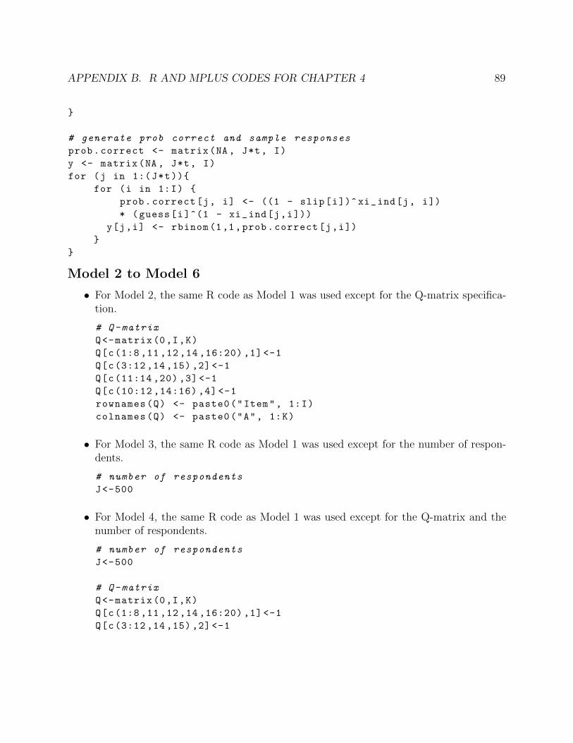
APPENDIX B. R AND MPLUS CODES FOR CHAPTER 4 89
}
# generate prob correct and sample responses
prob.correct <- matrix(NA , J*t, I)
y <- matrix(NA , J*t, I)
for (j in 1:(J*t)){
for (i in 1:I) {
prob.correct[j, i] <- ((1 - slip[i])^xi_ind[j, i])
* (guess[i]^(1 - xi_ind[j,i]))
y[j,i] <- rbinom(1,1,prob.correct[j,i])
}
}
Model 2 to Model 6
• For Model 2, the same R code as Model 1 was used except for the Q-matrix specifica-tion.
# Q-matrix
Q<-matrix(0,I,K)
Q[c(1:8 ,11 ,12 ,14 ,16:20) ,1] <-1
Q[c(3:12 ,14 ,15) ,2] <-1
Q[c(11:14 ,20) ,3] <-1
Q[c(10:12 ,14:16) ,4] <-1
rownames(Q) <- paste0("Item", 1:I)
colnames(Q) <- paste0("A", 1:K)
• For Model 3, the same R code as Model 1 was used except for the number of respon-dents.
# number of respondents
J<-500
• For Model 4, the same R code as Model 1 was used except for the Q-matrix and thenumber of respondents.
# number of respondents
J<-500
# Q-matrix
Q<-matrix(0,I,K)
Q[c(1:8 ,11 ,12 ,14 ,16:20) ,1] <-1
Q[c(3:12 ,14 ,15) ,2] <-1
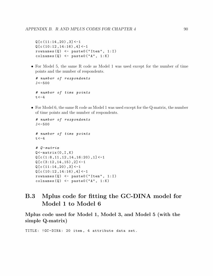
APPENDIX B. R AND MPLUS CODES FOR CHAPTER 4 90
Q[c(11:14 ,20) ,3] <-1
Q[c(10:12 ,14:16) ,4] <-1
rownames(Q) <- paste0("Item", 1:I)
colnames(Q) <- paste0("A", 1:K)
• For Model 5, the same R code as Model 1 was used except for the number of timepoints and the number of respondents.
# number of respondents
J<-500
# number of time points
t<-4
• For Model 6, the same R code as Model 1 was used except for the Q-matrix, the numberof time points and the number of respondents.
# number of respondents
J<-500
# number of time points
t<-4
# Q-matrix
Q<-matrix(0,I,K)
Q[c(1:8 ,11 ,12 ,14 ,16:20) ,1] <-1
Q[c(3:12 ,14 ,15) ,2] <-1
Q[c(11:14 ,20) ,3] <-1
Q[c(10:12 ,14:16) ,4] <-1
rownames(Q) <- paste0("Item", 1:I)
colnames(Q) <- paste0("A", 1:K)
B.3 Mplus code for fitting the GC-DINA model for
Model 1 to Model 6
Mplus code used for Model 1, Model 3, and Model 5 (with thesimple Q-matrix)
TITLE: !GC -DINA: 20 item , 4 attribute data set.
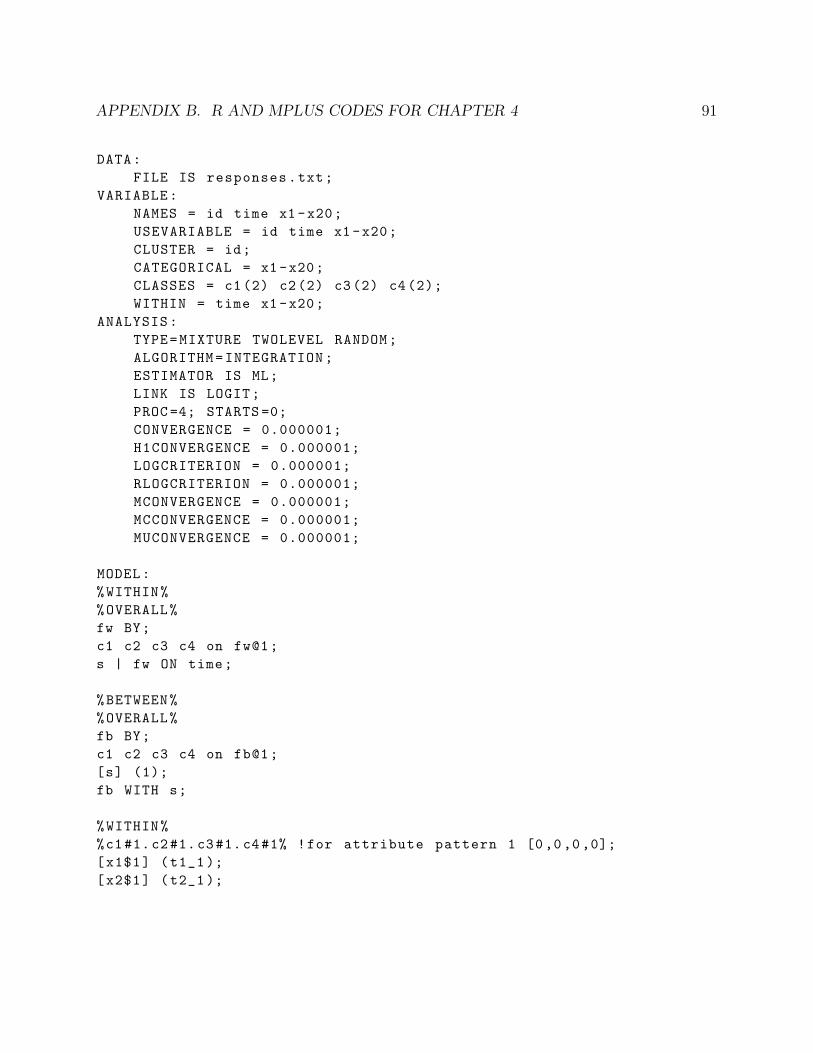
APPENDIX B. R AND MPLUS CODES FOR CHAPTER 4 91
DATA:
FILE IS responses.txt;
VARIABLE:
NAMES = id time x1-x20;
USEVARIABLE = id time x1-x20;
CLUSTER = id;
CATEGORICAL = x1-x20;
CLASSES = c1(2) c2(2) c3(2) c4(2);
WITHIN = time x1 -x20;
ANALYSIS:
TYPE=MIXTURE TWOLEVEL RANDOM;
ALGORITHM=INTEGRATION;
ESTIMATOR IS ML;
LINK IS LOGIT;
PROC =4; STARTS =0;
CONVERGENCE = 0.000001;
H1CONVERGENCE = 0.000001;
LOGCRITERION = 0.000001;
RLOGCRITERION = 0.000001;
MCONVERGENCE = 0.000001;
MCCONVERGENCE = 0.000001;
MUCONVERGENCE = 0.000001;
MODEL:
%WITHIN%
%OVERALL%
fw BY;
c1 c2 c3 c4 on fw@1;
s | fw ON time;
%BETWEEN%
%OVERALL%
fb BY;
c1 c2 c3 c4 on fb@1;
[s] (1);
fb WITH s;
%WITHIN%
%c1#1.c2#1.c3#1.c4#1% !for attribute pattern 1 [0,0,0,0];
[x1$1] (t1_1);
[x2$1] (t2_1);

APPENDIX B. R AND MPLUS CODES FOR CHAPTER 4 92
[x3$1] (t3_1);
[x4$1] (t4_1);
[x5$1] (t5_1);
[x6$1] (t6_1);
[x7$1] (t7_1);
[x8$1] (t8_1);
[x9$1] (t9_1);
[x10$1] (t10_1 );
[x11$1] (t11_1 );
[x12$1] (t12_1 );
[x13$1] (t13_1 );
[x14$1] (t14_1 );
[x15$1] (t15_1 );
[x16$1] (t16_1 );
[x17$1] (t17_1 );
[x18$1] (t18_1 );
[x19$1] (t19_1 );
[x20$1] (t20_1 );
%c1#2.c2#1.c3#1.c4#1% !for attribute pattern 2 [1,0,0,0];
[x1$1] (t1_2);
[x2$1] (t2_1);
[x3$1] (t3_1);
[x4$1] (t4_1);
[x5$1] (t5_1);
[x6$1] (t6_1);
[x7$1] (t7_1);
[x8$1] (t8_1);
[x9$1] (t9_1);
[x10$1] (t10_1 );
[x11$1] (t11_1 );
[x12$1] (t12_1 );
[x13$1] (t13_2 );
[x14$1] (t14_2 );
[x15$1] (t15_1 );
[x16$1] (t16_1 );
[x17$1] (t17_2 );
[x18$1] (t18_1 );
[x19$1] (t19_1 );
[x20$1] (t20_1 );
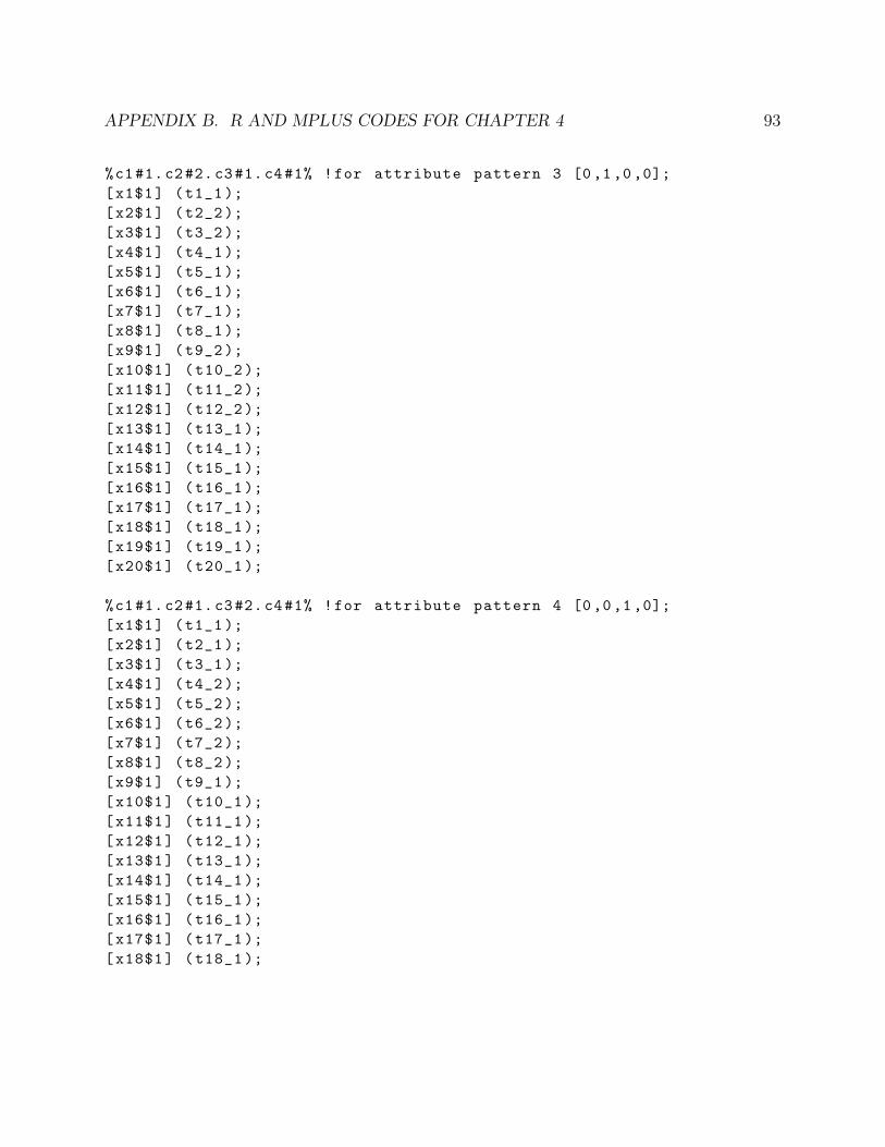
APPENDIX B. R AND MPLUS CODES FOR CHAPTER 4 93
%c1#1.c2#2.c3#1.c4#1% !for attribute pattern 3 [0,1,0,0];
[x1$1] (t1_1);
[x2$1] (t2_2);
[x3$1] (t3_2);
[x4$1] (t4_1);
[x5$1] (t5_1);
[x6$1] (t6_1);
[x7$1] (t7_1);
[x8$1] (t8_1);
[x9$1] (t9_2);
[x10$1] (t10_2 );
[x11$1] (t11_2 );
[x12$1] (t12_2 );
[x13$1] (t13_1 );
[x14$1] (t14_1 );
[x15$1] (t15_1 );
[x16$1] (t16_1 );
[x17$1] (t17_1 );
[x18$1] (t18_1 );
[x19$1] (t19_1 );
[x20$1] (t20_1 );
%c1#1.c2#1.c3#2.c4#1% !for attribute pattern 4 [0,0,1,0];
[x1$1] (t1_1);
[x2$1] (t2_1);
[x3$1] (t3_1);
[x4$1] (t4_2);
[x5$1] (t5_2);
[x6$1] (t6_2);
[x7$1] (t7_2);
[x8$1] (t8_2);
[x9$1] (t9_1);
[x10$1] (t10_1 );
[x11$1] (t11_1 );
[x12$1] (t12_1 );
[x13$1] (t13_1 );
[x14$1] (t14_1 );
[x15$1] (t15_1 );
[x16$1] (t16_1 );
[x17$1] (t17_1 );
[x18$1] (t18_1 );
APPENDIX B. R AND MPLUS CODES FOR CHAPTER 4 94
[x19$1] (t19_1 );
[x20$1] (t20_1 );
%c1#1.c2#1.c3#1.c4#2% !for attribute pattern 5 [0,0,0,1];
[x1$1] (t1_1);
[x2$1] (t2_1);
[x3$1] (t3_1);
[x4$1] (t4_1);
[x5$1] (t5_1);
[x6$1] (t6_1);
[x7$1] (t7_1);
[x8$1] (t8_1);
[x9$1] (t9_1);
[x10$1] (t10_1 );
[x11$1] (t11_1 );
[x12$1] (t12_1 );
[x13$1] (t13_1 );
[x14$1] (t14_1 );
[x15$1] (t15_2 );
[x16$1] (t16_2 );
[x17$1] (t17_1 );
[x18$1] (t18_2 );
[x19$1] (t19_2 );
[x20$1] (t20_2 );
%c1#2.c2#2.c3#1.c4#1% !for attribute pattern 6 [1,1,0,0];
[x1$1] (t1_2);
[x2$1] (t2_2);
[x3$1] (t3_2);
[x4$1] (t4_1);
[x5$1] (t5_1);
[x6$1] (t6_1);
[x7$1] (t7_1);
[x8$1] (t8_1);
[x9$1] (t9_2);
[x10$1] (t10_2 );
[x11$1] (t11_2 );
[x12$1] (t12_2 );
[x13$1] (t13_2 );
[x14$1] (t14_2 );
[x15$1] (t15_1 );
APPENDIX B. R AND MPLUS CODES FOR CHAPTER 4 95
[x16$1] (t16_1 );
[x17$1] (t17_2 );
[x18$1] (t18_1 );
[x19$1] (t19_1 );
[x20$1] (t20_1 );
%c1#2.c2#1.c3#2.c4#1% !for attribute pattern 7 [1,0,1,0];
[x1$1] (t1_2);
[x2$1] (t2_1);
[x3$1] (t3_1);
[x4$1] (t4_2);
[x5$1] (t5_2);
[x6$1] (t6_2);
[x7$1] (t7_2);
[x8$1] (t8_2);
[x9$1] (t9_1);
[x10$1] (t10_1 );
[x11$1] (t11_1 );
[x12$1] (t12_1 );
[x13$1] (t13_2 );
[x14$1] (t14_2 );
[x15$1] (t15_1 );
[x16$1] (t16_1 );
[x17$1] (t17_2 );
[x18$1] (t18_1 );
[x19$1] (t19_1 );
[x20$1] (t20_1 );
%c1#2.c2#1.c3#1.c4#2% !for attribute pattern 8 [1,0,0,1];
[x1$1] (t1_2);
[x2$1] (t2_1);
[x3$1] (t3_1);
[x4$1] (t4_1);
[x5$1] (t5_1);
[x6$1] (t6_1);
[x7$1] (t7_1);
[x8$1] (t8_1);
[x9$1] (t9_1);
[x10$1] (t10_1 );
[x11$1] (t11_1 );
[x12$1] (t12_1 );

APPENDIX B. R AND MPLUS CODES FOR CHAPTER 4 96
[x13$1] (t13_2 );
[x14$1] (t14_2 );
[x15$1] (t15_2 );
[x16$1] (t16_2 );
[x17$1] (t17_2 );
[x18$1] (t18_2 );
[x19$1] (t19_2 );
[x20$1] (t20_2 );
%c1#1.c2#2.c3#2.c4#1% !for attribute pattern 9 [0,1,1,0];
[x1$1] (t1_1);
[x2$1] (t2_2);
[x3$1] (t3_2);
[x4$1] (t4_2);
[x5$1] (t5_2);
[x6$1] (t6_2);
[x7$1] (t7_2);
[x8$1] (t8_2);
[x9$1] (t9_2);
[x10$1] (t10_2 );
[x11$1] (t11_2 );
[x12$1] (t12_2 );
[x13$1] (t13_1 );
[x14$1] (t14_1 );
[x15$1] (t15_1 );
[x16$1] (t16_1 );
[x17$1] (t17_1 );
[x18$1] (t18_1 );
[x19$1] (t19_1 );
[x20$1] (t20_1 );
%c1#1.c2#2.c3#1.c4#2% !for attribute pattern 10 [0,1,0,1];
[x1$1] (t1_1);
[x2$1] (t2_2);
[x3$1] (t3_2);
[x4$1] (t4_1);
[x5$1] (t5_1);
[x6$1] (t6_1);
[x7$1] (t7_1);
[x8$1] (t8_1);
[x9$1] (t9_2);

APPENDIX B. R AND MPLUS CODES FOR CHAPTER 4 97
[x10$1] (t10_2 );
[x11$1] (t11_2 );
[x12$1] (t12_2 );
[x13$1] (t13_1 );
[x14$1] (t14_1 );
[x15$1] (t15_2 );
[x16$1] (t16_2 );
[x17$1] (t17_1 );
[x18$1] (t18_2 );
[x19$1] (t19_2 );
[x20$1] (t20_2 );
%c1#1.c2#1.c3#2.c4#2% !for attribute pattern 11 [0,0,1,1];
[x1$1] (t1_1);
[x2$1] (t2_1);
[x3$1] (t3_1);
[x4$1] (t4_2);
[x5$1] (t5_2);
[x6$1] (t6_2);
[x7$1] (t7_2);
[x8$1] (t8_2);
[x9$1] (t9_1);
[x10$1] (t10_1 );
[x11$1] (t11_1 );
[x12$1] (t12_1 );
[x13$1] (t13_1 );
[x14$1] (t14_1 );
[x15$1] (t15_2 );
[x16$1] (t16_2 );
[x17$1] (t17_1 );
[x18$1] (t18_2 );
[x19$1] (t19_2 );
[x20$1] (t20_2 );
%c1#2.c2#2.c3#2.c4#1% !for attribute pattern 12 [1,1,1,0];
[x1$1] (t1_2);
[x2$1] (t2_2);
[x3$1] (t3_2);
[x4$1] (t4_2);
[x5$1] (t5_2);
[x6$1] (t6_2);

APPENDIX B. R AND MPLUS CODES FOR CHAPTER 4 98
[x7$1] (t7_2);
[x8$1] (t8_2);
[x9$1] (t9_2);
[x10$1] (t10_2 );
[x11$1] (t11_2 );
[x12$1] (t12_2 );
[x13$1] (t13_2 );
[x14$1] (t14_2 );
[x15$1] (t15_1 );
[x16$1] (t16_1 );
[x17$1] (t17_2 );
[x18$1] (t18_1 );
[x19$1] (t19_1 );
[x20$1] (t20_1 );
%c1#2.c2#2.c3#1.c4#2% !for attribute pattern 13 [1,1,0,1];
[x1$1] (t1_2);
[x2$1] (t2_2);
[x3$1] (t3_2);
[x4$1] (t4_1);
[x5$1] (t5_1);
[x6$1] (t6_1);
[x7$1] (t7_1);
[x8$1] (t8_1);
[x9$1] (t9_2);
[x10$1] (t10_2 );
[x11$1] (t11_2 );
[x12$1] (t12_2 );
[x13$1] (t13_2 );
[x14$1] (t14_2 );
[x15$1] (t15_2 );
[x16$1] (t16_2 );
[x17$1] (t17_2 );
[x18$1] (t18_2 );
[x19$1] (t19_2 );
[x20$1] (t20_2 );
%c1#2.c2#1.c3#2.c4#2% !for attribute pattern 14 [1,0,1,1];
[x1$1] (t1_2);
[x2$1] (t2_1);
[x3$1] (t3_1);
APPENDIX B. R AND MPLUS CODES FOR CHAPTER 4 99
[x4$1] (t4_2);
[x5$1] (t5_2);
[x6$1] (t6_2);
[x7$1] (t7_2);
[x8$1] (t8_2);
[x9$1] (t9_1);
[x10$1] (t10_1 );
[x11$1] (t11_1 );
[x12$1] (t12_1 );
[x13$1] (t13_2 );
[x14$1] (t14_2 );
[x15$1] (t15_2 );
[x16$1] (t16_2 );
[x17$1] (t17_2 );
[x18$1] (t18_2 );
[x19$1] (t19_2 );
[x20$1] (t20_2 );
%c1#1.c2#2.c3#2.c4#2% !for attribute pattern 15 [0,1,1,1];
[x1$1] (t1_1);
[x2$1] (t2_2);
[x3$1] (t3_2);
[x4$1] (t4_2);
[x5$1] (t5_2);
[x6$1] (t6_2);
[x7$1] (t7_2);
[x8$1] (t8_2);
[x9$1] (t9_2);
[x10$1] (t10_2 );
[x11$1] (t11_2 );
[x12$1] (t12_2 );
[x13$1] (t13_1 );
[x14$1] (t14_1 );
[x15$1] (t15_2 );
[x16$1] (t16_2 );
[x17$1] (t17_1 );
[x18$1] (t18_2 );
[x19$1] (t19_2 );
[x20$1] (t20_2 );
%c1#2.c2#2.c3#2.c4#2% !for attribute pattern 16 [1,1,1,1];
APPENDIX B. R AND MPLUS CODES FOR CHAPTER 4 100
[x1$1] (t1_2);
[x2$1] (t2_2);
[x3$1] (t3_2);
[x4$1] (t4_2);
[x5$1] (t5_2);
[x6$1] (t6_2);
[x7$1] (t7_2);
[x8$1] (t8_2);
[x9$1] (t9_2);
[x10$1] (t10_2 );
[x11$1] (t11_2 );
[x12$1] (t12_2 );
[x13$1] (t13_2 );
[x14$1] (t14_2 );
[x15$1] (t15_2 );
[x16$1] (t16_2 );
[x17$1] (t17_2 );
[x18$1] (t18_2 );
[x19$1] (t19_2 );
[x20$1] (t20_2 );
MODEL CONSTRAINT:
!ITEM 1:
NEW(l1_0 l1_e);
t1_1=-(l1_0);
t1_2=-(l1_0+l1_e);
l1_e >0;
!ITEM 2:
NEW(l2_0 l2_e);
t2_1=-(l2_0);
t2_2=-(l2_0+l2_e);
l2_e >0;
!ITEM 3:
NEW(l3_0 l3_e);
t3_1=-(l3_0);
t3_2=-(l3_0+l3_e);
l3_e >0;
!ITEM 4:
APPENDIX B. R AND MPLUS CODES FOR CHAPTER 4 101
NEW(l4_0 l4_e);
t4_1=-(l4_0);
t4_2=-(l4_0+l4_e);
l4_e >0;
!ITEM 5:
NEW(l5_0 l5_e);
t5_1=-(l5_0);
t5_2=-(l5_0+l5_e);
l5_e >0;
!ITEM 6:
NEW(l6_0 l6_e);
t6_1=-(l6_0);
t6_2=-(l6_0+l6_e);
l6_e >0;
!ITEM 7:
NEW(l7_0 l7_e);
t7_1=-(l7_0);
t7_2=-(l7_0+l7_e);
l7_e >0;
!ITEM 8:
NEW(l8_0 l8_e);
t8_1=-(l8_0);
t8_2=-(l8_0+l8_e);
l8_e >0;
!ITEM 9:
NEW(l9_0 l9_e);
t9_1=-(l9_0);
t9_2=-(l9_0+l9_e);
l9_e >0;
!ITEM 10:
NEW(l10_0 l10_e);
t10_1=-(l10_0);
t10_2=-(l10_0+l10_e);
l10_e >0;
APPENDIX B. R AND MPLUS CODES FOR CHAPTER 4 102
!ITEM 11:
NEW(l11_0 l11_e);
t11_1=-(l11_0);
t11_2=-(l11_0+l11_e);
l11_e >0;
!ITEM 12:
NEW(l12_0 l12_e);
t12_1=-(l12_0);
t12_2=-(l12_0+l12_e);
l12_e >0;
!ITEM 13:
NEW(l13_0 l13_e);
t13_1=-(l13_0);
t13_2=-(l13_0+l13_e);
l13_e >0;
!ITEM 14:
NEW(l14_0 l14_e);
t14_1=-(l14_0);
t14_2=-(l14_0+l14_e);
l14_e >0;
!ITEM 15:
NEW(l15_0 l15_e);
t15_1=-(l15_0);
t15_2=-(l15_0+l15_e);
l15_e >0;
!ITEM 16:
NEW(l16_0 l16_e);
t16_1=-(l16_0);
t16_2=-(l16_0+l16_e);
l16_e >0;
!ITEM 17:
NEW(l17_0 l17_e);
t17_1=-(l17_0);
t17_2=-(l17_0+l17_e);
APPENDIX B. R AND MPLUS CODES FOR CHAPTER 4 103
l17_e >0;
!ITEM 18:
NEW(l18_0 l18_e);
t18_1=-(l18_0);
t18_2=-(l18_0+l18_e);
l18_e >0;
!ITEM 19:
NEW(l19_0 l19_e);
t19_1=-(l19_0);
t19_2=-(l19_0+l19_e);
l19_e >0;
!ITEM 20:
NEW(l20_0 l20_e);
t20_1=-(l20_0);
t20_2=-(l20_0+l20_e);
l20_e >0;
OUTPUT:
TECH1 TECH3 TECH4 TECH5 TECH8;
SAVEDATA:
FORMAT IS f10 .5;
FILE IS predicted.dat;
SAVE = CPROBABILITIES FSCORES ;;
Mplus code used for Model 2, Model 4, and Model 6 (with thecomplex Q-matrix)
TITLE: !GC -DINA: 20 item , 4 attribute data set.
DATA:
FILE IS responses.txt;
VARIABLE:
NAMES = id time x1-x20;
USEVARIABLE = id time x1-x20;
CLUSTER = id;
CATEGORICAL = x1-x20;
CLASSES = c1(2) c2(2) c3(2) c4(2);
WITHIN = time x1 -x20;
ANALYSIS:
APPENDIX B. R AND MPLUS CODES FOR CHAPTER 4 104
TYPE=MIXTURE TWOLEVEL RANDOM;
ALGORITHM=INTEGRATION;
ESTIMATOR IS ML;
LINK IS LOGIT;
PROC =4; STARTS =0;
CONVERGENCE = 0.000001;
H1CONVERGENCE = 0.000001;
LOGCRITERION = 0.000001;
RLOGCRITERION = 0.000001;
MCONVERGENCE = 0.000001;
MCCONVERGENCE = 0.000001;
MUCONVERGENCE = 0.000001;
MODEL:
%WITHIN%
%OVERALL%
fw BY;
c1 c2 c3 c4 on fw@1;
s | fw ON time;
%BETWEEN%
%OVERALL%
fb BY;
c1 c2 c3 c4 on fb@1;
[s] (1);
fb WITH s;
%WITHIN%
%c1#1.c2#1.c3#1.c4#1% !for attribute pattern 1 [0,0,0,0];
[x1$1] (t1_1);
[x2$1] (t2_1);
[x3$1] (t3_1);
[x4$1] (t4_1);
[x5$1] (t5_1);
[x6$1] (t6_1);
[x7$1] (t7_1);
[x8$1] (t8_1);
[x9$1] (t9_1);
[x10$1] (t10_1 );
[x11$1] (t11_1 );
[x12$1] (t12_1 );
APPENDIX B. R AND MPLUS CODES FOR CHAPTER 4 105
[x13$1] (t13_1 );
[x14$1] (t14_1 );
[x15$1] (t15_1 );
[x16$1] (t16_1 );
[x17$1] (t17_1 );
[x18$1] (t18_1 );
[x19$1] (t19_1 );
[x20$1] (t20_1 );
%c1#2.c2#1.c3#1.c4#1% !for attribute pattern 2 [1,0,0,0];
[x1$1] (t1_2);
[x2$1] (t2_2);
[x3$1] (t3_1);
[x4$1] (t4_1);
[x5$1] (t5_1);
[x6$1] (t6_1);
[x7$1] (t7_1);
[x8$1] (t8_1);
[x9$1] (t9_1);
[x10$1] (t10_1 );
[x11$1] (t11_1 );
[x12$1] (t12_1 );
[x13$1] (t13_1 );
[x14$1] (t14_1 );
[x15$1] (t15_1 );
[x16$1] (t16_1 );
[x17$1] (t17_2 );
[x18$1] (t18_2 );
[x19$1] (t19_2 );
[x20$1] (t20_1 );
%c1#1.c2#2.c3#1.c4#1% !for attribute pattern 3 [0,1,0,0];
[x1$1] (t1_1);
[x2$1] (t2_1);
[x3$1] (t3_1);
[x4$1] (t4_1);
[x5$1] (t5_1);
[x6$1] (t6_1);
[x7$1] (t7_1);
[x8$1] (t8_1);
APPENDIX B. R AND MPLUS CODES FOR CHAPTER 4 106
[x9$1] (t9_2);
[x10$1] (t10_1 );
[x11$1] (t11_1 );
[x12$1] (t12_1 );
[x13$1] (t13_1 );
[x14$1] (t14_1 );
[x15$1] (t15_1 );
[x16$1] (t16_1 );
[x17$1] (t17_1 );
[x18$1] (t18_1 );
[x19$1] (t19_1 );
[x20$1] (t20_1 );
%c1#1.c2#1.c3#2.c4#1% !for attribute pattern 4 [0,0,1,0];
[x1$1] (t1_1);
[x2$1] (t2_1);
[x3$1] (t3_1);
[x4$1] (t4_1);
[x5$1] (t5_1);
[x6$1] (t6_1);
[x7$1] (t7_1);
[x8$1] (t8_1);
[x9$1] (t9_1);
[x10$1] (t10_1 );
[x11$1] (t11_1 );
[x12$1] (t12_1 );
[x13$1] (t13_2 );
[x14$1] (t14_1 );
[x15$1] (t15_1 );
[x16$1] (t16_1 );
[x17$1] (t17_1 );
[x18$1] (t18_1 );
[x19$1] (t19_1 );
[x20$1] (t20_1 );
%c1#1.c2#1.c3#1.c4#2% !for attribute pattern 5 [0,0,0,1];
[x1$1] (t1_1);
[x2$1] (t2_1);
[x3$1] (t3_1);

APPENDIX B. R AND MPLUS CODES FOR CHAPTER 4 107
[x4$1] (t4_1);
[x5$1] (t5_1);
[x6$1] (t6_1);
[x7$1] (t7_1);
[x8$1] (t8_1);
[x9$1] (t9_1);
[x10$1] (t10_1 );
[x11$1] (t11_1 );
[x12$1] (t12_1 );
[x13$1] (t13_1 );
[x14$1] (t14_1 );
[x15$1] (t15_1 );
[x16$1] (t16_1 );
[x17$1] (t17_1 );
[x18$1] (t18_1 );
[x19$1] (t19_1 );
[x20$1] (t20_1 );
%c1#2.c2#2.c3#1.c4#1% !for attribute pattern 6 [1,1,0,0];
[x1$1] (t1_2);
[x2$1] (t2_2);
[x3$1] (t3_2);
[x4$1] (t4_2);
[x5$1] (t5_2);
[x6$1] (t6_2);
[x7$1] (t7_2);
[x8$1] (t8_2);
[x9$1] (t9_2);
[x10$1] (t10_1 );
[x11$1] (t11_1 );
[x12$1] (t12_1 );
[x13$1] (t13_1 );
[x14$1] (t14_1 );
[x15$1] (t15_1 );
[x16$1] (t16_1 );
[x17$1] (t17_2 );
[x18$1] (t18_2 );
[x19$1] (t19_2 );
[x20$1] (t20_1 );

APPENDIX B. R AND MPLUS CODES FOR CHAPTER 4 108
%c1#2.c2#1.c3#2.c4#1% !for attribute pattern 7 [1,0,1,0];
[x1$1] (t1_2);
[x2$1] (t2_2);
[x3$1] (t3_1);
[x4$1] (t4_1);
[x5$1] (t5_1);
[x6$1] (t6_1);
[x7$1] (t7_1);
[x8$1] (t8_1);
[x9$1] (t9_1);
[x10$1] (t10_1 );
[x11$1] (t11_1 );
[x12$1] (t12_1 );
[x13$1] (t13_2 );
[x14$1] (t14_1 );
[x15$1] (t15_1 );
[x16$1] (t16_1 );
[x17$1] (t17_2 );
[x18$1] (t18_2 );
[x19$1] (t19_2 );
[x20$1] (t20_2 );
%c1#2.c2#1.c3#1.c4#2% !for attribute pattern 8 [1,0,0,1];
[x1$1] (t1_2);
[x2$1] (t2_2);
[x3$1] (t3_1);
[x4$1] (t4_1);
[x5$1] (t5_1);
[x6$1] (t6_1);
[x7$1] (t7_1);
[x8$1] (t8_1);
[x9$1] (t9_1);
[x10$1] (t10_1 );
[x11$1] (t11_1 );
[x12$1] (t12_1 );
[x13$1] (t13_1 );
[x14$1] (t14_1 );
[x15$1] (t15_1 );
[x16$1] (t16_2 );
[x17$1] (t17_2 );
[x18$1] (t18_2 );
APPENDIX B. R AND MPLUS CODES FOR CHAPTER 4 109
[x19$1] (t19_2 );
[x20$1] (t20_1 );
%c1#1.c2#2.c3#2.c4#1% !for attribute pattern 9 [0,1,1,0];
[x1$1] (t1_1);
[x2$1] (t2_1);
[x3$1] (t3_1);
[x4$1] (t4_1);
[x5$1] (t5_1);
[x6$1] (t6_1);
[x7$1] (t7_1);
[x8$1] (t8_1);
[x9$1] (t9_2);
[x10$1] (t10_1 );
[x11$1] (t11_1 );
[x12$1] (t12_1 );
[x13$1] (t13_2 );
[x14$1] (t14_1 );
[x15$1] (t15_1 );
[x16$1] (t16_1 );
[x17$1] (t17_1 );
[x18$1] (t18_1 );
[x19$1] (t19_1 );
[x20$1] (t20_1 );
%c1#1.c2#2.c3#1.c4#2% !for attribute pattern 10 [0,1,0,1];
[x1$1] (t1_1);
[x2$1] (t2_1);
[x3$1] (t3_1);
[x4$1] (t4_1);
[x5$1] (t5_1);
[x6$1] (t6_1);
[x7$1] (t7_1);
[x8$1] (t8_1);
[x9$1] (t9_2);
[x10$1] (t10_2 );
[x11$1] (t11_1 );
[x12$1] (t12_1 );
[x13$1] (t13_1 );
APPENDIX B. R AND MPLUS CODES FOR CHAPTER 4 110
[x14$1] (t14_1 );
[x15$1] (t15_2 );
[x16$1] (t16_1 );
[x17$1] (t17_1 );
[x18$1] (t18_1 );
[x19$1] (t19_1 );
[x20$1] (t20_1 );
%c1#1.c2#1.c3#2.c4#2% !for attribute pattern 11 [0,0,1,1];
[x1$1] (t1_1);
[x2$1] (t2_1);
[x3$1] (t3_1);
[x4$1] (t4_1);
[x5$1] (t5_1);
[x6$1] (t6_1);
[x7$1] (t7_1);
[x8$1] (t8_1);
[x9$1] (t9_1);
[x10$1] (t10_1 );
[x11$1] (t11_1 );
[x12$1] (t12_1 );
[x13$1] (t13_2 );
[x14$1] (t14_1 );
[x15$1] (t15_1 );
[x16$1] (t16_1 );
[x17$1] (t17_1 );
[x18$1] (t18_1 );
[x19$1] (t19_1 );
[x20$1] (t20_1 );
%c1#2.c2#2.c3#2.c4#1% !for attribute pattern 12 [1,1,1,0];
[x1$1] (t1_2);
[x2$1] (t2_2);
[x3$1] (t3_2);
[x4$1] (t4_2);
[x5$1] (t5_2);
[x6$1] (t6_2);
[x7$1] (t7_2);
[x8$1] (t8_2);

APPENDIX B. R AND MPLUS CODES FOR CHAPTER 4 111
[x9$1] (t9_2);
[x10$1] (t10_1 );
[x11$1] (t11_1 );
[x12$1] (t12_1 );
[x13$1] (t13_2 );
[x14$1] (t14_1 );
[x15$1] (t15_1 );
[x16$1] (t16_1 );
[x17$1] (t17_2 );
[x18$1] (t18_2 );
[x19$1] (t19_2 );
[x20$1] (t20_2 );
%c1#2.c2#2.c3#1.c4#2% !for attribute pattern 13 [1,1,0,1];
[x1$1] (t1_2);
[x2$1] (t2_2);
[x3$1] (t3_2);
[x4$1] (t4_2);
[x5$1] (t5_2);
[x6$1] (t6_2);
[x7$1] (t7_2);
[x8$1] (t8_2);
[x9$1] (t9_2);
[x10$1] (t10_2 );
[x11$1] (t11_1 );
[x12$1] (t12_1 );
[x13$1] (t13_1 );
[x14$1] (t14_1 );
[x15$1] (t15_2 );
[x16$1] (t16_2 );
[x17$1] (t17_2 );
[x18$1] (t18_2 );
[x19$1] (t19_2 );
[x20$1] (t20_1 );
%c1#2.c2#1.c3#2.c4#2% !for attribute pattern 14 [1,0,1,1];
[x1$1] (t1_2);
[x2$1] (t2_2);
[x3$1] (t3_1);
APPENDIX B. R AND MPLUS CODES FOR CHAPTER 4 112
[x4$1] (t4_1);
[x5$1] (t5_1);
[x6$1] (t6_1);
[x7$1] (t7_1);
[x8$1] (t8_1);
[x9$1] (t9_1);
[x10$1] (t10_1 );
[x11$1] (t11_1 );
[x12$1] (t12_1 );
[x13$1] (t13_2 );
[x14$1] (t14_1 );
[x15$1] (t15_1 );
[x16$1] (t16_2 );
[x17$1] (t17_2 );
[x18$1] (t18_2 );
[x19$1] (t19_2 );
[x20$1] (t20_2 );
%c1#1.c2#2.c3#2.c4#2% !for attribute pattern 15 [0,1,1,1];
[x1$1] (t1_1);
[x2$1] (t2_1);
[x3$1] (t3_1);
[x4$1] (t4_1);
[x5$1] (t5_1);
[x6$1] (t6_1);
[x7$1] (t7_1);
[x8$1] (t8_1);
[x9$1] (t9_2);
[x10$1] (t10_2 );
[x11$1] (t11_1 );
[x12$1] (t12_1 );
[x13$1] (t13_2 );
[x14$1] (t14_1 );
[x15$1] (t15_2 );
[x16$1] (t16_1 );
[x17$1] (t17_1 );
[x18$1] (t18_1 );
[x19$1] (t19_1 );
[x20$1] (t20_1 );
APPENDIX B. R AND MPLUS CODES FOR CHAPTER 4 113
%c1#2.c2#2.c3#2.c4#2% !for attribute pattern 16 [1,1,1,1];
[x1$1] (t1_2);
[x2$1] (t2_2);
[x3$1] (t3_2);
[x4$1] (t4_2);
[x5$1] (t5_2);
[x6$1] (t6_2);
[x7$1] (t7_2);
[x8$1] (t8_2);
[x9$1] (t9_2);
[x10$1] (t10_2 );
[x11$1] (t11_2 );
[x12$1] (t12_2 );
[x13$1] (t13_2 );
[x14$1] (t14_2 );
[x15$1] (t15_2 );
[x16$1] (t16_2 );
[x17$1] (t17_2 );
[x18$1] (t18_2 );
[x19$1] (t19_2 );
[x20$1] (t20_2 );
MODEL CONSTRAINT:
!ITEM 1:
NEW(l1_0 l1_e);
t1_1=-(l1_0);
t1_2=-(l1_0+l1_e);
l1_e >0;
!ITEM 2:
NEW(l2_0 l2_e);
t2_1=-(l2_0);
t2_2=-(l2_0+l2_e);
l2_e >0;
!ITEM 3:
NEW(l3_0 l3_e);
t3_1=-(l3_0);
t3_2=-(l3_0+l3_e);
l3_e >0;
APPENDIX B. R AND MPLUS CODES FOR CHAPTER 4 114
!ITEM 4:
NEW(l4_0 l4_e);
t4_1=-(l4_0);
t4_2=-(l4_0+l4_e);
l4_e >0;
!ITEM 5:
NEW(l5_0 l5_e);
t5_1=-(l5_0);
t5_2=-(l5_0+l5_e);
l5_e >0;
!ITEM 6:
NEW(l6_0 l6_e);
t6_1=-(l6_0);
t6_2=-(l6_0+l6_e);
l6_e >0;
!ITEM 7:
NEW(l7_0 l7_e);
t7_1=-(l7_0);
t7_2=-(l7_0+l7_e);
l7_e >0;
!ITEM 8:
NEW(l8_0 l8_e);
t8_1=-(l8_0);
t8_2=-(l8_0+l8_e);
l8_e >0;
!ITEM 9:
NEW(l9_0 l9_e);
t9_1=-(l9_0);
t9_2=-(l9_0+l9_e);
l9_e >0;
!ITEM 10:
NEW(l10_0 l10_e);
t10_1=-(l10_0);
APPENDIX B. R AND MPLUS CODES FOR CHAPTER 4 115
t10_2=-(l10_0+l10_e);
l10_e >0;
!ITEM 11:
NEW(l11_0 l11_e);
t11_1=-(l11_0);
t11_2=-(l11_0+l11_e);
l11_e >0;
!ITEM 12:
NEW(l12_0 l12_e);
t12_1=-(l12_0);
t12_2=-(l12_0+l12_e);
l12_e >0;
!ITEM 13:
NEW(l13_0 l13_e);
t13_1=-(l13_0);
t13_2=-(l13_0+l13_e);
l13_e >0;
!ITEM 14:
NEW(l14_0 l14_e);
t14_1=-(l14_0);
t14_2=-(l14_0+l14_e);
l14_e >0;
!ITEM 15:
NEW(l15_0 l15_e);
t15_1=-(l15_0);
t15_2=-(l15_0+l15_e);
l15_e >0;
!ITEM 16:
NEW(l16_0 l16_e);
t16_1=-(l16_0);
t16_2=-(l16_0+l16_e);
l16_e >0;
!ITEM 17:
NEW(l17_0 l17_e);
APPENDIX B. R AND MPLUS CODES FOR CHAPTER 4 116
t17_1=-(l17_0);
t17_2=-(l17_0+l17_e);
l17_e >0;
!ITEM 18:
NEW(l18_0 l18_e);
t18_1=-(l18_0);
t18_2=-(l18_0+l18_e);
l18_e >0;
!ITEM 19:
NEW(l19_0 l19_e);
t19_1=-(l19_0);
t19_2=-(l19_0+l19_e);
l19_e >0;
!ITEM 20:
NEW(l20_0 l20_e);
t20_1=-(l20_0);
t20_2=-(l20_0+l20_e);
l20_e >0;
OUTPUT:
TECH1 TECH3 TECH4 TECH5 TECH8;
SAVEDATA:
FORMAT IS f10 .5;
FILE IS predicted.dat;
SAVE = CPROBABILITIES FSCORES ;;
B.4 R code generating data for simulation study 2
# load required packages
library(MASS)
library(boot)
# number of respondents
J<-1000
# number of items
I<-20
# number of skills
K<-4
APPENDIX B. R AND MPLUS CODES FOR CHAPTER 4 117
# Q-matrix
Q <- t(matrix(c(1,0,0,0,0,1,0,0,0,1,0,0,0,0,1,0,0,0,1,0,0,0,1,0,
0,0,1,0,0,0,1,0,0,1,0,0,0,1,0,0,0,1,0,0,0,1,0,0,1,0,0,0,1,
0,0,0,0,0,0,1,0,0,0,1,1,0,0,0,0,0,0,1,0,0,0,1,0,0,0,1),K,I))
rownames(Q) <- paste0("Item", 1:I)
colnames(Q) <- paste0("A", 1:K)
# skill profile patterns
alpha_patt <- as.matrix(expand.grid(c(0,1),c(0,1),c(0,1),c(0 ,1)))
colnames(alpha_patt) <- paste0("A", 1:4)
alpha_patt
# slip and guess
slip <- c(0.192 ,0.260 ,0.119 ,0.291 ,0.143 ,0.182 ,0.237 ,0.209 ,0.134 ,
0.241 ,0.238 ,0.206 ,0.279 ,0.164 , 0.266 ,0.256 ,0.118 ,0.291 ,0.210 ,0.264)
guess <- c(0.201 ,0.242 ,0.263 ,0.122 ,0.230 ,0.186 ,0.119 ,0.117 ,0.174 ,
0.205 ,0.274 ,0.123 ,0.265 ,0.278 ,0.293 ,0.233 ,0.133 ,0.165 ,0.150 ,0.283)
# generate higher -order latent traits at two time points
set.seed (1234)
theta <- mvrnorm(n=J,mu=c(0,0.3), Sigma=matrix(c(1,.8,.8,1),2,2))
# structural model parameters
lambda0 <- c(1.51, -1.42, -0.66, 0.5)
# generate true skill mastery profiles and sample responses
resp <-array(NA , dim=c(J,I,2))
A_all <-array(NA , dim=c(J,K,2))
for (t in 1:2){
# find the prob of respondent j having skill k
eta.jk <- matrix(0, J, K)
for (j in 1:J) {
for (k in 1:K) {
eta.jk[j, k]
<- exp(theta[j,t] + lambda0[k])/(1 + exp(theta[j,t] + lambda0[k]))
}
}
# generate a respondent ’s true skill profile
APPENDIX B. R AND MPLUS CODES FOR CHAPTER 4 118
A <- matrix(0, J, K)
for (j in 1:J) {
for (k in 1:K) {
A[j, k] <- rbinom(1, 1, eta.jk[j, k])
}
}
# calculate if respondents have all skills needed for each item
xi_ind <- matrix(0, J, I)
for (j in 1:J) {
for (i in 1:I) {
xi_ind[j, i] <- prod(A[j, ]^Q[i, ])
}
}
# generate prob correct and sample responses
prob.correct <- matrix(0, J, I)
y <- matrix(0, J, I)
for (j in 1:J) {
for (i in 1:I) {
prob.correct[j, i] <- ((1 - slip[i])^xi_ind[j, i])
* (guess[i]^(1 - xi_ind[j, i]))
y[j, i] <- rbinom(1, 1, prob.correct[j, i])
}
}
A_all[,,t]<-A
resp[,,t]<-y
}
skill_data <-cbind(A_all[,,1],A_all[,,2])
resp_data <-cbind(resp[,,1],resp[,,2])
B.5 Mplus code for fitting the GC-DINA in
simulation study 2
TITLE: !GC -DINA model for T=2
DATA:
FILE IS responses_t2.txt;
APPENDIX B. R AND MPLUS CODES FOR CHAPTER 4 119
VARIABLE:
NAMES = x1 -x20 y1 -y20; !list of variables in input file
USEVARIABLE = x1-x20 y1-y20;
CATEGORICAL = x1-x20 y1-y20;
CLASSES = c1(2) c2(2) c3(2) c4(2) c5(2) c6(2) c7(2) c8(2);
ANALYSIS:
TYPE=MIXTURE;
STARTS =0;
ALGORITHM=INTEGRATION;
MODEL:
%OVERALL%
f1 BY;
f2 BY;
c1 c2 c3 c4 ON f1@1;
c5 c6 c7 c8 ON f2@1;
[f1@0];
[f2 *0.5];
f1*1;
f2*1;
f1 -f2 WITH f1 -f2;
[c1#1] (inter1 );
[c2#1] (inter2 );
[c3#1] (inter3 );
[c4#1] (inter4 );
[c5#1] (inter1 );
[c6#1] (inter2 );
[c7#1] (inter3 );
[c8#1] (inter4 );
MODEL c1.c2.c3.c4:
%c1#1.c2#1.c3#1.c4#1% !for attribute pattern 1 [0,0,0,0];
[x1$1] (t1_1);
[x2$1] (t2_1);
[x3$1] (t3_1);
[x4$1] (t4_1);
[x5$1] (t5_1);
[x6$1] (t6_1);
[x7$1] (t7_1);
[x8$1] (t8_1);
APPENDIX B. R AND MPLUS CODES FOR CHAPTER 4 120
[x9$1] (t9_1);
[x10$1] (t10_1 );
[x11$1] (t11_1 );
[x12$1] (t12_1 );
[x13$1] (t13_1 );
[x14$1] (t14_1 );
[x15$1] (t15_1 );
[x16$1] (t16_1 );
[x17$1] (t17_1 );
[x18$1] (t18_1 );
[x19$1] (t19_1 );
[x20$1] (t20_1 );
%c1#2.c2#1.c3#1.c4#1% !for attribute pattern 2 [1,0,0,0];
[x1$1] (t1_2);
[x2$1] (t2_1);
[x3$1] (t3_1);
[x4$1] (t4_1);
[x5$1] (t5_1);
[x6$1] (t6_1);
[x7$1] (t7_1);
[x8$1] (t8_1);
[x9$1] (t9_1);
[x10$1] (t10_1 );
[x11$1] (t11_1 );
[x12$1] (t12_1 );
[x13$1] (t13_2 );
[x14$1] (t14_2 );
[x15$1] (t15_1 );
[x16$1] (t16_1 );
[x17$1] (t17_2 );
[x18$1] (t18_1 );
[x19$1] (t19_1 );
[x20$1] (t20_1 );
%c1#1.c2#2.c3#1.c4#1% !for attribute pattern 3 [0,1,0,0];
[x1$1] (t1_1);
[x2$1] (t2_2);
[x3$1] (t3_2);
[x4$1] (t4_1);
[x5$1] (t5_1);

APPENDIX B. R AND MPLUS CODES FOR CHAPTER 4 121
[x6$1] (t6_1);
[x7$1] (t7_1);
[x8$1] (t8_1);
[x9$1] (t9_2);
[x10$1] (t10_2 );
[x11$1] (t11_2 );
[x12$1] (t12_2 );
[x13$1] (t13_1 );
[x14$1] (t14_1 );
[x15$1] (t15_1 );
[x16$1] (t16_1 );
[x17$1] (t17_1 );
[x18$1] (t18_1 );
[x19$1] (t19_1 );
[x20$1] (t20_1 );
%c1#1.c2#1.c3#2.c4#1% !for attribute pattern 4 [0,0,1,0];
[x1$1] (t1_1);
[x2$1] (t2_1);
[x3$1] (t3_1);
[x4$1] (t4_2);
[x5$1] (t5_2);
[x6$1] (t6_2);
[x7$1] (t7_2);
[x8$1] (t8_2);
[x9$1] (t9_1);
[x10$1] (t10_1 );
[x11$1] (t11_1 );
[x12$1] (t12_1 );
[x13$1] (t13_1 );
[x14$1] (t14_1 );
[x15$1] (t15_1 );
[x16$1] (t16_1 );
[x17$1] (t17_1 );
[x18$1] (t18_1 );
[x19$1] (t19_1 );
[x20$1] (t20_1 );
%c1#1.c2#1.c3#1.c4#2% !for attribute pattern 5 [0,0,0,1];
[x1$1] (t1_1);
[x2$1] (t2_1);
APPENDIX B. R AND MPLUS CODES FOR CHAPTER 4 122
[x3$1] (t3_1);
[x4$1] (t4_1);
[x5$1] (t5_1);
[x6$1] (t6_1);
[x7$1] (t7_1);
[x8$1] (t8_1);
[x9$1] (t9_1);
[x10$1] (t10_1 );
[x11$1] (t11_1 );
[x12$1] (t12_1 );
[x13$1] (t13_1 );
[x14$1] (t14_1 );
[x15$1] (t15_2 );
[x16$1] (t16_2 );
[x17$1] (t17_1 );
[x18$1] (t18_2 );
[x19$1] (t19_2 );
[x20$1] (t20_2 );
%c1#2.c2#2.c3#1.c4#1% !for attribute pattern 6 [1,1,0,0];
[x1$1] (t1_2);
[x2$1] (t2_2);
[x3$1] (t3_2);
[x4$1] (t4_1);
[x5$1] (t5_1);
[x6$1] (t6_1);
[x7$1] (t7_1);
[x8$1] (t8_1);
[x9$1] (t9_2);
[x10$1] (t10_2 );
[x11$1] (t11_2 );
[x12$1] (t12_2 );
[x13$1] (t13_2 );
[x14$1] (t14_2 );
[x15$1] (t15_1 );
[x16$1] (t16_1 );
[x17$1] (t17_2 );
[x18$1] (t18_1 );
[x19$1] (t19_1 );
[x20$1] (t20_1 );
APPENDIX B. R AND MPLUS CODES FOR CHAPTER 4 123
%c1#2.c2#1.c3#2.c4#1% !for attribute pattern 7 [1,0,1,0];
[x1$1] (t1_2);
[x2$1] (t2_1);
[x3$1] (t3_1);
[x4$1] (t4_2);
[x5$1] (t5_2);
[x6$1] (t6_2);
[x7$1] (t7_2);
[x8$1] (t8_2);
[x9$1] (t9_1);
[x10$1] (t10_1 );
[x11$1] (t11_1 );
[x12$1] (t12_1 );
[x13$1] (t13_2 );
[x14$1] (t14_2 );
[x15$1] (t15_1 );
[x16$1] (t16_1 );
[x17$1] (t17_2 );
[x18$1] (t18_1 );
[x19$1] (t19_1 );
[x20$1] (t20_1 );
%c1#2.c2#1.c3#1.c4#2% !for attribute pattern 8 [1,0,0,1];
[x1$1] (t1_2);
[x2$1] (t2_1);
[x3$1] (t3_1);
[x4$1] (t4_1);
[x5$1] (t5_1);
[x6$1] (t6_1);
[x7$1] (t7_1);
[x8$1] (t8_1);
[x9$1] (t9_1);
[x10$1] (t10_1 );
[x11$1] (t11_1 );
[x12$1] (t12_1 );
[x13$1] (t13_2 );
[x14$1] (t14_2 );
[x15$1] (t15_2 );
[x16$1] (t16_2 );
[x17$1] (t17_2 );
[x18$1] (t18_2 );

APPENDIX B. R AND MPLUS CODES FOR CHAPTER 4 124
[x19$1] (t19_2 );
[x20$1] (t20_2 );
%c1#1.c2#2.c3#2.c4#1% !for attribute pattern 9 [0,1,1,0];
[x1$1] (t1_1);
[x2$1] (t2_2);
[x3$1] (t3_2);
[x4$1] (t4_2);
[x5$1] (t5_2);
[x6$1] (t6_2);
[x7$1] (t7_2);
[x8$1] (t8_2);
[x9$1] (t9_2);
[x10$1] (t10_2 );
[x11$1] (t11_2 );
[x12$1] (t12_2 );
[x13$1] (t13_1 );
[x14$1] (t14_1 );
[x15$1] (t15_1 );
[x16$1] (t16_1 );
[x17$1] (t17_1 );
[x18$1] (t18_1 );
[x19$1] (t19_1 );
[x20$1] (t20_1 );
%c1#1.c2#2.c3#1.c4#2% !for attribute pattern 10 [0,1,0,1];
[x1$1] (t1_1);
[x2$1] (t2_2);
[x3$1] (t3_2);
[x4$1] (t4_1);
[x5$1] (t5_1);
[x6$1] (t6_1);
[x7$1] (t7_1);
[x8$1] (t8_1);
[x9$1] (t9_2);
[x10$1] (t10_2 );
[x11$1] (t11_2 );
[x12$1] (t12_2 );
[x13$1] (t13_1 );
[x14$1] (t14_1 );
[x15$1] (t15_2 );

APPENDIX B. R AND MPLUS CODES FOR CHAPTER 4 125
[x16$1] (t16_2 );
[x17$1] (t17_1 );
[x18$1] (t18_2 );
[x19$1] (t19_2 );
[x20$1] (t20_2 );
%c1#1.c2#1.c3#2.c4#2% !for attribute pattern 11 [0,0,1,1];
[x1$1] (t1_1);
[x2$1] (t2_1);
[x3$1] (t3_1);
[x4$1] (t4_2);
[x5$1] (t5_2);
[x6$1] (t6_2);
[x7$1] (t7_2);
[x8$1] (t8_2);
[x9$1] (t9_1);
[x10$1] (t10_1 );
[x11$1] (t11_1 );
[x12$1] (t12_1 );
[x13$1] (t13_1 );
[x14$1] (t14_1 );
[x15$1] (t15_2 );
[x16$1] (t16_2 );
[x17$1] (t17_1 );
[x18$1] (t18_2 );
[x19$1] (t19_2 );
[x20$1] (t20_2 );
%c1#2.c2#2.c3#2.c4#1% !for attribute pattern 12 [1,1,1,0];
[x1$1] (t1_2);
[x2$1] (t2_2);
[x3$1] (t3_2);
[x4$1] (t4_2);
[x5$1] (t5_2);
[x6$1] (t6_2);
[x7$1] (t7_2);
[x8$1] (t8_2);
[x9$1] (t9_2);
[x10$1] (t10_2 );
[x11$1] (t11_2 );
[x12$1] (t12_2 );

APPENDIX B. R AND MPLUS CODES FOR CHAPTER 4 126
[x13$1] (t13_2 );
[x14$1] (t14_2 );
[x15$1] (t15_1 );
[x16$1] (t16_1 );
[x17$1] (t17_2 );
[x18$1] (t18_1 );
[x19$1] (t19_1 );
[x20$1] (t20_1 );
%c1#2.c2#2.c3#1.c4#2% !for attribute pattern 13 [1,1,0,1];
[x1$1] (t1_2);
[x2$1] (t2_2);
[x3$1] (t3_2);
[x4$1] (t4_1);
[x5$1] (t5_1);
[x6$1] (t6_1);
[x7$1] (t7_1);
[x8$1] (t8_1);
[x9$1] (t9_2);
[x10$1] (t10_2 );
[x11$1] (t11_2 );
[x12$1] (t12_2 );
[x13$1] (t13_2 );
[x14$1] (t14_2 );
[x15$1] (t15_2 );
[x16$1] (t16_2 );
[x17$1] (t17_2 );
[x18$1] (t18_2 );
[x19$1] (t19_2 );
[x20$1] (t20_2 );
%c1#2.c2#1.c3#2.c4#2% !for attribute pattern 14 [1,0,1,1];
[x1$1] (t1_2);
[x2$1] (t2_1);
[x3$1] (t3_1);
[x4$1] (t4_2);
[x5$1] (t5_2);
[x6$1] (t6_2);
[x7$1] (t7_2);
[x8$1] (t8_2);
[x9$1] (t9_1);

APPENDIX B. R AND MPLUS CODES FOR CHAPTER 4 127
[x10$1] (t10_1 );
[x11$1] (t11_1 );
[x12$1] (t12_1 );
[x13$1] (t13_2 );
[x14$1] (t14_2 );
[x15$1] (t15_2 );
[x16$1] (t16_2 );
[x17$1] (t17_2 );
[x18$1] (t18_2 );
[x19$1] (t19_2 );
[x20$1] (t20_2 );
%c1#1.c2#2.c3#2.c4#2% !for attribute pattern 15 [0,1,1,1];
[x1$1] (t1_1);
[x2$1] (t2_2);
[x3$1] (t3_2);
[x4$1] (t4_2);
[x5$1] (t5_2);
[x6$1] (t6_2);
[x7$1] (t7_2);
[x8$1] (t8_2);
[x9$1] (t9_2);
[x10$1] (t10_2 );
[x11$1] (t11_2 );
[x12$1] (t12_2 );
[x13$1] (t13_1 );
[x14$1] (t14_1 );
[x15$1] (t15_2 );
[x16$1] (t16_2 );
[x17$1] (t17_1 );
[x18$1] (t18_2 );
[x19$1] (t19_2 );
[x20$1] (t20_2 );
%c1#2.c2#2.c3#2.c4#2% !for attribute pattern 16 [1,1,1,1];
[x1$1] (t1_2);
[x2$1] (t2_2);
[x3$1] (t3_2);
[x4$1] (t4_2);
[x5$1] (t5_2);
[x6$1] (t6_2);
APPENDIX B. R AND MPLUS CODES FOR CHAPTER 4 128
[x7$1] (t7_2);
[x8$1] (t8_2);
[x9$1] (t9_2);
[x10$1] (t10_2 );
[x11$1] (t11_2 );
[x12$1] (t12_2 );
[x13$1] (t13_2 );
[x14$1] (t14_2 );
[x15$1] (t15_2 );
[x16$1] (t16_2 );
[x17$1] (t17_2 );
[x18$1] (t18_2 );
[x19$1] (t19_2 );
[x20$1] (t20_2 );
MODEL c5.c6.c7.c8:
%c5#1.c6#1.c7#1.c8#1% !for attribute pattern 1 [0,0,0,0];
[y1$1] (t1_1);
[y2$1] (t2_1);
[y3$1] (t3_1);
[y4$1] (t4_1);
[y5$1] (t5_1);
[y6$1] (t6_1);
[y7$1] (t7_1);
[y8$1] (t8_1);
[y9$1] (t9_1);
[y10$1] (t10_1 );
[y11$1] (t11_1 );
[y12$1] (t12_1 );
[y13$1] (t13_1 );
[y14$1] (t14_1 );
[y15$1] (t15_1 );
[y16$1] (t16_1 );
[y17$1] (t17_1 );
[y18$1] (t18_1 );
[y19$1] (t19_1 );
[y20$1] (t20_1 );
%c5#2.c6#1.c7#1.c8#1% !for attribute pattern 2 [1,0,0,0];
[y1$1] (t1_2);
[y2$1] (t2_1);
APPENDIX B. R AND MPLUS CODES FOR CHAPTER 4 129
[y3$1] (t3_1);
[y4$1] (t4_1);
[y5$1] (t5_1);
[y6$1] (t6_1);
[y7$1] (t7_1);
[y8$1] (t8_1);
[y9$1] (t9_1);
[y10$1] (t10_1 );
[y11$1] (t11_1 );
[y12$1] (t12_1 );
[y13$1] (t13_2 );
[y14$1] (t14_2 );
[y15$1] (t15_1 );
[y16$1] (t16_1 );
[y17$1] (t17_2 );
[y18$1] (t18_1 );
[y19$1] (t19_1 );
[y20$1] (t20_1 );
%c5#1.c6#2.c7#1.c8#1% !for attribute pattern 3 [0,1,0,0];
[y1$1] (t1_1);
[y2$1] (t2_2);
[y3$1] (t3_2);
[y4$1] (t4_1);
[y5$1] (t5_1);
[y6$1] (t6_1);
[y7$1] (t7_1);
[y8$1] (t8_1);
[y9$1] (t9_2);
[y10$1] (t10_2 );
[y11$1] (t11_2 );
[y12$1] (t12_2 );
[y13$1] (t13_1 );
[y14$1] (t14_1 );
[y15$1] (t15_1 );
[y16$1] (t16_1 );
[y17$1] (t17_1 );
[y18$1] (t18_1 );
[y19$1] (t19_1 );
[y20$1] (t20_1 );

APPENDIX B. R AND MPLUS CODES FOR CHAPTER 4 130
%c5#1.c6#1.c7#2.c8#1% !for attribute pattern 4 [0,0,1,0];
[y1$1] (t1_1);
[y2$1] (t2_1);
[y3$1] (t3_1);
[y4$1] (t4_2);
[y5$1] (t5_2);
[y6$1] (t6_2);
[y7$1] (t7_2);
[y8$1] (t8_2);
[y9$1] (t9_1);
[y10$1] (t10_1 );
[y11$1] (t11_1 );
[y12$1] (t12_1 );
[y13$1] (t13_1 );
[y14$1] (t14_1 );
[y15$1] (t15_1 );
[y16$1] (t16_1 );
[y17$1] (t17_1 );
[y18$1] (t18_1 );
[y19$1] (t19_1 );
[y20$1] (t20_1 );
%c5#1.c6#1.c7#1.c8#2% !for attribute pattern 5 [0,0,0,1];
[y1$1] (t1_1);
[y2$1] (t2_1);
[y3$1] (t3_1);
[y4$1] (t4_1);
[y5$1] (t5_1);
[y6$1] (t6_1);
[y7$1] (t7_1);
[y8$1] (t8_1);
[y9$1] (t9_1);
[y10$1] (t10_1 );
[y11$1] (t11_1 );
[y12$1] (t12_1 );
[y13$1] (t13_1 );
[y14$1] (t14_1 );
[y15$1] (t15_2 );
[y16$1] (t16_2 );
[y17$1] (t17_1 );
[y18$1] (t18_2 );

APPENDIX B. R AND MPLUS CODES FOR CHAPTER 4 131
[y19$1] (t19_2 );
[y20$1] (t20_2 );
%c5#2.c6#2.c7#1.c8#1% !for attribute pattern 6 [1,1,0,0];
[y1$1] (t1_2);
[y2$1] (t2_2);
[y3$1] (t3_2);
[y4$1] (t4_1);
[y5$1] (t5_1);
[y6$1] (t6_1);
[y7$1] (t7_1);
[y8$1] (t8_1);
[y9$1] (t9_2);
[y10$1] (t10_2 );
[y11$1] (t11_2 );
[y12$1] (t12_2 );
[y13$1] (t13_2 );
[y14$1] (t14_2 );
[y15$1] (t15_1 );
[y16$1] (t16_1 );
[y17$1] (t17_2 );
[y18$1] (t18_1 );
[y19$1] (t19_1 );
[y20$1] (t20_1 );
%c5#2.c6#1.c7#2.c8#1% !for attribute pattern 7 [1,0,1,0];
[y1$1] (t1_2);
[y2$1] (t2_1);
[y3$1] (t3_1);
[y4$1] (t4_2);
[y5$1] (t5_2);
[y6$1] (t6_2);
[y7$1] (t7_2);
[y8$1] (t8_2);
[y9$1] (t9_1);
[y10$1] (t10_1 );
[y11$1] (t11_1 );
[y12$1] (t12_1 );
[y13$1] (t13_2 );
[y14$1] (t14_2 );
[y15$1] (t15_1 );
APPENDIX B. R AND MPLUS CODES FOR CHAPTER 4 132
[y16$1] (t16_1 );
[y17$1] (t17_2 );
[y18$1] (t18_1 );
[y19$1] (t19_1 );
[y20$1] (t20_1 );
%c5#2.c6#1.c7#1.c8#2% !for attribute pattern 8 [1,0,0,1];
[y1$1] (t1_2);
[y2$1] (t2_1);
[y3$1] (t3_1);
[y4$1] (t4_1);
[y5$1] (t5_1);
[y6$1] (t6_1);
[y7$1] (t7_1);
[y8$1] (t8_1);
[y9$1] (t9_1);
[y10$1] (t10_1 );
[y11$1] (t11_1 );
[y12$1] (t12_1 );
[y13$1] (t13_2 );
[y14$1] (t14_2 );
[y15$1] (t15_2 );
[y16$1] (t16_2 );
[y17$1] (t17_2 );
[y18$1] (t18_2 );
[y19$1] (t19_2 );
[y20$1] (t20_2 );
%c5#1.c6#2.c7#2.c8#1% !for attribute pattern 9 [0,1,1,0];
[y1$1] (t1_1);
[y2$1] (t2_2);
[y3$1] (t3_2);
[y4$1] (t4_2);
[y5$1] (t5_2);
[y6$1] (t6_2);
[y7$1] (t7_2);
[y8$1] (t8_2);
[y9$1] (t9_2);
[y10$1] (t10_2 );
[y11$1] (t11_2 );
[y12$1] (t12_2 );
APPENDIX B. R AND MPLUS CODES FOR CHAPTER 4 133
[y13$1] (t13_1 );
[y14$1] (t14_1 );
[y15$1] (t15_1 );
[y16$1] (t16_1 );
[y17$1] (t17_1 );
[y18$1] (t18_1 );
[y19$1] (t19_1 );
[y20$1] (t20_1 );
%c5#1.c6#2.c7#1.c8#2% !for attribute pattern 10 [0,1,0,1];
[y1$1] (t1_1);
[y2$1] (t2_2);
[y3$1] (t3_2);
[y4$1] (t4_1);
[y5$1] (t5_1);
[y6$1] (t6_1);
[y7$1] (t7_1);
[y8$1] (t8_1);
[y9$1] (t9_2);
[y10$1] (t10_2 );
[y11$1] (t11_2 );
[y12$1] (t12_2 );
[y13$1] (t13_1 );
[y14$1] (t14_1 );
[y15$1] (t15_2 );
[y16$1] (t16_2 );
[y17$1] (t17_1 );
[y18$1] (t18_2 );
[y19$1] (t19_2 );
[y20$1] (t20_2 );
%c5#1.c6#1.c7#2.c8#2% !for attribute pattern 11 [0,0,1,1];
[y1$1] (t1_1);
[y2$1] (t2_1);
[y3$1] (t3_1);
[y4$1] (t4_2);
[y5$1] (t5_2);
[y6$1] (t6_2);
[y7$1] (t7_2);
[y8$1] (t8_2);
[y9$1] (t9_1);
APPENDIX B. R AND MPLUS CODES FOR CHAPTER 4 134
[y10$1] (t10_1 );
[y11$1] (t11_1 );
[y12$1] (t12_1 );
[y13$1] (t13_1 );
[y14$1] (t14_1 );
[y15$1] (t15_2 );
[y16$1] (t16_2 );
[y17$1] (t17_1 );
[y18$1] (t18_2 );
[y19$1] (t19_2 );
[y20$1] (t20_2 );
%c5#2.c6#2.c7#2.c8#1% !for attribute pattern 12 [1,1,1,0];
[y1$1] (t1_2);
[y2$1] (t2_2);
[y3$1] (t3_2);
[y4$1] (t4_2);
[y5$1] (t5_2);
[y6$1] (t6_2);
[y7$1] (t7_2);
[y8$1] (t8_2);
[y9$1] (t9_2);
[y10$1] (t10_2 );
[y11$1] (t11_2 );
[y12$1] (t12_2 );
[y13$1] (t13_2 );
[y14$1] (t14_2 );
[y15$1] (t15_1 );
[y16$1] (t16_1 );
[y17$1] (t17_2 );
[y18$1] (t18_1 );
[y19$1] (t19_1 );
[y20$1] (t20_1 );
%c5#2.c6#2.c7#1.c8#2% !for attribute pattern 13 [1,1,0,1];
[y1$1] (t1_2);
[y2$1] (t2_2);
[y3$1] (t3_2);
[y4$1] (t4_1);
[y5$1] (t5_1);
[y6$1] (t6_1);
APPENDIX B. R AND MPLUS CODES FOR CHAPTER 4 135
[y7$1] (t7_1);
[y8$1] (t8_1);
[y9$1] (t9_2);
[y10$1] (t10_2 );
[y11$1] (t11_2 );
[y12$1] (t12_2 );
[y13$1] (t13_2 );
[y14$1] (t14_2 );
[y15$1] (t15_2 );
[y16$1] (t16_2 );
[y17$1] (t17_2 );
[y18$1] (t18_2 );
[y19$1] (t19_2 );
[y20$1] (t20_2 );
%c5#2.c6#1.c7#2.c8#2% !for attribute pattern 14 [1,0,1,1];
[y1$1] (t1_2);
[y2$1] (t2_1);
[y3$1] (t3_1);
[y4$1] (t4_2);
[y5$1] (t5_2);
[y6$1] (t6_2);
[y7$1] (t7_2);
[y8$1] (t8_2);
[y9$1] (t9_1);
[y10$1] (t10_1 );
[y11$1] (t11_1 );
[y12$1] (t12_1 );
[y13$1] (t13_2 );
[y14$1] (t14_2 );
[y15$1] (t15_2 );
[y16$1] (t16_2 );
[y17$1] (t17_2 );
[y18$1] (t18_2 );
[y19$1] (t19_2 );
[y20$1] (t20_2 );
%c5#1.c6#2.c7#2.c8#2% !for attribute pattern 15 [0,1,1,1];
[y1$1] (t1_1);
[y2$1] (t2_2);
[y3$1] (t3_2);
APPENDIX B. R AND MPLUS CODES FOR CHAPTER 4 136
[y4$1] (t4_2);
[y5$1] (t5_2);
[y6$1] (t6_2);
[y7$1] (t7_2);
[y8$1] (t8_2);
[y9$1] (t9_2);
[y10$1] (t10_2 );
[y11$1] (t11_2 );
[y12$1] (t12_2 );
[y13$1] (t13_1 );
[y14$1] (t14_1 );
[y15$1] (t15_2 );
[y16$1] (t16_2 );
[y17$1] (t17_1 );
[y18$1] (t18_2 );
[y19$1] (t19_2 );
[y20$1] (t20_2 );
%c5#2.c6#2.c7#2.c8#2% !for attribute pattern 16 [1,1,1,1];
[y1$1] (t1_2);
[y2$1] (t2_2);
[y3$1] (t3_2);
[y4$1] (t4_2);
[y5$1] (t5_2);
[y6$1] (t6_2);
[y7$1] (t7_2);
[y8$1] (t8_2);
[y9$1] (t9_2);
[y10$1] (t10_2 );
[y11$1] (t11_2 );
[y12$1] (t12_2 );
[y13$1] (t13_2 );
[y14$1] (t14_2 );
[y15$1] (t15_2 );
[y16$1] (t16_2 );
[y17$1] (t17_2 );
[y18$1] (t18_2 );
[y19$1] (t19_2 );
[y20$1] (t20_2 );
MODEL CONSTRAINT:
APPENDIX B. R AND MPLUS CODES FOR CHAPTER 4 137
!ITEM 1:
NEW(l1_0 l1_e);
t1_1=-(l1_0);
t1_2=-(l1_0+l1_e);
l1_e >0;
!ITEM 2:
NEW(l2_0 l2_e);
t2_1=-(l2_0);
t2_2=-(l2_0+l2_e);
l2_e >0;
!ITEM 3:
NEW(l3_0 l3_e);
t3_1=-(l3_0);
t3_2=-(l3_0+l3_e);
l3_e >0;
!ITEM 4:
NEW(l4_0 l4_e);
t4_1=-(l4_0);
t4_2=-(l4_0+l4_e);
l4_e >0;
!ITEM 5:
NEW(l5_0 l5_e);
t5_1=-(l5_0);
t5_2=-(l5_0+l5_e);
l5_e >0;
!ITEM 6:
NEW(l6_0 l6_e);
t6_1=-(l6_0);
t6_2=-(l6_0+l6_e);
l6_e >0;
!ITEM 7:
NEW(l7_0 l7_e);
t7_1=-(l7_0);
t7_2=-(l7_0+l7_e);
l7_e >0;
APPENDIX B. R AND MPLUS CODES FOR CHAPTER 4 138
!ITEM 8:
NEW(l8_0 l8_e);
t8_1=-(l8_0);
t8_2=-(l8_0+l8_e);
l8_e >0;
!ITEM 9:
NEW(l9_0 l9_e);
t9_1=-(l9_0);
t9_2=-(l9_0+l9_e);
l9_e >0;
!ITEM 10:
NEW(l10_0 l10_e);
t10_1=-(l10_0);
t10_2=-(l10_0+l10_e);
l10_e >0;
!ITEM 11:
NEW(l11_0 l11_e);
t11_1=-(l11_0);
t11_2=-(l11_0+l11_e);
l11_e >0;
!ITEM 12:
NEW(l12_0 l12_e);
t12_1=-(l12_0);
t12_2=-(l12_0+l12_e);
l12_e >0;
!ITEM 13:
NEW(l13_0 l13_e);
t13_1=-(l13_0);
t13_2=-(l13_0+l13_e);
l13_e >0;
!ITEM 14:
NEW(l14_0 l14_e);
t14_1=-(l14_0);
t14_2=-(l14_0+l14_e);
APPENDIX B. R AND MPLUS CODES FOR CHAPTER 4 139
l14_e >0;
!ITEM 15:
NEW(l15_0 l15_e);
t15_1=-(l15_0);
t15_2=-(l15_0+l15_e);
l15_e >0;
!ITEM 16:
NEW(l16_0 l16_e);
t16_1=-(l16_0);
t16_2=-(l16_0+l16_e);
l16_e >0;
!ITEM 17:
NEW(l17_0 l17_e);
t17_1=-(l17_0);
t17_2=-(l17_0+l17_e);
l17_e >0;
!ITEM 18:
NEW(l18_0 l18_e);
t18_1=-(l18_0);
t18_2=-(l18_0+l18_e);
l18_e >0;
!ITEM 19:
NEW(l19_0 l19_e);
t19_1=-(l19_0);
t19_2=-(l19_0+l19_e);
l19_e >0;
!ITEM 20:
NEW(l20_0 l20_e);
t20_1=-(l20_0);
t20_2=-(l20_0+l20_e);
l20_e >0;
OUTPUT:
TECH10;

APPENDIX B. R AND MPLUS CODES FOR CHAPTER 4 140
SAVEDATA:
FORMAT IS f10 .5;
FILE IS GCDINA_t2.dat;
SAVE = CPROBABILITIES FSCORES;
141
Appendix C
R and Mplus Codes for Chapter 6
C.1 Mplus code for the LTA-DINA model
The Mplus code for the LTA-DINA model is the same as the code for the GC-DINA modelin Appendix B.5 except for ANALYSIS and the MODEL syntax for the overall part:
ANALYSIS:
TYPE=MIXTURE;
PARAMETERIZATION = PROBABILITY;
STARTS =0;
ALGORITHM=INTEGRATION;
PROCESSORS = 4;
MODEL:
%OVERALL%
c5 ON c1;
c6 ON c2;
c7 ON c3;
c8 ON c4;
C.2 Mplus code for the longitudinal Rasch model
TITLE: !Longitudinal Rasch model (Andersen ’s model)
DATA:
FILE IS responses_t2.txt;
VARIABLE:
NAMES = x1-x20 y1-y20;
APPENDIX C. R AND MPLUS CODES FOR CHAPTER 6 142
USEVARIABLE = x1-x20 y1-y20;
CATEGORICAL = x1-x20 y1-y20;
ANALYSIS:
STARTS =0;
ALGORITHM=INTEGRATION;
MODEL:
f1 BY x1@1 x2@ x3@1 x4@1 x5@1 x6@1
x7@1 x8@1 x9@1 x10@1 x11@1 x12@1
x13@1 x14@1 x15@1 x16@1 x17@1 x18@1
x19@1 x20@1;
f2 BY y1@1 y2@ y3@1 y4@1 y5@1 y6@1
y7@1 y8@1 y9@1 y10@1 y11@1 y12@1
y13@1 y14@1 y15@1 y16@1 y17@1 y18@1
y19@1 y20@1;
[f1@0];
[f2 *0.5];
f1*1;
f2*1;
f1 -f2 WITH f1 -f2;
[x1$1 y1$1] (21);
[x2$1 y2$1] (22);
[x3$1 y3$1] (23);
[x4$1 y4$1] (24);
[x5$1 y5$1] (25);
[x6$1 y6$1] (26);
[x7$1 y7$1] (27);
[x8$1 y8$1] (28);
[x9$1 y9$1] (29);
[x10$1 y10$1] (30);
[x11$1 y11$1] (31);
[x12$1 y12$1] (32);
[x13$1 y13$1] (33);
[x14$1 y14$1] (34);
[x15$1 y15$1] (35);
[x16$1 y16$1] (36);
[x17$1 y17$1] (37);
[x18$1 y18$1] (38);

APPENDIX C. R AND MPLUS CODES FOR CHAPTER 6 143
[x19$1 y19$1] (39);
[x20$1 y20$1] (40);
OUTPUT:
TECH10;
SAVEDATA:
FORMAT IS f10 .5;
FILE IS longitudinal_rasch.dat;
SAVE = FSCORES;
144
References
Almond, R. G. (2007a). Cognitive modeling to represent growth (learning) using markovdecision processes. Technology, Instruction, Cognition & Learning , 5 (4).
Almond, R. G. (2007b). An illustration of the use of markov decision processes to representstudent growth (learning). ETS Research Report Series , 2007 (2).
Almond, R. G., Mislevy, R. J., Steinberg, L., Yan, D., & Williamson, D. (2015). Bayesiannetworks in educational assessment. Springer.
Andersen, E. B. (1970). Asymptotic properties of conditional maximum-likelihood estima-tors. Journal of the Royal Statistical Society. Series B (Methodological), 283–301.
Andersen, E. B. (1985). Estimating latent correlations between repeated testings. Psy-chometrika, 50 (1), 3–16.
Andrade, D. F., & Tavares, H. R. (2005). Item response theory for longitudinal data:population parameter estimation. Journal of Multivariate Analysis , 95 (1), 1–22.
Ayers, E., & Rabe-Hesketh, S. (2011). Cognitive diagnosis models with longitudinal growthcurves for skill knowledge (invited talk). (Joint Statistical Meetings. Miami Beach, FL,USA)
Ayers, E., Rabe-Hesketh, S., & Nugent, R. (2013). Incorporating student covariates incognitive diagnosis models. Journal of Classification, 30 (2), 195–224.
Baker, F. B., & Kim, S.-H. (2004). Item response theory: Parameter estimation techniques.CRC Press.
Birnbaum, A. (1968). Some latent trait models and their use in inferring an examinee’sability. Statistical theories of mental test scores .
Bottge, B. A., Heinrichs, M., Chan, S.-Y., Mehta, Z. D., & Watson, E. (2003). Effectsof video-based and applied problems on the procedural math skills of average-and low-achieving adolescents. Journal of Special Education Technology , 18 (2), 5–22.
REFERENCES 145
Bottge, B. A., Ma, X., Gassaway, L., Toland, M. D., Butler, M., & Cho, S.-J. (2014). Effectsof blended instructional models on math performance. Exceptional children, 80 (4), 423–437.
Bottge, B. A., Rueda, E., Serlin, R. C., Hung, Y.-H., & Kwon, J. M. (2007). Shrinkingachievement differences with anchored math problems: Challenges and possibilities. TheJournal of Special Education, 41 (1), 31–49.
Bottge, B. A., Toland, M. D., Gassaway, L., Butler, M., Choo, S., Griffen, A. K., & Ma, X.(2015). Impact of enhanced anchored instruction in inclusive math classrooms. ExceptionalChildren, 81 (2), 158–175.
Boutilier, C., Dean, T., & Hanks, S. (1999). Decision-theoretic planning: Structural as-sumptions and computational leverage. Journal of Artificial Intelligence Research, 11 (1),94.
Bunt, A., & Conati, C. (2002). Assessing effective exploration in open learning environmentsusing bayesian networks. In S. A. Cerri, G. Gouarderes, & F. Paraguacu (Eds.), Intelligenttutoring systems: 6th international conference, its 2002 biarritz, france and san sebastian,spain, june 2–7, 2002 proceedings (pp. 698–707). Berlin, Heidelberg: Springer BerlinHeidelberg.
Cai, L. (2010). A two-tier full-information item factor analysis model with applications.Psychometrika, 75 (4), 581–612.
Carlin, B. P., & Louis, T. A. (2000). Bayes and empirical bayes methods for data analysis(Vol. 17). Chapman & Hall/CRC Boca Raton, FL.
Cho, S.-J., Cohen, A. S., Kim, S.-H., & Bottge, B. (2010). Latent transition analysis witha mixture item response theory measurement model. Applied Psychological Measurement ,34 (7), 483–504.
Collins, L. M., & Wugalter, S. E. (1992). Latent class models for stage-sequential dynamiclatent variables. Multivariate Behavioral Research, 27 (1), 131–157.
Corbett, A. T., & Anderson, J. R. (1994). Knowledge tracing: Modeling the acquisition ofprocedural knowledge. User modeling and user-adapted interaction, 4 (4), 253–278.
Culbertson, M. J. (2016). Bayesian networks in educational assessment: The state of thefield. Applied Psychological Measurement , 40 (1), 3-21.
Davier, M. (2005). A general diagnostic model applied to language testing data. ETSResearch Report Series , 2005 (2).
REFERENCES 146
de la Torre, J. (2009). Dina model and parameter estimation: A didactic. Journal ofeducational and behavioral statistics , 34 (1), 115–130.
de la Torre, J. (2011). The generalized dina model framework. Psychometrika, 76 (2),179–199.
de la Torre, J., & Douglas, J. A. (2004). Higher-order latent trait models for cognitivediagnosis. Psychometrika, 69 (3), 333–353.
Dean, T., & Kanazawa, K. (1989). A model for reasoning about persistence and causation.Computational intelligence, 5 (2), 142–150.
De Boeck, P., & Wilson, M. (2004). Explanatory item response models: A generalized linearand nonlinear approach. New York: Springer-Verlag.
Dempster, A. P., Laird, N. M., & Rubin, D. B. (1977). Maximum likelihood from incompletedata via the em algorithm. Journal of the royal statistical society. Series B (methodologi-cal), 1–38.
Embretson, S. E. (1991). A multidimensional latent trait model for measuring learning andchange. Psychometrika, 56 (3), 495–515.
Gibbons, R. D., & Hedeker, D. R. (1992). Full-information item bi-factor analysis. Psy-chometrika, 57 (3), 423–436.
Graham, J. W., Collins, L. M., Wugalter, S. E., Chung, N., & Hansen, W. B. (1991). Mod-eling transitions in latent stage-sequential processes: a substance use prevention example.Journal of consulting and clinical psychology , 59 (1), 48.
Haertel, E. H. (1990). Continuous and discrete latent structure models for item responsedata. Psychometrika, 55 (3), 477–494.
Harris, D. (1989). Comparison of 1-, 2-, and 3-parameter irt models. Educational Measure-ment: Issues and Practice, 8 (1), 35–41.
Hartz, S. (2002). A bayesian framework for the unified model for assessing cognitive abilities:Blending theory with practicality. (Unpubilished doctoral dissertation, University of Illinoisat Urbana-Champaign, Urbana-Champaign, IL.)
Heckerman, D. (1998). A tutorial on learning with bayesian networks. In M. I. Jordan (Ed.),Learning in graphical models (pp. 301–354). Dordrecht: Springer Netherlands.
Henson, R. A., Templin, J. L., & Willse, J. T. (2009). Defining a family of cognitive diagnosismodels using log-linear models with latent variables. Psychometrika, 74 (2), 191–210.
REFERENCES 147
Hubert, L., & Arabie, P. (1985). Comparing partitions. Journal of classification, 2 (1),193–218.
Jeon, M., & Rabe-Hesketh, S. (2016). An autoregressive growth model for longitudinal itemanalysis. Psychometrika, 81 (3), 830–850.
Junker, B. W., & Sijtsma, K. (2001). Cognitive assessment models with few assumptions, andconnections with nonparametric item response theory. Applied Psychological Measurement ,25 (3), 258–272.
Kaya, Y., & Leite, W. L. (2016). Assessing change in latent skills across time with longitu-dinal cognitive diagnosis modeling an evaluation of model performance. Educational andPsychological Measurement , 0013164416659314.
Koedinger, K. R., & Aleven, V. (2007). Exploring the assistance dilemma in experimentswith cognitive tutors. Educational Psychology Review , 19 (3), 239–264.
LaMar, M. M. (2017). Markov decision process measurement model. Psychometrika, 1–22.
Levy, R., & Mislevy, R. (2004). Specifying and refining a measurement model for asimulation-based assessment. International Journal of Testing , 4 , 333-369.
Li, F., Cohen, A., Bottge, B., & Templin, J. (2016). A latent transition analysis model forassessing change in cognitive skills. Educational and Psychological Measurement , 76 (2),181–204.
Ma, W., & de la Torre, J. (2017). GDINA: The generalized DINA model framework [Com-puter software manual]. Retrieved from https://CRAN.R-project.org/package=GDINA
(R package version 1.4.2)
Madison, M. J., & Bradshaw, L. P. (2015). The effects of q-matrix design on classifica-tion accuracy in the log-linear cognitive diagnosis model. Educational and PsychologicalMeasurement , 75 (3), 491–511.
Maris, E. (1999). Estimating multiple classification latent class models. Psychometrika,64 (2), 187–212.
Matsuda, N., & VanLehn, K. (2000). Decision theoretic instructional planner for intelli-gent tutoring systems. In Proceedings workshop on modeling human teaching tactics andstrategies (its2000, pp. 72-83).
REFERENCES 148
Mislevy, R., Almond, R., Yan, D., & Steinberg, L. (1999). Bayes nets in educational assess-ment: Where do the numbers come from? In K. Laskey & H. Prade (Eds.), Proceedings ofthe fifteenth conference on uncertainty in artificial intelligence (p. 437-446). San Francisco:Morgan Kaufmann.
Mislevy, R. J. (1995). Probability-based inference in cognitive diagnosis. In P. Nichols,S. Chipman, & S. Brennan (Eds.), Cognitively diagnostic assessment (p. 43-71). Mahwah,NJ: Erlbaum.
Muthen, L. K., & Muthen, B. O. (2017). Mplus (version 8). Los Angeles, CA: Muthen &Muthen.
Pastor, D. A., & Beretvas, S. N. (2006). Longitudinal rasch modeling in the context ofpsychotherapy outcomes assessment. Applied Psychological Measurement , 30 (2), 100–120.
Pearl, J. (1988). Probabilistic reasoning in intelligent systems: Networks of plausible infer-ence. San Francisco, CA, USA: Morgan Kaufmann Publishers Inc.
Rasch, G. (1961). On general laws and the meaning of measurement in psychology. InProceedings of the fourth berkeley symposium on mathematical statistics and probability(Vol. 4, pp. 321–333).
Rijmen, F. (2009). Efficient full information maximum likelihood estimation for multidi-mensional irt models. ETS Research Report Series , 2009 (1).
Rijmen, F., Tuerlinckx, F., De Boeck, P., & Kuppens, P. (2003). A nonlinear mixed modelframework for item response theory. Psychological methods , 8 (2), 185.
Rost, J. (1990). Rasch models in latent classes: An integration of two approaches to itemanalysis. Applied Psychological Measurement , 14 (3), 271–282.
Roussos, L., diBello, L. V., Stout, W., Hartz, S., Henson, R. A., & Templin, J. H. (2007).The fusion model skills diagnosis system. In J. P. Leighton & M. J. Gierl (Eds.), Cognitivediagnostic assessment for education: Theory and applications (p. 275-318). CambridgeUniversity Press.
Rupp, A. A., Templin, J. L., & Henson, R. A. (2010). Diagnostic assessment: Theory,methods, and applications. New York: Guilford.
Schafer, R., & Weyrath, T. (1997). Assessing temporally variable user properties withdynamic bayesian networks. In User modeling (pp. 377–388).
REFERENCES 149
Sinharay, S., & Almond, R. G. (2007). Assessing fit of cognitively diagnostic models: A casestudy. Educational and Psychological Measurement , 67 (2), 239-257.
Tatsuoka, K. K. (1985). A probabilistic model for diagnosing misconceptions by the patternclassification approach. Journal of Educational and Behavioral Statistics , 10 , 55-73.
Tatsuoka, K. K. (1990). Toward an integration of item-response theory and cognitive errordiagnosis. Diagnostic monitoring of skill and knowledge acquisition, 453–488.
Templin, J. L., & Henson, R. A. (2006). Measurement of psychological disorders usingcognitive diagnosis models. Psychological methods , 11 (3), 287.
Van Der Linden, W. J., & Hambleton, R. K. (1997). Item response theory: Brief history,common models, and extensions. In Handbook of modern item response theory (pp. 1–28).Springer.
Xu, X., & Davier, M. (2008). Fitting the structured general diagnostic model to naep data.ETS Research Report Series , 2008 (1).
Zapata-Rivera, J.-D., & Greer, J. (2004). Inspectable bayesian student modelling servers inmulti-agent tutoring systems. International Journal of Human-Computer Studies , 61 (4),535 - 563.