growth and national debt with imported goods, tourism…

GROWTH AND NATIONAL DEBT WITHIMPORTED GOODS, TOURISM, AND PUBLIC GOODS

Wei-Bin ZHANG*

Abstract

The paper develops an economic growth model of a small open economy with government debt,tourism and imported goods in a perfectly competitive economy. The national economy consistsof three, industrial, service and the public sectors. The production side is based on neoclassicalgrowth theory. The household behavior is modeled according to Zhang’s approach. Non-lineardynamics interaction between the economic structural change, capital accumulation and publicdebt under different combinations of taxes on goods sector, the service sector, the wage income,the rate of interest, consumption of goods, and the consumption of service are also described.The model, simulate and demonstrate that the system has a unique unstable equilibrium point.Comparative dynamic analysis is carried out to provide insights into complicated consequencesof environmental changes; for instance, if government spends more out of national income, theshort-run consequences are debt, and the ratio of debt. The national output is increased and theeconomy employs more capital; thus it produces less and borrows more from foreign economies,more tourists visit the country; the household has less wealth and reduces consumption of thethree goods. The industrial sector shrinks and the service sector expands.

Key Words:Tourism, Government Debt, Tax Rates, Public Goods, Economic Growth.JEL Classification: O41, H11, H60.

I. Introduction

Rapid development of tourism and high government debts are well-observedeconomic phenomena in many economies. Although, tourism and government debtsare analyzed in the recent literature of economics, most of these formal studies ex-amine either the debt problems or the tourism, but not in an integrated analyticalframework. The purpose of this study is to examine the dynamic interdependencebetween economic growth, government debt, and tourism, within a dynamic generalequilibrium framework.

Pakistan Journal of Applied Economics: Special Issue 2018, (587-607)

* Senior Professor, School of International Management, Ritsumeikan Asia Pacific University, Japan.The author wishes to express his gratitude to the constructive comments of anonymous referee. Financial supportfrom the grants-in-aid for Scientific Research (C), Project No. 25380246, Japan Society for the Promotion ofScience is also acknowledged.

Tourism has experienced rapid development in recent decades as people, notonly from the developed economies but also from the developing ones, travel do-mestically and internationally [Andereck, et al. (2005), Matarrita-Cascante (2010),and Antonakakis, et al. (2015)]. Chou (2013) described the development of tourismas follows: “The total impact of the industry is impressive. In 2011, it contributedto 9 per cent of global GDP, a value of over US$6 trillion, and accounted for 255million jobs. Over the next ten years, this industry was expected to grow by an av-erage of 4 per cent, annually. This will bring it to 10 per cent of global GDP orabout US$ 10 trillion. By the year 2022, it is anticipated that it will account for 328million jobs, one in every ten jobs on the planet.” There are many studies about re-lationship between tourism spending and economic growth [(e.g., Sinclair and Sta-bler (1997), Luzzi and Flückiger (2003), Hazari and Sgro (1995) and (2004), andHazari and Lin (2011)]. Most of the literature is empirical [(e.g., Corden and Neary(1982), and Copeland (1991), and (2012), and there are few formal studies on re-lation between growth and tourism. As reviewed by Chao, et al. (2009), theoreticalresearch of tourism has been mainly static. According to Zhang (2017), the lackingof theoretical research is partly due to introduction of tourism into economic growththeory which is analytically not easy. Different from the other goods, tourism con-verts non-traded goods into tradable ones. It also compete resources, such as laborand capital with other sectors of the economy [e.g., Balaguer and Cantavella-Jorda(2002), Dritsakis (2004), Durbarry (2004), Oh (2005), and Kim, et al. (2006)]. Inorder to study the impact of tourism, properly, it is necessary to construct a dynamicgeneral equilibrium framework [(Dwyer, et al. (2004), Blake, et al. (2006)].Thisstudy propose a dynamic analytical framework, not only to deal with interdepend-ence between tourism and economic growth, but also to include the national debtwith endogenous in context of a small-open economy.

Government debts have become an important issue in developing, as well as de-veloped economies. The issues are complicated as national debts have complicatedrelations with GDP, taxes, taxation structures, population structure, government’s socialand economic activities, population structure, human capital, international trade, andthe economic growth. There are some theoretical models on relations between nationaldebts and growth. As far as the purpose of this study is concerned, these models arelimited in scope in the sense that tourism is not included. This study deals with issuesrelated to debts and economic growth with tourism in the neoclassical growth frame-work. Dynamics of debts are dealt by considering government expenditure and dif-ferent taxes in a competitive economy. There are few models which include productivefiscal policy as a determinant of persistent economic growth [Barro (1990), Turnovsky(2000), and (2004), Gómez (2008), and Park (2009)]. In this study the governmenthas a set of control measures; such as the total expenditures and tax rates on industrialsector’s output, service sector’s output, wage income, consumption and the interestincome. Moreover, behavior of households is modeled with the approach proposed by

PAKISTAN JOURNAL OF APPLIED ECONOMICS: SPECIAL ISSUE 2018588

Zhang. Almost, all recent theoretical literature of dynamic interactions between eco-nomic growth and public debts use either the Ramsey framework in continuous time[Cohen and Sachs (1986), Blanchard and Fischer (1989), Barro, et al. (1995), Semmlerand Sieveking (2000), Guo and Harrison (2004), and Giannitsarou (2007); or the OLGmodeling framework in discrete time [(Diamond (1965), Farmer (1986), Turnovskyand Sen (1991), Azariadis (1993), dela Croix and Michel(2002), and Chalk (2000)].Zhang’s approach is applied to deal with the complicated issues.

This study is constructed for a small open economy as pointed out by Zeng andZhu (2011).Almost all growth models in tourism economics are built for small openeconomies [e.g., Obstfeld and Rogoff (1998), Lane (2001), Kollmann (2001), and(2002), Benigno and Benigno (2003), and Galí and Monacelli (2005], and this tra-dition is followed in the study. Much attention is focused on the impact of distur-bances, in the literature of small open economies such as global economic crisisand price of inputs [e.g., Sachs (1982), Svensson and Razin (1983), Matsuyama(1987), Mendosa (1995), Kose (2002), and Turnovsky and Chattopadhyay (2003)];but, preference for goods and tourism is not properly examined in a general equi-librium framework. The effects of preference for foreign goods on trade balance,national and government debts, and long-run economic growth is examined. Thispaper is a synthesis of Zhang’s recent two models [(Zhang (2016) and (2017)].Zhang’s (2016) model is on government debt without tourism for a closed economywhile Zhang’s (2017) model deals with growth and tourism for a small-open econ-omy without tourism. The two models are developed within the same frameworkas they differ in it a way that they deal in different issues. This study is to integratethe two models to add the issues within a single general equilibrium framework.The rest of the paper is organized as follows. Section II defines the basic model(the growth model with tourism). Section III provides a computational procedureto plot the motion of economy and simulates the model. Section IV carries out com-parative dynamic analysis and, section V concludes the study. The Appendix provesthe main results addressed in Section III.

II. The Growth Model with Tourism

The main economic growth mechanism (in this study) is based on the neoclassicalgrowth model [Solow (1956), Burmeister and Dobell (1970), Zhang (2005). The modelis framed in accordance with the traditional two-sector growth model proposed byUzawa (1961) and based on basic features of the other two approaches – the literatureof a small open economic growth model with tourism and the growth model with pub-lic debt [Diamond (1965)]. The household decision is based on Zhang’s approach[Zhang (1993) and (2005)]. Following Chao, et al. (2009) an economy that is smalland open, and produces two goods is considered an international industrial good andthe national services. National services are ‘tradable’ in a sense that foreign tourists

ZHANG, GROWTH AND NATIONAL DEBT WITH IMPORTED GOODS, TOURISM, AND PUBLIC GOODS 589

come to visit the country and consume services. The economy produces industrialgoods, consumption goods, and public goods; and consist of three (industrial, con-sumer, and public) goods sectors. It is assumed that population N is constant and ho-mogeneous. Subscript index, i, s, and p, are used to denote the industrial and servicesectors, respectively. The public sector uses capital and labor as inputs and supplies topublic services which are freely available to consumers. The public sector is financedby the government which taxes the households and the two production sectors. Theprice of industrial goods is unity. Technologies of production sectors are described bythe Cobb-Douglas production functions. The markets are perfectly competitive andcapital, and labor is completely mobile among sectors. Let i, s, w, and k, stand (re-spectively) for, fixed tax rates on industrial output, service output, wage income, andthe interest income. The study introduce that –x 1 - x, where, x = i, s, w, k. Kj(t) andNj(t) are used to represent capital stocks and labor force employed by sector j, j = i, s,p, at time t. The Fj(t) is used to represent the output level of sector j. As expressed byZhang (2017) the imported goods which are not produced by the domestic economybut are consumed by the domestic consumers, are also included. The introduction ofthese goods enables to consider the impact of domestic households’ preference forthose goods which cannot be produced by the domestic economy; for instance, astronger desire for foreign luxury goods may affect the domestic economic structure.There are two types of consumers: domestic households and foreign tourists. It is as-sumed that domestic households consume two goods and the services, while foreigntourists consume only services. Tourism converts services into exportable commodity;and in case of the model of this study the economy freely import and export the goods.The price of industrial goods is unity. Capital depreciate at a constant exponential rate(k) and the rate of interest and price of imported goods is denoted by r* and pz respec-tively. It is assumed that r* and pz are constant. Capital and labor are completely mobilebetween the two sectors. Capital is perfectly mobile in the international market andpossibility of emigration and/or immigration is neglected.

1. The Industrial Sector

The production function of the industrial sector is

Fi(t) = Ai Kii(t) Ni

i (t), i, i > 0, i + i = 1, (1)

where, Ai, i and i are parameters. The wage rate w(t) is determined in domesticlabor market. The marginal conditions for the industrial sector are

r = –i i Ai ki-i (t), w(t) = –i i Ai ki

i (t), (2)

where, ki(t) Ki(t)/Ni(t) and r r* + k.


2. The Service Sector

The production function of the service sector is,

Fs(t) = As Kss (t) Ns

s (t), s, s > 0, s + s = 1, (3)

where As, s, and s are parameters. The p(t) is used to stand for price of service.The marginal conditions for service sector are

r = –s s As p(t)kss-1 (t), w = –s s As p(t) ks

s (t), (4)

where ks(t) Ks(t)/Ns(t).

3. The Public Sector

The production of public services is to combine capital Kp(t) and labor force,Np(t), as follows:

Fp(t) = Ap Kp0p(t) Np

B0p (t)0p, 0p, Ap > 0. (5)

Let Yp(t) stand for government’s expenditure on supplying the public goods andservices. The national output is defined by

Y(t) = Fi(t) + p(t) Fs(t).

Different from Zhang (2016) where government expenditure is constant overtime, this study assumes that Yp(t) is proportional to national output, as:

Yp(t) = Y(t) (6)

where (<1) is a non-negative parameter. This implies that the government is endoge-nously determined. The public sector is faced with the following budget constraint,

r Kp(t) + w(t) Np(t) = Yp(t) (7)

Maximization of public services under the budget constraint yields

r Kp(t) = p Yp(t), w(t) Np(t) = p Yp(t) (8)

0 p 0 pin which p , p .0 p + 0 p 0 p + 0 p


4. Full Employment of Capital and Labor

The total capital stock employed by the country K(t) is employed by the threesectors. The full employment of labor and capital is represented by,

Ki(t) + Ks(t) + Kp(t) = K(t), Ni(t) + Ns(t) + Np(t) = N (9)

5. Demand Function of Foreign Tourists

On the basis of Schubert and Brida (2009), following iso-elastic tourism de-mand function is:

DT (t) = a–(t) F

p (t) p(t), (10)

where, and are respectively the public service and price elasticities of tourism de-mand. It is considered that a–(t) is dependent on many conditions, such as environment(like criminal rates, pollutants and congestions), foreign countries’ economic condi-tions, and infrastructure (airports and transportation system). It is assumed that touristspay the same price for services as paid by the domestic households [e.g., Marin-Pan-telescu and Tigu (2010), Stabler, et al. (2010)]. The validity depends on economies.There are different policies to tax or subsidize tourists. In this modelling framework itis not difficult to relax this assumption.

6. The Current and Disposable Incomes of Domestic Households

The behavior of domestic households is modeled by Zhang’s approach [Zhang(1993)]. The implications of this approach are similar to those in the Keynesianconsumption function. The models based on permanent income hypothesis are em-pirically much more valid than the approach in the Solow model or in Ramseymodel [Zhang (2005)]. First, a(t) is used to represent the value of wealth owned bya representative household. The wealth gets the return rate r* Both, wage incomeand income from wealth are taxed by the government. The current income Y(t) is:

Y(t) = –w w(t) + –a r*a(t) (11)

The disposable income at any point in time is the sum of current income andthe value of wealth. The disposable income y(t) is as follows:

y(t) = y(t) + a(t) (12)

The disposable income is used for saving and consumption. At time t the consumerhas the total amount of income equaling y(t) to distribute among consuming and saving.


7. The Budget of Domestic Households

At each point in time, a consumer distributes the total available budget betweenconsumption of services cs(t), industrial goods ci(t) imported goods cz(t) and savingss(t). The budget constraint is:

(1 + ~s ) p(t) cs(t) + (1 + ~i ) ci(t) + (1 +

~z ) pz cz(t) + s(t) = y(t). (13)

Equation (13) means that consumption and savings exhaust the consumers’ dis-posable income. The household spends the cost of consumption services (1 + ~s )p(t) cs(t), on consuming industrial goods ci(t), and on consuming imported goods(1 + ~z ) pz cz(t). Equation (13) also implies that saving is equal to disposable income,minus the total expenditure on consuming goods and services.

8. The Utility Function

The utility level U(t) of the household is dependent on cs(t), cz(t), ci(t) and s(t)and is assumed as follows:

U(t) = (Fp(t)) c0s (t) c0

i (t) c0z (t) s0 (t)0, 0, 0, 0 > 0.

in which 0 , 0 , 0 , and 0 are elasticities of utility with regard to services, industrialgoods, imported good, and savings. Propensities of 0 , 0 , 0 , and 0 are called toconsume services, to consume industrial goods, to consume imported goods, andto hold wealth, respectively. It is noted that (Fp(t)) takes account of possible impactof public services on the utility. Maximizing U(t) subject to (13) yields,

y(t) y(t)cs(t) = , ci(t) = y(t), cz(t) = , s(t) = y(t). (14)p(t) pz

where0 0 0 1

, , , 0 , .1 + ~s 1 + ~i 1 + ~z 0 + 0+ 0+ 0

9. The Change in Wealth

According to the definition of s(t) wealth accumulation of household is:

a.(t) = s(t) – a(t). (15)

This equation states that change in wealth equals the savings minus the dissavings.


10. The Government Budget

The government finances the current spending by collecting taxes and issuinginterest-bearing debt. The income comes from taxing the two sectors, the interestincome of wealth, and the consumption. Let Tp(t) stand for the government’s taxincome, which gives:

Tp(t) = i Fi(t) + s p(t)Fs(t) + [a r*a(t) + ~i ci(t) +

~s p(t)cs(t) +

~z pzcz(t)]N (16)

11. The Dynamics of Debt

The governments’ debt can be owned by domestic, as well as the foreign house-holds. The rate of interest on debt is determined in the global market. The govern-ment debt follows the following dynamics

D.(t) = r* D(t) + Yp(t) – Tp(t) (17)

Change in government debt is the interest payment for the current debt andgovernment expenditure on supplying public goods minus the tax income.

12. Balance of Demand and Supply for Services

The equilibrium condition for services is,

cs(t)N + DT (t) = Fs(t). (18)

13. The National Debt

According to the concepts, the national debt D– (t) is as follows,

D– (t) = D(t) + K(t) – a(t) N. (19)

and thus, the dynamic growth model is built with endogenous wealth, consumption,and tourism.

III. Dynamics of the National Economy

The Appendix shows that the motion of economic system is determined by twodifferential equations. The following lemma in the Appendix shows as to how themotion of all variables in the dynamic system can be determined.


1. Lemma

Variables, ki, ks, kp, w and p are determined as functions of r* in the Appendix.The motion of Ns(t) and D(t) is determined by,

N.

s(t) = N (Ns(t)), (20)

D.(t) = D (D(t), Ns(t)),

in which N and D are respectively, defined in the Appendix. It determines allother variables as functions of Ns(t) and D(t) as follows: a(t) by(A-18) → Ni(t) by(A-17) → K(t) by (A-16) → Ki(t) and Ks(t) by (A-10) → Fi(t) and Fs(t) by (A-8)→ DT (t) by (18) → y^(t) by (A-6) → ci(t), cs(t), cz(t), and s(t) by (14) → Yp(t) by (6)→ Kp(t) and Np(t) by (8).

The lemma implies that motion of economic system at any point in time canbe uniquely described as functions of the debt, the labor input of the service sectorand the other exogenous variables (the rate of interest, land resource, technology,and preference). As it is explicitly difficult to interpret the analytical results, themodel is simulated and its parameters are specified as follows:

r* = 0.07, pz = 4, k = 0.05, N = 100, Ai = 1.2, As = 1.1, A0p = 0.6,i = 0.31, s = 0.36, 0p = 0.2, 0p = 0.4, 0 = 0.9, 0 = 0.2, 0 = 0.15,0 = 0.05, a–= 1, pz = 1, yf = 5, = 0.5, = 1.2, = 0.01, i = 0.03,s = 0.03,

~i = 0.03,

~s = 0.01, w = 0.01, z = 0.05, a = 0.03. (21)

The rate of interest is fixed at 7 per cent, the population is at per cent, and thepropensity to save is 0.9 per cent. The propensities to consume goods and services arerespectively, 0.2 and 0.15 per cent; the propensity to consume imported goods is percent and the price of imported goods is one per cent. Some empirical studies showsthat income elasticity of tourism demand is well above unity [Syriopoulos (1995),Lanza, et al. (2003)]. According to Lanza et al. (2003) the price elasticity is in the rangeof 1.03 and 1.82 per cent and income elasticity is in the range of 1.75 and 7.36 percent. There are other studies on elasticity of tourism [e.g., Gaŕin-Mũnos (2007]. Theratio of government expenditure to the national income is specified as one per cent.The tax rate on production and consumption sectors is between 1 and 5 percents. Fol-lowing lemma, the time-independent variables is calculated as follows,

w = 1.32, p = 1. (22)

The following initial condition is as:

Ns (0) = 9.5, D(0) = 115.


The motion of the dynamic system is plotted in Figure 1 with mathematicawhere motion is plotted only for a short period of time. The system does not con-verge to an equilibrium in the long term.

The equilibrium values of variables are calculated as follows:

= 0.61, K = 505, Y = 196, Yp = 1.96, Tp = 10.34, D = 119.7, D–= 278.4,

w = 1.32, p = 1, Ni = 89.9, Ns = 9.98, Np = 0.99, Ki = 443.4, Ks = 56.1,Kp = 5.45, Fi = 177, Fs = 19.24, Fp = 0.84, DT = 0.92, a = 0.46, ci = 0.75,cz = 0.18, cs = 0.57. (23)

The eigen-values at the equilibrium point are {-0.26, 0.07} and the uniqueequilibrium point is unstable. The instability means cannot conduct the compara-tive statics analysis and the comparative dynamic analysis, effectively in the long-run, as the system will not move along a stable path, over time. The comparativedynamic analysis is conducted in the short-run, in the next section.

IV. Comparative Dynamic Analysis

The previous section plots the motion of variables. This section examineschanges in some parameters being the national economy. As shown earlier (howto simulate the motion of the system) it is straightforward to make comparativedynamic analysis by introducing variable

– x(t) to stand for the change rate of

variable x(t) (in percentage) due to the change in a parameter value.


FIGURE 1The Motion of the National Economy

1. Rise in the Expenditure Ratio on Public Goods

First, the impact of change in expenditure ratio on public good: : 0.01 0.012 isexamined and the model is then simulated with Mathematica. Figure 2 plots the short-run effects on the economic system. The motion before the exogenous change takes placeis provided in Figure 1 where new state is reflected in the change in per cent. As the eco-nomic system is unstable, it is not sustainable. The long-term movement of the economicsystem cannot be effectively followed. In fact, the debt will become extremely (nega-tively) large when the simulation period is longer than 50 per cent. In the rest of the paperthe short-term motion of the system is illustrated. As the ratio increases, the debt andratio of debt, and the national output are increased. The national economy employsslightly more capital, produces less, and borrows more from foreign economies. As theincreased expenditure ratio enlarges the public sector, more tourists visit the country. Thewage rate and price of services are not affected. The household has less wealth and re-duces consumption of the three goods. There are also economic structural changes. Theindustrial sector shrinks and the service sector expands.

The effects on equilibrium point are listed as in (24) and can be seen that the ef-fects on equilibrium point are different from the short-term effects. At the new equi-librium the government debt is reduced at the new equilibrium point, D = (Tp - Yp)/r*.As the expenditure rise, it’s ratio reduces the tax income and expands the scale ofpublic sector; thus the debt is reduced. Although, more foreigners tour the country,the household’s wealth and consumption levels are not affected.

– = -4.6, –K = 0.03, –Y = -0.2, –Yp = 19.8, –Tp = -0.11,

–D = -4.8,–D– = -2, –w = 0, –p = 0, –Ni = -0.25,

–Ns = 0.27, –Np = 19.8,

–Ki = -0.25, –Ks = 0.27,

– Kp = 19.8, –Fi = -0.25,

–Fs = 0.27,–Fp = 11.4,

–DT = 5.6, –a = –ci =

–cz = –cs = 0. (24)


FIGURE 2Rise in the Expenditure Ratio on Public Good

2. Rise in the Rate of Interest in Global Markets

Now the rate of interest is allowed to be changed as r* = 0.07 0.075. Changesare plotted in time-dependent variables in Figure 3. In response to the rising cost ofcapital the three sectors use less capital; and hey also produce less. Some of the laborforce is shifted from the industrial sector to service sector. Capital stock employed bythe national economy falls and the net consequence of reduced wage income and theincreased rate of interest falls in the wealth. There are less foreign visitors and, the na-tional output and expenditure on public goods fall. The house-holds consume less; andthe government debt and ratio of debt to national output are increased.

The effects on the equilibrium point are given in (25).

– = -5.44, –K = -5.71, –Y = -1.81, –Yp =-1.81, –Tp = -0.76,

–D = -7.15,–D– = -12.8, –w = -1.82, –p = -0.3, –Ni = -1.6,

–Ns =1.6, –Np = 0.1,

–Ki = -5.9, –Ks = -4.2,

–Kp = -5.7, –Fi = -2,

–Fs = -0.52,–Fp = -1.17,

–DT = -0.23, –a = –ci =

–cz = -0.53, –cs = 0.83. (25)

3. Rise in the Tax Rate on the Service Sector

The model of this study includes different tax income resources. As the model is de-veloped in a general equilibrium framework, it is straightforward to analyze the effectsof change in any tax rate on the national economy. The tax rate is then increased as: s :0.03 0.04. Changes in the time-dependent variables are plotted in Figure 4. The publicsector and service sector expands and the industrial sectors shrinks; the capital stock em-ployed by national economy rises and the national output also rises. The governmentdebt and national debt are reduced; and more tourists come to the country. The householdowns less and also consumes less.


FIGURE 3Rise in the Rate of Interest in Global Markets

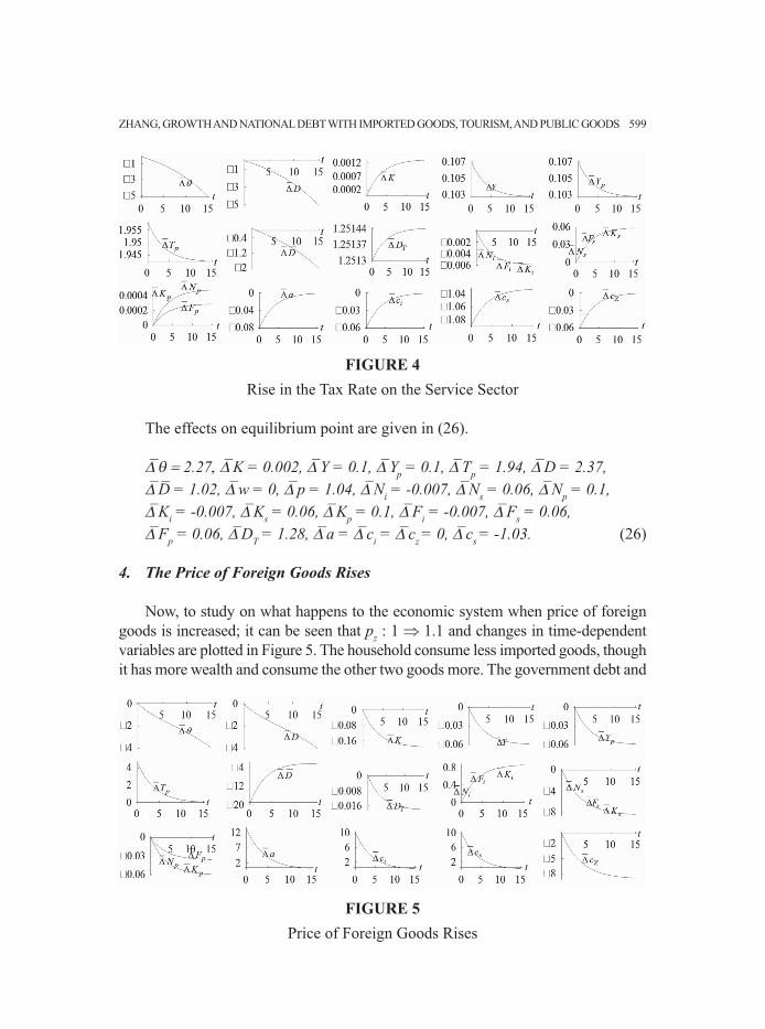
The effects on equilibrium point are given in (26).

– = 2.27, –K = 0.002, –Y = 0.1, –Yp = 0.1, –Tp = 1.94,

–D = 2.37,–D– = 1.02, –w = 0, –p = 1.04, –Ni = -0.007,

–Ns = 0.06, –Np = 0.1,

–Ki = -0.007, –Ks = 0.06,

–Kp = 0.1, –Fi = -0.007,

–Fs = 0.06,–Fp = 0.06,

–DT = 1.28, –a = –ci =

–cz = 0, –cs = -1.03. (26)

4. The Price of Foreign Goods Rises

Now, to study on what happens to the economic system when price of foreigngoods is increased; it can be seen that pz : 1 1.1 and changes in time-dependentvariables are plotted in Figure 5. The household consume less imported goods, thoughit has more wealth and consume the other two goods more. The government debt and


FIGURE 4Rise in the Tax Rate on the Service Sector

FIGURE 5Price of Foreign Goods Rises

national debt falls and the industrial sector expands; but the other two sectors shrinks.The economy uses less capital and produces less. The tax income rises and the na-tional expenditure on public goods falls. The result is that there are less tourists.


– = 0.03, –K = -0.19, –Y = -0.06, –Yp = -0.06, –Tp = -0.04,

–D = -0.03,–D– = -0.36, –w = 0, –p = 0, –Ni = 0.88,

–Ns = -8.7, –Np = -0.06,

–Ki = 0.88, –Ks = -8.7,

–Kp = -0.06, –Fi = 0.88,

–Fs = -8.7,–Fp = -0.04,

–DT = -0.02, –a = 0, –ci =0,

–cz = -9.09, –cs = 0. (27)

5. The Propensity to Save Rises

It can now be studied as to what happens to the economic system if price offoreign goods is increased, and 0 : 0.9 0.91. Changes in time-dependent vari-ables are plotted in Figure 6. The household has more wealth and consumes more,the industrial sector shrinks slightly but the other two sectors expands, the govern-ment debt and national debt falls. The economy uses less capital and produces more.The tax income rises and the national expenditure on public goods falls.


– = 0.2, –K = 0.004, –Y = 0.001, –Yp = 0.001, –Tp = 0.17,

–D = 0.2,–D– = -1.54, –w = 0, –p = 0, –Ni = -0.02,

–Ns = 0.2, –Np = 0.001,

–Ki = -0.02, –Ks = 0.2,

–Kp = 0.001, –Fi = -0.02,

–Fs = 0.2,–Fp = 0.001,

–DT = 0.0004, –a = 1.3, –ci = 0.2,

–cz = 0.2, –cs = 0.2. (28)


FIGURE 6Propensity to Save Rises

V. Conclusion

This paper develops an economic growth model of a small open economy withgovernment debt, tourism and imported goods in a perfectly competitive economy.The study focuses on effects of changes in preference; for imported goods, nationalexpenditure on supplying public goods and different taxes on the dynamic paths ofgovernment debt, trade balance and economic growth. The national economy consistsof three - industrial, service and public sectors. The assumption of small openeconomies implies that the rate of interest is fixed in the international market. Theproduction side is based on the neoclassical growth theory. The household behavioris modelled according to Zhang’s utility function. The nonlinear dynamic interactionis described between the economic structural change, capital accumulation and publicdebt, under different combinations of taxes on goods sector, the service sector, thewage income, rate of interest, consumption of goods, and the consumption of service.It simulates the model and demonstrate the system that has a unique unstable equi-librium point. The effect of changes in some parameters on behavior of the economicsystem is examined. The comparative dynamic analysis provides some important in-sights. It should be noted that the model is made with many strict assumptions whichmay extend and generalize it in different directions. For instance, it is important tostudy the economic dynamics when utility and production functions are taken onother functional forms. The government expenditure is a complicated issue. Howmuch to spend on different public goods may depend not only on the national income,but also on the other factors. The possibilities of domestic households travel othercountries are not considered. Monetary issues such as exchange rates and inflationpolicies are important for understanding the trade issues.

Bibliography

Andereck, K.L., K.M. Valentine, R.C. Knopf and C.A. Vogt, 2005, Residents’ percep-tions of community tourism impacts, Annals of Tourism Research, 32(4): 1056-76.

Antonakakis, N., M. Dragouni and G. Filis, 2015, How strong is the linkage betweentourism and economic growth in Europe? Economic Modelling, 44(January): 142-55.

Azariadis, C., 1993, Inter temporal macroeconomics, MA: Cambridge, Blackwell.Balaguer, L., and M. Cantavella-Jorda, 2002, Tourism as a long-run economic

growth factor: The Spanish Case, Applied Economics, 34: 877-84.Barro, R.J., 1990, Government spending in a simple model of endogenous growth,

Journal of Political Economy, 98: 103-25.


Barro, R., N.G. Mankiw and X. Sala-i-Martin, 1995, Capital mobility in neoclas-sical models of growth, American Economic Review, 85: 103-16.

Benigno, G. and P. Benigno, 2003, Price stability in open economies, Review ofEconomic Studies, 70: 743-64.

Blake, A., M.T. Sinclair and J.A. Campos, 2006, Tourism productivity - evidencefrom the United Kingdom, Annals of Tourism Research, 33: 1099-1120.

Blanchard, O.J., and S. Fischer, 1989, Lectures in macroeconomics, MA: Cam-bridge, MIT Press.

Burmeister, E., and A.R. Dobell, 1970, Mathematical theories of economic growth,London: Collier Macmillan Publishers.

Chalk, N., 2000, The sustainability of bond-financed deficits: An overlapping gen-erations approach, Journal of Monetary Economics, 45: 293-328.

Chao, C.C., B.R. Hazari, Y.P. Laffargue and E. S.HYu, 2009, A dynamic model oftourism, employment, and welfare: The Case of Hong Kong, Pacific EconomicReview, 14: 232-245.

Chou, M.C., 2013, Does tourism development promote economic growth intransition countries? A panel data analysis, Economic Modelling, 33(July):226-32.

Cohen, D., and J. Sachs, 1986, Growth and external debt under risk of debt repu-diation, European Economic Review, 30: 529-60.

Copeland, B.R., 1991, Tourism, welfare and de-industrialization in a small openeconomy, Economica, 58: 515-29.

Copeland, B.R., 2012, Tourism and welfare-enhancing export subsidies, The Japan-ese Economic Review, 63: 232-43.

Corden, W.M., and J.P. Neary, 1982, Booming sector and de-industrialization in asmall open economy, Economic Journal, 92: 825-48.

De la Croix, D., and P. Michel, 2002, A theory of economic growth, dynamics andpolicy in overlapping generations, Cambridge: Cambridge University Press.

Diamond, P., 1965, National debt in a neoclassical growth model, American Eco-nomic Review, 55: 1126-50.

Dritsakis, N., 2004, Tourism as a long-run economic growth factor: An empirical in-vestigation for Greece using causality analysis, Tourism Economics, 10: 305-16.

Drubarry, R., 2004, Tourism and economic growth: The case of Mauritius, TourismEconomics, 10: 389-401.

Dwyer, L., P. Forsyth and R. Spurr, 2004, Evaluating tourism’s economic effects:New and old approaches, Tourism Management, 25: 307-17.

Farmer, R., 1986, Deficits and cycles, Journal of Economic Theory, 40: 77–88.Gali, J., and T. Monacelli, 2005, Monetary policy and exchange rate volatility in a

small open economy, Review of Economic Studies, 72: 707-34. Gaŕin-Mũnos, T., 2007, German demand for tourism in Spain, Tourism Manage-

ment, 28: 12-22.


Giannitsarou, C., 2007, Balanced budget rules and aggregate instability: The roleof consumption taxes, Economic Journal, 117: 1423–35.

Gómez, M.A., 2008, Fiscal policy, congestion, and endogenous growth, Journal ofPublic Economic Theory, 10: 595-622.

Guo, J., and S. Harrison, 2004, Balanced-budget rules and macroeconomic (in) sta-bility, Journal of Economic Theory, 119: 357–63.

Hazari, B.R., and J.J. Lin, 2011, Tourism, terms of trade and welfare to the poor,Theoretical Economics Letters, 1: 28-32.

Hazari, B.R., and P.M. Sgro, 1995, Tourism and growth in a dynamic modelof trade, Journal of International Trade and Economic Development, 4:243-52.

Hazari, B.R., and P.M. Sgro, 2004, Tourism, trade and national welfare, Amsterdam:Elsevier.

Kim, H. J., M.H. Chen and S. Jang, 2006, Tourism expansion and economic devel-opment: The case of Taiwan, Tourism Management, 27: 925-33.

Kollmann, R., 2001, The exchange rate in a dynamic-optimizing business cyclemodel with nominal rigidities: A quantitative investigation, Journal of Interna-tional Economics, 55: 243-62.

Kollmann, R., 2002, Monetary policy rules in the open economy: Effects on welfareand business cycles, Journal of Monetary Economics, 49: 899-1015.

Kose, M.A., 2002, Explaining business cycles in small open economies: How muchdo world prices matter? Journal of International Economics, 56: 299-327.

Lane, P.R., 2001, The new open economy macroeconomics: A survey, Journal ofInternational Economics, 54: 235-66.

Lanza, A., P. Temple and G. Urga, 2003, The implications of tourism specialisationin the long run: An econometric analysis for 13 OECD Economies, TourismManagement, 24: 315-21.

Luzzi, G.F., and Y. Flückiger, 2003, Tourism and international trade: Introduction,Pacific Economic Review, 8: 239-43.

Marin-Pantelescu, A., and G. Tigu, 2010, Features of the travel and tourism industry whichmay affect pricing, Journal of Environmental Management and Tourism, 1: 8-11.

Matarrita-Cascante, D., 2010, Beyond growth: Reaching tourism-led development,Annals of Tourism Research, 32(4): 1141-63.

Matsuyama, K., 1987, Current account dynamics in a finite horizon model, Journalof International Economics, 23: 299-313.

Mendosa, E.G., 1995, The terms of trade, the real exchange rate, and economicfluctuations, International Economic Review, 36: 101-37.

Park, H., 2009, Ramsey fiscal policy and endogenous growth, Economic Theory,39: 377-98.

Obstfeld, M., and K. Rogoff, 1998, Foundations of international macroeconomics,MA: Cambridge, MIT Press.


Oh, C.O., 2005, The contribution of tourism development to economic growth inthe Korean economy, Tourism Management, 26: 39-44.

Sachs, J., 1982, The current account in the macroeconomic adjustment process,Scandinavian Journal of Economics, 84: 147-59.

Schubert, S.F., and J.G. Brida, 2009, A dynamic model of economic growth in asmall tourism driven economy, Munich Personal RePEc Archive.

Svensson, L.E.O., and A. Razin, 1983, The terms of trade and the current ac-count: The Harberger-Laursen-Metzler effect, Journal of Political Economy,91: 97-125.

Sinclair, M.T., and M. Stabler, 1997, The economics of tourism, London: Routledge. Semmler, W., and M. Sieveking, 2000, Critical debt and debt dynamics, Journal of

Economic Dynamics and Control, 24: 1121-44.Solow, R., 1956, A contribution to the theory of growth, Quarterly Journal of Eco-

nomics, 70: 65-94.Stabler, M.J., A. Papatheodorou and M.T. Sinclair, 2010, The economics of tourism,

London: Routledge. Syriopoulos, T.C., 1995, A dynamic model of demand for Mediterranean tourism,

International Review of Applied Economics, 9: 318-36.Turnovsky, S.J., 2000, Fiscal policy, elastic labor supply, and endogenous growth,

Journal of Monetary Economics, 45: 185-210.Turnovsky, S.J., 2004, The transitional dynamics of fiscal policy: Long-run capital

accumulation and growth, Journal of Money, Credit, and Banking, 36: 883-910.Turnovsky, S.J., and P. Chattopadhyay, 2003, Volatility and Growth in developing

economies: Some numerical results and empirical evidence, Journal of Inter-national Economics, 59: 267-95.

Turnovsky, B.J., and P. Sen, 1991, Fiscal policy, capital accumulation, and debt inan open economy, Oxford Economic Papers, 43: 1-24.

Uzawa, H., 1961, On a two-sector model of economic growth, Review of EconomicStudies, 29: 47-70.

Zeng, D.Z., and X.W. Zhu, 2011, Tourism and industrial agglomeration, The Japan-ese Economic Review, 62: 537-61.

Zhang, W.B., 1993, Woman’s labor participation and economic growth - creativity,Knowledge utilization and family preference, Economics Letters, 42: 105-10.

Zhang, W.B., 2005, Economic growth theory, London: Ashgate.Zhang, W.B., 2016, Public debt and economic growth in Uzawa’s two-sector model

with public goods, International Journal of Economic Sciences, 5(4): 52-73.Zhang, W.B., 2017, A small-open economic growth model with imported goods,

tourism, and terms of trade, Notas Económicas, July: 65-86.


APPENDIXProving the Lemma

From (2), the following equation is solved:

ki = ( -ii Ai )1/ i

, w = -i i Ai k ii. (A-1)

r

where, ki and w are considered as functions of r*.

s w wFrom (4), we obtain: ks = , p = . (A-2)s r -s

s As k ss

It is determined that ks and p are functions of r*, which implies that they aretime-independent, as shown in (20).From (8), we have,

p wkp = , (A-3) r

where, kp = Kp/Np

Now, we insert (A-1) – (A-3) in (9) to obtain,

ki N1 + ks Ns + kp Np = K. (A-4)

Equations (A-4) and (9) will follow to,

Ni + k1 Ns = k0 K - kn , (A-5)

1where, k0 , k1 (ks – kp) k0 , kn kp k0 N.ki – kp

Equations (11) and (12), will have,

y = -w w + (-a r* + 1) a. (A-6)

Inserting (A-6) in (14), we obtain


-w w + (-a r* + 1) a.cs = . (A-7)p

From Equations (1) and (3), the following equation is obtained,

Fi = Ai k ii Ni, Fs = As k s

s Ns (A-8)

Inserting (A-7) and (A-8) in (18), we obtain

-w Nw + (-a r* + 1) Na+ a- F

p p = As kss Ns (A-9)p

where (10) is used. From the definitions of ki and ks , we have

Ki = ki Ni , Ks = ks Ns (A-10)

From (6), we have, Yp = (Fi + pFs) (A-11)

Inserting (A-8) in (A-11), we have

Yp = Ai kii Ni + p As ks

s Ns. (A-12)

From (A-8) and (A-12), we have

Np = ai Ni + as Ns, (A-13)

p Ai k ii p p As ks

s where, ai , as . (A-14)w w

Insert kp = Kp/Np in (A-13)

Kp = kp ai Ni + Kp as Ns, (A-15)

Add (A-10) and (A-15),

K = (ki + kp ai) Ni + (ks + kp as) Ns, (A-16)

where, we use(9).


Insert (A-16) in (A-5) Ni = b0 - bNs , (A-17)

(ks + kp as) k0 - k1 knwhere, b , b0 (ki + kp ai) k0 - 1 (ki + kp ai) k0 - 1

Using (18), DT = Fs - cs N. (A-18)

It is noted that ki, ks, kp, w and p are determined as functions of r*. By the fol-lowing procedure we can determine all other variables as functions of Ns :a by (A-18) → Ni by (A-17) → K by (A-16) → Ki and Ks by (A-10) → Fi and Fs by (A-8)→ DT by (18) → y by (A-6) → c, cs, cz, s by (14) → Yp by (6) → Kp and Np by (8)→ Kp and Np by (8).

From (A9) and this procedure, we solve

(As kss Ns - a- F

p p ) p - -w Nwa = (Ns) (A-19)(-a r* + 1) N

From (15) and (17), we have

a. 0 (a) s - a, (A-20)

D.= D (D, Ns) r* D + Up - Tp (A-21)

Taking derivatives of (A-19) with respect to t

da. = N

.s (A-22)dNs

From (A-20) and (A-22), we have

( d )-1

N.s = N (Ns) 0 (A-23)dNs

Thus the lemma is proved.


growth and national debt with imported goods, tourism…

Documents