GROWTH AND DISTRIBUTIONAL DYNAMICS WITH LABOR MARKET AND INDUSTRIAL CONCENTRATION EFFECTS*

Michael Assous Department of Economics

University of Paris I, Pantheon-Sorbonne Paris

and

Amitava Krishna Dutt

Department of Political Science University of Notre Dame

Notre Dame, IN 46556

August, 2010

The interaction between economic growth and income distribution is examined using Kaleckian/post-Keynesian models in which there are lags in investment and in which the dynamics of income distribution between wages and profits depends on both labor market and industrial concentration effects. By examining these two influences on distributional dynamics simultaneously, the relative strength of which can change over the growth process, it is shown that the growth-distributional dynamics can involve non-linearities, multiple equilibria and instability. The implications of policy-induced changes – including those in macroeconomic policy and labor market and antitrust policies – on aggregate demand and distribution are examined for both wage-led and profit-led growth regimes.

Keywords: Income distribution, growth, Kaleckian/post-Keynesian models, aggregate demand

JEL Categories: E12, O41

* The work on this paper began when Dutt was visiting professor at the University of Paris 1, Pantheon-Sorbonne in March 2010.

0  

1. Introduction

What role do changes in labor market conditions and industrial concentration have in

determining the dynamics of growth and distribution in capitalist economies? This paper

examines this question using simple Kaleckian/post-Keynesian models of growth and

distribution.

The interaction between growth and distribution is, of course, a major topic of interest

within the Kaleckian/post-Keynesian (henceforth, KPK) tradition. A great deal of attention has

been given in this tradition to the effect of a change in the distribution of income between

workers and profit-recipients on the rate of capital accumulation and output growth, and to the

possibilities of wage-led and profit-led growth,1 that is, whether an increase in the profit share

reduces or increases the rate of growth of the economy. Some attention has also been given to

what determines the dynamics of income distribution, to complete the analysis of the interaction

between growth and distribution. 2 This side of the literature has focused on changes in income

distribution due to changes in labor market conditions, in which a tightening of the labor market

results in an increase in the wage share due to a strengthening of the bargaining power of

workers vis-à-vis firms,3 and to changes in industrial concentration.4

This paper follows the usual KPK tradition in which at a point in time the degree of

monopoly determines the distribution of income between workers and capitalists or profit

recipients and examining how distribution, through its affect on aggregate demand, influences

capital accumulation and growth. The model has the post-Keynesian feature, following the

writings of Kaldor (1940) and Steindl (1952), of making desired investment depend positively on

output and capacity utilization. It follows Kalecki (1971) in making the degree of monopoly

depend both on labor market conditions and changes in industry structure as measured by

1  

industrial concentration, and in allowing for lags between investment plans and actual

investment expenditures.

The paper’s contribution lies in examining how the combination of different influences

on distributional dynamics and changes in their relative importance over the growth process,

more specifically, those emanating from changes in the state of bargaining power between

workers and firms and in industrial concentration, can lead to novel and different patterns of the

interaction between growth and distribution in capitalist economies. In particular, it shows how

the dynamics of growth and distribution can involve nonlinearities and multiple equilibria, with

important implications for policy-induced changes in aggregate demand and income distribution.

The rest of this paper proceeds as follows. Section 2 describes the structure of the basic

model. Section 3 examines the short-run equilibrium and long-run dynamic properties of the

model and examines the effects of shifts in autonomous aggregate demand and profit share

dynamics. Section 4 examines a variant of the model which allows for profit-led growth.

Section 5 concludes.

2. Structure of the model

We assume a simple closed economy, without government fiscal activity, which produces one

good with two factors of production, homogenous labor and capital where capital is the produced

good. The economy has two classes, workers who receive wages and capitalists who receive the

residual income, as profits.

Workers are assumed to spend all their income on consumption, while capitalists are

assumed to save a fraction, s, of profits. This implies that saving, as a ratio of capital stock, is

given by the standard equation

2  

S/K = s π u, (1)

where S is real saving, K the stock of physical capital, π the share of profits in income and u =

Y/K is the rate of capacity utilization, with Y the level of real income and output.

Firms set their price as a markup on labor costs using fixed coefficients, constant returns

to scale technology, so that we have

P = (1+z)Wa0, (2)

where P is the price level, z is the markup, W is the money wage and ao is the labor required to

produce a unit of output, which is given, since we abstract from technological change. Firms

typically hold excess capacity, so that we assume that u<1/a1, where a1 is the technologically-

possible minimum capital-output ratio. Unemployed labor is available in the economy at a

money wage which is taken to be given, for simplicity.5 Firms are assumed to change their level

of production and capacity utilization due to changes in the demand for goods.

Firms have given investment plans at a point in time which, as a ratio of capital stock, we

denote with g, so that

I/K = g (3)

In other words, actual investment is predetermined from past plans. Their desired investment

plan, however, is assumed to depend positively on the rate of capacity utilization along the lines

discussed by Kaldor (1940) Steindl (1952): a higher level of capacity utilization makes firms

desire a higher level of investment. Assuming a simple linear relationship, we have desired

investment as a ratio of capital stock given by

gd = γ0 + γ1u, (4)

3  

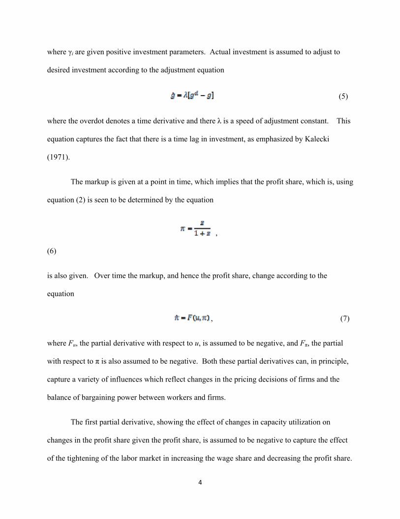
where γi are given positive investment parameters. Actual investment is assumed to adjust to

desired investment according to the adjustment equation

(5)

where the overdot denotes a time derivative and there λ is a speed of adjustment constant. This

equation captures the fact that there is a time lag in investment, as emphasized by Kalecki

(1971).

The markup is given at a point in time, which implies that the profit share, which is, using

equation (2) is seen to be determined by the equation

,

(6)

is also given. Over time the markup, and hence the profit share, change according to the

equation

, (7)

where Fu, the partial derivative with respect to u, is assumed to be negative, and Fπ, the partial

with respect to π is also assumed to be negative. Both these partial derivatives can, in principle,

capture a variety of influences which reflect changes in the pricing decisions of firms and the

balance of bargaining power between workers and firms.

The first partial derivative, showing the effect of changes in capacity utilization on

changes in the profit share given the profit share, is assumed to be negative to capture the effect

of the tightening of the labor market in increasing the wage share and decreasing the profit share.

4  

Instead of measuring labor market conditions in terms of the employment rate and assuming that

the supply of labor grows at some exogenous rate, which involves adding another state variable

to the system,6 we simplify and assume that the capacity utilization rate proxies the tightness of

the labor market. It is sometimes argued that an increase in capacity utilization, which reflects a

higher level of demand for goods, may induce firms to increase their markup at a higher rate, and

therefore increase the change in the profit share. However, such an effect is likely to be weak,

because with higher levels of demand firms may fear stronger threats of entry of new firms, and

this is likely to restrain, rather than strengthen, their tendency to raise the markup.7 Moreover, at

higher levels of capacity utilization the level of fixed costs per unit of output is lower, as Kalecki

(1971) argues, which is likely to reduce the need to increase markups to cover fixed costs, and

therefore reverse the tendency for the markup rate to increase more rapidly.

The second partial derivative, which shows the effect of a higher profit share on the

change in the profit share, given the level of capacity utilization, captures both the relative

bargaining power of workers and firm and industrial concentration effects. Regarding relative

bargaining power, Kalecki (1971, 161) wrote: “High markups in existence will encourage strong

trade unions to bargain for higher wages since they know that firms can ‘afford’ to pay them. If

their demands are granted but … [the markup is] not changed, prices also increase. This would

lead to a new round of demand for higher wages and the process would go on with price levels

rising. But surely an industry will not like such a process making its products more and more

expensive and thus less competitive with the products of other industries. To sum up, trade-union

power restrains the markups” We take this to mean that as the markup increases, firms will be

less able to pass on higher wage demands in the form of higher prices, so that the change in the

markup, and hence the profit share, will be lower. We assume that this effect is weak for lower

5  

levels of π, but becomes stronger at high levels of it when firms are strongly constrained by their

ability to pass on higher wage costs to higher prices. Regarding industrial concentration, we

assume that as the profit share falls, firms become more concerned about the fall in this share and

attempt to increase the rate of change of the markup by different means at their disposal,

including, through mergers and acquisition activity. Thus, as the profit share becomes smaller,

the rate of increase in the profit share falls. We assume that this effect is weak at higher levels of

π, but becomes stronger at lower levels of it since firms intensify their efforts to increase

markups when the markup becomes very low.

3. The dynamics of the economy

To analyze the dynamics of the economy we examine its behavior in two different runs. In the

short run we assume that K, g, and π are given, while in the long run these state variables are

allowed to change.

In the short run, firms adjust the level of output and hence, capacity utilization, according

to the demand for goods. For short-run equilibrium, therefore, we can determine the rate of

capacity utilization from the goods market clearing equation

Y = C + I

where C is the real level of consumption, which can be written as

I/K = S/K. (8)

Substituting from equations (1) and (3) we can solve for the equilibrium level of capacity

utilization,

6  

.

(9)

The equilibrium level of capacity utilization rises with g through the usual multiplier process,

falls with s due to the paradox of thrift, and falls with the profit share because of a shift in

income from workers who do not save to profit recipients who do. Aggregate demand is thus

wage led.

In the long run, abstracting from depreciation, for simplicity, we have

,

where overhats denote time-rates of growth. A change in K does not affect the short-run

equilibrium value of u. Also, g and π change according to the equations (5) and (7). Substituting

from equation (9), which always holds during the long run, and using equation (4) we obtain

, (10)

and

. (11)

The long-run dynamics of the simple two-dimensional system (there is no need to involve

K because it does not enter these equations) given by equations (10) and (11) can be analyzed

using a phase diagram in <g, π> space.

In Figure 1 the curve shows combinations of g and π for which g is stationary, and

is obtained by setting the right-hand side of equation (10) equal to zero, so that we have

7  

.

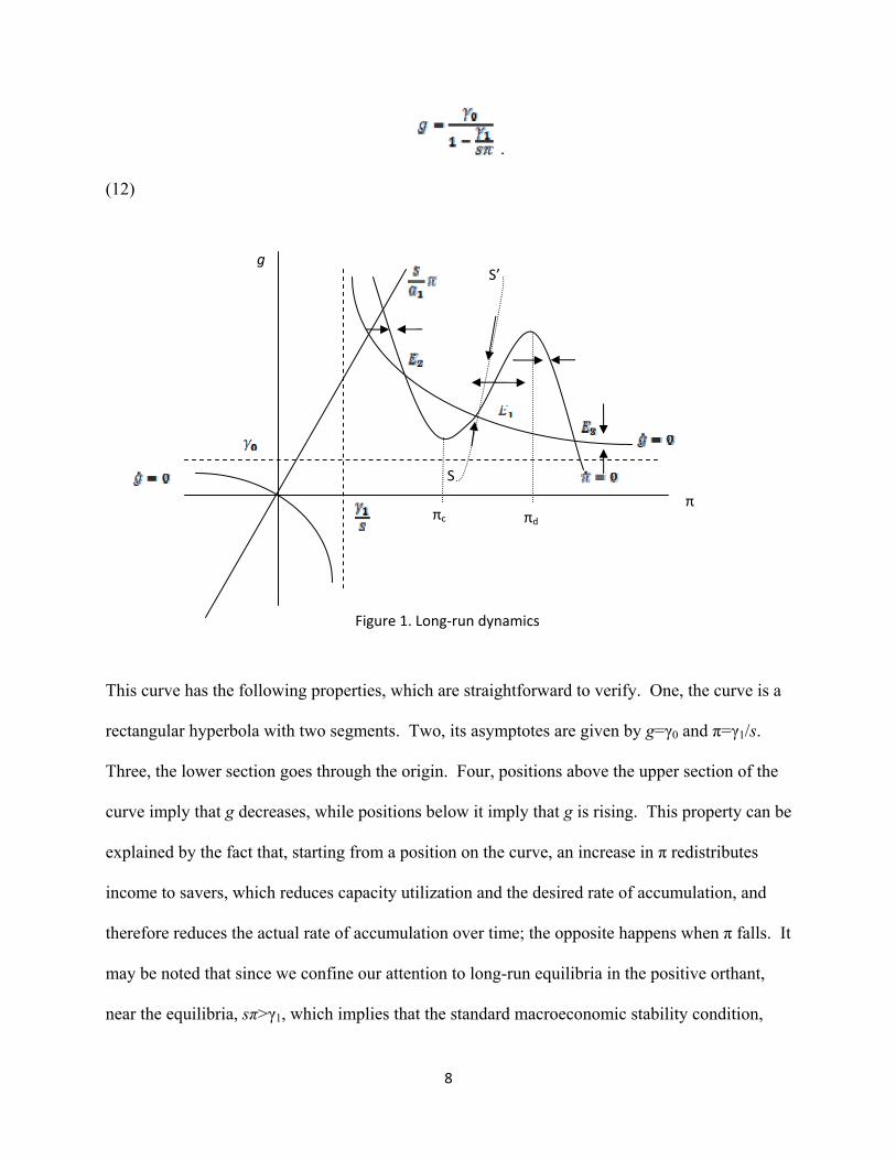
(12)

 

g 

π 

 

 

Figure 1. Long‐run dynamics 

 

S’ 

 

 

S 

πc  πd 

 

 

This curve has the following properties, which are straightforward to verify. One, the curve is a

rectangular hyperbola with two segments. Two, its asymptotes are given by g=γ0 and π=γ1/s.

Three, the lower section goes through the origin. Four, positions above the upper section of the

curve imply that g decreases, while positions below it imply that g is rising. This property can be

explained by the fact that, starting from a position on the curve, an increase in π redistributes

income to savers, which reduces capacity utilization and the desired rate of accumulation, and

therefore reduces the actual rate of accumulation over time; the opposite happens when π falls. It

may be noted that since we confine our attention to long-run equilibria in the positive orthant,

near the equilibria, sπ>γ1, which implies that the standard macroeconomic stability condition,

8  

according to which the responsiveness of saving to changes in capacity utilization exceeds that of

investment, is satisfied, ensuring that the dynamics of g, given π, is stable.

The curve shows combinations of g and π for which π is stationary. It is obtained

by setting the right hand side of equation (11) to zero. A rise in g necessarily reduces , since it

increases u by increasing aggregate demand, tightens the labor market, increases the wage share

and reduces the profit share. Thus, as shown in Figure 1, any point above (below) the curve

implies that π is falling (rising). The effect of a rise in π on is more complex, since there are

two separate effects which have to be taken into account. First, there is the direct effect of the

change in π on , which is a negative one because of both labor market and industrial

concentration effects. Second, there is the indirect effect which occurs due to changes in u: an

increase in π reduces u, which increases by tightening the labor market. This can be seen by

differentiating equation (11) with respect to π, which gives

where is the partial derivative of the function F with respect to i. Since and ,

the sign of this derivative is ambiguous. If we assume that the magnitude of the second term

does not change much in the relevant range examined by the model, while Fπ becomes larger in

absolute value when the profit share is very low (due to the industrial concentration effect) and

very high (due to the worker-firm bargaining effect), it follows that the derivative is likely to be

negative at particularly low and high levels of π (because of the dominance of the first term) but

positive (because of the dominance of the second term) for intermediate levels of π. If these

assumptions hold, then the slope of the locus, given by

9  

,

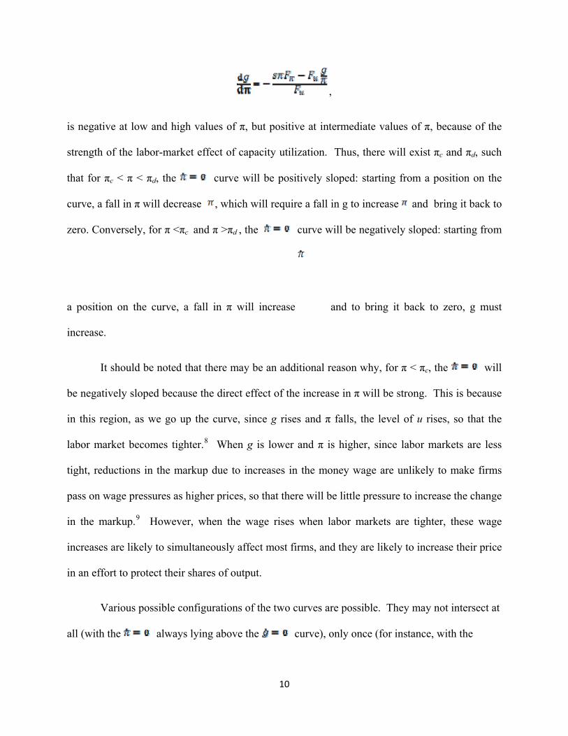
is negative at low and high values of π, but positive at intermediate values of π, because of the

strength of the labor-market effect of capacity utilization. Thus, there will exist πc and πd, such

that for πc < π < πd, the curve will be positively sloped: starting from a position on the

curve, a fall in π will decrease , which will require a fall in g to increase and bring it back to

zero. Conversely, for π <πc and π >πd , the curve will be negatively sloped: starting from

a position on the curve, a fall in π will increase and to bring it back to zero, g must

increase.

It should be noted that there may be an additional reason why, for π < πc, the will

be negatively sloped because the direct effect of the increase in π will be strong. This is because

in this region, as we go up the curve, since g rises and π falls, the level of u rises, so that the

labor market becomes tighter.8 When g is lower and π is higher, since labor markets are less

tight, reductions in the markup due to increases in the money wage are unlikely to make firms

pass on wage pressures as higher prices, so that there will be little pressure to increase the change

in the markup.9 However, when the wage rises when labor markets are tighter, these wage

increases are likely to simultaneously affect most firms, and they are likely to increase their price

in an effort to protect their shares of output.

Various possible configurations of the two curves are possible. They may not intersect at

all (with the always lying above the curve), only once (for instance, with the

10  

curve not sloping upwards enough to intersect the curve again at a low level of

π), twice (for instance, with the not sloping down sufficiently beyond πd to intersect the

curve again), or three times, as shown in Figure 1. The case of three intersections is

particularly interesting, and is worth discussing in some detail. It is obvious from the direction

of arrows in the figure that the equilibrium at E1, at a lower rate of growth and a higher profit

share, is saddlepoint-unstable. If the economy happens to start from a point on the separatrix

given by SS’, it will converge to the equilibrium at E1. But if it starts from a position to the right

(left) of this separatrix, the economy may eventually end up on a growth path in which it will

experience a fall (rise) in the rate of growth and a rise (fall) in the profit share till reaching

equilibrium E3 (E2). On such a path the dynamics can be understood from the fact that the

economy is wage led. When the profit share increases, the aggregate demand falls, capacity

utilization falls, the labor market loosens, the desired rate of accumulation falls, so that the profit

share rises further and the growth rate falls; the converse is true when the profit share falls,

which increases growth and results in further falls in the profit share as the labor market tightens.

This type of instability has been observed in standard post-Keynesian models with wage-led

growth which emphasize the effects of changes in labor market conditions on distribution. The

equilibriums at E2 and E3, at a higher rate of growth and a lower profit share, however, are both

stable equilibrium to which the economy will converge without cyclical fluctuations.

Two comments on these dynamics are in order. First, various possible trends of the

growth rate and the profit share may be observed on the long-run dynamic path of the economy.

For instance, if the economy is moving towards the long-run equilibrium at E2 from the regions

11  

between the two curves north-west or south-east of that equilibrium, an inverse relation between

movements in the growth rate and the profit share will be observed, and if the economy is

moving towards it from the south-west, it will experience an increase in the growth rate and a

rise in the profit share. Since cycles are possible, these relations between the rate of growth and

the profit share may also change over time. Thus, although we will refer to the model discussed

here, when we examine the effects of parametric changes, as exhibiting wage-led growth, we

cannot conclude that the wage share and the growth rate will always move in the same direction

in this model.

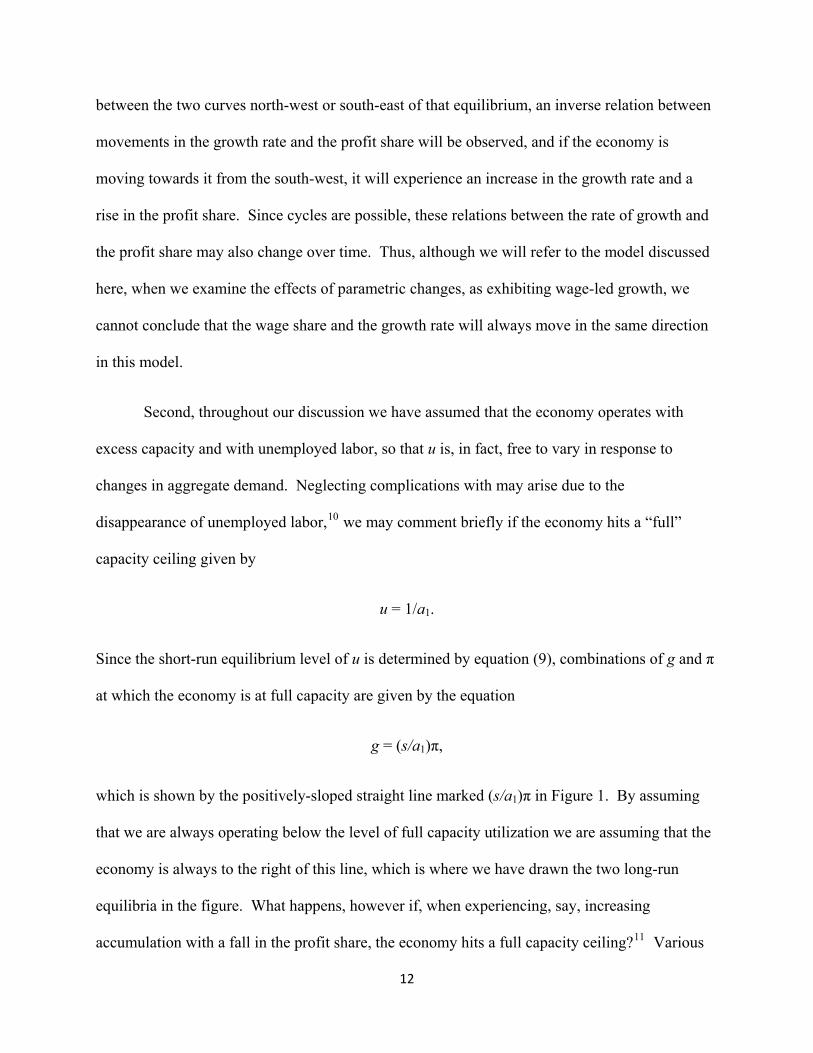
Second, throughout our discussion we have assumed that the economy operates with

excess capacity and with unemployed labor, so that u is, in fact, free to vary in response to

changes in aggregate demand. Neglecting complications with may arise due to the

disappearance of unemployed labor,10 we may comment briefly if the economy hits a “full”

capacity ceiling given by

u = 1/a1.

Since the short-run equilibrium level of u is determined by equation (9), combinations of g and π

at which the economy is at full capacity are given by the equation

g = (s/a1)π,

which is shown by the positively-sloped straight line marked (s/a1)π in Figure 1. By assuming

that we are always operating below the level of full capacity utilization we are assuming that the

economy is always to the right of this line, which is where we have drawn the two long-run

equilibria in the figure. What happens, however if, when experiencing, say, increasing

accumulation with a fall in the profit share, the economy hits a full capacity ceiling?11 Various

12  

outcomes are possible depending on what we assume about accumulation and profit share

adjustments when there is such a “regime” change. One possibility is that we continue to assume

that accumulation plans are always fulfilled, so that desired accumulation is given by gd =

γ0+γ1/a1, which is a constant, and actual accumulation evolves according to equation (5), but that

we jettison equation (6) and replace it with the assumption that π adjusts instantaneously to clear

the goods market. In other words, the economy will move along the full capacity locus,

experiencing a rise in g and a rise in π. This occurs because, owing to excess demand, for

instance, firms who are unable to increase capacity utilization any further, will increase their

price, increasing the markup. Thus, the long-run equilibrium will occur at the intersection of the

locus and the full capacity locus.12

To conclude this discussion of the long-run dynamics of the economy we consider the

cases in which the two curves, for and , intersect only once or do not intersect at

all. If they intersect only once, then there may be no stable equilibrium E2, so that the economy

be saddlepoint unstable. If it is on a wage-led growth path it will eventually hit full capacity

utilization, and the outcome can be analyzed as discussed in the previous paragraph. If the

locus lies everywhere above the locus, there will be no long-run equilibrium. In

this case the economy will (eventually) find itself on a dynamic path of declining accumulation

and worsening income distribution.

Having discussed these different possibilities, let us consider the effects of some

parametric shifts.

First, consider the effects of an exogenous increase in aggregate demand as represented

by an increase in the parameter γ0. In the short run, with g and π given, there will be no effect on

13  

the level of capacity utilization. However, the desired level of accumulation increases, and this

makes g increase. As can be checked from equation (12), the curve actually shifts up. In

we are in a situation with three equilibria, as is shown in Figure 1, the upward shift in this curve

will imply that if we start from the initial long-run equilibrium at E2, if the new stable long-run

equilibrium occurs at a position with excess capacity, the equilibrium growth rate will be higher

and the equilibrium profit share lower. Alternatively, if the economy hits the full capacity

barrier, it will experience a higher rate of accumulation, and the equilibrium profit share may go

up or down. If, instead, we start from the low equilibrium E3 on can see that a small upward shift

in the curve will increase g and reduce π in the long run, provided that the shift is less

than what is shown by the dotted line in Figure 2. But if there is a shift in the curve more than

what is shown by the dotted line, there will no longer be an equilibrium like E3, and the only

stable long-run equilibrium will be at the higher level. Thus, there will be a large increase in the

growth rate and a large rise in the wage share: the economy will move from a low-growth

equilibrium to a high-growth one.

If there is initially no long-run equilibrium because the curves do not intersect and the

economy was caught in a growth decline, the increase in autonomous demand can make the

curves intersect and stabilize the economy. If the economy is at a position to the right of the

separatrix, the increase in autonomous demand will shift the separatrix to the right, and possibly

move the economy from a path of declining growth to one of increasing growth.

14  

 

g 

π 

 

 

Figure 2. Effect of an autonomous increase in aggregate demand 

 S 

 

 

S’ 

   

It should also be noted that if we start from a high-growth equilibrium like E2, a fall in

autonomous aggregate demand of a large magnitude can move the economy to a low-growth

equilibrium like E3, with a dramatic fall in the growth rate and rise in the profit share, or even go

off in an unstable downward spiral (if there is no equilibrium like E3).

Second, consider the effect of an exogenous change in the determinants of , that,

changes other than those due to changes in u and π. Such a change could be due to changes in

government policies which, for instance, weaken the power of unions, and weaken anti-trust

legislation and implementation. For given levels of g and π, these changes have the effect of

increasing . Thus, a combination of g and π which was initially a point on the curve

will no longer be on it. To return to a point at which returns to zero we need to increase g,

which reduces by tightening the labor market. Thus, the curve shifts upwards.

15  

 

 

g 

 

 

 

S 

 

 

S’ 

 

π 

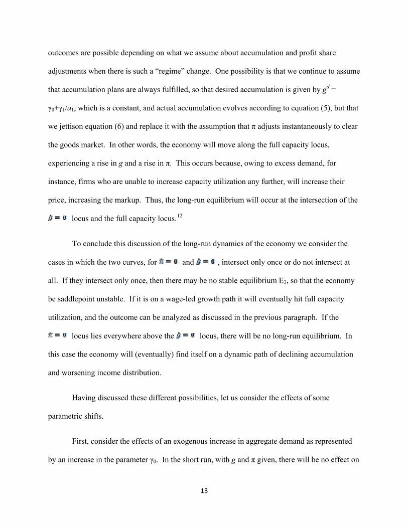
Figure 3. Effect of an autonomous change in income distribution towards profits 

Suppose we start at point E2. Since both g and π are given in the short run, there will be

no change in the rate of capacity utilization in the short run. As the curve shifts upwards,

for a given g, over time π will start increasing. If a high-growth equilibrium continues to exist,

that is, if the shifts less than what is shown by the dotted line in Figure 3, there will be a

long-run fall in g and a rise in π. But if the curve shifts up more than what is shown by the

dotted line, then there will no high-growth equilibrium, but only a low-growth one like the one

shown by E3. In that case the economy will move from a high-growth equilibrium to a low-

growth one with a dramatic increase in the profit share. Comparing the two situations just

described, it can be noted that in the first case a small increase in autonomous demand (through

fiscal expansion) can increase growth and increase the wage share, but in the second case, such a

policy-induced improvement in growth and distribution requires a much larger expansion in

16  

aggregate demand, and consequently is more difficult to achieve, given uncertainties in the

success of demand-induced expansions.

The effects of such changes are, in general, the opposite of what occurs when there is an

autonomous increase in demand. The stable long-run equilibrium will involve a lower growth

rate and a higher profit share, the possibility of no intersection is increased, and the separatrix

moves to the left, increasing the possibility of a growth decline.

Deregulation in the labor market (and a fall in the bargaining power of workers) is hence

likely to lead the economy to a low equilibrium characterized by high profit share and low

growth rate. Such changes, instead of eventually entailing more competition and growth as

authors such as Blanchard and Giavazzi (2003) assert is on, the contrary, likely to lead to more

concentrated markets competition and a low growth rate.

4. The case of profit-led growth

We have so far assumed that growth is wage led, that is, when the distribution of income goes

towards wages, consumption demand rises, and this causes capacity utilization to increase, which

increases investment demand and hence, the rate of growth of capital, the driving force behind

output growth. However, it is possible for growth to be profit-led instead, that is, a change in the

distribution of income ways from wages and towards profits, can increase the overall demand for

goods and the rate of growth of capital. While this can occur under a variety of circumstances, a

simple way of explaining this case is by amending the desired investment function by assuming

, (4’)

17  

with γ2 > 0, that is, by making desired investment depend positively on the profit share, in

addition to the rate of capacity utilization. This modification follows Bhaduri and Marglin

(1990), who assume that investment depends positively on the expected profit rate which, in

turn, depends positively on the profit share and the rate of capacity utilization, since the current

rate of profit, is given by r = πu. The rest of the model remains the same as before.

As before, the short-run equilibrium value of u is determined by equation (9). Using

equations (4/) and (5) we obtain the modified dynamic equation for g as

. (10’)

The relation between g and π which implies that is now given by

,

(12’)

which is shown by the in Figure 4. Confining our attention to the positive orthant we see

that the is a U-shaped curve, so that growth is wage-led at low levels of π and profit-led at

high levels of π. This follows from the assumed linearity of the desired investment function with

respect to both the rate of capacity utilization and the profit share. The is the same as

before, since it is given by equation (11), and its properties are the same as in the previous case.

18  

π 

g 

 

 

 

Figure 4. The case of profit‐led growth 

 

We consider in Figure 4 the case in which the two curves intersect only once, in the

positively-sloped section of the curve. In this case, there is only one long-run equilibrium

at the intersection of the two curves and it is stable. An exogenous increase in aggregate demand

shifts up the curve as before, and increases the growth rate and reduces the profit share,

as in the case of wage-led growth. However, an upward shift of the curve, say due to a

weakened bargaining position of workers, will increase π and g as well: an increase in the profit

share increases desired accumulation sufficiently to increase the rate of accumulation. Thus,

weakening the bargaining power of workers can promote growth, but if the goal is to improve

growth as well as distribution (that is, increase the wage share), it is better to do so by increasing

aggregate demand through expansionary demand policies rather than by weakening the position

of workers, say by weakening the power of labor unions.

19  

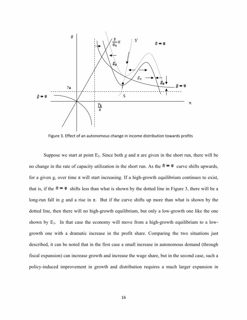
If the dynamics are as described in this case, it is not certain that there will be only one

long-run equilibrium. Figure 5 shows the dynamics with three equilibria. It can be checked that

the one at E1 is saddlepoint unstable, while those at E2 and E3 are stable. Although it is not

necessarily so, it is possible that the equilibrium at E2 is at the negatively-sloped portion of the

curve and that at E3 is at its positively-sloped portion. In this case, whether the economy

 π 

g 

 

 

 

E3 E2 

E1 

Figure 5. The case of multiple equilibria and the possibility of profit‐led 

starts from E2 or E3, an autonomous demand expansion, shifting the curve upwards will

increase growth and the wage share. But, an upward shift in the curve will reduce growth

and increase the profit share if the economy is at E2 (that is, the economy experiences profit-led

stagnation since the economy is in a wage-led growth regime) but increase growth and increase

the profit share if it as E3 (with the economy experiencing profit-led growth). A sufficiently

large upward movement in the may remove the equilibrium at E2, and make the rate of

20  

growth possibly increase as the distribution shifts towards profit at an equilibrium like E3.

However, there is no guarantee that equilibrium growth will actually increase (since it possible

for the initial equilibrium at E2 is at a higher rate of growth than the new equilibrium at a high-

profit share equilibrium qualitatively like E3, after the has moved up.

It should be noted that these possibilities arise because the curve is U-shaped, and

that this is so in our model because of the assumed linearity of the desired accumulation

function. If the function is not linear, and it is more likely that the economy is profit-led at low

levels of the profit share (as the economy is closer to full capacity utilization) than at high levels

of that share, then the curve will be inverse-U-shaped. In this case it is still true that if

there are three equilibria, there will be two stable equilibria, one at a high profit share and one at

a low profit share, and that, starting from either, an upward shift in the curve will

increase the growth rate and reduce the profit share. However, an upward shift in the will

now increase growth and increase the profit share at the low profit share equilibrium, but have

exactly the opposite effect in the high profit share equilibrium.

5. Conclusion

This paper has developed a simple Kaleckian-post-Keynesian model of growth and distribution

for which it has examined the short-run and long-run dynamics of the economy. Its main

contribution has been to allow for the existence of different reasons for distributional changes,

based on changes in the relative bargaining power of workers and firms, and changes in

industrial concentration, and for the possibility that the relative strength of these effects will

change depending on the its growth rate and the state of its income distribution. These

21  

considerations have allowed us to analyze the possibility of multiple equilibria and instability in

the dynamics of growth and distribution.

Assuming that desired investment depends positively on the level of capacity utilization

we have confirmed, as is well-known in the literature on Kaleckian-post-Keynesian models that

for the economy growth is wage led. But we have also shown that the economy may have high

and low growth stable equilibrium, at which expansionary macroeconomic policies will improve

both growth and distribution performance of the economy, and efforts to weaken labor and

introduce greater labor market flexibility negatively affects both growth and distribution. In fact

changes bringing about the latter can lead to dramatically poor growth performance, which

macroeconomic policies may find it very difficult to reverse.

We have also shown that if we allow for the possibility of profit-led growth,

expansionary macroeconomic policy continues to have positive growth and distributional effects,

and greater labor market flexibility and the weakening of labor’s bargaining power may or may

not increase growth (and the conditions for growth improvement through such policies cannot be

predicted simply on the basis of whether the profit share is initially high or low), and if it does, it

may do so only by worsening income distribution.

Our analysis also implies that if growth is wage led, the growth path may be self limiting,

but not necessarily self-defeating. It could be argued that increases in the wage share will lead to

a backlash due to changes in the behavior of firms and capitalists and consequent changes in

industrial concentration. This model shows that if this backlash does occur due to endogenous

changes in the profit share, the positive effects on income distribution due to increases in the

wage share, and the positive effects of this on the rate of growth of the economy, may be halted

22  

by such a backlash. However, the gains are likely to be permanent, in the sense that the backlash

will not reverse the wage and growth gains. However, if the backlash takes the form of an

exogenous (at least in terms of our model) political backlash, involving an autonomous change in

distributional dynamics, growth and distributional reversals become possible. But it is important

to keep in mind the distinction between endogenous economic changes due to changes in the

behavior of firms and capitalists and backlashes which involve more ideological and political

changes. The former may well occur, but there is nothing inevitable about the latter. This is

fortunate, because without it, the economy’s growth and distributional prospects are rosier.

We should end by noting that our analysis has been conducted with the use of a simple

theoretical model of growth and distribution which has abstracted from many important features

of real economies. Two such features involve financial and open-economy considerations, which

have been entirely neglected from our analysis, both of which have received a fair amount of

attention in Kaleckian-post-Keynesian modeling. It would be of some interest to integrate the

implications of our analysis with those of the models in this literature. There has also been some

effort at the empirical investigation of the relation between growth and distribution, that is, in

examining whether in actual economies growth is growth is wage led or profit led. While this

analysis can provide input in deciding when, for instance, labor market reforms may have more

negative consequences, our analysis also has some implications for the difficulties of deciding on

this issue using empirical data because of the possible non-monotonicity of the distribution

curve showing distributional change, and the difficulties of distinguishing between changes in

the curves and movements along dynamic paths given the parameters of the model.13

23  

REFERENCES

Bhaduri, Amit and Marglin, Stephen A. (1990). “Unemployment and the real wage: the economic basis of contesting political ideologies”, Cambridge Journal of Economics, 14(4), 375-93.

Blanchard, Olivier and Giavazzi, Francesco (2003). “Macroeconomic Effects of Regulation And Deregulation In Goods And Labor Markets”, Quarterly Journal of Economics, 118(3), 879-907.

Dutt, Amitava Krishna (1984). “Stagnation, income distribution and monopoly power”, Cambridge Journal of Economics, 8(1), 25-40.

Dutt, Amitava Krishna (1990). Growth, distribution and uneven development, Cambridge, UK: Cambridge University Press.

Dutt, Amitava Krishna (1992). “Conflict inflation, distribution, cyclical accumulation and crisis”, European Journal of Political Economy, 8(1), 579-97.

Dutt, Amitava Krishna (2006). “Aggregate demand, aggregate supply and economic growth”, International Review of Applied Economics, 20(3), 319-336.

Dutt, Amitava Krishna (2010). “Distributional dynamics in post-Keynesian growth models”, paper presented at the conference on Recent Developments in Post-Keynesian modeling, University of Paris 13, November, 2009, forthcoming, Journal of Post Keynesian Economics.

Goodwin, R. M. (1967). “A Growth Cycle”, in C. H. Feinstein, ed., Socialism, Capitalism and Growth, Cambridge University Press, Cambridge.

Henley, A. (1987).  “Trades unions, market concentration and income distribution in United States manufacturing industry”, International Journal of Industrial Organization, 5(2), 193-210.

Kaldor, Nicholas (1940). “A model of the trade cycle”, Economic Journal, 50, 78-92.

Kalecki, Michal (1943). Studies in economic dynamics, London: George Allen and Unwin.

Kalecki, Michal (1971). Selected essays on the dynamics of the capitalist economy, Cambridge, UK: Cambridge University Press.

Lima, Gilberto Tadeu (2000). “Market concentration and technological innovation in a dynamic model of growth and distribution”, Banca Nazionale del Lavoro Quarterly Review, 215, 447–75.

Nikiforis, Michalis and Foley, Duncan (2010). “Empirical evidence on the relation between distribution and capacity utilization”, unpublished, Department of Economics, New School University. Rowthorn, Robert (1982). “Demand, real wages and growth”, Studi Economici, 18, 3-54.

24  

Steindl, Josef (1952). Maturity and Stagnation in American Capitalism, Oxford: Blackwell.

Taylor, Lance (1991). Income Distribution, Inflation and Growth, Cambridge, Mass.: MIT Press.

Taylor, Lance (2004), Reconstructing Macroeconomics, Cambridge, Mass.: Harvard University Press.

25  

26  

                                                           

NOTES

 1 See, for instance, Rowthorn (1981), Dutt (1984, 1990), Bhaduri and Marglin (1990) and Taylor (1991, 2004).  2 See Dutt (2010) for a discussion of different approaches and their incorporation into post-Keynesian growth models.  3 See, for instance, Taylor (1991, 2004) and Dutt (1992).  4 See Dutt (1984) and Lima (2000).  5 Nothing is changed if money wages are assumed to change. Given the markup and the labor-output ratio it will just result in a proportionate increase in the price level, and result in price inflation. Of course, inflation can result in changes in the distribution of income due to changes in the markup, as discussed, for instance, in Dutt (1990, 1992) and Taylor (1991) but these issues are not analyzed in this paper.  6 This specification is pursued in Dutt (1992).  7 To the extent that higher levels of demand induce greater entry, there may also be a tendency for the degree of industrial concentration to fall, thereby reducing the tendency of the markup and the profjt share to increase.  8 As equation (9) shows, the level of capacity utilization is constant along a positively-sloped ray through the origin, and is higher as this line rotates upwards.  9 In fact, if firms are profit maximizers and face a kinked demand curve, they may not change the price at all when the wage rises (see Henley, 1987).  10 Labor supply growth may be endogenous. Moreover, endogenous labor productivity growth of the form analyzed in Dutt (2006) is also likely to prevent the depletion of unemployed labor.  11 This occurs when E2 lies to the left of the (s/a1)π locus.  12 Alternative outcomes are possible if it is assumed that if desired investment exceeds actual investment, firms are unable to increase their rate of investment, so that g becomes stationary at full capacity, and the dynamics of π continue to be given by equation (7), or if there is partial immediate adjustment of both changes in g and π. The implications of these possibilities are not explored here because they are not central to the concerns of this paper.  13 In the course of writing this paper we have become aware of an interesting empirical paper by Nikiforos and Foley (2010) which provides some evidence, although weak, that the distributive schedule – which is related to the curve showing stationary levels of the profit share – is not monotonic.