growth accounting for the euro area: a structural approach · growth accounting for the eur o area...

ISSN 1561081-0

9 7 7 1 5 6 1 0 8 1 0 0 5

WORKING PAPER SER IESNO 804 / AUGUST 2007

GROWTH ACCOUNTING FOR THE EURO AREA

A STRUCTURAL APPROACH

by Tommaso Proiettiand Alberto Musso

In 2007 all ECB publications

feature a motif taken from the €20 banknote.

WORK ING PAPER SER IE SNO 804 / AUGUST 2007

Workshop “Perspectives on Potential Output and Productivity Growth” (Enghien-Les-Bain, Paris, 24-25 April 2006) organised by the Banque de France and the Bank of Canada. Section 4.3 is based on a suggestion by Gonzalo Camba-Mendez. The views

expressed in this paper do not necessarily reflect those of the European Central Bank.2 S.E.F. e ME. Q, University of Rome, Tor Vergata, Via Columbia 2, 00133 Rome, Italy; e-mail: [email protected]

3 Address for correspondence: Directorate General Economics, European Central Bank, Kaiserstrasse 29, 60311 Frankfurt am Main, Germany; e-mail: [email protected]

This paper can be downloaded without charge from http://www.ecb.int or from the Social Science Research Network

electronic library at http://ssrn.com/abstract_id=1006995.

GROWTH ACCOUNTING FOR THE EURO AREA

A STRUCTURAL APPROACH 1

by Tommaso Proietti 2

and Alberto Musso 3

1 We would like to thank several people for useful discussions and valuable comments, including Gonzalo Camba-Mendez, Marc-Andre Gosselin, Neale Kennedy, Geoff Kenny, Hans-Joachim Klöckers, Gerard Korteweg and participants to an ECB seminar and the

© European Central Bank, 2007

AddressKaiserstrasse 2960311 Frankfurt am Main, Germany

Postal addressPostfach 16 03 1960066 Frankfurt am Main, Germany

Telephone +49 69 1344 0

Internethttp://www.ecb.europa.eu

Fax +49 69 1344 6000

Telex411 144 ecb d

All rights reserved.

Any reproduction, publication and reprint in the form of a different publication, whether printed or produced electronically, in whole or in part, is permitted only with the explicit written authorisation of the ECB or the author(s).

The views expressed in this paper do not necessarily reflect those of the European Central Bank.

The statement of purpose for the ECB Working Paper Series is available from the ECB website, http://www.ecb.europa.eu/pub/scientific/wps/date/html/index.en.html

ISSN 1561-0810 (print)ISSN 1725-2806 (online)

3ECB

Working Paper Series No 804August 2007

CONTENTS

Abstract 4

Non-technical summary 5

1 Introduction 72 The model 9 2.1 The production function compositional approach 9 2.2 The Multivariate Model 11

3 The empirical analysis 15 3.1 Database description 15 3.2 Estimation results 16

4 The procyclicality of potential ouput estimates 19 4.1 Issues related to the procyclicality of potential ouput estimates 19 4.2 A model-based low-pass filtering of potential output 20 4.3 Does the procyclicality of potential output matter? 25

5 Stylised facts of potential output growth in the euro area based on the structural growth accounting approach 27

6 Conclusions 30

References 32

Appendix A - Approaches to deal with the procyclicality of potential ouput estimates 35

Tables and figures 37

European Central Bank Working Paper Series 44

Abstract

This paper is concerned with the estimation of euro area potential output growth and its decomposition

according to the sources of growth. The growth accounting exercise is based on a multivariate struc-

tural time series model which combines the decomposition of total output according to the production

function approach with price and wage equations that embody Phillips type relationships linking in-

flation and nominal wage dynamics to the output gap and cyclical unemployment, respectively.

Assuming a Cobb-Douglas technology with constant returns to scale, potential output results from

the combination of the trend levels of total factor productivity and factor inputs, capital and labour

(hours worked), which is decomposed into labour intensity (average hours worked), the employment

rate, the participation rate, and population of working age. The nominal variables (prices and wages)

play an essential role in defining the trend levels of the components of potential output, as the latter

should pose no inflationary pressures on prices and wages.

The structural model is further extended to allow for the estimation of potential output growth

and the decomposition according to the sources of growth at different horizons (long-run, medium

run and short run); in particular, we propose and evaluate a model–based approach to the extraction

of the low–pass component of potential output growth at different cutoff frequencies. The approach

the boundaries of the sample period, so that the real time estimates do not suffer from what is often

referred to as the ”end–of–sample bias”. Secondly, it is possible to assess the uncertainty of potential

output growth estimates with different degrees of smoothness.

4ECB Working Paper Series No 804August 2007

has two important advantages: the signal extraction filters have an automatic adaptation property at

Keywords: Potential output, Output gap, Euro area, Unobserved components, Production function approach, Low-pass filters. JEL classification: C32, C51, E32, O47

Non-technical summary

The main purpose of this paper is to propose an extended empirical approach to estimate and analyse

potential output growth and to apply it to the case of the euro area. This contribution can be also

seen as proposing a structural approach to growth accounting. The reference framework adopted is a

model based approach: we specify and estimate a multivariate structural time series model embodying

the decomposition of output according to a production function approach and two Phillips type rela-

tionships relating price and wage inflation to the output gap and the unemployment gap, respectively.

Assuming a Cobb-Douglas technology with constant returns to scale, potential output results from the

combination of the trend levels of total factor productivity and factor inputs, capital and labour (hours

worked), which is decomposed into labour intensity (average hours worked), the employment rate,

the participation rate, and population of working age. The nominal variables (prices and wages) play

an essential role in defining the trend levels of the components of potential output, as the latter should

pose no inflationary pressures on prices and wages. Typically, estimates of potential output growth

based on this framework, as well as on simpler approaches, tend to exhibit a marked procycical pat-

tern, unless some smoothness prior is imposed. As shown in the application, this is the case also for

the euro area. Against this background, one of the key contributions of the paper is to propose an ex-

tension of the basic statistical framework allowing for a formal analysis of the degree of smoothness

of the growth rate of potential output and its components. More precisely, we propose a model-based

filtering approach for estimating potential output growth at different horizons, namely in the medium

and long run. For this purpose the band-pass decomposition of potential output is embedded within

the original parametric model so that we are able to estimate the underlying growth at any relevant

horizon also in real time and to assess its reliability using standard optimal signal extraction princi-

ples. Finally, we provide a novel way of estimating the level of smoothness that is consistent with

the definition of potential output and the NAIRU as those components of output and unemployment

that exerts no inflationary pressure on prices and wages. The approach we propose has two important

advantages. First, the signal extraction filters have an automatic adaptation property at the boundaries

of the sample period, so that the real time estimates do not suffer from what is often referred to as the

5ECB


”end-of-sample bias”. Second, it allows for an assessment of the uncertainty surrounding potential

output growth estimates with different degrees of smoothness. The application focuses on the case

of the euro area. Using our extended framework, we provide a discussion of potential output growth

developments and its main sources since 1970. Moreover, we illustrate to which extent the reliability

of potential output growth estimates for the euro area decreases as the imposed degree of smoothness

increases. A finding of the applied exercise is that the estimates of potential output resulting from our

original model do not carry additional information that is relevant for explaining the behaviour of the

nominal variables, although they have a procyclical appearance. Overall, the application makes clear

that the proposed extended framework allows for a formal analysis of various key aspects of poten-

tial growth, thereby representing a potentially important methodological contribution in the empirical

analysis of growth and its sources.


1 Introduction

The notion of potential output, defined by Okun (1962) as the maximum level of output the economy

can produce without inflationary pressures, plays an important role in macroeconomic analysis. In

the European context, estimates of potential output and the deviations of actual output from potential,

known as the output gap, provide relevant information for the conduct of economic policy. From a

monetary policy perspective, these estimates are one of the factors from which a reference value for

measures of structural budget deficits, which play a key role in the context of the Stability and Growth

Pact. Moreover, from a structural policy perspective, they can provide indications on the sustainability

of growth developments as well as on the need for further reforms in the labour and product market,

also against the background of the targets of the Lisbon strategy.

The main purpose of this paper is to estimate and analyse potential output developments in the euro

area during the period 1970-2005. We perform a growth accounting analysis that emerges directly

from fitting a multivariate structural time series model which combines the decomposition of total

output obtained by the production function approach with two price and wage equations that embody a

Phillips type relationship relating inflation and nominal wage dynamics to the output gap and cyclical

unemployment, respectively.

The structural model extends that entertained by Proietti, Musso and Westermann (2007) (hence-

forth referred to as PMW) in two directions: first, the measure of labour input that is adopted is hours

worked rather that the number of employed persons. This enriches the framework of the analysis,

allowing for a breakdown of this production factor into four components: labour intensity (average

hours worked), the employment rate, the participation rate, and a demographic factor, concerning

the evolution of the working age population. This choice is also more in line with the traditional

production function analysis, and bears important consequences on the estimation of total factor pro-

ductivity growth. Secondly, an additional equation is specified relating nominal wages to the deviation

of unemployment from structural unemployment, or NAIRU (non-accelerating inflation rate of unem-

ployment, i.e. the rate of unemployment that is consistent with a stable rate of inflation), or, as it is

7ECB


monetary growth is derived (see ECB, 2004). As for fiscal policy, they are instrumental for deriving

sometimes called, the NAWRU (non-accelerating wage inflation rate of unemployment). As a result,

we base our analysis on a multivariate structural time series model that is formulated in terms of seven

variables, namely, total factor productivity, average hours worked, the participation rate, the contribu-

tion of the unemployment rate, a capacity utilisation measure, the consumer price index, and nominal

wages.

Assuming a Cobb-Douglas technology with constant returns to scale, potential output results from

the combination of the trend levels of total factor productivity and factor inputs, labour and capital.

The nominal variables (prices and wages) play an essential role in defining the trend levels of the

above mentioned variables, as they should pose no inflationary pressures on prices and wages.

The structural model is further extended to allow for the estimation of potential output growth and

its decomposition into sources at different horizons (long-run, medium run and short run); in particu-

lar, we propose and evaluate a model–based approach to the extraction of the low–pass component of

potential output growth at different cutoff frequencies. The approach has two important advantages:

the signal extraction filters have an automatic adaptation property at the boundaries of the sample

period, so that the real time estimates do not suffer from what is often referred to as the ”end–of–

sample bias”. Secondly, it is possible to assess the uncertainty of potential output growth estimates

with different degrees of smoothness.

Discussions of the appropriate or desirable degree of smoothness of potential output estimates

most often are undertaken in an informal way, e.g. by setting to an ad hoc value a particular parameter

which regulates the smoothness. Several studies, for example with reference to the NAIRU, follow

the approach of Gordon (1998) and apply a smoothness prior without a formal analysis to justify it.

In this paper we show how it is possible to extend the statistical framework adopted to allow for a

formal discussion of the degree of smoothness of potential output and its components.

The paper is structured as follows. Section 2 summarises the production function approach and

illustrates the specification of the structural model. Section 3 reports and discusses in detail the

estimation results. Section 4 discusses the estimation of potential output growth at different time

horizons by model–based low–pass filtering. Section 5 elaborates on the growth accounting analysis


allowed for by the structural approach we propose. Finally, section 6 summarises the conclusions that

can be drawn from the analysis.

2 The model

This section describes the multivariate structural time series model upon which our growth accounting

analysis is based. We begin by reviewing the method of decomposing output fluctuations known as

the production function approach.

2.1 The production function compositional approach

The production function approach (PFA) is a multivariate method that obtains potential output from

the ”non-inflationary” levels of its structural determinants, such as productivity and factor inputs.

Let yt denote the logarithms of output (gross domestic product), and consider its decomposition

into two components,

yt = µt + ψt,

where µt, potential output, is the expression of the long run behaviour of the series and ψt, denoting

the output gap, is a stationary component, usually displaying cyclical features. Potential output is

the level of output consistent with stable inflation, whereas the the output gap is an indicator of

inflationary pressure.

We assume that the technology can be represented by a Cobb- Douglas production function with

constant return to scale on labour and capital:

yt = ft + αht + (1− α)kt. (1)

where ft is the Solow residual, ht is hours worked, kt is the capital stock (all variables expressed in

logarithms), and α is the elasticity of output with respect to labour (0 < α < 1).

To achieve the decomposition yt = µt + ψt, the variables on the right hand side of equation (1) are

broken down additively into their permanent (denoted by the superscript P ) and transitory (denoted

9ECB


by the superscript T ) components, giving:

ft = f (P )

t + f (T )

t , ht = h(P )

t + h(T )

t , kt = k(P )

t . (2)

It should be noticed that potential capital is always assumed to be equal to its actual value; this is so

since capacity utilisation is absorbed in the cyclical component of the Solow’s residual. Only survey

based measures of capacity utilisation for the manufacturing sector are available for the euro area.

Hence, potential output is the value corresponding to the permanent values of factor inputs and the

Solow residual, while the output gap is a linear combination of the transitory components:

µt = f (P )

t + αh(P )

t + (1− α)kt,

ψt = f (T )

t + αh(T )

t .(3)

Under perfect competition the output elasticity of labour, α, can be estimated from the labour share

of output. For the euro area the average labour share obtained from the national accounts (adjusted

for the number of self-employed) is about 0.65.1

Hours worked can be separated into four components that are affected differently by the business

cycle, as can be seen from the identity ht = nt + prt + ert +hlt, where nt is the logarithm of working

age population (i.e., population of age 15-64), prt is the logarithm of the labour force participation rate

(defined as the ratio of the labour force over the working age population), ert is that of the employment

rate (defined here as the ratio of employment over the labour force), and hlt is the logarithm of labour

intensity (i.e., average hours worked). Each of these determinants is in turn decomposed into its

permanent and transitory component in order to obtain the decomposition:

h(P )

t = nt + pr(P )

t + er(P )

t + hl(P )

t , h(T )

t = pr(T )

t + er(T )

t + hl(T )

t . (4)

The idea is that population dynamics are fully permanent, whereas labour force participation, em-

ployment and average hours are also cyclical. Moreover, since the employment rate can be restated in1Although the choice of a Cobb-Douglas production function with constant factor income shares is to some extent

controversial and the evidence for the euro area in this respect is scarce, Willman (2002) provides some evidence in

favour of such a production function for the euro area. See Musso and Westermann (2005) for adjusted estimates of the

euro area labour share. The greatest advantage of the Cobb-Douglas specification is its additivity on the logarithmic scale.


terms of the unemployment rate, we can relate the output gap to cyclical unemployment and poten-

tial output to structural unemployment. As a matter of fact, the unemployment rate being one minus

the employment rate, the variable curt = −ert (the contribution of the unemployment rate, using a

terminology due to Runstler, 2002), is the first order Taylor approximation to the unemployment rate.

Thus, cur(P )

t can be assimilated to the NAIRU and cur(T )

t to the unemployment gap.

As it is well known, there are several alternative ways of obtaining the trend components of the

individual determinants; our approach will provide a parametric dynamic representation for the com-

ponents and will relate them to nominal variables, prices and wages, so as to enforce the definition of

potential output as the level that is consistent with stable inflation. The introduction of the nominal

variables is essential for discriminating the permanent (supply) from the transitory (demand) varia-

tions. In our application we shall consider both the consumer price index and nominal wages, and

relate their variation to the output and the unemployment gap, respectively.

2.2 The Multivariate Model

The multivariate unobserved components model for the estimation of potential output and the output

gap, implementing the PFA outlined in the previous sub-section, is formulated in terms of the seven

variables already mentioned

[ft, hlt, prt, curt, ct, pt, wt]′ = [y′t, pt, wt]

′.

The variable ct is the logarithm of capacity utilisation. The variables are divided into two blocks. The

first block defines the permanent-transitory decomposition of yt = [ft, hlt, prt, curt, ct]′, and

yields potential output and the output gap according to the PFA. The second block is constituted by

the price and wage equations, which relate underlying inflation to the output gap and nominal wages

dynamics to the unemployment gap.

For yt, we specify the following system of time series equations:

yt = µt + ψt + ΓXt, t = 1, . . . , T, (5)

11ECB


where µt = {µit, i = 1, . . . , 5} is the 5× 1 vector containing the permanent levels of ft, hlt,prt, curt,

and ct, ψt = {ψit, i = 1, . . . , 5} denotes the transitory component in the same series, and ΓXt are

fixed effects.

The permanent component is specified as a multivariate integrated random walk:

∆2µt = ζt, ζt ∼ NID(0,Σζ). (6)

Here ∆ = 1 − L denotes the difference operator, and L is the lag operator, such that Lyt = yt−1;

NID stands for normally and independently distributed. It is assumed that the disturbance covariance

matrix has rank 4. This restriction enforces the stationarity of ct around a deterministic trend, possibly

with a slope change, and amounts to zeroing out the elements of Σζ referring to ct, and introducing a

slope change variable in Xt. For more details about the trend in capacity see PMW.

The matrix Xt contains interventions that account for a level shift both in prt and curt in 1992.4,

an additive outlier (1984.4) and a slope change in 1975.1 in capacity utilisation, ct; Γ is the matrix

containing their effects.

The specification of second-order trends postulates that the underlying growth changes slowly over

time if the size of Σζ is small compared to the variance of the cyclical components. PMW discuss

some of the most relevant specification issues that arise with respect to the characterisation of the

trend components in the variables under analysis and the isolation of the transitory component of

unemployment rates and labour participation rates. The various specifications are compared in PMW

on the grounds of their data coherency, predictive validity and the reliability of the corresponding

output gap.

With respect to the cyclical components, ψit, i = 1, . . . , 5, among the various alternative specifica-

tions considered by PMW, in this paper we adopt the pseudo-integrated cycles model. The key aspect

of this specification is that it is assumed that the cyclical component of each variable is driven by both

the economy-wide business cycle and an idiosyncratic cycle. In particular, we take the cycle in ca-

pacity as the reference cycle, writing ψ5t = ψt, where ψt is the stationary second order autoregressive

process

ψt = φ1ψt−1 + φ2ψt−2 + κt, κt ∼ NID(0, σ2κ). (7)


The roots of the autoregressive polynomial are a pair of complex conjugates. This restriction

is enforced by the following reparameterisation: φ1 = 2ρ cos λc, φ2 = −ρ2, with ρ ∈ (0, 1) and

λc ∈ [0, π]. For the cycle in the i-th variable (i = 1, 2, 3, 4) , where i indexes ft, hlt, prt, curt,

ψit = ρiψi,t−1 + θi(L)ψt + κit, κit ∼ NID(0, σ2κ,i) (8)

where κit is an idiosyncratic disturbance, ρi is a damping factor. We refer to (8) as a pseudo-integrated

cycle. It encompasses several leading cases of interest:

1. If θi(L) = 0, it defines a fully idiosyncratic AR(1) cycle with autoregressive coefficient ρi and

disturbance variance σ2κ,i.

2. If ρi = 0 the i-th cycle has a common component and a white noise idiosyncratic one, that is

ψit = θi(L)ψt + κt.

3. If ρi = 0 and σ2κ,i = 0 the i-th cycle reduces to a model with a common cycle, that is ψit =

θi(L)ψt.

The rationale of (8) is that the cycle in the i-th series is driven by a combination of autonomous

forces and by a common cycle; cyclical shocks, represented by ψt are propagated to other variables

according to some transmission mechanism, which acts as a filter on the driving cycle. As a result,

the cycle ψit is more persistent, albeit still stationary, than ψt. This framework is particularly relevant

for extracting the cycle from the labour variables.

We are now capable of defining potential output and the output gap as linear combinations of the

cycles and trends in (5):

µt = [1, α, α, −α, 0]′µt + αnt + (1− α)kt; ψt = [1, α, α, −α, 0]′ψt.

The specification of the model is completed by two structural equations for prices and wages, pt

and wt, respectively, linking the changes in these two nominal variables to ψt and the unemployment

gap ψ4t respectively. The measurement equation is specified as follows:

pt

wt

=

=

µpt

µwt

+

+

γt

θlplpt

+

+

δC(L)comprt + δN(L)neert

δT (L)ttradet

(9)

13ECB


where µpt and µwt are the underlying levels of prices and wages, which are specified below, γt is a

seasonal component affecting prices, which has a trigonometric representation, see Harvey (1989),

comprt and neert refer to a commodity price index and the nominal effective exchange rate of the

euro, respectively. Nominal wages are a function of labour productivity, lpt = yt − ht, which can be

expressed in terms of the unobserved components as lpt = [1, (α − 1), (α − 1), 1− α, 0]′µt +

(α−1)nt +(1−α)kt +[1, (α−1), (α−1), 1−α, 0]′ψt, and a variable measuring terms of trade,

ttradet, defined as the difference between the euro area GDP deflator and the deflator of imports. The

lag polynomials in (9) are given respectively by δC(L) = δC0 + δC1L, δN(L) = δN0 + δN1L and

δT (L) = δT0 + δT1L.

The dynamic specification for the unobserved components µpt and µwt is the following:

µpt

µwt

=

=

µp,t−1

µw,t−1

+

+

πp,t−1

πw,t−1

+

+

ηpt,

ηwt,

ηpt

ηwt

∼ NID

0

0

,

σ2p,η σpw,η

σpw,η σ2w,η

,

πpt

πwt

=

=

πp,t−1

πw,t−1

+

+

θp(L)ψt

θw(L)ψ4t

+

+

ζpt,

ζwt,

ζpt

ζwt

∼ NID

0

0

,

σ2p,ζ σpw,ζ

σpw,ζ σ2w,ζ

.

(10)

The price equation is a generalisation of the univariate Gordon triangle model (Gordon, 1997), fea-

turing three essential ingredients: an exogenous component driven by the nominal effective exchange

rate of the euro and commodity prices, inflation inertia associated with the unit root in inflation and

its MA(1) feature, and the presence of demand shocks, as πpt depends dynamically on the current and

past values of the output gap, via the lag polynomial θπ(L). The wage equation helps in identifying

the NAIRU via a Phillips curve relationship, which links nominal wages to labour productivity, prices

and the unemployment gap, ψ4t = cur(T )t .

The components πpt and πwt represent core prices and wages inflation. It is assumed that the dis-

turbances are mutually independent and independent of any other disturbance in the output equations,

so that the only link between the nominal variables and the output equations is due to the presence

of the output gap as a determinant of inflation, and the unemployment gap as a determinant of wage

change; the order of the lag polynomials θp(L) and θw(L) is one, and we write θp(L) = θp0 + θp1L,

θw(L) = θw0 + θw1L. The equations are related via the cross-correlations of the disturbances driving


the underlying prices and wages.

Ignoring the seasonal component in prices, the reduced form of the equations (9)-(10) is:

∆2pt

∆2wt

=

=

θp(L)ψt−1 + δC(L)∆2comprt + δN(L)∆2neert + ξpt

θw(L)ψ4,t−1 + θlp∆2lpt + δT (L)∆2ttradet + ξwt

(11)

where the bivariate random vector (ξpt, ξwt) = (ζp,t−1 + ∆ηpt, ζw,t−1 + ∆ηwt) has a vector MA(1)

representation.

Gordon (1997) stresses the importance of entering more than one lag of the output gap in the

triangle model, which allows to distinguish between level and change effects; this follows from the

decomposition θp(L) = θp(1) + ∆θ∗p(L). In our case θ∗(L) = −θp1; θp(1) = θp0 + θp1 = 0 would

imply that the output gap has only transitory effects on inflation. Long-run neutrality is a testable

restriction. The same applies to the lag polynomial θw(L).

3 The empirical analysis

3.1 Database description

The time series used in this paper, listed in table 1, are quarterly data for the euro area covering the

period from the first quarter of 1970 to the fourth quarter of 2005. As far as possible euro area wide

data are drawn from official sources such as Eurostat or the European Commission. Historical data

for euro area-wide aggregates were largely taken from the Area-Wide Model (AWM) database (see

Fagan, Henry and Mestre, 2001).

The plot of the series is available from figure 1. All the series are seasonally adjusted except for

pt and comprt. Residual seasonal effects were detected for the labour market series, especially curt;

prt and curt are subject to a downward level shift in the fourth quarter of 1992, consequent to a major

revision in the definition of unemployment.

The series on hours worked, ht, results from the interpolation of the euro area aggregate annual

time series derived from the country data of the Total Economy Database of The Conference Board

and Groningen Growth and Development Centre (January 2006 vintage; for Germany, data before

15ECB


1991 were approximated on the basis of the growth rates of data for West Germany). The quarterly

series was estimated using the Fernandez method using employment as an indicator variable (see

Proietti (2006) for further details on this method).

The capital stock at constant prices is constructed from euro area wide data on seasonally adjusted

fixed capital formation by means of the perpetual inventory method. As in Runstler (2002) and PMW,

we define the contribution of the unemployment rate (curt) as minus the logarithm of the employment

rate (ert). curt enables modelling the natural rate of unemployment without breaking the linearity of

the model, the only consequence for the measurement model being a sign change in (4) 2.

Seasonally adjusted survey based rates of capacity utilisation in manufacturing were obtained from

the European Commission starting from 1980.1 and self compiled (GDP-weighted average of avail-

able national indices) for previous years. The logarithm of capacity utilisation in the manufacturing

sector, ct, is slightly trending. The evidence arising from the Busetti and Harvey (2001) test is that we

cannot reject stationarity when the trend is linear and subject to a level shift and slope break occurring

in 1975.1.

3.2 Estimation results

The model is estimated by maximum likelihood using the support of the Kalman filter. Estimation

and signal extraction were performed in Ox 3.3 (Doornik, 2001) using the Ssfpack library, version

beta 3.2; see Koopman, Doornik and Shephard (1999). The maximum likelihood estimate of the

covariance matrix of the trend disturbances resulted

107 · Σζ =

3.260 −0.383 0.091 −0.731 0.000

−2.555 13.640 −0.793 −0.175 0.000

0.283 −5.057 2.980 0.250 0.000

−2.568 −1.257 0.840 3.789 0.000

0.000 0.000 0.000 0.000 0.000

2Denoting with Ut the unemployment rate, then curt = − ln(1− Ut) ≈ Ut is the first order Taylor approximation of

the unemployment rate.


(the upper triangle reports correlations). The estimated cycle in capacity is

ψt = 1.62 ψt−1− 0.71 ψt−2 + κt, κt ∼ NID(0, 408× 10−7),

(.02) (.03)

and implies a spectral peak at the frequency 0.28 corresponding to a period of about five to six years.

The specific damping factors, ρi, are large for prt and curt (0.94 and 0.89, respectively), for the

Solow’s residual ft we have ρ1 = 0.42, whereas ρ2, associated to hlt is not significantly different

from zero.

Table 2 reports the parameter estimates of the loadings and the pseudo–integrated cycles param-

eters. The table also reports the LjungBox test statistic, using four autocorrelations, computed on

the standardised Kalman filter innovations, and the Bowman and Shenton (B-S, 1975) normality test.

Significant residual autocorrelation is detected for hlt. It must however be remarked that the resid-

ual displays a highly significant lag 4 autocorrelation, which may as well be the consequence of the

temporal disaggregation of hours worked.

All the loadings parameters are significant, with the exception of those for average hours worked,

hlt, for which the cyclical component has a very small amplitude. Among the possible explanations of

this result, we cannot ignore that the series on hours worked was derived by disaggregating the annual

series into a quarterly series, so that part of the short run variation of hours could not be recovered.

The Solow residual and participation rates loads positively on the contemporaneous values of ψt of

the common cycle, whereas curt loads negatively, as expected.

The price equation has an excellent fit, and the output gap has a significant effect on underlying

inflation. The Wald test of the restriction θπ0 + θπ1 = 0 (long run neutrality of inflation to the output

gap) is not significant. As a result, the change effect is the only relevant effect of the gap on inflation.

As for the wage equation, the null of long run neutrality θw(1) = 0 cannot be rejected, as the

Wald test test takes the value 2.59 with p-value 0.11. Changes in wages are negatively related to

the unemployment gap in the short run. The estimated lag polynomial can be rewritten θw(L) =

0.028 − 0.649∆, which makes it clear that the most relevant effect is the change effect, which is

negative and takes the value -0.649; the level effect, 0.028, is not significantly different from zero.

17ECB


The estimated covariances between the level and slope disturbances in equation (10) were respec-

tively σpw,η = 10−7 (corresponding to a 0.05 correlation coefficient) and σpw,η = 11 × 10−7 =

σp,ησw,η, i.e. we estimated a positive perfect correlation between the two disturbances.

The maximum likelihood estimates of the parameters associated to the exogenous variables are

(standard error in parenthesis); δN0 = −0.035 (0.010), δN1 = −0.016 (0.010), δC0 = 0.005 (0.003),

δC1 = 0.008 (0.003), δT0 = −0.002 (0.018), δT1 = 0.034 (0.018). While terms of trade has no

significant effect on wages, the coefficients of the nominal effective exchange rate of the euro and

commodity prices, which enter the prices equation, have the expected sign and are significant.

The potential output and output gap estimates are plotted in figure 2, along with the decomposition

of potential output quarterly growth (at annual rates, 400 · ∆µt) into its three sources (bottom right

panel).

Figure 3 displays the smoothed estimates, obtained by the Kalman filter and smoother (see Durbin

and Koopman, 2001) applied to the estimated state space model, of the NAIRU, that is the trend in

curt, µ4t, the unemployment gap, ψ4t, and the core components of price and wage inflation, πpt and

πwt, respectively. It is worth remarking that the estimates of the NAIRU and the unemployment gap

appear to be fairly accurate, in the sense that the final estimation standard error is small compared

to that presented for the US in Staiger, Stock, and Watson (1997a,b). Also, the amplitude of the

unemployment gap is smaller than that of the output gap, as it should be expected. These results are

consistent with the view that structural change in the labour market has been the main driving force

of changes in the unemployment rate over the past four decades, as opposed to cyclical dynamics.

As a result the largest portion of changes in the unemployment rate are estimated to be permanent,

at the expense of the cyclical component. As regards the relatively limited width of the confidence

bands, these findings are in line with previous studies which found that multivariate system estimates

of the NAIRU tend to be significantly less uncertain compared to univariate or uniequational estimates

(Schumacher, 2005).


4 The procyclicality of potential ouput estimates

4.1 Issues related to the procyclicality of potential ouput estimates

The smoothed estimates of potential output growth, 400 · ∆µt, displayed in the bottom left panel of

figure 2, reveal that this component features a certain degree of short run volatility. If we further

compare them with the estimated output gap, presented in the top right panel of the same figure, we

notice a distinctive degree of concordance between them, especially with respect to the expansionary

and recessionary patterns and the turning points. This behaviour, often referred to as the procyclicality

of potential output growth estimates, may appear at odds with the implicit idea that the underlying

factors driving it should change slowly over time or even change rarely, if at all. We shall argue that

this is not the case.

Note that potential output was estimated as the component of production that has no effect on

inflation and no smoothness prior was imposed on the representation of µt, except for the fact that it

is specified as an I(2) process such that no level disturbances are present. The variance parameters,

which regulate the evolution of the components, were estimated by the maximum likelihood principle,

so that in principle there is no guarantee that the resulting estimates are not procyclical. We mention

in passing that the alternative trend specifications explored by PMW and in particular the damped

slope specification, which featured I(1) trends, faced us the same procyclicality problem.

Procyclicality raises two related important issues that we address in the next sections: the first

concerns the possibility of conducting a growth accounting analysis at a long–run temporal horizon;

the second, which will be addressed in section 4.3, is whether potential output carries additional

information that is relevant for explaining inflation.

As far as the first issue is concerned, we believe that nothing prevents from investigating potential

output growth at different, usually longer, horizons; on the contrary, useful insight on the sources of

growth can be obtained by such analyses, whose need and relevance is attested by a large number of

attempts and different solutions.

There are various alternative ways of conducting the analysis; some of these (including the in-

19ECB


troduction of smoothness priors) are discussed in Appendix A. The strategy that we propose in the

next section consists of a novel application of the theory of model based band-pass filtering set forth

in Gomez (2001), Kaiser and Maravall (2005) and Proietti (2007). Conditional on the maximum

likelihood parameter estimates we address the issue of measuring potential output growth and its

components at medium and long run horizons by embedding a band-pass decomposition of potential

output in the model based framework and using optimal signal extraction principles. This has two

important advantages: on the one hand, it is possible to assess the statistical reliability of the esti-

mates, on the other, in the absence of model misspecification, there is an automatic adaptation of the

signal extraction filters at the boundaries of the sample space, and consequently the estimates are not

affected by what is customarily referred to as the ”end of sample bias”. As a result growth account-

ing at a long run horizon is a descriptive analysis that does not interfere and at the same time is not

inconsistent with the estimation of the model, which embodies behavioural relationship between the

real and nominal economic variables.

4.2 A model-based low-pass filtering of potential output

This section defines a class of low–pass filters for the separation of the long run movements in po-

tential output growth. In particular, we propose a model based decomposition of the process µt into

a low-pass and a high-pass components, that enables to extract a smoothed potential output series

(and the corresponding decomposition into the sources of growth) using standard optimal signal ex-

traction principles. As a result the components can be estimated and their reliability assessed by the

Kalman filter and smoother applied to the a modified state space model. The latter is observationally

equivalent with respect to the parameters of the original structural form in section 2.

The starting point is the following decomposition of the multivariate white noise disturbance ζt:

ζt =(1 + L)mζ†t + (1− L)mκ†t

ϕ(L), (12)

where m ≥ 1 is an integer whose value is chosen a priori, defining the order of the decomposition,

ζ†t and κ†t are two mutually and serially independent Gaussian disturbances, ζ†t ∼ NID(0,Σζ), κ†t ∼


NID(0, λΣζ), and the scalar polynomial ϕ(L) is such that:

|ϕ(L)|2 = ϕ(L)ϕ(L−1) = |1 + L|2m + λ|1− L|2m, (13)

where |1− L|m = (1− L)m(1− L−1)m, |1 + L|m = (1 + L)m(1 + L−1)m, and L−1yt = yt+1.

The non negative scalar λ, chosen a priori, is the smoothness parameter which, along with m,

defines uniquely the decomposition. The existence of the polynomial ϕ(L) = ϕ0+ϕ1L+· · ·+ϕmLm,

satisfying (13), is guaranteed by the fact that the Fourier transform of the right hand side is never

zero over the entire frequency range; see Sayed and Kailath (2001). The decomposition (12) was

originally applied by Proietti (2007) to the innovations of a univariate time series; we now apply it to

the multivariate disturbances of the trend component of the variables entering the production function.

According to (12) a multivariate white noise is decomposed into two orthogonal vector ARMA(m, m)

processes with scalar ARMA polynomials and common AR factor, given by ϕ(L). The decomposi-

tion (12) is illustrated by the left panel of figure 4. For a white noise process, the contribution of

fluctuations defined at the different frequencies is constant. The high frequency components play the

same role as low frequency ones. The rectangle with height 1 and base [0, π] can be thought of as

the normalised spectral density of the univariate white noise disturbance ζit, i = 1, . . . , N , that drives

the potential output dynamics. According to the representation (6), the disturbance would be doubly

integrated to form the level of potential output, ∆2µit = ζit.

Replacing (12) in the trend equations ∆µt = ζt, the process µt can be correspondingly decom-

posed into orthogonal low-pass and high-pass components:

µt = µ†t + ψ†

t ,

where the components have the following representation:

ϕ(L)∆2µ†t = (1 + L)mζ†t , ζt ∼ NID(0,Σζ)

ϕ(L)ψ†t = ∆m−2κ†t , κ†t ∼ NID(0, λΣζ).

(14)

The low–pass component, µ†t , has the same order of integration as µt (regardless of m); in par-

ticular, it is a vector ARIMA(m,2,m) process with a scalar AR polynomial ϕ(L), whereas the MA

21ECB


component features m unit roots at the frequency π. The high–pass component, ψ†t , has a stationary

representation provided that m ≥ 2, and will present m − 2 unit roots at the zero frequency in the

moving average representation. It should also be noticed that the covariance matrices of the low-pass

and high-pass disturbances, ζ†t and κ†t , are proportional, λ ≥ 0 being the proportionality factor. Obvi-

ously, if λ = 0, µt = µ†t . As λ increases, the smoothness of the low–pass component also increases,

since a larger portion of high–frequency variation is removed.

For given values of λ and m, the decomposition (14) defines a new potential output disturbance

that uses only the low frequencies whereas the remainder will contribute to the high–pass component.

The spectral density of the disturbances of the low–pass component has two poles at the frequency π;

on the contrary, the spectral density of the high–pass component has two poles at the zero frequency.

The normalised spectrum of the low–pass disturbance is plotted in the left panel of figure 4 for m = 2

and for the values λ = 26065 and λ = 1. The complement to one gives the normalised spectral

density of the high–pass disturbance in (12).

The role of the smoothness parameter λ is better understood if we relate it to the notion of a

cut–off frequency. For this purpose, it is useful to derive the analytic expression of the Wiener-

Kolmogorov signal extraction filter for the low–pass component (Whittle, 1983). Assuming a doubly

infinite sample, and denoting by µt the minimum mean square estimators (MMSE) of µt, the MMSE

estimator of the low–pass component is

µ†t = wµ(L)µt, wµ(L) =

|1 + L|2m

|1 + L|2m + λ|1− L|2m=

1 + λ

( |1− L||1 + L|

)2m−1

(15)

Hence, the estimator results from the application of a linear filter to the final estimates of the perma-

nent components. The filter wµ(L) is known in the literature as an m-th order Butterworth filter, see

Gomez (2001). It should be remarked that the estimator (15) is different from applying a low-pass

filter to the original time series yt. In finite samples the estimator µ†t is computed by the Kalman filter

and smoother applied to the state space model with measurement equation yt = µ†t +ψ†

t +ψt +ΓXt.

Let wµ(ω) denote the gain of the signal extraction filter in (15), where ω is the angular frequency

in radians takes values in the interval [0, π]. The gain is a monotonically decreasing function of ω,

with unit value at the zero frequency (being a low–pass filter it preserves the long run frequencies)


and with a minimum (zero, if m ≥ 0) at the π frequency. Let us then define the cut-off frequency

of the filter as that particular value ωc in correspondence of which the gain halves. The parameter λ

is related to the cut-off frequency of the corresponding signal extraction filter: solving the equation

wµ(ωc) = 1/2, we obtain:

λ =(

1 + cos ωc

1− cos ωc

)m

=[tan

(ωc

2

)]−2m

, (16)

which expresses the parameter λ as a function of ωc and the order m. For interpretative purposes the

cut–off frequency can be translated into a cut–off period, p = 2π/ωc, e.g. ωc = π/2 implies that

the filter selects those fluctuations with periodicity equal or greater than 4 observations (1 year of

quarterly data).

In the sequel we concentrate on the case m = 2, i.e. on the class of Butterworth filters of order 2.

Increasing λ we obtain smoother estimates, as, for given values of m and n, the cut–off frequency of

the filter decreases, and the amplitude of higher frequency fluctuations is further reduced.

The gain of the filter (15) is presented in the right panel of figure 4 for m = 1, 2, 3 and for two

different cut–offs; the first is π/2, which corresponds to a period of 4 observations (one year of

quarterly data) and the second is π/20, corresponding to 10 years of quarterly data. For higher values

of m we have a sharper transition from 1 to zero. However, as argued in Proietti (2007), the flexibility

of the filter is at odds with the reliability of the estimates. The analytical expression of the gain is the

following:

wµ(ω) =

1 +

[tan(ω/2)

tan(ωc/2)

]2m

−1

,

and depends solely on m and ωc. As m → ∞ the gain converges to the frequency response function

of the ideal low–pass filter, that is

wµ(ω) =

1, ω < ωc

1/2, ω = ωc

0, ωc < ω < π

The weighting function (15) expresses the signal extraction filter given the availability of a two-

sided infinite sample: the filter depends only on λ and m. On the contrary, at the boundary of the

23ECB


sample the sample weights depend on the features of the series, i.e. are adapted to it, and are computed

by the Kalman filter and smoother for state space representation of the model yt = µ†t + ψ†

t +

ψt + ΓXt, augmented by the prices and wages equations. The main advantage of performing a

model–based decomposition is that the no special treatment of the end values is necessary, since the

optimal estimates of the components are automatically provided by the Kalman filter and smoother

associated to the model featuring the band-pass components (14), whose state space representation

can be constructed by using the results in Proietti (2007).

Applying the same univariate filter wµ(L) (using the same value of λ) to the capital stock and

population series, the low-pass component of potential output can then be defined as follows:

µ†t = [1, α, α, −α, 0]′µ†t + αn†t + (1− α)k†t ;

whereas the high–pass component is

ψ†t = [1, α, α, −α, 0]′ψ†t + α(nt − n†t) + (1− α)(kt − kt)†.

Figure 5 displays the estimates of the low-pass component of potential output growth, also de-

composed according to its sources, for m = 2 and two different values of the smoothness parameter,

λ = 26065, corresponding to a cut-off frequency ωc = 0.16, and λ = 419631, corresponding to a

cut-off frequency ωc = 0.08 . The first defines a low-pass component retaining all the potential out-

put fluctuations with a periodicity greater than 10 years, the second has a cutoff period of 20 years.

The corresponding annualised potential output growth point estimates, 400∆µ†t along with the 95%

confidence intervals are displayed in the top and bottom left hand panels. As expected, the confidence

intervals become wider as λ increases. Thus, the reliability of potential output growth estimates

decreases as the smoothness increases (see Proietti, 2007).

As can be seen from the central panels of Figure 5, most components of potential growth exibit

a significant prociclicality, although with varying degree. This seems to be more pronounced for the

trend components of the Solow residual (TFP) and the employment rate, and to a minor extent the

participaction rate. Thus, the procyclicality of potential output growth does not seem to arise from

one specific factor and is on the contrary broadly based. Nevertheless, our extended framework allows


analysing developments in potential growth and its components from a longer term perspective, by

abstracting from the shorter term dynamics. An illustration of such application to the case of the euro

area is presented in section 5.

4.3 Does the procyclicality of potential output matter?

We turn now our attention to the second issue that was raised in section 4.1, concerning as to whether

the procyclicality of the potential output estimates also implies that the latter contain information that

is relevant for explaining price and wage inflation.

In section 4.2 potential output was decomposed into two parts: a low–pass component and a high–

pass one. The intent was descriptive and aimed at extracting the component of potential output growth

prevailing at a chosen horizon. The horizon depended upon a smoothness parameter, λ, or equiva-

lently on a cut-off frequency, that is determined outside the model. For given m = 2 and λ, and

conditional on the maximum likelihood parameter estimates presented in section 3.2, the Kalman

filter and smoother for the relevant state space model produces the MMSE of the components.

To address the above issue we propose to use the decomposition from a different perspective: the

high-pass component arising from the combination of the levels of ψ†t will be supposed to contribute

to the output gap and thus will enter the prices and wages equations. The output gap and the unem-

ployment gap will depend on the smoothness parameter λ, which is treated as an unknown parameter

to be estimated along with the others, and within this framework we can address the issue of the

optimal level of smoothness that characterises potential output to be compatible with stable price and

wage inflation.

The multivariate model implementing the production function approach is now formulated as fol-

lows. The time series equations for yt are

yt = µ†t + ψ†

t + ψt + ΓXt,

ϕ(L)∆2µ†t = (1 + L)2ζ†t , ζt ∼ NID(0,Σζ)

ϕ(L)ψ†t = κ†t , κ†t ∼ NID(0, λΣζ).

(17)

The transitory component ψt has the pseudo-integrated cycles specification discussed in section 2.2.

25ECB


Potential output is defined as

µt = [1, α, α, −α, 0]′µ†t + αn†t + (1− α)k†t ,

whereas the output gap results from the linear combination:

ψt = [1, α, α, −α, 0]′(ψt + ψ†t) + α(nt − n†t) + (1− α)(kt − k†t ), (18)

where it should be noticed that capital and population are no longer considered as entirely permanent.

As a result, their high–pass components contribute to the output gap. Recall that in our case, m = 2

implies that the high–pass component ψ†t has a stationary VAR(2) representation with scalar AR

polynomial, ϕ(L). The model is completed by the two equations for prices and wages, which are

specified as in section 2.2, with the output gap and the unemployment gap that are defined in (18).

In the new measurement framework the decomposition of output into potential and output gap

depends on the parameter λ. The latter is identifiable and it can be estimated by maximum likelihood,

along with the other parameters; the equations for the nominal variables will indicate what value is

most likely, and what smoothness is required of potential output to be consistent with stable inflation.

It must be remarked that for λ = 0 the corresponding cut-off frequency is ωc = π and µ†t = µt

(ψ†t = 0) so that decomposition corresponds to the original one.

Table 3 reports the value of the likelihood as a function of the smoothness parameter (or, equiv-

alently, of the corresponding cut-off frequency and period, reported in the second and third line),

maximised with respect to the remaining parameters. Figure 6 plots the profile likelihood against

the the cut-off frequency ωc, and complements the evidence resulting from the table, since ωc is a

monotonic non linear transformation of λ according to (16).

The value of λ maximising the likelihood is 18.59, corresponding to a cut-off frequency of 0.90 and

a period of seven quarters. However, the likelihood is very flat for λ small, as it is evident also from

figure 6, where the horizontal line is drawn at the maximum value of the likelihood minus the 95%

percentile of a chisquare random variable with one degree of freedom. The values of ωc with respect

to which the likelihood is below that threshold would be rejected according to the likelihood ratio

test of the hypothesis that ωc equals that particular value. The likelihood ratio test of the hypothesis


H0 : λ = 0 is not significant at the 1% level. Since the null hypothesis is that this parameter is

on the boundary of the parameter space, the distribution of the likelihood ratio test statistic is the

mixture LR = 12χ0 + 1

2χ1, where χ0 takes the value zero with probability 1 and χ1 is a chisquare

random variable with one degree of freedom. The test with size a has critical region LR > c, where

P (X > c) = 2a, and X ∼ χ1. See Gourieroux et al. (1982) for details. For a = 0.01, c = 5.41, but

the LR statistic is only 0.57.

In conclusion, the estimates of potential output resulting from our original model do not carry

additional information that is relevant for explaining the behaviour of the nominal variables, although

they have a procyclical appearance.

5 Stylised facts of potential output growth in the euro area based

on the structural growth accounting approach

Using our extended framework presented in the previous sections, we provide in this section an ap-

plication and a discussion of potential output growth developments and its main sources in the euro

area since 1970.

The decomposition according to the various sources of potential output growth considered by the

production function approach based on the low-pass filter for m = 2 and two different values of the

smoothness parameter, λ is presented in the central panels of Figure 5. As already mentioned, the two

values ofλ define low-pass components retaining all the potential output fluctuations with a periodicity

greater than 10 years and greater than 20 years, respectively. Note that at each time t potential output

growth results from the sum of the contributions of the Solow’s residual (ft), capital stock (kt), hours

per worker (hlt), the employment rate (ert), labour participation (prt), and population growth (nt).

The right hand panels also present the contribution of labour productivity and capital deepening (i.e.,

the change in capital per unit of labour), that can be derived from our model-based framework in

terms of the smoothed estimates of low–pass components of output and labour.

According to the estimates shown in figure 5, the evolution of euro area potential output growth

27ECB


since 1970 appears to have resulted from the combination of two forces working in opposite direc-

tions: the contributions to potential growth of the growth in labour productivity and working age

population have been gradually decreasing, while the opposite pattern can be observed for the growth

in labour utilisation (hours worked per head of the working age population).

The gradual increase in labour utilisation since the mid-1990s, reversing a steady deterioration

over the preceding two decades, was undeniably in support of higher potential output growth. These

more positive developments can at least partially be associated with successful labour market policies

towards higher participation and a protracted period of wage moderation which gradually raised the

rate of employment in the euro area. The contribution from labour utilisation however continued to be

negatively affected for most of the period under analysis by the trend decline in average hours worked

per person employed. From a long–run perspective, the contribution to growth from labour utilisation

reflected similar trends in the contributions from more specific factors, average hours worked, the

employment rate (or the contribution from the unemployment rate) and the participation rate. Average

hours worked continued to decline, but the rate of decline gradually slowed on average and in the most

recent years the trend level of average hours worked remained broadly unchanged or even increased

slightly. However, these developments were partially compensated for by a stronger average increase

in the trend participation rate (mainly driven by increases in the trend participation rate for women)

and, during the most recent cycle, a stabilisation of the trend unemployment rate (NAIRU). As a

result, during the most recent cycle the contribution of labour utilisation growth to potential growth

became positive on average.

Over the last decade hourly labour productivity decelerated significantly, representing a major

force causing a tendency towards lower potential output growth. For the first two decades under

analysis this evidence is consistent with the ”productivity growth slowdown” which followed the oil

shocks of the 1970s. A possible interpretation of more recent developments is that the labour produc-

tivity growth slowdown over the last decade could largely be attributed to more robust job creation,

supported by a sustained period of wage moderation and the impact of labour market reforms. In

this respect, the slowdown in productivity growth could have resulted to some extent from a trade-off


with increased labour utilisation, as the latter mechanically induced a slower pace of capital deep-

ening. Beyond the higher ”job-intensity” of growth, however, other factors may have played a role

in the slowdown of labour productivity growth. This view appears to be confirmed by analysis of

estimates of the trends of the main components of labour productivity growth, discussed below. De-

spite favourable economic conditions, hourly labour productivity growth declined in the second half

of 1990s as well as during the first half of the first decade of the new millennium (2001-2005). De-

velopments over the last decade represent not only a downward shift from the first half of the 1990s,

but also compared to average developments in the previous three decades. These developments stand

in stark contrast to the corresponding ones for the US economy, which experienced a turning point in

labour productivity growth trend, often associated with the widespread adoption of the advances in

Information and Communication Technology (ICT). Not only did the euro area not experience such a

positive turning point, but the gradual declining trend continued during the last decade, and possibly

accelerated during the last five years. Labour productivity growth can usefully be decomposed into

contributions from total factor productivity (TFP, defined as real output per unit of all -combined-

inputs) and capital deepening (i.e., the increase in capital per unit of labour). It is often assumed that

TFP, sometimes called equivalently multi-factor productivity and typically measured as the Solow

residual, is a measure closer to capturing technological progress. However, TFP is a catch-all term

that captures the impact of several factors, such that it is not immediate to associate its evolution

to technological advances. Measurement problems imply that estimates of TFP growth and capital

deepening are surrounded by significant uncertainty. For example, the lack of accurate measures of

euro area capital and labour quality for a prolonged period of time implies that available estimates

of TFP would also capture changes in factor quality. Nevertheless, available estimates suggest that

the trend decline in labour productivity growth resulted from both lower trend capital deepening and

lower trend TFP growth. As regards the more recent decade, the former can partly be associated with

the robust pace of job creation since the mid-1990s, while the latter might be partly explained by

higher utilisation of lower skilled workers. However, these declining trends can be observed since at

least the 1970s. Moreover, available estimates of trend TFP growth do not point to a change in the

29ECB


underlying pattern in the most recent years.

6 Conclusions

The main purpose of this paper was to propose a number of improvements relating to the main empir-

ical approach available in the literature to estimate and analyse potential output growth and illustrate

these improvements with respect to the case of the euro area. This contribution can be also be seen as

proposing a structural approach to growth accounting. The reference framework adopted is a model-

based approach: we specified and estimated a multivariate structural time series model embodying

the decomposition of output according to the production function approach and two Phillips type rela-

tionships relating price and wage inflation to the output gap and the unemployment gap, respectively.

Typically, estimates of potential output growth based on this framework, as well as on simpler

approaches, tend to exhibit a marked procycical pattern, unless some smoothness prior is imposed.

As shown in the application, this is the case also for the euro area. Against this background, one

of the key contributions of the paper was to propose an extension of the abovementioned statistical

framework allowing for a formal analysis of the degree of smoothness of the growth rate of potential

output and its components. More precisely, we have proposed a model-based filtering approach for

estimating potential output growth at different horizons, namely in the medium and long run. For this

purpose the band–pass decomposition of potential output is embedded within the original parametric

model so that we are able to estimate the underlying growth at any relevant horizon also in real time

and to assess its reliability using standard optimal signal extraction principles. Finally, we provided

a novel way of estimating the level of smoothness that is consistent with the definition of potential

output and the NAIRU as those components of output and unemployment that exerts no inflationary

pressure on prices and wages. The approach we propose has two important advantages. First, the

signal extraction filters have an automatic adaptation property at the boundaries of the sample period,

so that the real time estimates do not suffer from what is often referred to as ”the end–of–sample

bias”. Second, it allows for an assessment of the uncertainty surrounding potential output growth

estimates with different degrees of smoothness.


vided a discussion of potential output growth developments and its main sources since 1970. More-

over, we illustrated to which extent the reliability of potential output growth estimates for the euro

area decreases as the imposed degree of smoothness increases. A finding of the applied exercise was

that the estimates of potential output resulting from our original model do not carry additional in-

formation that is relevant for explaining the behaviour of the nominal variables, although they have

a procyclical appearance. Overall, the application makes clear that the proposed extended frame-

work allows for a formal analysis of various key aspects of potential growth, thereby representing a

potentially important methodological contribution in the empirical analysis of growth and its sources.

Interesting future related research includes both methodological extensions and further applica-

tions of the proposed approach. A potentially insightful methodological extension consists in adopt-

ing a sectoral perspective by estimating alternative production functions for the different sectors of

the economy. It is likely that such perspective could shed some light on important issues such as

the role of the changing sectoral composition of the economy in determining aggregate productivity

developments. As regards further applications of the proposed extended framework, a key issue that

could be analysed more formally is to what extent recent improvements in labour productivity growth

observed in the euro area can be associated to underlying rather than temporary dynamics. However,

in order to shed light on these important conjunctural issues such analysis would require not only the

application of the proposed framework but also a thorough consideration of other issues, such as the

31ECB


research based on the extended framework presented in this paper.

The application focused on the case of the euro area. Using our extended framework, we have pro-

relevance of various alternative data sets. These questions could be fruitfully addressed in future

Busetti, F. and Harvey, A.C. (2001), “Testing or the presence of a random walk in series with

structural breaks”, Journal of Time Series Analysis, 22, 127-150.

Denis, C., MC Morrow, K. and W. Roger (2002), “Production function approach to calculating

potential growth and output gaps estimates for the EU Member States and the US”, Economic

Papers 176, European Commission (Sept).

Doornik, J.A. (2001), Ox. An Object-Oriented Matrix Programming Language, Timberlake Con-

sultants Press, London.

Durbin, J. and Koopman, S.J. (2001), Time Series Analysis by State Space Methods, Oxford Uni-

versity Press, Oxford.

ECB (2004): “The monetary policy of the ECB”, ECB, 2004.

Fagan G., J. Henry, R. Mestre (2001): “An area-wide model (AWM) for the euro area”, ECB

Working Paper No. 42, January 2001.

Gomez, V. (2001). The Use of Butterworth Filters for Trend and Cycle Estimation in Economic

Gordon, R.J. (1997), “The Time-Varying NAIRU and its Implications for Economic Policy”, Jour-

nal of Economic Perspectives, 11 (2), 11-32.

Gordon, R.J. (1998), “Foundations of the Goldilocks economy: Supply shocks and the time-

varying NAIRU”, Brookings Papers on Economic Activity, 2, 297-333.

Gourieroux, C., Holly, A., and Monfort A. (1982). “Likelihood Ratio Test, Wald Test, and

Kuhn-Tucker Test in Linear Models with Inequality Constraints on the Regression Parameters”.

Econometrica, 50, 63-80.


References

Altissimo, F., Cristadoro, R., Forni, M., Lippi, M. and Veronese, G. (2006). New Eurocoin: track-

ing economic growth in real time. CEPR Discussion Paper No. 5633

Bowman, K.O., and Shenton, L.R. (1975). “Omnibus test contours for departures from normality

based on vb1 b2.” Biometrika, 62, 243-250.

Time Series. Journal of Business and Economic Statistics, 19, 365-373.

33ECB


Harvey, A.C. (1989), Forecasting, Structural Time Series and the Kalman Filter, Cambridge Uni-

versity Press, Cambridge, UK.

Hodrick R.J., and Prescott, E.C. (1997), “Postwar U.S. Business Cycles: an Empirical Investiga-

tion”, Journal of Money, Credit and Banking, 29, 1-16.

Kaiser, R. Maravall A. (2005). Combining filter desing with model-based filtering (with an appli-

Koopman S.J., Shepard, N., and Doornik, J.A. (1999), “Statistical algorithms for models in state

space using SsfPack 2.2”, Econometrics Journal, 2, 113-166.

Musso A, Westermann T (2005) Assessing potential output growth in the euro area. A growth

accounting perspective. ECB Occasional Paper n. 22

Okun A (1962) Potential GNP: Its Measurement and Significance. Proceedings of the Business

and Economic Statistics Section of the American Statistical Association. Reprinted in Okun A

(1970), The Political Economy of Prosperity 132-135. Norton, New York.

Proietti T. (2005), Forecasting and Signal Extraction with Misspecified Models, Journal of Fore-

casting, 24, 539-556

Proietti T. (2006), Temporal disaggregation by state space methods: Dynamic regression methods

Proietti (2007), “On the Model Based Interpretation of Filters and the Reliability of Trend-Cycle

Estimates”. Forthcoming in Econometric Reviews.

Proietti, Musso and Westermann (2007), “Estimating Potential Output and the Output Gap for

the Euro Area:

¨Runstler, G. (2002), “The Information Content of Real-Time Output Gap Estimates. An Applica-

33, 85-113.

cation to business-cycle estimation). International Journal of Forecasting, 21, 691-710.

revisited, Econometrics Journal, Vol. 9, pp. 357-372.

tion to the Euro Area”. ECB Working paper, n. 182, Frankfurt am Main.

a Model-Based Production Function Approach”, Empirical Economics,

Sayed, A.H., and Kailath, T. (2001). “A Survey of Spectral Factorization Methods”. Numerical

Linear Algebra with Applications, 8, 467–496.

Schumacher, C. (2005). “Measuring Uncertainty of the Euro Area NAIRU: Monte Carlo and

Empirical Evidence for Alternative Confidence Intervals in a State Space Framework”. March

2005. Forthcoming in Empirical Economics.

Staiger, D., Stock, J.H., and Watson, M. W. (1997a), “How precise are estimates of the natural

rate of unemployment?”, In Reducing Inflation: Motivation and Strategy, C.D. Romer and D.H.

Romer, eds., Chicago: University of Chicago Press.

Staiger, D., Stock, J.H., and Watson, M. W. (1997b), “The NAIRU, unemployment and monetary

policy”, Journal of Economic Perspectives, 11, 33-59.

Willman A (2002) Euro area production function and potential output: a supply side system ap-

proach. ECB Working Paper No 153 June.

Whittle P. (1983). Prediction and Regulation by Linear Least Squares Methods, Second edition.

Basil Blackwell, Oxford.


Appendix A - Approaches to deal with the procyclicality of poten-

tial ouput estimates

An approach often adopted to deal with the procyclicality of potential ouput estimates consists in

introducing smoothness priors in the representation of the components of output. More precisely, to

avoid this feature of (unrestricted) estimates the variance of disturbances driving the trend components

is restricted, see for instance Gordon (1997), i.e. a smoothness prior is enforced, somewhat arbitrarily.

The estimates obtained using the Hodrick-Prescott filter (Hodrick and Prescott, 1997, HP henceforth)

follow suit. The limitation of this approach, an instance of which is the use of the HP filter, is that

nothing guarantees that the corresponding output and unemployment gap estimates are relevant for

explaining and forecasting the dynamics of prices and wages, i.e. they may lack content and predictive

validity (see PMW for the issue of measuring predictive validity).

Another very popular strategy is that of smoothing the estimates obtained by the model, or the

quarterly observed growth rates ∆yt, by running some unweighted moving average of current and

past values, giving 1h

∑h−1j=0 j∆µt−j = µt − µt−h; e.g. h = 4 if the horizon chosen for the analysis

is annual and the data are quarterly. While this strategy is amenable for its simplicity, it has also

some drawbacks, such as relating the choice of h to a particular horizon, the asymmetric nature of the

moving average filter, which induces a phase shift, thereby complicating the positioning of signals

along time, and the assessment of the reliability of the estimates of underlying growth, which is not

immediately available from the Kalman filter and smoother.

Yet another idea that will not be explored in this paper is to use multistep estimation, also known as

adaptive estimation, which amounts to estimate the parameters of our model specified in section 2 by

minimising the variance of the h-step-ahead prediction errors. If h is large, then the potential output

notion that would be entertained is that consistent with stable inflation in the long run. See Proietti

(2005) for univariate applications of this idea. Maximum likelihood estimation is close to minimising

the one-step-ahead prediction error variance, and thus it aims at the parameter configuration which

optimises the predictive performance in the short run.

35ECB


The issue of estimating the medium- long-run component of GDP growth, by removing the fluc-

tuations of period shorter or equal to one year, is tackled, from a perspective different from ours and

using a different methodology, in Altissimo et al. (2006). See also Denis et al. (2002) on the definition

of potential output at short, medium and long run horizons.


Table 1: Time series used for the estimation of potential output.

Series Description Transformation

yt Gross Domestic Product at constant prices Log

kt Capital Stock at constant prices Log

ht Hours worked, Total Log

lt Employment, Total Log

hlt Hours per worker (ht − lt)

ft Total Factor Productivity (yt − 0.65ht − 0.35kt)

prt Labour Force Participation Rate Log

ert Employment rate Log

curt Contribution of Unemployment Rate (−ert)

nt Population Log

ct Capacity Utilisation (Survey based) Log

pt Consumer prices index Log

wt Nominal wages Log

comprt Commodity prices index (both oil and non-oil) Log

neert Nominal effective exchange rate of the euro Log

ttradet Terms of trade Log

37ECB


Table 2: Parameter estimates and diagnostics for the multivariate PFA model with pseudo-integrated

cycles

Equation θi0 θi1 ρi 107 · σ2κ,i Ljung −Box B − S

ft 0.342 -0.210 0.40 128 3.38 12.58

(.045) (.039) (.11)

hlt -0.003 0.002 0.45 0 15.72 1.96

(.013) (.014) (.962)

prt 0.054 -0.030 0.94 14 7.43 2.65

(0.015) (.015) (.08)

curt -0.057 0.025 0.89 0 4.84 3.53

(0.012) (0.012) (.06)

ct – – – – 4.12 3.49

θp0 θp1 107 · σ2p,η 107 · σ2

p,ζ Ljung −Box B − S

pt 0.161 -0.153 60 12 3.84 5.11

(.037) (.038)

θw0 θw1 107 · σ2w,η 107 · σ2

w,ζ θpl Ljung −Box B − S

wt -0.621 0.649 200 9 0.238 13.34 5.96

(.182) (.181) (.082)

Log Lik. 4469.58

Table 3: Profile likelihood for the smoothness parameter.

λ 0.00 0.11 1.00 3.59 9.00 18.59 33.97 56.98

ωc 3.14 2.09 1.57 1.26 1.05 0.90 0.79 0.70

p = 2π/ωc 2.00 3.00 4.00 5.00 6.00 7.00 8.00 9.00

log lik 4469.58 4469.71 4469.76 4469.84 4469.87 4469.87 4469.82 4469.76


1980 2000

0.25

0.50

0.75

yt

1980 2000

0.5

1.0

kt

1980 2000

−0.10

−0.05

0.00

ht

1980 2000

0.1

0.2lt

1980 2000

−0.2

−0.1

0.0

hlt

1980 2000

0.2

0.4

ft

1980 2000

0.00

0.05

0.10 prt

1980 2000

0.00

0.05

0.10curt

1980 2000

0.1

0.2nt

1980 2000

4.35

4.40

4.45

4.50 ct

1980 2000

0.00

0.02

ptptpt ∆pt

1980 2000

−0.025

0.000

0.025wtwt

wt ∆wt

1980 2000

4.5

4.6

4.7

4.8

neert

1980 2000

3

4

5

comprt

1980 2000

1.00

1.25

1.50

1.75 ttradet

Figure 1: Plot of the available time series.

39ECB


1970 1980 1990 2000

0.25

0.50

0.75

Output (yt) and potential outputOutput (YER) Potential Output

1970 1980 1990 2000−0.02

0.00

0.02

0.04 Output gap and 95% confidence interval

1970 1980 1990 2000

1

2

3

4

5 Potential output growth

1970 1980 1990 2000

0

2

4Growth accounting

PO growth k pr

f hl cur

Figure 2: Multivariate structural PFA model. Smoothed components of potential output, output gap

estimates (with 95% confidence bounds) and decomposition of potential output growth.

1970 1980 1990 2000

0.000

0.025

0.050

0.075

0.100

curt and its trend (NAIRU), with 95% CIcurt NAIRU

1970 1980 1990 2000

−0.010

−0.005

0.000

0.005

Cyclical comp. of curt (un. gap) with 95% CI

1970 1980 1990 2000

0.00

0.01

0.02

0.03

0.04

0.05Inflation and underlying inflation

∆pt ~πpt

1970 1980 1990 2000

0.00

0.01

0.02

0.03

0.04

0.05Wage inflation and underlying change

∆wt ~πwt

Figure 3: Multivariate structural PFA model. Smoothed estimates of NAIRU and the unemployment

gap (with 95% confidence bounds), core inflation and nominal wage growth.


0.0 0.5 1.0 1.5 2.0 2.5 3.0

0.1

0.2

0.3

0.4

0.5

0.6

0.7

0.8

0.9

1.0 m=2, λ= 26065 m=2, λ= 1

0.0 0.5 1.0 1.5 2.0 2.5 3.0

0.1

0.2

0.3

0.4

0.5

0.6

0.7

0.8

0.9

1.0 m=1, ωc = π/20 m=2, ωc = π/20 m=3, ωc = π/20 m=1, ωc = π/2 m=2, ωc = π/2 m=3, ωc = π/2

Figure 4: Gain of model–based low–pass filters for different cut–off frequencies and different values

of m.

41ECB


1980

2000

12345P

O g

row

th, 1

0 ye

ars

cuto

ff

1980

2000

0123C

ompo

nent

s of

gro

wth

f t hlt

ert

k t prt

n t

1980

2000

34567

Oth

er c

ompo

nent

sLa

bour

pro

duct

ivity

C

apita

l dee

peni

ng

1980

2000

12345P

O g

row

th, 2

0 ye

ars

cuto

ff

1980

2000

02

Com

pone

nts

of g

row

thf t hl

t er

t

k t prt

n t

1980

2000

3456

Oth

er c

ompo

nent

sLa

bour

pro

duct

ivity

C

apita

l dee

peni

ng

Figu

re5:

Low

-pas

ses

timat

esof

pote

ntia

lout

putg

row

than

dgr

owth

acco

untin

gfo

rvar

ious

valu

esof

the

smoo

thne

sspa

ram

-

eter

.


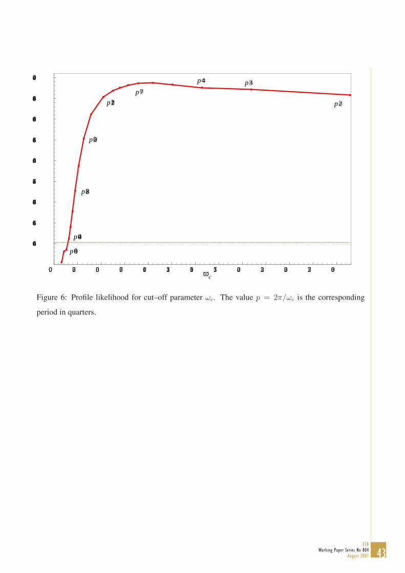
0.00 0.25 0.50 0.75 1.00 1.25 1.50 1.75 2.00 2.25 2.50 2.75 3.00

4466.0

4466.5

4467.0

4467.5

4468.0

4468.5

4469.0

4469.5

4470.0

p=2

p=3p=4p=7

p=12

p=20

p=40

p=60

p=28

ωc

Figure 6: Profile likelihood for cut–off parameter ωc. The value p = 2π/ωc is the corresponding

period in quarters.

43ECB



European Central Bank Working Paper Series

For a complete list of Working Papers published by the ECB, please visit the ECB’s website(http://www.ecb.int)

748 “Financial dollarization: the role of banks and interest rates” by H. S. Basso, O. Calvo-Gonzalez and M. Jurgilas, May 2007.

749 “Excess money growth and inflation dynamics” by B. Roffia and A. Zaghini, May 2007.

750 “Long run macroeconomic relations in the global economy” by S. Dées, S. Holly, M. H. Pesaran and L. V. Smith, May 2007.

751 “A look into the factor model black box: publication lags and the role of hard and soft data in forecasting GDP” by M. Bańbura and G. Rünstler, May 2007.

752 “Econometric analyses with backdated data: unified Germany and the euro area” by E. Angelini and M. Marcellino, May 2007.

753 “Trade credit defaults and liquidity provision by firms” by F. Boissay and R. Gropp, May 2007.

754 “Euro area inflation persistence in an estimated nonlinear DSGE model” by G. Amisano and O. Tristani, May 2007.

755 “Durable goods and their effect on household saving ratios in the euro area” by J. Jalava and I. K. Kavonius, May 2007.

756 “Maintaining low inflation: money, interest rates, and policy stance” by S. Reynard, May 2007.

757 “The cyclicality of consumption, wages and employment of the public sector in the euro area” by A. Lamo, J. J. Pérez and L. Schuknecht, May 2007.

758 “Red tape and delayed entry” by A. Ciccone and E. Papaioannou, June 2007.

759 “Linear-quadratic approximation, external habit and targeting rules” by P. Levine, J. Pearlman and R. Pierse, June 2007.

760 “Modelling intra- and extra-area trade substitution and exchange rate pass-through in the euro area” by A. Dieppe and T. Warmedinger, June 2007.

761 “External imbalances and the US current account: how supply-side changes affect an exchange rate adjustment” by P. Engler, M. Fidora and C. Thimann, June 2007.

762 “Patterns of current account adjustment: insights from past experience” by B. Algieri and T. Bracke, June 2007.

763 “Short- and long-run tax elasticities: the case of the Netherlands” by G. Wolswijk, June 2007.

764 “Robust monetary policy with imperfect knowledge” by A. Orphanides and J. C. Williams, June 2007.

765 “Sequential optimization, front-loaded information, and U.S. consumption” by A. Willman, June 2007.

766 “How and when do markets tip? Lessons from the Battle of the Bund” by E. Cantillon and P.-L. Yin, June 2007.

45ECB


767 “Explaining monetary policy in press conferences” by M. Ehrmann and M. Fratzscher, June 2007.

768 “A new approach to measuring competition in the loan markets of the euro area” by M. van Leuvensteijn, J. A. Bikker, A. van Rixtel and C. Kok Sørensen, June 2007.

769 “The ‘Great Moderation’ in the United Kingdom” by L. Benati, June 2007.

770 “Welfare implications of Calvo vs. Rotemberg pricing assumptions” by G. Lombardo and D. Vestin, June 2007.

771 “Policy rate decisions and unbiased parameter estimation in typical monetary policy rules” by J. Podpiera, June 2007.

772 “Can adjustment costs explain the variability and counter-cyclicality of the labour share at the firm and aggregate level?” by P. Vermeulen, June 2007.

773 “Exchange rate volatility and growth in small open economies at the EMU periphery” by G. Schnabl, July 2007.

774 “Shocks, structures or monetary policies? The euro area and US after 2001” by L. Christiano, R. Motto and M. Rostagno, July 2007.

775 “The dynamic behaviour of budget components and output” by A. Afonso and P. Claeys, July 2007.

776 “Insights gained from conversations with labor market decision makers” by T. F. Bewley, July 2007.

777 “Downward nominal wage rigidity in the OECD” by S. Holden and F. Wulfsberg, July 2007.

778 “Employment protection legislation and wages” by M. Leonardi and G. Pica, July 2007.

779 “On-the-job search and the cyclical dynamics of the labor market” by M. U. Krause and T. A. Lubik, July 2007.

780 “Dynamics and monetary policy in a fair wage model of the business cycle” by D. de la Croix, G. de Walqueand R. Wouters, July 2007.

781 “Wage inequality in Spain: recent developments” by M. Izquierdo and A. Lacuesta, July 2007.

782 “Panel data estimates of the production function and product and labor market imperfections” by S. Dobbelaere and J. Mairesse, July 2007.

783 “The cyclicality of effective wages within employer-employee matches: evidence from German panel data”by S. Anger, July 2007.

784 “Understanding the dynamics of labor shares and inflation” by M. Lawless and K. Whelan, July 2007.

785 “Aggregating Phillips curves” by J. Imbs, E. Jondeau and F. Pelgrin, July 2007.

786 “The economic impact of merger control: what is special about banking?” by E. Carletti, P. Hartmann and S. Ongena, July 2007.

787 “Finance and growth: a macroeconomic assessment of the evidence from a European angle” by E. Papaioannou, July 2007.

788 “Evaluating the real effect of bank branching deregulation: comparing contiguous counties across U.S. state borders” by R. R. Huang, July 2007.


789 “Modeling the impact of external factors on the euro area’s HICP and real economy: a focus on pass-through and the trade balance” by L. Landolfo, July 2007.

790 “Asset prices, exchange rates and the current account” by M. Fratzscher, L. Juvenal and L. Sarno, August 2007.

791 “Inquiries on dynamics of transition economy convergence in a two-country model” by J. Brůha and J. Podpiera, August 2007.

792 “Euro area market reactions to the monetary developments press release” by J. Coffinet and S. Gouteron, August 2007.

793 “Structural econometric approach to bidding in the main refinancing operations of the Eurosystem” by N. Cassola, C. Ewerhart and C. Morana, August 2007.

794 “(Un)naturally low? Sequential Monte Carlo tracking of the US natural interest rate” by M. J. Lombardi and S. Sgherri, August 2007.

795 “Assessing the impact of a change in the composition of public spending: a DSGE approach” by R. Straub and I. Tchakarov, August 2007.

796 “The impact of exchange rate shocks on sectoral activity and prices in the euro area” by E. Hahn, August 2007.

797 “Joint estimation of the natural rate of interest, the natural rate of unemployment, expected inflation, and potential output” by L. Benati and G. Vitale, August 2007.

798 “The transmission of US cyclical developments to the rest of the world” by S. Dées and I. Vansteenkiste, August 2007.

799 “Monetary policy shocks in a two-sector open economy: an empirical study” by R. Llaudes, August 2007.

800 “Is the corporate bond market forward looking?” by J. Hilscher, August 2007.

801 “Uncovered interest parity at distant horizons: evidence on emerging economies & nonlinearities” by A. Mehl and L. Cappiello, August 2007.

802 “Investigating time-variation in the marginal predictive power of the yield spread” by L. Benati and C. Goodhart, August 2007.

803 “Optimal monetary policy in an estimated DSGE for the euro area” by S. Adjemian, M. Darracq Paries and S. Moyen, August 2007.

804 “Growth accounting for the euro area: a structural approach” by T. Proietti and A. Musso, August 2007.

ISSN 1561081-0

9 7 7 1 5 6 1 0 8 1 0 0 5

growth accounting for the euro area: a structural approach · growth accounting for the eur o area...

Documents