group study and seminar series (summer 20) - statistics
TRANSCRIPT

Group Study and Seminar Series (Summer 20)
Statistics, Optimization and Reinforcement Learning
Yingru Li
The Chinese University of Hong Kong, Shenzhen, China
June 24, 2020
Mainly based on:
Wainwright, M. J. (2019). High-dimensional statistics: A non-asymptotic viewpoint (Vol. 48). Cambridge University Press.
Selected paper on Mathematical and Algorithmic issues in Reinforcement Learning

Outline
Introduction to the seminar series
Why Non-Asymptotic?
Basic tail and concentration bounds
Classical boundsSub-Gaussian
Sub-Exponential
Martingale based methods
Lipschitz functions of Gaussian variables
Introduction to the seminar series 2 / 82

Arrangements
I 14:00 - 17:00 in Administrative Building 603
I Every Thursday from 6/18 to 8/20
– One exception: the seminar will be held in Wednesday (6/24) next week due to the Dragon
boat festival.
– 10 weeks in total!
I Enjoy the journey!
Introduction to the seminar series 3 / 82

What to discuss and why important?
I From (theoretical) computer scientists perspective:
– “While traditional areas of computer science remain highly important, increasingly researchers
of the future will be involved with using computers to understand and extract usable
information from massive data arising in applications, not just how to make computers useful
on specific well-defined problems. With this in mind we have written this book to cover the
theory we expect to be useful in the next 40 years, just as an understanding of automata
theory, algorithms, and related topics gave students an advantage in the last 40 years. One of
the major changes is an increase in emphasis on probability, statistics, and numerical
methods.”
— Blum, A., Hopcroft, J., & Kannan, R. (2020). Foundations of data science. Cambridge
University Press.
– First chapter of the book is “High-Dimensional Space”.
– Early draft of this book with free access was used in undergrad-level and graduate-level
lectures by Cornell, Princeton, Stanford and many other US and Chinese Universities.
Introduction to the seminar series 4 / 82

What to discuss and why important?
I Fundamental tools in “High-Dimensional Statistics: A Non-Asymptotic Viewpoint” (used
for grad-level courses in UCB, MIT, Princeton, etc.)
– Basic tail and concentration bounds (week 1 and 2)
– Minimax Lower bounds (week 3)
– Uniform Law of Large Number (week 5)
– Metric Entropy and its uses (week 7)
– Random matrices (week 9)
I Potential Applications:
– Analysis of Randomized and Online Algorithms
– Statistical Learning Theory
– Statistical Signal Processing
– Differential Privacy, Random Graph Theory, (Big) Data Science
– Any subject where randomness plays an important role ...
Introduction to the seminar series 5 / 82
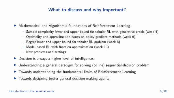
What to discuss and why important?
I Mathematical and Algorithmic foundations of Reinforcement Learning
– Sample complexity lower and upper bound for tabular RL with generative oracle (week 4)
– Optimality and approximation issues on policy gradient methods (week 6)
– Regret lower and upper bound for tabular RL problem (week 8)
– Model-based RL with function approximation (week 10)
– New problems and settings
I Decision is always a higher-level of intelligence.
I Understanding a general paradigm for solving (online) sequential decision problem
I Towards understanding the fundamental limits of Reinforcement Learning
I Towards designing better general decision-making agents
Introduction to the seminar series 6 / 82

Outline
Introduction to the seminar series
Why Non-Asymptotic?
Basic tail and concentration bounds
Classical boundsSub-Gaussian
Sub-Exponential
Martingale based methods
Lipschitz functions of Gaussian variables
Introduction to the seminar series 7 / 82

Data matrix
I A good example to keep in mind is a dataset organized as an n by d matrix X where,
– for example, the rows correspond to patients and,
– the columns correspond to measurements on each patient (height, weight, heart rate, . . . ).
I Row i is a random vector X>i ∈ Rd of the measurements performed on patient i.
X =
X>1X>2
...
X>n
∈ Rn×d
I Modern applications in science and engineering:
– large-scale problems: both d and n may be large (possibly d� n)
– need for high-dimensional theory that provides non-asymptotic results for (n, d)
Introduction to the seminar series 8 / 82
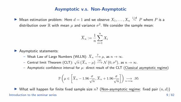
Asymptotic v.s. Non-Asymptotic
I Mean estimation problem: Here d = 1 and we observe X1, . . . , Xni.i.d∼ P where P is a
distribution over R with mean µ and variance σ2. We consider the sample mean:
Xn :=1
n
n∑i=1
Xi
I Asymptotic statements:
– Weak Law of Large Numbers (WLLN): XnP−→ µ, as n→∞.
– Central limit Theorem (CLT):√n(Xn − µ
) (d)−→ N(0, σ2
), as n→∞.
– Asymptotic confidence interval for µ: direct result of the CLT (Classical asymptotic regime)
P(µ ∈
[Xn − 1.96
σ√n,Xn + 1.96
σ√n
])−→n→∞
.95
I What will happen for finite fixed sample size n? (Non-asymptotic regime: fixed pair (n, d))
Introduction to the seminar series 9 / 82

Asymptotic v.s. Non-Asymptotic
I Asymptotic statements: Asymptotic confidence interval for µ
P(µ ∈
[Xn − 1.96
σ√n,Xn + 1.96
σ√n
])−→n→∞
.95
I Non-asymptotic statements:
– Quadratic risk: E[(Xn − µ
)2]= σ2
n
– Tail bounds: P(∣∣Xn − µ
∣∣ > t)≤ 2e−Cnt
2
, where C > 0 is a constant that depends on
further assumptions on P, such as having a bounded support (Hoeffding’s inequality)
– Non-Asymptotic confidence interval for µ: result of Hoeffding’s inequality
P(µ ∈
[Xn − C
σ√n,Xn + C
σ√n
])≥ .95
where C is a constant typically larger than 1.96.
Introduction to the seminar series 10 / 82

Asymptotic v.s. Non-Asymptotic
I Covariance matrix estimation: assume now that we observe X1, . . . , Xni.i.d∼ P
– where P is a distribution over Rd with zero mean and covariance matrix
Σ = cov(X1) = E[X1X
>1
]. The sample covariance matrix Σ is defined as
Σ :=
average of d× d rank one matrices︷ ︸︸ ︷1
n
n∑k=1
XkX>k , with E
(Σ)= Σ,
Var(Σi,j
)= E
(Σi,j −Σi,j
)2=
1
n2
n∑k=1
E (Xk,iXk,j −Σi,j)2 =
1
nVar (X1,iX1,j)
I Asymptotic statements:
– WLLN: Σi,jP−→ Σi,j , for all i, j = 1, . . . , d as n→∞
– CLT:√n(Σi,j −Σi,j
)(d)−→ N (0,Var (X1,iX1,j)) as n→∞
– In this case, letting n→∞ implicitly assumes that n� d. But what if n is of the order of d
or even if n� d?Introduction to the seminar series 11 / 82
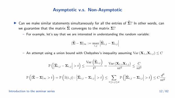
Asymptotic v.s. Non-Asymptotic
I Can we make similar statements simultaneously for all the entries of Σ? In other words, can
we guarantee that the matrix Σ converges to the matrix Σ?
– For example, let’s say that we are interested in understanding the random variable:
|Σ−Σ|∞ := maxi,j
∣∣∣Σi,j −Σi,j
∣∣∣– An attempt using a union bound with Chebyshev’s inequality assuming Var (X1,iX1,j) ≤ C
P(∣∣∣Σi,j −Σi,j
∣∣∣ > t)≤
Var(Σi,j
)t2
=Var (X1,iX1,j)
nt2≤ C
nt2
P(|Σ−Σ|∞ > t
)= P
(∃(i, j) :
∣∣∣Σi,j −Σi,j
∣∣∣ > t)≤
∑1≤i,j≤d
P(∣∣∣Σi,j −Σi,j
∣∣∣ > t)≤ C d2
nt2
Introduction to the seminar series 12 / 82
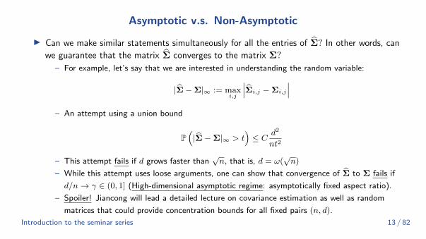
Asymptotic v.s. Non-Asymptotic
I Can we make similar statements simultaneously for all the entries of Σ? In other words, can
we guarantee that the matrix Σ converges to the matrix Σ?
– For example, let’s say that we are interested in understanding the random variable:
|Σ−Σ|∞ := maxi,j
∣∣∣Σi,j −Σi,j
∣∣∣– An attempt using a union bound
P(|Σ−Σ|∞ > t
)≤ C d2
nt2
– This attempt fails if d grows faster than√n, that is, d = ω(
√n)
– While this attempt uses loose arguments, one can show that convergence of Σ to Σ fails if
d/n→ γ ∈ (0, 1] (High-dimensional asymptotic regime: asymptotically fixed aspect ratio).
– Spoiler! Jiancong will lead a detailed lecture on covariance estimation as well as random
matrices that could provide concentration bounds for all fixed pairs (n, d).
Introduction to the seminar series 13 / 82
Asymptotic v.s. Non-Asymptotic
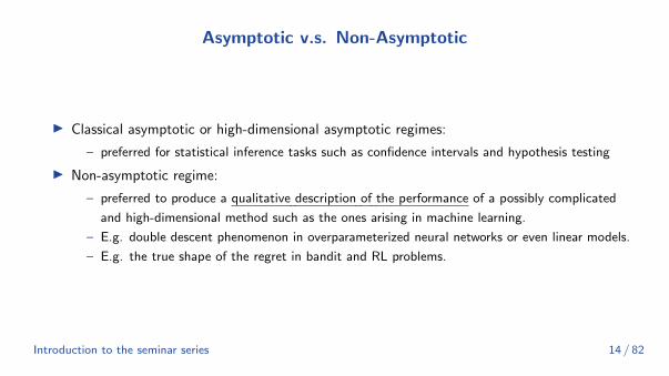
I Classical asymptotic or high-dimensional asymptotic regimes:
– preferred for statistical inference tasks such as confidence intervals and hypothesis testing
I Non-asymptotic regime:
– preferred to produce a qualitative description of the performance of a possibly complicated
and high-dimensional method such as the ones arising in machine learning.
– E.g. double descent phenomenon in overparameterized neural networks or even linear models.
– E.g. the true shape of the regret in bandit and RL problems.
Introduction to the seminar series 14 / 82

Outline
Introduction to the seminar series
Why Non-Asymptotic?
Basic tail and concentration bounds
Classical boundsSub-Gaussian
Sub-Exponential
Martingale based methods
Lipschitz functions of Gaussian variables
Basic tail and concentration bounds 15 / 82

Outline
Introduction to the seminar series
Why Non-Asymptotic?
Basic tail and concentration bounds
Classical boundsSub-Gaussian
Sub-Exponential
Martingale based methods
Lipschitz functions of Gaussian variables
Basic tail and concentration bounds 16 / 82
Mills Ratio Inequality
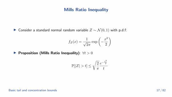
I Consider a standard normal random variable Z ∼ N (0, 1) with p.d.f:
fZ(x) =1√2π
exp
(−x
2
2
)I Proposition (Mills Ratio Inequality): ∀t > 0
P[|Z| > t] ≤√
2
π
e−t2
2
t
Basic tail and concentration bounds 17 / 82
Proof of Mills Ratio
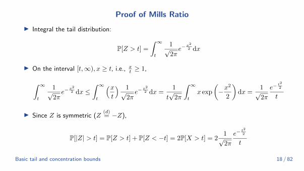
I Integral the tail distribution:
P[Z > t] =
∫ ∞t
1√2πe−
x2
2 dx
I On the interval [t,∞), x ≥ t, i.e., xt ≥ 1,
∫ ∞t
1√2πe−
x2
2 dx ≤∫ ∞t
(xt
) 1√2πe−
x2
2 dx =1
t√
2π
∫ ∞t
x exp
(−x
2
2
)dx =
1√2π
e−t2
2
t
I Since Z is symmetric (Z(d)= −Z),
P[|Z| > t] = P[Z > t] + P[Z < −t] = 2P[X > t] = 21√2π
e−t2
2
t
Basic tail and concentration bounds 18 / 82
Motivation
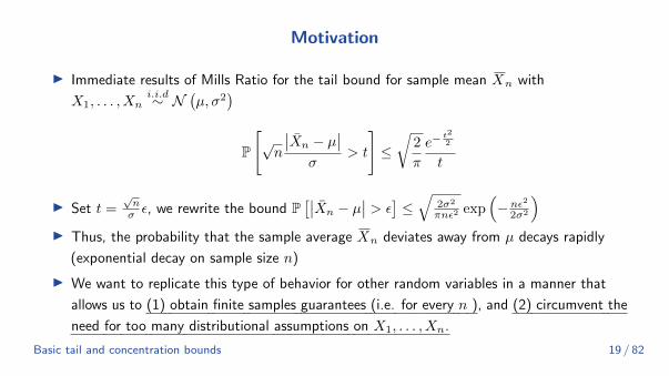
I Immediate results of Mills Ratio for the tail bound for sample mean Xn with
X1, . . . , Xni.i.d∼ N
(µ, σ2
)P
[√n
∣∣Xn − µ∣∣
σ> t
]≤√
2
π
e−t2
2
t
I Set t =√nσ ε, we rewrite the bound P
[∣∣Xn − µ∣∣ > ε
]≤√
2σ2
πnε2 exp(− nε2
2σ2
)I Thus, the probability that the sample average Xn deviates away from µ decays rapidly
(exponential decay on sample size n)
I We want to replicate this type of behavior for other random variables in a manner that
allows us to (1) obtain finite samples guarantees (i.e. for every n ), and (2) circumvent the
need for too many distributional assumptions on X1, . . . , Xn.
Basic tail and concentration bounds 19 / 82
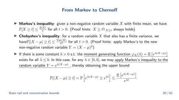
From Markov to Chernoff
I Markov’s inequality: given a non-negative random variable X with finite mean, we have
P[X ≥ t] ≤ E[X]t for all t > 0. (Proof hints: X ≥ t1X≥t always holds)
I Chebyshev’s inequality: for a random variable X that also has a finite variance, we
haveP[|X − µ| ≥ t] ≤ Var(X)t2 for all t > 0. (Proof hints: apply Markov’s to the new
non-negative random variable Y = (X − µ)2)
I If there is some constant b > 0 s.t. the moment generating function ϕX(λ) = E[eλ(X−µ)
]exists for all λ ≤ b. In this case, for any λ ∈ [0, b], we may apply Markov’s inequality to the
random variable Y = eλ(X−µ) , thereby obtaining the upper bound
P[(X − µ) ≥ t] = P[eλ(X−µ) ≥ eλt
]≤
E[eλ(X−µ)
]eλt
Basic tail and concentration bounds 20 / 82
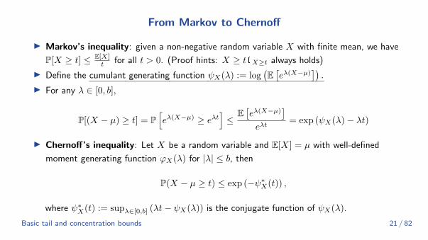
From Markov to Chernoff
I Markov’s inequality: given a non-negative random variable X with finite mean, we have
P[X ≥ t] ≤ E[X]t for all t > 0. (Proof hints: X ≥ t1X≥t always holds)
I Define the cumulant generating function ψX(λ) := log(E[eλ(X−µ)
]).
I For any λ ∈ [0, b],
P[(X − µ) ≥ t] = P[eλ(X−µ) ≥ eλt
]≤
E[eλ(X−µ)
]eλt
= exp (ψX(λ)− λt)
I Chernoff’s inequality: Let X be a random variable and E[X] = µ with well-defined
moment generating function ϕX(λ) for |λ| ≤ b, then
P(X − µ ≥ t) ≤ exp (−ψ∗X(t)) ,
where ψ∗X(t) := supλ∈[0,b] (λt− ψX(λ)) is the conjugate function of ψX(λ).
Basic tail and concentration bounds 21 / 82

Chernoff bound for Gaussian
I Let X ∼ N(µ, σ2
), then E
[eλX
]= eµλ+σ2λ2/2 for all λ ∈ R. So, we have
supλ≥0
(λt− log
(E[eλ(X−µ)
]))= sup
λ≥0
(λt− λ2σ2
2
)=
t2
2σ2
which yields the bound for all t > 0,
P (X − µ ≥ t) ≤ exp
(−t2
2σ2
)I This bound is sharp up to polynomial-factor corrections, compared to the Mills Ratio.
I Deriving a Chernoff bound does not require less knowledge about a distribution than a
Markov-based bound since we need the moment generating function of X − µ. (Assume the
existence of infinity many moments)
I A main advantage is that these moments do not have to be painstakingly calculated.Basic tail and concentration bounds 22 / 82

Sub-Gaussian random variables
I Definition (Sub-Gaussian random variables): A random variable X is Sub-Gaussian
with parameter σ if
E[eλ(X−E[X])
]≤ exp
(λ2σ2
2
)for all λ ∈ R. In that case, we write X ∈ SG
(σ2).
I First simple observation: X ∈ SG(σ2)
iff −X ∈ SG(σ2).
I Second observation: if X ∈ SG(σ2), then the MGF of X can be bounded by the Gaussian
MGF which yields the same Chernoff bound, i. e.
P(|X − µ| ≥ t) ≤ 2 exp
(−t2
2σ2
)
Basic tail and concentration bounds 23 / 82

Properties of Sub-Gaussian random variables
I Let X ∈ SG(σ2), then Var[X] ≤ σ2 with Var[X] = σ2 if X is Gaussian.
I If there are a, b ∈ R such that a ≤ X − µ ≤ b almost everywhere, then X ∈ SG((
b−a2
)2)I Let X ∈ SG
(σ2)
and Y ∈ SG(τ2), then
– Xα ∈ SG(σ2α2
)for all α ∈ R with α 6= 0
– X + Y ∈ SG((τ + σ)2
), and
– if X ⊥ Y,X + Y ∈ SG(τ2 + σ2
)
Basic tail and concentration bounds 24 / 82
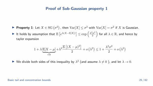
Proof of Sub-Gaussian property 1
I Property 1: Let X ∈ SG(σ2), then Var[X] ≤ σ2 with Var[X] = σ2 if X is Gaussian.
I It holds by assumption that E[eλ(X−E[X])
]≤ exp
(λ2σ2
2
)for all λ ∈ R, and hence by
taylor expansion
1 + λE[X − µ]︸ ︷︷ ︸=0
+λ2E[(X − µ)2
]2
+ o(λ2)≤ 1 +
λ2σ2
2+ o
(λ2)
I We divide both sides of this inequality by λ2 (and assume λ 6= 0 ), and let λ→ 0.
Basic tail and concentration bounds 25 / 82

Proof of Sub-Gaussian property 2
I Property 2: If there are a, b ∈ R such that a ≤ X − µ ≤ b almost everywhere, then
X ∈ SG((
b−a2
)2)I W.L.O.G, let µ = 0. We need to show that log
(E[eλX
])≤ (b−a)2λ2
8 for all λ ∈ R.I First, notice that for any distribution supported on [a, b], the variance
Var[X] = E(X − E(X))2 ≤ E(X − (a+ b)/2)2︸ ︷︷ ︸E(X)=arg mins g(s):=E(X−s)2
= 14E((X − a)︸ ︷︷ ︸
≥0
+ (X − b)︸ ︷︷ ︸≤0
)2 ≤(b−a
2
)2.
I Remind the CGF ψX(λ) = logE[eλX
], and ψX(0) = 0. Define a new prob. measure:
P(A) =
∫AeλxP(dx)∫eλyP(dy)
I We have the derivatives: ψ′X(λ) =E[XeλX ]E[eλX ]
= EP(X). Note that ψ′X(0) = EP(0) = 0.
Basic tail and concentration bounds 26 / 82
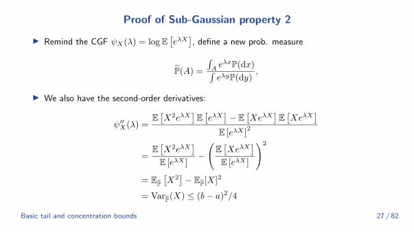
Proof of Sub-Gaussian property 2
I Remind the CGF ψX(λ) = logE[eλX
], define a new prob. measure
P(A) =
∫AeλxP(dx)∫eλyP(dy)
,
I We also have the second-order derivatives:
ψ′′X(λ) =E[X2eλX
]E[eλX
]− E
[XeλX
]E[XeλX
]E [eλX ]
2
=E[X2eλX
]E [eλX ]
−
(E[XeλX
]E [eλX ]
)2
= EP[X2]− EP[X]2
= VarP(X) ≤ (b− a)2/4
Basic tail and concentration bounds 27 / 82

Proof of Sub-Gaussian property 2
I Property 2: If there are a, b ∈ R such that a ≤ X − µ ≤ b almost everywhere, then
X ∈ SG((
b−a2
)2)I ψX(0) = ψ′X(0) = 0 and ψ′′X(λ) ≤ (b− a)2/4 for all λ.
I The fundamental theorem of calculus:
ψX(λ) =
∫ λ
0
ψ′X(u)du =
∫ λ
0
∫ u
0
ψ′′X(w)dwdu ≤∫ λ
0
∫ u
0
(b− a)2
4dwdu = λ2 (b− a)2
8
I This result can be used to prove Hoeffding’s bound.
Basic tail and concentration bounds 28 / 82

I Property 3: Let X ∈ SG(σ2)
and Y ∈ SG(τ2), then
i Xα ∈ SG(σ2α2
)for all α ∈ R with α 6= 0
ii X + Y ∈ SG((τ + σ)2
), and
iii if X ⊥ Y,X + Y ∈ SG(τ2 + σ2
)I We prove (ii) and (iii) and assume that E[X] = E[Y ]. If X ⊥ Y , the proof is immediate. If
not, it holds for every λ ∈ R that E[eλ(X+Y )
]= E
[eλXeλY
]. By Holder’s inequality,
E[eλ(X+Y )
]= E
[eλXeλY
]≤(E[eλpX
])1/p (E [eλqY ])1/qSG≤ exp
(λ2p2σ2
2
1
p+λ2q2τ2
2
1
q
)= exp
(λ2
2
(pσ2 + qτ2
))= exp
(λ2
2(σ + τ)2
)where we set p = (τ + σ)/σ in the last step.
Basic tail and concentration bounds 29 / 82
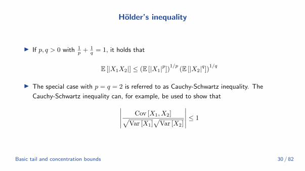
Holder’s inequality
I If p, q > 0 with 1p + 1
q = 1, it holds that
E [|X1X2|] ≤ (E [|X1|p])1/p
(E [|X2|q])1/q
I The special case with p = q = 2 is referred to as Cauchy-Schwartz inequality. The
Cauchy-Schwartz inequality can, for example, be used to show that∣∣∣∣∣ Cov [X1, X2]√Var [X1]
√Var [X2]
∣∣∣∣∣ ≤ 1
Basic tail and concentration bounds 30 / 82

Hoeffding inequality
I Theorem (Hoeffding inequality): LetX1, . . . , Xn be independent random variables such
that Xi ∈ SG(σ2i
)for all i, then
P
(∣∣∣∣∣n∑i=1
Xi − E [Xi]
n
∣∣∣∣∣ ≥ t)≤ 2 exp
(−n2t2
2∑ni=1 σ
2i
)
I Usually, we have σ2i = σ2 for all i. In this case, it holds that
2 exp
(−n2t2
2∑ni=1 σ
2i
)= 2 exp
(−nt2
2σ2
)I The proof is trivial using the properties of Sub-Gaussian.
Basic tail and concentration bounds 31 / 82

I Example (Hoeffding for Bernoulli R.V. ): LetX1, . . . , Xn be independent R.V. with
Xi ∼ Bernoulli(pi) for some pi ∈ (0, 1). Then, Xi ∈ SG(1/4) and thus
P(∣∣Xn − pn
∣∣ ≥ t) ≤ 2 exp(−2nt2
)where Xn := 1
n
∑ni=1Xi and pn := 1
n
∑ni=1 pi. Thus, we have that
∣∣Xn − pn∣∣ ≤√ 1
2nlog
(1
δ
)with probability at least 1− δ.
I In the case X1, . . . , Xniid∼ Bernoulli (p). Set δ = 1
nc for some c > 0. For example, we have
that with probability at least 1− 1n ,
∣∣Xn − p∣∣ ≤√ 1
2nlog(2n) = O
(√log n
n
)= O
(1√n
)Basic tail and concentration bounds 32 / 82

Comparing Hoeffding and Chernoff Bounds
I Hoeffding’s inequality is not the sharpest concentration inequality in general. Note that the
above calculations would similarly hold for any bounded random variable.
I Chernoff’s multiplicative inequality yields an improvement on Hoeffding’s inequality ’
whenever p is small. Generally for Xi ∼ Bernoulli (pi) for some pi ∈ (0, 1),
P
{n∑i=1
Xi ≥ (1 + ε)
n∑i=1
pi
}≤
exp{− ε
2 ∑ni=1 pi3
}, ε ∈ (0, 1]
exp{− ε
2 ∑ni=1 pi
2+ε
}, ε > 1
,
and
P
{n∑i=1
Xi ≤ (1− ε)n∑i=1
pi
}≤ exp
{−ε2∑ni=1 pi2
}, ∀ε ∈ (0, 1)
Basic tail and concentration bounds 33 / 82

Comparing Hoeffding and Chernoff Bounds
I Let X1, . . . , Xniid∼ Bernoulli(p). Hoeffding’s inequality gave, w. p. at least 1− δ.
p− Xn ≤√
12n log(1/δ)
I On the other hand, Chernoff’s multiplicative inequality yields
P{p− Xn ≥ εp
}≤ exp
(−npε
2
2
), ∀ε ∈ (0, 1)
I Provided p ≥ 2n log(1/δ), we have p− Xn ≤
√2pn log(1/δ) w.p. 1− δ
I If we let p ≡ pn so that pn → 0, then Chernoff’s provides a significant improvement upon
Hoeffding’s.
– Because the variance is upper bounded by p(1− p), which is shrinking as the sample size
grows. Chernoff’s multiplicative inequality incorporates this information.
Basic tail and concentration bounds 34 / 82

Equivalent Definitions of Sub-Gaussian Random Variables
I Proposition. Let Γ(x) =∫∞
0tx−1e−tdt be the Gamma function. If X ∈ SG
(σ2),
E [|X|p] ≤ p2p/2σpΓ(p/2), ∀p > 0
In particular, there exists C > 0 not depending on p such that
(E [|X|p])1p ≤ Cσ√p.
I Remark. For example, if X ∼ N(0, σ2
), we have
E [|X|p] =σp2
p2 Γ(p+1
2
)√π
Basic tail and concentration bounds 35 / 82

Proof of the equivalent definition
I If x ≥ 0 then x =∫ x
0dt =
∫∞0
I[t ≤ x]dt. Using Fubini’s theorem, (p-th order moment
exists due to Sub-Gaussianess)
E [|X|p] =
∫ ∞0
P (|X|p ≥ u) du =
∫ ∞0
P(|X| ≥ u
1p
)du ≤ 2
∫ ∞0
exp
{−u
2/p
2σ2
}du
≤ 2(2σ2) p
2p
2
∫ ∞0
e−ttp2−1dt︸ ︷︷ ︸
Γ( p2 )
(where t =
u2p
2σ2
)
=(2σ2) p
2 pΓ(p
2
)≤(2σ2) p
2 p(p
2
)p/2I ‖X‖p := (E [|X|p])
1p ≤ p1/pσ
√p ≤ Cσ√p, since we can optimize fn. p1/p over p.
Basic tail and concentration bounds 36 / 82

Laplace distribution
I Example Let X ∼ Laplace (0, b) for b > 0. Then it can be shown that
P(|X| ≥ t) ≤ exp(−tb), ∀t > 0
I The Laplace distribution has fatter tails than the normal distribution
Basic tail and concentration bounds 37 / 82
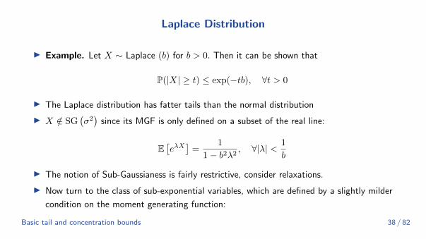
Laplace Distribution
I Example. Let X ∼ Laplace (b) for b > 0. Then it can be shown that
P(|X| ≥ t) ≤ exp(−tb), ∀t > 0
I The Laplace distribution has fatter tails than the normal distribution
I X /∈ SG(σ2)
since its MGF is only defined on a subset of the real line:
E[eλX
]=
1
1− b2λ2, ∀|λ| < 1
b
I The notion of Sub-Gaussianess is fairly restrictive, consider relaxations.
I Now turn to the class of sub-exponential variables, which are defined by a slightly milder
condition on the moment generating function:
Basic tail and concentration bounds 38 / 82

Sub-Exponential Random Variable
I Definition (Sub-Exponential Random Variable). We say that a random variable X is
Sub-Exponential with parameters ν, α > 0, and we write X ∈ SE(ν2, α
), if
E[eλ(X−E(X))
]≤ eλ
2ν2
2 , ∀|λ| < 1
α
I Remark. An immediate consequence of the definition is that SG(σ2)⊆ SE
(σ2, 0
). Thus,
all Sub-Gaussian random variables are also Sub-Exponential.
Basic tail and concentration bounds 39 / 82

Chi-square distribution
I Example. Let Z ∼ N (0, 1), and X = Z2 ∼ χ2(1),E(X) = 1. Let λ < 1
2 . Then
E[eλ(X−1)
]=
1√2πe−λ
∫ ∞−∞
e−z2
2 (1−2λ)dz
= e−λ1√
1− 2λ
1√2π
∫ ∞−∞
e−y2
2 dy(y = z
√1− 2λ
)=
e−λ√1− 2λ
(a)
≤ exp
{λ2
1− 2λ
}(b)
≤ exp
{4λ2
2
} (λ <
1
4
)I Thus, X ∈ SE(4, 4). The inequality (a) follows from the following elementary inequality
− log(1− u)− u ≤ u2
2(1−u) ,∀u ∈ (0, 1) with u = 2λ. And (b) is due to the chosen λ < 1/4.
I Also, it is possible to show that P(X − 1 > 2t+ 2√t) ≤ e−t,∀t > 0
Basic tail and concentration bounds 40 / 82

Tail Bounds for Sub-Exponential Random Variables
I Theorem. Let X ∈ SE(ν2, α
), and t > 0. Then
P{X − E(X) ≥ t} ≤
{exp
{− t2
2ν2
}, t ≤ ν2
α (Sub-Gaussian behavior)
exp{− t
2α
}, t > ν2
α
Equivalently,
P{X − E(X) ≥ t} ≤ exp
{−1
2min
(t2
ν2,t
α
)}
Basic tail and concentration bounds 41 / 82
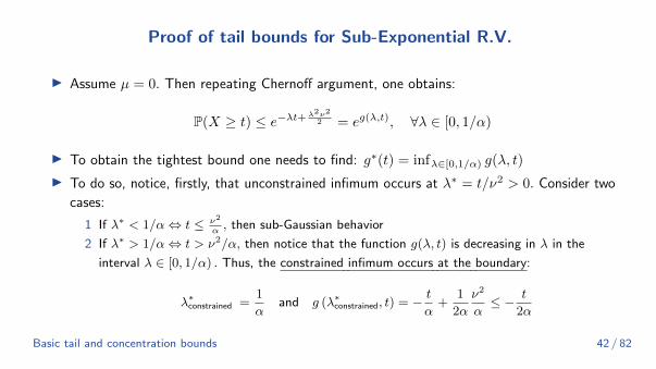
Proof of tail bounds for Sub-Exponential R.V.
I Assume µ = 0. Then repeating Chernoff argument, one obtains:
P(X ≥ t) ≤ e−λt+λ2ν2
2 = eg(λ,t), ∀λ ∈ [0, 1/α)
I To obtain the tightest bound one needs to find: g∗(t) = infλ∈[0,1/α) g(λ, t)
I To do so, notice, firstly, that unconstrained infimum occurs at λ∗ = t/ν2 > 0. Consider two
cases:
1 If λ∗ < 1/α⇔ t ≤ ν2
α, then sub-Gaussian behavior
2 If λ∗ > 1/α⇔ t > ν2/α, then notice that the function g(λ, t) is decreasing in λ in the
interval λ ∈ [0, 1/α) . Thus, the constrained infimum occurs at the boundary:
λ∗constrained =1
αand g (λ∗constrained, t) = −
t
α+
1
2α
ν2
α≤ − t
2α
Basic tail and concentration bounds 42 / 82

Bernstein condition
I Recall that sufficient conditions for a random variable to be a Sub-Gaussian include:
– Boundedness of a random variable
– Condition on the moments(E|X|k
)1/kI Bernstein condition is one similar condition allowing unbounded random variables to behave
sub-exponentially.
I Definition (Bernstein condition). Let X be a random variable with mean µ and variance
σ2. Assume that ∃b > 0,
E|X − µ|k ≤ 1
2k!σ2bk−2, k = 3, 4, . . .
Then one says that X satisfies Bernstein condition.
Basic tail and concentration bounds 43 / 82
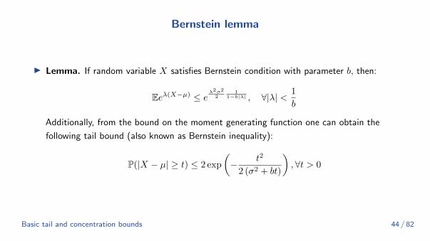
Bernstein lemma
I Lemma. If random variable X satisfies Bernstein condition with parameter b, then:
Eeλ(X−µ) ≤ eλ2σ2
21
1−b|λ| , ∀|λ| < 1
b
Additionally, from the bound on the moment generating function one can obtain the
following tail bound (also known as Bernstein inequality):
P(|X − µ| ≥ t) ≤ 2 exp
(− t2
2 (σ2 + bt)
),∀t > 0
Basic tail and concentration bounds 44 / 82

Proof of Bernstein lemma
I Pick λ : |λ| < 1b (allowing interchanging summation and taking expectation) and expand
the MGF in a Taylor series:
Eeλ(X−µ) = 1 +λ2σ2
2+
∞∑k=3
E|X − µ|k
k!λk ≤ 1 +
λ2σ2
2+λ2σ2
2
∞∑k=3
(|λ|b)k−2
= 1 +λ2σ2
2
1
1− b|λ|≤ e
λ2σ2
21
1−b|λ| , (1 + x ≤ ex)
I To show the final bound, take λ : |λ| < 12b . Then the bound becomes:
eλ2σ2
21
1−b|λ| ≤ eλ2σ2
= eλ2(2σ2)
2 =⇒ X ∈ SE(2σ2, 2b
).
I The concentration result follows by taking λ = tbt+σ2 ∈ [0, 1
b ) in the Chernoff bound.
Basic tail and concentration bounds 45 / 82

Proof of the Bernstein lemma
I The concentration result follows by taking λ = tbt+σ2 ∈ [0, 1
b ) in the Chernoff bound.
P[X − µ ≥ t] ≤ exp
(λ2σ2
2(1− b|λ|)− λt
)
= exp
(
tbt+σ2
)2
σ2
2σ2
bt+σ2
− t2
bt+ σ2
= exp
(− t2
2(bt+ σ2)
)
Basic tail and concentration bounds 46 / 82
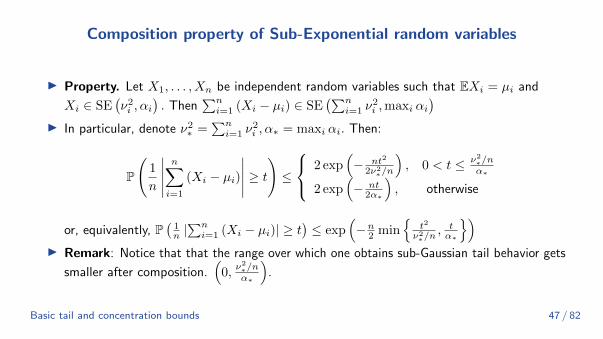
Composition property of Sub-Exponential random variables
I Property. Let X1, . . . , Xn be independent random variables such that EXi = µi and
Xi ∈ SE(ν2i , αi
). Then
∑ni=1 (Xi − µi) ∈ SE
(∑ni=1 ν
2i ,maxi αi
)I In particular, denote ν2
∗ =∑ni=1 ν
2i , α∗ = maxi αi. Then:
P
(1
n
∣∣∣∣∣n∑i=1
(Xi − µi)
∣∣∣∣∣ ≥ t)≤
2 exp(− nt2
2ν2∗/n
), 0 < t ≤ ν2
∗/nα∗
2 exp(− nt
2α∗
), otherwise
or, equivalently, P(
1n |∑ni=1 (Xi − µi)| ≥ t
)≤ exp
(−n2 min
{t2
ν2∗/n
, tα∗
})I Remark: Notice that that the range over which one obtains sub-Gaussian tail behavior gets
smaller after composition.(
0,ν2∗/nα∗
).
Basic tail and concentration bounds 47 / 82

Orlicz norm
I Definition (ψ-Orlicz norm). Let function ψ : R+ → R+ satisfy the following properties:
– ψ(x) is strictly increasing function
– ψ(x) is a convex function
– ψ(0) = 0
Then the ψ-Orlicz norm of a random variable X is defined as
‖X‖ψ = inf
{t > 0 : Eψ
(|X|t
)≤ 1
}I Example 1. Let ψ(x) = xp, p ≥ 1. Then:
‖X‖ψ = ‖X‖p = (E|X|p)1p
Basic tail and concentration bounds 48 / 82

Orlicz norm
I Example 2. Let ψp(x) = exp − 1, p ≥ 1. The corresponding Orlicz has two properties:
(a) p = 1 : then ‖X‖ψ1 <∞ is equivalent to X belonging to the class of Sub-Exponential
random variables
(b) p = 2 : then ‖X‖ψ2 <∞ is equivalent to X belonging to the class of Sub-Gaussian random
variables
I It is easy to show that (by definition):∥∥X2∥∥ψ1
= (‖X‖ψ2)2, ‖XY ‖ψ1 ≤ ‖X‖ψ2‖Y ‖ψ2
I Using Orlicz norms allows to straightforwardly implies the following facts:
1 Squared Sub-Gaussian random variable is Sub-Exponential.
2 Product of two Sub-Gaussian random variables is Sub-Exponential.
Basic tail and concentration bounds 49 / 82

Concentraiton of a sub-gaussian random vector
I Lemma (Concentration of a sub-gaussian random vector) Let
X = (X1, . . . , Xd)> ∈ Rd be such that: EXi = 0,V (Xi) = 1 and assume that
Xi ∈ SG (1) . Then we can show that ‖X‖2 concentrates around√d.
I Proof:
– Consider ‖X‖22 =∑ni=1X
2i . Then X2
i − 1 ∈ SE(ν2, α
)Thus, we have
P(∣∣∣ ‖X‖2d
− 1∣∣∣ ≥ t) ≤ 2 exp
(− d
2min
{t2
ν2 ,tα
}), ∀t > 0
– We will need to use the following fact: fix c > 0. Then for any numbers z > 0,
|z − 1| ≥ c implies=⇒ z2 − 1 ≥ max
{c, c2
}.
P(∣∣∣∣‖X‖√d − 1
∣∣∣∣ ≥ u) ≤ P(∣∣∣∣‖X‖2d
− 1
∣∣∣∣ ≥ max{u, u2}) ≤ 2 exp
(−du
2
2C
)I See more modern discussions on concentration of random vector in [Jin, Netrapalli, Ge,
Kakade, and Jordan, 2019].
Basic tail and concentration bounds 50 / 82

Hoeffding vs. Bernstein
I One would like to compare two type of bounds/inequalities: Hoeffding’s and Bernstein’s.
Denote µ = EX andσ2 = V(X). Assume that |X − µ| ≤ b a.e. Then:
P(|X − µ| ≥ t) ≤
2 exp(− t2
2b2
), Hoeffding
2 exp(− t2
2(σ2+bt)
), Bernstein
I For small t (meaning bt� σ2 ) Bernstein’s inequality gives rise to a bound of the order:
P(|X − µ| ≥ t) ≤ 2e−t2
cσ2 while Hoeffding’s gives: P(|X − µ| ≥ t) ≤ 2e−t2
cb2
I But σ2 ≤ b2 and, thus, Bernstein’s bound is tighter. Substantially tighter when σ2 � b2.
– The case for a random variable that occasionally takes on large values.
– (Further strengthen) For bounded R.V., Bennett’s inequality is sharper then Bernstein’s.
Basic tail and concentration bounds 51 / 82
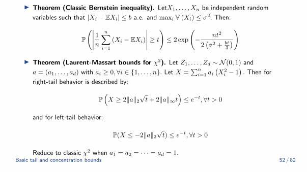
I Theorem (Classic Bernstein inequality). LetX1, . . . , Xn be independent random
variables such that |Xi − EXi| ≤ b a.e. and maxiV (Xi) ≤ σ2. Then:
P
(∣∣∣∣∣ 1nn∑i=1
(Xi − EXi)
∣∣∣∣∣ ≥ t)≤ 2 exp
(− nt2
2(σ2 + bt
3
))
I Theorem (Laurent-Massart bounds for χ2). Let Z1, . . . , Zd ∼ N (0, 1) and
a = (a1, . . . , ad) with ai ≥ 0,∀i ∈ {1, . . . , n}. Let X =∑ni=1 ai
(X2i − 1
). Then for
right-tail behavior is described by:
P(X ≥ 2‖a‖2
√t+ 2‖a‖∞t
)≤ e−t,∀t > 0
and for left-tail behavior:
P(X ≤ −2‖a‖2√t) ≤ e−t,∀t > 0
Reduce to classic χ2 when a1 = a2 = · · · = ad = 1.Basic tail and concentration bounds 52 / 82

Johnson–Lindenstrauss embedding
I Suppose that we are given N ≥ 2 distinct vectors{u1, . . . , uN
}, with each vector in Rd.
I The data dimension d is large. Expensive to store and manipulate the data set.
I The idea of dimensionality reduction is to construct a mapping F : Rd → Rm
I Want mapping F satisfies
(1) the projected dimension
m� d
(2) mapping F preserves pairwise distances, or equivalently norms and inner products.
I Many ML algorithms are based on such pairwise quantities, including (1) linear regression,
(2) methods for principal components, (3) the k -means algorithm for clustering, and (4)
nearest-neighbor algorithms for density estimation.
Basic tail and concentration bounds 53 / 82

Johnson–Lindenstrauss embedding
I Suppose that we are given N ≥ 2 distinct vectors{u1, . . . , uN
}, with each vector in Rd.
I The data dimension d is large. Expensive to store and manipulate the data set.
I The idea of dimensionality reduction is to construct a mapping F : Rd → Rm
I more precisely, given some tolerance δ ∈ (0, 1), we might be interested in a mapping F
with the guarantee that
(1− δ) ≤∥∥F (ui)− F (uj)∥∥2
2
‖ui − uj‖22≤ (1 + δ) for all pairs ui 6= uj (1)
Basic tail and concentration bounds 54 / 82

Johnson–Lindenstrauss embedding
I An interesting and simple construction of the mapping that satisfies the condition 1 is
probabilistic (known as Johnson–Lindenstrauss embedding or Random Projection):
– Form a random matrix X ∈ Rm×d filled with independent N (0, 1) entries
– and use it to define a linear mapping
F : Rd → Rm via u 7→ Xu/√m
I Random projection satisfies the condition 1 with high probability as long as the projected
dimension is lower bounded as
m %1
δ2logN.
– The projected dimension m is independent of the ambient dimension d, and scales only
logarithmically with the number of data points N .
Basic tail and concentration bounds 55 / 82
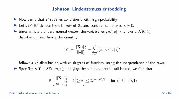
Johnson–Lindenstrauss embedding
I Now verify that F satisfies condition 1 with high probability.
I Let xi ∈ Rd denote the i th row of X, and consider some fixed u 6= 0.
I Since xi is a standard normal vector, the variable 〈xi, u/‖u‖2〉 follows a N (0, 1)
distribution, and hence the quantity
Y :=‖Xu‖22‖u‖22
=
m∑i=1
〈xi, u/‖u‖2〉2
follows a χ2 distribution with m degrees of freedom, using the independence of the rows.
I Specifically Y ∈ SE(4m, 4), applying the sub-exponential tail bound, we find that
P[∣∣∣∣ ||Xu‖22m‖u‖22
− 1
∣∣∣∣ ≥ δ] ≤ 2e−mδ2/8 for all δ ∈ (0, 1)
Basic tail and concentration bounds 56 / 82

Johnson–Lindenstrauss embedding
I Rearranging and recalling the definition of F yields the bound
P[‖F (u)‖22‖u‖22
/∈ [(1− δ), (1 + δ)]
]≤ 2e−mδ
2/8, for any fixed 0 6= u ∈ Rd
I Noting that there are(N2
)distinct pairs of data points, then applying the union bound:
P
[∥∥F (ui − uj)∥∥2
2
‖ui − uj‖22/∈ [(1− δ), (1 + δ)] for some ui 6= uj
]≤ 2
(N
2
)e−mδ
2/8
I For any ε ∈ (0, 1), this probability can be driven below ε by choosing m > 16δ2 log(N/ε).
Basic tail and concentration bounds 57 / 82

Application on Maxima
I Theorem. LetX1, . . . , Xn be centered random variables that are not necessarily
independent such that for all λ ∈ [0, b), b ≤ ∞,E[eλXi
]≤ ψ(λ), where ψ(·) is convex on
[0, b). Then,
E[maxiXi
]≤ infλ∈[0,b)
{log(n) + ψ(λ)
λ
}I By Jensen’s inequality, for any λ ∈ [0, b),
exp{λE[maxiXi
]}≤ E
[eλmaxiXi
]= E
[maxieλXi
]≤
n∑i=1
E[eλXi
]≤ neψ(λ)
I Furthermore, if ψ is convex, continuously differentiable on [0, b), and ψ(0) = ψ′(0) = 0,
then ∀µ > 0, infλ∈[0,b)
{µ+ψ(λ)
λ
}= inf {t ≥ 0 : ψ∗(t) ≥ µ} where
ψ∗(t) = supλ∈[0,b) λt− ψ(λ). (Hint: let w = infλ∈[0,b)
{µ+ψ(λ)
λ
}and use definition.)
Basic tail and concentration bounds 58 / 82

Application on Maxima
E[maxiXi
]≤ infλ∈[0,b)
{log(n) + ψ(λ)
λ
}
I Example (Expectation for maxima of n Sub-Gaussian R.V.). Given all
Xi ∈ SG(σ2), then ψ(λ) = λ2σ2
2 . The bound is infλ>0log(n)λ + λ2σ2
2λ . The infimum is
achieved at λ =√
2 log(n)σ2 and we obtain
E[maxiXi
]≤√
2σ2 log(n).
I This yields an important result: the expected value of the maximum of sub-Gaussian
random variables with the same parameter grows at a rate of√
log(n).
Basic tail and concentration bounds 59 / 82

Application on Maxima
I Example (Sub-Exponential). If ψ(λ) = λ2ν2
2(1−λb) for λ ∈(0, 1
b
), then we have
E[maxiXi
]≤√
2ν2 log(n) + b log(n).
I Note that this bound looks similar to the one for sub-Gaussian random variables, except
that it includes an additional b log(n) term.
I Special case: if Xi ∼ χ2p,E [maxXi] ≤ 2
√p log(n) + 2 log(n)
I More detailed discussions in Sec. 2.4 and 2.5 in [Boucheron, Lugosi, and Massart, 2013].
Basic tail and concentration bounds 60 / 82

Outline
Introduction to the seminar series
Why Non-Asymptotic?
Basic tail and concentration bounds
Classical boundsSub-Gaussian
Sub-Exponential
Martingale based methods
Lipschitz functions of Gaussian variables
Basic tail and concentration bounds 61 / 82

Motivation
I Up until this point, these techniques have provided various types of bounds on sums of
independent random variables. Many problems require bounds on more general functions of
random variables.
I Picture an arbitrary function of independent random variables. Can we create a
concentration inequality for this arbitrary function?
I One classical approach is based on martingale decompositions. In this section, we describe
some of the results in this area along with some examples.
Basic tail and concentration bounds 62 / 82

Background
I E(Y |X) is a random variable because it is a function of the random variable, X .
I E(Y |X = x) is not a random variable because it is a function of the fixed x.
I Let Z = f (X1, . . . , Xn) with f : Rn → R.I We are interested in the concentration inequality for Z − E(Z)
I How to bound it?
Basic tail and concentration bounds 63 / 82

Filtration and adaptation
I Filtration. Let {Fk}∞k=1 be a sequence of σ -fields that are nested, meaning that
Fk ⊆ Fk+1
for all k ≥ 1 such a sequence is known as a filtration.
I Adapted sequence. Let {Yk}∞k=1 be a sequence of random variables such that Yk is
measurable with respect to the σ-field Fk. In this case, we say that {Yk}∞k=1 is adapted to
the filtration {Fk}∞k=1 .
Basic tail and concentration bounds 64 / 82
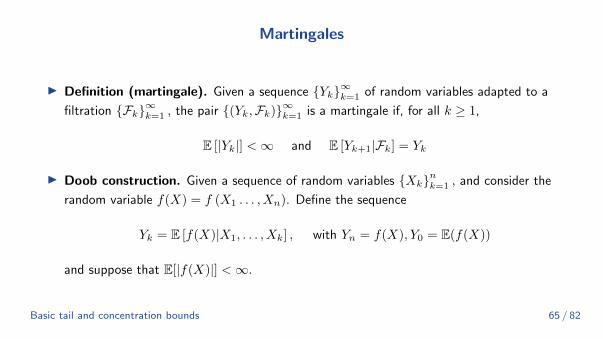
Martingales
I Definition (martingale). Given a sequence {Yk}∞k=1 of random variables adapted to a
filtration {Fk}∞k=1 , the pair {(Yk,Fk)}∞k=1 is a martingale if, for all k ≥ 1,
E [|Yk|] <∞ and E [Yk+1|Fk] = Yk
I Doob construction. Given a sequence of random variables {Xk}nk=1 , and consider the
random variable f(X) = f (X1 . . . , Xn). Define the sequence
Yk = E [f(X)|X1, . . . , Xk] , with Yn = f(X), Y0 = E(f(X))
and suppose that E[|f(X)|] <∞.
Basic tail and concentration bounds 65 / 82
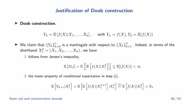
Justification of Doob construction
I Doob construction.
Yk = E [f(X)|X1, . . . , Xk] , with Yn = f(X), Y0 = E(f(X))
I We claim that {Yk}nk=0 is a martingale with respect to {Xk}nk=1 . Indeed, in terms of the
shorthand Xk1 = (X1, X2, . . . , Xk) , we have
1 follows from Jensen’s inequality,
E [|Yk|] = E[∣∣∣E [f(X)|Xk
1
]∣∣∣] ≤ E[|f(X)|] <∞
2 the tower property of conditional expectation in step (i),
E[Yk+1|Xk
1
]= E
[E[f(X)|Xk+1
1
]|Xk
1
](i)= E
[f(X)|Xk
1
]= Yk
Basic tail and concentration bounds 66 / 82
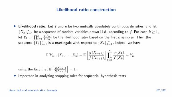
Likelihood ratio construction
I Likelihood ratio. Let f and g be two mutually absolutely continuous densities, and let
{Xk}∞k=1 be a sequence of random variables drawn i.i.d. according to f. For each k ≥ 1,
let Yk :=∏k`=1
g(Xt)f(X`)
be the likelihood ratio based on the first k samples. Then the
sequence {Yk}∞k=1 is a martingale with respect to {Xk}∞k=1 . Indeed, we have
E [Yn+1|X1, . . . , Xn] = E[g (Xn+1)
f (Xn+1)
] n∏k=1
g (Xk)
f (Xk)= Yn
using the fact that E[g(Xn+1)f(Xn+1)
]= 1.
I Important in analyzing stopping rules for sequential hypothesis tests.
Basic tail and concentration bounds 67 / 82

Martingale difference sequence
I Definition (martingale difference sequence). A closely related notion is that of
martingale difference sequence, meaning an adapted sequence {(Dk,Fk)}∞k=1 such that, for
all k ≥ 1,
E [|Dk|] <∞ and E [Dk+1|Fk] = 0
I As suggested by their name, such difference sequences arise in a natural way from
martingales. In particular, given a martingale {(Yk,Fk)}∞k=0 , let us define for k ≥ 1
Dk = Yk − Yk−1
I We then have
E [Dk+1|Fk] = E [Yk+1|Fk]− E [Yk|Fk] = E [Yk+1|Fk]− Yk = 0
Basic tail and concentration bounds 68 / 82

Telescoping decomposition
I Using the martingale property and the fact that Yk is measurable with respect to Fk Thus,
for any martingale sequence {Yk}∞k=0 , we have the telescoping decomposition
f(X)− E(f(X)) = Yn − Y0 =
n∑k=1
(Yk − Yk−1) =
n∑k=1
Dk
where {Dk}∞k=1 is a martingale difference sequence.
I This decomposition plays an important role in our development of concentration
inequalities to follow.
Basic tail and concentration bounds 69 / 82

Concentration bounds for martingale difference sequences
I Theorem (Bernstein-Freedman). Let {(Dk,Fk)}∞k=1 be a martingale difference
sequence, and suppose that E[eλDk |Fk−1
]≤ eλ2v2
k/2 almost surely for any |λ| < 1/αk.
Then the following hold:
(a)∑nk=1Dk ∈ SE
(∑nk=1 v
2k, α∗
)where α∗ := maxk αk. (same as if they were independent)
(b) The sum satisfies the concentration inequality
P
[∣∣∣∣∣n∑k=1
Dk
∣∣∣∣∣ ≥ t]≤
2e− t2
2∑nk=1
v2k if 0 ≤ t ≤
∑nk=1 v
2k
α∗
2e− t
2α∗ if t >∑nk=1 v
2k
α∗
Basic tail and concentration bounds 70 / 82
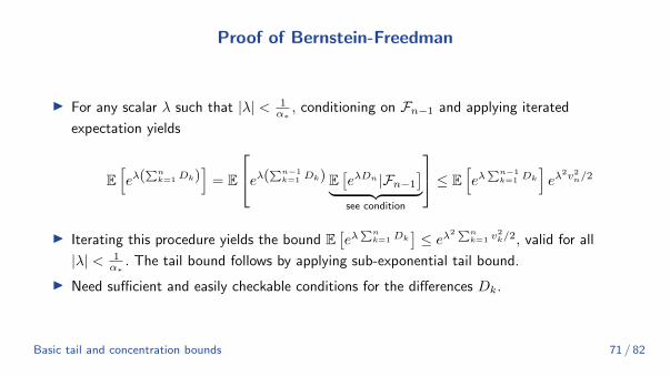
Proof of Bernstein-Freedman
I For any scalar λ such that |λ| < 1α∗, conditioning on Fn−1 and applying iterated
expectation yields
E[eλ(
∑nk=1 Dk)
]= E
eλ(∑n−1k=1 Dk) E
[eλDn |Fn−1
]︸ ︷︷ ︸see condition
≤ E[eλ
∑n−1k=1 Dk
]eλ
2v2n/2
I Iterating this procedure yields the bound E[eλ
∑nk=1 Dk
]≤ eλ2 ∑n
k=1 v2k/2, valid for all
|λ| < 1α∗. The tail bound follows by applying sub-exponential tail bound.
I Need sufficient and easily checkable conditions for the differences Dk.
Basic tail and concentration bounds 71 / 82

Azuma-Hoeffding
I Corollary (Azuma-Hoeffding). Let ({(Dk,Fk)}∞k=1) be a martingale difference sequence
for which there are constants {(ak, bk)}nk=1 such that Dk ∈ [ak, bk] almost surely for all
k = 1, . . . , n. Then, for all t ≥ 0
P
[∣∣∣∣∣n∑k=1
Dk
∣∣∣∣∣ ≥ t]≤ 2e
− 2t2
Σnk−1(bk−ak)2
I Proof Hint.
– Since Dk ∈ [ak, bk] almost surely,
– the conditioned variable (Dk|Fk−1) ∈ [ak, bk] almost surely,
– and hence applying the result of property of sub-Gaussian R.V. (Hoeffding’s lemma).
Basic tail and concentration bounds 72 / 82

Application: bounded difference function
I Given vectors x, x′ ∈ Rn and an index k ∈ {1, 2, . . . , n}, define a new vector x\k ∈ Rn via
x\kj :=
{xj if j 6= k
x′k if j = k
I With this notation, we say that f : Rn → R satisfies the bounded difference inequality with
parameters (L1, . . . , Ln) if, for each index k = 1, 2, . . . , n∣∣∣f(x)− f(x\k)∣∣∣ ≤ Lk for all x, x′ ∈ Rn (2)
I For instance, if the function f is L-Lipschitz with respect to the Hamming norm
dH(x, y) =∑ni=1 I [xi 6= yi] , then the bounded difference inequality holds with parameter
L uniformly across all coordinates. (Recall the definition of L-Lipschitz)
Basic tail and concentration bounds 73 / 82

Bounded difference inequality
I Corollary (Bounded differences inequality). Suppose that f satisfies the bounded
difference property 2 with parameters (L1, . . . , Ln) and that the random vector
X = (X1, X2, . . . , Xn) has independent components. Then
P[|f(X)− E[f(X)]| ≥ t] ≤ 2e− 2t2∑n
k=1L2k for all t ≥ 0
I Recalling the Doob martingale and constructing two corresponding auxiliary R.V.
Dk = E [f(X) | X1, . . . , Xk]− E [f(X) | X1, . . . , Xk−1]
Ak := infx
E [f(X) | X1, . . . , Xk−1, x]− E [f(X) | X1, . . . , Xk−1]
Bk := supx
E [f(X) | X1, . . . , Xk−1, x]− E [f(X) | X1, . . . , Xk−1]
Find something? Dk ≤ Bk −Ak a.s. and recall the definition Bk −Ak ≤ Lk a.s.Basic tail and concentration bounds 74 / 82
Application of Bounded difference inequality
I Example 2.22 (Classical Hoeffding from bounded differences)
I Example 2.23 (U-statistics)
I Example 2.24 (Clique number in random graphs)
I Example 2.25 (Rademacher complexity)
Basic tail and concentration bounds 75 / 82

Outline
Introduction to the seminar series
Why Non-Asymptotic?
Basic tail and concentration bounds
Classical boundsSub-Gaussian
Sub-Exponential
Martingale based methods
Lipschitz functions of Gaussian variables
Basic tail and concentration bounds 76 / 82
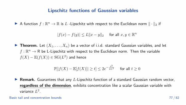
Lipschitz functions of Gaussian variables
I A function f : Rn → R is L -Lipschitz with respect to the Euclidean norm ‖ · ‖2 if
|f(x)− f(y)| ≤ L‖x− y‖2 for all x, y ∈ Rn
I Theorem. Let (X1, . . . , Xn) be a vector of i.i.d. standard Gaussian variables, and let
f : Rn → R be L-Lipschitz with respect to the Euclidean norm. Then the variable
f(X)− E(f(X)) ∈ SG(L2) and hence
P[|f(X)− E[f(X)]| ≥ t] ≤ 2e−t2
2L2 for all t ≥ 0
I Remark. Guarantees that any L-Lipschitz function of a standard Gaussian random vector,
regardless of the dimension, exhibits concentration like a scalar Gaussian variable with
variance L2.
Basic tail and concentration bounds 77 / 82

Proof
I Assume f is also differentiable, we prove a slightly weak version with loose constant.
I Lemma. Suppose that f : Rn → R is differentiable. Then for any convex function
φ : R→ R, we have
E[φ(f(X)− E[f(X)])] ≤ E[φ(π
2〈∇f(X), Y 〉
)]where X,Y ∼ N (0, In) are standard multivariate Gaussian, and independent
Basic tail and concentration bounds 78 / 82

Proof
I Using this lemma with convex fn. φ(x) = exp(λx) for any fixed λ ∈ R,
EX [exp(λ{f(X)− E[f(X)]})] ≤ EX,Y
exp
N (0,λ2π2
4 ‖∇f(X)‖22)︷ ︸︸ ︷(λπ
2〈Y,∇f(X)〉
)| X
= EX
[exp
(λ2π2
8‖∇f(X)‖22
)]using the fact if Z ∼ N (0, σ2), then E(exp(Z)) = exp(σ2/2)
Basic tail and concentration bounds 79 / 82

Proof
I Using this lemma with convex fn. φ(x) = exp(λx) for any fixed λ ∈ R,
EX [exp(λ{f(X)− E[f(X)]})] ≤ EX
exp
λ2π2
8‖∇f(X)‖22︸ ︷︷ ︸≤L2
≤ exp (
1
8λ2π2L2)
I f(X)− E[f(X)] ∈ SG((πL2 )2)
I See proof of the lemma in the book.
Basic tail and concentration bounds 80 / 82
Applications
I Example 2.28 (χ2 concentration )
I Example 2.29 (Order statistics)
I Example 2.30 (Gaussian complexity)
I Example 2.31 (Gaussian chaos variables)
I Example 2.32 (singular values of Gaussian random matrices)
Basic tail and concentration bounds 81 / 82
References I
S. Boucheron, G. Lugosi, and P. Massart. Concentration inequalities: A nonasymptotic theory
of independence. Oxford university press, 2013.
C. Jin, P. Netrapalli, R. Ge, S. M. Kakade, and M. I. Jordan. A short note on concentration
inequalities for random vectors with subgaussian norm. arXiv preprint arXiv:1902.03736, 2019.
M. J. Wainwright. High-dimensional statistics: A non-asymptotic viewpoint, volume 48.
Cambridge University Press, 2019.
Basic tail and concentration bounds 82 / 82