Group Motion Segmentation Using a Spatio-Temporal Driving Force Model

Ruonan Li and Rama ChellappaDepartment of Electrical and Computer Engineering, and Center for Automation Research, UMIACS

University of Maryland, College Park, MD 20742{liruonan,rama}@umiacs.umd.edu

Abstract

We consider the ‘group motion segmentation’ problemand provide a solution for it. The group motion segmenta-tion problem aims at analyzing motion trajectories of mul-tiple objects in video and finding among them the ones in-volved in a ‘group motion pattern’. This problem is moti-vated by and serves as the basis for the ‘multi-object activityrecognition’ problem, which is currently an active researchtopic in event analysis and activity recognition. Specifically,we learn a Spatio-Temporal Driving Force Model to char-acterize a group motion pattern and design an approach forsegmenting the group motion. We illustrate the approachusing videos of American football plays, where we identifythe offensive players, who follow an offensive motion pat-tern, from motions of all players in the field. Experimentsusing GaTech Football Play Dataset validate the effective-ness of the segmentation algorithm.

1. IntroductionIn this work we consider the problem of group motion

segmentation, and propose a solution for it. The group mo-tion segmentation problem arises from video surveillanceapplications and sports video analysis, where a ‘group mo-tion’ involving multiple participants is of interest. Specif-ically, we have in hand point trajectories from consecutiveframes of a video sequence, and aim to group them into twoor more clusters. While this may appear to be similar to thetraditional motion segmentation problems [5, 7, 13, 16, 26,33, 35, 36, 32], it is actually different in the following sense.During group motion, the participating objects/people havedistinctive and varying motions but the group itself collec-tively demonstrates an underlying activity of a particularpattern, while the non-participating group of objects/peopledoes not demonstrate that pattern. A recent developmentin the area of video analysis and activity recognition is theneed for analyzing these motion patterns of the participatinggroup, which are also called ‘multi-object’ or ‘group’ activ-ities [17, 31, 12, 14, 21, 11, 8, 37, 23, 19, 24, 28], and vari-

ous approaches have been proposed to recognize the groupmotion pattern or detect a change or an anomaly. However,these works assume that all objects are involved in the activ-ity, which is far from realistic scenarios where only a por-tion of the objects/people contribute to the specific groupmotion. The group motion segmentation problem exploredhere attempts to divide the point trajectories into partici-pating group and non-participating group, or into multipleparticipating groups, each corresponding to a group activity.

It is important to look into examples of ‘group motion’patterns of interest and see where the challenges are. Onecan think of simple cases where the group of people paradetoward the same direction with same speed [17], or passen-gers getting out of a plane and walking towards the terminalfollow a stationary dynamics [31]. In these cases a devi-ation from the stationary model is detected as an ‘event’or an ‘anomaly’. In more complex problems, a limitednumber of participants interact with each other, and typi-cal activities include approaching, chasing, hand-shaking,robbery, fighting, etc. [12, 21, 11, 37, 23, 24, 28]. Also, agroup activity in an outdoor airport ramp [8] involves sev-eral individual activities occurring in a constrained area andin a specific temporal order. The most challenging caseis American football plays involving a greater number ofparticipants, where the task is to recognize the play strat-egy of the offensive players from their moving trajectories[14, 19]. In a football play, the offensive players are theparticipants of the group motion of offense while the defen-sive players are non-participants. Different offensive partic-ipants will give rise to different moving trajectories, whilethe group will collaboratively demonstrate an ensemble mo-tion pattern which can be identified as a semantic strat-egy represented as a play diagram in the playbook. Thisgroup motion pattern manifests itself as the spatial con-straint and temporal co-occurrence among the interactingtrajectories. Note that participants move under the guidanceof a play diagram but significant spatio-temporal variationsexist among different realizations. Also, the participatingand non-participating group are mixed within the same area,thus non-distinguishable by simply partitioning the spatial

1

Figure 1. Samples from GaTech Football Play Dataset. The toprow gives snapshots of videos of the plays and bottom row con-tains corresponding trajectories. The red trajectories are offensiveones and the blue defensive ones. The trajectories are displayed inground plane coordinates for better visualization.

domain. For these reasons, we address the group motionsegmentation problem in the context of offensive playeridentification in football plays. Examples of the group mo-tion patterns under our consideration are given in Figure 1.Note that our segmentation is based on motion only: wedo not make use of appearance based features, which maynot be always available due to poor video quality or otherreasons.

There are additional challenges beyond the aforemen-tioned ones. Though the participating group of a footballplay consists of a constant number of objects, more gener-ally the group motion pattern may be executed by a vary-ing number of agents in different realizations, and the num-ber may change during the activity due to a participant’sdeparture or the arrival of a new member. Moreover, asthe motion trajectories are generated by a tracking algo-rithm, they are noisy. The trajectories may be incomplete,fragmented or missing due to limitations of the tracking al-gorithm, strong occlusion among objects, and other issuessuch as video quality. Each of these challenges should beaddressed by a vision algorithm and indeed our method isable to handle them.

Turning back to traditional motion segmentation prob-lems we find the majority of them addressing trajecto-ries of feature points from independent 3-D rigid objects[5, 7, 13, 16, 26, 33] and the problem eventually boils downto subspace clustering. Other works also exploit depen-dant/articulated rigid body motion [36] or a motion modelleading to nonlinear manifold clustering [32]. The groupmotion segmentation problem considered here has little incommon with them. On the other hand, the non-rigidStructure-from-Motion problems [4, 3, 34] assume non-rigid shape to be linear combination of rigid ones, and non-rigid motion segmentation [35] makes use of local piece-wise subspace model, while the group motion under ourconsideration does not belong to either of these cases.

In this work we employ Lie group theory [27] and inparticular establish a statistical model over Lie algebra. Lie

group and Lie algebra based approaches play roles in invari-ant visual modeling and recognition [9, 25], robotics [6],3-D rigid motion estimation [10, 1, 30], as well as denseflow field modeling [20]. In this work, we discuss a newapplication to group motion estimation.

The proposed model is detailed in Section 2, and its ap-plication to group motion segmentation is presented in Sec-tions 3 and 4. Section 5 empirically demonstrates the appli-cation of the approach, followed by a discussion in Section6.

2. Spatio-Temporal Driving Force Model for AGroup Motion Pattern

In this section we introduce a characterization for agroup motion pattern, made of a collection of spatio-temporal constrained trajectories possibly noisy, of vary-ing number, and undergoing spatio-temporal variation fromrealization to realization. The key idea is that we modelthe group motion as a dynamic process driven by a spatio-temporal driving force densely distributed across the areawhere the motion occurs, instead of simply as a set of dis-crete point trajectories. To be precise, the driving forceis denoted as a 3 × 3 real matrix 𝐹 (𝑡0, 𝑡𝑓 , 𝑥, 𝑦) whichmoves an object located at 𝑋(𝑡0) = (𝑥(𝑡0), 𝑦(𝑡0), 1)

𝑇 inhomogeneous coordinates at time 𝑡0 to location 𝑋(𝑡𝑓 ) =(𝑥(𝑡𝑓 ), 𝑦(𝑡𝑓 ), 1)

𝑇 at time 𝑡𝑓 , by

𝑋(𝑡𝑓 ) = 𝐹 (𝑡0, 𝑡𝑓 , 𝑥, 𝑦)𝑋(𝑡0). (1)

Without loss of generality, we usually take 𝑡0 = 0 to bethe starting time. It is obvious that once we have learned𝐹 for all 𝑡𝑓 , 𝑥, and 𝑦, then the group motion is completelycharacterized. To be able to learn 𝐹 , we limit our attentionto those parametric 𝐹 ’s which have the following proper-ties: 1) 𝐹 (𝑡1, 𝑡2, 𝑥, 𝑦)𝐹 (𝑡2, 𝑡3, 𝑥, 𝑦) = 𝐹 (𝑡1, 𝑡3, 𝑥, 𝑦); 2)𝐹 (𝑡1, 𝑡2, 𝑥, 𝑦)

−1 = 𝐹 (𝑡2, 𝑡1, 𝑥, 𝑦); and 3)

𝐹 (𝑡, 𝑡+ 1, 𝑥, 𝑦) ≜ 𝐹 (𝑡, 𝑥, 𝑦) =⎡⎣ 𝐹11(𝑡, 𝑥, 𝑦) 𝐹12(𝑡, 𝑥, 𝑦) 𝐹13(𝑡, 𝑥, 𝑦)𝐹21(𝑡, 𝑥, 𝑦) 𝐹22(𝑡, 𝑥, 𝑦) 𝐹23(𝑡, 𝑥, 𝑦)

0 0 1

⎤⎦ .(2)

The 𝐹 (𝑡, 𝑥, 𝑦)’s defined this way is in fact a Lie group andmore specifically an affine group [27]. By making use ofLie group theory we may achieve both generality and flexi-bility in modeling complex motion patterns, as shown next.

𝐹 (𝑡, 𝑥, 𝑦) characterizes the motion potential at time 𝑡 foran object located at (𝑥, 𝑦). However, we may look into analternative representation. Consider 𝐹 (𝑡, 𝑡 + 𝛿𝑡, 𝑥, 𝑦) and𝑋(𝑡 + 𝛿𝑡) = 𝐹 (𝑡, 𝑡 + 𝛿𝑡, 𝑥, 𝑦)𝑋(𝑡), and we then have𝑋(𝑡 + 𝛿𝑡) − 𝑋(𝑡) = (𝐹 (𝑡, 𝑡 + 𝛿𝑡, 𝑥, 𝑦) − 𝐼)𝑋(𝑡) where𝐼 is the identity matrix. Dividing both sides by 𝛿𝑡 andletting 𝛿𝑡 → 0, we get 𝑋 ′(𝑡) = f(𝑡, 𝑥, 𝑦)𝑋(𝑡), in which

𝑋 ′(𝑡) = (𝑥′(𝑡), 𝑦′(𝑡), 0)𝑇 is the speed of the object, and

f(𝑡, 𝑥, 𝑦) =

⎡⎣ 𝑓11(𝑡, 𝑥, 𝑦) 𝑓12(𝑡, 𝑥, 𝑦) 𝑓13(𝑡, 𝑥, 𝑦)𝑓21(𝑡, 𝑥, 𝑦) 𝑓22(𝑡, 𝑥, 𝑦) 𝑓23(𝑡, 𝑥, 𝑦)

0 0 0

⎤⎦ ≜

lim𝛿𝑡→0

⎡⎣ 𝐹11(𝑡,𝑡+𝛿𝑡,𝑥,𝑦)−1𝛿𝑡

𝐹12(𝑡,𝑡+𝛿𝑡,𝑥,𝑦)𝛿𝑡

𝐹13(𝑡,𝑡+𝛿𝑡,𝑥,𝑦)𝛿𝑡

𝐹21(𝑡,𝑡+𝛿𝑡,𝑥,𝑦)𝛿𝑡

𝐹22(𝑡,𝑡+𝛿𝑡,𝑥,𝑦)−1𝛿𝑡

𝐹23(𝑡,𝑡+𝛿𝑡,𝑥,𝑦)𝛿𝑡

0 0 0

⎤⎦ .

(3)In fact, f(𝑡, 𝑥, 𝑦) is the Lie algebraic representation of𝐹 (𝑡, 𝑥, 𝑦) and the two are related by the exponentialmap 𝐹 (𝑡, 𝑥, 𝑦) = exp(f(𝑡, 𝑥, 𝑦)) =

∑∞𝑖=0

1𝑖! f(𝑡, 𝑥, 𝑦)

𝑖

and logarithmic map f(𝑡, 𝑥, 𝑦) = log(𝐹 (𝑡, 𝑥, 𝑦)) =∑∞𝑖=1

(−1)𝑖−1

𝑖 (𝐹 (𝑡, 𝑥, 𝑦)−𝐼)𝑖 [27]. In other words, we maywork equivalently with f instead of directly working with 𝐹for the driving force model. The advantage of using f liesin the fact that the space of all f ’s, the Lie algebra, is a lin-ear one on which we may develop various statistical tools,while the Lie group of 𝐹 ’s is a nonlinear manifold not easyto work with. More importantly, 𝑋 ′(𝑡) = f(𝑡, 𝑥, 𝑦)𝑋(𝑡)implies that the location and speed of the object are linearlyrelated by f , and both the location and the speed are low-level features obtainable from the motion trajectories of theobjects, i.e., learning a single driving force model f(𝑡, 𝑥, 𝑦)will be straightforward.

2.1. Learning a Spatial Hybrid Driving Force Modelat a Time Instant

Suppose we fix a specific time instant 𝑡. Intuitively,different driving forces f(𝑡, 𝑥, 𝑦)’s induce different ‘affine’motions for different (𝑥, 𝑦)’s, and learning for all (𝑥, 𝑦)’sin the whole area of group motion is intractable. On theother hand, constant f(𝑡, 𝑥, 𝑦) ≡ f(𝑡) induces a global‘affine’ motion to all objects in the group, whose represen-tative power is severely limited. For this reason, we pro-pose a spatial hybrid model, in which we assume 𝐾 drivingforces in the area of group motion. The effective area ofthe 𝑘th (𝑘 = 1, 2, ⋅ ⋅ ⋅ ,𝐾) force is Gaussian distributed as(𝑥, 𝑦)𝑇 ∼ 𝒩 (𝜇𝑘,Σ𝑘). (We drop the argument 𝑡 in thissubsection for simplicity.) In the effective area, there is auniform ‘affine’ motion f𝑘. For notational convenience wewrite

f𝑘 =

[𝐴𝑘 b𝑘

0𝑇 0

](4)

where 𝐴𝑘 is the upper-left 2× 2 block of f𝑘.Consider the feature vector 𝑌 ≜ (𝑥, 𝑦, 𝑥′, 𝑦′)𝑇 extracted

from an object motion trajectory driven by the 𝑘th force,and it is obvious that

𝑌 =

[𝐼𝐴𝑘

] [𝑥𝑦

]+

[0b𝑘

]. (5)

Taking into account the noise created due to approximat-ing the speed (1st order derivative) of point trajectories, we

represent the observed feature vector as

y = 𝑌 +

[0n𝑘

](6)

where n ∼ 𝒩 (0, 𝑇 𝑘). Then after some manipulations wefind y ∼ 𝒩 (𝜈𝑘,Γ𝑘), where

𝜈𝑘 =

[𝜇𝑘

𝐴𝑘𝜇𝑘 + b𝑘

](7)

and

Γ𝑘 =

[Σ𝑘 Σ𝑘𝐴𝑘𝑇

𝐴𝑘Σ𝑘 𝐴𝑘Σ𝑘𝐴𝑘𝑇 + 𝑇 𝑘

]. (8)

We are now in a position to learn the spatial hybrid driv-ing force model for a particular time instant 𝑡, from a limiteddiscrete number of objects in a group motion. Suppose wehave observed 𝑡𝑀 motion feature vectors {y𝑚}𝑡𝑀𝑚=1, thenthe learning task boils down to fitting a Gaussian MixtureModel (GMM) of 𝐾 component {(𝜈𝑘,Γ𝑘)}𝐾𝑘=1 (using uni-form mixing coefficient 1

𝐾 ). An Expectation-Maximizationprocedure is employed to complete the inference. Aftersuccessfully learning the GMM, the spatial hybrid drivingmodel, i.e., {(f𝑘, 𝜇𝑘,Σ𝑘)}𝐾𝑘=1, is recovered. Note that byGaussian assumption the learned effective areas of differentdriving force components will overlap and cover the wholearea; to eliminate this ambiguity we technically partition thearea such that the distance between the component’s centerand (𝑥, 𝑦) is minimized.

It may be useful to recap what has been achieved till nowby using the spatial hybrid driving force model. In fact, attime 𝑡 we partition the area into 𝐾 subareas, and model theinstant motions of all the objects in one subarea to be anuniform ‘affine’ motion. In this way we are actually es-tablishing a dense ‘motion potential field’ across the areawhere the group motion happens. Though the field maybe learned from motion features of sparse objects, it existseverywhere, and any other group of objects giving rise tothe same field model is regarded as the same group motionpattern at time 𝑡, though participating objects (which themotion features come from) may appear in different loca-tions from one group pattern to another. Figure 2 gives twoexamples of the spatial hybrid driving force model, wherethe sparse objects for learning the model, the learned parti-tion of the area, as well as the learned driving force in eachpartition are all shown for two group motion samples in thedataset.

2.2. Learning Temporal Evolution of Driving ForceModels for a Group Motion Pattern

Having obtained a hybrid driving force model at a par-ticular time instant, we turn to the temporal evolution of themodel, which eventually characterizes the complete groupmotion. Denote the driving force model at time 𝑡 as 𝔐(𝑡) =

Figure 2. Two samples of 3-component driving force model at atime instant. The red circles denote the relative objects (offensiveplayers) and the red bars attached to them denote the velocitiesof the objects. The blue arrow array gives the densely distributeddriving force learned from the sparse object motion observations.The contour lines enclose the effective areas for the driving forces.

{m𝑘(𝑡)}𝐾𝑘=1 where m𝑘(𝑡) = (f𝑘(𝑡), 𝜇𝑘(𝑡),Σ𝑘(𝑡)), and as-sume we have learned models at time 𝑡 = 𝑡1, 𝑡2, ⋅ ⋅ ⋅ , 𝑡𝑇(which may not be continuous, but intermittent instants dueto fragmented trajectories). We then learn a temporal se-quence of these models in two steps: 1) component align-ment between two consecutive instants, and 2) learning aparametric representation for the temporal sequence.

Component alignment is performed on 𝔐(𝑡𝑖+1) withrespect to aligned 𝔐(𝑡𝑖), starting from 𝔐(𝑡2) withrespect to 𝔐(𝑡1). Mathematically, let the vector(𝑘1, 𝑘2, ⋅ ⋅ ⋅ , 𝑘𝐾)𝑇 denote the element-wise permutation ofvector (1, 2, ⋅ ⋅ ⋅ ,𝐾)𝑇 , then we aim to find an optimal per-mutation such that

∑𝐾𝑗=1 𝐷(m𝑗(𝑡𝑖),m

𝑘𝑗 (𝑡𝑖+1)) is mini-mized, where 𝐷(m,m′) is a properly defined dissimilar-ity between model m and m′. In other words, we are try-ing to associate each driving force component at time 𝑡𝑖+1

uniquely with one at time 𝑡𝑖 such that within each associ-ated pair are they as similar as possible. We then give eachcomponent at 𝑡𝑖+1 a new component index which is nothingbut that of the associated component at 𝑡𝑖. Obviously, aftercomponent alignment for a fixed 𝑘, m𝑘(𝑡) become similar,or change smoothly, among all 𝑡𝑖’s, which reduces the com-plexity of the parametric representation.

Note that the driving force model m includes the ‘force’term f and the effective area 𝒩 (𝜇,Σ), and f lies on the Liealgebra which is a linear space. Therefore, we use

𝐷(m,m′) = ∥f − f ′∥+𝛼(𝐾𝐿(𝒩 (𝜇,Σ)∥𝒩 (𝜇′,Σ′)) +𝐾𝐿(𝒩 (𝜇′,Σ′)∥𝒩 (𝜇,Σ)))

(9)where 𝐾𝐿(⋅∥⋅) denotes the Kullback-Leibler divergence.Then the optimal permutation can be solved using the clas-sical Hungarian assignment algorithm [18].

Now we are looking for a parametric representation of

11

221

2

Figure 3. A pictorial illustration of the temporal evolution of driv-ing force models. It only shows the 𝑘th component. In all, thereshould be 𝐾 ones, i.e., on left and right planes there should be 𝐾straight lines respectively.

the temporal sequence 𝔐(𝑡) for 𝑡 = 1, 2, ⋅ ⋅ ⋅ . Note thatm𝑘(𝑡) is essentially composed of f𝑘(𝑡) , the space of whichis a Lie algebra (denoted as 𝔉), and 𝒩 (𝜇𝑘(𝑡),Σ𝑘(𝑡)),which is on the nonlinear manifold of 2 × 2 Gaus-sian’s. As the nonlinearity brings analytical difficulty,we work with the parameters of 𝒩 (𝜇𝑘(𝑡),Σ𝑘(𝑡)), i.e.,[𝜇𝑘

1(𝑡), 𝜇𝑘2(𝑡), 𝜎

𝑘11(𝑡), 𝜎

𝑘12(𝑡)(= 𝜎𝑘

21(𝑡)), 𝜎𝑘22(𝑡)]

𝑇 ≜ g𝑘(𝑡),rather than the Gaussian itself, and regard the space ofg𝑘(𝑡)’s (denoted as 𝔊) to be linear as well. (Though lin-earity does not rigorously hold, it is an effective approxi-mation.)

We hence establish a parametric model for the tempo-ral sequence 𝔐(𝑡), 𝑡 = 1, 2, ⋅ ⋅ ⋅ on the Cartesian productspace 𝔉×𝔊. We propose the linear model {(W𝑘𝑡+w𝑘 +v1,U

𝑘𝑡+ u𝑘 + v2)}𝐾𝑘=1 for {(f𝑘(𝑡),g𝑘(𝑡))}𝐾𝑘=1, where

W𝑘 =

⎡⎣ 𝑊 𝑘11 𝑊 𝑘

12 𝑊 𝑘13

𝑊 𝑘21 𝑊 𝑘

22 𝑊 𝑘23

0 0 0

⎤⎦ , (10)

U𝑘 = [𝑈𝑘1 , 𝑈

𝑘2 , 𝑈

𝑘3 , 𝑈

𝑘4 , 𝑈

𝑘5 ]

𝑇 , and v1,v2 are independentwhite Gaussian perturbation. With this model, f𝑘(𝑡)’s (resp.g𝑘(𝑡)’s) for each component 𝑘, when 𝑡 varies, will approx-imately move in the one-dimensional subspace of 𝔉 (resp.𝔊). In other words, components of the time-varying spa-tial hybrid driving force will evolve along straight lines in𝔉×𝔊. A visual illustration for this idea is shown in Figure3.

We use linear representations for the temporal sequenceof driving forces basically for simplicity and effectiveness(to be demonstrated in the experiment). We may attempt ad-vanced techniques but in this initial work on group motionsegmentation we use linear ones to begin with. The straightlines {(W𝑘𝑡 + w𝑘,U𝑘𝑡 + u𝑘)}𝐾𝑘=1 in 𝔉 × 𝔊 are simplyfitted using previously obtained models (f𝑘(𝑡),g𝑘(𝑡))’s attime 𝑡 = 𝑡1, 𝑡2, ⋅ ⋅ ⋅ , 𝑡𝑇 in the least square sense. However,once these lines are available, we may re-sample the linesat other 𝑡’s to generate new spatial hybrid driving forces atthose time instants. In this way, we actually learn the groupmotion pattern within the whole time duration from onlymotion information at limited time instants.

Up to now, a group motion pattern has been fully cap-tured by {(W𝑘𝑡 +w𝑘,U𝑘𝑡 + u𝑘)}𝐾𝑘=1 ≜ 𝐺𝑀 , by whichthe motions of participants of the group activity, at any loca-tion and any time, are condensed into and may be recoveredfrom the corresponding 𝐺𝑀 .

3. DP-DFM: Accounting for Group MotionVariation

The variation of group motion patterns from video tovideo leads to the variation of 𝐺𝑀 ’s learned from videoto video. To statistically model this variability among dif-ferent 𝐺𝑀 ’s, we establish a Dirichlet Process (DP) [2] over𝔉×𝔊, leading to a Dirichlet Process - Driving Force Model(DP-DFM). The DP-DFM is essentially a Bayesian mixturemodel good for handling an unknown number of mixingcomponents. As we do not have prior knowledge about thevariability of the group motion patterns (i.e., 𝐺𝑀 ’s fromdifferent offensive plays), DP-DFM is a natural choice.

Specifically, we regard the 𝐺𝑀 as a long vector con-sisting of the elements of W𝑘,w𝑘,U𝑘,u𝑘, 𝑘 = 1, ⋅ ⋅ ⋅ ,𝐾,and suppose it comes in the following manner (called ‘StickBreaking’): 1) Let 𝑣𝑡 ∼ 𝐵𝑒𝑡𝑎(1, 𝜂) and 𝜆𝑡 = 𝑣𝑡Π

𝑡−1𝑙=1(1 −

𝑣𝑙); 2) Draw a sample from Σ∞𝑡=1𝜆𝑡𝛿(𝜃𝑡), where 𝛿(𝜃𝑡) is a

point measure situated at parameter vector 𝜃𝑡, and 𝜃𝑡 ∼ 𝒢0,which is a base measure (Gaussian-Wishart in this work); 3)Draw a 𝐺𝑀 from a Gaussian whose mean and covarianceare specified by 𝜃𝑡. In this way the DP-DFM formulationhas become a canonical DP mixture problem and we em-ploy the standard procedure [2] to complete the inferenceof DP-DFM.

4. Probabilistic SegmentationWith a DP-DFM learned from training group motion pat-

terns, we perform segmentation on a new testing motionpattern by synthesizing a set of Monte Carlo samples (i.e.,spatio-temporal DFM’s) from DP-DFM, matching the tra-jectories in the testing motion pattern with these simulatedmodels, and voting for the best matched motion trajecto-ries as the segmentation result. To simulate a Monte Carlosample, we first draw a 𝐺𝑀 from the DP-DFM. Then werecover the temporal sequence of spatially hybrid drivingforces 𝔐(𝑡) = {m𝑘(𝑡)}𝐾𝑘=1, and consequently the time-varying densely distributed driving forces 𝐹 (𝑡, 𝑥, 𝑦). As aresult, at each time instant 𝑡 and for each object(trajectory)at 𝑡 in the testing motion pattern, we may predict its loca-tion at 𝑡 + 1 by (1), and measure the discrepancy betweenthe predicted and actual locations (The discrepancy is sim-ply measured as the distance between the two in this work).Those objects(trajectories) which accumulatively have theleast discrepancies across all 𝑡’s with all simulated drivingforce samples are finally determined as the participating ob-jects.

5. Experiments5.1. GaTech Football Play Dataset

We perform group motion segmentation on the GaT-ech Football Play Dataset, dividing players into participat-ing (offensive) ones and non-participating (defensive) onessolely by their motion trajectories. The GaTech FootballPlay Dataset is a newly established dataset for group mo-tion pattern/activity modeling and analysis. Recent worksusing this dataset [19, 29] reported results on play strat-egy recognition. The dataset consists of a collection of 155NCAA football game videos (of which 56 are now avail-able). Each video is a temporally segmented recording ofan offensive play, i.e., the play starts at the beginning of thevideo and terminates at the end. Accompanied with eachvideo is a ground-truth annotation of the object locations ineach frame. The annotation includes coordinates in the im-age plane of all the 22 players as well as field landmarks- the intersections of the field lines. Using the landmarkinformation we can compute the plane homographies andconvert motion coordinates into ground plane trajectories.We show the ground truth trajectories (in the ground planecoordinates) of sample plays in Figure 1.

We perform three rounds of experiments, the first ofwhich employs ground-truth trajectories from training totesting. As in any practical system the input trajectories willbe noisy, in the second round we generate noisy trajectoriesfrom the ground-truth and experiment with them. In thefinal round we test the learned framework on tracks com-puted from videos with a state-of-art multi-object tracker.In each round of experiments, we carry out multiple passesof five-fold evaluations, i.e., in each pass we randomly di-vide 4/5 of the samples into the training set and the remain-ing samples into testing set. The final statistics is aggre-gated from the average of all passes. Empirically we find𝐾 = 5 is a good selection for the total number of compo-nents. For Gaussian-Wishart prior 𝒢0, we set the Wishartscale matrix to be the inverse of sample covariance of train-ing 𝐺𝑀 ’s, and Gaussian mean to be the sample mean oftraining 𝐺𝑀 ’s. The other free parameters in the frameworkare determined by experimental evaluation.

5.2. Experiment on Ground­Truth TrajectoriesIn the experiment with ground-truth trajectories, we have

approximately 56× 4/5 group motion samples, which maybe captured in different views. For convenience and with-out loss of generality, we apply a homographic transformto each of them to work in a canonical view (ground planein this work). To get sufficient exemplars to train the DP-DFM, we augment the training sets by generating new train-ing samples from the original ones. For this purpose, weperturb each original trajectory by adding 2-D isotropicGaussian on ground-plane coordinates at multiples of 20%of the whole motion duration, and polynomially interpolat-

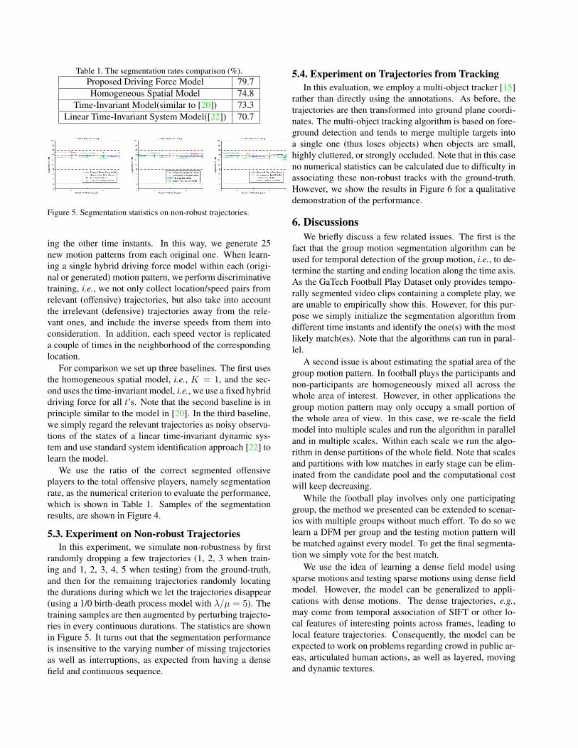
Table 1. The segmentation rates comparison (%).Proposed Driving Force Model 79.7Homogeneous Spatial Model 74.8

Time-Invariant Model(similar to [20]) 73.3Linear Time-Invariant System Model([22]) 70.7

Figure 5. Segmentation statistics on non-robust trajectories.

ing the other time instants. In this way, we generate 25new motion patterns from each original one. When learn-ing a single hybrid driving force model within each (origi-nal or generated) motion pattern, we perform discriminativetraining, i.e., we not only collect location/speed pairs fromrelevant (offensive) trajectories, but also take into accountthe irrelevant (defensive) trajectories away from the rele-vant ones, and include the inverse speeds from them intoconsideration. In addition, each speed vector is replicateda couple of times in the neighborhood of the correspondinglocation.

For comparison we set up three baselines. The first usesthe homogeneous spatial model, i.e., 𝐾 = 1, and the sec-ond uses the time-invariant model, i.e., we use a fixed hybriddriving force for all 𝑡’s. Note that the second baseline is inprinciple similar to the model in [20]. In the third baseline,we simply regard the relevant trajectories as noisy observa-tions of the states of a linear time-invariant dynamic sys-tem and use standard system identification approach [22] tolearn the model.

We use the ratio of the correct segmented offensiveplayers to the total offensive players, namely segmentationrate, as the numerical criterion to evaluate the performance,which is shown in Table 1. Samples of the segmentationresults, are shown in Figure 4.

5.3. Experiment on Non­robust TrajectoriesIn this experiment, we simulate non-robustness by first

randomly dropping a few trajectories (1, 2, 3 when train-ing and 1, 2, 3, 4, 5 when testing) from the ground-truth,and then for the remaining trajectories randomly locatingthe durations during which we let the trajectories disappear(using a 1/0 birth-death process model with 𝜆/𝜇 = 5). Thetraining samples are then augmented by perturbing trajecto-ries in every continuous durations. The statistics are shownin Figure 5. It turns out that the segmentation performanceis insensitive to the varying number of missing trajectoriesas well as interruptions, as expected from having a densefield and continuous sequence.

5.4. Experiment on Trajectories from TrackingIn this evaluation, we employ a multi-object tracker [15]

rather than directly using the annotations. As before, thetrajectories are then transformed into ground plane coordi-nates. The multi-object tracking algorithm is based on fore-ground detection and tends to merge multiple targets intoa single one (thus loses objects) when objects are small,highly cluttered, or strongly occluded. Note that in this caseno numerical statistics can be calculated due to difficulty inassociating these non-robust tracks with the ground-truth.However, we show the results in Figure 6 for a qualitativedemonstration of the performance.

6. DiscussionsWe briefly discuss a few related issues. The first is the

fact that the group motion segmentation algorithm can beused for temporal detection of the group motion, i.e., to de-termine the starting and ending location along the time axis.As the GaTech Football Play Dataset only provides tempo-rally segmented video clips containing a complete play, weare unable to empirically show this. However, for this pur-pose we simply initialize the segmentation algorithm fromdifferent time instants and identify the one(s) with the mostlikely match(es). Note that the algorithms can run in paral-lel.

A second issue is about estimating the spatial area of thegroup motion pattern. In football plays the participants andnon-participants are homogeneously mixed all across thewhole area of interest. However, in other applications thegroup motion pattern may only occupy a small portion ofthe whole area of view. In this case, we re-scale the fieldmodel into multiple scales and run the algorithm in paralleland in multiple scales. Within each scale we run the algo-rithm in dense partitions of the whole field. Note that scalesand partitions with low matches in early stage can be elim-inated from the candidate pool and the computational costwill keep decreasing.

While the football play involves only one participatinggroup, the method we presented can be extended to scenar-ios with multiple groups without much effort. To do so welearn a DFM per group and the testing motion pattern willbe matched against every model. To get the final segmenta-tion we simply vote for the best match.

We use the idea of learning a dense field model usingsparse motions and testing sparse motions using dense fieldmodel. However, the model can be generalized to appli-cations with dense motions. The dense trajectories, e.g.,may come from temporal association of SIFT or other lo-cal features of interesting points across frames, leading tolocal feature trajectories. Consequently, the model can beexpected to work on problems regarding crowd in public ar-eas, articulated human actions, as well as layered, movingand dynamic textures.

(a) Ground truth (b) Proposed DFM (c) Homogeneous Spatial

model

(d) Time-invariant model

(similar to [21])

(e) Linear time-invariant

system ([23])

Figure 4. Samples of segmentation results. In each row are a ground-truth group motion and corresponding segmentation results. Redtrajectories denote the relevant objects and blue ones are irrelevant ones.

(a) Ground truth (b) Proposed DFM (c) Homogeneous Spatial

model

(d) Time-invariant model

(similar to [21])

(e) Linear time-invariant

system ([23])

Figure 6. Samples of segmentation results on trajectories from tracking. In each row are a ground-truth group motion and correspondingsegmentation results on tracks. Red trajectories denote the relevant objects and blue ones are irrelevant ones.

The model is not view-invariant. We need to learn aseparate model for each static view. However, static cam-eras are typical for surveillance and also commonly usedfor sports recordings. Also, the synthesis and voting basedmethod is not computationally economic, and thus needsfurther improvement.

A final point is that though we designed methods in the

context of group motion segmentation, the learned model,or compact features derived from it, can potentially serveas representatives of the underlying group motion. This im-plies a possibility that the proposed framework can be usedtoward the original motivating application - group activityrecognition. Meanwhile, it is also expected that integrationof the model into a multi-object tracker will help to improve

the tracking quality due to its capability to predict potentialmotion. These open issues are under our further investiga-tion.

Acknowledgement: The authors thank Sima Taheri, Dr.Shaohua Kevin Zhou, and Minhua Chen for assistances anddiscussions. The authors also thank GaTech Athletic As-sociation and GaTech School of Interactive Computing forproviding the dataset. This work was funded by the VIRATprogram.

References[1] E. Bayro-Corrochano and J. Ortegon-Aguilar. Lie alge-

bra approach for tracking and 3d motion estimation usingmonocular vision. Image and Vision Computing, 25:907 –921, 2007. 2

[2] D. Blei and M. Jordan. Variational inference for dirichletprocess mixtures. Journal of Bayesian Analysis, 1:121 – 144,2006. 5

[3] M. Brand. Morphable 3d models from video. In CVPR,2001. 2

[4] C. Bregler, A. Hertzmann, and H. Biermann. Recoveringnon-rigid 3d shape from image streams. In CVPR, 2000. 2

[5] J. Costeira and T. Kande. A multibody factorization methodfor independently moving objects. International Journal ofComputer Vision, 29:159 – 179, 1998. 1, 2

[6] T. Drummond and R. Cipolla. Application of lie algebras tovisual servoing. International Journal of Computer Vision,37:21 – 41, 2000. 2

[7] C. Gear. Multibody grouping from motion images. Interna-tional Journal of Computer Vision, (29):133 – 150, 1998. 1,2

[8] S. Gong and T. Xiang. Recognition of group activities usingdynamic probabilistic networks. In ICCV, 2003. 1

[9] L. V. Gool, T. Moons, E. Pauwels, and A. Oosterlinck. Visionand lies approach to invariance. Image and Vision Comput-ing, 13:259 – 277, 1995. 2

[10] V. M. Govindu. Lie-algebraic averaging for globally consis-tent motion estimation. In CVPR, 2004. 2

[11] A. Hakeem and M. Shah. Learning, detection and represen-tation of multi-agent events in videos. Artificial Intelligence,171:586 – 605, 2007. 1

[12] S. Hongeng and R. Nevatia. Multi-agent event recognition.In ICCV, 2001. 1

[13] N. Ichimura. Motion segmentation based on factorizationmethod and discriminant criterion. In ICCV, 1999. 1, 2

[14] S. Intille and A. Bobick. Recognizing planned, multipersonaction. Computer Vision and Image Understanding, 81:414– 445, 2001. 1

[15] S. Joo and R. Chellappa. A multiple-hypothesis approachfor multiobject visual tracking. IEEE Transactions on ImageProcessing, 16(11):2849 – 2854, 2007. 6

[16] K. Kanatani. Motion segmentation by subspace separationand model selection. In ICCV, 2001. 1, 2

[17] S. M. Khan and M. Shah. Detecting group activities usingrigidity of formation. In ACM Multimedia 2005, November2005. 1

[18] H. W. Kuhn. The hungarian method for the assignment prob-lem. Naval Research Logistics Quarterly, (2):83 – 97, 1955.4

[19] R. Li, R. Chellappa, and S. Zhou. Learning multi-modaldensities on discriminative temporal interaction manifold forgroup activity recognition. In CVPR, 2009. 1, 5

[20] D. Lin, E. Grimson, and J. Fisher. Learning visual flows: Alie algebraic approach. In CVPR, 2009. 2, 6

[21] X. Liu and C. Chua. Multi-agent activity recognition usingobservation decomposedhidden markov models. Image andVision Computing, 24(2):166 – 175, February 2006. 1

[22] L. Ljung. System Identification - Theory for the User. Pren-tice Hall, 1999. 6

[23] X. Ma, F. Bashir, A. Khokhar, and D. Schonfeld. Event anal-ysis based on multiple interactive motion trajectories. IEEETransactions on Circuits and Systems for Video Technology,19:397 – 406, 2009. 1

[24] B. Ni, S. Yan, and A. Kassim. Recognizing human groupactivities by localized causalities. In CVPR, 2009. 1

[25] R. P. N. Rao and D. L. Ruderman. Learning lie groups forinvariant visual perception. In NIPS, 1999. 2

[26] S. R. Rao, R. Tron, R. Vidal, and Y. Ma. Motion segmenta-tion via robust subspace separation in the presence of outly-ing, incomplete, or corrupted trajectories. In CVPR, 2008. 1,2

[27] W. Rossmann. Lie Groups: An Introduction through LinearGroups. Oxford University Press, 2003. 2, 3

[28] M. S. Ryoo and J. K. Aggarwal. Spatio-temporal relation-ship match: Video structure comparison for recognition ofcomplex human activities. In ICCV, 2009. 1

[29] E. Swears and A. Hoogs. Learning and recognizing Amer-ican football plays. In Snowbird Learning Workshop, 2009.5

[30] O. Tuzel, R. Subbarao, and P. Meer. Simultaneous multiple3d motion estimation via mode finding on lie groups. InICCV, 2005. 2

[31] N. Vaswani, A. Roy-Chowdhury, and R. Chellappa. Shapeactivity: A continuous-state hmm for moving/deformingshapes with application to abnormal activity detection. IEEETransactions on Image Processing, 14:1603 – 1616, October2005. 1

[32] R. Vidal and Y. Ma. A unified algebraic approach to 2-d and3-d motion segmentation. Journal of Mathematical Imagingand Vision, 25:403 – 421, 2006. 1, 2

[33] R. Vidal, Y. Ma, and S. Sastry. Generalized principal compo-nent analysis (GPCA). IEEE Transactions on Pattern Anal-ysis and Machine Intelligence, 27:1945 – 1959, 2005. 1, 2

[34] J. Xiao, J. Chai, and T. Kanade. A closed-form solution tonon-rigid shape and motion recovery. In ECCV, 2004. 2

[35] J. Yan and M. Pollefeys. A general framework for motionsegmentation: Independent, articulated, rigid, non-rigid, de-generate and non-degenerate. In ECCV, 2006. 1, 2

[36] L. Zelnik-Manor and M. Irani. Degeneracies, dependenciesand their implications in multi-body and multi-sequence fac-torizations. In CVPR, 2003. 1, 2

[37] Y. Zhou, S. Yan, and T. S. Huang. Pair-activity classificationby bi-trajectories analysis. In CVPR, 2008. 1