GROUND STATE OF 10Li AND 13Be

By

Shigeru Kennedy Yokoyama

A DISSERTATION

Submitted toMichigan State University

in partial fulfillment of the requirementsfor the degree of

DOCTOR OF PHILOSOPHY

Department of Physics and Astronomy

1996

ABSTRACT

GROUND STATE OF 10Li AND 12Be

By

Shigeru Kennedy Yokoyama

11Li nucleus is known to have the structure of a 9Li core and a two-neutron halo and is the

heaviest particle stable Li isotope. The ground state study of 10Li is important to understand

the structure of 11Li since it has information on the n +9Li interaction which determines a

significant part of the 11Li three body structure. A direct mass measurement of 10Li is im-

possible since it has very short lifetime (~10-21 s). Previous experimental studies have

shown conflicting results for the 10Li ground state. 13Be information is also crucial for un-

derstanding of 14Be structure similar to the 10Li and 11Li case. The goal of the current work

is to determine the ground state properties of 10Li and 13Be.

The technique of sequential neutron decay spectroscopy (SNDS) was employed around

0˚ for the present study. The nuclei 10Li, and 13Be were created via fragmentation. They

decayed immediately in the target and emitted a neutron and a fragment (9Li and 12Be)

which were separated with magnets and detected. The relative velocity spectra were created

from the experimental information. Monte Carlo simulations were performed and the re-

sults were compared with the data. The limit of the decay constants for each isotope were

extracted via χ2 analysis.

The low-lying s-wave ground state was established for 10Li at Er ≈ 50 keV or as ≈ -40

fm. The result of 13Be could be either interpreted as a low-lying s-wave state or the tail of

the known state at 2.0 MeV.

iii

To my wife, Kelly

iv

ACKNOWLEDGMENTS

First, I would like to thank my advisor, Michael Thoennessen. He has always been a

great help to me. His perspective always helped me stay on the right track and showed me

the way to proceed. I could never have come this far without his help.

I thank professors Pawel Danielewicz, Michael Harrison, Wayne Repko, and Brad

Sherrill for being my guidance committee. I also thank professor Gregers Hansen for in-

sightful discussions and providing the scattering length calculations. As a collaborator, I re-

ally enjoyed having discussions with professor Aaron Galonsky.

I learned a lot from a former post-doc of our research group, Robert A. Kryger. He es-

pecially contributed to the improvement of my computer skills a great deal. Peter Thirolf,

a former post-doc, was a good example to me in his way of being unintimidated with having

too many things to do. His solid way of handling complicated tasks influenced my attitude

toward the thesis writing.

It was very lucky for me to be able to work with Easwar Ramakrishnan, Afshin Azhari,

Thomas Baumann, and Marcus Chromik as colleagues. I believe we were one of the best

‘teams’ in the NSCL. I would like to thank Afshin Azhari and Mike Fauerbach for their

proofreading of my thesis drafts.

It was really enjoyable interacting with the people in the NSCL including John ‘Ned’

Kelley, Raman Pfaff, Don Sackett, Larry Phair, Mike Lisa, Wen-Chen Hsi, Tong Li, Eu-

v

gene Gualtieri, Stefan Hannuschke, Q. Pan, Damian Handzy, Jim Brown, Magie Hellström,

Chris Powell, Jon Kruse, Jing Wang, Phil Zecher, Mathias Steiner, Sally Gaff, Barry

Davids, Heiko Scheit, Thomas Glasmacher, Jac Caggiano, Njema Frazier, Corn Williams,

Richard Ibbotson, Roy Lemmon, Gerd Kunde, Razvan Popescu, Luke Chen, Renan Fontus,

and Kyoko Fuchi.

I would like to thank all the staff of the NSCL, especially Raman Anantaraman, Reg

Ronningen, Richard Au, Ron Fox, Barbara Pollack, John Yurkon, Dennis Swan, Dave

Sanderson, and Craig Snow. They saved me from many troubles I encountered while I con-

ducted experiments and research in the NSCL.

My experience at the NSCL gave me the privilege to meet international visitors such as

Toshiyuki Kubo, Yoshiyuki Iwata, and Ákos Horváth. Meeting and working with people

from all over the world was a very unique and valuable experience.

I also would like to thank my computer at home PowerMacintosh 7500/100, Zip drive,

and 28.8kbps modem for their stable operation. I wrote the thesis with this system. At the

beginning of 1996, 100MHz clock speed and 28.8kbps modem was kind of fast but I’m sure

that readers will find it ridiculously slow in the very near future.

I would like to thank my friend Dr. Frederick I. Kaplan for his encouragement and help

in my life in Michigan.

I am also thankful for my friendship family in Michigan, Roy and Elaine Pentilla. Their

hospitality was very heart warming especially during the cold holiday season in Michigan.

I thank my family in Japan and my brother Naohiko in L.A. for all sorts of support. I’m

glad that all of my family could visit me in East Lansing while I was studying at Michigan

State University.

vi

Finally I thank my wife Kelly Yokoyama Kennedy for her love and support. In finally

reaching this goal I deeply thank all those people around me in Michigan. I will never forget

the people and the beautiful campus of Michigan State University.

1

Chapter 1

Introduction

The field of exotic nuclei is currently one of the most active areas studied in nuclear phys-

ics. Recent advancements of equipment and facilities have provided unique opportunities

to study nuclei near and beyond the neutron and proton drip lines. There are two major mo-

tivations to study exotic nuclei. One reason to study exotic nuclei is for nuclear astrophys-

ics. The stellar evolution process begins with H and He atoms from the big bang [Rol88].

Starting out with hydrogen burning, the more complex atoms were formed via various nu-

clear reaction cycles such as the CNO (carbon-nitrogen-oxygen) cycle [Won90]. Exotic nu-

clei often play an important role within these reaction cycles and the information on those

nuclei is crucial to explain the abundance of the elements and to determine the age of stars.

Another motivation to study exotic nuclei is that unique tests of the fundamental laws of

physics and nuclear models can be carried out by studying the properties of those nuclei.

Exotic nuclei are either neutron or proton rich. The current work is a study of 10Li and

13Be, which are light nuclei on the neutron dripline. The nuclei 11Li and 9Li are known to

be bound nuclei and 11Li is the heaviest particle stable Li isotope. The nucleus 11Li is also

known to consist of a two-neutron halo around a 9Li core. Unlike other nuclei which have

an uniform nuclear matter density, halo nuclei have a lower nuclear matter density region

(halo) around the normal nuclear matter density region (core). The recent experimental ef-

2

forts to study the halo nuclei also stimulated the interest of theorists. Various model calcu-

lations for the halo nuclei have been reported. For the 11Li case, structure information of

10Li, which is an unbound nucleus, turns out to be crucial for the theoretical calculations as

a subsystem of the halo nucleus 11Li. One of the goals of the current experiment was to

measure the ground state energy level of 10Li. Since it is particle unbound, it is impossible

to measure the energy in a direct way. We employed the technique of neutron sequential

decay spectroscopy at 0˚ and extracted the ground state energy and width of 10Li.

The situation in Be isotopes is similar to the Li isotopes. The nucleus 14Be is the heavi-

est stable isotope and also considered a two-neutron halo nucleus whereas 13Be is particle

unstable. Again the n-12Be interaction, or 13Be is important for the understanding of 14Be.

Previous work and the relations of the 10Li structure to the 11Li model as well as 13Be and

14Be are discussed in the next chapter.

3

Chapter 2

Neutron Halo Nuclei

2.1 The Two-Neutron Halo Nucleus 11Li

11Li is the heaviest particle-stable nucleus among the Li isotopes. It has been known as a

neutron drip-line nucleus since 10Li is unbound toward one neutron decay and 12Li is not

bound either. 11Li has a half-life of 8.2 ms for β- decay to 11Be. Tanihata et al. [Tan85]

measured the interaction cross sections (σI) of lithium isotopes (6Li, 7Li, 8Li, 9Li, and 11Li)

and beryllium isotopes (7Be, 9Be, and 10Be) on the targets of Be, C, and Al at 790 MeV/

nucleon using the novel technique of exotic isotope beams produced through projectile

fragmentation in high energy heavy ion reactions. The extracted root mean square (rms) nu-

clear radii from the σI showed that 11Li has an unusually large radius (RI = 3.14 fm) com-

pared to neighboring nuclei (RI ≈ 1.2 fm x A1/3 [Kra88] (= 2.5 fm for 9Li)). It was

interpreted as a large deformation and/or a long tail in the matter distribution due to the

weakly bound neutrons.

To investigate the nature of the large matter radius of 11Li, different experiments were

performed, for example momentum distribution measurements. Previous studies showed

that the momentum distribution of fragmentation products have a Gaussian distribution

which is isotropic in the projectile rest frame [Gre75]. The width of the Gaussian

4

distribution σ is related to the Fermi momentum or the temperature corresponding to the

nuclear binding energy [Gol74] and the momentum distribution inside the projectile

[Hüf81]. Goldhaber [Gol74] parameterized the width σ of the Gaussian shape momentum

distribution by a single parameter σ0 (reduced width) defined as

(3.1)

where F is the mass number of the fragment and A is the mass number of the projectile.

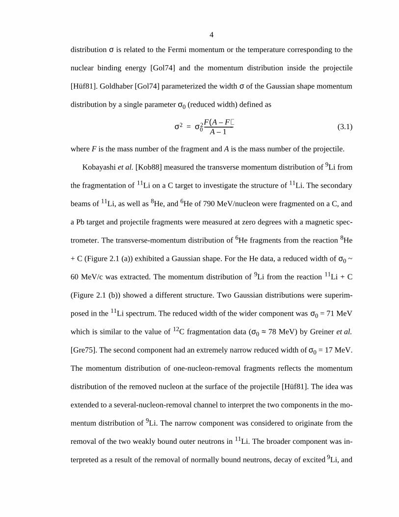
Kobayashi et al. [Kob88] measured the transverse momentum distribution of 9Li from

the fragmentation of 11Li on a C target to investigate the structure of 11Li. The secondary

beams of 11Li, as well as 8He, and 6He of 790 MeV/nucleon were fragmented on a C, and

a Pb target and projectile fragments were measured at zero degrees with a magnetic spec-

trometer. The transverse-momentum distribution of 6He fragments from the reaction 8He

+ C (Figure 2.1 (a)) exhibited a Gaussian shape. For the He data, a reduced width of σ0 ~

60 MeV/c was extracted. The momentum distribution of 9Li from the reaction 11Li + C

(Figure 2.1 (b)) showed a different structure. Two Gaussian distributions were superim-

posed in the 11Li spectrum. The reduced width of the wider component was σ0 = 71 MeV

which is similar to the value of 12C fragmentation data (σ0 ≈ 78 MeV) by Greiner et al.

[Gre75]. The second component had an extremely narrow reduced width of σ0 = 17 MeV.

The momentum distribution of one-nucleon-removal fragments reflects the momentum

distribution of the removed nucleon at the surface of the projectile [Hüf81]. The idea was

extended to a several-nucleon-removal channel to interpret the two components in the mo-

mentum distribution of 9Li. The narrow component was considered to originate from the

removal of the two weakly bound outer neutrons in 11Li. The broader component was in-

terpreted as a result of the removal of normally bound neutrons, decay of excited 9Li, and

σ2 σ02F A F–( )

A 1–----------------------=

5

Figure 2.1: [Kob88] (a) Transverse-momentum distributions of 6He fragments fromthe reaction 8He + C. The solid lines are fitted Gaussian distributions with a reduced widthof σ0 = 59 MeV/c. (b) Transverse-momentum distributions of 9Li fragments from reaction11Li + C. The solid lines are fitted distributions with two Gaussian components. The dottedline is a contribution of the wide component in the 9Li distribution. The reduced width ofthe two components are σ0 = 71 MeV/c and σ0 = 17 MeV/c, respectively.

0

50

0 100 200-100-200

0

50

0 100 200-100-200

P⊥ [MeV/c]

6

the decay of 10Li.

A large root mean square radius, small momentum distribution width component in the

projectile fragmentation, and a small separation energy of the two outer neutrons (Sn =

295keV [You93]), suggest the existence of a large two-neutron halo around the 9Li core in

11Li. This structural characteristic has subsequently been found in many other light neu-

tron-rich nuclei (6He, 11Li, 11Be, 14Be, etc.) [Han95, Tho96].

Before the experimental discovery of the neutron halo, Migdal [Mig73] suggested that

the force between two neutrons may lead to a bound state of the two neutrons and a nucleus

even if a combination of the two do not form a bound state. Hansen and Jonson [Han87]

interpreted Migdal’s suggestion on 11Li as a quasi-deuteron consisting of a 9Li core cou-

pled to a dineutron [2n]. A radial square well potential was assumed for the 9Li core and the

binding energy of the dineutron was assumed to be zero. The external wave function of the

dineutrons outside the core was approximated for the small binding energy B between the

9Li core and the dineutron by

(3.2)

where R is the radius of a square well potential, r is the distance between the 9Li and the

dineutron. The decay length ρ in Equation 3.2 is defined as ρ = h/(2µB)1/2 where µ is the

reduced mass of the system and B is the binding energy. This simple model agrees well

with the experimental results for the radius and the 2n separation energy (see Figure 2.2).

2.2 10Li And 11Li Three-Body Models

After Hansen and Jonson’s two-body calculation [Han87] for 11Li, a number of three-body

model calculations were performed to obtain a more detailed understanding of 11Li. For the

r( ) 2πρ( ) 1 2/– r ρ⁄–[ ]expr

---------------------------R ρ⁄[ ]exp

1 R ρ⁄+( )1 2⁄---------------------------------=

7

Figure 2.2: [Han87] The calculated relations between the matter r.m.s. radius and 2nseparation energy with mass parameters corresponding to 11Li and 6He by Hansen and Jon-son. The experimental values for radii and 2n separation energies were taken from [Tan85]and [Wap85].

8

three-body calculations of 11Li, detailed information about the 10Li states are essential

input parameters.

Bertsch and Esbensen treated 11Li as a three-body system consisting of two interacting

neutrons together with a structureless 9Li core [Ber91]. They used a two-particle Green’s

function technique to describe the two-neutron wave function. A Woods-Saxon potential,

with a kinetic energy operator and a spin-orbit interaction were used for the single particle

Hamiltonian. The numerical test was performed assuming the ground state of 10Li to be a

p1/2 state (see Figure 2.3). The result was compared with the available experimental data

of the 10Li ground state energy at 0.8 MeV [Wil75] and they obtained a two-neutron sepa-

ration energy of 0.20 MeV which is approximately consistent with the available experimen-

tal value of 0.25 ± 0.01 MeV [Thi75, Wou88] at that time.

Bang and Thompson [Ban92] performed three-body calculations for 11Li by applying

Figure 2.3: [Ber91] The dependence of the 11Li two neutron separation energy to the10Li 1p1/2 state energy predicted by Bertsch and Esbensen. The solid line and dashed lineshow correlated and uncorrelated neutron cases, respectively.

9

the Faddeev three body equations [Lav73] using the super soft core potential SSCC

[Tou75], or the Reid soft-core potential RSC [Rei68] for the neutron-neutron potential Vnn.

Choosing parameters to give a 1p3/2 level at the energy of the 9Li neutron separation energy

(-4.1 MeV) and varying 1p1/2 resonance energy between 0.4 and 0.7 MeV, a Woods-Saxon

potential and a spin-orbit term, or a Woods-Saxon potential and a pairing term were used

for the core-neutron potential Vcn. Although they reproduced the main features of the halo

in their results, some inconsistencies were found for fitting both the energies and the radius

of 11Li simultaneously.

Thompson and Zhukov [Tho94] performed a second Faddeev three-body calculation

for 11Li. It was shown that the presence of a near-threshold s-wave virtual state in the 9Li

+ n two-body potential within the three-body calculation for 11Li had an explicit effect on

the calculated structure of the 11Li halo. A Woods-Saxon potential was considered for the

neutron-9Li potential where the s- and p-wave strengths Vs and Vp along with the spin-orbit

strength VSO were varied to fit a particular 2s scattering length while maintaining the 1p1/

2 resonance energy between +0.15 and +0.50 MeV. The 1p3/2 energy was kept constant at

-4.1 MeV which is the neutron separation energy of 9Li. Assuming a nearly 50% s-wave

motion between the halo neutrons and the core, their results agreed very well with the ex-

perimental data obtained by Kobayashi et al. [Kob88] and Orr et al. [Orr92], see Figure 2.4.

The interaction of the halo neutrons was accounted for by using the realistic super-soft-core

nn potential (SSC). Figure 2.5 shows the results of this calculation and it will be compared

with the experimental results presented in Chapter 5.

At the time of these calculations, the only available experimental data of the 10Li

ground state were the measurements by Wilcox et al. [Wil75] and Amelin et al. [Ame90].

10

Figure 2.4: [Tho94] The comparison of the calculated 9Li core momentum distribu-tions from 11Li fragmentation by Thompson and Zhukov and the experimental data by Orret al. (square) and Kobayashi et al. (star). The calculation includes s-wave potential as wellas p-wave potential in n-9Li interaction.

11

Figure 2.5: [Tho94] The calculated relation between 11Li binding energy, p1/2 reso-nance energy, and s1/2 scattering length. The horizontal solid line shows the observedtwo-neutron binding energy of 11Li by Kobayashi et al. [Kob92].

12

Wilcox and collaborators studied 10Li using the 9Be(9Be,8B)10Li reaction with a 121 MeV

9Be beam on a 0.68 mg/cm2 9Be foil. The ground state was observed at Sn = -0.80 ± 0.25

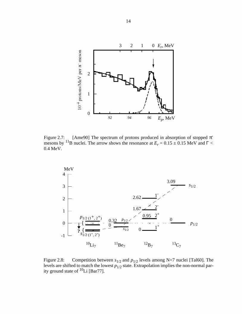
MeV with a width of Γ = 1.2 ± 0.3 MeV (see Figure 2.6). Amelin et al. used the absorption

of stopped π- mesons by 11B nuclei and observed the energy spectrum of protons near the

kinematic limits of the reaction to study 10Li. The resonance parameters of Er = 0.15 ± 0.15

MeV with a width of Γ0 < 0.4 MeV were extracted assuming an s-wave state by fitting the

Breit-Wigner resonance shape using the test, see Figure 2.7.

2.3 Recent Reports of The 10Li Ground State

Shortly after the first measurement of 10Li by Wilcox, Barker and Hickey [Bar77]

discussed the ground state configuration of 10Li. The 10Li structure was compared to the

11Be configuration since both nuclei contain the same number of neutrons. The ground

state of 11Be is known to have a non-normal parity state (J = 1/2+) and is considered to

have 1s41p62s structure. The lowest normal parity state (J = 1/2-) is at 0.32 MeV above

the ground state which is considered to have a 1s41p7 configuration. Since the energy of the

lowest non-normal parity state relative to the lowest normal parity state increases as Z

increases for the nuclei with N = 7 and Z > 4 (1.67 MeV for 12B and 3.09 MeV for 13C)

[Tal60] (Figure 2.8), the ground state of 10Li was expected to have non-normal parity state

(J = 1- or 2-) by extrapolation. A ground state level of the 10Li was estimated using the

available experimental data [Che70] of an T = 2 isobaric analog state of 10Be. The result

showed that it was expected close to 9Li + n threshold and lower than the experimental data

of the 10Li state at 0.8 MeV by Wilcox et al. which was attributed to the lowest normal

parity state.

χ2

13

Figure 2.6: [Wil75] The energy spectra of 8B was obtained from the following reac-tions using 121 MeV 12C beam. (a) 12C(9Be,8B)13B is for an energy calibration, (b)9Be(9Be,8B)10Li is from singles events, and (c) 9Be(9Be,8B)10Li is from coincidenceevents with 9Li from the breakup of the recoiling 10Li. The angle was at 14˚ in the labora-tory.

14

Figure 2.7: [Ame90] The spectrum of protons produced in absorption of stopped π-

mesons by 11B nuclei. The arrow shows the resonance at Er = 0.15 ± 0.15 MeV and Γ <0.4 MeV.

0

1

2

3 2 1 0 Er, MeV

Ep, MeV92 94 96

Figure 2.8: Competition between s1/2 and p1/2 levels among N=7 nuclei [Tal60]. Thelevels are shifted to match the lowest p1/2 state. Extrapolation implies the non-normal par-ity ground state of 10Li [Bar77].

MeV4

3

2

1

0

-1

3.09

0

2.62

1.67

0.95

000.32

s1/2

p1/2

1-

2-

2+

1+{{

p1/2 (1+, 2+) p1/2

s1/2 (1-, 2-)

s1/2?

10Li711Be7

12B713C7

15

The more recent experimental data reported by Bohlen et al. (Figure 2.9) [Boh93] and

Young et al. (Figure 2.10) [You94] established the existence of a p-wave state around 500

keV in 10Li. Bohlen and collaborators [Boh93] used two different transfer reactions,

9Be(13C,12N)10Li at ELab = 336 MeV and 13C(14C,17F)10Li at ELab = 337 MeV, to study

the states of 10Li and concluded that Er = 0.42 ± 0.05 MeV, Γ = 0.15 ± 0.07 MeV is the 1+

ground state and Er = 0.80 ± 0.06 MeV, Γ = 0.30 ± 0.10 MeV is the 2+ first excited state.

Young and collaborators [You94] observed a p-wave state at Er = 0.54 ± 0.06 MeV, Γ =

0.36 ± 0.02 MeV using the reaction 11B(7Li,8B)10Li at ELab = 130 MeV. Evidence for a

low-lying state in 10Li was also seen at Er > 0.100 MeV and Γ < 0.23 MeV.

Kryger et al. [Kry93] employed the method of sequential neutron decay spectroscopy

(SNDS) at 0˚ and observed a central peak in the relative velocity spectrum of 9Li + n

coincidence events which indicates an existence of a low decay energy process (see Figure

Figure 2.10: [You94] The energy spectrum from the transfer reaction 11B(7Li,8B)10Liby Young et al. It shows a strong evidence of the state at Er ≈ 500 keV.

16

Figure 2.9: [Boh93] Energy spectra of 12N from the reaction of 9Be(13C,12N)10Li byBohlen et al. The ground state (Er = 0.42 MeV) and the first excited state at Ex = 0.38 MeV(Er = 0.80 MeV) are not completely resolved.

17

2.11). 10Li was created via fragmentation of an 80 MeV/nucleon 18O beam on a 10 mg/cm2

C target. The fragmentation products and the primary beam were separated from the

neutrons using a set of quadrupole magnets and a dipole magnet. The fragments and the

neutrons were detected in coincidence. Since this method is only sensitive to the Q-value

of the decay, the central peak in the spectrum could represent a decay from an excited state

of 10Li to an excited state of 9Li, as well as a decay from the ground state of 10Li to the

ground state of 9Li. Thus, this observation does not prove the existence of a low-lying

s-wave state, however a limit on the decay parameters for each l (= 0 or 1) could be

extracted assuming the central peak to originate from the decay to a 9Li ground state. The

results reported by Kryger et al. [Kry93] for the p-wave case were Er < 200 keV for a width

Γ0 less than 500 keV and Er < 300 keV for the width Γ0 more than 500 keV and less than

1500 keV. For the s-wave case, Er < 300 keV for the width Γ0 less than 500 keV and Er <

450 keV for the width more than 500 keV and less than 1500 keV.

Zinser et al. [Zin95] used one nucleon stripping reactions of 11Be and 11Li to investi-

gate the states of 10Li. The secondary beams of 280 MeV/nucleon for 11Li and 460 MeV

for 11Be on a 1.29 g/cm2 carbon target were used for the reaction. The fragments were de-

tected after a separation with a magnetic spectrometer. Neutrons were detected in coinci-

dence with the fragments. The neutron data from the events 11Be + C → AZ + n + X and

11Li + C → 9Li + n + X were selected and recorded as a distribution of the radial momentum

pr. Figure 2.12 shows the results of this experiment. As a first order approximation, the one

proton stripping from the 10Be core of the one neutron halo nucleus 11Be most likely did

not disturb the initial state of the s-wave halo neutron and it became an unbound neutron in

10Li. Thus it was suggested that the 10Li state seen by Kryger et al. and the narrow momen-

18

Figure 2.11: [Kry93] The relative velocity spectra of 9Li + n coincidence events ob-tained with sequential neutron decay spectroscopy by Kryger et al. The dashed line is asimulated spectrum with the parameter by Wilcox et al. (Er = 800 keV, l = 1) superimposedon the Gaussian background (dotted). The solid line is a simulated spectrum with the pa-rameter by Amelin et al. (Er = 150 keV, l = 0) plus the Gaussian background.

19

Figure 2.12: [Zin95] Radial momentum distributions of neutrons from 10Li breakup re-ported by Zinser et al. 10Li was created by one proton stripping from 11Be (top) or by oneneutron stripping from 11Li (bottom). In the top figure, the top dotted line assumes an l =1 resonance at 0.05 MeV. The two sets (as = -5 and -50 fm) of the calculations were shownwith the 9Li recoil widths Q = 100 MeV/c (solid) and Q = 0 MeV/c. In the bottom figure,two contributions were considered in the theoretical curves. One is diffraction (1/3 inten-sity) and the other is the intermediate state of 10Li (2/3 intensity) which was assumed tobe a pure s state.

20

tum distribution in the results were attributed to the s-wave neutrons in 10Li. Also, one neu-

tron stripping from the 11Li beam, to create 10Li, could be considered not to affect the 9Li

core because of the weak binding between the halo neutron and the core. Thus it was very

unlikely to excite the 9Li core to the 2.7 MeV first excited state and the observed state must

have been due to the ground state of 10Li. The parameter Γ of a two-dimensional Lorentzian

was used to parameterize the distribution, and the results from both 11Be and 11Li beams

showed the same Γ = 36 MeV/c. The Woods-Saxon single-particle potential-well model

was used for the fit and the depth of the p well was fixed to reproduce a resonance at 0.42

MeV [Boh93].

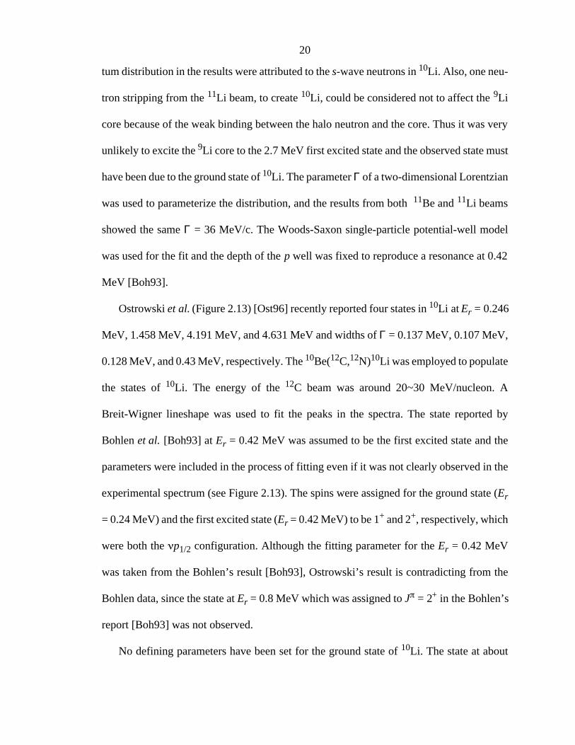
Ostrowski et al. (Figure 2.13) [Ost96] recently reported four states in 10Li at Er = 0.246

MeV, 1.458 MeV, 4.191 MeV, and 4.631 MeV and widths of Γ = 0.137 MeV, 0.107 MeV,

0.128 MeV, and 0.43 MeV, respectively. The 10Be(12C,12N)10Li was employed to populate

the states of 10Li. The energy of the 12C beam was around 20~30 MeV/nucleon. A

Breit-Wigner lineshape was used to fit the peaks in the spectra. The state reported by

Bohlen et al. [Boh93] at Er = 0.42 MeV was assumed to be the first excited state and the

parameters were included in the process of fitting even if it was not clearly observed in the

experimental spectrum (see Figure 2.13). The spins were assigned for the ground state (Er

= 0.24 MeV) and the first excited state (Er = 0.42 MeV) to be 1+ and 2+, respectively, which

were both the p1/2 configuration. Although the fitting parameter for the Er = 0.42 MeV

was taken from the Bohlen’s result [Boh93], Ostrowski’s result is contradicting from the

Bohlen data, since the state at Er = 0.8 MeV which was assigned to J = 2+ in the Bohlen’s

report [Boh93] was not observed.

No defining parameters have been set for the ground state of 10Li. The state at about

21

Figure 2.13: [Ost96] Spectra of the 10Be(12C,12N)10Li reaction by Ostrowski et al. Al-though the state reported by Bohlen et al. [Boh93] at Er = 0.42 MeV was assumed to bethere for fitting, it is not resolved from the ground state at Er = 0.24 MeV. The state report-ed by Wilcox et al. at 0.8 MeV was not observed in these spectra.

22

0.50 MeV with a p-wave emission reported by Bohlen et al. [Boh93] and Young et al.

[You94] are at least in agreement, however the energies and/or angular momentum

assignments of the lower-lying state are still controversial.

2.4 14Be Three-Body Models and 13Be Ground State

Similar to 11Li, a 14Be nucleus is considered to have a two neutron halo structure which

consists of a 12Be core and two weakly bound halo neutrons [Tho96]. The ground state of

13Be has the same importance to the theoretical models of 14Be as the structure of 10Li does

to the 11Li three-body calculations [Tho96].

Ostrowski et al. [Ost92] performed an experiment to study 13Be using the

double-charge-exchange reaction 13C(14C,14O)13Be, ELab = 337.3 MeV. A highly enriched

(98%) 13C target as well as a 12C target were used in the (14C,14O)-reaction. The 12C target

was used to calibrate and to determine the background. The states observed were at 2.01

MeV, 5.14 MeV, 8.53 MeV above 12Be + n and Γ = 0.3 MeV, 0.4 MeV, 0.9 MeV,

respectively. R-matrix calculations of the line width suggested the probable spin state for

the lowest observed state to be J = 5/2+ or 1/2-. A theoretical calculation by Poppelier et

al. [Pop85] using the (0+1)hω shell-model, and a prediction by Lenske [Len91] using a

Woods-Saxon potential with a density dependent pairing interaction, supported the J = 5/

2+ assignment for the state at 2.01 MeV. Although the latter calculation also predicted a

low-lying 1/2+ ground state at around 0.9 MeV, it was not observed in this experiment. It

was argued that the ground state was not observed in the spectrum, because of the low cross

section of the 2s1/2 neutron-shell in multi-nucleon transfer reaction and the large s-state

level width.

23

Penionzhkevich [Pen94] reported states in 13Be using the 14C(11B,12N)13Be reaction.

A new state at 0.9 MeV was observed as well as the previously reported state at 2.0 MeV.

However, this ground state has not yet been confirmed by other experiments.

Korsheninnikov [Kor95] used a secondary beam of 12Be from an 18O primary beam on

a 5 mg/cm2 thick CD2 target to study the states in 13Be populated via the neutron transfer

reaction d(12Be,p). Figure 2.14 shows the results obtained in this experiment which exhib-

its clear evidence for the known 2 MeV state as well as states at 5 MeV, 7 MeV, and 10

MeV above the neutron decay threshold. However, background due to the carbon in the tar-

get (dotted line in the figure) did not allow for a reliable measurement in the low-energy

region of the spectrum.

Descouvemont [Des94] performed a 12Be + n microscopic cluster model calculation

Figure 2.14: [Kor95] The proton spectrum from the reactions CD2(12Be,p) (solid) andC(12Be,p) (dotted). The lowest state extracted reliably is at Er = 2 MeV.

24

for 13Be. The Volkov force [Vol65] V2 and V4 were used for the nuclear part of the nucle-

on-nucleon interaction. The result of the calculations showed the existence of a slightly

bound low-lying 1/2+ state at E = -9 keV for V2 and at E = -38 keV for V4, which are both

lower than the 5/2+ state (E = 2.01 MeV) reported by Ostrowski et al [Ost92]. It suggests

that the inversion of d5/2+ and s1/2+ occurs.

As in the 11Li [Tho94] case, Thompson and Zhukov [Tho96] performed similar

three-body calculations of 14Be. While the simple shell model predicts a (1d5/2)2

configuration for the ground state of 14Be, an admixture of (s1/2)2 and (d5/2)2

configurations were assumed and the neutron-core interaction potentials for both s1/2 and

d5/2 was considered. First, it was shown that a d-wave state at 2.1 MeV on 13Be alone did

not lead to the bound 14Be nucleus which contradicted the experimental result (bound by

1.34 MeV [Aud93]). Among several combinations of the 2s and 1d neutron resonances,

only a combination of a 2s virtual state with a large scattering length (as ≈ -130 fm) and

another d-wave state at E ≈ 1.3 MeV which was lower than the known 2.1 MeV d-wave

state, reproduced the experimental values of the two neutron binding energy and the matter

radius of the 14Be, simultaneously. More experimental results are awaited to confirm the

low-lying structure of the 13Be as an important step in the 14Be three-body calculation.

25

Chapter 3

Experimental Details

3.1 Experimental Method

The primary goal of the present work was to determine the ground state energy of 10Li. The

technique of sequential neutron decay spectroscopy [Deá87] (SNDS) was employed to

fragmentation products produced near 0˚. Figure 3.1 shows a kinematic diagram of the 10Li

→ 9Li + n decay. If a 10Li nucleus is produced by fragmentation, it initially has a non-zero

V

Vnlab

Vfraglab

VnCM

VfragCM

Center of Mass

neutron

9Li

10Li

Figure 3.1: Kinematic diagram of the sequential neutron spectroscopy for the 10Li de-cay.

Vrel

26

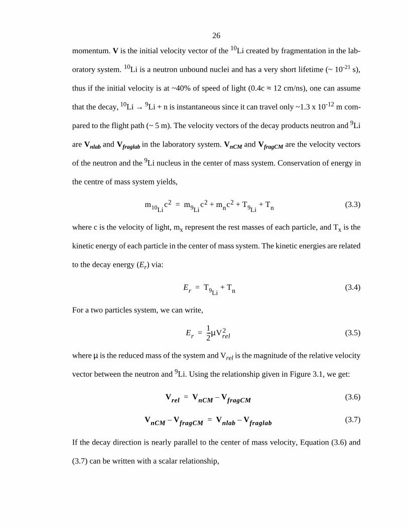
momentum. V is the initial velocity vector of the 10Li created by fragmentation in the lab-

oratory system. 10Li is a neutron unbound nuclei and has a very short lifetime (~ 10-21 s),

thus if the initial velocity is at ~40% of speed of light (0.4c ≈ 12 cm/ns), one can assume

that the decay, 10Li → 9Li + n is instantaneous since it can travel only ~1.3 x 10-12 m com-

pared to the flight path (~ 5 m). The velocity vectors of the decay products neutron and 9Li

are Vnlab and Vfraglab in the laboratory system. VnCM and VfragCM are the velocity vectors

of the neutron and the 9Li nucleus in the center of mass system. Conservation of energy in

the centre of mass system yields,

(3.3)

where c is the velocity of light, mx represent the rest masses of each particle, and Tx is the

kinetic energy of each particle in the center of mass system. The kinetic energies are related

to the decay energy (Er) via:

(3.4)

For a two particles system, we can write,

(3.5)

where µ is the reduced mass of the system and Vrel is the magnitude of the relative velocity

vector between the neutron and 9Li. Using the relationship given in Figure 3.1, we get:

(3.6)

(3.7)

If the decay direction is nearly parallel to the center of mass velocity, Equation (3.6) and

(3.7) can be written with a scalar relationship,

mLi10 c2 m

Li9 c2 mnc2 TLi9 Tn+ + +=

Er TLi9 Tn+=

Er12---µVrel

2=

Vrel VnCM VfragCM–=

VnCM VfragCM– Vnlab Vfraglab–=

27

(3.8)

where Vnlab and Vfraglab are the magnitude of the corresponding vectors.

During the actual data analysis, the relative velocity spectrum was obtained from the

velocity information of the 9Li and the neutrons. This information was then compared to

Monte Carlo simulations to extract the mass of 10Li.

3.2 Mechanical Setup

The experiment was performed at the National Superconducting Cyclotron Laboratory

(NSCL). Figure 3.2 shows a floor plan of the NSCL. An 18O beam with a kinetic energy of

80 MeV / nucleon was provided from the K1200 cyclotron. The primary beam bombarded

a 94 mg / cm2 thick 9Be target located in front of the last quadrupole-dipole magnet

combination in the beam transport system of the NSCL. Fragmentation in the target created

various nuclei. Table 3.1 shows a example of a prediction of fragmentation products by the

code INTENSITY [Win92] for the present case. Since the INTENSITY calculation does

not include unbound nuclei, 10Li is not included in Table 3.1. Figure 3.3 shows the

schematic of the experimental setup. The 10Li nuclei break up immediately after their

creation in the target into one neutron and a 9Li fragment. The dipole magnet was used to

bend the primary beam and the fragments, respectively, away from the straight flight path

of the neutrons into two properly adjusted separate beamlines. The first one at 11˚ was for

the fragments and had a telescope detector array at the end. The primary beam then bent

into the 14˚ beamline and was collected in a shielded Faraday cup at a distance of ~ 25 m

to reduce the background. The neutrons from the breakup were detected by a liquid

scintillator array located ~ 5.8 m down stream at 0˚. The neutrons were extremely forward

Vrel Vnlab Vfraglab–=

28

29

Table 3.1: A example of an output file of the INTENSITY [Win92] calculation for an

80 MeV/nucleon 18O beam (intensity = 10 pnA) with a 94 mg/cm2 9Be Target.

Fragment B-rho Energy Rate(charge) [Tm] [MeV/A] [#/s]

3He(2+) 1.8448 70.320 34494He(2+) 2.4620 70.441 107346He(2+) 3.6962 70.561 43688He(2+) 4.9305 70.621 426Li(3+) 2.4587 70.260 261917Li(3+) 2.8701 70.337 279338Li(3+) 3.2816 70.396 118929Li(3+) 3.6930 70.441 214711Li(3+) 4.6118 73.424 77Be(4+) 2.1468 69.973 184319Be(4+) 2.7640 70.158 6346310Be(4+) 3.1089 71.833 3310811Be(4+) 3.4534 73.201 781012Be(4+) 3.7976 74.340 89114Be(4+) 4.4856 76.127 28B (5+) 1.9583 69.664 394010B (5+) 2.4813 71.510 10356611B (5+) 2.7570 72.912 14739812B (5+) 3.0326 74.079 9588413B (5+) 3.3079 75.064 3055014B (5+) 3.5831 75.908 513715B (5+) 3.8582 76.638 4959C (6+) 1.8315 69.340 25410C (6+) 2.0618 71.112 553011C (6+) 2.2917 72.556 4880912C (6+) 2.5214 73.756 18597813C (6+) 2.7510 74.770 32691614C (6+) 2.9804 75.637 28478915C (6+) 3.2097 76.388 13305016C (6+) 3.4389 77.043 3518517C (6+) 3.6681 77.622 37212N (7+) 2.1554 73.373 650113N (7+) 2.3522 74.420 6478114N (7+) 2.5490 75.315 30034715N (7+) 2.7456 76.090 69889116N (7+) 2.9421 76.767 89771517N (7+) 3.1386 77.363 69214318N (7+) 3.3350 77.892 1589919N (7+) 3.5314 78.365 120

30

31

focused due to the high primary beam energy. 9Li fragments were detected in coincidence

with the neutrons at the end of beam pipe bent by 11˚ with respect to the central neutron

fright path. The fragment flight path distance from the target to the fragment telescope was

~ 6.0 m. The quadrupole magnets and the dipole magnet were tuned to optimize the

detection rate of 9Li and other charged nuclei with a mass-to-charge ratio equal to three

(6He, 12Be, 15B).

The detector system and the signal processing electronics are described in the following

sections.

3.3 Neutron Detectors

Five liquid scintillator (NE213) detectors were used to detect the neutrons. Each neutron

detector had a cylindrical shape, and Figure 3.4 (a) shows their dimensions. Figure 3.4 (b)

shows the arrangement of five detectors.

The intrinsic efficiency of the neutron detectors was energy dependent. It was estimated

with the code KSUEFF [Cec79] and the result is shown in Figure 3.5. The efficiency over

the energy range of the current experiment is ~10%.

The solid angle coverage of the neutron detectors in the laboratory was 1.15 msr. How-

ever neutrons from the breakup were forward focused and the solid angle coverage of the

detectors in the center of mass frame of the neutron decay system was much higher than in

the laboratory frame because of the high incident energy of the primary beam. In the case

of the 10Li breakup, the solid angle coverage of the neutrons in the center of mass frame of

a neutron and a 9Li is 100% of 4π up to decay energy of Er ≈ 18 keV decreasing to 0.8%

of 4π at decay energy of Er ≈ 1000 keV.

32

7.62 cm

8.62 cm

(a) Neutron detector dimension

beam view side view

neutrons

(b) Neutron detector array configuration

Figure 3.4: The dimensions of one neutron detector and the configuration of the wholedetector array. The gray area shows the neutron sensitive part.

33

There was a geometrical constraint on the location of the neutron detectors by the iron

core aperture of the dipole magnet. The configuration of the neutron detectors were chosen

to maximize the coverage of the solid angle of this window. The sensitive part of the neu-

tron detectors covered 76% of the window area.

The energy dependent solid angle coverage in the center of mass and the energy depen-

dent intrinsic efficiency were folded with the fragment acceptance (see Chapter 4) and ob-

tained as an efficiency plot by the simulation code (see Chapter 4). Figure 3.6 shows the

folded neutron efficiency curve for 10Li decay in the form of the relative velocity spectrum.

3.4 Fragment Telescope

The fragment telescope consists of a fast plastic timing detector, three fourfold segmented

silicon ∆E detectors, and nine CsI(Tl) scintillator crystals with a photo diode readout for

0

0.05

0.1

0.15

0.2

0.25

0.3

20 40 60 80 100

Neu

tron

det

ectio

n ef

fici

ency

Neutron energy [MeV]

Figure 3.5: Simulated efficiency curve of the neutron detector with a sideway geome-try. It was calculated with the code KSUEFF [Cec79].

34

Vn - Vf [cm/ns]

Figure 3.6: Efficiency plot of the neutron detection for the 10Li neutron decay for thedecay energy range of 0.00 MeV < Er < 1.00 MeV. The energy dependent solid angle cov-erage of the neutron detectors, the energy dependent neutron detector efficiency, and frag-ment detector acceptance are folded as a total neutron detection efficiency. The upperabscissa indicates a corresponding decay energy.

Er [keV]

35

each of the crystals. Figure 3.7 shows the schematics of the telescope. The end of the 11˚

beamline was sealed with a 0.0279 mm thick Kapton® window and the telescope was

operated in air.

The thin plastic timing detector consisted of a 0.0254mm thick fast scintillating plastic

foil (BC400, Bicron Corp.) with a plexi glass light guide frame coupled to a photomultiplier

tube.

A copper collimator was placed after the timing detector. With a thickness of 2.54 cm

it left a square opening of 5.0 cm x 5.0 cm. It was placed in front of the ∆E and E detectors

to eliminate events which were glazed or reflected from the beamline pipe. It also allowed

to maximize the good event rate in the ∆E and E detectors during the tuning of the magnets.

Three quadrant segmented Si detectors were used to measure the energy loss. They

Cu collimator

CsI(Tl)

E∆EThin plastictimingdetector

Kapton®

window

Si

22.9 cm

End of 11°pipe

Figure 3.7: Schematic of the fragment telescope.

quadrantsegmented

36

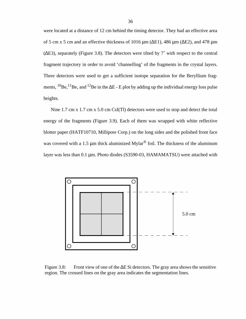
were located at a distance of 12 cm behind the timing detector. They had an effective area

of 5 cm x 5 cm and an effective thickness of 1016 µm (∆E1), 486 µm (∆E2), and 478 µm

(∆E3), separately (Figure 3.8). The detectors were tilted by 7˚ with respect to the central

fragment trajectory in order to avoid ‘channelling’ of the fragments in the crystal layers.

Three detectors were used to get a sufficient isotope separation for the Beryllium frag-

ments, 10Be,11Be, and 12Be in the ∆E - E plot by adding up the individual energy loss pulse

heights.

Nine 1.7 cm x 1.7 cm x 5.0 cm CsI(Tl) detectors were used to stop and detect the total

energy of the fragments (Figure 3.9). Each of them was wrapped with white reflective

blotter paper (HATF10710, Millipore Corp.) on the long sides and the polished front face

was covered with a 1.5 µm thick aluminized Mylar® foil. The thickness of the aluminum

layer was less than 0.1 µm. Photo diodes (S3590-03, HAMAMATSU) were attached with

5.0 cm

Figure 3.8: Front view of one of the ∆E Si detectors. The gray area shows the sensitiveregion. The crossed lines on the gray area indicates the segmentation lines.

37

silicone rubber glue (RTV615, GE) at the back end of each crystal and covered with white

Teflon® tape for light sealing and for improving light reflection.

3.5 Electronics and Data Acquisition

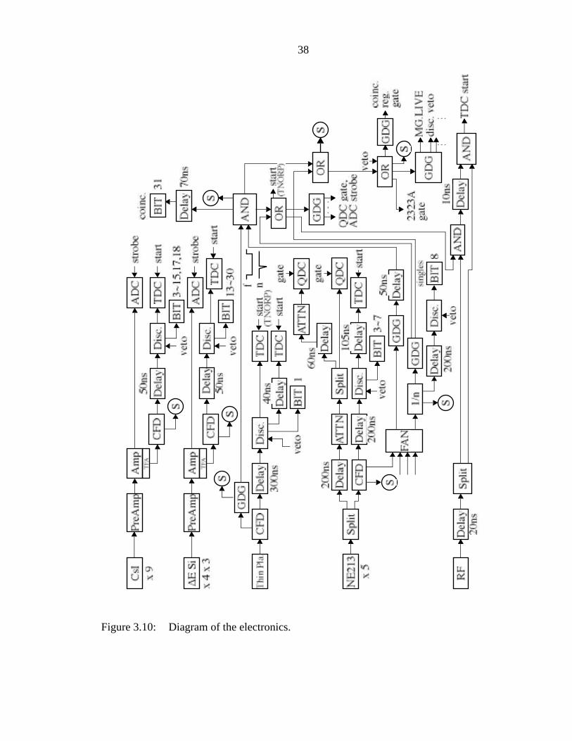
Figure 3.10 displays the schematics of the electronics used for the signal processing. The

photo diodes attached to the CsI(Tl) crystals E detector had a full depletion voltage of 70

Volts and a maximum voltage of 100 Volts. They were reversely biased with 80 Volt

through the preamplifiers. The signal picked up by the preamplifier was passed to the linear

amplifier with a 3 µs shaping time. The peak height of the outputs of the linear amplifiers

was proportional to the kinetic energy of the detected projectile fragment. These energy

signals were recorded with a peak sensitive ADC (AD811, ORTEC). The fast time signal

outputs of the linear amplifier were sent to Constant Fraction Discriminators (CFD: TC455,

1.7 cmaluminized

Mylar®

photo diode

white blotter paper

Figure 3.9: Structure of CsI(Tl) E detector array. Each of the nine crystals werewrapped with white blotter paper independently to optically isolate them from each other.

38

Figure 3.10: Diagram of the electronics.

39

TENNELEC) to create TDC stop signals relative to the K1200 cyclotron RF time and to

create a bit for each E signal.

Basically the same signal processing was used to operate the three quadrant ∆E Si de-

tectors. The shaping time of the linear amplifiers was set to 1 µs for the ∆E detectors. ∆E1,

∆E2, and ∆E3 detectors were biased with 90 Volts, 30 Volts, and 42 Volts, respectively.

The fast plastic timing scintillator was attached to a photomultiplier tube. The signal

from the tube was fed to a CFD, and one of the outputs was used as part of the fragment -

neutron coincidence condition. The pulse width of the CFD output for the fast plastic

timing detector signal, which was fed to the coincidence AND, was ~ 200 ns. The other

outputs of the CFD were used to set a bit for each event detected in the fast plastic detector

and to generate a stop signal for a TDC to measure the time of flight relative to the cyclotron

RF and the neutron time signal, respectively.

The neutron liquid scintillator detectors were also equipped with photomultiplier tubes.

The signals from the tubes were split into an energy and time branch. The energy signal

from each detector was integrated in two separate charge sensitive ADC (QDC) channels.

Two differently gated signal charge integrations (tail and total) were necessary to achieve

pulse shape discrimination between γ-rays and neutrons. Details of this technique will be

discussed in Chapter 4. In the time branch, the signal from the neutron detectors were sent

to a CFD and created time signals. They were passed to TDC stops and bits for each neutron

detector as well as a bit for downscaled neutron singles. A short (~ 5 ns) signal was also

created from the time signals and was fed to the neutron-fragment coincidence AND. Since

it was much shorter than the other coincidence condition signal from the thin fast plastic

detector (~ 200 ns), time of the neutron - fragment coincidence signals was dominated by

40

the neutron time. The downscaled singles formed one event type of the master gate, togeth-

er with the main event type of coincidence events.

The RF time signal from the K1200 cyclotron was used as a time reference. The original

RF signal had a sinusoidal shape and a frequency of 18.4 MHz, leading to repeated beam

bursts at ∆t = 54.4 ns. The RF signal was used to start all of the TDCs except the TDC for

the TNORP (see 4.2.3) signals, in coincidence with a “master gate” signal consisting of the

neutron singles and neutron-fragment coincidences. A veto signal blocked the data acqui-

sition during the busy time of the frontend processor.

Finally, accepted events were written to 8 mm tapes and analyzed online, using the

standard NSCL data acquisition system [Fox89, Fox92].

41

Chapter 4

Data Analysis

4.1 Overview

The off-line analysis of the data was performed with the NSCL data analysis program

SARA [Fox89, Fox92]. The experiment consisted of four parts. First, fragment singles

were recorded for energy calibration of the E detectors and gain matching of ∆E detectors.

The second part included neutron singles runs for gain matching of the neutron detectors

and calibration of the neutron times. In the third part, coincidence events of neutrons and

fragments were measured to obtain the relative velocity spectra. For the forth part, shadow

bar runs were conducted to measure the neutron background. The calibration of the ener-

gies (E), energy losses (∆E), and time of flights (TOF) were performed off-line. Subse-

quently, calibrated ∆E-E particle identification (PID) histograms were created. Software

gates were drawn for three different elements (He, Li, and Be) on the ∆E-E particle identi-

fication (PID) plot and the data was filtered into three sets based on these gates. Individual

isotope (6He, 9Li, and 12Be) gates were obtained from the filtered data using both the ∆E-

E and the ∆E-TOF plot. Neutrons were separated from γ-rays by pulse shape discrimination

technique (see section 4.3.1). A relative velocity spectrum of 7He → 6He + n was created

from the filtered data. The neutron decay energy and the width of 7He are well known

42

[Ajz88] and thus could be used as a calibration reaction. The time zero constants for the

neutron TOF of each neutron detector in the data analysis code were adjusted to match the

centers of the spectra with the simulations. The relative velocity spectra of 10Li → 9Li + n

and 13Be → 12Be + n were then obtained from the filtered data and compared to the Monte

Carlo simulations to extract the decay energies and the widths.

4.2 Calibration of Detectors

4.2.1 Calibration of the Fragment Telescope

The resolution of the E detectors was crucial because the energy information of the frag-

ments was used to calculate the fragment velocity and also indirectly the neutron velocity.

For the energy calibration of the CsI(Tl) energy detectors and the gain matching of an en-

ergy loss in the Si quadrant segmented detectors, calibration beams of isotopes with mass-

to-charge ratio equal to three (6He, 9Li, and 12Be) were used. The calibration beams were

Table 4.1: Calibration beam energies for different target thicknesses.

27Al target thickness

[mg/cm2]

Bρ [T•m]

Kinetic energy of a fragment [MeV]

6He 9Li 12Be

370 3.797 445.8 668.7 891.6

247 3.834 454.2 681.4 908.5

177 3.865 461.5 692.2 922.9

81 3.909 471.6 707.4 943.2

33 3.929 476.1 714.2 952.2

3.4 3.941 479.1 718.6 958.2

43

created by fragmentation of a primary 18O beam with a kinetic energy of 80 MeV/nucleon

on various Al targets. The A1200 mass analyzer was used to separate isotopes with mass-

to-charge ratio equal to three. A momentum slit located at image1 in the A1200 was used

to limit the momentum spread of the calibration beam to 0.25% (FWHM) and 1.0%

(FWHM). This corresponds to 0.5% (FWHM) and 2.0% (FWHM) spread in energy.

Six 27Al targets with different thicknesses were used to produce six different energies

of calibration beams. The magnetic rigidities (Bρ) of the secondary beam were calculated

using the code INTENSITY [Win92]. The different 27Al target thicknesses, the Bρs of the

A1200 mass analyzer, and corresponding total kinetic energies of the fragments of the cal-

ibration beam are shown in Table 4.1. The total kinetic energy of the calibration beam was

calculated using the relation between kinetic energy T [MeV], mass number of the nucleus

A, atomic number of the nucleus Z, and Bρ [T-m],

(4.1)

where

[MeV]. (4.2)

Two-dimensional histograms of the fragment energy loss versus the fragment time of

flight which was measured between the cyclotron RF and a thin plastic timing detector

(∆E1,2,3 vs. TOF), and the fragment energy loss versus the fragment total energy (∆E1,2,3

vs. E) were created from the data to identify the isotopes in the calibration beam. Examples

are shown in Figure 4.1 and Figure 4.2. For the ∆E detectors, the number of charge carriers

created within a detector of small thickness x is proportional to the specific energy loss

dE/dx and x [Kno89]. The specific energy loss of nonrelativisitic charged particles of

mass m and charge Ze is expressed in Bethe’s formula:

T A u2

Bρ299.7925ZA

-------------------------- 2

+ uA–=

u 931.49432=

44

Time of flight

Figure 4.1 Two dimensional histogram of energy loss in the ∆E2 detector’s quadrantnumber 1 versus time of flight of the fragments. m/q = isotopes are selected using theA1200 mass analyzer.

A/Z=3 line

6He

9Li

12Be

15B

8Li

11Be

E

Figure 4.2: Two dimensional histogram of energy loss in the ∆E2 detector’s quadrantnumber 1 versus total energy in the E3 detector of the fragments. The large square gate inthe plot was applied to select the valid signal for a projection.

6Ηe

9Li

12Be

8Li

11Be

15Β

45

(4.3)

where C1 and C2 are constants. It shows that the energy loss is very sensitive to the mZ2

value but only mildly dependent on the particle energy E. For the E detectors, it is obvious

that the number of charge carriers created within a detector is proportional to the total ki-

netic energy E of the incident charged particles. This different dependence of the signal in

the ∆E and E detectors allowed the isotope separation.

The A1200 selects isotopes according to their momentum over charge ratio. The force

FMAG on a charge q moving with velocity v in magnetic flux B is,

(4.4)

where FMAG, v, and B are all perpendicular to each other. This charged particle moves

along the circular trajectory with a radius ρ because of this force and the centripetal force

Fcen of circular motion can be expressed in the form:

. (4.5)

Since FMAG = Fcen,

(4.6)

which leads to

. (4.7)

The centroid of the velocity distributions are equal for all the isotopes in a secondary beam.

For a given Bρ value of the A1200 isotopes with the same mass-to-charge ratio m/q have

the same velocities v. For example, isotopes with m/q = 3 were selected and they all had

the same time of flight (the same velocities v) as shown in Figure 4.1.

In the figure, some isotopes with m/q ≠ 3 are also observed (8Li, 11Be, etc.). In the 8Li

case, the mass number is 1 less than the chosen m/q = 3 groups. From Equation 4.7, the

Edxd

------ C1mZ2

E---------- C2

Em----ln=

FMAG qvB=

Fcenmv2

ρ----------=

qvBmv2

ρ----------=

Bρ mvq

--------pq---= =

46

velocity v of 8Li has to be greater than the chosen group to yield the same Bρ to be selected.

8Li was observed in Figure 4.1 at the shorter time of flight (higher velocity v) side than 9Li.

The energy of those particles are expressed as E = p2/2m and as can be seen in Figure 4.2,

8Li has larger energy since the selected 8Li group has lower mass number than 9Li and the

same momentum as 9Li.

A projection of the two dimensional gates on m/q = 3 isotopes on the E axis is shown

in Figure 4.3. The location of the peaks for each isotopes for the six different energies were

fitted quadratically by a least square method as a function of the kinetic energy of the cal-

ibration beams to extract calibration constants for 6He, 9Li, and 12Be isotopes, individually.

The energy resolution of the E detectors was ~ 0.5% (FWHM). These fits are shown in Fig-

ure 4.4, 4.5, and 4.6 (6He, 9Li, and 12Be). The energy detector E2 showed an abnormal be-

havior and it was thus omitted from the later data analysis.

103

102

101

100

70 11090 130 150 170 19050

6He 9Li12Be

15B

Figure 4.3: Energy spectrum of the calibration beam with an A/Z=3 gate.

Energy [a.u.]

47

Figure 4.4: Quadratic fitting for energy calibration of the 6He fragment for each E de-tector. The E2 detector was omitted due to its nonlinear behavior.

Energy [MeV]

48

Energy [MeV]

Figure 4.5: Quadratic fitting for energy calibration of the 9Li fragment for each E de-tector. The E2 detector was omitted due to its nonlinear behavior.

49

Figure 4.6: Quadratic fitting for energy calibration of the 12Be fragment for each E de-tector. The E2 detector was omitted due to its nonlinear behavior.

Energy [MeV]

50

The code STOPX [Oak92] was used to calculate the energy loss of the calibration

beams in the ∆E detectors. Peak channel positions in the one dimensional ∆E spectra of

6He, 9Li, and 12Be isotopes were recorded (Figure 4.7) and fitted quadratically as a function

of the calculated energy loss by the least square method. The calculated energy loss of the

three isotopes were used together to align the peak positions of the same isotope between

the all ∆E detectors. Using the constants obtained from the fitting, pseudo parameters were

created in the data analysis code for each ∆E1, 2, and 3 signals to align the peaks of the

isotopes on the one dimensional pseudo parameter plots. Then the plots of ∆E1, ∆E2, and

∆E3 pseudo parameters were added to obtain a total ∆E information and used for the par-

ticle identification in the two dimensional plots (∆E-E, ∆E-TOF).

Figure 4.7: Energy loss spectrum of the calibration beam with A/Z=3 gate.

Energy loss [a.u.]

100

101

102

0 50 100 150 200 250

51

4.2.2 Neutron Detector Calibration

The scintillation material (NE 213) in the neutron detectors is sensitive to both neutrons and

γ-rays. We used pulse shape discrimination [Hel88] to identify neutrons and γ-rays. The to-

tal pulse (total) and the tail of the pulse (tail) from the photomultiplier tubes of neutron de-

tectors were integrated separately (Figure 4.8). The same gate width of 400 ns was used to

integrate the charge of those two channels but a different part of the signal was integrated

by delaying one signal with respect to the other by 60 ns (see Figure 3.10). Because of the

difference of the interactions in the scintillation material, a neutron signal has a larger tail

compared to a γ-ray signal with a similar pulse height. This difference separates two parti-

cles on the two dimensional plot of tail vs. total signals. A 239Pu-Be neutron-γ-ray source

(0 ~ 10 MeV for neutrons and 4.44 MeV for γ-rays) and a 60Co γ-ray source (1.173 MeV

400 ns

60 ns

QDC gate

Tail charge integration

Total charge integration

(original signal)

(delayed by 60 ns)

Figure 4.8: Timing diagram of the neutron signals and the QDC gate. Shaded areasshow the integrated part of the neutron signal.

52

and 1.332 MeV) were used to obtain the two dimensional plot shown in Figure 4.9 and the

tail gate time and attenuation ratio of total signal were adjusted to maximize the separation

of the two groups.

The gains of the five individual neutron detectors were matched with a 60Co γ-ray

source (1.173 MeV and 1.332 MeV) and a 239Pu-Be neutron-γ-ray source (4.44 MeV). The

projection of the condition around the γ-ray group of the two dimensional plot on the ener-

gies is shown in Figure 4.10. The high voltage biases were adjusted to match the compton

edges of the five neutron detectors for the 60Co (0.963 MeV and 1.118 MeV) and for the

239Pu-Be (4.198 MeV). Those were -1440 V (N1), -1400 V (N2), -1450 V (N3), -1400 V

(N4), and -1400 V (N5). For the experiment the neutron detector signals were then attenu-

ated to be able to accommodate the highest neutron energy signals (~ 80 MeV) within the

dynamic range of the QDC.

Figure 4.9: Two dimensional plot of the neutron detector signal. A 239Pu-Be sourcewas used to supply γ-rays and neutrons along with 60Co γ-ray source.

Total

neutrons

γ-rays

53

4.2.3 Time Calibration

All TDCs were calibrated with a time calibrator electronics module which created a cali-

brated time signal (multiple of 10.0 ns) over the TDC range (~ 200 ns). Six positions of the

calibration peak for each TDC were recorded and linearly fitted as a function of time in ps.

All TDCs had a time gain of ~ 100 ps/ch. The fragment time information was used for the

particle identification.

The ‘or’ of all neutron detectors started a TDC which was stopped by a coincidence

fragment in the thin fast plastic detector and recorded in a TDC (TNORP). If tn is a neutron

TOF and tf is a fragment TOF, then TNORP is defined as

TNORP = (tf + Cf) - (tn + Cn) (4.8)

where Cf and Cn are constants. Rearranging this equation yields,

Energy [a.u.]

discriminator threshold

compton edge of 239Pu-Be source

Figure 4.10: Compton edges of a 60Co source and a 239Pu-Be source in a one dimen-sional plot of the neutron total signal. It was obtained by using the γ-ray condition estab-lished in the two dimensional plot (Figure 4.9).

unresolvedcompton edgesof 60Co source

0 20 40 60 80 100 120 1400

200

400

600

800

1000

54

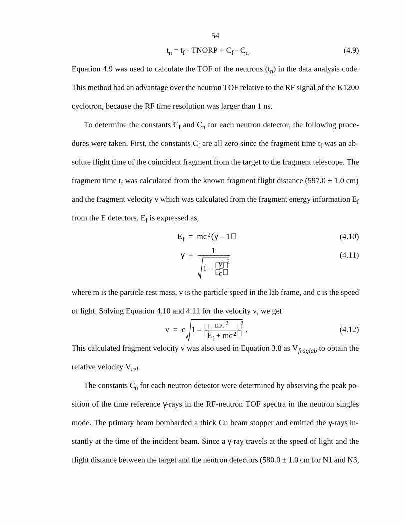
tn = tf - TNORP + Cf - Cn (4.9)

Equation 4.9 was used to calculate the TOF of the neutrons (tn) in the data analysis code.

This method had an advantage over the neutron TOF relative to the RF signal of the K1200

cyclotron, because the RF time resolution was larger than 1 ns.

To determine the constants Cf and Cn for each neutron detector, the following proce-

dures were taken. First, the constants Cf are all zero since the fragment time tf was an ab-

solute flight time of the coincident fragment from the target to the fragment telescope. The

fragment time tf was calculated from the known fragment flight distance (597.0 ± 1.0 cm)

and the fragment velocity v which was calculated from the fragment energy information Ef

from the E detectors. Ef is expressed as,

(4.10)

(4.11)

where m is the particle rest mass, v is the particle speed in the lab frame, and c is the speed

of light. Solving Equation 4.10 and 4.11 for the velocity v, we get

. (4.12)

This calculated fragment velocity v was also used in Equation 3.8 as Vfraglab to obtain the

relative velocity Vrel.

The constants Cn for each neutron detector were determined by observing the peak po-

sition of the time reference γ-rays in the RF-neutron TOF spectra in the neutron singles

mode. The primary beam bombarded a thick Cu beam stopper and emitted the γ-rays in-

stantly at the time of the incident beam. Since a γ-ray travels at the speed of light and the

flight distance between the target and the neutron detectors (580.0 ± 1.0 cm for N1 and N3,

Ef mc2 γ 1–( )=

γ 1

1vc---

2–

------------------------=

v c 1mc2

Ef mc2+----------------------

2–=

55

579.0 ± 1.0 cm for N2 and N4, and 592.0 ± 1.0 cm for N5) are known, we could calculate

the time offset of the TDC’s.

4.3 Coincidence Fragment Spectra

All the neutron-fragment coincidence data was filtered into three groups (He, Li, and Be)

and were copied to three 8 mm tapes, one for each group. Filtering conditions were estab-

lished in two dimensional plots of the gain matched energy loss versus the calibrated ener-

gy (∆E-E) for each fragment group since each isotope, 6He, 9Li, and 12Be had its own

energy calibration constants, respectively. No gate was applied to the two dimensional plot

of the neutron detector signal (tail vs. total) for the filtering.

When coincidence events are recorded, it is inevitable to record chance coincidence

events (randoms) simultaneously since the coincidence gate triggered by the fragments is

~ 200 ns wide and once it is opened, any type of neutron detector signal can satisfy the co-

incidence condition (see Figure 3.10 and 4.11). The RF signal from the K1200 triggered a

TDC start for measuring the fragment time only when a master gate trigger existed. The

master gate consisted of coincidences of neutrons with fragments or downscaled neutrons

where the time was determined by the neutrons. The neutron detector signal times could

have a ~ 200 ns range to be considered as a coincidence event and the gate for the RF was

~ 100 ns wide (see Figure 4.11). If the fragment time spread is considered, the possible neu-

tron time range to satisfy the coincidence condition would be ~ 150 ns. The time relations

(Figure 4.11) show that one of four different RF triggers could start the TDC. The most

prominent peak (reals) in the fragment TOF spectrum contained the fragments from both

real and random coincidence events. Reals and randoms gates for the each isotope (6He,

56

Figure 4.11: The relation of the fragment time signal, the neutron detector signal, and theRF time signal. The earliest and latest possible neutron signal have margins of ~ 25 ns fromthe edge of the fragment signal to take a fragment time spread into account.

200 ns

100 ns

100 ns

fragment time

earliest possibleneutron time

latest possibleneutron time

earliest possibleRF gate bymaster gate

latest possibleRF gate bymaster gate

RF time

54.4 ns

four possible TDC start triggers

delay

delay

57

9Li, and 12Be) in ∆E vs. TOF plots as well as individual isotope gates (6He, 9Li, and 12Be)

in E vs. ∆E plots were established using each filtered data sets. It was necessary to subtract

the randoms from the reals to extract the shape of the relative velocity spectrum only from

the real coincidence events.

4.3.1 He group

The filtered data of the He group was used to observe the known state of 7He. To select the

6He group from the one neutron decay of 7He, energy loss versus total energy plot (∆E-E,

Figure 4.12) and energy loss versus time of flight plot (∆E-TOF, Figure 4.13) were used.

The 6He isotope gate, the 6He reals gate, and the 6He randoms gate are indicated in the fig-

ures. The 6He nucleus has a long enough lifetime (~ 807 ms) to be observed in the fragment

telescope. The neighbors of the 6He (5He and 7He) are both unbound which makes it easy

Figure 4.12: ∆E_1 (first quadrant of ∆E) vs. E3 plot of He group. The oval contourshows a 6He gate.

280 360 440 520 600 6800

20

40

60

80

E [MeV]

58

to isolate the 6He group in the two dimensional plots.

4.3.2 Li Group

To study 10Li states, the coincidence events of a neutron and a 9Li were separated from the

other events. Similar to the 7He case, energy loss versus total energy plot (∆E-E, Figure

4.14) and energy loss versus time of flight plot (∆E-TOF, Figure 4.15) were used. 10Li itself

was not observed on the ∆E-E and the ∆E-TOF plot because it is a neutron unbound nucle-

us. 8Li and 9Li have long enough lifetimes (~ 838 ms and ~178 ms) to be detected in the

fragment telescope. Like in the 7He case of the previous section, the reals and the randoms

of the 9Li were selected by the gates in the ∆E-TOF spectra.

The ∆E-E plots were handled similar to the 7He case except that E5, one of the CsI(Tl)

E detectors was excluded since it did not have a sufficient isotope separation between the

Figure 4.13: ∆E_1 (first quadrant of ∆E) vs. TOF (thin plastic time) plot of He group.The contour gates show the 6He reals gate and the 6He randoms gate.

0 40 80 120 160 2000

20

40

60

80

TOF [ns]

reals randoms

59

Figure 4.14: ∆E_1 (first quadrant of ∆E) vs. E3 plot of the Li group. The contour showsa 9Li isotope gate.

520 600 640 680 720 76030

40

50

60

70

80

90

100

110

120

E [MeV]

Figure 4.15: ∆E_1 (first quadrant of ∆E) vs. TOF (thin plastic time) plot of Li group.The contour gates show the 9Li reals gate and the 9Li randoms gate.

104 120 136 152 168 184 20040

60

80

100

120

TOF [ns]

reals randoms

60

8Li and 9Li group. This was probably due to abnormal scattering at the center of the ∆E

detectors (see Figure 3.8), since the E5 detector was located right behind the center crossing

of the segmentation lines of the ∆E detectors (see Figure 3.9). Thus, the E5 related Li data

was omitted in the later analysis.

4.3.3 Be Group

The filtered data of the Be group was used to select neutron decay events of 13Be. Energy

loss versus total energy plot (∆E-E, Figure 4.16) and energy loss versus time of flight plot

(∆E-TOF, Figure 4.17) were used to select the12Be group from the one neutron decay of

13Be. Unlike 13Be, the neighbors 11Be and 12Be have long enough lifetimes (~ 14 s and ~

24 ms) to be detected in the fragment telescope. The E5 related Be data were also omitted

Figure 4.16: ∆E_1 (first quadrant of ∆E) vs. E3 plot of the Be group. The contour showsa 12Be isotope gate.

50

70

90

110

130

150

170

190

457 571 686 800 914 1029 1143 1257

E [MeV]

61

in the later analysis from the same reason mentioned in the Li section.

4.4 Simulation of Experiment

Monte Carlo simulations were performed to calculate the relative velocity spectrum for the

one neutron decay of 7He, 10Li, and 13Be, respectively. The decay of each fragment was

initially considered in the center of mass (CM) frame of the daughter fragment and the neu-

tron. The decay direction was assumed to be isotropic in the CM frame and a Breit Wigner

lineshape of the form [Lan58]

(4.13)

where

(4.14)

Figure 4.17: ∆E_1 (first quadrant of ∆E) vs. TOF (thin plastic time) plot of Be group.The contour gates show the 12Be reals gate and the 12Be randoms gate.

104 120 136 152 168 184 20070

90

110

130

150

170

TOF [ns]

reals randoms

σdEd

-------Γ E( )

E Er–( )2 14--- Γ E( )[ ]2+

-----------------------------------------------------=

Γ E( )kPl E( )

krPl Er( )--------------------Γ0=

62

was used. Pl(E) was the l-dependent neutron penetrability function, and Γ0 = Γ(E = Er) was

the width at the resonance energy Er.

The decay energy of each event was transformed into the center of mass velocity of the

neutron and the fragment, and then into the laboratory frame velocity of the neutron and the

fragment. In the next step, the decay direction of the fragment in the laboratory frame, was

compared with the data in an acceptance file which was calculated using the RAYTRACE

[Kow87] code. It contained the data of valid directions of the fragment velocity in the lab-

oratory frame at the target to reach the fragment telescope. The magnet settings of the qua-

drupole and the dipole, the location of the 11˚ beam pipe and the Cu collimator (see Figure

3.3, 3.7) were considered in the calculation. The events which had fragment velocity direc-

tions outside this acceptance were excluded. The direction of the neutron velocity in the

laboratory frame was checked and only the events which hit the neutron detector array were

used to calculate the relative velocity. The neutron detector efficiency was taken into ac-

count for the histogramming of the relative velocity spectrum by looking up an efficiency

file which contained efficiency factors for each neutron energy. This file was created by the

KSUEFF [Cec79] code.

A simulation for the neutron decay of 7He was executed first to set the parameters of

the Monte Carlo simulations and constants in the data analysis code, since 7He has a well

established ground state energy (Er = 440 ± 30 keV) and width (Γ0 = 160 ± 30 keV)

[Ajz88].

The input parameters of the simulation were set in the following way. The TOF

resolution (σ = 0.057ns) of the daughter fragment 6He was calculated from the energy

resolution of the CsI(Tl) E detectors because it was calculated from the energy information.

63

The centroid of the momentum distribution (2733.3 MeV/c for 7He) and the width of the

scattering angle (70.47 mrad for 7He) of the fragmentation product at the target (9Be, 94

mg/cm2) were predicted using INTENSITY. The momentum spread of the fragmentation

product (σ = 3.54% for 7He) for the simulation was set to match the actual spread of

experimental data of the coincidence runs. After setting these parameters, the TOF

resolution of the neutron was found by reduced chi-square ( ) minimization of the fit of

the calculated relative velocity spectrum to the measured spectrum. Figure 4.18 shows the

minimum of a neutron TOF resolution at σ ~ 0.70 ns.

For the decay of 10Li to 9Li + n and 13Be to 12Be + n, the simulations were carried out

for different combinations of decay energy, width, and angular momentum. The TOF

resolution of the fragment and the neutron were fixed to the value which was established

from the 7He neutron decay simulation. The centroid of the momentum distribution (3901.9

χν2

0.8

0.9

1

1.1

1.2

0.5 0.6 0.7 0.8 0.9 1 1.1

χν2

ntres

[ns]

Figure 4.18: χν2 versus neutron TOF resolution plot. χν

2 is for the fit of the 7He neutrondecay simulation and the data. The minimum χν

2 of (best fit) is at tnres ~ 0.70 ns.

64

MeV/c for 10Li and 5068.8 MeV/c for 13Be) and the width of the fragment scattering angle

(53.90 mrad for 10Li and 42.38 mrad for 13Be) were also calculated by INTENSITY. The

middle of the momentum distribution of the fragmentation products (σ = 3.38% for 10Li

and σ = 3.22% for 13Be) were obtained in a same way as in the 7He case.

65

Chapter 5

Results and Discussion

5.1 Selection of The Valid Events

The valid events for the relative velocity (Vrel = Vn - Vf, Equation 3.8) spectra were select-

ed with the ∆E-E isotope gates, with the ∆E-TOF isotope gates for reals and randoms, and

with the neutron gates on the two dimensional plot of the neutron signals (see previous

chapter). Relative velocity spectra were obtained for each isotope, for each neutron detec-

tor, and for reals and randoms by scanning the filtered data for the same Z group. The rel-

ative velocity spectra of randoms were subtracted from the reals, and all the subtracted

spectra for the different neutron detectors were summed to obtain the total relative velocity

spectrum for each isotope.

5.2 The Relative Velocity Spectrum of 7He

7He has a p3/2 ground state with a neutron separation energy of Sn = -440 ± 30 keV and a

Γ = 160 ± 30 keV width [Ajz88]. Figure 5.1 shows the relative velocity spectrum for 6He

+ n coincidence events which were collected simultaneously with the 9Li + n and the 12Be

+ n events. The open circles with the error bars in the figure represent the data and the solid

line is the simulated decay of the ground state of 7He (dotted) superimposed upon an

66

Figure 5.1: The relative velocity spectrum for 6He + n coincidence events. The circleswith the error bars are the data. The dashed line shows the estimated background. The dot-ted line is the simulated decay of ground state of 7He without the background and the solidline is a sum of the background and the simulation.

Vn - Vf [cm/ns]

67

estimated background (dashed). The known decay energy and width were used in the

simulation. The two peaks in the relative velocity spectrum correspond to forward (positive

Vn-Vf) and backward (negative Vn - Vf) emitted neutrons. Vn

- Vf = 0.0 cm/ns indicates

zero decay energy (Q-value is zero).

The precise source of the background for the neutron-fragment coincidence events is

unknown. The background has previously been investigated using the distribution for a

thermal neutron source of the form [Deá87]. This thermal source lead to a

near-Gaussian shape background in the Monte Carlo simulation, thus Heilbronn [Hei90]

treated them in general as a simple broad Gaussian which had a centroid at some nonzero

relative velocity value. This approach was also adapted in the present case. The parameters

of the background Gaussian were obtained by fitting the data to the simulation which as-

sumed to be a sum of a broad Gaussian and the ground state decay simulation of 7He, leav-

ing the centroid, width, and amplitude of the Gaussian and the amplitude of the decay

simulation as fitting parameters.

In Figure 5.2, the solid line shows the calculated lineshape by the Breit-Wigner form

(Equation 4.12) with the l-dependent neutron penetrability factor, which was used for the

simulation of the ground state decay of 7He. The neutron separation energy of Sn = -440

keV, width of Γ = 160 keV, and l = 1 were used for the calculation. The result for the l = 0

with the same parameter as the l = 1 case is shown in the figure with the dashed line for

comparison. The lower energy part of the l = 1 lineshape is clearly suppressed compared to

the l = 0 case because of the l dependent penetrability factor.

Previously, Kryger et al. [Kry93] employed the same experimental method of sequen-

tial neutron decay spectroscopy (SNDS) at 0˚ to investigate the ground state of 10Li. Kryger

E E T⁄–( )exp

68

Figure 5.2: The Breit-Wigner lineshapes of 7He state at r = 440 keV with the widthof Γ = 160 keV. The solid line shows the actual case with the angular momentum l = 1. Forthe comparison, l = 0 case is shown with the dashed line. The low energy region of the peakfor the l = 1 case is suppressed compared to the l = 0 case.

Decay energy Er [MeV]

69

et al. used the cyclotron RF as the start for the TOF for both the neutrons and the fragments

to calculate the neutron velocity Vn and the fragment velocity Vf and obtained the relative

velocity Vrel (= Vn - Vf). The time resolution for the neutron TOF and the fragment TOF

were both σtn = σtf = 0.89ns. The current experiment used the fragment energy information

from the E detectors to calculate the Vf to utilize the superior energy resolution (0.49%,

FWHM), corresponding to a fragment TOF resolution of σtf = 0.057ns. The fragment TOF,

calculated from the energy, and the TNORP were used to calculate the TOF of neutrons

yielding a resolution of σtn = 0.70 ns. The resolution was thus significantly improved for

the current experiment. The width of the peaks of 6He + n coincidence events were also

used to confirm the experimental resolutions. Figure 5.3 shows a comparison of the relative

velocity spectrum calculation using the different timing resolution. The dotted line shows

the perfect resolution case (neutron TOF resolution; σtn = 0.00 ns, fragment timing resolu-

tion; σtf = 0.00 ns). The dashed line shows the spectrum with the resolution of the setup

used by Kryger et al. (σtn = 0.89 ns, σtf = 0.89 ns). The solid line shows the spectrum with

the resolutions of the current experiment (σtn = 0.70 ns, σtf = 0.057 ns). As one can see from

the figure, the width of the peaks in the relative velocity spectrum of the data is broadened

by an finite experimental time resolutions. The current experiment clearly shows the im-

provement in the resolution of the relative velocity.

5.3 The Relative Velocity Spectrum of 10Li

The first measurement by Wilcox et al. was reported in 1975 observing a lowest 10Li un-

bound state at Er = 800 ± 250 keV and Γ = 1200 ± 300 keV. Then the presence of a p-wave

state at Er = 420 ± 50 keV and Γ = 800 ± 60 keV was reported by Bohlen et al. [Boh93]

70

Figure 5.3: The relative velocity spectrum simulation of 7He → 6He + n decay for thedifferent time resolutions. The dotted line shows a case of perfect resolution (σtn = 0.00ns, σtf = 0.00 ns). The solid line shows a case of a current experimental resolution (σtn =0.70 ns, σtf = 0.057 ns). The dashed line shows a case of the experiment by Kryger et al.(σtn = 0.89 ns, σtf = 0.89 ns).

Vn - Vf [cm/ns]

71

and interpreted as the ground state. However, a low-lying s-wave state at Er = 150 keV and

Γ0 < 400 keV by Amelin et al. [Ame90] and also by Kryger et al. [Kry93] were reported

as the 10Li ground state. Young et al. [You94] observed a p-wave state similar to Bohlen’s

value (Er = 538 ± 60 keV) and, in addition, evidence of the lower lying state (Er ~ 100 keV).

Ostrowski et al. recently reported a new value (Er = 240 keV) as a p-wave ground state

[Ost96]. Our newly obtained data allowed us to determine if this state could potentially cor-

respond to the state observed by Kryger et al.

Figure 5.4 shows the relative velocity spectrum of the 9Li and neutron coincidence

events. The dotted line indicates an estimated broad Gaussian background. The dashed

lines show a simulated p-wave state (side peaks) at Er = 538 keV, Γ0 = 358 keV, corre-

sponding to the result reported by Young et al. [You94] and a simulated s-wave state (cen-

tral peak) at Er = 50 keV, Γ0 = 241 keV. The positions of the side peaks in the data matches

the simulation with the Young’s value quite well, however the statistics is not sufficient to

extract the values from a fit to the data. The p-wave state reported by Bohlen et al. (Er =

420 keV) was also tried for the simulation and yielded similar side peaks in the relative ve-

locity spectrum as the Young’s state (Er = 538 keV). Therefore, we consider these two

states as one state. In the new report by Ostrowski et al.[Ost96], this state was also assumed

as a first excited state for a fitting purpose. Thus the state at Er = 538 keV (Young’s value)

was assumed and included in the subsequent χ2 fitting procedures.

To extract the decay energy and the width of the initial state for the central peak, sim-

ulations were performed and fitted to the data. For the 10Li initial state, neutron decays cor-

responding to states of l = 0 case and l = 1 case were considered. Each central peak

simulation had a certain combination of the decay energy Er, the width Γ0, and the l value

72

Figure 5.4: The relative velocity spectrum of 10Li → 9Li + n. The convention of thedata point and the Gaussian background are the same as the 7He spectrum. The dashed sidepeaks are the simulation of the p-wave state at Er = 538 keV reported by Young et al. Thedashed central peak is the simulation with l = 0, r = 50 keV, Γ0 = 241keV. This is the fitat minimum for the s-wave neutron.χν

2

Vn - Vf [cm/ns]

73

of the initial state neutron in 10Li. The output file of the central simulation was used along

with the p1/2 state at 538 keV for the fitting. The amplitude of these two simulations and

the parameters of the Gaussian background (amplitude, centroid, and width) were set to be

free parameters and the best fit was searched to minimize the reduced chi-square with

a computer routine [Bev69].

surfaces as a function of Γ0 and Er were extracted in Figure 5.6 and 5.9. The overall

minimums of the reduced chi-square are indicated with x. The reduced chi-square

value was considered to be a tolerance limit of a good fit. The upper lim-

its of the width Γ0 for each decay energy Er were calculated by setting the spectroscopic

factor to the theoretical limit which is unity in a formula of a broad resonance [Rol88],

(5.1)

where E = Er in this case since Γ0 = Γ(E = Er) was used for the simulation parameter, Rn is

the nuclear radius, and Pl is the l dependent penetrability factor. This limit is referred to as

the Wigner limit. The solid lines shows the Wigner limit and the dashed lines correspond

to constant values of , , and as indicated in the fig-

ures.

In the relative velocity spectrum, the distance along the abscissa from 0.0 cm/ns is

directly related to the relative decay energy Er as described in Equation 3.3. Therefore, the

existence of the central peak inside the two side peaks of the 538 keV p-wave state in the

relative velocity spectrum implies another state with a lower decay energy than the p-wave

state and/or with a very broad width.

The widths of the peaks in the relative velocity spectra are related to the width of the

initial state and the final state of the decay as well as the experimental resolution. For the

χν2

χν2

χνmin2

χν2 χνmin

2 0.5+=

l2

Γl E( ) 2hRn------

2Eµ

------- 1 2⁄

Pl E Rn,( ) l2

=

χν2 χνmin

2 0.5+ χνmin2 1.0+ χνmin

2 1.5+

74

final states, only the bound states matter for the analysis. 9Li has only two bound states

which are the ground state and the first excited state (Ex = 2.691 MeV). As final states of

the10Li neutron decay, the widths of these two states are very narrow [Ajz88], and their

contribution to the width of the peaks in the relative velocity spectra were negligible

compared to the contribution from the width of initial states and the finite experimental

resolution.

The present experimental method was only sensitive to the Q-value of the reaction and

not to the quantum numbers of the observed state, thus the single central peak of the data

in the spectrum could be interpreted in more than one way. Figure 5.5 shows a level dia-

gram of different possible cases of 10Li to 9Li + n decay to interpret the result. The first

scenario is illustrated in (a). The central peak could be a decay from a state of 10Li to the

ground state of 9Li. In the second scenario which is illustrated in (b), the central peak could

Figure 5.5: The level diagram of the possible two cases of the neutron decay of 10Li.

10Li 10Li9Li + n 9Li + n

?1p1/2 1p1/2

(a) (b)

2691 keV

538 keV538 keV

?

g.s.g.s.

2691 keV

75

be due to the decay from an excited state of 10Li to the first excited state of 9Li at Ex = 2.691

MeV.

5.3.1 The s-wave Case

If the initial state of the decay is assumed to be an s-wave, the minimum of the reduced chi-

square is = 1.034 at Er = 50 keV and a decay width of Γ0 = 241 keV (see Figure 5.6).

If the case (a) of the Figure 5.5 is assumed, the decay energy Er would be equal to the

neutron separation energy Sn of the 10Li. Then the limits established in Figure 5.6 can be

compared to the limits determined by Kryger et al. [Kry93] which are also indicated in the

figure as vertical and horizontal solid lines. The current result yields a more stringent limit

than Kryger’s result because of the improved experimental resolution and the consideration

of the Wigner limit. The present result is consistent with a recent measurement of the break-

up of 11Be [Ish96]. This reconstructed spectrum for 10Li could be explained with an s-wave

at Er = 350 ± 150 keV and a width of 2.2 MeV.

Since a broad resonance was assumed for the central peak and the side peaks in the rel-

ative velocity spectrum, the Breit-Wigner lineshape was used for the analysis of the current

data. However, s-wave neutron decay does not have a barrier and thus is not a real reso-

nance. Therefore the low-lying s-wave state was also analyzed using the scattering length

as a parameter. Zinser et al. measured the one neutron stripping of 11Li and measured the

transverse momentum distribution of the neutrons in coincidence with 9Li. They interpret-

ed their result as evidence of the s-wave ground state of 10Li and described the result with

an s-wave scattering length of as = -20 fm or less, equivalent to an excitation energy below

50 keV. The current result of the resonance energy at Er = 50 keV and Γ0 = 241 keV cor-

responds to an s-wave scattering length of as = -40.0 ± 5.0 fm. This number was obtained

χνmin2

+3.0-0.5

76

Figure 5.6: The valid region of the Er and Γ0 space based on the χ2 analysis and Wignerlimit for s-wave initial state of 10Li.

Er [keV]

Kryger’s limit

77

by comparing the widths of the central peak simulation by Hansen [Han96] for the various

scattering lengths to the width of the current central peak simulation at the resonance ener-

gy and the width for the overall reduced chi-square minimum . The current result of

s-wave scattering length lies within the range of the Zinser’s result (as < -20 fm).

This interpretation of the result as a low-lying s-wave 10Li ground state at Er = 50 keV

and Γ0 = 241 keV is favored by the reports of theorists by Barker and Hickey [Bar77] and

Thompson and Zhukov [Tho94].

The data are compared to the calculation by Thompson and Zhukov. They used Woods-

Saxon potential [Tho94] for the neutron-9Li interaction and varied the parameters to calcu-

late the 11Li binding energy. The cases for a superposition of (1p1/2)2 and (2s1/2)2 config-

urations of the 11Li valence neutrons were calculated. Figure 5.7 shows a comparison

between their calculations and the current result.

When the fitting parameter space was explored to extract the central peak parameters

for the current analysis, the p-wave initial state for the side peaks were fixed to the value

which were adopted from Young et al. [You94]. It was Er = 538 ± 60 keV and Γ0 = 358 ±

20 keV. The most current report of the two neutron separation energy of 11Li by Young et

al. (S2n = 295 ± 35 keV) [You93] is combined with the 1p1/2 resonance energy report by

Young et al. and indicated as a dotted rectangular in Figure 5.7. This experimentally deter-

mined valid region is slightly outside the range of the result of three body calculations by

Thompson and Zhukov [Tho94] (see Figure 2.5). The limits of as = -40.0 ± 5.0 fm for the

present work are also indicated as the dashed lines which again were interpolated from the

calculations by Thompson and Zhukov. Thus the scattering length of as = -40.0 ± 5.0 fm

agrees well with the 1p1/2 resonance energy and the 2n-separation energy as shown by the

χνmin2

78

Figure 5.7: The result of the calculations with the Faddeev three body function for the11Li binding energy as a function of 1p1/2 resonance energy and the scattering length ofthe 1s1/2 low-lying state. The current result as = -40.0 fm is indicated with the solid line.

1p1/2 resonance energy [keV]

as = -40 fm

79

overlap over the valid regions.

The lineshapes of the low-lying s-wave state at Er = 50 keV (as = -40 fm) and Γ0 = 241

keV, and p-wave state at Er = 538 keV and Γ0 = 358 keV which were used to simulate the

best fit of the data were plotted in Figure 5.8. The relative population of the s-wave and p-

wave are 33% and 67%, respectively. Although, the p-state is populated strong, due to the

energy dependent efficiency (see Figure 3.6), it appears substantially weaker in the spec-

trum.

The case (b) of the Figure 5.5 is still a possibility, however it is unlikely since the recent

report by Zinser et al. [Zin95] showed strong evidence for the s-wave state in the 10Li to be

close to the threshold. In addition, there are no other reports for a state at Er ≈ 2700 keV

where the state would be if it decays to the first excited state of 9Li.

Figure 5.8: The 10Li lineshapes used for the best fit of the simulation to the data. Therelative population of the s-wave and p-wave is 33% and 67%, respectively.

s-wave

p-wave

Er [MeV]

80

5.3.2 The p-wave Case

If the initial state of the 10Li neutron decay is assumed to be a p-wave state, the valid region

of the decay energy versus decay width space can be confined as shown in the Figure 5.9.

The overall minimum of the reduced chi-square = 1.1308, is at Er = 50 keV and a

decay width of Γ0 =1.6 keV (indicated with the x in the figure). Like the previous section,

the solid line shows the Wigner limit and the dashed line indicates the surface of the re-

duced chi-square at , , and .

If the case (a) of the Figure 5.5 is assumed, the decay energy Er would be equal to the

neutron separation energy Sn of the 10Li. The reduced chi-square minimum is interpreted

as the 10Li p-wave state of Er = 50 keV and Γ0 = 1.6 keV. The statistical limit

and the Wigner limit set the limit of the 10Li p-wave state at Er < 64 keV

and Γ0 < 56 keV. These states of 10Li are much lower than the known p-wave state of 10Li

at Er ~ 500 keV [You94, Boh93] and the newly reported value Er = 240 keV by Ostrowski

et al. [Ost96]. Thus the central peak observed in the current data does not correspond to the

p-wave state at Er = 240 keV observed by Ostrowski et al. The existence of this state cannot

be ruled out, and it could be present in the data. However the resolution is not sufficient to

separate it from the central peak.

Case (b) of Figure 5.5 seems unrealistic. A state at Er ≈ 2700 keV would most likely

have a much larger width since it can decay not only to the first excited state but also to the

ground state. Also, there has been no report for the state at Er ≈ 2700 keV from other ex-

periments [Boh93, Ost96].

χνmin2

χν2 χνmin

2 0.5+= χν2 χνmin

2 1.0+= χν2 χνmin

2 1.5+=

χν2 χνmin

2 0.5+<

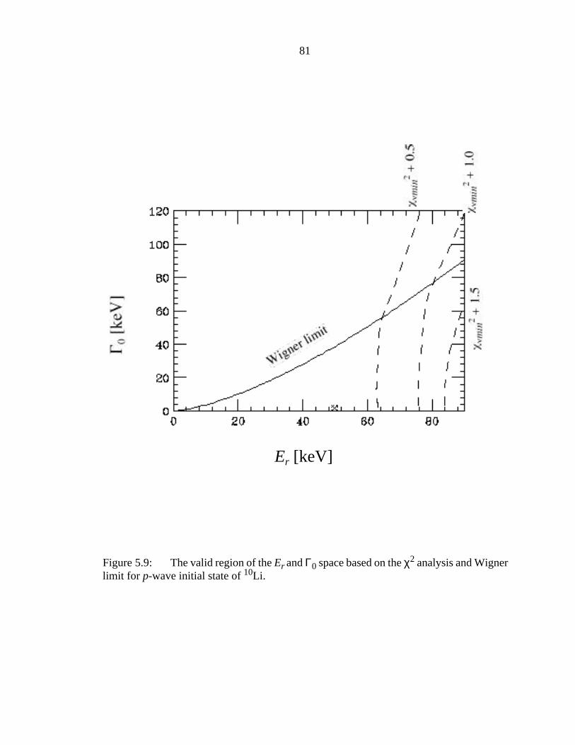
81

Figure 5.9: The valid region of the Er and Γ0 space based on the χ2 analysis and Wignerlimit for p-wave initial state of 10Li.

Er [keV]

82

5.4 The Relative Velocity Spectrum of 13Be

There have been several attempts to measure the ground state of 13Be. Ostrowski et al.

[Ost92] employed the reaction 13C(14C,14O)13Be at ELab = 337 MeV and observed a state

of Sn = -2.01 MeV and Γ0 = 0.32 MeV as the lowest observed state. Penionzhkevich

[Pen94] reported a state at a lower decay energy of 900 keV using the reaction

14C(11B,12N)13Be. The neutron transfer reaction d(12Be,p) was used by Korsheninnikov et

al. [Kor95] and in addition to other excited states the 2 MeV state was observed. Thus, the

state at Er ≈ 2.0 MeV seems to be established, however the existence of the low-lying state

is not confirmed though the existence of an intruder s-wave state at lower energies have

been suggested by theoretical calculations [Len91, Des94, Tho96].

The relative velocity spectrum of the 12Be + n coincidence events is shown in Figure

5.10. The open circles with the error bars show the data and the dotted line indicates the

estimated broad Gaussian background. The spectrum has a single central peak and evidence

of small side peaks around ± 2.0 cm/ns. The simulation for the side peaks was performed

in the same manner as in the 10Li case assuming the d5/2 state of Er = 2.01 MeV and Γ0 =

0.32 MeV [Ost92] of 13Be. The dashed line with two side peaks on the spectrum indicates

the simulated d5/2 state. Since the presence of the d-wave state at Er ≈ 2.0 MeV is in agree-

ment with the previous experiments and the peak positions of the simulation and the small

side peaks of the data matches well, the known d5/2 state was assumed to be in the spectrum

even though the statistics of the data for the side peaks was not sufficient to extract the res-

onance parameters.

Similar to the 10Li case, the central peak in the relative velocity spectrum implies a low-

er energy decay and/or a very wide width of the initial state. It is known that the widths of

83

Figure 5.10: The relative velocity spectrum of the 12Be + n coincidence events.

Vn - Vf [cm/ns]

84

the ground state, the first and the second excited state of the 12Be are narrow [Ajz80]. Thus

the contribution of the final state width to the peak width in the relative velocity spectrum

was negligible compared to the width of the initial state and the width broadening due to

the experimental resolution.

Figure 5.11 shows a level diagram of the decay of 13Be → 12Βe + n. The energy levels

of the 12Be in this diagram were taken from reference [Ajz80]. Two decay scenarios can be

considered to interpret the central peak in the relative velocity spectrum of 13Be. They are

illustrated in Figure 5.11. In case (a) of the figure, the ground state of 12Be is considered to

be the final state of the decay whereas in case (b) the first excited states at Ex = 2.10 MeV

was assumed to be the final state.

In either case, the initial state was assumed to be an s-wave or d-wave since the 13Be

consists of a 12Be core which has a filled p shell [Tho96] for neutrons. The case (a) or (b)

of the decay process, and s or d-wave state as a initial state of the decay were assumed to

extract the decay energy and the width of a 13Be state from the central peak in the 12Be +

n coincidence events. The analysis and the Wigner limit were employed to obtain the

result as in the 10Li case. The individual cases will be discussed in the following sections.

5.4.1 The s-wave Case

Figure 5.12 shows a result of the χ2 analysis if the central peak in the relative velocity spec-

trum was assumed to have a s-wave state as an initial state. The format of the figure is the

same as the 10Li case. The x indicates the reduced chi-square minimum in the decay energy

versus decay width plot. The reduced chi-square minimum position indicates that the state

is at Er = 75 keV and the decay width Γ0 = 110 keV. The limits extracted from Figure 5.12

for the low-lying s-wave state are consistent with theoretical predictions [Ost92, Des94,

χ2

85

Figure 5.11: The level diagram of the possible two cases of the neutron decay of 13Be.

13Be 13Be12Be + n 12Be + n

?

1d5/2

(a) (b)

2.01 MeV2.01 MeV

?2.10 MeV2.71 MeV

4.56 MeV

2.10 MeV2.71 MeV

4.56 MeV

1d5/2

5.13 MeV 5.13 MeV

g.s.g.s.

?

86

Figure 5.12: The valid region of the Er and Γ0 space based on the χ2 analysis and theWigner limit for s-wave initial state of 13Be.

Er [keV]

87

Tho96]. Lenske [Ost92] calculated the low lying s-wave state at Er ≈ 900 keV, whereas

Descouvemont [Des94] predicted a slightly bound s-wave state ar Er = -9 keV or -38 keV.

Thompson and Zhukov [Tho96] calculated s-wave state very close to the threshold with a

scattering length of as ≈ -130 fm (Er < 10 keV). From the constraint of and the

Wigner limit, the maximum possible value for the state of this case is at Er ≈ 1200 keV and

Γ0 ≈ 4400 keV.

The lineshapes of the best fit of the low-lying s-wave state at Er = 75 keV and Γ0 = 110

keV, and the known 5/2+ state at Er = 2010 keV and the width of Γ0 = 320 keV are shown

in Figure 5.13. The relative population of the s-wave and d-wave are 44% and 56%, respec-

tively. Although, the d-state is populated strong, due to the energy dependent efficiency

(see Figure 3.6), it appears substantially weaker in the spectrum. These values are only es-

timates since the efficiency for the decay of the d-wave state is very low.

χνmin2

0.5+

Figure 5.13: The 13Be lineshapes used for the best fit of the simulation to the data. Therelative population of the s-wave and d-wave is 44% and 56%, respectively.

Er [MeV]

s-wave

d-wave

88

Although it can not be ruled out, it is unlikely that the assumed s-wave decays to the

first excited state of 12Be as shown in part (b) of Figure 5.11. It would be dominating decay

to the ground state with a decay energy of ~2200 keV and this would be extremely wide.

Also, the experimental data reported by Ostrowski et al., [Ost92], Penionzhkevich [Pen94],

and Korsheninnikov et al. [Kor95] did not detect any states of 13Be at Er ≈ 2200 keV.

5.4.2 The d-wave Case

The limit of the analysis and the Wigner limit assuming the initial state for the central

peak to be a d-wave state and the final state to be the ground state of 12Be are plotted in

Figure 5.14. The reduced chi-square minimum indicates the decay energy

at Er = 50 keV with essentially a width of 0 keV. As can be seen in Figure 5.14 there is no

experimental limit on the width of the state. However, the decay energy has to be very small

in order to reproduce the central peak and the corresponding Wigner limit makes this an

very unlikely scenario. Such a narrow state should have been observed in the transfer reac-

tions [Ost92, Pen94].

On the other hand, if the case (b) of Figure 5.11 is assumed and the excitation energy

of the 12Be Ex = 2100 keV is taken into account as an offset for the initial state energy level

of 13Be, the overall reduced chi-square minimum is at Er = 2150 keV. Again

the analysis is insensitive with respect to the width. Figure 5.15 shows the χ2 surfaces and

the Wigner limit with the offset of Ex = 2100 keV. Within the uncertainties this would be

consistent with the known d5/2 state in 13Be. The central peak in the relative velocity spec-

trum would then be due to the decay from the tail of the d5/2 state at Er = 2010 keV in 13Be

to the first excited state of 12Be at Er = 2100 keV. Due to the larger decay energy the re-

χ2

χνmin2

1.07=

χνmin2

1.07=

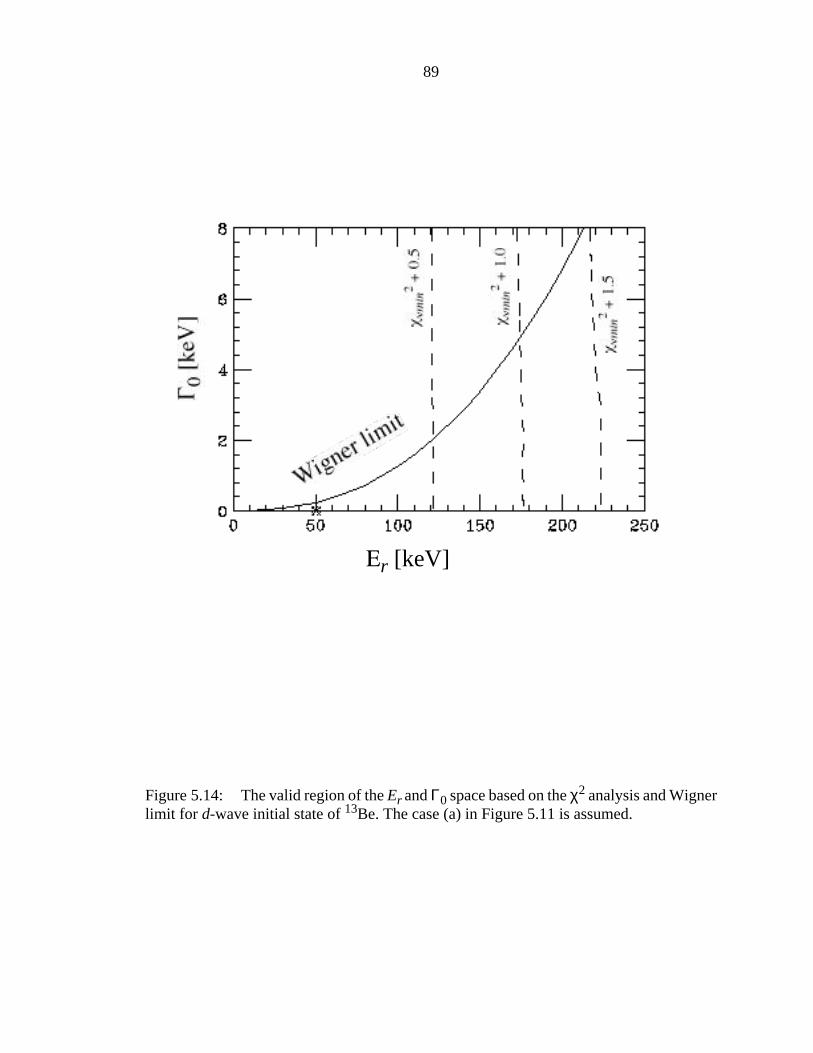
89

r [keV]

Figure 5.14: The valid region of the Er and Γ0 space based on the χ2 analysis and Wignerlimit for d-wave initial state of 13Be. The case (a) in Figure 5.11 is assumed.

90

Figure 5.15: The result of χ2 analysis in the case of d-wave state in 13Be as an initialstate and the first excited state of 12Be as a final state.

Er [keV]

91

striction due to the Wigner limit as in case (a) are not present and the data are consistent

with the measurement of Γ = 300 keV [Ost92]. Thus the scenario is a possible explanation

of the data. The branching ratio for the decay to the first excited state and the ground state

respectively have to be extracted from the shell model calculations, however as explained

in the last section the present data is not very sensitive to the strength distribution.

92

Chapter 6

Summary and Conclusions

The sequential neutron decay spectroscopy (SNDS) at 0˚ was employed to study light nu-

clei beyond the neutron dripline, 10Li and 13Be. The nuclei of interest and the nuclei for the

calibration (7He) were created via fragmentation and decayed immediately to one neutron

and a daughter fragment (9Li, 12Be, and 6He). Neutrons and the daughter fragments were

detected in coincidence and relative velocity spectra were obtained for each isotope from

their information of velocities.

The relative velocity spectra was compared with the spectra created by Monte Carlo

simulations. The simulation code included the decay kinematics, the beam optics, the de-

tector geometry, and the detector efficiencies. The code was tested and adjusted by com-

paring the data of the known decay of 7He and the simulation. Decay parameters of the

observed peaks were extracted with tests.

The result of the 10Li data analysis concluded that the ground state of 10Li is most likely

the low-lying s-wave state. The result obtained suggested the ground state at Er ≈ 50 keV

and Γ0 ≈ 240 keV or in terms of the s-wave scattering length, as ≈ -40.0 fm. It is consistent

with the recent experimental data reported by Zinser et al. [Zin95] and the three-body cal-

culations for 11Li reported by Thompson and Zhukov [Tho94]. The current work experi-

mentally established the existence of the low-lying s-wave ground state of 10Li which was

χ2

93

suggested experimentally by Kryger et al. [Kry93], Young et al. [You94], and Zinzer et al.

[Zin95] and predicted theoretically by Thompson and Zhukov [Tho94]. It is unlikely to im-

prove the experimental limits of the low-lying s-wave ground state in near future due to its

wide width for the low energy level, however the p-wave states at 500 ~ 200 keV observed

by Bohlen et al. [Boh93] and Ostrowski et al. [Ost96] still need to be resolved.

The conclusions from 13Be data showed that there are two possible scenarios for the

observed neutron decay of 13Be. The decay was either from a low-lying s-wave ground

state of 13Be to the ground state of 12Be or from a tail of the known 5/2+ state [Ost92] of

13Be to the first excited state of 12Be. The current result does not distinguish those two cas-

es. One way to resolve these two cases in the future would be to measure γ-rays in coinci-

dence with a neutron and 12Be. If the final state of the decay which caused the central peak

is the first excited state of 12Be, the events would be followed by γ-ray emissions. Further

experimental information of the 13Be ground state is awaited for the understanding of the

neutron dripline nucleus 14Be.

94

BIBLIOGRAPHY

[Ajz80] F. Ajzenberg-Selove and C.L. Busch, Nucl. Phys. A 336, 1 (1980).

[Ajz88] F. Ajzenberg-Selove, Nucl. Phys. A 490, 1 (1988).

[Ame90] A.I. Amelin, M.G. Gornov, Yu.B. Gurov, A.L. Il’in, P.V. Morokhov, V.A.Pechkurov, V.I. Savel’ev, F.M. Sergeev, S.A. Smirnov, B.A. Chernyshev,R.R. Shafigullin, and A.V. Shishkov, Sov. J. Nucl. Phys. 52, 782 (1990).

[Aud93] G. Audi and A.H. Wapstra, Nucl. Phys. A 565, 66 (1993).

[Ban92] J.M. Bang and I.J. Thompson, Phys. Lett. B 279, 201 (1992).

[Bar77] F.C. Barker and G.T. Hickey, J. Phys. G 3, L23 (1977).

[Ber91] G.F. Bertsch and H. Esbensen, Ann. Phys. 209, 327 (1991).

[Bev69] P.R. Bevington, Data Reduction and Error Analysis for the Physical Sci-ences, McGraw-Hill (1969).

[Boh93] H.G. Bohlen, B. Gebauer, M. von Lucke-Petsch, W. von Oertzen, A.N. Os-trowski, M. Wilpert, Th. Wilpert, H. Lenske, D.V. Alezandrov, A.S. Demy-anova, E. Nikolskii, A.A. Korsheninnikov, A.A. Ogloblin, R. Kalpakcheva,Y.E. Penionzhkevich, and S. Piskor, Z. Phys. A 344, 381 (1993).

[Cec79] R.A. Cecil, B.D. Anderson, and R. Madey, Nucl. Instrum. Meth. 161, 439(1979).

[Che70] Y.S. Chen, W.D. Harrison, and T.A. Tombrello, Bull. Am. Phys. Soc. 15,1598 (1970).

[Deá87] F. Deák, A. Kiss, Z. Seres, G. Caskey, A. Galonski and B. Remington, Nucl.Instrum. and Meth. A 258, 67 (1987).

[Des94] P. Descouvemont, Phys. Lett. B 331, 271 (1994).

95

[Esb92] H. Esbensen and G.F. Bertsch, Phys. Rev. C 46, 1552 (1992). See also G.F.Bertsch and H. Esbensen, Ann. Phys. (N. Y.) 209, 327 (1991).

[Fox89] R. Fox, R. Au, and A. VanderMolen, IEEE Trans. on Nucl. Sci. 36, 1562(1989).

[Fox92] R. Fox and J.S. Winfield, NSCL Data acquisition system reference guide,(1992).

[Gol74] A.S. Goldhaber, Phys. Lett. B 53, 306 (1974).

[Gre75] D.E. Greiner, P.J. Lindstron, H.H. Heckman, B. Cork and F.S. Bieser, Phys.Rev. Lett. 35, 152 (1975).

[Han87] P.G. Hansen and B. Jonson, Europhys. Lett. 4, 409 (1987).

[Han95] P.G. Hansen, A.S. Jensen, and B. Jonson, Ann. Rev. Nucl. Part. Sci. 199545, 591 (1995).

[Han96] P.G. Hansen, (private communication).

[Hei90] L.H. Heilbronn, Ph. D. Thesis, unpublished, Michigan State University(1990).

[Hel88] J.H. Heltsley, L. Brandon, A. Galonsky, L. Heilbronn, B.A. Remington, S.Langer, A. Vander Molen, J. Yurkon, and J. Kasagi, Nucl. Instrum. Meth.A 263, 441 (1988).

[Hüf81] J. Hüfner and M.C. Nemes, Phys. Rev. C 23, 2538 (1981).

[Ish96] M. Ishihara, Contribution to the Gull Lake Conference on Nuclear PhysicsNear the Driplines, August 21 - 24, 1996, Gull Lake, Michigan (1996).

[Kno89] G.F. Knoll, Radiation Detection and Measurement, John Willey & Sons,Inc. (1989).

[Kob88] T. Kobayashi, O. Yamakawa, K. Omata, and I. Tanihata, Phys. Rev. Lett.60, 2599 (1988).

[Kob92] T. Kobayashi, Nucl. Phys. A538, 343c (1992).

[Kor95] A.A. Korsheninnikov, E. Yu. Nikolskii, T. Kobayashi, D.V. Aleksandrov,M. Fujimaki, H. Kumagai, A.A. Ogloblin, A. Ozawa, I. Tanihata, Y. Wa-tanabe, and K. Yoshida, Phys. Lett. B 343, 53 (1995).

96

[Kow87] S. Kowalski and H.A. Enge, RAYTRACE manual, Laboratory of NuclearScience and Department of Physics, Massachusetts Institute of Technology,(1987).

[Kra88] Kenneth S. Krane, Introductory Nuclear Physics, John Wiley & Sons(1988).

[Kry93] R.A. Kryger, A. Azhari, A. Galonsky, J.H. Kelley, R. Pfaff, E. Ramakrish-nan, D. Sackett, B. M. Sherrill, M. Thoennessen, J.A. Winger, and S.Yokoyama, Phys. Rev. C 47, R2439 (1993).

[Lan58] A.M. Lane and R.G. Thomas, Rev. Mod. Phys. 30, 257 (1958).

[Lav73] A. Laverne and C. Gignoux, Nucl. Phys. A 203, 597 (1973).

[Len91] H. Lenske, Proc. Int. Symp. on Structure and Reactions of Unstable Nuclei1991, edited by K. Ikeda and Y. Suzuki, World Scientific, Singapore (1991).

[Mig73] A.B. Migdal, Sov. J. Nucl. Phys. 16, 238 (1973).

[Oak92] The formulas and parameters of J.F. Ziegler, The Stopping and Ranges ofIons in Matter, Vols. 3 & 5, Pergamon Press (1980), coded by OakRidgeNational Laboratory, doc. in HHIRF_UBOOK, (1992).

[Orr92] N.A. Orr, N. Anantaraman, Sam M. Austin, C.A. Bertulani, K. Hanold, J.H.Kelley, D.J. Morrissey, B.M. Sherrill, G.A. Souliotis, M. Thoennessen, J.S.Winfield, and J.A. Winger, Phys. Rev. Lett. 69, 2050 (1992).

[Ost92] A.N. Ostrowski, H.G. Bohlen, A.S. Demyanova, B. Gebauer, R. Kalpa-kchieva, Ch. Langner, H. Lenske, M. von Lucke-Petsch, W. von Oertzen,A.A. Ogloblin, Y.E. Penionzhkevich, M. Wilpert, Th. Wilpert, Z. Phys. 343,489 (1992).

[Ost96] A.N. Ostrowski, H.G. Bohlen, B. Gebauer, S.M. Grimes, R. Kalpakchieva,A.A. Korsheninnikov, T.N. Massey, W. von Oertzen, A.A. Ogloblin, Y.E.Penionzhkevich, CH. Seyfert, Th. Stolla, M. Wilpert, and Th. Wilpert, Pro-ceedings of the International Workshop XXIV on Gross Properties of Nu-clei and Nuclear excitations, edited by H. Feldmeier, J. Knoll, and W.Nörenberg, GSI, Germany (1996).

[Pen94] Yu. E. Penionzhkevich, Proc. of the IV. Int. Conf. on Selected Topics In Nu-clear Structure, edited by V.G. Soloviev, Dubna, Russia (1994).

[Pop85] N.A.F.M. Poppelier, L.D. Wood, and P.W.M. Glaudemans, Phys. Lett.157B, 120 (1985).

97

[Rei68] R. Reid, Ann. Phys. 50, 411 (1968).

[Rol88] Rolfs and Rodney, Cauldrons in the Cosmos, The University of ChicagoPress (1988).

[Tal60] I. Talmi and I. Unna, Phys. Rev. Lett. 4, 469 (1960).

[Tan85] I. Tanihata, H. Hamagaki, O. Hashimoto, Y. Shida, N. Yoshikawa, K. Sug-imoto, O. Yamakawa, and T. Kobayashi, Phys. Rev. Lett. 55, 2676 (1985).

[Thi75] C. Thibault, R. Klapisch, C. Rigaud, A.M. Poskanzer, R. Prieels, L. Lessard,and W. Reisdorf, Phys. Rev. C 12, 644 (1975).

[Tho94] I.J. Thompson and M.V. Zhukov, Phys. Rev. C 49, 1904 (1994).

[Tho96] I.J. Thompson and M.V. Zhukov, Phys. Rev. C 53, 708 (1996).

[Tou75] R. de Tourreil and D.W.L. Sprung, Nucle. Phys. A 242, 445 (1975).

[Wap85] A.H. Wapsta, G. Audi, and K. Bos, Nucl. Phys. A 432, 1 (1985).

[Won90] S.S.M. Wong, Introductory Nuclear Physics, Prentice Hall, N.J., USA1990.

[Wou88] J.M. Wouters, R.H. Kraus, Jr., D. J. Viera, G.W. Butler, and K.E.G. Löbner,Z. Phys. A 331, 229 (1988).

[Wil75] K.H. Wilcox, R.B. Weisenmiller, G.J. Wozniak, N.A. Jelley, D. Ashery,and J. Cerny, Phys. Lett. 59B, 142 (1975).

[Win92] J.A. Winger, B.M. Sherrill, and D.J. Morrissey, Nucl. Instrum. Meth. B 70,380 (1992).

[You93] B.M. Young, W. Benenson, M. Fauerbach, J.H. Kelley, R. Pfaff, B.M. Sher-rill, M. Steiner, J.S. Winfield, T. Kubo, M. Hellström, N.A. Orr, J. Steatson,J.A. Winger, and S.J. Yennello, Phys. Rev. Lett. 71, 4124 (1993).

[You94] B.M. Young, W. Benenson, J.H. Kelley, N.A. Orr, R. Pfaff, B.M. Sherrill,M. Steiner, M. Thoennessen, J.S. Winfield, J.A. Winger, S.J. Yennello, andA. Zeller, Phys. Rev. C 49, 279 (1994).

[Vol65] A.B. Volkov, Nucl. Phys. 74, 33 (1965).

98

[Zin95] M. Zinser, F. Humbert, T. Nilsson, W. Schwab, Th. Blaich, M.J.G. Borge,L.V. Chulkov, H. Eickhoff, Th.W. Elze, H. Emling, B. Franzke, H. Freiesle-ben, H. Gissel, K. Grimm, D. Guillemaud-Mueller, P.G. Hansen, R. Holz-mann, H. Irnich, B. Jonson, J.G. Keller, O. Klepper, H. Klinger, J.V. Kratz,R. Kulessa, D. Lambrecht, Y. Leifels, A. Magel, M. Mohar, A.C. Mueller,G. Münzenberg, F. Nickel, G. Nyman, A. Richiter, K. Riisager, C. Sheiden-berger, G. Schrieder, B.M. Sherill, H. Simon, K. Stelzer, J. Stroth, O. Teng-blad, W. Trautmann, E. Wajda, and E. Zude, Phys. Rev. Lett. 75, 1719(1995).