grice on vacuous names - rbjones.com · force new theory "grice"; 3 the problem grice...
TRANSCRIPT

Grice on Vacuous Names
Roger Bishop Jones
Abstract
Formal analysis (using Higher Order Logic with ProofPower) and commentary on Grice’ssystem Q (G, GHP ) first presented in his paper Vacuous Names.
Created 2010/07/07
Last Change Date: 2011/02/02 21:48:21
http://www.rbjones.com/rbjpub/pp/doc/t037.pdf
Id: t037a.tex,v 1.5 2011/02/02 21:48:21 rbj Exp
c© Roger Bishop Jones; Licenced under Gnu LGPL

Contents
1 Prelude 3
2 Introduction 32.1 Background . . . . . . . . . . . . . . . . . . . . . . . . . . . . . . . . . . . . . . . . . . 32.2 Preliminary Formalities . . . . . . . . . . . . . . . . . . . . . . . . . . . . . . . . . . . 4
3 The Problem 4
4 System Q: Objectives 5
5 Classical Logic using HOL 65.1 Scope . . . . . . . . . . . . . . . . . . . . . . . . . . . . . . . . . . . . . . . . . . . . . 65.2 Semantic Domains . . . . . . . . . . . . . . . . . . . . . . . . . . . . . . . . . . . . . . 7
5.2.1 Interpretations . . . . . . . . . . . . . . . . . . . . . . . . . . . . . . . . . . . . 85.3 Descriptions . . . . . . . . . . . . . . . . . . . . . . . . . . . . . . . . . . . . . . . . . . 95.4 Propositional Logic . . . . . . . . . . . . . . . . . . . . . . . . . . . . . . . . . . . . . . 95.5 Quantifier Inference-Rules . . . . . . . . . . . . . . . . . . . . . . . . . . . . . . . . . . 105.6 P Committal . . . . . . . . . . . . . . . . . . . . . . . . . . . . . . . . . . . . . . . . . 10
6 System C 116.1 Quantifier Inference-Rules . . . . . . . . . . . . . . . . . . . . . . . . . . . . . . . . . . 146.2 Existence . . . . . . . . . . . . . . . . . . . . . . . . . . . . . . . . . . . . . . . . . . . 14
6.2.1 A. (E Committal) . . . . . . . . . . . . . . . . . . . . . . . . . . . . . . . . . . 146.2.2 B. Existentially Quantified Formulae . . . . . . . . . . . . . . . . . . . . . . . . 15
6.3 Identity . . . . . . . . . . . . . . . . . . . . . . . . . . . . . . . . . . . . . . . . . . . . 156.4 Names and Descriptions . . . . . . . . . . . . . . . . . . . . . . . . . . . . . . . . . . . 16
7 System S 177.1 Quantifier Definitions . . . . . . . . . . . . . . . . . . . . . . . . . . . . . . . . . . . . 217.2 Quantifier Inference-Rules . . . . . . . . . . . . . . . . . . . . . . . . . . . . . . . . . . 227.3 Existence . . . . . . . . . . . . . . . . . . . . . . . . . . . . . . . . . . . . . . . . . . . 22
7.3.1 A. (E Committal) . . . . . . . . . . . . . . . . . . . . . . . . . . . . . . . . . . 227.3.2 B. Existentially Quantified Formulae . . . . . . . . . . . . . . . . . . . . . . . . 23
7.4 Identity . . . . . . . . . . . . . . . . . . . . . . . . . . . . . . . . . . . . . . . . . . . . 23
8 Conclusions 24
9 Postscript 24
A Theory Listings 25A.1 The Theory grice . . . . . . . . . . . . . . . . . . . . . . . . . . . . . . . . . . . . . . 25A.2 The Theory griceC . . . . . . . . . . . . . . . . . . . . . . . . . . . . . . . . . . . . . 27A.3 The Theory griceS . . . . . . . . . . . . . . . . . . . . . . . . . . . . . . . . . . . . . . 29A.4 * . . . . . . . . . . . . . . . . . . . . . . . . . . . . . . . . . . . . . . . . . . . . . . . . 31
Bibliography 31A.5 * . . . . . . . . . . . . . . . . . . . . . . . . . . . . . . . . . . . . . . . . . . . . . . . . 32
Index 32
2

1 Prelude
This document is intended possibly to form a chapter of Analyses of Analysis [7].
My initial purpose in preparing the document is simply to investigate and analyse Grice’s “SystemQ” (since renamed “System G” by Myro and “System GHP ” by Speranza) using a decent proof tool.
Further discussion of what might become of this document in the future may be found in my postscript(Section 9).
In this document, phrases in coloured text are hyperlinks, like on a web page, which will usually getyou to another part of this document (the blue parts, the contents list, page numbers in the Index)but sometimes take you (the red bits) somewhere altogether different (if you happen to be online)like the hist-analytic archives.
For description of the formal languages, methods and tools used in or in producing this documentsee: [6].
2 Introduction
I will endeavour to follow the structure of Grice’s paper Vacuous names[4, 2]. However, the methodemployed for the formal analysis, which is called “shallow embedding”, is essentially semantic, andinvolves addressing semantic fundamentals before finding manageable syntactic presentations, and Itherefore find it necessary to address key aspects of the semantics before considering the details ofsyntax.
2.1 Background
Grice’s deliberations about Vacuous Names may be understood primarily against those who havesupposed or desired a significant difference between formal logics and the logic of ordinary discourse,by one who felt that the differences are, or need only be, modest. In some of his writings. forexample in the “Retrospective Epilogue” in Sudies in the Way of Words[5], Grice describes twocamps, “Modernists” and “Neo-traditionalists”, the former making more and the latter less of thedistinctions between formal and ordinary logic.
Elsewhere in Grice’s philosophy, in connection with this controversy, the relationship between thelogical connectives and their ordinary language counterparts is discussed. Here we are concernedwith the problem of referring expressions which lack a referent.
Modern discussion of this problem begins with Russell [10, 11], who sought formal languages formathematics which were more precise and more transparent in their logical structure than is ordinarylanguage.
There are two aspects of the problems here at stake which are separable. One concerns logic andlanguage; how we talk and reason using words or phrases which do not, or might not, refer to anyexistent entity. The second is the metaphysical question of what exists. Russell’s most importantwork in this area arose from his making a transition away from a lavish Meinongian ontology inwhich there are different kinds or grades of existence, to the adoption of Occam’s razor, leading to aspartan ontology. Key to this is the acceptance that some referring phrases fail to refer, and Russell’sprincipal contribution here is in his theory of descriptions [11, 10].
Russell’s theory treats definite and indefinite descriptions as “incomplete symbols”, which contributeto the meaning of the sentence as a whole even if they fail to refer. Such incomplete symbols are
3

only meaningful in certain particular context, and their meaning is given by translated the wholeinto some other phrase in which the incomplete symbol does not occur and in which there remainsno explicit reference to an entity which might not exist. Usually this involves quantification. Propernames are then eliminated in favour of descriptions.
Grice’s principal aim is to resurrect the conception of names as references, rather than as surrogatesfor descriptions. He wants to do this without being forced to regard names of non-existent entities,such as Pegasus, as yielding sentences which are neither true nor false. This he achieves by allowingthat names which do not designate nevertheless refer to some kind of entity which he calls itscorrelate, and by the rule that predications to non-designating names are to yield falsehoods.
2.2 Preliminary Formalities
I consider two different approaches, both derived from Grice, to the problems discussed in VacuousNames[4]. Much of the discussion concerns matters which are common to both, and this involvessome formal material. In order to avoid replication the formalisation of this common ground isprovided first in a separate theory before matters specific to the two variants are entered into.
Common material is in the theory ‘grice’ whose listing may be found in appendix A.
SML
open theory "rbjmisc";
force new theory "grice";
3 The Problem
Grice uses several lists in his presentation. To simplify unambiguous reference I have prefixed someof the numbering schemes with capital letters.
Our starting point is a list of eight inclinations supplied by Grice and summarised here:
I1 That individual constants be admitted.
I2 Note that names are sometimes “vacuous”
I3 Thence that a constant might lack a designatum.
I4 That excluded middle and bi-valence nevertheless remain unqualified.
I5 That a claim about (predication to) a non-designating constant be false and its negation true.
I6 That no unusual constraints on “U.I.” 1 and “E.G.” 2 be introduced.
I7 That the law of identity (in the form @x x � x) be a theorem3.
I8 That derivability implies entailment.4
In relation to these Grice points out two difficulties as follows:
1Universal Instantiation2Existential Generalisation3Which seems to suggest that identity is not a predicate.4i.e. that the system be sound!
4

(a) I2, I3 and I7 between them seem prima facie to enable proofs of the existence of non-existententities (e.g. “Pegasus exists”).
(b) I5 and I6 would if gratified permit us to infer that there exists something which does not flyfrom the premise that Pegasus does not exist.
He then lists five possible resolutions the difficulties:
R1 To resist I3 and insist that constants have a designatum.
R2 Resisting I4 and I5, insist that predications to non designating terms and their negations lacka truth value.
R3 Resist I1 and do without individual constants.
R4 Resist I2 by insisting that all constants have a designatum, which might perhaps “be” withoutexisting.
R5 Resist I6 by adding requirements on existential generalisation that the relevant constant beshown to designate.
R6 Resist I8, allowing that the deductive system be not strictly sound, but only so subject to thecondition (or “marginal” assumption) that all names have bearers.
Grice does not discuss any of these alternatives, but instead proposes to attempt to square the circleby devising a system which satisfies all these (apparently) incompatible inclinations.
4 System Q: Objectives
Grice now proposes a first order predicate calculus meeting two particular objectives, spelt out infive points of further detail.
(i) That a sentence such as “Pegasus does not fly” be capable of rendition in two distinct waysone of which will be true and the other false in the case that Pegasus does not exist. Thesecorrespond to disambiguations of the logical structure of the sentence either as predicatingnon-flying or denying a predication as flying.
(ii) That in either case the inference from “Pegasus does not fly” to “there is something which doesnot fly” is to be admitted.
O1 U.I. and E.G. are acceptable without special side conditions.
O2 Some sentences involving non-denoting constants will be true and provable.
O3 It will be formally decidable whether a sentence depends for its truth on whether some constantdesignates.
O4 It will be possible to find in Q representation of sentences such as “Pegasus exists”.
O5 There will be an extension of Q in which identity is represented.5
5No discussion here of whether identity is a predicate.
5

5 Classical Logic using HOL
Grice tries to make his system as close as possible to “classical logic”, basing his system on a firstorder predicate calculus presented as a natural deduction system based on a textbook by Mates [8].I hope that the pertinent sense of “classical” here is two-valued.
In this presentation we work with a “classical” higher order logic (based on Church’s formulation ofthe Simple Theory of Types[1]) in the form of a sequent calculus. In this section we replicate in thissystem theorems which show the closeness of the relationship between this classical logic and the onefrom which Grice departs.
Grice discusses the problem of the scope of names before getting into the details of his classical logic,but since we here adopt a different manner of resolving this problem which depends upon specialfeatures of our “classical logic”, the discussion of scope belongs here.
5.1 Scope
A part of the novelty and difficulty in system Q lies in its special provisions for controlling the“scope” of names.
The use of the word scope in this context is distinct from its more common usage (at least inmathematical logic and computer science) in which the (or a) scope of a name (variable or constant)is a syntactic region within which it may be used with the same sense (as opposed to uses of thesame name for entirely distinct purposes as may appear in different scopes of the name).
In this case the relevant ambiguity of scope is not a region of significance of the name, but the extentof some predicate applied to the name. Thus in the example used by Grice, there is an ambiguity inthe sentence “Pegasus does not fly” about the logical structure of the sentence which leaves doubtabout what predicate is being applied to Pegasus. We may regard the sentences as predicating “xdoes not fly” of Pegasus, or we may be denying that the predicate “flies” applies to Pegasus. Thequestion is whether the negation is part of the predicate or is applied to the result of the predication.
In System Q Grice provides a predicate logic in which numerical subscripts may be used to disam-biguate the predications which are taking place. Unfortunately, this notation, like the dot notationin Principia Mathematica is not as readable as the more usual use of brackets for disambiguatingscope. Furthermore, this aspect of the syntax would be hard to replicate by the methods we proposeto adopt, which are intended to permit a lightweight analysis of semantic issues and their connectionwith the validity of sentences and the soundness of derivations.
In our analysis we will therefore provide for the desired control over predication by the use of Church’slambda notation. We expect that our syntax will be readily related to that of System Q, but sincethe system we formalise is at least syntactically distinct we will call it system C6.
System C is obtained by conservative extension to HOL, which is a version of higher order logicderived directly from Church’s Simple Theory of Types [1]. Church’s STT is distinctive for itsvery slender logical core, achieved by building the logical system from the simply typed lambdacalculus. In this logical system boolean valued functions serve for predication, and the ideas of Griceon vacuous names are realised principally by defining a different kind of predication. To minimiseconfusion, the word predicate will only be used when Grice’s notion of predication is intended,otherwise propositional or boolean valued function will be used.
The use of lambda notation for making explicit the predicate to be applied may be illustrated simply
6This in homage to Rudolf Carnap, Q having been chosen by Grice in homage to Quine, and G having been chosenby Myro[3, 9] in homage to Grice.
6

using Grice’s Pegasus example. In using this method we must distinguish two kinds of predication.The kind whose scope we are now discussing, which is the only kind of predication in System Q, andthe kind of predication which we have in HOL, consisting in the application of a propositional functionto some argument. Henceforth these two will be distinguished by using the term “predication” onlyfor the former, by making this kind of predication explicit in the concrete syntax as a copula, and byusing the phrase “application of a propositional function” for the second kind of predication. Theuse of a copula not only visually distinguishes Griceian predication, but also allows us to control itssemantics through the definition of the copula.
The copula will be the word “is”, and since we will be discussion more than one variant of Grice’ssystem, the copulas will be distinguished by subscripts giving the name of the system to which theybelong. In System C, then, the copula is “isc”, so the application of the predicate “Flier” to theterm “Pegasus” will be written “Pegasus isc Flier”.
The two variants of “Pegasus does not fly” are then expressed as:
“ pPegasus isc Flierq ”
and
“Pegasus isc pλx Flier x q”.
In the first case the predicate applied to Pegasus is pFlier q , in the second case it is pλx Flier xq(which is a negation of Flier, “not a flier”).
This technique makes it possible to examine the semantic aspects of System Q using formal machineassisted deductive reasoning, while avoiding the special intricacies of formalising Grice’s specialsyntax. Whether this pays off in terms of perspicuity and penetration in the analysis remains to beseen.
We will therefore offer no further discussion of Grices notational devices for scoping at this point,but may consider later how much may have been lost by this approach.
At this stage I am looking at two alternatives for the underpining semantics, and the following twosection work through these two alternatives. In each case, we are devising a “shallow embedding” ofsomething close to Grice’s System Q in ProofPower HOL. These embedded aproximations to SystemQ are called System C (in homage to Rudolf Carnap) and System S (a nod to Speranza).
5.2 Semantic Domains
Grice goes on from his discussions of scope to the presentation of the remaining aspects of the syntax,notably of the various aspects of the deductive system.
We will track this discussion of inference in a semantic way, demonstrating the semantic principleswhich ensure the soundness of the deductive system presented in a manner which makes reasonablyclear the relationship between the two. This amounts to a semantic embedding into HOL of a systemwhich is intended to be semantically parallel to system Q, though not syntactically quite the same.
To do this we must first provide some basic definitions on which the semantics is based, and beforedoing that I must explain part of the method of semantic embedding which might seem to, butdoes not in fact, prejudice one of the principle issues at stake. That is that the embedding consistsin a development of a semantics which is purely denotational, i.e. in which every expression has adenotatum. These denotation need not be what one would naturally suppose the reference of anexpression to be, they may be purely abstract surrogates which suffice to describe the truth conditionsof the language. So the way we model a language in which term expressions may not denote, is by
7

taking the range of things which they might possibly denote, and adding one or more extra itemswhich are values which they are give to indicate that they have no denotation.
5.2.1 Interpretations
Grice’s definition of an interpretation of Q (VIII A of [4]) is ambiguous in what it says about thedomain of an interpretation. The domain is a set of correlates, some of which may be unit sets theelement of which is a designatum. Grice tells us that there need not be any such unit sets, but doesnot say explicitly that there may be no other correlates. He does tell us that he has in mind thatthere will be exactly one non-designating correlate, the empty set, but he does not place this as arequirement, so the significance of his having this in mind is unclear.
There are three possibilities concerning the number of non-designating correlates in an interpretation,that there are none, exactly one, or more than one. In relation to these there are a number of possiblepositions in relation to the definition of an interpretation, the most obvious are:
1. no constraint
2. there must be at least one
3. there must be exactly one
Of course there may be more, but I propose to discuss just these three.
From a literal reading of Grice in this section I would take the first. However, from the fact thathe explicitly allows there to be no designata but does not explicitly say this for non-designatingcorrelates, we might infer that he intends but does not state that there will be at least one non-designating correlate. Alternatively we might take the case he had in mind more presciptively andwork with item 3.
These are significant semantically, of course.
Allowing interpretations with no designata will create problems with descriptions if these were to beintroduced into Q, for one would then have no correlate available for a non-designating descriptions.It also affects a matter which Grice later discusses, which is whether certain existential claimsare valid, notably the claim that there is something which does not exist. This (or somethingsimilar “ Dx 4 . 3 F 1 x 2
2”, VIII B p137) Grice later claims to be valid, and this is evidence againstinterpretation 1 in favour of 2 or 3.
Item 2, though the one perhaps preferred by Grice, has the disadvantage that all non-designatingterms have the same correlate, and will therefore be equal in a sense of equality which satisfies theuniversal law of reflexivity of identity. Do we want Pegasus and Sherlock Holmes to be identical?
Nevertheless, in our shallow embedding of Q we will adopt 2, for, in addition to its possible prefermentby Grice, and its confirming Grice’s belief in the validity of the cited existentials, it allows a simplerand more transparent shallow embedding than either of the others. [fuller explanation to be supplied]
First let us give a name for the domain of discourse of an interpretation of the language Q. Wewill suppose this to be a “type” in HOL, but will leave open the type by using a type variable. Toserve as denotions for terms in system GHP we use a disjoint union of two types, the first of which isthe type of those things which do exist (candidate designata) and the second is a type of surrogates(“correllates” in Grice) for those things which do not exist. We use V for Value.
8

5.3 Descriptions
When Grice comes to discuss descriptions he has in mind a distinction between descriptions andnames which would impact upon the kind of interpretation necessary for a semantic embedding.This in turn would impact the detailed definition of the copula.
To make apparent the differences which would arise in treating descriptions as Grice intends weprovide two treatments of those aspects of the logical system which depend upon the details of thesemantics. These will be called System C and System S.
Certain aspects of our presentation, particularly those which simply illustrate the correspondencebetween the classical propositional logic in System Q and that in ProofPower-HOL, are common toSystem C and System S and are therefore treated first.
5.4 Propositional Logic
The following material is common to Systems C and S and shows how these systems relate to thepropositional logic in System Q. Since we are working with a semantic embedding rather than asyntactic meta-theory we cannot prove results about derivations and instead present proofs aboutthe semantics which show that the required inference rules would be sound.
To do this we adopt a notation for expressing entailment in C in a manner parallel to the presentationof the natural deduction system of Q. This is done by defining the infix relationship pal |ù cq holdingbetween a list of assumptions (or premises) al and a single conclusion c when the conclusion is entailedby the premises.
SML
declare infix p4 , "|ù"q;
HOL Constant
$|ù : BOOL LIST Ñ BOOL Ñ BOOL
@al c pal |ù cq ô p@L alq ñ c
In the following theorems which capture the content of Grices rules for Q as theorems of C, thevariables φ, ψ, ζ... range over formulae (boolean terms) and Γ, ∆, Θ... over lists (finite sequences) offormulae. P ranges over propositional functions, values whose types are instances of p :’a Ñ BOOLq(in which 1a is a type variable). The notation “[φ; ψ; ...]” is an explicit list formation (“[φ]” being a
single element list) and the symbol “a” is the concatenation operator over lists.
In general the rules of Q can be formulated as theorems of HOL because in a higher order logic,and can quantify over predicates. This means that where substitution is involved in a rule, this iscaptured as a theorem by the use of a variable as a predicate applied to a variable as an argument.When such a theorem is instantiated using a lambda expression as the predicate, the substitutioninto the expression will be achieved by beta-reduction.
9

ASS � $ @ φ rφs |ù φ
RAA � $ @φ ψ ζ Γ prφs a Γ |ù ψ ^ ψq ñ pΓ |ù φq
DN � $ @ φ r φs |ù φ
^I � $ @ φ ψ rφ; ψs |ù φ ^ ψ
^E � $ @ φ ψ prφ ^ ψs |ù φq ^ prφ ^ ψs |ù ψq
_I � $ @ φ ψ prφs |ù φ _ ψq ^ prφs |ù ψ _ φq
_E � $ @ φ ψ ζ Γ ∆ Θ prφs a Γ |ù ζq ^ prψs a ∆ |ù ζq ^ pΘ |ù φ _ ψq
ñ pΓ a ∆ a Θ |ù ζq
CP � $ @ φ ψ Γ prφs a Γ |ù ψq ñ pΓ |ù φ ñ ψq
MPP � $ @ φ ψ rφ ñ ψ; φs |ù ψ
5.5 Quantifier Inference-Rules
We now show the correspondence between the quantification rule in System Q with the standardquantifiers in HOL. Because of this correspondence we can use the standard HOL quantifiers inSystem C and get a good correspondence with System Q in this area. When we come to System Sit will be necessary to redefine the quantifiers to obtain those qualifications on @E and DI which arenecessary to cope with Grice’s ideas about failing descriptions.
@I � $ @ Γ P p@ x Γ |ù P x q ñ pΓ |ù p@ x P x qq
@E � $ @ Γ P c pΓ |ù p@ x P x qq ñ pΓ |ù P cq
DI � $ @ Γ P x pΓ |ù P x q ñ pΓ |ù pD x P x qq
DE � $ @ P Q p@ x rP x s |ù Qq ñ prD x P x s |ù Qq
5.6 P Committal
The notion of E-committal is defined syntactically by Grice, and tells us which formulae in SystemQ are true only if some name has a designatum, i.e. to the existence of which named individuals ourassertion of the formula would commit us.
In HOL we can formalise this idea without resort to reasoning about syntax, furthermore, the maindetail in the definition is independent of whether we are in System C or System S, and is thereforeprovided here. To achieve this we parameterise the definition of E-committal so that it can bespecialised to the different ways of asserting existence in Systems C and S, the parameterised versionbeing called P committal.
The formal criteria for E committal then becomes provability in HOL (which is not in generaldecidable).
In Grice E committal is a relationship, here it is a parameterised property of propositional functions(the parameter being the relevant notion of existence).SML
declare infix p100 , "committal"q;
HOL Constant
$committal : p1a Ñ BOOLq Ñ p1a Ñ BOOLq Ñ BOOL
@P φ P committal φ ô @α φ α ñ P α
10

The following theorems correspond to clauses in Grice’s definition of E committal :
P 2 � $ @ P φ P committal φ
ñ P committal pλα φ αq
P 3 � $ @ P φ ψ P committal φ _ P committal ψ
ñ P committal pλ α φ α ^ ψ αq
P 4 � $ @ P φ ψ P committal φ ^ P committal ψ
ñ P committal pλ α φ α _ ψ αq
P 5 � $ @ P φ ψ P committal pλ α φ αq ^ P committal ψ
ñ P committal pλ α φ α ñ ψ αq
P 6@ � $ @ P φ pD β P committal pφ βqq
ñ P committal pλ α @ β φ β αq
I have a problem proving the existential element of (6), so this clause is in doubt. I think Griceshould be asking for “@β ψpβ{ωq” to be E committal for α (in system Q), which corresponds insystems C and S to the theorem:
P 6Db � $ @ P φ p@ β P committal pφ βqq
ñ P committal pλ α D β φ β αq
(with P suitably instantiated).
6 System C
A new theory is needed which I will call “griceC” which is created here:
SML
open theory "grice";
force new theory "griceC";
set pc "rbjmisc";
Grice introduces a special notion of interpretation in terms of which to give the semantics of Q. Aninterpretation has a domain which is a set of correlates, some of which are unit sets, in which case themember of that unit set is called a designatum. For uniformity of type we assume that all correlatesare sets of sets.
We allow the domain of an interpretation to be any type and for some element of that type to beidentified as THE non-designating element.
HOL Constant
K: 1a
T
We can then use inequality with K as the property of being a designatum. The structure of theseinterpretations is isomorphic to that of Grice’s preferred notion of interpretation, even though we donot use unit sets for correlates of designating constants.
We may use HOL constants of appropriate type for Q constants and predicates, and HOL variablesfor Q variables, and the consequence should be that the theorems provable in HOL should be justthose which are valid in Q.
11

This is done by using T and F instead of Corr(1) and Corr(0) respectively.
Now we define our special kind of predication. This is done by introducing ‘is’ subscripted with ‘c’as a copula.
SML
declare infix p400 , "isc"q;
HOL Constant
$isc : 1a Ñ p1a Ñ BOOLq Ñ BOOL
@ p t t isc p ô if t � K then F else p t
The definition says, if the term denotes then apply the predicate to the value denoted, otherwise theresult of the predication is F (false).
Note that this will not work for relations, we would have to define a separate similar predicator foreach arity of relation in use.
Here is the copula for applying a 2-ary relation.
SML
declare infix p400 , "isc2"q;
HOL Constant
$isc2 : p1a � 1bq Ñ p1a � 1b Ñ BOOLq Ñ BOOL
@ p t t isc2 p ô if Fst t � K _ Snd t � K then F else p t
Now let’s introduce Pegasus. The “definition” just says that Pegasus is the non-denoting value.
HOL Constant
Pegasus : 1a
Pegasus � K
And the predicate Flier. Note that the predicates apply only to real desigata under the normalHOL application, its only under our special predication that they become applicatble to possiblynon denoting values.
HOL Constant
F lier : 1a Ñ BOOL
T
We can now prove in HOL the elementary facts we know about Pegasus flying, yielding the followingtheorems:
12

Pegasus lemma 1 �
$ Pegasus isc Flier ô F
Pegasus lemma 2 �
$ Pegasus isc pλ x Flier x q ô F
Pegasus lemma 3 �
$ Pegasus isc Flier
Pegasus lemma 4 �
$ Pegasus isc pλ x Flier x q
In case you may doubt the neutrality of our use of lambda expressions, we show here that theyare inessential to this approach, and can be dispensed with in favour of explict definitions of thepredicates required. Thus we may instead define a predicate which is the denial of Flier :HOL Constant
NonF lier : 1a Ñ BOOL
@x NonFlier x ô Flier x
We can then prove the slightly reworded:
Pegasus lemma 5 � $ Pegasus isc NonFlier ô F
the proof of which need not mention the predicate, since it suffices to know that the subject doesnot exist.
This general claim can be expressed in HOL and proven. To make it read sensibly however, it is bestfor us to define the relevant notion of existence.HOL Constant
Existent : 1a Ñ BOOL
@x Existent x ô T
The definition looks a bit bizarre and works for just the same reason that we do not need to knowthe predicate to know that predication to a non-existent will be false. This predicate will always betrue, unless it is applied to a term which fails to denote. So we satisfy another of Grice’s desiderata,that the non-existence of Pegasus can be stated.
But first a more general result:
Existent lemma 1 �
$ @ P x x isc Existent ñ x isc P
Desideratum A8 is satisfied by the standard quantifiers in HOL.
D lemma 1 �
$ @ P Pegasus isc P ñ pD x x isc Pq
@ lemma 1 �
$ @ P p@ x x isc Pq ñ Pegasus isc P
13

6.1 Quantifier Inference-Rules
An example of the effect of substitutions obtained by use of these theorems in C intended to mimicthe rules of Q is as follows.
Take ths simple case of @E, with the predicate λx x isc Flier , which we seek to instantiate toPegasus.
We can specialise @E to this case like this:
SML
val sve � list @ elim rprs:BOOL LISTq, pλx x isc Flierq, pPegasusqs @E ;
This gives the theorem:
val sve � $ prs |ù p@ x pλ x x isc Flierq x qq
ñ prs |ù pλ x x isc Flierq Pegasusq : THM
in which there are two occurrences of the lambda expression in the places previously occupied bythe variable P .
The substitutions can then be effected by beta reduction which can be achieved by rewriting thetheorem as follows:SML
rewrite rule rs sve;
Which yields a theorem justifying the required inference.
val it � $ prs |ù p@ x x isc Flierqq ñ prs |ù Pegasus isc Flierq : THM
All the above rules simply explicate the standard aspects of the logic of Q and C and do not reflectthe specific additional features which Grice requires in connection with vacuous names. They simplyillustrate that the logical context for C includes as much standard logic as is provided in Q, andprovide some tenuous indication that Grice’s rules conform to standard logic as defined in Church’ssimple theory of types. The main risk for Grice is in the detail of his presentation, bearing in mindthe additional complexities arising from his suffix notation, and the above exercise offers no assurancein that matter.
6.2 Existence
6.2.1 A. (E Committal)
We have already defined the predicate “Existent” which tells us whether a name designates.
The following theorem indicates that the propositional function captures the intent of Grice’s “+ex-ists” notation.
E1 �$ @φ α α isc φ ñ α isc Existent
E Committal Grice’s notion of E committal corresponds in System C to the previously definedgeneric notion of committal instantiated to the propositional function Existent.
The definition we have already given for Existent is similar in character and identical in effect toGrices suggestions for +exists.
14

6.2.2 B. Existentially Quantified Formulae
This has already been covered.
Grice wishes to distinguish himself from Meinong, but his system allows quantification over non-existents, and he can therefore only distinguish himself from Meinong by distancing himself alsofrom Quine’s criterion of ontological committment. This he could easily do by adopting Carnap’sdistinction between internal and external questions, and denying that any metaphysical significanceattaches to something being counted in the range of quantification.
6.3 Identity
HOL already has identity and this identity is good for System C. In HOL identity is a curriedpropositional function of polymorphic type p :’aÑ ’aÑ BOOLq. If applied using function applicationthe universal law of reflexivity holds.
To get a “strict” version of equality (i.e. one which is false when either argument does not exist) itis necessary to uncurry equality so that its type becomes p :(’a � ’a) Ñ BOOLq and apply it usingthe system C copula for binary relations.
These two seem to correspond to Grice’s intended two kinds of equality, insofar as the differencebetween the two is primarily that one does and the other does not allow that there may be trueidentities between non-denoting names. However this is achieved in system C by having two quitedistinct identity relations only one of which is properly a predicate, and applied through our copulaisc. The other is a propositional function which must be applied without use of the copula (becausethe copula forces strictness, i.e. forces predication to undefined values to yield falsehoods).
Grice seems to think that the required distinction between equalities can be achieved by the use ofhis scoping subscripts, but I have not yet been convinced that he is correct in this. Whatever thescope of the predicate, predication to non-denoting names must yield falsehood, so I can’t see howany use of subscripts will make “Pegasus = Pegasus” to be true.
To illustrate the effect of the built-in equality the following theorems suffice:
Pegasus eq lemma1 �
$ Pegasus � Pegasus
Note the lack of copula. This is of course an instance of the theorem:
eq refl thm �
$ @ x x � x
To get a nice notation for “strong” equality we need to define it as an infix symbol, which requiresthat the copula be built into the definition. We could use the � symbol, but this usually represents anequivalence relation which is weaker than identity, so we will subscript the � sign with c, suggestingthat it is just the same thing applied through our copula.SML
declare infix p200 , "�c"q;
HOL Constant
$�c : 1a Ñ 1a Ñ BOOL
@x y :1a px �c yq � px ,yq isc2 pUncurry $�q
15

We can now prove:
Pegasus eq lemma2 �
$ Pegasus �c Pegasus
And must rest content with the qualified rule:
eqc refl thm �
$ @ x x isc Existent ô x �c x
The “strictness” of this equality is expressed by the theorem (which would have made a betterdefinition):
eqc strict thm �
$ @ x y x �c y ô x isc Existent ^ y isc Existent ^ x � y
On reflection Grice’s treatment by scoping is presented in the context of a second order definition ofequality, and therefore for the weak equality does not define equality as a predicate, but as a secondorder formula. Its equivalence to the primitive equality in HOL can be illustrated by the followingtheorem:
snd order eq thm �
$ @ x y x � y ô p@ P x isc P ô y isc Pq
This equivalence only holds because we adopted Grice’s preferred (but not stipulated) domain ofinterpretation, in which there is exactly one non-designating correlate. If there was more thanone non-designating correlate then Grice’s second order definition would give a notion of identityunder which all non-designating correlates are considered equal, which would not be the case for theprimitive equality in HOL.
Even in that case a similar device would work as illuatrated by the following theorem:
snd order eq thm2 �
$ @ x y x � y ô p@ P P x ô P yq
In which the griceian copula has been dropped so that the predication is no longer strict.
6.4 Names and Descriptions
I note here pro-tem just that the method adopted in System C for controlling the scope of predi-cations, viz. the use either of lambda expressions or of naming complex predicates by definitions,enables scope to be controlled in predication to descriptions which are formed as terms. We cantherefore follow Grice’s system Q in introducing such descriptions.
SML
declare binder "ι";
HOL Constant
$ι : p1a Ñ BOOLq Ñ 1a
@φ p$ι φq � εα pα isc φ ^ @β β isc φ ñ β � αq
_ p Dγ γ isc φ ^ @β β isc φ ñ β � γq ^ α � K
16

ι thm1 � $ @ γ γ isc φ ^ p@ β β isc φ ñ β � γq ñ $ι φ � γ
ι thm2 � $ pD γ γ isc φ ^ p@ β β isc φ ñ β � γqq ñ $ι φ � K
There is a difficulty in adopting Grice’s reticence to allow existential generalisation on the basisof such a predication. This cannot be supported in system C without changing the underlyingsemantics.
Grice has effectively split the non-denoting expressions into two, those which correlate with somethingin the domain of quantification and those which do not. Since our embedding requires all expressionsto have a value, we would have to add another kind of entity into the domain of interpretation anddefine quantifiers which operate over expressions which have a correlate but not over the values ofnon-denoting descriptions.
This would effect most of the embedding, the whole would have to be reworked (in a routine way).We investigate this possibility in the next section.
7 System S
System S contains two minor adjustments to System C which are concerned with the treatment ofnon-designating names and failing descriptions. In relation to non-designating names, the semanticsin System S now allows that they have distinct correlates. In addition a new subdomain is introducedwhich provides at least one (since we can always prove that there is a failing description) surrogatefor a failing description. The primary reason for recognising, in the semantics, denotations for failingdescriptions, is so that we can arrange as Grice seems to require, that they do not fall into the rangeof the System S quantifiers. This in turn results in the qualification of the rules EG and UI.
A new theory is needed which I will call “griceS” which is created here:
SML
open theory "grice";
force new theory "griceS";
set pc "rbjmisc";
We liberalise the notion of interpretation from system C in the following two ways. Firstly we allowthat there may me more than one non-denoting correllate. and hence then there may be semanticdistinctions between non-denoting names, overcoming one obstacle to substantial discussions aboutfictional entities. Secondly we introduce values to stand for non-referring descriptions. These arenot intended to be values and will be excluded from the range of quantification, with the effect thatEG and UI will not work with failing descriptions.
This will be done using a “disjoint union” the right disjunct of which will be surrogates for failingdescriptions, and the left will be correlates for names of which there will be at least one which is nota denotatum. The “normal” quantifiers for system S will quantify only over the correlates.
To effect this we introduce the property of being a denotatum which is left open except to the extentthat there must be at least one correlate which is not a denotatum.
HOL Constant
denotatum: 1a Ñ BOOL
Dx denotatum x
17

HOL Constant
K corr: 1a
denotatum K corr
The type of exressions in System S is given by the following type abbreviation:
SML
declare type abbrevp"SC", rs, p:1a � 1bqq;
HOL Constant
K: SC
K � InL K corr
It will be useful to have tests and projections for values of type p :SCq.
This propositional function tests whether an SC is a correlate:
HOL Constant
IsCorr: SC Ñ BOOL
@v :SC IsCorr v ô IsL v
This function extracts the correlate (of type p :’aq) from a value of type p :SCq.
HOL Constant
Corr: SC Ñ 1a
@v :SC Corr v � OutL v
This propositional function tells us whether a value of type p :SCq is a denotatum.
HOL Constant
IsDen: SC Ñ BOOL
@v :SC IsDen v ô IsCorr v ^ denotatum pCorr vq
There are now difficulties in the treatment of constants and variables, since a HOL constant orvariable constrained only by the type of the elements of an interpretation will not be known to denote(which is OK), but will not even be known to correlate, and hence may not even be in the rangeof quantification. Such results as can be obtained using unconstrained variables will nevertheless bevalid, and will be generalisable.
Now we define our special kind of predication (the copula for System S).
SML
declare infix p400 , "iss"q;
18

HOL Constant
$iss : SC Ñ p1a Ñ BOOLq Ñ BOOL
@ p t t iss p ô if IsDen t then p pCorr tq else F
The definition says, if the term denotes then apply the predicate to the value denoted, otherwise theresult of the predication is F (false).
Note that this will not work for relations, we would have to define a separate similar predicator foreach arity of relation in use.
Here is the copula for applying a 2-ary relation.
SML
declare infix p400 , "iss2"q;
HOL Constant
$iss2 : pSC � SC q Ñ p1a � 1a Ñ BOOLq Ñ BOOL
@ p t t iss2 p ô if IsDen pFst tq ^ IsDen pSnd tq
then p pCorr pFst tq, Corr pSnd tqq
else F
Now let’s introduce Pegasus. The “definition” just says that Pegasus is a non-denoting correlate. Weknow that there must be such a thing (though we don’t know that there are any denoting correlates).
HOL Constant
Pegasus : SC
IsCorr Pegasus ^ IsDen Pegasus
And the predicate Flier. Note that the predicates apply only to real desigata under the normalHOL application, its only under our special predication that they become applicatble to possiblynon denoting values.
HOL Constant
F lier : 1a Ñ BOOL
T
We can now prove in HOL the elementary facts we know about Pegasus flying, yielding the followingtheorems:
19

Pegasus lemma 1 �
$ Pegasus iss Flier ô F
Pegasus lemma 2 �
$ Pegasus iss pλ x Flier x q ô F
Pegasus lemma 3 �
$ Pegasus iss Flier
Pegasus lemma 4 �
$ Pegasus iss pλ x Flier x q
In case you may doubt the neutrality of our use of lambda expressions, we show here that theyare inessential to this approach, and can be dispensed with in favour of explict definitions of thepredicates required. Thus we may instead define a predicate which is the denial of Flier :HOL Constant
NonF lier : 1a Ñ BOOL
@x NonFlier x ô Flier x
We can then prove the slightly reworded:
Pegasus lemma 5 � $ Pegasus iss NonFlier ô F
the proof of which need not mention the predicate, since it suffices to know that the subject doesnot exist.
This general claim can be expressed in HOL and proven. To make it read sensibly however, it is bestfor us to define the relevant notion of existence.HOL Constant
Existent : 1a Ñ BOOL
@x Existent x ô T
The definition looks a bit bizarre and works for just the same reason that we do not need to knowthe predicate to know that predication to a non-existent will be false. This predicate will always betrue, unless it is applied to a term which fails to denote. So we satisfy another of Grice’s desiderata,that the non-existence of Pegasus can be stated.
But first a more general result:
Existent lemma 1 �
$ @ P x x iss Existent ñ x iss P
Desideratum A8 is satisfied by the standard quantifiers in HOL.
D lemma 1 �
$ @ P Pegasus iss P ñ pD x x iss Pq
@ lemma 1 �
$ @ P p@ x x iss Pq ñ Pegasus iss P
20

However, the HOL native quantifiers are unsatisfactory since they quantify over the values introducedinto the domain of the interpretation as correlates for failing descriptions.
This is shown by the following theorem:
D not Corr thm �
$ D x IsCorr x
7.1 Quantifier Definitions
We now define quantifiers which quantify over correlates only, not over the values of failing descrip-tions.
Quantifiers are propositional functions over propositional functions, and are usually syntactically“binders”, so that they are expected to be applied to a lambda abstraction and the lambda in thatexpression is to be omitted. We use the usual quantifier symbols subscripted with s to distinguishthem from the standard quantifiers.
SML
declare binder "@s";
declare binder "Ds";
The domain of interpretation now includes correlates and some other things (for failing descriptions).The things for failing descriptions are to be excluded from the range of the quantifiers (they reallyreally don’t exist) so quantifiers range only over correlates. The dollar sign locally supresses thebinder status for the purpose of giving the definition.
HOL Constant
$@s : pSC Ñ BOOLq Ñ BOOL
@f $@s f ô @x IsCorr x ñ f x
HOL Constant
$Ds : pSC Ñ BOOLq Ñ BOOL
@f $Ds f ô Dx IsCorr x ^ f x
To express the rules for these new quantifiers we define a new notion of existence. This cannot bea bona-fide predicate, since such a predicate would of necessity be false of the correlates which arenot designata (if applied through the copula), so it must be thought of as a propositional functionto be applied without the copula.
HOL Constant
Existents : SC Ñ BOOL
@x Existents x ô Ds y x � y
21
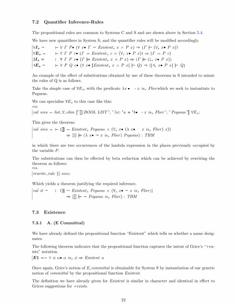
7.2 Quantifier Inference-Rules
The propositional rules are common to Systems C and S and are shown above in Section 5.4.
We have new quantifiers in System S, and the quantifier rules will be modified accordingly.
@Is � $ @ Γ P p@ x Γ |ù Existents x ^ P x q ñ pΓ |ù p@s x P x qq
@Es � $ @ Γ P c pΓ |ù Existents c ^ p@s x P x qq ñ pΓ |ù P cq
DIs � $ @ Γ P x pΓ |ù Existents x ^ P x q ñ pΓ |ù pDs x P x qq
DEs � $ @ P Q c p@ x rExistents x ^ P x s |ù Qq ñ prDs x P x s |ù Qq
An example of the effect of substitutions obtained by use of these theorems in S intended to mimicthe rules of Q is as follows.
Take ths simple case of @Es, with the predicate λx x iss Flierwhich we seek to instantiate toPegasus.
We can specialise @Es to this case like this:SML
val sves � list @ elim rprs:BOOL LISTq, pλx : 1a � 1b x iss Flierq, pPegasusqs @E s ;
This gives the theorem:
val sves � $ prs |ù Existents Pegasus ^ p@s x pλ x x iss Flierq x qq
ñ prs |ù pλ x x iss Flierq Pegasusq : THM
in which there are two occurrences of the lambda expression in the places previously occupied bythe variable P .
The substitutions can then be effected by beta reduction which can be achieved by rewriting thetheorem as follows:SML
rewrite rule rs sves;
Which yields a theorem justifying the required inference.
val it � $ prs |ù Existents Pegasus ^ p@s x x iss Flierqq
ñ prs |ù Pegasus iss Flierq : THM
7.3 Existence
7.3.1 A. (E Committal)
We have already defined the propositional function “Existent” which tells us whether a name desig-nates.
The following theorem indicates that the propositional function captures the intent of Grice’s “+ex-ists” notation.
E1 �$ @ φ α α iss φ ñ Existent α
Once again, Grice’s notion of E committal is obtainable for System S by instantiation of our genericnotion of committal by the propositional function Existent.
The definition we have already given for Existent is similar in character and identical in effect toGrices suggestions for +exists.
22

7.3.2 B. Existentially Quantified Formulae
This has already been covered.
Grice wishes to distinguish himself from Meinong, but his system allows quantification over non-existents, and he can therefore only distinguish himself from Meinong by distancing himself alsofrom Quine’s criteria of ontological committment. This he could easily do by adopting Carnap’sdistinction between internal and external questions, and denying that any metaphysical significanceattaches to something being counted in the range of quantification.
7.4 Identity
HOL already has identity and this identity is good for System C. It HOL it is a curried propositionalfunction of polymorphic type p :’aÑ ’aÑ BOOLq. If applied using function application the universallaw of reflexivity holds.
To get a “strict” version of equality (i.e. one which is false when either argument does not exist) itis necessary to uncurry equality so that its type becomes p :(’a � ’a) Ñ BOOLq and apply it usingthe system C copula for binary relations.
These two seem to correspond to Grice’s intended two kinds of equality insofar as the differencebetween the two is primarily that one does and the other does not allow that there may be trueidentities between non-denoting names. However this is achieved in system C by having two quitedistinct identity relations only one of which is properly a predicate, and applied through our copulaiss. The other is a propositional function which must be applied without use of the copula (becausethe copula forces strictness, i.e. forces predication to undefined values to yield falsehoods).
Grice seems to think that the required distinction between equalities can be achieved by the use ofhis scoping subscripts, but I have not yet been convinced that his is correct in this. Whatever thescope of the predicate, predication to non-denoting names must yield falsehood, so I can’t see howany use of subscripts will make “Pegasus = Pegasus” true.
To illustrate the effect of the built in equality the following theorems suffice:
Pegasus eq lemma1 �
$ Pegasus � Pegasus
Note the lack of copula. This is of course an instance of the theorem:
eq refl thm �
$ @ x x � x
To get a nice notation for “strong” equality we need to define it as an infix symbol, which requiresthat the copula be built into the definition. We could use the � symbol, but this usually represents anequivalence relation which is weaker than identity, so we will subscript the � sign with g, suggestingthat it is just the same thing applied through our copula.SML
declare infix p200 , "�s"q;
HOL Constant
$�s : SC Ñ SC Ñ BOOL
@x y :SC px �s yq � px ,yq iss2 pUncurry $�q
23

We can now prove:
Pegasus eq lemma2 �
$ Pegasus �s Pegasus
And must rest content with the qualified rule:
eqs refl thm �
$ @ x x iss Existent ô x �s x
The “strictness” of this equality is expressed by the theorem (which would have made a betterdefinition):
eqs strict thm �
$ @ x y x �s y ô x iss Existent ^ y iss Existent ^ x � y
The primitive equality in HOL no longer corresponds to Grice’s second order definition and the proofof snd order eq thm fails.
neg snd order eq thm �
$ p@ x y x � y ô p@ P x iss P ô y iss Pqq
There are two reasons for this. The first is that there is now more than one possible non-denotingcorrelate, and Leibniz’s formula, applied through the System S copula does not distinguish betweenthem. The second is the presence of values for failing descriptions.
The values for failing descriptions should not be in the range of quantification, so we do need tohave special quantifiers in System S, it will then also be necessary to qualify the quantification toget a version of the second order definition which takes account of possibly distinct non-designatingnames.
This equivalence fails because we now allow (in fact, require) more than one non-designating valuein the domain of an interpretation.
However, if the copula is dropped we still get a working definition of a ‘weak’ equality.
snd order eq thm2 �
$ @ x y x � y ô p@ P P x ô P yq
8 Conclusions
9 Postscript
These are the kinds of thing which might happen in future issues of this document:
• Much more detailed discussion and jusification of the method of formalisation, probably splitbetween here and an earlier chapter of the first volume.
• A full discussion of the philosophical issues.
• It would probably be better to rework with a different semantics, with type ’a+’b+’c, separatedisjuncts for designating, non-designating and non-correlating expressions, to allow for distinctnon-existents and descriptions.
24

A Theory Listings
A.1 The Theory grice
Parents
rbjmisc
Children
griceS griceC
Constants
$|ù BOOL LIST Ñ BOOL Ñ BOOL$committal p1a Ñ BOOLq Ñ p1a Ñ BOOLq Ñ BOOL
Fixity
Right Infix 4 : |ùRight Infix 100 :
committal
Definitions
|ù $ @ al c pal |ù cq ô @L al ñ ccommittal $ @ P φ P committal φ ô p@ α φ α ñ P αq
Theorems
ASS $ @ φ rφs |ù φRAA $ @ φ ψ ζ Γ prφs @ Γ |ù ψ ^ ψq ñ pΓ |ù φqDN $ @ φ r φs |ù φ^I $ @ φ ψ rφ; ψs |ù φ ^ ψ^E $ @ φ ψ prφ ^ ψs |ù φq ^ prφ ^ ψs |ù ψq_I $ @ φ ψ prφs |ù φ _ ψq ^ prφs |ù ψ _ φq_E $ @ φ ψ ζ Γ ∆ Θ
prφs @ Γ |ù ζq ^ prψs @ ∆ |ù ζq ^ pΘ |ù φ _ ψqñ pΓ @ ∆ @ Θ |ù ζq
CP $ @ φ ψ Γ prφs @ Γ |ù ψq ñ pΓ |ù φ ñ ψqMPP $ @ φ ψ rφ ñ ψ; φs |ù ψ@I $ @ Γ P p@ x Γ |ù P x q ñ pΓ |ù p@ x P x qq@E $ @ Γ P c pΓ |ù p@ x P x qq ñ pΓ |ù P cqDI $ @ Γ P x pΓ |ù P x q ñ pΓ |ù pD x P x qqDE $ @ P Q p@ x rP x s |ù Qq ñ prD x P x s |ù QqP 2 $ @ P φ P committal φ ñ P committal pλ α φ αqP 3 $ @ P φ ψ
P committal φ _ P committal ψñ P committal pλ α φ α ^ ψ αq
P 4 $ @ P φ ψ
25

P committal φ ^ P committal ψñ P committal pλ α φ α _ ψ αq
P 5 $ @ P φ ψ P committal pλ α φ αq ^ P committal ψ
ñ P committal pλ α φ α ñ ψ αqP 6@ $ @ P φ
pD β P committal φ βqñ P committal pλ α @ β φ β αq
P 6Db $ @ P φ p@ β P committal φ βq
ñ P committal pλ α D β φ β αq
26

A.2 The Theory griceC
Parents
grice
Constants
K 1a$isc
1a Ñ p1a Ñ BOOLq Ñ BOOL$isc2
1a � 1b Ñ p1a � 1b Ñ BOOLq Ñ BOOLPegasus 1aF lier 1a Ñ BOOLNonF lier 1a Ñ BOOLExistent 1a Ñ BOOL$�c
1a Ñ 1a Ñ BOOL$ι p1a Ñ BOOLq Ñ 1a
Fixity
Binder : ιRight Infix 200 :
�c
Right Infix 400 :isc isc2
Definitions
K $ Tisc $ @ p t t isc p ô pif t � K then F else p tqisc2 $ @ p t
t isc2 pô pif Fst t � K _ Snd t � K then F else p tq
Pegasus $ Pegasus � KF lier $ TNonF lier $ @ x NonFlier x ô Flier xExistent $ @ x Existent x ô T�c $ @ x y x �c y ô px , yq isc2 Uncurry $�ι $ @ φ
$ι φ� pε α α isc φ ^ p@ β β isc φ ñ β � αq
_ pD γ γ isc φ ^ p@ β β isc φ ñ β � γqq^ α � Kq
27

Theorems
Pegasus lemma 1$ Pegasus isc Flier ô F
Pegasus lemma 2$ Pegasus isc pλ x Flier x q ô F
Pegasus lemma 3$ Pegasus isc Flier
Pegasus lemma 4$ Pegasus isc pλ x Flier x q
Pegasus lemma 5$ Pegasus isc NonFlier ô F
Existent lemma 1$ @ P x x isc Existent ñ x isc P
D lemma 1 $ @ P Pegasus isc P ñ pD x x isc Pq@ lemma 1 $ @ P p@ x x isc Pq ñ Pegasus isc PE1 $ @ φ α α isc φ ñ α isc ExistentPegasus eq lemma1
$ Pegasus � Pegasuseq refl thm $ @ x x � xPegasus eq lemma2
$ Pegasus �c Pegasuseqc refl thm
$ @ x x isc Existent ô x �c xeqc strict thm
$ @ x y x �c y ô x isc Existent ^ y isc Existent ^ x � y
snd order eq thm$ @ x y x � y ô p@ P x isc P ô y isc Pq
snd order eq thm2$ @ x y x � y ô p@ P P x ô P yq
ι thm1 $ @ γ γ isc φ ^ p@ β β isc φ ñ β � γq ñ $ι φ � γι thm2 $ pD γ γ isc φ ^ p@ β β isc φ ñ β � γqq
ñ $ι φ � K
28

A.3 The Theory griceS
Parents
grice
Constants
denotatum 1a Ñ BOOLK corr 1aK SCIsCorr SC Ñ BOOLCorr SC Ñ 1aIsDen SC Ñ BOOL$iss SC Ñ p1a Ñ BOOLq Ñ BOOL$iss2 SC � SC Ñ p1a � 1a Ñ BOOLq Ñ BOOLPegasus SCF lier 1a Ñ BOOLNonF lier 1a Ñ BOOLExistent 1a Ñ BOOL$@s pSC Ñ BOOLq Ñ BOOL$Ds pSC Ñ BOOLq Ñ BOOLExistents SC Ñ BOOL$�s SC Ñ SC Ñ BOOL
Type Abbreviations
SC SC
Fixity
Binder : @s DsRight Infix 200 :
�s
Right Infix 400 :iss iss2
Definitions
denotatum $ D x denotatum xK corr $ denotatum K corrK $ K � InL K corrIsCorr $ @ v IsCorr v ô IsL vCorr $ @ v Corr v � OutL vIsDen $ @ v IsDen v ô IsCorr v ^ denotatum pCorr vqiss $ @ p t t iss p ô pif IsDen t then p pCorr tq else F qiss2 $ @ p t
t iss2 pô pif IsDen pFst tq ^ IsDen pSnd tq
then p pCorr pFst tq, Corr pSnd tqq
29

else F qPegasus $ IsCorr Pegasus ^ IsDen PegasusF lier $ TNonF lier $ @ x NonFlier x ô Flier xExistent $ @ x Existent x ô T@s $ @ f $@s f ô p@ x IsCorr x ñ f x qDs $ @ f $Ds f ô pD x IsCorr x ^ f x qExistents $ @ x Existents x ô pDs y x � yq�s $ @ x y x �s y ô px , yq iss2 Uncurry $�
Theorems
Pegasus lemma 1$ Pegasus iss Flier ô F
Pegasus lemma 2$ Pegasus iss pλ x Flier x q ô F
Pegasus lemma 3$ Pegasus iss Flier
Pegasus lemma 4$ Pegasus iss pλ x Flier x q
Pegasus lemma 5$ Pegasus iss NonFlier ô F
Existent lemma 1$ @ P x x iss Existent ñ x iss P
D lemma 1 $ @ P Pegasus iss P ñ pD x x iss Pq@ lemma 1 $ @ P p@ x x iss Pq ñ Pegasus iss PD not Corr thm
$ D x IsCorr x@Is $ @ Γ P
p@ x Γ |ù Existents x ^ P x q ñ pΓ |ù p@s x P x qq@Es $ @ Γ P c
pΓ |ù Existents c ^ p@s x P x qq ñ pΓ |ù P cqDIs $ @ Γ P x
pΓ |ù Existents x ^ P x q ñ pΓ |ù pDs x P x qqDEs $ @ P Q c
p@ x rExistents x ^ P x s |ù Qqñ prDs x P x s |ù Qq
E1 $ @ φ α α iss φ ñ Existent αPegasus eq lemma1
$ Pegasus � Pegasuseq refl thm $ @ x x � xPegasus eq lemma2
$ Pegasus �s Pegasuseqs refl thm
$ @ x x iss Existent ô x �s xeqs strict thm
$ @ x y x �s y ô x iss Existent ^ y iss Existent ^ x � y
neg snd order eq thm$ p@ x y x � y ô p@ P x iss P ô y iss Pqq
snd order eq thm2$ @ x y x � y ô p@ P P x ô P yq
30

A.4 *
Bibliography
[1] Alonzo Church. A Formulation of the Simple Theory of Types. Journal of Symbolic Logic,5:56–, 1940.
[2] Davidson and Hintikka, editors. Words and Objections: Essays on the work of W.V. Quine.Reidel Publishing. 1969.
[3] Richard E. Grandy and Richard Warner, editors. Philosophical Grounds of Rationality:Intentions, Categories, Ends. Clarendon Press. 1986.
[4] H.P. Grice. Vacuous Names. In Davidson and Hintikka [2].
[5] H.P. Grice. Studies in the Way of Words. Harvard University Press. 1989.
[6] Roger Bishop Jones. Analyses of Analysis: Part I - Introduction. RBJones.com, 2009-.http://www.rbjones.com/rbjpub/pp/doc/t029.pdf.
[7] Roger Bishop Jones. Analyses of Analysis: Part II - Synthetic Analysis. RBJones.com. 2009.http://www.rbjones.com/rbjpub/pp/doc/b003.pdf.
[8] Benson Mates. Elementary Logic. Oxford University Press. 1965.
[9] George Myro. Identity and Time. In Grandy and Warner [3].
[10] Bertrand Russell. On Denoting. [11].
[11] Bertrand Russell. Logic and Knowledge. Routledge. 1956.
31

A.5 *
Index� c . . . . . . . . . . . . . . . . . . . . . . . . . . . . . . . . . . . . . . 15, 27� s . . . . . . . . . . . . . . . . . . . . . . . . . . . . . . . . . . . 23, 29, 30K . . . . . . . . . . . . . . . . . . . . . . . . . . . . . . . . . 11, 18, 27, 29K corr . . . . . . . . . . . . . . . . . . . . . . . . . . . . . . . . . . 18, 29DE . . . . . . . . . . . . . . . . . . . . . . . . . . . . . . . . . . . . . . 10, 25DEs . . . . . . . . . . . . . . . . . . . . . . . . . . . . . . . . . . . . . 22, 30DI . . . . . . . . . . . . . . . . . . . . . . . . . . . . . . . . . . . . . . 10, 25DIs . . . . . . . . . . . . . . . . . . . . . . . . . . . . . . . . . . . . . . 22, 30D lemma 1 . . . . . . . . . . . . . . . . . . . . . . . . . 13, 20, 28, 30D not Corr thm . . . . . . . . . . . . . . . . . . . . . . . . . 21, 30Ds . . . . . . . . . . . . . . . . . . . . . . . . . . . . . . . . . . . . 21, 29, 30@E . . . . . . . . . . . . . . . . . . . . . . . . . . . . . . . . . . . . . . 10, 25@Es . . . . . . . . . . . . . . . . . . . . . . . . . . . . . . . . . . . . . 22, 30@I . . . . . . . . . . . . . . . . . . . . . . . . . . . . . . . . . . . . . . 10, 25@Is . . . . . . . . . . . . . . . . . . . . . . . . . . . . . . . . . . . . . 22, 30@ lemma 1 . . . . . . . . . . . . . . . . . . . . . . . . 13, 20, 28, 30@s . . . . . . . . . . . . . . . . . . . . . . . . . . . . . . . . . . . . 21, 29, 30ι . . . . . . . . . . . . . . . . . . . . . . . . . . . . . . . . . . . . . . . . 16, 27ι thm1 . . . . . . . . . . . . . . . . . . . . . . . . . . . . . . . . . . 17, 28ι thm2 . . . . . . . . . . . . . . . . . . . . . . . . . . . . . . . . . . 17, 28^E . . . . . . . . . . . . . . . . . . . . . . . . . . . . . . . . . . . . . 10, 25^I . . . . . . . . . . . . . . . . . . . . . . . . . . . . . . . . . . . . . . 10, 25_E . . . . . . . . . . . . . . . . . . . . . . . . . . . . . . . . . . . . . 10, 25_I . . . . . . . . . . . . . . . . . . . . . . . . . . . . . . . . . . . . . . 10, 25|ù . . . . . . . . . . . . . . . . . . . . . . . . . . . . . . . . . . . . . . . . . 25
ASS . . . . . . . . . . . . . . . . . . . . . . . . . . . . . . . . . . . . 10, 25
committal . . . . . . . . . . . . . . . . . . . . . . . . . . . . . . . 10, 25Corr . . . . . . . . . . . . . . . . . . . . . . . . . . . . . . . . . . . . 18, 29CP . . . . . . . . . . . . . . . . . . . . . . . . . . . . . . . . . . . . . 10, 25
denotatum . . . . . . . . . . . . . . . . . . . . . . . . . . . . . . . 17, 29difficulties . . . . . . . . . . . . . . . . . . . . . . . . . . . . . . . . . . 4DN . . . . . . . . . . . . . . . . . . . . . . . . . . . . . . . . . . . . . 10, 25
E1 . . . . . . . . . . . . . . . . . . . . . . . . . . . . . . . . 14, 22, 28, 30eq refl thm . . . . . . . . . . . . . . . . . . . . . . . 15, 23, 28, 30eqc refl thm . . . . . . . . . . . . . . . . . . . . . . . . . . . . . 16, 28eqc strict thm . . . . . . . . . . . . . . . . . . . . . . . . . . . . . . 28eqs refl thm . . . . . . . . . . . . . . . . . . . . . . . . . . . . . 24, 30eqs strict thm . . . . . . . . . . . . . . . . . . . . . . . . . . . . . . 30Existent . . . . . . . . . . . . . . . . . . . . . . . 13, 20, 27, 29, 30Existent lemma 1 . . . . . . . . . . . . . . . . . . 13, 20, 28, 30Existents . . . . . . . . . . . . . . . . . . . . . . . . . . . . . 21, 29, 30
Flier . . . . . . . . . . . . . . . . . . . . . . . . . . 12, 19, 27, 29, 30
inclinations . . . . . . . . . . . . . . . . . . . . . . . . . . . . . . . . . . 4IsCorr . . . . . . . . . . . . . . . . . . . . . . . . . . . . . . . . . . 18, 29IsDen . . . . . . . . . . . . . . . . . . . . . . . . . . . . . . . . . . . 18, 29isc . . . . . . . . . . . . . . . . . . . . . . . . . . . . . . . . . . . . . . . . . 27isc2 . . . . . . . . . . . . . . . . . . . . . . . . . . . . . . . . . . . . . . . . 27iss . . . . . . . . . . . . . . . . . . . . . . . . . . . . . . . . . . . . . . . . . 29iss2 . . . . . . . . . . . . . . . . . . . . . . . . . . . . . . . . . . . . . . . . 29
MPP . . . . . . . . . . . . . . . . . . . . . . . . . . . . . . . . . . . 10, 25
neg snd order eq thm . . . . . . . . . . . . . . . . . . . 24, 30NonFlier . . . . . . . . . . . . . . . . . . . . . . 13, 20, 27, 29, 30
objectives . . . . . . . . . . . . . . . . . . . . . . . . . . . . . . . . . . . . 5detailed . . . . . . . . . . . . . . . . . . . . . . . . . . . . . . . . . . . 5
P 2 . . . . . . . . . . . . . . . . . . . . . . . . . . . . . . . . . . . . . 11, 25P 3 . . . . . . . . . . . . . . . . . . . . . . . . . . . . . . . . . . . . . 11, 25P 4 . . . . . . . . . . . . . . . . . . . . . . . . . . . . . . . . . . . . . 11, 25P 5 . . . . . . . . . . . . . . . . . . . . . . . . . . . . . . . . . . . . . 11, 26P 6Db . . . . . . . . . . . . . . . . . . . . . . . . . . . . . . . . . . . 11, 26P 6@ . . . . . . . . . . . . . . . . . . . . . . . . . . . . . . . . . . . . 11, 26Pegasus . . . . . . . . . . . . . . . . . . . . . . . 12, 19, 27, 29, 30Pegasus eq lemma1 . . . . . . . . . . . . . . . . 15, 23, 28, 30Pegasus eq lemma2 . . . . . . . . . . . . . . . . . . . . . . 28, 30Pegasus lemma 1 . . . . . . . . . . . . . . . . . . 13, 20, 28, 30Pegasus lemma 2 . . . . . . . . . . . . . . . . . . 13, 20, 28, 30Pegasus lemma 3 . . . . . . . . . . . . . . . . . . 13, 20, 28, 30Pegasus lemma 4 . . . . . . . . . . . . . . . . . . 13, 20, 28, 30Pegasus lemma 5 . . . . . . . . . . . . . . . . . . 13, 20, 28, 30
RAA . . . . . . . . . . . . . . . . . . . . . . . . . . . . . . . . . . . . 10, 25resolutions . . . . . . . . . . . . . . . . . . . . . . . . . . . . . . . . . . 5
SC . . . . . . . . . . . . . . . . . . . . . . . . . . . . . . . . . . . . . . . . . 29snd order eq thm . . . . . . . . . . . . . . . . . . . . . . . 16, 28snd order eq thm2 . . . . . . . . . . . . . . . . 16, 24, 28, 30STT . . . . . . . . . . . . . . . . . . . . . . . . . . . . . . . . . . . . . . . . 6
32