Grey Numbers in Multiple CriteriaDecision Analysis and Conflict

Resolution

by

Hanbin Kuang

A thesispresented to the University of Waterloo

in fulfillment of thethesis requirement for the degree of

Doctor of Philosophyin

Systems Design Engineering

Waterloo, Ontario, Canada, 2014

c© Hanbin Kuang 2014

Author’s Declaration

I hereby declare that I am the sole author of this thesis. This is a true copy of the thesis,including any required final revisions, as accepted by my examiners.

I understand that my thesis may be made electronically available to the public.

ii

Abstract

Definitions of grey numbers are adapted for incorporation into Multiple Criteria Deci-

sion Analysis (MCDA) and the Graph Model for Conflict Resolution (GMCR) in order to

capture uncertainty in decision making. The main objective is to design improved meth-

ods for dealing with decision problems under uncertainty, characterized by limited input

data and uncertain preferences of decision makers (DMs). A literature review is carried

out in order to understand the problems of representing uncertainty using grey numbers

within two key decision making contexts: comparing alternative solutions within an MCDA

framework, and deciding upon meaningful courses of action by DMs involved in a conflict.

Then two methodologies that rely on grey numbers to represent uncertain information are

provided, and relevant definitions, procedures, and solution concepts are presented.

A new approach to handling uncertainty in MCDA using grey numbers is proposed.

The grey-based PROMETHEE II methodology is designed to represent and analyze multi-

criteria decision problems under uncertainty. The basic structure of a grey decision system

is developed, including definitions, notation, and detailed calculation procedures. By inte-

grating continuous grey numbers with linguistic expressions, each DM’s uncertain prefer-

ence can be expressed according to multiple criteria. The new methodology takes account

of both quantitative and qualitative data, first aggregating the DMs’ judgements on the

performance of alternatives according to each criterion, and then integrating the criteria

in order to determine the relative preference of any two alternatives. These preferences are

then incorporated into the PROMETHEE II methodology to generate a complete rank-

ing of alternatives. The procedure is illustrated using a case study in which source water

protection strategies are ranked for the Region of Waterloo, Ontario, Canada.

To capture uncertainty in preferences, definitions based on grey numbers are incor-

porated into GMCR, a realistic and flexible methodology to model and analyze strategic

conflicts. A general grey number, consisting of either discrete real numbers or intervals

of real numbers, or combinations of them, can represent the preferences of DMs in a very

general way. In analyzing a strategic conflict, the relative preference of each DM with re-

spect to feasible states is required before a stability analysis can be carried out. However,

because of incomplete information regarding many conflict situations, cognitive limitations

iii

of DMs, the interplay of stakeholders and the complexity of disputes in reality, it is hard

to capture accurate preferences of all DMs across all possible scenarios, or states. Here, a

grey-based preference structure is developed and integrated into GMCR. Utilizing a num-

ber of grey-based concepts, stability definition describing human behaviour under conflict

in the face of uncertain preference are introduced for a 2-DM conflict model. This Grey-

based GMCR is then applied to a generic sustainable development conflict with uncertain

preferences in order to demonstrate how it can be conveniently utilized in practice.

Then the definition of grey preference is incorporated into GMCR in a multiple-DM

context in order to model and represent uncertain human behaviour in a more complex

strategic conflict. When more than two DMs are involved, coordinated moves against a

focal DM need to be taken into account when calculating stable states. In this research,

a preference structure based on grey numbers is extended to represent multiple DMs’ un-

certain preferences for which there can be two or more DMs. Then four kinds of grey

stabilities (grey Nash stability, grey general metarationality, grey symmetric metarational-

ity, and grey sequential stability) and corresponding equilibria are defined for a grey-based

conflict model with multiple DMs. The feasibility of this methodology is verified through

a case study of a brownfield redevelopment conflict in Kitchener, Ontario, Canada.

iv

Acknowledgements

I would like to express my sincere gratitude to my supervisors, Professor Keith W.

Hipel and Professor D. Marc Kilgour, for their inspiration, encouragement, guidance and

friendship throughout my PhD program and the completion of this research. It is my great

honour and distinct pleasure to express my appreciation for their support.

I wish to thank my external examiner, Dr. Adiel Teixeira de Almeida of the Uni-

versidade Federal de Pernambuco in Brazil, and the other committee members from the

University of Waterloo, consisting of Dr. Mahesh Pandey of the Department of Civil and

Environmental Engineering, as well as Dr. Jonathan Histon and Dr. John Zelek of the

Department of Systems Design Engineering, for carefully reading my thesis and providing

helpful suggestions for improving it.

I wish to extend my gratitude to the secretarial and technical staff of the Department

of Systems Design Engineering for their professional service and support. I am especially

thankful for the assistance of Ms. Vicky Lawrence, Ms. Colleen Richardson, and Ms. Angie

Muir. I also want to acknowledge the China Scholarship Council (NSCIS No 2010683003)

for the financial support during my PhD. study, and the education office of the Consulate

General of the People’s Republic of China in Toronto for their consulting services. I really

appreciate the help from Ms. Min Chen.

I am most grateful to my friend and colleague, Dr. M. Abul Bashar, for his valuable

suggestions on refining various technical parts in my thesis. My appreciation also goes to

my friends for their companionship and support throughout the course of my studies in

Canada.

In addition, I express my sincere appreciation to Mrs. Joan Kilgour, whose tutorials

helped me to improve my English pronunciation, writing, and grammar. Her kind and

v

insightful suggestions upgraded the quality of my work. I would also like to thank Mr.

Conrad Hipel for editing some my research papers.

I cannot end without thanking my parents, Mr. Baohe Kuang and Ms. Suqin Han, my

grandparents, Mr. Yulin Han and Ms. Guilan Zheng, and my fiancee, Ms. Chenxu Dang,

for their constant encouragement and love.

vi

Table of Contents

List of Tables xi

List of Figures xiv

1 Introduction 1

1.1 Problem Statement . . . . . . . . . . . . . . . . . . . . . . . . . . . . . . . 4

1.2 Research Objectives . . . . . . . . . . . . . . . . . . . . . . . . . . . . . . . 6

1.3 Thesis Organization . . . . . . . . . . . . . . . . . . . . . . . . . . . . . . . 8

2 Grey Systems Theory and Multiple Criteria Decision Analysis 11

2.1 Grey Systems Theory . . . . . . . . . . . . . . . . . . . . . . . . . . . . . . 11

2.1.1 Fundamental Concepts . . . . . . . . . . . . . . . . . . . . . . . . 12

2.1.2 Grey Relational Analysis . . . . . . . . . . . . . . . . . . . . . . . . 20

2.2 Multiple Criteria Decision Analysis . . . . . . . . . . . . . . . . . . . . . . 25

2.2.1 Review of MCDA Approaches . . . . . . . . . . . . . . . . . . . . . 26

2.2.2 PROMETHEE Modelling . . . . . . . . . . . . . . . . . . . . . . . 28

vii

2.3 Conclusions . . . . . . . . . . . . . . . . . . . . . . . . . . . . . . . . . . . 30

3 The Grey-based PROMETHEE II Methodology 32

3.1 Introduction . . . . . . . . . . . . . . . . . . . . . . . . . . . . . . . . . . . 32

3.2 Grey-based PROMETHEE II Methodology . . . . . . . . . . . . . . . . . . 34

3.2.1 Structure of the Grey Decision System . . . . . . . . . . . . . . . . 34

3.2.2 Normalizing the Performance of Alternatives . . . . . . . . . . . . . 36

3.2.3 Ranking Alternatives based on PROMETHEE II

Methodology . . . . . . . . . . . . . . . . . . . . . . . . . . . . . . 42

3.3 Case illustration of Evaluation of Source Water Protection Strategies . . . 46

3.3.1 Background . . . . . . . . . . . . . . . . . . . . . . . . . . . . . . . 46

3.3.2 Input Data . . . . . . . . . . . . . . . . . . . . . . . . . . . . . . . 48

3.3.3 Normalization of the Performance of Alternatives . . . . . . . . . . 50

3.3.4 Results and Analysis . . . . . . . . . . . . . . . . . . . . . . . . . . 51

3.4 Conclusions . . . . . . . . . . . . . . . . . . . . . . . . . . . . . . . . . . . 54

4 The Graph Model for Conflict Resolution 56

4.1 Introduction . . . . . . . . . . . . . . . . . . . . . . . . . . . . . . . . . . . 56

4.2 Theoretical Foundations of the Graph Model for Conflict Resolution . . . . 57

4.3 Stability Analysis in a Conflict with Two Decision Makers . . . . . . . . . 60

4.4 Stability Analysis in a Conflict with Multiple

Decision Makers . . . . . . . . . . . . . . . . . . . . . . . . . . . . . . . . . 62

viii

4.5 Case Study: Conflict Analysis on Water Use and Oil Sands Development in

the Athabasca River . . . . . . . . . . . . . . . . . . . . . . . . . . . . . . 64

4.5.1 Background . . . . . . . . . . . . . . . . . . . . . . . . . . . . . . . 64

4.5.2 Water Use and Oil Sands Development Conflict in the Athabasca

River Basin . . . . . . . . . . . . . . . . . . . . . . . . . . . . . . . 66

4.5.3 Stability Analysis . . . . . . . . . . . . . . . . . . . . . . . . . . . . 74

4.6 Conclusions . . . . . . . . . . . . . . . . . . . . . . . . . . . . . . . . . . . 76

5 Grey-based Preference in a Graph Model for Conflict Resolution with

Two Decision Makers 77

5.1 Grey Preference Structure in the Graph Model . . . . . . . . . . . . . . . . 79

5.1.1 Grey Preference Degree . . . . . . . . . . . . . . . . . . . . . . . . . 80

5.1.2 Grey Relative Certainty of Preference . . . . . . . . . . . . . . . . . 83

5.1.3 Grey Unilateral Improvement . . . . . . . . . . . . . . . . . . . . . 85

5.2 Grey Stabilities in a Conflict with Two Decision Makers . . . . . . . . . . 88

5.3 Case Study: Sustainable Development Conflict under Uncertainty . . . . . 93

5.3.1 Background . . . . . . . . . . . . . . . . . . . . . . . . . . . . . . . 93

5.3.2 Graph Model with Uncertainty . . . . . . . . . . . . . . . . . . . . 95

5.3.3 Stability Analysis . . . . . . . . . . . . . . . . . . . . . . . . . . . . 97

5.3.4 Insights and Sensitivity Analysis . . . . . . . . . . . . . . . . . . . . 98

5.4 Conclusions . . . . . . . . . . . . . . . . . . . . . . . . . . . . . . . . . . . 100

ix

6 Grey-based Preference in a Graph Model for Conflict Resolution with

Multiple Decision Makers 102

6.1 Grey-based Graph Model for Conflict Resolution with Multiple Decision

Makers . . . . . . . . . . . . . . . . . . . . . . . . . . . . . . . . . . . . . . 102

6.1.1 Grey Unilateral Improvements for a Conflict with Multiple Decision

Makers . . . . . . . . . . . . . . . . . . . . . . . . . . . . . . . . . . 103

6.1.2 Grey Stabilities Definitions and Equilibria . . . . . . . . . . . . . . 106

6.2 Negotiation of Brownfield Redevelopment

Conflict under Uncertainty . . . . . . . . . . . . . . . . . . . . . . . . . . . 109

6.2.1 Background of Kaufman Site Redevelopment Conflict . . . . . . . . 109

6.2.2 Grey-based Uncertain Preferences for the Decision Makers . . . . . 112

6.2.3 Stability Analysis of the Brownfield Redevelopment

Conflict . . . . . . . . . . . . . . . . . . . . . . . . . . . . . . . . . 118

6.2.4 Status Quo Analysis . . . . . . . . . . . . . . . . . . . . . . . . . . 126

6.3 Conclusions . . . . . . . . . . . . . . . . . . . . . . . . . . . . . . . . . . . 128

7 Contributions and Future Research 129

7.1 Main Contributions . . . . . . . . . . . . . . . . . . . . . . . . . . . . . . . 129

7.2 Future Research Plan . . . . . . . . . . . . . . . . . . . . . . . . . . . . . . 132

References 134

x

List of Tables

2.1 Grey Relational Analysis Structure . . . . . . . . . . . . . . . . . . . . . . 21

3.1 Grey-based Decision Structure . . . . . . . . . . . . . . . . . . . . . . . . . 35

3.2 Grey-based Performance Matrix by DM l on Qualitative Criteria . . . . . . 39

3.3 The Importance Degree of DM l . . . . . . . . . . . . . . . . . . . . . . . . 40

3.4 Performance of Alternative i on Qualitative Criterion j Evaluated by Deci-

sion Maker l . . . . . . . . . . . . . . . . . . . . . . . . . . . . . . . . . . . 40

3.5 Importance Degrees of Decision Makers . . . . . . . . . . . . . . . . . . . . 48

3.6 Weights of Criteria . . . . . . . . . . . . . . . . . . . . . . . . . . . . . . . 49

3.7 Performance of Source Water Protection Strategies on Qualitative Criteria 49

3.8 Performance of Source Water Protection Strategies on Quantitative Criteria 50

3.9 Normalized Importance Degrees of Decision Makers . . . . . . . . . . . . . 50

3.10 Normalized Performance of Alternatives on Criteria . . . . . . . . . . . . . 51

3.11 Multiple Criteria Preference Matrix . . . . . . . . . . . . . . . . . . . . . . 52

3.12 Netflow of Alternatives . . . . . . . . . . . . . . . . . . . . . . . . . . . . . 53

xi

4.1 Decision Makers and Their Options . . . . . . . . . . . . . . . . . . . . . . 69

4.2 Decision Makers, Options and Feasible States . . . . . . . . . . . . . . . . 70

4.3 Preference Ordering Principals for the Alberta Government . . . . . . . . . 71

4.4 Preference Ordering Principals for Oil Sands Companies . . . . . . . . . . 72

4.5 Preference Ordering Principals for NGOs . . . . . . . . . . . . . . . . . . . 72

4.6 Stability Results for the conflict of water use and oil sands development . . 75

5.1 Feasible States for the Sustainable Development Conflict . . . . . . . . . . 94

5.2 Grey Preference Matrices of ENV and DEV . . . . . . . . . . . . . . . . . 96

5.3 Grey relative certainty of Preferences of ENV and DEV . . . . . . . . . . . 97

5.4 Stability Results for the Sustainable Development Conflict under Uncer-

tainty - with Neutral DEV . . . . . . . . . . . . . . . . . . . . . . . . . . . 98

5.5 Stability Findings for the Sustainable Development Conflict under Uncer-

tainty - with Pessimistic DEV . . . . . . . . . . . . . . . . . . . . . . . . . 100

5.6 Stability Results for the Sustainable Development Conflict under Uncer-

tainty - with Optimistic DEV . . . . . . . . . . . . . . . . . . . . . . . . . 101

6.1 DMs, Options, and States in the Acquisition Conflict of Brownfield Rede-

velopment (Modified from (Bernath Walker et al., 2010)) . . . . . . . . . . 111

6.2 Grey Preference Matrices of PO . . . . . . . . . . . . . . . . . . . . . . . . 113

6.3 Grey Preference Matrices of CG . . . . . . . . . . . . . . . . . . . . . . . . 114

6.4 Grey Preference Matrices of D . . . . . . . . . . . . . . . . . . . . . . . . . 115

xii

6.5 Grey Relative Preference Matrices of PO . . . . . . . . . . . . . . . . . . . 116

6.6 Grey Relative Preference Matrices of CG . . . . . . . . . . . . . . . . . . . 117

6.7 Grey Relative Preference Matrices of D . . . . . . . . . . . . . . . . . . . . 117

6.8 Anticipated Preferences of the Decision Makers in the Conflict . . . . . . . 119

6.9 Stability Results for Brownfield Redevelopment Conflict under Uncertainty 123

6.10 Status Quo Analysis . . . . . . . . . . . . . . . . . . . . . . . . . . . . . . 127

xiii

List of Figures

1.1 Thesis Organization . . . . . . . . . . . . . . . . . . . . . . . . . . . . . . . 10

2.1 Distinguishing Grey Numbers from Probability Distributions and Fuzzy

Numbers . . . . . . . . . . . . . . . . . . . . . . . . . . . . . . . . . . . . . 16

2.2 Grey Relational Degree: Reference Sequence versus Alternatives (Zhai et al.,

2009) . . . . . . . . . . . . . . . . . . . . . . . . . . . . . . . . . . . . . . . 20

3.1 Flow Chart of Grey-based PROMETHEE II Methodology . . . . . . . . . 33

3.2 The Preference Degree of Alternative a over Alternative b . . . . . . . . . . 44

4.1 Integrated Transitional Graph of Water Use and Oil Sands Development

Conflict in the Athabasca River Basin . . . . . . . . . . . . . . . . . . . . . 73

5.1 Main Contributions within the Framework of Conflict Analysis . . . . . . . 78

5.2 The Graph Model of Movement for the Sustainable Development Conflict . 95

6.1 A Graph Model for a Simple Conflict . . . . . . . . . . . . . . . . . . . . . 104

6.2 Flow Chart for grey-based Graph Model for Conflict Resolution . . . . . . 108

xiv

6.3 Integrated Directed Graph of the Property Acquisition Conflict (Modified

from (Bernath Walker et al., 2010)) . . . . . . . . . . . . . . . . . . . . . . 112

6.4 Directed Graph for PO Holding Different Grey Satisficing Thretholds . . . 120

6.5 Directed Graph for D Holding Different Grey Satisficing Thretholds . . . . 121

6.6 Directed Graph for CG Holding Different Grey Satisficing Thretholds . . . 122

6.7 Grey Unilateral Improvements and Potential Sanctions (GST: PO = 0.1, D

= 0.6, CG = 0.2) . . . . . . . . . . . . . . . . . . . . . . . . . . . . . . . . 124

6.8 Grey Unilateral Improvements and Protential Sanctions for DMs (GST: PO

= 0.1, D = 0.6, CG = 0.2) . . . . . . . . . . . . . . . . . . . . . . . . . . . 125

6.9 Grey Unilateral Improvements and Protential Sanctions for DMs (GST: PO

= 0.9, D = 0.8, CG = 0.6) . . . . . . . . . . . . . . . . . . . . . . . . . . . 126

xv

Chapter 1

Introduction

Decision making is a central activity in the daily lives of most human beings, especially in

fields like economics and management. It can be considered to be a systematic process of

identifying and selecting alternatives according to available information or preferences of a

decision maker (DM) or multiple DMs (Janis and Mann, 1977). Decision theories are gen-

erally classified into three categories: normative, descriptive and prescriptive. A normative

decision theory indicates how a decision should be made in theory, on the assumption that

a DM is fully rational; a descriptive decision theory describes what a DM actually does

in specific situations; and a prescriptive decision theory concentrates on how a DM ought

to act with the purpose of improving the outcomes, despite imperfect information (Baron,

2000; Pratt et al., 1995; Tversky and Kahneman, 1986). With the development of decision

theories, it is hard to strictly characterize them according to the three aforementioned cat-

egories. This research focuses on refining normative and prescriptive theories and making

them more suitable to reflect modern decision problems.

In real-world applications, decision problems are frequently vast, complex and ill-

1

defined. Taking source water protection as an example, both tangible and intangible

criteria must be considered by DMs, including benefits; investment costs; projected op-

erating costs; water quantity and quality risks; and technical, operational, legal and so-

cial feasibility. Hipel et al. (1993) suggested four factors that affect the circumstances in

which a decision problem must be addressed: (i) whether the context includes uncertainty;

(ii) whether the courses of action can be completely assessed in quantitative terms; (iii)

whether multiple objectives must be taken into account; and (iv) whether a single DM or

multiple DMs are involved. Based on these factors, decision methodologies are classified

into four categories: single participant—single criterion, single participant—multiple cri-

teria, multiple participants—single criterion, and multiple participants—multiple criteria.

In principle, Multiple Criteria Decision Analysis (MCDA) is a single participant—

multiple criteria decision making technique, although it can easily be adopted for use by a

group of DMs (Belton and Pictet, 1997). MCDA constitutes a methodology that includes

techniques to guide DMs in identifying and structuring decision problems, and in explicitly

aggregating and evaluating multiple alternatives in decision environments (Guitouni and

Martel, 1998; Steward, 1992; Ozernoy, 1992). During the last 40 years, scientists and

practitioners not only accelerated the theoretical and technical development of MCDA

within the field of Operational Research and elsewhere, but also gained valuable experience

through applications to decision problems in many areas including environmental sciences,

social sciences, education, and health care (Flores-Alsina et al., 2008).

When two or more DMs are involved in a decision situation, a conflict may arise as the

DMs interact with others to further their own interests, which are often different (Hipel,

2009a; Kilgour and Eden, 2010). Each DM may have his or her own criteria to determine

preference among the possible scenarios. Hence, each DM may have his or her multiple

criteria decision problem to rank scenarios. Strategic conflicts are interactive decision

2

problems, in which each DM controls one or more options and attempts to achieve the

most preferable scenario. Note that if one DM exercises an option, it may benefit or harm

other DMs. Therefore, cooperative or compromise solutions may be available (Kilgour and

Hipel, 2005). In practice, these phenomena arise frequently, such as in military strategy,

business negotiation, and environmental management (Hipel et al., 1997; Kilgour et al.,

1987; Kassab et al., 2006).

The Graph Model for Conflict Resolution (GMCR) constitutes a simple and flexible

methodology to model and analyze strategic conflicts (Kilgour et al., 1987). Much valuable

research has been conducted on different aspects of this methodology both in theory and

in practice (Kilgour et al., 1987). Fang et al. (1993) focused on solution concepts and

their interrelationships as well as on how to apply GMCR in practice. Hipel et al. (2009)

explained the roles of GMCR and other Operational Research tools to solve problems within

a systems engineering context. Kilgour and Hipel (2005) reviewed various initiatives within

the GMCR framework and suggested guidelines for future development. To implement the

graph model methodology, a user-friendly decision support software, GMCR II, has been

developed. It can quickly, completely and reliably model and analyze multiple participant-

multiple criteria problems, large or small (Fang et al., 2003a,b).

As a researcher focusing on a class of decision making methodologies aiming to give

advice and suggestions to DMs, the author believes that if DMs provide enough informa-

tion, an optimal result should be obtained; even if DMs’ understanding of the problem is

limited by incomplete information and uncertainties, reasonable and satisfactory solutions

may be available; but if DMs have no information at all, they may have to rely on courage.

Reasonable decision methodologies focusing on uncertainty must be considered along with

our limited understanding of human cognition and the complexity of real applications in

which multiple DMs interact. Uncertainty and conflicts of interest among stakeholders

3

may complicate the analysis. Consequently, a satisfactory decision negotiated through

compromises and trade-offs, which better corresponds to the real world, may be a valuable

contribution to the DMs, even if it is not individually optimal.

1.1 Problem Statement

Originally, decision analysis techniques and methodologies were designed for tackling highly

structured problems using mathematical procedures to make rational choices based on

quantitative data (Checkland, 1981; Hipel et al., 1993; Radford, 1988). The modern solu-

tion objective for a decision problem is no longer optimality within a well-defined structure,

but satisfaction of DMs under complex circumstances in which qualitative criteria and in-

teraction with other DMs must be considered (Hipel et al., 1993). This research aims

to design new or improved methods for MCDA problems with uncertain information, or

for conflict resolution having uncertain preferences. In decision analysis, one of the main

difficulties is to incorporate uncertainty into decision processes. The natural complexity

of multiple criteria assessment and conflict resolution calls for the development of effective

and reliable techniques for handling decision problems under uncertainty (Ben-Haim and

Hipel, 2002; Hyde, 2006). To address these problems, this thesis begins by classifying un-

certainties in decision problems into three types according to the literature (Calizay et al.,

2010; Comes et al., 2011; Ekel et al., 2008), as follows:

• Deficient Understanding of the Decision Structure: Designing and selecting

a mathematical structure is the first step in modelling a decision problem. A logical,

well-defined structure based on well-conducted background research and practical

experience can catch the essence of a problem, accelerate the decision process, and

4

accordingly win the trust of stakeholders. On the contrary, an unsatisfactory struc-

ture may produce an unjustified recommendation, and mislead or disappoint DMs.

However, even a good structure may eventually be improved with deeper understand-

ing and further technical development (Ozernoy, 1992).

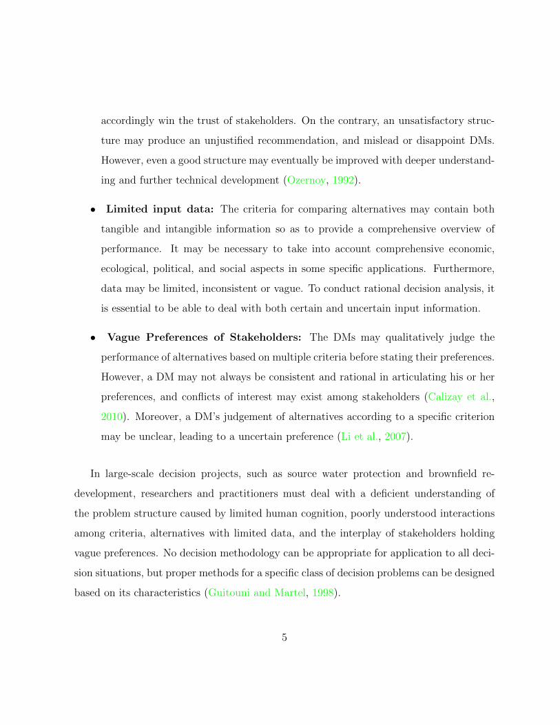
• Limited input data: The criteria for comparing alternatives may contain both

tangible and intangible information so as to provide a comprehensive overview of

performance. It may be necessary to take into account comprehensive economic,

ecological, political, and social aspects in some specific applications. Furthermore,

data may be limited, inconsistent or vague. To conduct rational decision analysis, it

is essential to be able to deal with both certain and uncertain input information.

• Vague Preferences of Stakeholders: The DMs may qualitatively judge the

performance of alternatives based on multiple criteria before stating their preferences.

However, a DM may not always be consistent and rational in articulating his or her

preferences, and conflicts of interest may exist among stakeholders (Calizay et al.,

2010). Moreover, a DM’s judgement of alternatives according to a specific criterion

may be unclear, leading to a uncertain preference (Li et al., 2007).

In large-scale decision projects, such as source water protection and brownfield re-

development, researchers and practitioners must deal with a deficient understanding of

the problem structure caused by limited human cognition, poorly understood interactions

among criteria, alternatives with limited data, and the interplay of stakeholders holding

vague preferences. No decision methodology can be appropriate for application to all deci-

sion situations, but proper methods for a specific class of decision problems can be designed

based on its characteristics (Guitouni and Martel, 1998).

5

1.2 Research Objectives

This research attempts to employ and customize grey systems theory to produce method-

ologies for solving decision problems under uncertainty and to use grey numbers in grey

systems theory to construct a more general uncertain structure with application to chal-

lenging decision issues arising in engineering and other fields. Up to now, there has been

no systematic application of grey systems theory techniques to MCDA and GMCR, and

researchers have paid little attention to important theoretical concepts related to grey

systems theory, such as grey sets and grey numbers.

Grey systems theory constitutes a valuable alternative for representing uncertainty in

modelling decision problems. Grey systems theory can provide an insightful view of decision

problems and accordingly help DMs understand their decision structure, rearrange their

strategies, reinforce their models, and make reasonable choices. The basic concepts of grey

systems theory can effectively deal with representation and processing of both vague and

incomplete information. The distinctions of grey systems theory with other methodologies

are further explained as follows:

• In semi-structured or unstructured decision problems, information may be uncertain

(Klein, 2008). Grey systems theory can effectively represent quantitative and qualita-

tive information and express uncertainty in a general way. Therefore, this method is

more suitable for the evaluation and assessment of alternatives (Liu and Lin, 2010).

• Most of the time, a DM may offer imprecise information, which can be represented

by sets of values, intervals of values or combinations of them. The linguistic method

is a widely accepted technique to represent DMs’ uncertain preference over alterna-

tives (Wei, 2011). This method requires relatively low cognitive effort and perfectly

6

matches the characteristics of grey systems theory. Grey systems theory can assess

linguistic values of alternatives based on the theorems, and operating rules of grey

numbers, thereby exploiting calculation processes to rank alternatives through the

effective combination of grey systems theory and other MCDA techniques.

• A grey number can represent both discrete values and interval values. Some real-

world problems may require the selection of one value among a limited number of

options. For example, there are three coloured balls in a black bag, and you must

pick one of them. Suppose each ball is either red or black. If you pick one of them,

the number of red balls you have is a discrete grey number, which must equal 0 or 1.

This kind of problem can be easily represented by discrete grey numbers. Moreover,

a generalised grey number may represent a preference in a conflict with discrete

values, interval values, or any of their combinations. Based on general grey numbers,

a general preference structure can be set up in GMCR.

Based on the characteristics of grey systems theory, theoretical research will be carried

out in this thesis starting with the definition of a grey number, and incorporating it into

MCDA and GMCR. The methods of grey systems theory, such as grey relational analysis

and the grey target decision method, will be investigated systemically and combined with

typical MCDA techniques to identify preferred or indifferent alternatives, to eliminate infe-

rior alternatives, and to determine alternatives reflecting potential compromises in MCDA

under uncertainty. Moreover, grey-based preference methods and related methodologies

will be developed in the context of GMCR. A new uncertain preference structure will be

constructed based on generalized grey numbers, thereby permitting moves and counter

moves of DMs with uncertain preferences to be discussed, and solution concepts to be put

forward. This research will also take a practical perspective, by combining grey systems

7

theory with other techniques and applying them to specific problems.

1.3 Thesis Organization

The thesis consists of seven chapters. Its organisation is shown in Figure 1.1.

• This thesis begins (Chapter 1) with a general introduction to decision problems to

provide a motivation for the research and setting out the objectives.

• Chapter 2 reviews some mainstream methods and describes fundamental notation

and definitions of MCDA and grey systems theory.

• Chapter 3 proposes a grey-based Preference Ranking Organization Method for En-

richment Evaluations (PROMETHEE) II methodology to handle multiple criteria

decision problems with ill-defined information. A case study regarding the evalua-

tion of source water protection strategies is presented to show the feasibility of this

methodology.

• Chapter 4 reviews the fundamental concepts and stability definitions of a graph

model. A conflict on water use and oil sands development in the Athabasca River in

Alberta, Canada, is developed and analyzed to show how this methodology can be

applied to strategic conflicts.

• Chapter 5 puts forward a grey-based GMCR model. In this methodology, a grey-

based preference structure is provided based on generalized grey numbers, and sta-

bility definitions are introduced in a graph model for conflict resolution having two

DMs.

8

• Chapter 6 extends the grey-based preference structure to represent uncertain prefer-

ences when multiple DMs are involved in a conflict. Appropriate solution concepts

are defined in grey-based GMCR with two or more DMs.

• Chapter 7 summaries the key research contributions contained in this thesis and puts

forward suggestions for future work.

9

Figure 1.1: Thesis Organization

10

Chapter 2

Grey Systems Theory and Multiple

Criteria Decision Analysis

In this chapter, two families of methodologies are summarised: Grey Systems Theory

and Multiple Criteria Decision Analysis (MCDA). In each section, essential literature is

reviewed and classified, and mathematical notation and definitions are provided along with

detailed explanation.

2.1 Grey Systems Theory

Grey Systems Theory, originally put forward by Deng (1982), is a methodology that fo-

cuses on addressing problems with imperfect numerical information, which may be discrete

or continuous (Deng, 1989; Liu and Forrest, 2010). In grey systems theory, a system with

information that is certain is called a White System; a system with information that is to-

tally unknown is referred to as a Black System; a system with partially known and partially

11

unknown information is called a Grey System. The theory contains five main parts: Grey

Prediction Models, Grey Relational Analysis (GRA), Grey Models for Decision Making,

Grey Game Models, and Grey Control Systems (Liu and Forrest, 2010). The methodolo-

gies can effectively handle representation and processing of vague or uncertain information,

and it can give insights into operational features of systems and their evolution.

A crucial feature of a method for solving decision problems under uncertainty is how it

deals with uncertain information (Greco et al., 2001). Grey systems theory, in particular,

possesses many desirable characteristics. Firstly, it can handle uncertain problems with

small samples and poor information. Secondly, grey numbers can represent not only one

or more discrete values but also intervals of numbers, depending on the DMs’ opinions.

Thirdly, grey systems theory uses the concept of degree of greyness to estimate the uncer-

tainty of grey numbers, rather than a typical distribution of their values (Liu and Forrest,

2010; Yang and John, 2012). However, most researchers and practitioners focus on grey

relational analysis and its combination with other techniques, with little attention paid to

theoretical foundations and extensions of definitions of grey numbers and associated theo-

rems to make them more suitable to decision analysis or conflict resolution. The following

subsection will systematically review mathematical concepts of grey systems theory with

examples to make them easier to understand.

2.1.1 Fundamental Concepts

This research presents fundamental grey concepts, including the definitions and theorems

of grey numbers, core of grey numbers, degree of greyness, and grey sets. A definition of

general grey number put forward by Yang et al. (2004) is also introduced in this section.

After that, the method of grey relational analysis is reviewed. This method is particularly

12

applicable in decision problems with very limited data and vague information.

Grey Numbers

A grey number is the most fundamental concept in grey systems theory. In the original

definitions, a white number is a real number, x ∈ R. A grey number, written ⊗x, means an

indeterminate real number that takes its possible values within an interval or a discrete set

of numbers. Let G[R] denotes the set of all grey numbers within the set of real numbers,

R, the definitions of discrete grey numbers, continuous grey numbers, and general grey

numbers are presented as follows:

Definition 2.1 A discrete grey number ⊗x is an unknown real number with a clear lower

bound x− and an upper bound x, x−, x ∈ R, taking its value from the closed interval, [x−, x],

denoted (Liu and Forrest, 2010):

⊗ x ∈ x1, x2, ..., xk (2.1)

Note that the lower bound x− = minixi and the upper bound x = max

ixi, 1 6 k <∞. When

x− = x, the discrete grey number becomes a white number, ⊗x = x = x− = x.

Definition 2.2 A continuous grey number ⊗x is an interval, and is thought of as poten-

tially taking a value within that interval. Generally, it can be expressed as one of three

types, as follows (Liu and Forrest, 2010):

• Continuous grey number with a definite, known lower bound x, written as

⊗x ∈ [x−,+∞)

13

• Continuous grey number with a definite, known upper bound x, written as

⊗x ∈ (−∞, x]

• Continuous grey number with both a lower bound x and an upper bound x, written as

⊗ x ∈ [x−, x], x− 6 x, and x−, x ∈ R (2.2)

Note that when x− = x, the continuous grey number becomes a white number with a single

crisp value.

Definition 2.3 A general grey number, ⊗x, is a real number that is not known but has a

clear lower bound and an upper bound, x− and x ∈ R, respectively, taking its value from the

closed interval, [x−, x], denoted as (Yang and John, 2012):

⊗ x ∈k⋃i=1

[x−i, xi] (2.3)

where 1 6 k <∞, x−i, xi ∈ R, and xi−1 < x−i 6 xi < x−i+1, x− = minix−i, and x = max

ixi.

Note that (2.3), put forward by Yang and John (2012), generalizes definitions proposed

earlier by Liu and Forrest (2010). A general grey number, is a real number that has a

precise lower and upper bound, but its position between the lower and upper bounds is

not known. It may be a member of a discrete set of real numbers, may fall within an

interval of real numbers, or reside within any combination of intervals and discrete sets.

Some illustrations of general grey numbers are as follows:

• If x−i = xi = xi for all i = 1, 2, ..., k, then ⊗x ∈ x1, x2, ..., xk is a grey number (a

member of a discrete set).

14

• If k = 1 and x− 6= x, then ⊗x ∈ [x−, x] is a grey number (a real number residing within

an interval).

• If x−i = xi = x and k = 1, then ⊗x = x ∈ R is a grey number (a white number).

• If x = x−p = xp, x = x−q = xq for 1 6 p, q 6 k, then ⊗x = xp, xq,k⋃

i 6=p,q[x−i, xi] is a

grey number (a real number falls within an union of real numbers, p and q, and k−2

intervals).

Example 2.1 Three grey numbers, ⊗x1 ∈ 0.1, 0.2, 0.3, ⊗x2 ∈ [0.2, 0.4], and ⊗x3 ∈

[0.1, 0.2, [0.3, 0.5], [0.6, 0.8] constitute a discrete set of real numbers, an interval, and an

union of intervals and real numbers, respectively.

Let ⊗x1 and ⊗x2 be two general grey numbers, ⊗x1 ∈m⋃i=1

[x−i, xi], ⊗x2 ∈n⋃j=1

[x−j, xj],

and 1 6 m,n <∞. The mathematical operation rules of general grey numbers are:

⊗ x1 +⊗x2 ∈m⋃i

n⋃j

[x−i + x−j, xi + xj

](2.4)

⊗ x1 −⊗x2 ∈m⋃i

n⋃j

[x−i − xj, xi − x−j

](2.5)

⊗ x1 ×⊗x2 ∈m⋃i

n⋃j

[min

(x−ix−j, x−ixj, xix−j, xixj

),max

(x−ix−j, x−ixj, xix−j, xixj

)](2.6)

⊗ x1 ÷⊗x2 ∈m⋃i

n⋃j

[min

(xixj,xixj,xixj,xixj

),max

(xixj,xixj,xixj,xixj

)](2.7)

15

Note that for 2.7, it is assumed that xj < 0 or x−j > 0; otherwise, the operation is undefined.

0 x

Pro

Dist

y

obability

tribution

1 0

x y

Fuzzy

Number

y 1 0 x

N

x y

Grey

Number

1

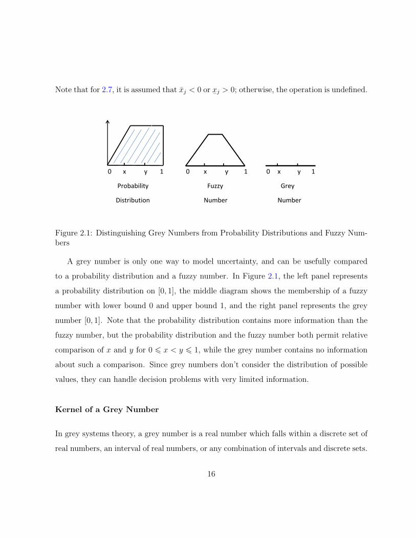
Figure 2.1: Distinguishing Grey Numbers from Probability Distributions and Fuzzy Num-bers

A grey number is only one way to model uncertainty, and can be usefully compared

to a probability distribution and a fuzzy number. In Figure 2.1, the left panel represents

a probability distribution on [0, 1], the middle diagram shows the membership of a fuzzy

number with lower bound 0 and upper bound 1, and the right panel represents the grey

number [0, 1]. Note that the probability distribution contains more information than the

fuzzy number, but the probability distribution and the fuzzy number both permit relative

comparison of x and y for 0 6 x < y 6 1, while the grey number contains no information

about such a comparison. Since grey numbers don’t consider the distribution of possible

values, they can handle decision problems with very limited information.

Kernel of a Grey Number

In grey systems theory, a grey number is a real number which falls within a discrete set of

real numbers, an interval of real numbers, or any combination of intervals and discrete sets.

16

The operation, which can transfer a grey number into a white number is whitenisation.

The kernel of a grey number is a white number, which is most likely to be the real value

of the grey number. Liu and Fang (2006) defined the expected value of a grey number as

its kernel.

Definition 2.4 Let ⊗x be a grey number, the expected value ⊗x is its kernel.

• If ⊗x is a discrete grey number, and ⊗x ∈ x1, x2, ..., xk, xi ∈ R, i = 1, 2, . . . , k and

1 6 k <∞, then (Liu and Fang, 2006)

⊗x =1

k

k∑i=1

xi (2.8)

• If ⊗x is a continuous grey number, and ⊗x ∈ [x−, x], where x−, x ∈ R, x− 6 x, then (Liu

and Fang, 2006)

⊗x =1

2(x− + x) (2.9)

• If ⊗x is a general grey number, and ⊗x ∈k⋃i=1

[x−i, xi], where 1 6 k <∞, x−i, xi ∈ R,

and xi−1 < x−i 6 xi < x−i+1, x− = minix−i, and x = max

ixi, then

⊗x =

1n

n∑i=1

x−i, if x−i = xi for all i = 1, 2, . . . , k

n∑i=1

(xi−xi)(xi+xi

2)

n∑i=1

(xi−xi), otherwise

(2.10)

17

Degree of Greyness

The degree of greyness reflects the understanding of the uncertainty that is involved in a

decision problem. It can represent the vagueness of input data or a range of possible values

to choose from.

Definition 2.5 Let ⊗x be a general grey number, ⊗x =k⋃i

[x−i, xi], and the lower bound

x− = minix−i the upper bound x = max

ixi. The range of the grey number ⊗x is defined in

(Liu and Forrest, 2010; Yang and John, 2012)

u(⊗x) = |x− x| (2.11)

Definition 2.6 Let U be a finite universe of discourse, U ⊆ R and ⊗x ∈ U . u(⊗x) is the

range of grey number ⊗x. The degree of greyness g•(⊗x) of the general grey number ⊗x

is defined as (Liu and Forrest, 2010; Yang and John, 2012):

g•(⊗x) = u(⊗x)/u(U) (2.12)

Note that u(U) = |Umax − Umin|, and Umax, Umin are respectively the lower and upper

bounds of U.

Theorem 2.6.1 0 6 g•(⊗x) 6 1 The degree of greyness ranges from 0 to 1.

Theorem 2.6.2 g•(U) = 1. The degree of greyness for the finite universe of discourse is

always equal to 1.

Theorem 2.6.3 For any discrete grey number ⊗x ∈ x1, x2, ..., xk, when x1 = xk,

g•(⊗x) = 0; for any continuous grey number ⊗x ∈ [x−, x], x− 6 x, when x− = x, g•(⊗x) = 0.

18

It is obvious that when g•(⊗x) = 0, ⊗x is a white number with specific value; when

g•(⊗x) = 1, ⊗x is a black number, and it can be considered as unknown.

Grey Set and Grey Sequence

In the following, D[0, 1]⊗ represents the set of all grey numbers within the interval [0, 1].

The grey number ⊗x may be a continuous grey number ⊗x ∈ [x−, x], a discrete grey number

⊗x ∈ x1, x2, ..., xk or a general grey number ⊗x ∈k⋃i=1

[x−i, xi].

Definition 2.7 Let U be a universal set, and x ∈ U ; if G ⊆ U is such that the character-

istic function value of x with respect to G can be expressed by a grey number ⊗x ∈ D[0, 1]⊗,

then G is a grey set (Yang et al., 2004; Yang and John, 2012)

The characteristic function here is a general expression, and may be expressed by proba-

bility function, membership function, etc (Yang and John, 2012).

Definition 2.8 A decision system contains m alternatives and n criteria. Let Ai, i =

1, 2, · · · ,m and 1 6 m <∞, be the ith alternative, and its values on criterion j is ⊗xi(j),

j = 1, 2, · · · , n and 1 6 n < ∞. The behavioural grey sequence of the alternative ⊗Xi is

denoted as:

⊗Xi = (⊗xi(1),⊗xi(2), · · · ,⊗xi(j), · · · ,⊗xi(n)). (2.13)

here ⊗Xi is a simple form of ⊗X(Ai), and the value ⊗xi(j) may be a white number,

discrete grey number, continuous grey number or general grey number.

In MCDA, ⊗Xi represents the ith alternatives, and ⊗xi(j) denotes performance of the

ith alternatives on the jth criterion. Using grey numbers to reflect the characteristics

19

of the decision system, we can handle input data with quantitative white numbers and

imperfect information with grey numbers. The definition of a grey sequence can represent

uncertainties in a more general way.

2.1.2 Grey Relational Analysis

Grey Relational Analysis (GRA) is a technique that can deal with MCDA problems with

incomplete information. In MCDA, input data with respect to various criteria (usually

conflicting) usually show that the relationship between two alternatives is complex. GRA

treats each alternative as a sequence of data based on criteria, and calculates the grey

relational degree between each alternative and the reference sequence, which is a generated

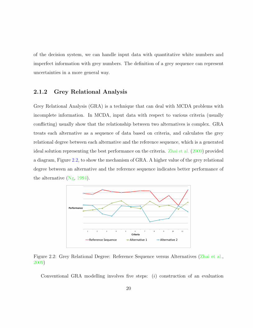
ideal solution representing the best performance on the criteria. Zhai et al. (2009) provided

a diagram, Figure 2.2, to show the mechanism of GRA. A higher value of the grey relational

degree between an alternative and the reference sequence indicates better performance of

the alternative (Ng, 1994).

1 2 3 4 5 6 7 8 9 10 11

Performance

Criteria

Reference Sequence Alternative 1 Alternative 2

Figure 2.2: Grey Relational Degree: Reference Sequence versus Alternatives (Zhai et al.,2009)

Conventional GRA modelling involves five steps: (i) construction of an evaluation

20

structure, (ii) transformation of alternatives into comparability sequences and of the nor-

malized performance matrix, (iii) derivation of reference sequences, (iv) calculation of grey

relational coefficients, (v) determination of the grey relational degree. Explanations and

mathematical expressions of these steps are provided (Chan and Tong, 2007; Liou et al.,

2011; Zhai et al., 2009; Zhang et al., 2011):

Step 1 Construction of an Evaluation Structure: For an MCDA problem, let A =

A1, A2, ...Ai, ..., An be the set of alternatives, and C = C1, C2, ...Cj, ..., Cm be

the set of criteria, where 1 < m,n < ∞. The performance of alternative Ai is

represented as Vi = (Vi1, Vi2, ..., Vij, ..., Vim), where Vij denotes the value of alternative

Ai on criterion Cj. These parameters are represented in Table 2.1.

Table 2.1: Grey Relational Analysis Structure

AlternativesA1 A2 ... Ai ... An

C1

C2 ↓...

Criteria Cj → Vij...Cm

Step 2 Generation of Normalized Performance Matrix: The main objective of nor-

malizing the performance matrix is to transform the alternative Ai = (Vi1, Vi2, ..., Vij,

..., Vim) into a comparability sequence Ai′ = (Vi1

′, Vi2′, ..., Vij

′, ..., Vim′) according to

the three types of criteria: increasing, decreasing, and targeted.

21

• Increasing Criterion: If a larger value of Vij always indicates better performance

of alternative Ai, then

Vij′ =

Vij −minkVkj

maxkVkj −min

kVkj

i = 1, 2, ..., n, j = 1, 2, ...,m

(2.14)

• Decreasing Criterion: If a smaller value of Vij indicates better performance of

alternative Ai, then

Vij′ =

maxkVkj − Vij

maxkVkj −min

kVkj

i = 1, 2, ..., n, j = 1, 2, ...,m

(2.15)

• Targeted Criterion: If a value of Vij closer to the target value Vj∗ indicates

better performance of alternative Ai, then

Vij′ = 1− |Vij − Vj∗|

maxmaxkVkj − Vj∗, Vj∗ −min

kVkj

i = 1, 2, ..., n, j = 1, 2, ...,m

(2.16)

In (2.16), Vj∗ is the target value for the jth criterion, and min

kVkj 6 Vj

∗ 6

maxkVkj.

After the normalization, all three types of criteria have been transformed into in-

creasing criteria, in which a larger value of Vij′ indicates better performance of the

22

alternative. The normalized performance matrix is

V ′ =

V11′ V21

′ ... Vn1′

V12′ V22

′ ... Vn2′

... ... ... ...

V1m′ V2m

′ ... Vnm′

(2.17)

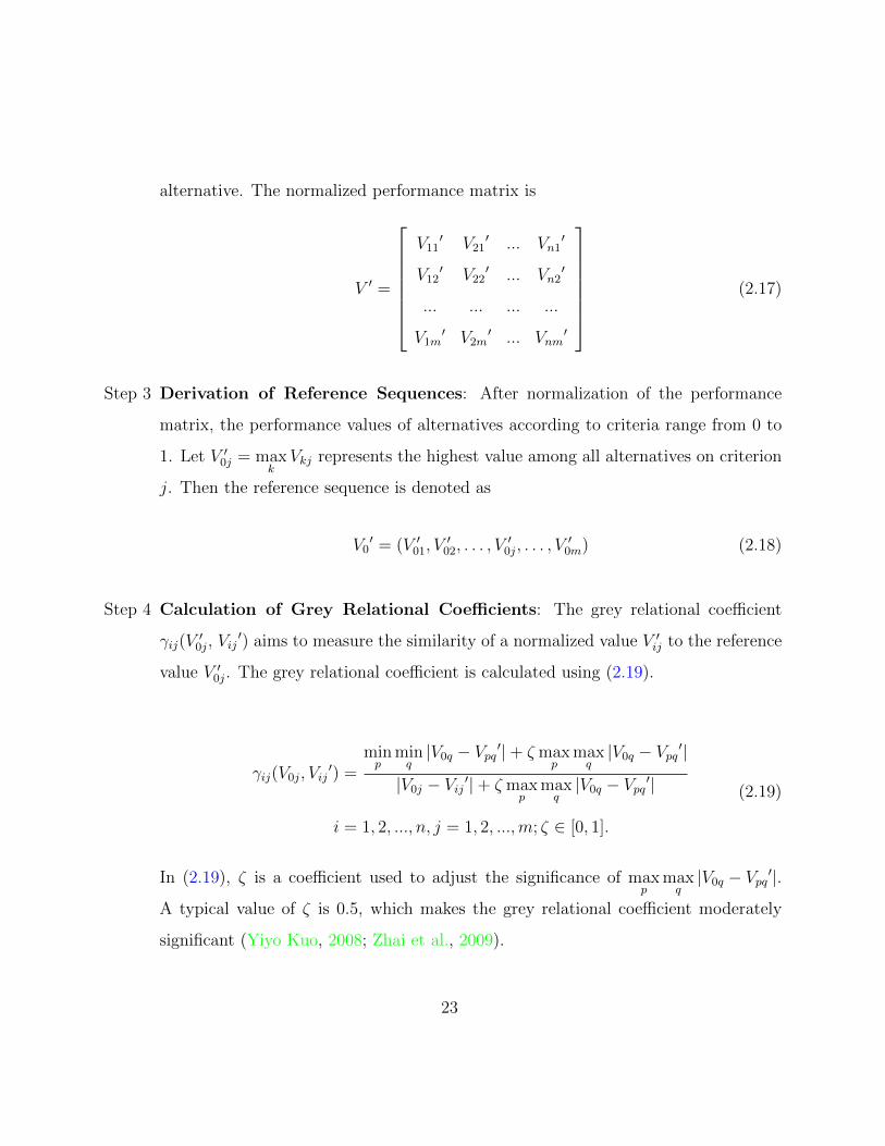
Step 3 Derivation of Reference Sequences: After normalization of the performance

matrix, the performance values of alternatives according to criteria range from 0 to

1. Let V ′0j = maxkVkj represents the highest value among all alternatives on criterion

j. Then the reference sequence is denoted as

V0′ = (V ′01, V

′02, . . . , V

′0j, . . . , V

′0m) (2.18)

Step 4 Calculation of Grey Relational Coefficients: The grey relational coefficient

γij(V′

0j, Vij′) aims to measure the similarity of a normalized value V ′ij to the reference

value V ′0j. The grey relational coefficient is calculated using (2.19).

γij(V0j, Vij′) =

minp

minq|V0q − Vpq ′|+ ζ max

pmaxq|V0q − Vpq ′|

|V0j − Vij ′|+ ζ maxp

maxq|V0q − Vpq ′|

i = 1, 2, ..., n, j = 1, 2, ...,m; ζ ∈ [0, 1].

(2.19)

In (2.19), ζ is a coefficient used to adjust the significance of maxp

maxq|V0q − Vpq ′|.

A typical value of ζ is 0.5, which makes the grey relational coefficient moderately

significant (Yiyo Kuo, 2008; Zhai et al., 2009).

23

Step 5 Determination of Grey Relational Degree: Given all the grey relational coeffi-

cients of normalized values with respect to reference values, the grey relational degree

of an alternative with respect to the reference sequence can be formulated as follows:

γ(A0, Ai) =m∑j=1

wjγ(V0j,V′ij) (2.20)

where wj represents the weight on criteria j, andm∑j=1

wj = 1.

The main objective of grey relational degree is to calculate the magnitude of correla-

tion between alternatives and the reference sequence. Therefore, an alternative with

higher grey relational degree with respect to the reference sequence can be identified

as a better solution.

Grey systems theory is receiving increasing attention in the field of decision making,

and has been successfully applied to many important problems featuring uncertainty. Chan

and Tong (2007) used grey relational analysis in multiple criteria material selection; Li

et al. (2007) developed a grey-based approach to deal with supplier selection; Ozcan et al.

(2011) made a comparison among various multiple criteria decision analysis methods and

grey relational analysis, and then applied grey relational analysis to a warehouse selection

problem; Liou et al. (2011) provided another application aimed at improving airline service

quality. During the last decade, increasing applicability of grey systems theory motivated

many researchers to compare it with related techniques and invent new combinations.

Zhang et al. (2005) investigated grey related analysis using fuzzy interval numbers; Wei

(2011) extended grey systems theory to investigate intuitionistic fuzzy multiple attributes

decision problems; and Tseng (2010) combined linguistic preferences with grey relational

analysis in fuzzy environmental management.

24

2.2 Multiple Criteria Decision Analysis

After more than forty years of development of MCDA, a large variety of methodologies and

technical tools have been developed to assist a DM(s) in solving a decision problem among

a set of alternatives, taking into account multiple criteria. The MCDA methodologies,

mainly focusing on choosing, sorting and ranking problems, can be classified into four

steps (Guitouni and Martel, 1998; Roy, 1991), namely:

• Structure the Decision Situation and Model the Problem. The structure of

the decision problem includes identification of the stakeholders, verification of the

objectives and criteria, specification and selection of the decision alternatives, and

clarification of the problematic.

• Articulate and Model DMs’ Preferences. The preference model must be for-

mulated and validated to ensure that it includes all the relevant information about

the DMs’ preferences.

• Aggregate the Alternative Evaluations in terms of the Criteria. A proper

MCDA technique assesses the alternatives by evaluation and comparison based on the

requirements of the DMs. It is also called Multiple Criteria Aggregation Procedures

(MCAP).

• Formulate a Recommendation and Implement the Solution. Further analysis

may be needed to provide detailed guidance based on the calculation results.

25

2.2.1 Review of MCDA Approaches

MCDA is widely used as an integrated methodology for systematic decision making ac-

cording to multiple criteria. With the rapid development of MCDA, numerous theoretical

and practical advances have been achieved, and significant reviews have been presented by

several researchers: Ozernoy (1992), and Guitouni and Martel (1998) articulated guide-

lines for choosing an appropriate MCDA method in different situations; Steward (1992),

Vincke (1992), Belton and Stewart (2002), and Greco (2004) presented exhaustive re-

views of MCDA approaches, classifying and summarizing classical methods and putting

forward some challenging issues; Dyer et al. (1992) focused on the development of Multiple

Attribute Utility Theory (MAUT), and describing some aspects of MAUT, which they up-

dated 16 years later (Wallenius et al., 2008). All of these works contributed tremendously

to the development of MCDA. Based on the previous reviews, the conventional theoretical

methods in the field of MCDA can be distinguished into three major categories.

• Multiple Objective Optimisation (MOO) Dealing with a decision problem, a

DM may have several objectives that need to be satisfied simultaneously. In this

situation, it may be hard to generate an optimal solution. The main purpose of

MOO is to seek satisfactory, non-dominated options, in another words, to generate

solutions that can provide suitable performance over all objectives for the DM. Goal

programming and evolutionary multiple objective optimisation are well developed in

this field (Charnes and Cooper, 1977; Coello et al., 2007; Marler and Arora, 2004;

Tamiz et al., 1998).

• Value-focused Approaches or Multiple Attribute Utility Theory (MAUT)

Value-focused approaches were put forward by Keeney and Raiffa (1993). These

methods try to assign a marginal utility value to one of a finite set of feasible al-

26

ternatives over each criterion. Then, techniques are developed to aggregate these

marginal utility values. One of the most widely used aggregation approaches is

weighted sum modelling (Dyer et al., 1992). The aggregated utility value of an alter-

native, a real number, represents its relative preference over the other alternatives,

and the alternative with higher utility value is preferred by DMs (Wallenius et al.,

2008). One representative of value-focused approaches is AHP (Analytic Hierarchy

Process), developed by Saaty (1994). This methodology can decompose a decision

problem into a hierarchy of more easily comprehensive sub-problems and use pairwise

comparisons to gather partial preferences of DMs.

• Outranking Methods

The outranking models focus on pairwise comparison of a finite set of alternatives

over multiple criteria. Different from value-focused approaches, the output of these

methods is not a real number, but an outranking relation. A solution here means

that enough arguments can be provided to declare that the option is at least as good

as another (Belton and Stewart, 2002). The ELECTRE and PROMETHEE are

commonly used outranking methodologies (Roy, 1991; Brans and Mareschal, 2005)

Many other aspects of modern MCDA research, and integrations of MCDA methods

with other methodologies need to be mentioned, such as problem structuring techniques

(Mingers and Rosenhead, 2004), criteria aggregation models (Damart et al., 2007; Grabisch

et al., 2003), robustness analysis (Hites et al., 2006), preference modelling and learning

(Furnkranz and Hullermeier, 2011), and integration of MCDA with group decision mak-

ing and negotiation approaches (Belton and Pictet, 1997; Leyva-Lopez and Fernandez-

Gonzalez, 2003; Matsatsinis and Samaras, 2001).

27

Handling uncertainty with reasonable and systematic methodologies has been a promi-

nent topic in MCDA (Zarghami et al., 2011) over the past two decades. At the theoretical

level, there have been many surveys of related techniques, such as Chen et al. (1992)’s

comprehensive survey of fuzzy discrete MCDA methods; Carlsson and Fuller (1996)’s sum-

mary of the development of fuzzy MCDA in the 1990s, focusing on the interdependence of

criteria in MCDM; Greco et al. (1999, 2001)’s proposed MCDA procedures related to rough

set theory; Ian N. Durbach (2012)’s review of technical tools used in uncertain MCDA and

simulation experiment to assess some simplified value function approaches. At the practi-

cal level, practitioners applied these approaches in different fields, especially management

of natural resources, such as forests (Mendoza and Martins, 2006), water resources (Hyde

et al., 2005), and energy (Tylock et al., 2012).

2.2.2 PROMETHEE Modelling

The PROMETHEE (Preference Ranking Organization Method for Enrichment Evalua-

tions), developed by Brans in 1982, is one of the most accepted MCDA methods, and

has attracted much attention from academics and practitioners (Brans and Mareschal,

1995, 2005). A multiple criteria outranking methodology, it assists DMs with different

perspectives to achieve a consensus on feasible alternatives (Hermans and Erickson, 2007;

Machant, 1996), and makes it comparatively easy to rank and prioritize these alternatives

over multiple criteria.

The PROMETHEE II method can provide a complete ranking of alternatives based on

pairwise comparisons, while PROMETHEE can only give partial ranking of alternatives.

Assume that a decision system contains n alternatives A = A1, A2, . . . , An and m eval-

uation criteria C = C1, C2, . . . , Cm for one DM. For Ap, Aq ∈ A, let Vpk and Vqk denote

28

the performance of alternatives Ap and Aq, respectively, on criterion k, and let Pk be the

DM’s selected preference function for criterion k. (For each criterion, six specific preference

functions can be used to calculate the preference degree of one alternative over another

(Brans et al., 1986).) Then, the DM’s preference for alternative Ap over Aq according to

criterion k equals Pk(Vpk − Vqk). After that, let wk represent the DM’s assessment of the

importance of criterion k, wherem∑k=1

wk = 1.

The relative preference of alternative Ap over Aq across criteria is

π(Ap, Aq) =m∑k=1

wkPk(Vpk − Vqk) (2.21)

After that, the outflow of Vp, a measure of the preference of alternative Ap over all other

alternatives, is defined by

φ+(Ap) =1

n− 1

n∑q=1q 6=p

π(Ap, Aq) (2.22)

Similarly, the inflow of Ap, a measure of the extent to which Ap is not as good as other

alternatives, is denoted by

φ−(Ap) =1

n− 1

n∑q=1q 6=p

π(Aq, Ap) (2.23)

The evaluation of the net flow of alternative Ap is obtained by subtracting the inflow from

the outflow. Usually, alternatives with higher values of net flow are ranked higher.

φ(Ap) = φ+(Ap)− φ−(Ap) (2.24)

29

The outranking methods of the PROMETHEE family are realistic and flexible, and can

be used to model and analyze decision problems with multiple criteria. PROMETHEE II,

which provides a complete ranking of a finite set of feasible alternatives, is based on pair-

wise comparisons of alternatives according to each criterion. The criteria may contain

both tangible and intangible information, thereby providing a comprehensive assessment

of performance. However, the relative performance of alternatives on qualitative criteria

evaluated by DMs may be imprecise, arbitrary, or lack consensus, and the input data

on quantitative criteria may be difficult to obtain (Behzadian et al., 2010; Pedrycz et al.,

2011). Hence, uncertainty of input values in the PROMETHEE method must be taken into

account. Le Teno and Mareschal (1998) put forward an interval version of PROMETHEE

method for handling ill-defined information; Goumas and Lygerou (2000) extended the

PROMETHEE method for decision making in the form of fuzzy number; Halouani et al.

(2009) introduced a 2-tuple linguistic representation model dealing with imprecise informa-

tion; Li and Li (2010) extended the PROMETHEE II method based on generalized fuzzy

numbers, to assess the weights of criteria and the ratings of alternatives; and Hyde et al.

(2003) incorporated uncertainty in the PROMETHEE method and proposed a reliability-

based approach.

2.3 Conclusions

This chapter begins by systematically reviewing mathematical concepts of grey systems

theory, such as grey numbers, the kernel of a grey number, the degree of greyness, grey

sets, and grey sequences. A literature review is conducted on methods of grey systems

theory, which have been successfully applied to decision problems. A representative tech-

nique, grey relational analysis, is presented to determine the preferences of alternatives by

30

calculating the magnitude of dependence between alternatives and the reference sequence.

In the following chapters of the thesis, the fundamental concepts and methods of grey sys-

tems theory will be further developed for incorporation into MCDA and GMCR to model

decision analysis under uncertainty.

After that, a variety of methodologies and techniques, dealing with choosing, sorting

and ranking alternatives in MCDA are summarized and classified. In addition, systematic

methodologies for handling uncertainty problems in the field of MCDA over the past two

decades are reviewed, and some informative surveys of MCDA techniques are pointed out

for further reading. Moreover, a multiple criteria outranking methodology, PROMETHEE

II is reviewed, and its theoretical calculation process is discussed. This method will be

developed and modified in the following chapter to handle decision problems having both

quantitative and qualitative criteria and uncertain information through the integration of

grey techniques.

31

Chapter 3

The Grey-based PROMETHEE II

Methodology

3.1 Introduction

The main objective of this chapter is to incorporate grey numbers into Preference Ranking

Organization METHod for Enrichment Evaluation II (PROMETHEE II), a multiple crite-

ria outranking methodology. This methodology assists DMs with different perspectives to

achieve a consensus on alternatives ranked according to both qualitative and quantitative

criteria under uncertainty. This approach uses the concept of grey numbers to represent

information that is uncertain or ill-defined, and then combines it with PROMETHEE II.

The grey-based PROMETHEE II methodology can produce results that consider the un-

certainties associated with vague input data. To help accomplish this objective, this chap-

ter presents the notation, definitions and detailed calculation processes of the grey-based

PROMETHEE II methodology. The feasibility and usefulness of the proposed methodol-

32

ogy is demonstrated using an illustrative case study.

Multiple Criteria Decision Analysis

Normalized Grey Performance Matrix

Normalized Performance on

Qualitative Criteria

Relations between Linguistic expressions

with Grey Interval Numbers

Quantitative Criteria

Qualitative Criteria

Normalized Performance on

Quantitative Criteria

Alternative ranking

Relative Preference Measurements for Performance Measures

Netflows of Alternatives

Criteria Decision MakersAlternatives

Individual Judgment of DMs

Importance Degree of DMs

PROMETHEE II

Figure 3.1: Flow Chart of Grey-based PROMETHEE II Methodology

A framework of the grey-based PROMETHEE II methodology is displayed in Figure

3.1. The decision analysis process depends on three main procedures:

• Problem structuring for MCDA with uncertain information. As can be seen near

the top of Figure 3.1, the structure contains three main parts: multiple alternatives,

criteria and DMs.

• Normalizing the performance of alternatives on multiple criteria. The criteria are

33

further classified as quantitative or qualitative. Two techniques are employed to

normalize the performance of alternatives on these two types of criteria. For quan-

titative criteria, uncertain input data is used to measure the performance of alter-

natives; for qualitative criteria, individual judgements of DMs, represented using

linguistic expressions are collected to access the performance of alternatives. After

the normalization, a grey performance matrix is generated.

• Ranking alternatives based on the PROMETHEE II methodology. In this research,

as one of the main contributions, a relative preference evaluation method is used

to measure the preference degree of one alternative over another. This method is

incorporated into PROMETHEE II to generate a complete ranking of the alternatives

with uncertain information.

3.2 Grey-based PROMETHEE II Methodology

3.2.1 Structure of the Grey Decision System

The main purpose of grey-based PROMETHEE II is to rank alternatives, A = A1, A2, . . . ,

An, by DMs, DM = DM1, DM2, . . . , DML, according to criteria, C = C1, C2, . . . ,

Cm. The decision structure is based mainly on a grey description function and a grey

decision system (Kuang et al., 2014d).

Definition 3.1 Let A×C be the Cartesian Product of the set of alternatives A and the set

of criteria C, and let G[R] denote the set of all grey numbers. A grey description function

f⊗ : A× C → G[R] (3.1)

34

describes the performance values of the alternatives on the criteria. For example, for

Ai ∈ A and Cj ∈ C, f⊗(Ai, Cj) = ⊗Vij is a grey number representing performance of

alternative Ai on criterion Cj.

Definition 3.2 Let A = A1, A2, . . . , An be a set of n alternatives, C = C1, C2, . . . , Cm

be a set of m criteria, DM = DM1, DM2, . . . , DML be a decision group that contains

L DMs, and let f⊗ : A × C → G[R] denote a grey description function. A grey decision

system is defined as

GE = (A,C,DM, f⊗) (3.2)

The decision structure is usually represented using a performance matrix having alterna-

tives as columns, criteria as rows, and performance of alternatives on criteria as the matrix

entries. Given a grey description function f⊗ : A X C → G[R], the performance of the al-

ternative Ai ∈ A on the criterion Cj ∈ C is denoted as ⊗Vij = f⊗(Ai, Cj). In this approach,

this performance may be an continuous grey number or a white number. Then an MCDA

problem with uncertainty can be represented by Table 3.1. With this representation, each

alternative may be represented as a sequence of performance measurements over the crite-

ria. For example, alternative Ai may be represented as Ai = (⊗Vi1,⊗Vi2, . . . ,⊗Vim).

Table 3.1: Grey-based Decision Structure

Alternatives

A1 A2 . . . Ai . . . AnC1

C2 ↓. . .

Criteria Cj → ⊗Vij. . .

Cm

35

3.2.2 Normalizing the Performance of Alternatives

The criteria in a decision problem may be either quantitative or qualitative. This section

aims to determine the performance of alternatives according to both types of criteria, and

normalize their performance.

This approach considers multiple DMs and is designed to improve the group decision

process. When multiple DMs are involved in decision processes, the importance of each DM

may be unequal, and sometimes it is necessary to assign different degrees of importance

to DMs. In order to determine the importance of each DM in a group decision, French Jr

(1956) considered the power relations among members of the group, Keeney and Raiffa

(1976) suggested interpersonal comparisons of preferences, and Bodily (1979) introduced

a delegation process for setting the weights for DMs. In the proposed methodology, the

weight of each DM is voted by the other DMs according to importance, expressed with

linguistic information. Then, DMs express their preferences of alternatives based on each

qualitative criterion. Both the weights and the preferences are transformed to continuous

grey numbers. Note that the performance of alternatives on quantitative criteria is ex-

pressed in terms of measured numeric values, which do not depend on DMs’ opinions. The

normalization measurements of alternatives based on quantitative and qualitative criteria

are introduced separately

Quantitative criteria

Quantitative performance measurements can be normalized according to three forms of

criteria: increasing, decreasing and targeted. Let ⊗Viq, i = 1, 2, . . . , n, denote numeri-

cal values of alternative i on quantitative criterion q, and let V− iq and V iq represent the

lower bound and the upper bound of ⊗Viq, respectively. The normalized performance of

36

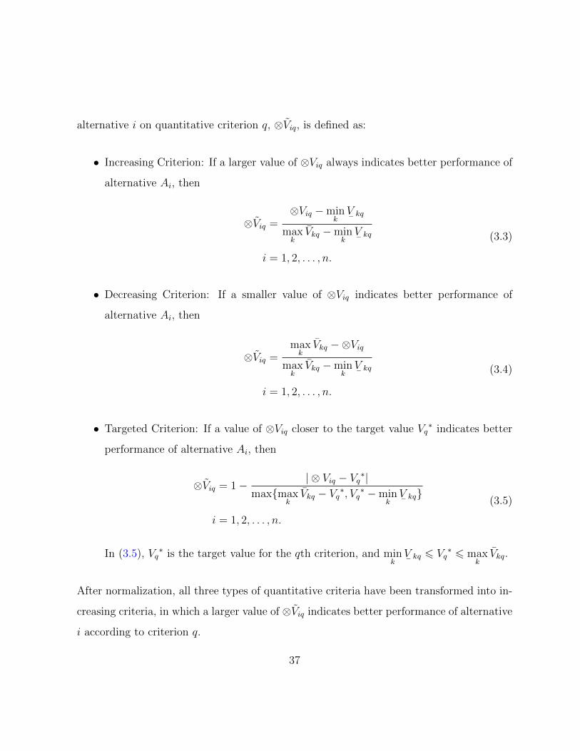
alternative i on quantitative criterion q, ⊗Viq, is defined as:

• Increasing Criterion: If a larger value of ⊗Viq always indicates better performance of

alternative Ai, then

⊗Viq =⊗Viq −min

kV− kq

maxkVkq −min

kV− kq

i = 1, 2, . . . , n.

(3.3)

• Decreasing Criterion: If a smaller value of ⊗Viq indicates better performance of

alternative Ai, then

⊗Viq =maxkVkq −⊗Viq

maxkVkq −min

kV− kq

i = 1, 2, . . . , n.

(3.4)

• Targeted Criterion: If a value of ⊗Viq closer to the target value Vq∗ indicates better

performance of alternative Ai, then

⊗Viq = 1− | ⊗ Viq − Vq∗|maxmax

kVkq − Vq∗, Vq∗ −min

kV− kq

i = 1, 2, . . . , n.

(3.5)

In (3.5), Vq∗ is the target value for the qth criterion, and min

kV− kq 6 Vq

∗ 6 maxkVkq.

After normalization, all three types of quantitative criteria have been transformed into in-

creasing criteria, in which a larger value of ⊗Viq indicates better performance of alternative

i according to criterion q.

37

Qualitative criteria

Multiple DMs are considered within a group decision making concept. Different weights

are assigned to DMs according to their importance, and linguistic expressions are utilized

to represent both the importance of each DM and the performance of alternatives. The

performance of alternatives on qualitative criteria is evaluated by DMs, and each DM

has his or her own grey-based performance matrix. Qualitative performance measure-

ments should be suitably designed based on increasing criterion, insofar as possible, so

that individual judgements of DMs on an alternative can be aggregated according to their

importance. Then, one overall matrix reflecting the preferences of all the DMs is produced,

and the aggregated matrix is normalized to make the maximum upper bound equal to one.

In particular, qualitative performance measurements can be normalized according to the

following procedures:

(1) Normalize the importance degree assigned to each DM.

Definition 3.3 Let L represent the number of DMs, and ⊗dl denote the importance degree

of DM l. Then, the normalized importance degree of DM l is

⊗ dl =⊗dl∑

i=1

⊗di(3.6)

(2) Evaluate the performance of the alternatives for each DM. Let ⊗V lip represent the

performance of alternative i on qualitative criterion p given by DM l. The grey-based

performance matrix for DM l over qualitative criteria is shown in Table 3.2.

38

Table 3.2: Grey-based Performance Matrix by DM l on Qualitative Criteria

DM l Alternatives

A1 A2 ... Ai ... An... ... ... ... ... ... ...

Criteria Cp ⊗V l1p ⊗V l

2p ... ⊗V lip ... ⊗V l

np

... ... ... ... ... ... ...

(3) Aggregate the performance of alternatives based on qualitative criteria for all deci-

sion makers.

Definition 3.4 Let ⊗V lip represent the performance of alternative i on qualitative criterion

p evaluated by DM l, and ⊗dl denote the normalized importance degree of DM l. The

aggregated performance of alternative i on qualitative criterion p for all DMs is

⊗ Vip = [⊗d1 ×⊗V 1ip +⊗d2 ×⊗V 2

ip + ...+⊗dL ×⊗V Lip ] (3.7)

Note that, in (3.6) and (3.7), there are relationships to map linguistic expressions into

grey numbers. In a linguistic approach, the linguistic expressions are used for DMs to

express their judgements on alternatives. The linguistic term set can be determined based

on the uncertainty degree and a DM’s preferences. In a decision process, DMs may respond

differently to the same decision context and different linguistic term sets may be chosen

by DMs to evaluate the performance of alternatives over qualitative criteria (Chen, 2011;

Herrera et al., 2000). This approach allows DMs to use multi-granular linguistic term sets

for expressing the linguistic performance of alternatives, and assigning different sets of grey

numbers to linguistic information according to DMs’ preferences. Therefore, the DMs can

39

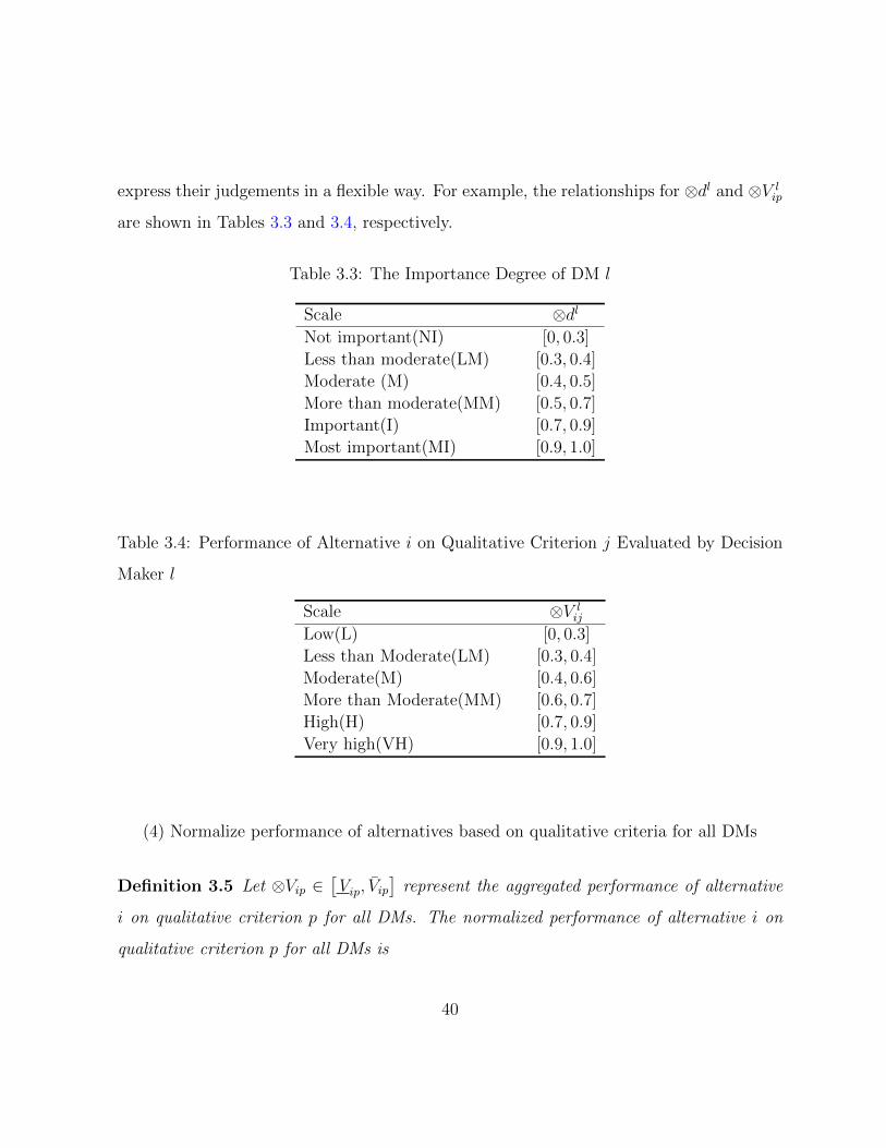
express their judgements in a flexible way. For example, the relationships for ⊗dl and ⊗V lip

are shown in Tables 3.3 and 3.4, respectively.

Table 3.3: The Importance Degree of DM l

Scale ⊗dlNot important(NI) [0, 0.3]

Less than moderate(LM) [0.3, 0.4]

Moderate (M) [0.4, 0.5]

More than moderate(MM) [0.5, 0.7]

Important(I) [0.7, 0.9]

Most important(MI) [0.9, 1.0]

Table 3.4: Performance of Alternative i on Qualitative Criterion j Evaluated by Decision

Maker l

Scale ⊗V lij

Low(L) [0, 0.3]

Less than Moderate(LM) [0.3, 0.4]

Moderate(M) [0.4, 0.6]

More than Moderate(MM) [0.6, 0.7]

High(H) [0.7, 0.9]

Very high(VH) [0.9, 1.0]

(4) Normalize performance of alternatives based on qualitative criteria for all DMs

Definition 3.5 Let ⊗Vip ∈[Vip, Vip

]represent the aggregated performance of alternative

i on qualitative criterion p for all DMs. The normalized performance of alternative i on

qualitative criterion p for all DMs is

40

⊗ Vip =⊗Vip

maxkVkp

(3.8)

Normalized performance of alternatives

After completing the above calculation processes, a normalized performance matrix of

alternatives according to criteria can be generated as shown in (3.9), which aggregates the

information of importance degree of DMs, the individual judgement of DMs on performance

of alternatives on qualitative criteria, and the performance of alternatives on quantitative

criteria.

⊗ V =

⊗V11 ⊗V21 ... ⊗Vn1

⊗V12 ⊗V22 ... ⊗Vn2

... ... ... ...

⊗V1m ⊗V2m ... ⊗Vnm

(3.9)

The normalized performance matrix reflects the performance of alternatives on three

types of quantitative criteria and viewpoints of all the DMs according to qualitative criteria.

It is used as input to an MCDA decision rule for ranking alternatives in group decision

making, and PROMETHEE II, a flexible methodology, is further discussed and modified

for accomplishing this ranking.

41

3.2.3 Ranking Alternatives based on PROMETHEE II

Methodology

In this section, alternatives are compared in pairs on each criterion. Since performance of

alternatives according to criteria may be represented by continuous grey numbers, a new

preference function is designed to measure the degree to which one alternative is preferred

to another. A multiple criteria preference index is calculated based on the comparison

of each pair of alternatives. According to the PROMETHEE II outranking method, the

inflow, outflow, and net flow for each alternative are determined separately.

Let two continuous grey numbers ⊗Vaj = [V− aj, Vaj] and ⊗Vbj = [V− bj, Vbj] represent the

performance of alternatives Aa and Ab, respectively, according to criterion j. In particular,

when ⊗Vaj = V− aj = Vaj = Vaj and ⊗Vbj = V− bj = Vbj = Vbj, they represent two white

numbers with crisp values.

Definition 3.6 The deviation of the performance of alternatives Aa from Ab on criterion

j is defined by Xu and Da (2002).

dj(Aa, Ab) =Vaj − V− bj∣∣∣Vaj − V− aj∣∣∣+

∣∣∣Vbj − V− bj∣∣∣ (3.10)

Thus, dj(Aa, Ab) measures how much the performance of Aa differs from the performance

of Ab on criterion j.

Definition 3.7 If at least one of ⊗Vaj and ⊗Vbj is not a white number, the preference

42

degree of alternative Aa over Ab on criterion j is defined by

Pj(Aa, Ab) = ...

0, if dj(Aa, Ab) 6 0

dj(Aa, Ab), if 0 < dj(Aa, Ab) < 1

1, if dj(Aa, Ab) > 1

(3.11)

From the Definition 3.7, it is clear that Pj(Aa, Ab) is a crisp value and ranges from 0 (no

preference) to 1 (strict preference). The preference degree of alternative a over alternative

b is interpreted as follows, and shown in Figure 3.2.

If Pj(Aa, Ab) = 0, then the performance of alternative Ab is strictly preferred to the

performance of Aa according to criterion j;

If Pj(Aa, Ab) ∈ (0, 0.5), then the performance of alternative Aa is less likely to be

preferred to Ab according to criterion j;

If Pj(Aa, Ab) = 0.5, then the performance of alternatives Aa and Ab is indifferent

according to criterion j;

If Pj(Aa, Ab) ∈ (0.5, 1), then the performance of alternative Aa is more likely to be

preferred to the performance of Ab according to criterion j;

If Pj(Aa, Ab) = 1, then the performance of alternative Aa is strictly preferred to the

performance of Ab according to criterion j.

43

Alternative Aa

Alternative Ab Ab is strictly preferred to Aa

Alternative Aa

Alternative Ab Aa is less likely to be preferred to Ab

Alternative Aa

Alternative Ab Aa and Ab are equally preferred

Alternative Aa

Alternative Ab Aa is more likely to be preferred to Ab

Alternative Aa

Alternative Ab Ab is strictly preferred to Aa

1

Figure 3.2: The Preference Degree of Alternative a over Alternative b

Definition 3.8 If both the grey numbers, ⊗Vaj and ⊗Vbj, are white numbers with crisp

values, written as Vaj and Vbj respectively, the preference degree of Aa over Ab is defined

by

Pj(Aa, Ab) = ...

0, if Vaj < Vbj

0.5, if Vaj = Vbj

1, if Vaj > Vbj

(3.12)

This is a special case of the comparison of two continuous grey numbers. The values

0, 0.5 and 1 represent not preferred, indifferent, and strictly preferred of Aa over Ab on

criterion j, respectively.

It is assumed that DMs can assign weights to all criteria, especially when the number

of criteria is not too large. The weights for the criteria considered here are additive. For

instance, if w1, w2, . . . , wm represent the weights of criteria C1, C2, . . . , Cm respectively,

44

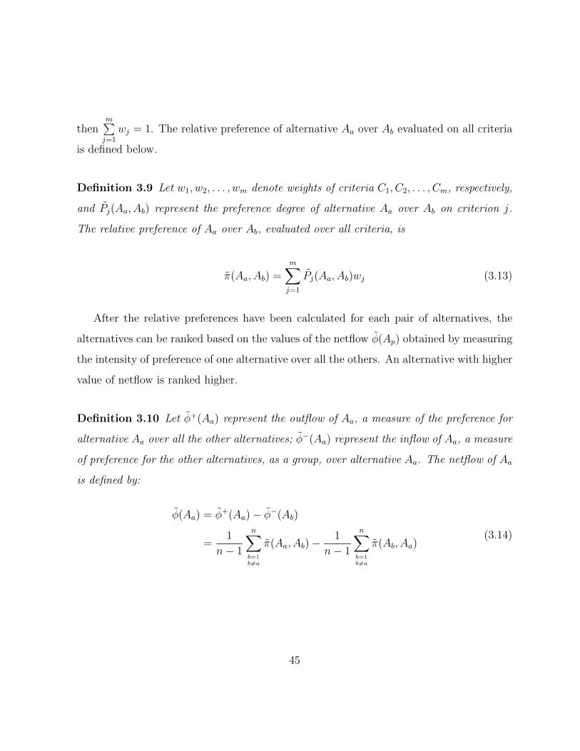
thenm∑j=1

wj = 1. The relative preference of alternative Aa over Ab evaluated on all criteria

is defined below.

Definition 3.9 Let w1, w2, . . . , wm denote weights of criteria C1, C2, . . . , Cm, respectively,

and Pj(Aa, Ab) represent the preference degree of alternative Aa over Ab on criterion j.

The relative preference of Aa over Ab, evaluated over all criteria, is

π(Aa, Ab) =m∑j=1

Pj(Aa, Ab)wj (3.13)

After the relative preferences have been calculated for each pair of alternatives, the

alternatives can be ranked based on the values of the netflow φ(Ap) obtained by measuring

the intensity of preference of one alternative over all the others. An alternative with higher

value of netflow is ranked higher.

Definition 3.10 Let φ+(Aa) represent the outflow of Aa, a measure of the preference for

alternative Aa over all the other alternatives; φ−(Aa) represent the inflow of Aa, a measure

of preference for the other alternatives, as a group, over alternative Aa. The netflow of Aa

is defined by:

φ(Aa) = φ+(Aa)− φ−(Ab)

=1

n− 1

n∑b=1b 6=a

π(Aa, Ab)−1

n− 1

n∑b=1b 6=a

π(Ab, Aa)(3.14)

45

3.3 Case illustration of Evaluation of Source Water

Protection Strategies

In this section, the preference function for measuring preferences of alternative represented

by grey numbers and the proposed grey-based PROMETHEE II method are used for

analyzing the case study in order to rank the alternatives.

3.3.1 Background

As an issue, source water protection is gaining increasing global attention, along with

economic development, population growth and water scarcity (Patrick, 2011). Responding

to the challenges having access to safe drinking water, many projects have been conducted

for ensuring water quality, remediating water contamination, and minimizing potential

threats to surface and groundwater resources (Ferreyra, 2012; Emelko et al., 2011; Qin

et al., 2009).

The Regional Municipality of Waterloo, located in the southwestern part of Ontario,

Canada, is comprised of Kitchener, Waterloo, and Cambridge, as well as adjacent town-

ships. The residents in Waterloo Region access to their drinking water from three main

sources: (i) almost 69 percent is from groundwater through more than 100 municipal

wells; (ii) 28 percent comes from the Grand River; and (iii) the last 3 percent is from the

Great Lakes. In developing its long-term water strategy of ensuring that citizens can enjoy

plentiful and clean drinking water, the Regional Municipality of Waterloo received various

proposals. Therefore, a scientific evaluation system needs to be designed to prioritize or

rank these strategies. The case study is sourced from a technical report entitled “Regional

Municipality of Waterloo Long Term Water Strategy—Phase 1 Report”. The data in this

46

research was simulated, in a manner that is consistent with this report, to demonstrate

the feasibility of this methodology for the MCDA problem having uncertain information

(Regional Municipality of Waterloo and Water Services Division, 1994; Region of Waterloo,

2000).

Since 1993, a number of strategies have been successfully conducted by the Regional

Municipality of Waterloo to implement source water protection for its water supply system

(Region of Waterloo, 2008), and eight strategies have been selected as alternatives for this

case study (Kuang et al., 2012):

• Alternative 1 (A-1): Installation of sentry wells or off-site monitoring wells

• Alternative 2 (A-2): Strategic land purchase and/or easement

• Alternative 3 (A-3): Chemical restriction by municipal law

• Alternative 4 (A-4): Buy-back of contaminated or at-risk land

• Alternative 5 (A-5): Regulation of bulk fuel, retail and accessory use of gasoline

• Alternative 6 (A-6): Replacement of underground diesel fuel storage tanks with above

ground tanks and containment units

• Alternative 7 (A-7): Smart salt project

• Alternative 8 (A-8): Decommissioning and upgrading of wells

With the purpose of providing an overall evaluation on performance of alternatives, this

evaluation system must take account of various kinds of criteria from different perspective,

such as economic development, political and social influence, and ecological maintenance.

47

Four criteria are proposed to evaluate possible alternatives. The meaning of the criteria

are explained in details as follows (Chen et al., 2007; Rajabi et al., 2001):

• INVEST: project investment cost (millions of dollars);

• OPER: projection operating cost (millions of dollars) ;

• RISKD: the alternative’s ability to decrease water quantity and quality risks to water

resources from historical, existing or future practices (Region of Waterloo, Jan, 2008);

• FEAS: technical, operational, law and public feasibility (Rajabi et al., 2001).

Note that INVEST and OPER are quantitative criteria, while RISKD and FEAS are

qualitative criteria.

3.3.2 Input Data

Assume that the illustrative case contains three DMs, DM1, DM2 and DM3. The simu-

lated input data includes importance degrees of DMs, weights of criteria, performance of

source water protection strategies on qualitative criteria, and performance of source water

protection strategies on quantitative criteria, as shown in Tables 3.5-3.8

Table 3.5: Importance Degrees of Decision Makers

DMs DM 1 DM 2 DM 3

Importance Degrees of DMs MM MI I

48

Note that the maps between linguistic expressions and grey numbers are provided in Tables

3.3 and 3.4 on page 40.

Table 3.6: Weights of Criteria

Criteria RISKD FEAS INVEST OPER

Weights 0.3 0.2 0.3 0.2

Table 3.7: Performance of Source Water Protection Strategies on Qualitative Criteria

DM 1 DM 2 DM 3

RISKD FEAS RISKD FEAS RISKD FEAS

A-1 H VH MM VH H H

A-2 VH M H LM H H

A-3 MM H M VH H VH

A-4 H VH H H MM H

A-5 VH H VH H H VH

A-6 H MM VH VH VH LM

A-7 LM VH M H M LM

A-8 H H LM MM M MM

49

Table 3.8: Performance of Source Water Protection Strategies on Quantitative Criteria

Alternatives A-1 A-2 A-3 A-4 A-5 A-6 A-7 A-8

INVEST [14,20] 35 [8,15] 25 3 12 10 [18,23]

OPER [4,7] 1 [4,7] 0.5 15 14 6 [5,7]

3.3.3 Normalization of the Performance of Alternatives

According to the input data listed above, the performance of alternatives over both quan-

titative and qualitative criteria can be normalized.

• For quantitative criteria: INVEST and OPER are decreasing criteria that can be

normalized based on (3.4), and the results are shown in Table 3.10.

• For qualitative criteria: The normalized importance degrees of DMs can be calculated

based on (3.6), and the normalized performance of alternatives over RISKD FEAS can

be generated based on (3.8). The results are shown in Tables 3.9 and 3.10. Note that

the process of normalization depends on the addition and division of grey numbers

given in (2.4) and (2.7), respectively, and creates some overlap of the normalized

importance degrees of the DMs.

Table 3.9: Normalized Importance Degrees of Decision Makers

DMs DM 1 DM 2 DM 3

Importance Degrees of DMs [0.5− 0.7] [0.9− 1.0] [0.7− 0.9]

Normalized Importance Degrees of DMs [0.19− 0.33] [0.35− 0.39] [0.27− 0.43]

50

Table 3.10: Normalized Performance of Alternatives on Criteria

Criteria INVEST OPER RISKD FEAS

Alternative 1 [0.47,0.66] [0.55,0.76] [0.48,0.86] [0.60,0.99]

Alternative 2 0 0.97 [0.54,0.96] [0.33,0.66]

Alternative 3 [0.63,0.84] [0.55,0.76] [0.40,0.76] [0.62,0.1]

Alternative 4 0.31 1 [0.48,0.85] [0.54,0.96]

Alternative 5 1 0 [0.60,0.99] [0.56,0.97]

Alternative 6 0.72 0.14 [0.62,1] [0.46,0.71]

Alternative 7 0.78 0.62 [0.27,0.56] [0.44,0.76]

Alternative 8 [0.38,0.53] [0.55,0.69] [0.31,0.64] [0.45,0.78]

3.3.4 Results and Analysis

Based on the input data and normalized performance of alternatives, a pairwise compar-

ison of all strategies is conducted according to each criterion. Then, a multiple criteria

preference matrix based on the comparison of each pair of source water protection strate-

gies over the criteria of RISKD, FEAS, INVEST, and OPERI is formed according to the

designed preference function, see (3.10-3.12). The results are shown in Table 3.11

51

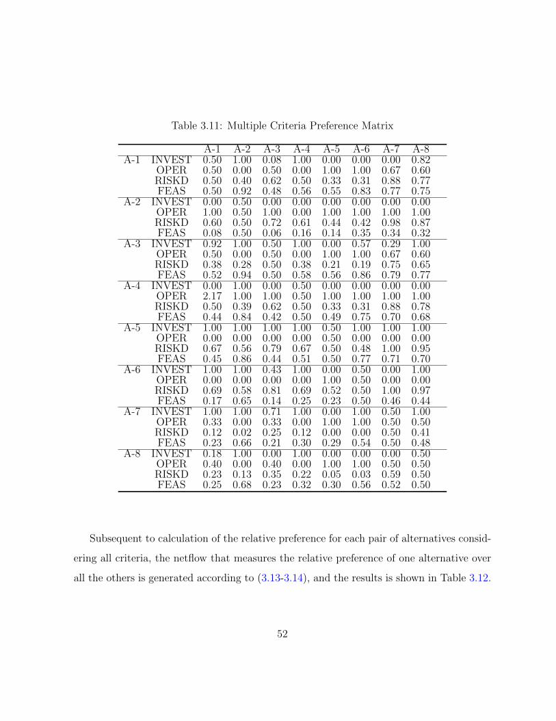
Table 3.11: Multiple Criteria Preference Matrix

A-1 A-2 A-3 A-4 A-5 A-6 A-7 A-8A-1 INVEST 0.50 1.00 0.08 1.00 0.00 0.00 0.00 0.82

OPER 0.50 0.00 0.50 0.00 1.00 1.00 0.67 0.60RISKD 0.50 0.40 0.62 0.50 0.33 0.31 0.88 0.77FEAS 0.50 0.92 0.48 0.56 0.55 0.83 0.77 0.75

A-2 INVEST 0.00 0.50 0.00 0.00 0.00 0.00 0.00 0.00OPER 1.00 0.50 1.00 0.00 1.00 1.00 1.00 1.00RISKD 0.60 0.50 0.72 0.61 0.44 0.42 0.98 0.87FEAS 0.08 0.50 0.06 0.16 0.14 0.35 0.34 0.32

A-3 INVEST 0.92 1.00 0.50 1.00 0.00 0.57 0.29 1.00OPER 0.50 0.00 0.50 0.00 1.00 1.00 0.67 0.60RISKD 0.38 0.28 0.50 0.38 0.21 0.19 0.75 0.65FEAS 0.52 0.94 0.50 0.58 0.56 0.86 0.79 0.77

A-4 INVEST 0.00 1.00 0.00 0.50 0.00 0.00 0.00 0.00OPER 2.17 1.00 1.00 0.50 1.00 1.00 1.00 1.00RISKD 0.50 0.39 0.62 0.50 0.33 0.31 0.88 0.78FEAS 0.44 0.84 0.42 0.50 0.49 0.75 0.70 0.68

A-5 INVEST 1.00 1.00 1.00 1.00 0.50 1.00 1.00 1.00OPER 0.00 0.00 0.00 0.00 0.50 0.00 0.00 0.00RISKD 0.67 0.56 0.79 0.67 0.50 0.48 1.00 0.95FEAS 0.45 0.86 0.44 0.51 0.50 0.77 0.71 0.70

A-6 INVEST 1.00 1.00 0.43 1.00 0.00 0.50 0.00 1.00OPER 0.00 0.00 0.00 0.00 1.00 0.50 0.00 0.00RISKD 0.69 0.58 0.81 0.69 0.52 0.50 1.00 0.97FEAS 0.17 0.65 0.14 0.25 0.23 0.50 0.46 0.44

A-7 INVEST 1.00 1.00 0.71 1.00 0.00 1.00 0.50 1.00OPER 0.33 0.00 0.33 0.00 1.00 1.00 0.50 0.50RISKD 0.12 0.02 0.25 0.12 0.00 0.00 0.50 0.41FEAS 0.23 0.66 0.21 0.30 0.29 0.54 0.50 0.48

A-8 INVEST 0.18 1.00 0.00 1.00 0.00 0.00 0.00 0.50OPER 0.40 0.00 0.40 0.00 1.00 1.00 0.50 0.50RISKD 0.23 0.13 0.35 0.22 0.05 0.03 0.59 0.50FEAS 0.25 0.68 0.23 0.32 0.30 0.56 0.52 0.50

Subsequent to calculation of the relative preference for each pair of alternatives consid-

ering all criteria, the netflow that measures the relative preference of one alternative over

all the others is generated according to (3.13-3.14), and the results is shown in Table 3.12.

52

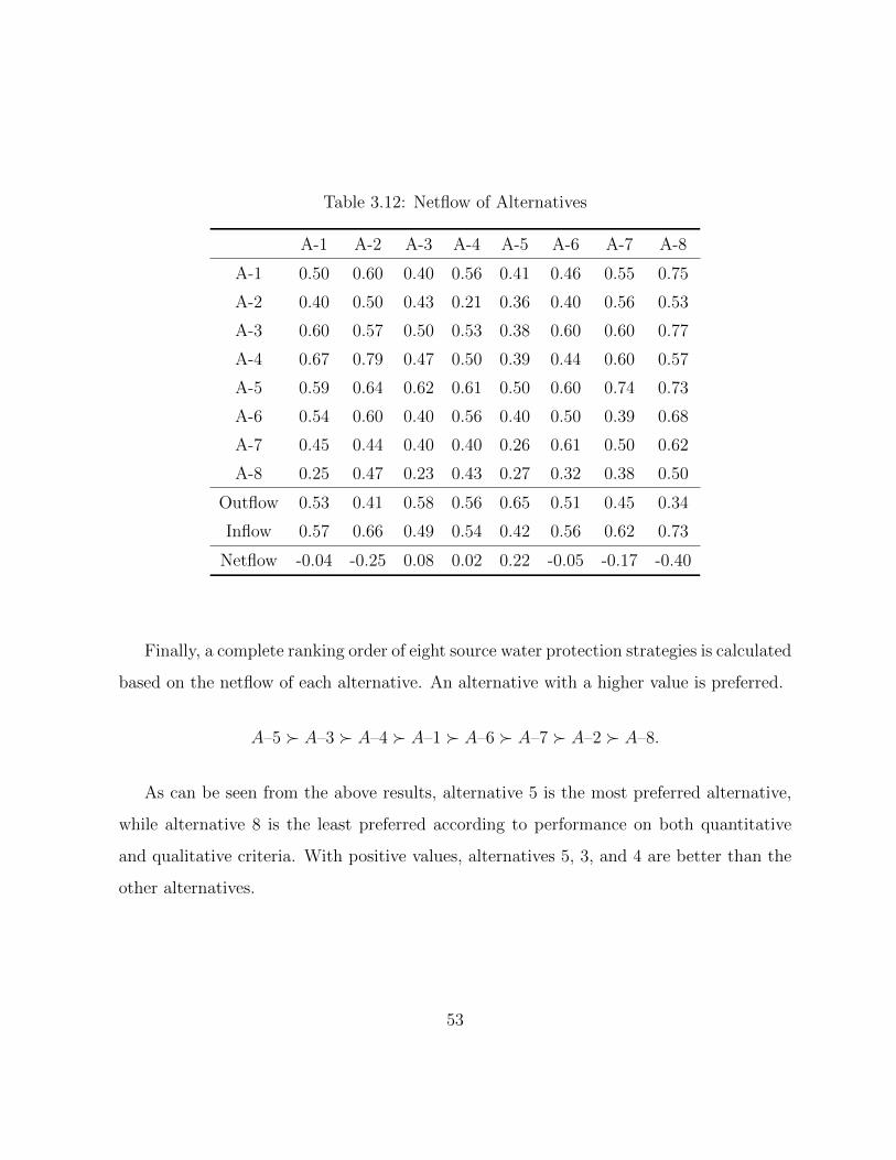
Table 3.12: Netflow of Alternatives

A-1 A-2 A-3 A-4 A-5 A-6 A-7 A-8

A-1 0.50 0.60 0.40 0.56 0.41 0.46 0.55 0.75

A-2 0.40 0.50 0.43 0.21 0.36 0.40 0.56 0.53

A-3 0.60 0.57 0.50 0.53 0.38 0.60 0.60 0.77

A-4 0.67 0.79 0.47 0.50 0.39 0.44 0.60 0.57

A-5 0.59 0.64 0.62 0.61 0.50 0.60 0.74 0.73

A-6 0.54 0.60 0.40 0.56 0.40 0.50 0.39 0.68

A-7 0.45 0.44 0.40 0.40 0.26 0.61 0.50 0.62

A-8 0.25 0.47 0.23 0.43 0.27 0.32 0.38 0.50

Outflow 0.53 0.41 0.58 0.56 0.65 0.51 0.45 0.34

Inflow 0.57 0.66 0.49 0.54 0.42 0.56 0.62 0.73

Netflow -0.04 -0.25 0.08 0.02 0.22 -0.05 -0.17 -0.40

Finally, a complete ranking order of eight source water protection strategies is calculated

based on the netflow of each alternative. An alternative with a higher value is preferred.

A–5 A–3 A–4 A–1 A–6 A–7 A–2 A–8.

As can be seen from the above results, alternative 5 is the most preferred alternative,

while alternative 8 is the least preferred according to performance on both quantitative

and qualitative criteria. With positive values, alternatives 5, 3, and 4 are better than the

other alternatives.

53

3.4 Conclusions

The proposed methodology extends the PROMETHEE II method to deal with ill-defined

information. A performance matrix is defined for evaluating alternatives, according to

both quantitative and qualitative criteria, across all DMs. Uncertainty of input values

in the PROMETHEE II method is taken into account, and continuous grey numbers are

integrated with linguistic expressions to represent both the importance degree of each DM

and the performance of alternatives.

Detailed calculation procedures for normalization are provided. The quantitative per-

formance measurements are normalized based on three types of criteria: increasing, de-

creasing and targeted. As performance data for alternatives may be uncertain, this method

allows continuous grey numbers to represent the input data. The qualitative performance

measurements are taken into account in the group decision, and mutual voting is used to

assign different weights to DMs according to their importance. The performance of alter-

natives is separately evaluated by each DM and, finally, individual judgements of all DMs

are aggregated and normalized.

As the normalized performance matrix contains uncertain information represented by

continuous grey numbers, a new preference function is developed for PROMETHEE II to

compare alternatives in a pairwise fashion on each criterion and, subsequently, to order the

alternatives. This preference function measures the preference degree of one alternative

over another. Compared with the original six types of preference functions, it is more

suitable for application to real cases where input data are similar but not identical.

MCDA methods are designed for handling certain types of decision situations. Com-

pared with other MCDA techniques, the grey-based PROMETHEE II methodology pre-

sented in this chapter can: (i) represent ill-defined information with grey numbers; (ii)

54

simultaneously handle quantitative and qualitative criteria; (iii) incorporate a preference

measurement function into PROMETHEE II; and (iv) deal with multiple criteria and a

group decision through aggregating individual decisions. The numerical case study shows

the suitability of the methodology to handle multi-criteria decisions with uncertain infor-

mation, and illustrates its potential applicability.

55

Chapter 4

The Graph Model for Conflict

Resolution

4.1 Introduction

In this chapter, theoretical definitions of Graph Model for Conflict Resolution (GMCR) are

presented, and solutions concepts (or stability definitions) are provided for carrying out a

stability analysis for a conflict with two or more DMs. After that, this methodology is used

for analyzing a conflict involving water use and oils sands development in the Athabasca

River in Alberta, Canada. In the case study, stable sates are calculated, and strategic

interpretations of the stability results are provided.

The main purpose of the graph model methodology is to describe the key characteristics

of a conflict based on the possible interactions of DMs as dictated by their strategies and

preferences, and then generate the possible compromise resolutions, or equilibria, through

extensive analyses (Hipel et al., 1997). Within the graph model paradigm, a conflict model

56

requires four main components: (i) a set of DMs, (ii) a set of feasible states, (iii) possible

movements between states controlled by each DM, and (iv) each DM’s relative preference

over the feasible states (Fang et al., 1993; Hamouda et al., 2004). In general, if a DM has no

incentive to move from the present state, this state is stable for the DM. If a state is stable

for all DMs, it constitutes an equilibrium of the model. The main stability definitions

included in the graph model are Nash stability (R) (Nash, 1950), general metarationality

(GMR) (Howard, 1971), symmetric metarationality (SMR) (Howard, 1971), and sequential

stability (SEQ) (Fraser and Hipel, 1984). These stability definitions describe possible moves

and countermoves representing common patterns of human behaviours.

4.2 Theoretical Foundations of the Graph Model for

Conflict Resolution

The graph model methodology represents possible scenarios (or states) of a conflict as

vertices of a graph, and the transitions controlled by each DM as the arcs of the graph,

labelled by the DM controlling a given move in one step. Note that, in a graph model,

the movements of DMs can be reversible or irreversible, and no loops are contained in any

DM’s graph. To formally model a conflict, the four fundamental components of GMCR

mentioned above are mathematically expressed as follows (Fang et al., 1993; Hipel et al.,

1997; Kilgour and Hipel, 2005):

• N = 1, 2, . . . , n, n > 2, represents the set of DMs. For the case of two DMs,

N = 1, 2.

• S = s1, s2, . . . , sm, m > 1, denotes the set of feasible states. The particular state

where the conflict begins is designated as the status quo state.

57

• For k ∈ N , Gk = (S,Ak) denotes DM k’s directed graph. Here, Ak ⊆ S × S

represents the set of arcs controlled by DM k. For example, for si, sj ∈ S and

si 6= sj, (si, sj) ∈ Ak if and only if DM k can unilaterally move the conflict from state

si to state sj in one step. In this case, state sj is reachable from state si for DM k.

Then, the collection of the directed graphs of all the DMs, G = (S,Ak), k ∈ N,

can be convincingly used to model the conflict.

• For k ∈ N , a binary relation k,∼k on S expresses DM k’s preference of one state

over another. Specifically, for si, sj ∈ S, si k sj indicates that si is strictly preferred

to sj by DM k, while si ∼k sj means that si is equally preferred to sj.

To formally define the previously mentioned four major stability concepts within the

graph model framework, one needs to identify states that are unilaterally reachable by a

DM. Accordingly, the definitions of reachable list and the unilateral improvement list are

given below (Fang et al., 1993, 2003a; Hipel et al., 1997).

Definition 4.1 The Reachable list for a DM Let k ∈ N and s ∈ S. The reachable

list from state s for DM k is

Rk(s) = si ∈ S : (s, si) ∈ Ak. (4.1)

Note that the reachable list from a given state for a DM represents a collection of all

possible states to which the DM can move in one step.

Definition 4.2 The Unilateral Improvement List for a DM Let k ∈ N and s ∈ S.

The unilateral improvement list from state s for DM k is

R+k (s) = si ∈ Rk(s) : si k s. (4.2)

58

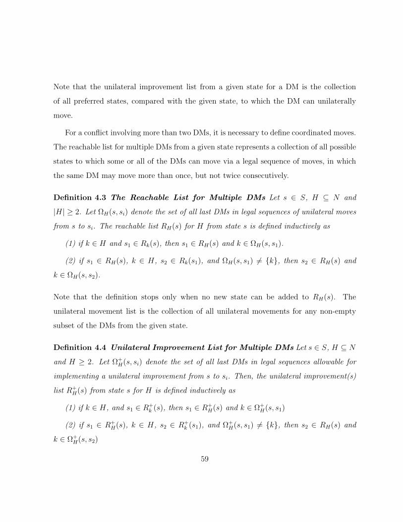
Note that the unilateral improvement list from a given state for a DM is the collection

of all preferred states, compared with the given state, to which the DM can unilaterally

move.

For a conflict involving more than two DMs, it is necessary to define coordinated moves.

The reachable list for multiple DMs from a given state represents a collection of all possible

states to which some or all of the DMs can move via a legal sequence of moves, in which

the same DM may move more than once, but not twice consecutively.

Definition 4.3 The Reachable List for Multiple DMs Let s ∈ S, H ⊆ N and

|H| ≥ 2. Let ΩH(s, si) denote the set of all last DMs in legal sequences of unilateral moves

from s to si. The reachable list RH(s) for H from state s is defined inductively as

(1) if k ∈ H and s1 ∈ Rk(s), then s1 ∈ RH(s) and k ∈ ΩH(s, s1).

(2) if s1 ∈ RH(s), k ∈ H, s2 ∈ Rk(s1), and ΩH(s, s1) 6= k, then s2 ∈ RH(s) and

k ∈ ΩH(s, s2).

Note that the definition stops only when no new state can be added to RH(s). The

unilateral movement list is the collection of all unilateral movements for any non-empty

subset of the DMs from the given state.

Definition 4.4 Unilateral Improvement List for Multiple DMs Let s ∈ S, H ⊆ N

and H ≥ 2. Let Ω+H(s, si) denote the set of all last DMs in legal sequences allowable for

implementing a unilateral improvement from s to si. Then, the unilateral improvement(s)

list R+H(s) from state s for H is defined inductively as

(1) if k ∈ H, and s1 ∈ R+k (s), then s1 ∈ R+

H(s) and k ∈ Ω+H(s, s1)

(2) if s1 ∈ R+H(s), k ∈ H, s2 ∈ R+

k (s1), and Ω+H(s, s1) 6= k, then s2 ∈ RH(s) and

k ∈ Ω+H(s, s2)

59

Keep in mind that the definition stops only when there is no more new state. A joint

unilateral improvement from a given state by a subset of at least two DMs is a state that

is in the reachable list for these DMs from the initial state and worthwhile for all of them.

Example 4.1 If a group of DMs, H, moves the conflict from state s1 to s2 via a legal

sequence of moves and each movement is a unilateral improvement for one DM, then s2 is

a unilateral improvement for H, as are the intermediate states. The unilateral improvement

list is the collection of all unilateral improvements from the given state for any non-empty

subset of the DMs.

4.3 Stability Analysis in a Conflict with Two Decision

Makers

In GMCR, if the focal DM has no incentive to move from an initial state, this state is

stable for him. Stability definitions (or solution concepts) were introduced to identify such

states (Kilgour and Hipel, 2005). Let N = p, q represents the set of DMs in a conflict

having two DMs, given by p and q. Then, a brief summary of the four stability definitions

mentioned above in a 2-DM conflict within the framework of graph model is presented as

follows (Fang et al., 1993, 2003a; Hipel et al., 1997):

Definition 4.5 Nash Stability (R) A state s ∈ S is Nash stable for DM p, denoted by

s ∈ SRp , if and only if R+p (s) = ∅.

From a Nash stable state, the focal DM has no unilateral improvement to which to move.

Thus, from a given state, if there is a unilateral improvement, the DM will move to it.

60

For this stability type, the focal DM does not take into account possible responses by

his opponent. However, a DM may consider possible countermoves if he moves to an

advantageous state. The next three definitions characterize rules to identify stable states

for a DM with foresight.

Definition 4.6 General Metarationality (GMR) A state s ∈ S is general metara-

tional for DM p, denoted by s ∈ SGMRp , if and only if for every s1 ∈ R+

p (s) there exists at

least one s2 ∈ Rq(s1) such that s2 - s.

In general metarational stability, it is assumed that any unilateral improvement from the

initial state for the focal DM can be sanctioned by a subsequent unilateral movement by

the other DM. In this situation, the initial state is general metarational stable.

Definition 4.7 Symmetric Metarationality (SMR) A state s ∈ S is symmetric

metarational stable for DM p, denoted by s ∈ SSMRp , if and only if for every s1 ∈ R+

p (s)

there exists at least one s2 ∈ Rq(s1) such that s2 - s, and s3 - s for all s3 ∈ Rp(s2).

In symmetric metarational stability, any unilateral improvement for the focal DM from the

initial state can be sanctioned by a subsequent unilateral movement by the other DM, and

the focal DM cannot escape the sanction through another countermove. In this case, the

initial state is symmetric metarationality.

Definition 4.8 Sequential Stability (SEQ) A state s ∈ S is sequentially stable for

DM p, denoted by s ∈ SSEQp , if and only if for every s1 ∈ R+p (s) there exists at least one

s2 ∈ R+q (s1) such that s2 - s.

61

The definition of sequential stability is the same as general metarational stability except

that while considering the sanction of the focal DM’s unilateral improvement imposed by

the opponent, the focal DM only takes into account the opponent’s unilateral improvements

rather than unilateral movements.

4.4 Stability Analysis in a Conflict with Multiple

Decision Makers

In a conflict with more than two DMs, the opponent of a focal DM is a group (or coalition)

of DMs. Taking into account possible subsequent movements of the group of other DMs,

if the focal DM has no initiative to move from an initial state, this state is stable for him

or her. Stability definitions (or solution concepts) are introduced to identify such states

(Kilgour and Hipel, 2005). Assume that S = s1, s2, . . . , sm, m > 1 denotes the set of

feasible states, and N represents the set of DMs. Then, a brief summary of four stability

definitions in a n-DM (n ≥ 2) conflict is presented as follows (Fang et al., 2003a; Hipel

et al., 1997):

Definition 4.9 Nash Stability (R) for multiple DMs Let k ∈ N , a state s ∈ S is

Nash stable or rational for DM k, denoted by s ∈ SRp , if and only if R+k (s) = ∅.

For a Nash stable state, the focal DM has no unilateral improvement from the initial state.

The definition is the same as the model with two DMs.

Definition 4.10 General Metarationality (GMR) for multiple DMs Let k ∈ N ,

and N − k denote all the other DMs except k. A state s ∈ S is general metarational for

62

DM k, denoted by s ∈ SGMRk , if and only if for every s1 ∈ R+

k (s) there exists at least one

s2 ∈ RN−k(s1) such that s2 - s.

Definition 4.11 Symmetric Metarationality (SMR) for multiple DMs Let k ∈

N , and N−k denote all the other DMs except k. A state s ∈ S is symmetric metarational

stable for DM k, denoted by s ∈ SSMRk , if and only if for every s1 ∈ R+

k (s) there exists at

least one s2 ∈ RN−k(s1) such that s2 - s, and s3 - s for all s3 ∈ Rk(s2).

Definition 4.12 Sequential Stability (SEQ) for multiple DMs Let k ∈ N , and

N − k denote all the other DMs except k. A state s ∈ S is sequentially stable for DM

k, denoted by s ∈ SSEQk , if and only if for every s1 ∈ R+k (s) there exists at least one

s2 ∈ R+N−k(s1) such that s2 - s.

The four stability definitions for an n-decision Maker (n ≥ 2) graph model provided

above are similar to the respective definitions introduced in subsection 4.3. The only

difference is that opponents of the focal DM are multiple DMs. In considering moving to

possible unilateral improvements, the focal DM needs to take account of sanctions, which

can be imposed by multiple DMs through unilateral movements or unilateral improvements

rather than countermoves by a single opponent.

63

4.5 Case Study: Conflict Analysis on Water Use and

Oil Sands Development in the Athabasca River

4.5.1 Background

On September 25th, 2010, Mr. Rob Renner, Alberta’s Environment Minister stated: “Un-

derstanding the impact of the oil sands industry on the watershed of north-eastern Alberta

is absolutely critical. We need to have total and complete assurance in data before we make

decisions on how best to balance environmental protection with development. Albertans

deserve to have this assurance as well (Renner, 2010).”

Oil sands are a naturally occurring mixture of sand, clay, water and bitumen. As a

kind of petroleum that exists in the semi-solid or solid phase in natural deposits, it must

be upgraded before being refined to produce consumer products like gasoline (Government

of Alberta, 2008). The oil sands, located in northern Alberta, Canada, constitute one of

the largest oil deposits with proven reserves of 167.9 billion barrels of bitumen (Alberta

Department of Energy, 2013).

Oil sands production mainly consists of two technologies: a mining technology and in-

situ technology (Alberta Department of Energy, 2013). Both mining and in-situ operations

require a great quantity of water in order to extract bitumen. About 3.1 barrels of water

are used to produce each barrel of synthetic crude oil (SCO) by mining operations; 2.6 of

them are withdrawn from the Athabasaca Rivier. In-situ technology has greatly reduced

water consumption, resulting in about 0.4 barrels of water consumption per barrel of SCO

(Canadian Association of Petroleum Producers, 2012). Nevertheless, compared with 0.1

to 0.3 barrels of water consumption per barrel for the production of conventional oil (IFP

Energies Nouvelles, 2011), the water consumption in the oil sands industry is considerable.

64

In 2011, approved oil sands mining projects were licensed to divert 117 million cubic

metres of fresh water from the Athabasca River, and the quantity of fresh water used was

increased to approximately 187 million cubic metres in 2012. This water use constitutes

0.6% of the average annual flow and less than 3% of the lowest weekly winter river flow

(Canadian Association of Petroleum Producers, 2013). Despite some recycling, almost all

of the water withdrawn for oil sands operations ends up in tailings ponds.

The oil sands industry definitely accelerates economic development coupled with more

employment opportunities, and increasing tax income for the local government. The oil

sands industry is expanding at a high speed. As of 2010, about 75,000 jobs were directly or

indirectly related to the construction and operation of the oil sands industry. It is predicted

that over the next 25 years, $2.1 trillion will be generated in economic activity across

Canada by oil sands development, and at least $783 billion in royalties and tax revenues

will be paid to Canada’s federal and provincial governments (Canadian Association of

Petroleum Producers, 2013).

There are many aspects of the development of the oil sands industry which could have

negative effects on the environment. Among them, the great quantity of water consumed in

the oil sands operations is one of the most important concerns, because an insufficient water

supply to downstream areas and inappropriate waste water disposal can have serious effects

on local fresh water resources (Humphries, 2008). The report of “Down to the Last Drop:

the Athabasca River and Oil Sands” by the Pembina Institute, stated that the plan released

by Alberta Environment for managing water withdrawals from the Athabasca River cannot

protect the river from long-term ecological impacts (Woynillowicz and Severson-Baker,

2006). Tony Maas put forward his opinion that the existing water management framework

does not provide sufficient protection for the aquatic ecosystem of the Athabasca River

(Maas, 2009).

65

Because it will bring high economic benefits to some stakeholders, the future devel-

opment of the oil sands may be inevitable. Therefore, conflicts between the oil sands

industry and other interested parties over water scarcity are unavoidable. These problems

must be adequately addressed. In this section, the conflict of water use and oil sands

development in the Athabasca River Basin will be modelled and analyzed using a decision

support methodology, called the graph model for conflict resolution. Stability analysis will

be carried out, and associated strategic insights will be provided (Kuang et al., 2014c).

4.5.2 Water Use and Oil Sands Development Conflict in the

Athabasca River Basin

The Athabasca River is the longest river running through Alberta, and fresh water in

the Athabasca River is used by the oil sands industry as well as by local communities.

Faced the conflict over the development of the oil sands industry and associated water

scarcity, the Alberta Government and Fisheries and Oceans Canada jointly created the

Alberta River Water Management Framework with the purpose of balancing the needs

of the community and oil sands operations. The Framework has two Phases (Alberta

Environment and Fisheries and Oceans Canada, 2007):

• Phase I proposed three management zones (green, yellow and red) according to the

flow conditions within the river, so as to control the water withdrawals of oil sands

operators. Currently, oil sands operators must comply with Oil Sands Water Man-

agement Agreement for the 2014 Winter Period which was signed in November 2013.

This means that each oil sands company can only withdraw a limited quantity of

water from the Athabasca River under the restrictions of the agreement (Alberta

Environment and Fisheries and Oceans Canada, 2013).

66

• Phase II will determine the required modifications to Phase I, based on a review and

adaptive management process to achieve environmental and socio-economic goals

over the long-term, taking into account current scientific knowledge and professional

judgement. Consequently, a more restrictive withdrawal regime would be set up to

ensure the aquatic ecosystem remains protected into the future.

In this generic conflict representing a typical oil sands dispute, three main decision

makers are considered: the Alberta government, oil sands companies, and Non-Government

Organizations (NGOs). Each DM holds different attitudes and options. The details are

explained as follows.

(1) The Alberta Government

The oil sands have made a great contribution to the economic development of Alberta

during the past 10 years, and offer a robust economic future. Between 1971 and 2013, the oil

and gas industry in Alberta was enormously successful, contributing a lot to labour income

and in government revenue. Hence, the Alberta Government is a stakeholder that would

benefit greatly from oil sands development. However, water is not only a resource, but

also one of the most significant elements for human beings. The government must protect

aquatic ecosystems during the rapid development of the oil sands industry. The Alberta

Government has two main options: one is to to provide extra funding and cooperate with

NGOs; this could effectively promote research and technology in the oil sands industry,

and improve the efficiency of fresh water use for oil sands operations. The other is to

put more stringent restrictions on the water use in the Alberta River Water Management

Framework (Phase II). Then oil sands companies would have to increase their investment

in order to reduce the water demand. Moreover, some of them may choose to withdraw

from the oil sands markets. This option may somewhat influence oil sands development,

67

so it is less preferred than the first option for the Alberta Government.

(2) Oil Sands Companies

It is expected that oil sands industry in Alberta has a profitable future. However, issues

and uncertainties always exist in a changing world. The oil sands companies must take into

account all factors that can affect their benefits, including oil prices, investment climate,

global oil demand, new technology, and access to other markets. At the same time, water

use, air emissions, local infrastructure and services, labour requirements, natural gas costs

and the light/heavy oil price differentials are factors that could inhibit the development

of the resource. The requirements of the Alberta River Water Management Framework

on water use may become more stringent, and the Alberta Government and NGOs are

paying more attention to the protection of the Alberta river ecosystem. Hence, oil sands

companies have two main options: one is to increase the investment in the research of

innovative technology that can reduce the ratio of water use in production, so as to satisfy

the requirements of decreasing water allocation; and the other is to withdraw from the

market, when the water restrictions are too hard for them to bear, and companies find it

difficult to benefit from the projects, or they could earn more to invest on other projects.

This second option is definitely the worse choice for them.

(3) NGOs

NGOs also play a very important role in the Alberta oil sands development. They have

two options: one is to provide technical support. The organizations could obtain funds

to support this research and to limit the impact of ecosystem problems to an acceptable

level. Consequently, this option of cooperating with the government could benefit both of

them; if the Alberta Government cannot allocate water effectively, or cannot prevent the

oil sands industry from threatening fresh water ecosystems in the Athabasca River Basin,

68

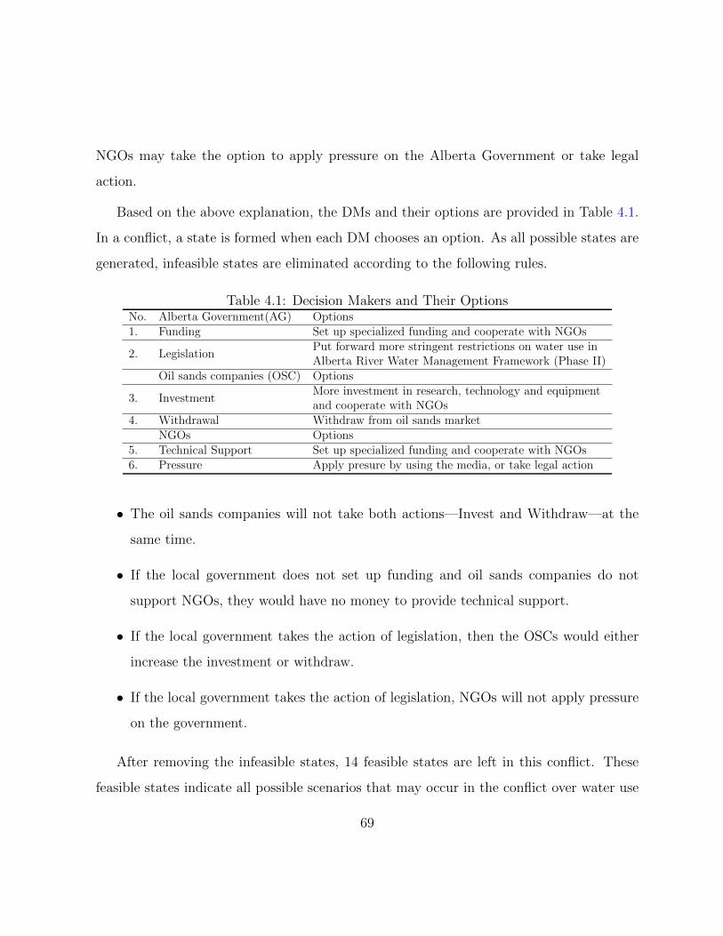
NGOs may take the option to apply pressure on the Alberta Government or take legal

action.

Based on the above explanation, the DMs and their options are provided in Table 4.1.

In a conflict, a state is formed when each DM chooses an option. As all possible states are

generated, infeasible states are eliminated according to the following rules.

Table 4.1: Decision Makers and Their OptionsNo. Alberta Government(AG) Options1. Funding Set up specialized funding and cooperate with NGOs

2. LegislationPut forward more stringent restrictions on water use inAlberta River Water Management Framework (Phase II)

Oil sands companies (OSC) Options

3. InvestmentMore investment in research, technology and equipmentand cooperate with NGOs

4. Withdrawal Withdraw from oil sands marketNGOs Options

5. Technical Support Set up specialized funding and cooperate with NGOs6. Pressure Apply presure by using the media, or take legal action

• The oil sands companies will not take both actions—Invest and Withdraw—at the

same time.

• If the local government does not set up funding and oil sands companies do not

support NGOs, they would have no money to provide technical support.

• If the local government takes the action of legislation, then the OSCs would either

increase the investment or withdraw.

• If the local government takes the action of legislation, NGOs will not apply pressure

on the government.

After removing the infeasible states, 14 feasible states are left in this conflict. These

feasible states indicate all possible scenarios that may occur in the conflict over water use

69

Table 4.2: Decision Makers, Options and Feasible States

AG1. Funding N N N Y N Y N2. Legislation N N Y N N N Y

OSCs3. Investment N Y Y N Y Y Y4. Withdrawal N N N N N N N

NGOs5. Technical Support N N N Y Y Y Y6. Pressure N N N N N N N

Feasible States s1 s2 s3 s4 s5 s6 s7

AG1. Funding Y N N Y N Y –2. Legislation Y N N N N N –

OSCs3. Investment Y N Y N Y Y –4. Withdrawal N N N N N N Y

NGOs5. Technical Support Y N N Y Y Y –6. Pressure N Y Y Y Y Y –

Feasible States s8 s9 s10 s11 s12 s13 s14

and oil sands development in the Athabasca River Basin. They are shown in Table 4.2. In

this table, “Y” indicates that the option is chosen by a DM and “N” means not selected.

A dash, given by “-”, means either a “Y” or “N”. A state is formed when each DM chooses

a strategy. For example, state s14 is created when oil sands companies decide to withdraw

from the market as indicated by the “Y” opposite option 4. The other available option

selections will not affect the conflict as indicated by dashes opposite these options, where

a dash means “Y” or “N”.

At the following stage of modelling using GMCR II, the option prioritizing is used to

estimate the preferences of DMs. In the method, states are ranked according to lexico-

graphic statements (Kilgour and Eden, 2010). The logical preference statements for each

DM are described and explained in Tables 4.3, 4.4 and 4.5. Note that the options of DMs:

Funding, Legislation, Investment, Withdraw, Technical Support, and Apply Pressure are

represented by numbers 1, 2, 3, 4, 5, and 6. Preference statements are given from most

important at the top to least important at the bottom.

70

Table 4.3: Preference Ordering Principals for the Alberta Government

Ordering statements Explanation

-4AG would give most priority to the state where:

OSCs do not withdraw.

-6AG would then give priority to the state where:

NGOs do not take the action of applying pressure

1 IF 6

AG would then give priority to the state where:

If NGOs take the action of applying pressure,

AG prefers providing extra funding.

-2AG would then give priority to the state where:

AG will not take the action of legislation.

1 IF 3AG would then give priority to the state where:

AG would like to provide funding

when OSCs make more investment.

-1AG would then give priority to the state where:

AG do not provide fund.

3AG would then give priority to the state where:

OSCs pay more on research and technology.

5AG would then give priority to the state where:

NGOs provide technical support.

71

Table 4.4: Preference Ordering Principals for Oil Sands CompaniesOrdering statements Explanation

-4OSCs would give most priority to the state where:OSCs do not withdraw.

-2OSCs would then give priority to the state where:AG do not take the action of legislation.

-6OSCs would then give priority to the state where:If NGOs do not take the action of applying pressure.

-3OSCs would then give priority to the state where:OSCs do not make investment.

1OSCs would then give priority to the state where:AG provide extra funding

5OSCs would then give priority to the state where:NGOs provide technical support.

Table 4.5: Preference Ordering Principals for NGOsOrdering statements Explanation

2NGOs would give most priority to the state where:AG take the action of legislation.

6 IF -2NGOs would then give priority to the state where:NGOs take the action of AAPif AG do not set up more stringent restrictions

-6NGOs would then give priority to the state where:If NGOs do not take the action of applying pressure.

3NGOs would then give priority to the state where:OSCs make more investment.

1NGOs would then give priority to the state where:AG provide extra funding.

5NGOs would then give priority to the state where:provide technical support

72

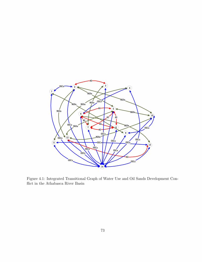
1

14

13

12

11

10

9

87

6

5

43

2

NGOs

OSCs

OSCs

AG

NGOs

NGOs

NGOs

NGOs

NGOs

NGOs

OSCs

AG

AG

OSCs

OSCs

OSCs

OSCs

AG

AG

AG

AG

AG

NGOsNGOs

OSCs

OSCs

OSCs

OSCsOSCs

OSCs

OSCs

NGOs

OSCs

OSCs

Figure 4.1: Integrated Transitional Graph of Water Use and Oil Sands Development Con-flict in the Athabasca River Basin

73

The directed graph for the conflict of water use and oil sands development in the

Athabasca River Basin is shown in Figure 4.1. In the directed graph, the vertices represent

the 14 feasible states, and the arcs labelled by different DMs indicating unilateral moves

of corresponding DMs.

4.5.3 Stability Analysis

Since the preferences of DMs have been determined by option prioritization, and DMs’

unilateral moves are identified as shown in Figure 4.1. In this subsection, a stability

analysis is carried out using GMCR II based on four stability definitions: Nash stability

(R), general metarationality (GMR), symmetric metarationality (SMR), and sequential

stability (SEQ), and the results are shown in Table 4.6. In the conflict, seven states are

calculated as equilibria for all DMs, and these stable states are marked by a√

under the

corresponding stability definitions. The stable states represent the situations that may

happen in the real world. Three representative Nash stable and sequentially stable states

are discussed below:

In state s11, the Alberta Government sets up specialized funding and cooperates with

NGOs in researching the technology to increase efficiency of water use, such recycling water

from tailing ponds. In this situation, NGOs would still apply pressure on the government

and oil sands companies, because upgrading technologies may take a long time to develop

and the public wishes to see a well developed industry without sacrificing the environment.

In state s3, the Alberta Government takes the action of legislation, and the oil sands

companies invest in research, technology and equipment. In this situation, when more oil

sands companies access the market, the conflict over water use and oil sands development

may become more severe. Then the Alberta Government would create tighter legislation, to

74

Table 4.6: Stability Results for the conflict of water use and oil sands development

States s3 s7 s8 s9 s11 s12 s14

AGFunding N N Y N Y N –Legislation Y Y Y N N N –

OSCsInvestment Y Y Y N N Y NWithdrawal N N N N N N Y

NGOsTechnical Support N Y Y N Y Y –Pressure N N N Y Y Y –

R√ √ √

GMR√ √ √ √ √ √ √

SMR√ √ √ √ √ √ √

SEQ√ √ √ √ √

assure that the industry is well monitored. When the quantity of fresh water use is strictly

regulated, there will be fierce competition among oil sands companies in this market. The

companies that effectively use limited quantity of fresh water will survive better in the

future.

In state s8, the Alberta Government will set up specialized funding and cooperates with

NGOs after putting forward more stringent restrictions on water use within the Alberta

River Water Management Framework (Phase II), and NGOs would like to offer technical

support. In addition, oil sands companies would also make extra investment in research,

technology and equipment because of the pressure caused by the competition in the market.

In this situation, The Alberta Government would like to see fierce competition among oil

sands companies which should lead to highly developed technologies, but the government

could not accept that most of the oil sands companies withdraw from the market when

companies cannot afford the cost of research and development. Hence, both the Alberta

Government and oil sands companies will offer funds to accelerate the development of the

75

oil sands industry and reduce environmental effects. This equilibrium indicates a trend:

how the oil sands industry develops from a shorter to longer sighted perspective.

4.6 Conclusions

In this chapter, four main components (DMs, feasible states, possible movements controlled

by each DM, and DM’s preferences) are presented and explained in detail. When a conflict

has two DMs, the concepts of unilateral moves and unilateral improvements for a DM are

provided to identify reachable and preferred states from the initial state in one step by

the DM. These concepts are then extended to deal with a conflict when multiple DM are

involved in a conflict. After that, four basic stability definitions (Nash stability, general

metarationality, symmetric metarationality, and sequential stability) are given along with

their interpretations to carry out stability analysis in a strategic conflict with two or more

DMs.

A conflict over water use and oil sands development in the Athabasca River Basin is

proposed, and a stability analysis is carried out based on GMCR. In order to balance

industrial development and environmental protection, the conflict among the Alberta gov-

ernment, oil sands companies, and non-governmental organizations is investigated. Seven

states of the conflict are determined as equilibria according to the aforementioned four

stability definitions, and interpretations for these equilibria are provided.

76

Chapter 5

Grey-based Preference in a Graph

Model for Conflict Resolution with

Two Decision Makers

The research contained in this chapter constitutes a significant expansion of classical Graph

Model for Conflict Resolution (GMCR). The new methodology, using grey numbers to

express uncertain preferences of DMs, formally puts forward grey preferences, and defines

grey-based stability definitions within the GMCR structure, thereby extending the graph

model methodology. Corresponding grey-based equilibria can then be identified, indicating

more realistic resolutions for conflicts in the face of uncertainty.

In the literature, many studies have been conducted to address group decision making

with uncertain preference information. For example, Han et al. (2013) concentrated on

modelling grey conflict analysis based on grey input data, while Ben-Haim and Hipel

(2002) used the information-gap model to estimate uncertainty of preference for DMs.

77

Figure 5.1: Main Contributions within the Framework of Conflict Analysis

78

Li et al. (2004) put forward a new preference relation—“prefer to”, “indifferent to”, and

“unknown”—in modelling preference uncertainty in the graph model. Bashar et al. (2012)

and Hipel et al. (2011) developed a fuzzy preference methodology to model and analyse

conflicts under fuzzy preference uncertainty.

The main contributions of this approach within the framework of conflict analysis are

shown in Figure 5.1, which is modified from Fang et al. (1993), and Fraser and Hipel

(1984). Modelling a real-world conflict consists of identifying the DMs, their options, and

their relative preferences over states. The current research extends the classical GMCR by

mathematically defining grey preferences, grey stabilities, and grey equilibria. Moreover,

interpretation and sensitivity analyses are carried out using a sustainable development

conflict. The results can assist the DMs to make informed strategic choices.

5.1 Grey Preference Structure in the Graph Model

In the following subsections, the fundamental concepts of grey preference degree, grey

relative certainty of preference, anticipated preference, grey satisficing threshold, and grey

unilateral improvements are defined. These definitions are analogous, but different, to

the corresponding definitions for fuzzy preferences in GMCR (Bashar et al., 2012), (Hipel

et al., 2011). Based on these definitions, the concept of grey preference is incorporated into

the graph model methodology, and four basic grey stability definitions in a conflict with

two DMs are described.

79

5.1.1 Grey Preference Degree

When a DM needs to make a choice between two alternatives, sometimes he may easily

make the decision, and strictly prefers one over another. For example, a vegetarian def-

initely prefers vegetables over meat; however, in some situations, it is hard for the DM

to choose. For example, a vegetarian may be not sure whether he will cook tomato or

potato for lunch. Then, uncertain preferences can capture a DM’s intuition on how much

an alternative is preferred to the other. A grey preference expresses uncertain preferences

of DMs in a general way using generalized grey numbers, ranging from 0 to 1 (Kuang

et al., 2013). Depending on the degree of uncertainty, a grey preference structure allows

DMs to represent their preferences in different forms flexibly. For example, a DM can

show his preference of one alternative over another as a value, 0.6, an interval, [0.2, 0.4],

or a combination of intervals, [0.3, 0.4], [0.5, 0.6]. The elements in these grey numbers

represent the DM’s possible preference degree for one state over another. Grey preferences

constitute an extension of GMCR preference structures.

Definition 5.1 Grey Preference Degree: Let D[0, 1]⊗ represent the set of all grey

numbers within the interval [0, 1]. A grey preference is an m×m matrix of grey numbers,

⊗P = (⊗pij)m×m, denoted as

⊗ p(si, sj) = ⊗pij ∈ D[0, 1]⊗, (5.1)

the GPD of state si over sj satisfies ⊗pii = 0.5 for i = 1, 2, . . . ,m, and if ⊗pij ∈L⋃l=1

[p−ijl, pij

l], then ⊗pji ∈L⋃l=1

[1− pjil, 1− p−jil] for i, j = 1, 2, . . . ,m.

The grey-based preference degrees provided by Definition 5.1 can be interpreted as

follows:

80

(1) ⊗p(si, sj) = 0 indicates state sj is strictly preferred to si.

(2) ⊗p(si, sj) ∈ D[0, 0.5]⊗ and ⊗p(si, sj) 6= 0, 0.5 indicates state si is less likely to be

preferred to sj.

(3) ⊗p(si, sj) = 0.5 means state si is equally likely to be preferred to sj.

(4) ⊗p(si, sj) ∈ D[0.5, 1]⊗ and ⊗p(si, sj) 6= 0.5, 1 indicates state si is more likely to be

preferred to sj.

(5) ⊗p(si, sj) = 1 indicates state si is strictly preferred to sj.

Then, the grey preferences of DM k over all possible pairs of states in S can be rep-

resented by a grey preference matrix (⊗P k)m×m, generated through pairwise comparison

among all possible pairwise combinations of states, and written as follows:

⊗ P k =

⊗pk11 ⊗pk12 ... ⊗pk1m⊗pk21 ⊗pk22 ... ⊗pk2m... ... ... ...

⊗pkm1 ⊗pkm2 ... ⊗pkmm

(5.2)

Note that an entry in ⊗P k indicates DM k’s preference degree for the row state over the

column state.

Three examples are provided so as to further interpret grey preference structure. They

are introduced as follows:

Example 5.1 A brownfield property is for sale, and the government (G) has two options:

offer financial and policy incentives (O) or not (N). From its own perspective, the gov-

ernment would prefer the option of N. However, successful redevelopment of the brownfield

can increase tax revenue and employment opportunities, and remove the potential threat of

81

pollution. The preference for N over O is ⊗PGNO = 0.8. This uncertain preference means

the government does not definitely prefer N or O, but it is more likely to prefer N . Then,

the preference matrix can be written as:

⊗PG =

O N

O 0.5 0.2

N 0.8 0.5

Example 5.2 After a period of time, the property has not been sold, and citizens ask for

environmental remediation. Considering the potential income after the property redevelop-

ment and the possible social impacts, the government’s preference over these two states has

changed, and its preferences move from (N) towards O. However, it is hard to estimate the

magnitude of its preferences change. Therefore, the uncertain preferences are represented

using interval values. Compared with the preferences in Example 5.1, interval preferences

mean that N is preferred over O for the government in general, but the degree of preference

is not sure. The preference matrix for the government becomes:

⊗PG =

O N

O 0.5 [0.2, 0.4]

N [0.6, 0.8] 0.5

Example 5.3 Later, it is clear that no buyer wants to purchase this property because of

the potential risk of pollution, which may lead to endless liability regarding the cleanup of

hazardous materials. An overall assessment of onsite contamination is undertaken. The

government is eager to facilitate the transaction as soon as possible, and it is reluctant to

wait for the assessment results. In this situation, considering the degree of pollution, its

preferences of N over O are split into two parts. If the property is highly contaminated the

82

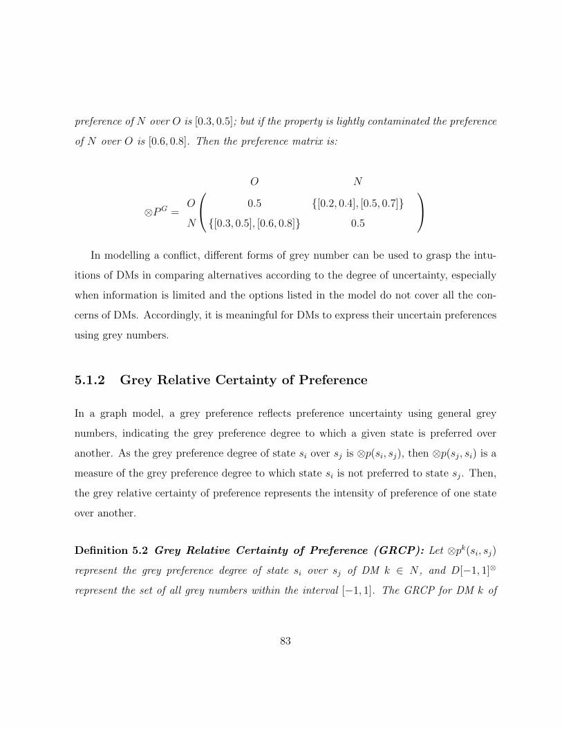
preference of N over O is [0.3, 0.5]; but if the property is lightly contaminated the preference

of N over O is [0.6, 0.8]. Then the preference matrix is:

⊗PG =

O N

O 0.5 [0.2, 0.4], [0.5, 0.7]

N [0.3, 0.5], [0.6, 0.8] 0.5

In modelling a conflict, different forms of grey number can be used to grasp the intu-

itions of DMs in comparing alternatives according to the degree of uncertainty, especially

when information is limited and the options listed in the model do not cover all the con-

cerns of DMs. Accordingly, it is meaningful for DMs to express their uncertain preferences

using grey numbers.

5.1.2 Grey Relative Certainty of Preference

In a graph model, a grey preference reflects preference uncertainty using general grey

numbers, indicating the grey preference degree to which a given state is preferred over

another. As the grey preference degree of state si over sj is ⊗p(si, sj), then ⊗p(sj, si) is a

measure of the grey preference degree to which state si is not preferred to state sj. Then,

the grey relative certainty of preference represents the intensity of preference of one state

over another.

Definition 5.2 Grey Relative Certainty of Preference (GRCP): Let ⊗pk(si, sj)

represent the grey preference degree of state si over sj of DM k ∈ N , and D[−1, 1]⊗

represent the set of all grey numbers within the interval [−1, 1]. The GRCP for DM k of

83

state si relative to sj is

⊗ rk(si, sj) = ⊗pk(si, sj)−⊗pk(sj, si) (5.3)

In (5.3), ⊗rk(si, sj) ∈D[−1, 1]⊗. To assist in further interpretation, the following properties

are provided. For DM k,

(1) ⊗rk(si, sj) = −1 indicates state sj is strictly preferred to si. A simplified notation

for ⊗rk(si, sj) is ⊗rkij. Then, a grey relative certainty of preference for DM k over S is

represented by a matrix (⊗rkij)m×m.

(2) ⊗rk(si, sj) ∈ D[−1, 0]⊗ and ⊗rk(si, sj) 6= −1, 0 indicates state si is less likely to be

preferred to sj.

(3) ⊗rk(si, sj) = 0 indicates state si is equally likely to be preferred to sj.

(4) ⊗rk(si, sj) ∈ D[0, 1]⊗ and ⊗rk(si, sj) 6= 0, 1 indicates state si is more likely to be

preferred to sj.

(5) ⊗rk(si, sj) = 1 indicates state si is strictly preferred to sj.

⊗ rk =

⊗rk11 ⊗rk12 ... ⊗rk1m⊗rk21 ⊗rk22 ... ⊗r2m

... ... ... ...

⊗rkm1 ⊗rkm2 ... ⊗rkmm

(5.4)

Example 5.4 Based on the preferences of Example 5.2, the grey relative certainty of pref-

erence of the government is:

84

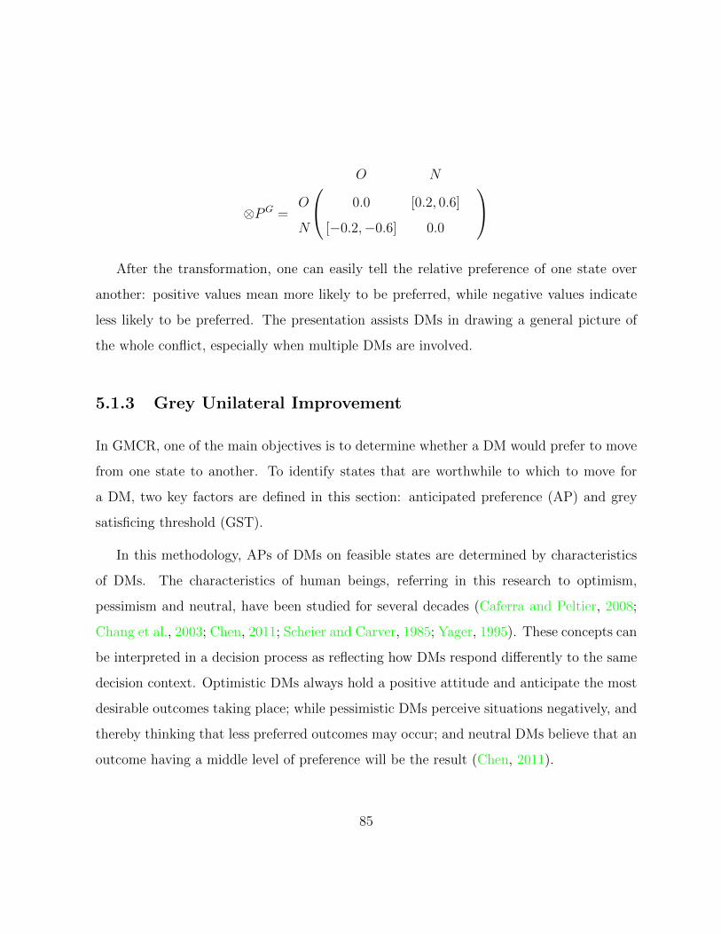
⊗PG =

O N

O 0.0 [0.2, 0.6]

N [−0.2,−0.6] 0.0

After the transformation, one can easily tell the relative preference of one state over

another: positive values mean more likely to be preferred, while negative values indicate

less likely to be preferred. The presentation assists DMs in drawing a general picture of

the whole conflict, especially when multiple DMs are involved.

5.1.3 Grey Unilateral Improvement

In GMCR, one of the main objectives is to determine whether a DM would prefer to move

from one state to another. To identify states that are worthwhile to which to move for

a DM, two key factors are defined in this section: anticipated preference (AP) and grey

satisficing threshold (GST).

In this methodology, APs of DMs on feasible states are determined by characteristics

of DMs. The characteristics of human beings, referring in this research to optimism,

pessimism and neutral, have been studied for several decades (Caferra and Peltier, 2008;

Chang et al., 2003; Chen, 2011; Scheier and Carver, 1985; Yager, 1995). These concepts can

be interpreted in a decision process as reflecting how DMs respond differently to the same

decision context. Optimistic DMs always hold a positive attitude and anticipate the most

desirable outcomes taking place; while pessimistic DMs perceive situations negatively, and

thereby thinking that less preferred outcomes may occur; and neutral DMs believe that an

outcome having a middle level of preference will be the result (Chen, 2011).

85

Note that GRCP, introduced in Definition 5.2, is represented in the form of a general

grey number. Then, AP is employed to estimate the preference of a DM expressed by

GRCP, based on three types of characteristics of DMs: optimistic, pessimistic and neutral.

Definition 5.3 Anticipated Preference (AP): For k ∈ N , si, sj ∈ S, let ⊗rk(si, sj) ∈n⋃l=1

[x−l, xl] denote the grey relative certainty of preference of si relative to sj for DM k, and

let r−ijk and rij

k represent the lower bound and the upper bound of ⊗rk(si, sj) ∈n⋃l=1

[x−l, xl],

respectively. Then, the DM k’s AP for si over sj, denoted as AP k(si, sj), is:

• If DM k is pessimistic, then

AP k(si, sj) = r−ijk (5.5)

• If DM k is optimistic, then

AP k(si, sj) = rijk (5.6)

• If DM k is neutral, then

AP k(si, sj) =

1n

n∑l=1

x−l, if x−l = xl for all l = 1, 2, . . . , n

n∑l=1

(xl−xl)(xl+xl

2)

n∑i=1

(xl−xl), otherwise

(5.7)

To assist in understanding these concepts, note that:

• Uncertain preferences over feasible states are represented with general grey numbers,

which may consist of a set of intervals. A discrete value is the special case, in which

the upper and lower bounds are the same.

86

• A pessimistic DM, holding a negative attitude, construes AP as the lower bound of

GRCP.

• An optimistic DM, having a positive attitude, interprets AP as the upper bound of

GRCP.

• The AP of a neutral DM is the centre of his GRCP. It can be further interpreted in

two forms: the average of the values when they are all discrete; the calculation of AP

depends on the mid-point and the length of each interval when intervals are present.

Discrete values are not used in this calculation, since they are intervals having no

width.

Definition 5.4 Grey Satisficing Threshold (GST): For k ∈ N and s, si ∈ S, let

AP k(si, s) denote AP of DM k for state si over s. Let γk be a real number such that

AP k(si, s) > γk implies DM k would prefer to move from state s to si. Then γk is called

the GST of DM k.

Note that 0 < γk 6 1. The GST of a DM is the degree of confidence that characterizes

whether the DM finds a move worthwhile. Note that DMs may have different GSTs. In a

grey-based preference structure, the decision to move or not is made by analysing the AP

of the target state over the initial state. A DM will move from the initial state only to a

state for which the AP is greater or equal to the DM’s GST. For example, an aggressive

DM may have a GST of 0.3, but a conservative DM may have a GST of 0.7. The latter

DM would move to a state only when its AP over the initial state is not less than 0.7.

Since GRCP, AP, and GST have been formally defined, a DM’s grey unilateral im-

provement is formally defined below:

87

Definition 5.5 Grey Unilateral Improvement (GUI) for a DM: For k ∈ N and

s ∈ S, let γk be the grey satisficing threshold for DM k. Recall that Rk(s) denotes the set

of states reachable from the state s for DM k. A state si ∈ Rk(s) is called a GUI from s

for DM k with respect to γk, if and only if AP k(si, s) > γk.

A GUI is a preferred state that is reachable by a DM from the initial state. Specifically, a

GUI is a reachable state for which AP over the initial state is greater than or equal to the

GST of the DM.

Definition 5.6 Grey Unilateral Improvement (GUI) list for a DM: For s ∈ S

and k ∈ N , let Rk(s) denote the set of states reachable from the state s by DM k, and γk be

the grey satisficing threshold for DM k. The GUI list, denoted ⊗R+k,γk

(s), is the collection

of all GUIs from s for DM k with respect to γk, represented mathematically as

⊗R+k,γk

(s) = si ∈ Rk(s) : AP k(si, s) > γk (5.8)

5.2 Grey Stabilities in a Conflict with Two Decision

Makers

In GMCR, stability analysis aims to identify stable states for DMs participating in a

strategic interaction. The initial state, stable or not, is called the status quo. The DM

who has the right to move is called the focal DM. In a graph model with grey preferences,

a GUI for a DM is a state to which the DM wishes to move. However, sanctions may be

imposed by the other DM, and the focal DM may end up at less preferred states compared

with the initial state. In this case, the initial state is stable.

88

In this section, the four basic grey-based stabilities in a strategic conflict are defined

for a graph model with two DMs. Specifically, grey Nash stability (GR), grey general

metarationality (GGMR), grey symmetric metarationality (GSMR), and grey sequential

stability (GSEQ) are introduced. Note that these definitions depend on the grey preference

structure that was described in Section 5.1.

Recall that S = s1, s2,. . . , sm, m > 1 denotes the set of feasible states, and N = p, q

represents the set of two DMs. Then, GSTs for each DM, the APs for si over sj, and GUIs

from s of each DM are respectively denoted as γp and γq, APp(si, sj) and AP q(si, sj), and

⊗R+p,γp(s) and ⊗R+

q,γq(s). The formal definitions of the four grey stabilities are given below.

Definition 5.7 Grey Nash Stable (GR): A state s ∈ S is GR for DM p, denoted by

s ∈ SGRp , if and only if ⊗R+p,γp(s) = ∅.

In GR stability, the focal DM will definitely move to a more preferred state based on his

AP and GST without considering possible subsequent countermoves by the other DM. In

other words, for the focal DM, no state reachable from the initial state is more preferred,

based on his satisficing criterion. Specifically, a state s ∈ S is GR stable for DM p if and

only if DM p has no GUI from s.

Theorem 5.7.1 Suppose that for every DM k, ⊗rk(si, sj), the grey relative preference of

DM k for si over sj, equals either 1 or -1, for all states si, sj ∈ S. Then a state s ∈ S is

grey Nash stable iff s is Nash stable in classical GMCR.

Proof: Let N = p, q be the set of DMs, and let γp denote the GST of p. Let

⊗R+p,γp(s) = si ∈ Rk(s) : AP p(si, s) > γp represent the grey unilateral improvement

list from state s for DM p. If ⊗rp(si, sj) ∈ 1,−1, then AP p(si, sj) = r−ijp = rij

p =

89

⊗rp(si, sj) ∈ 1,−1. Therefore, ⊗rp(si, s) ≥ γp ≡ ⊗rp(si, s) = 1. Based on the grey

preference relation, ⊗rp(si, s) = 1 indicates si p s. Hence, if ⊗rp(si, sj) ∈ 1,−1,

⊗R+p,γp(s) = si ∈ Rp(s) : AP p(si, s) > γp = ∅ if and only if ⊗R+

p (s) = si ∈ Rp(s) : si ps = ∅.

Remark: Theorem 5.7.1 extends to the following three grey stability definitions.

Therefore, stability definitions of classical GMCR are special cases of grey-based GMCR.

Definition 5.8 Grey General Metarational (GGMR): A state s ∈ S is GGMR for

DM p, denoted by s ∈ SGGMRp , if and only if for every s1 ∈ ⊗R+

p,γp(s) there exists at least

one s2 ∈ Rq(s1) such that AP p(s2, s) < γp.

In GGMR stability, the focal DM needs to consider not only his possible GUIs but also

subsequent unilateral movements of the other DM. Specifically, a state s is GGMR for DM

p if and only if moving to any GUI from s by DM p can be sanctioned by a subsequent

unilateral movement of DM q. In other words, if p chooses to move from s to a GUI,

s1, DM q has at least one unilateral movement from state s1 to a state s2, which is less

preferred by DM p compared with s, based on his satisficing criterion.

Definition 5.9 Grey Symmetric Metarational (GSMR): A state s ∈ S is GSMR

for DM p, denoted by s ∈ SGSMRp , if and only if for every s1 ∈ ⊗R+

p,γp(s) there exists at

least one s2 ∈ Rq(s1) such that AP p(s2, s) < γp, and AP p(s3, s) < γp for all s3 ∈ Rp(s2).

In GSMR stability, the focal DM needs to consider not only his possible GUIs but also

subsequent unilateral movements of the other DM, as well as the focal DM’s possible

counter-reactions. Specifically, a state s is GSMR for DM p if and only if moving to any

GUI from s by DM p can be sanctioned by a subsequent unilateral movement by DM q,

90

and DM p cannot escape this sanction by another unilateral movement. In other words, if

DM p chooses to move to a GUI s1 from s, DM q has a subsequent unilateral movement

from state s1 to s2, which is not advantageous for DM p to move from s, and so is any

unilateral movement of DM p from s2, based on his satisficing criterion.

Theorem 5.9.1 If state s ∈ S is grey symmetric metarationally stable for DM p, then s

is grey general metarational stable for DM p.

Proof: For N = p, q, let Rp(s) represent the reachable list from state s for DM p, and

let ⊗R+p,γp(s) = si ∈ Rp(s) : AP p(si, s) > γp represent the grey unilateral improvement

list from state s for DM p. If s is grey symmetric metarationally stable for DM p, then for

any s1 ∈ ⊗R+p,γp(s) there exists at least one s2 ∈ Rq(s1) such that AP p(s2, s) < γp. Hence,

s is grey general metarational for DM p.

Remark: GSMR adds a restriction to GGMR. Therefore, if s is GSMR, it must also be

GGMR. GGMR is used to define a noncooperative situation, where the opponent may take

actions to sanction the focal DM’s improvement without considering his own preferences.

GSMR is applicable for DMs having strategic foresight. The focal DM needs to consider

not only whether his improvement will be sanctioned by the opponent’s countermoves, but

also whether he can escape from this sanction.

Definition 5.10 Grey Sequentially Stable (GSEQ): A state s ∈ S is GSEQ for DM

p, denoted by s ∈ SGSEQp , if and only if for every s1 ∈ ⊗R+p,γp(s) there exists at least one

s2 ∈ R+q,γq(s1) such that AP p(s2, s) < γp.

In GSEQ stability, the focal DM needs to consider not only his possible GUIs but also

subsequent GUIs of the other DM. Specifically, a state s is GSEQ stable for DM p, if and

91

only if moving to any GUI from s by DM p can be sanctioned by a subsequent GUI of

DM q. Stated differently, if DM p moves to a GUI s1 from state s, DM q has at least one

GUI from state s1 to s2, which is less preferred for DM p compared with s, based on his

satisficing criterion.

Theorem 5.10.1 If state s ∈ S is grey sequentially stable for DM k, then s is grey general

metarational stable for DM k.

Proof: For N = p, q, let Rp(s) represent the reachable list from state s for DM p, and

let ⊗R+p,γp(s) = si ∈ Rp(s) : AP p(si, s) > γp stand for the grey unilateral improvement

list from state s for DM p. If s is grey sequentially stable for DM p, then for every

s1 ∈ ⊗R+p,γp(s) there exists at least one s2 ∈ R+

q,γq(s1) such that AP p(s2, s) < γp. Note

that ⊗R+p,γp(s) ⊆ ⊗Rp,γp(s), that is, for every s1 ∈ ⊗R+

p,γp(s) there exists at least one

s2 ∈ Rq(s1) such that AP p(s2, s) < γp. Hence, s is grey general metarational stable for

DM p.

Remark: In general, because every unilateral improvement is also an unilateral move-

ment, GSEQ implies GGMR. Hence, if s is GSEQ, it will also be GGMR. Compared with

GGMR, GSEQ is suitable when the opponent only considers sanctioning the focal DM’s

improvement when he can benefit from the counter move.

Theorem 5.10.2 If a state s ∈ S is grey Nash stable for DM k, then s is also grey general

metarationally stable, grey symmetric metarationally stable, and grey sequentially stable for

DM k.

Proof: For N = p, q, let Rp(s) represent the reachable list from state s for DM p, and

let ⊗R+p,γp(s) = si ∈ Rp(s) : AP p(si, s) > γp stand for the grey unilateral improvement

92

list from state s for DM p. If s is grey Nash stable for DM p, then ⊗R+p,γp(s) = ∅. Hence,

Definitions 5.8, 5.9, and 5.10 are satisfied.

Remark: If a state s is GR for DM p, then the DM does not have any GUI from s to

which to move. This also means that no GUI from s by DM p can be sanctioned by the

opponent using any unilateral movement or GUI. Finding the relations among the stability

definitions is helpful for interpreting a conflict in the process of stability analysis.

Definition 5.11 A state s ∈ S is called a grey equilibrium under a specific grey stability

definition if and only if the state is grey stable for each DM under that grey stability

definition.

5.3 Case Study: Sustainable Development Conflict

under Uncertainty

5.3.1 Background

The sustainable development conflict is a hypothetical generic conflict originally proposed

by Hipel (2002). In this section, Grey-based GMCR, is applied to this conflict to for-

mally handle preference uncertainty experienced by one of the two DMs. This application

illustrates how the grey-based solution concepts can be used to analyse a conflict with

two DMs having uncertain preferences. The fundamental components for the conflict are

summarized as follows (Hipel, 2002):

• DMs: The model consists of two groups of DMs—Environmental agencies (ENV)

and Developers (DEV).

93

• Options: ENV, aiming to meet human needs while protecting the environment from

possible harm, can be proactive or reactive in monitoring the activities of DEV. DEV

can choose sustainable development or unsustainable development. In summary, the

options for ENV are to be (i) proactive or (ii) reactive, while the options for DEV

are to practice (i) sustainable development or (ii) unsustainable development.

• Feasible States: Four feasible states are identified and listed in Table 5.1, in which

“Y” means that the option is chosen and “N” means not selected. There are 4 states

in this conflict, for which a state is formed when each DM chooses a strategy. For

example, state s1 is created when ENV is proactive in monitoring the activities of

DEV, while DEV selects sustainable development.

Table 5.1: Feasible States for the Sustainable Development Conflict

ENVProactive Y Y N N

DEVSustainable Y N Y N

States Number s1 s2 s3 s4

The directed graph in Figure 5.2 shows available transitions by ENV and DEV in

a graph model. In this graph, the nodes represent the 4 feasible states for ENV and

DEV, while the directed arcs, labelled by the DMs, represent their respective unilateral

movements.

As mentioned above, in the original sustainable development conflict, uncertain pref-

erences of DMs were not taken into account. However, the DMs involved in the conflict

94

S1

S4S3

S2DEV

ENVENV

DEV

Figure 5.2: The Graph Model of Movement for the Sustainable Development Conflict

may be uncertain about preferences over the feasible states. Li et al. (2004) mentioned

that preferences of DEV may be uncertain because they may be influenced by enforcement

measures of ENV, and some members of DEV may feel more responsible for environmental

protection.

5.3.2 Graph Model with Uncertainty

This research uses grey numbers to represent preferences of the DMs. Based on research

for the sustainable development conflict conducted by Hipel (2002), Li et al. (2004), and

Bashar et al. (2012), it is reasonable to assume that preferences of ENV over feasible states

are all certain, and DEV has preference uncertainty between some states. Moreover, it is

assumed that ENV is pessimistic and DEV is neutral (Hipel, 2002; Li et al., 2004). Then,

through pairwise comparisons over the four feasible states, grey preference matrices are

generated for ENV and DEV as listed in Table 5.2.

Note that for PENV , the preference degrees are a single discrete values consisting of 1 or

0, representing certain preferences. In PDEV , ⊗p12 ∈ [0.1, 0.3] represents DEV’s preference

of sustainable development over unsustainable development when ENV is proactive. This

95

Table 5.2: Grey Preference Matrices of ENV and DEV

DMs Grey preference matricess1 s2 s3 s4

PENV

s1 0.5 1.0 1.0 1.0s2 0.0 0.5 0.0 1.0s3 0.0 1.0 0.5 1.0s4 0.0 0.0 0.0 0.5

PDEV

s1 0.5 [0.1, 0.3] 0.0 0.0s2 [0.7,0.9] 0.5 [0.3,0.4],[0.55,0.75] 0.0s3 1.0 [0.25,0.45],[0.6,0.7] 0.5 0.0s4 1.0 1.0 1.0 0.5

uncertainty is because some members of DEV may feel more responsible for environmen-

tal protection (Hipel and Walker, 2011). The expression ⊗p23 ∈ [0.25, 0.45], [0.6, 0.7]

indicates DEV’s preference of sustainable development when ENV is reactive over unsus-

tainable development when ENV is proactive. For DEV, this uncertainty is influenced by

two main factors. One is that the level of enforcement measures is unknown, and hence

preferences are split into two parts. In this situation, the preference of DEV does not

change consistently. Specifically, if ENV adopts a higher level of enforcement measures,

unsustainable development may be punished heavily. Thus, s2 is less preferred than s3 for

DEV. On the contrary, if a lower level of enforcement measures is applied by ENV, possi-

ble countermeasures may be taken by DEV to achieve more profit through unsustainable

development. Then, s2 is more preferred than s3 for DEV. The other factor is that some

members of DEV may not agree with others. For example, some members may prefer

sustainable development even when ENV employs a lower level of enforcement measures.

This is the reason why each split part is expressed with an interval.

96

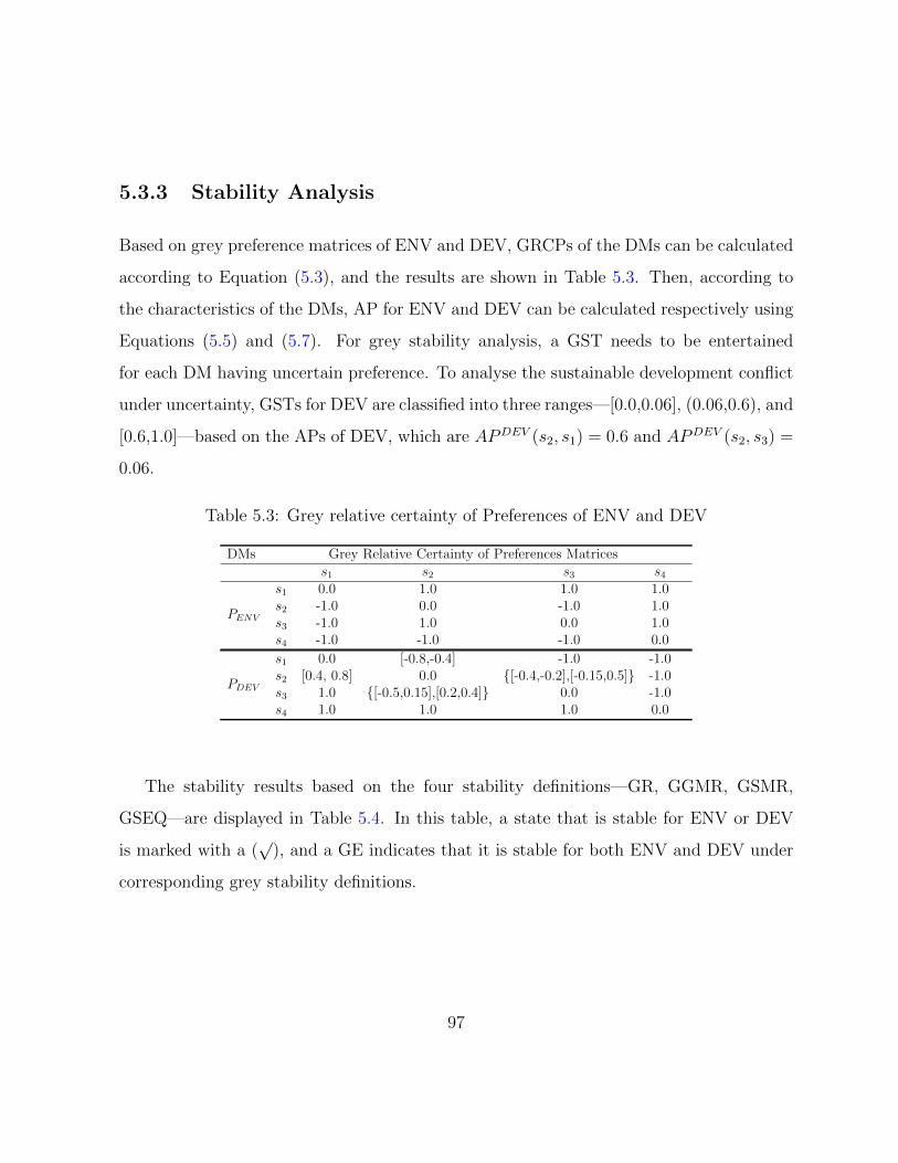
5.3.3 Stability Analysis

Based on grey preference matrices of ENV and DEV, GRCPs of the DMs can be calculated

according to Equation (5.3), and the results are shown in Table 5.3. Then, according to

the characteristics of the DMs, AP for ENV and DEV can be calculated respectively using

Equations (5.5) and (5.7). For grey stability analysis, a GST needs to be entertained

for each DM having uncertain preference. To analyse the sustainable development conflict

under uncertainty, GSTs for DEV are classified into three ranges—[0.0,0.06], (0.06,0.6), and

[0.6,1.0]—based on the APs of DEV, which are APDEV (s2, s1) = 0.6 and APDEV (s2, s3) =

0.06.

Table 5.3: Grey relative certainty of Preferences of ENV and DEV

DMs Grey Relative Certainty of Preferences Matricess1 s2 s3 s4

PENV

s1 0.0 1.0 1.0 1.0s2 -1.0 0.0 -1.0 1.0s3 -1.0 1.0 0.0 1.0s4 -1.0 -1.0 -1.0 0.0

PDEV

s1 0.0 [-0.8,-0.4] -1.0 -1.0s2 [0.4, 0.8] 0.0 [-0.4,-0.2],[-0.15,0.5] -1.0s3 1.0 [-0.5,0.15],[0.2,0.4] 0.0 -1.0s4 1.0 1.0 1.0 0.0

The stability results based on the four stability definitions—GR, GGMR, GSMR,

GSEQ—are displayed in Table 5.4. In this table, a state that is stable for ENV or DEV

is marked with a (√

), and a GE indicates that it is stable for both ENV and DEV under

corresponding grey stability definitions.

97

Table 5.4: Stability Results for the Sustainable Development Conflict under Uncertainty -

with Neutral DEV

GST StatesGR GGMR GSMR GSEQ

ENV DEV GE ENV DEV GE ENV DEV GE ENV DEV GE

s1

√ √ √ √

[0.0,0.06] s2

√ √ √ √ √ √ √ √ √ √ √ √

s3

√ √ √

s4

√ √ √ √

s1

√ √ √ √

(0.06,0.6) s2

√ √ √ √ √ √ √ √ √ √ √ √

s3

√ √ √ √ √ √ √ √ √

s4

√ √ √ √

s1

√ √ √ √ √ √ √ √ √ √ √ √

[0.6,1.0] s2

√ √ √ √ √ √ √ √ √ √ √ √

s3

√ √ √ √ √ √ √ √ √

s4

√ √ √ √

5.3.4 Insights and Sensitivity Analysis

The findings in Table 5.4 provide some insights into the sustainable development conflict

under uncertainty. When the GST ranges from 0 to 0.06, only one state, s2, is stable. In

state s2, ENV is proactive, and DEV prefers unsustainable development. This result is

exactly the same as the stability analysis conducted by Hipel (2002) when DEV definitely

prefers unsustainable states to sustainable development, and uncertainty is not considered.

When the GST takes a value from 0.06 to 0.6, a sustainable development state, s3, and

an unsustainable state, s2, become stable. This result may be caused by the enforcement

measures chosen by ENV, or by the environmentally friendly members of DEV. In this

situation, it may not be worthwhile for DEV to move from a sustainable state to an

98

unsustainable state. When the GST is increased to the range of [0.6,1.0], state s1 becomes

a new grey equilibrium, while s2 and s3 remain equilibria. Potentially, both ENV and DEV

may search for a proper balance between the needs for social-economic development and

environmental protection.

From the above results, a trend can be identified: as the GST increases, the equilibria

change from unsustainable states to sustainable ones. To interpret this trend, notice that,

the uncertain preference of DEV expressed by grey numbers reflects the higher environmen-

tal awareness of DEV members and their sensitivity to the potential enforcement measures

levied by ENV. Based on the grey preference matrix for DEV, the majority of members

of DEV are profit-driven, and put a higher priority on unsustainable development. Recall

that for a GUI, APs must exceed GST. In this case study, the more GST increases, the

more members of DEV practising sustainability need to be considered. In other words,

when the GST is lower, sustainable development is more preferred. On the other hand,

with the increase of the GST, sustainable development will gain more priority. Thus, if

ENV can make more members realize the importance of environmental protection, or em-

ploy a higher level of enforcement measures against unsustainable development, a win-win

relationship between ENV and DEV may be achieved.

In this case study, the characteristic of DEV is assumed to be neutral. To have a

better understanding of grey-based GMCR, extra stability analyses are conducted when

the characteristic of DEV is pessimistic or optimistic, and the results are shown in Tables

5.5 and 5.6, respectively. Based on the lower bound and the upper bound of each grey

number, representing GRCPs of DEV, the GSTs of the DMs are classified into four ranges:

[0.0,0.4], (0.4,0.5], (0.5,0.8], and (0.8,1.0]. It is easy to conclude from the results the least

stable states can be reached when DEV is optimistic, while the most stable states are

available when DEV is pessimistic. These findings are caused by different definitions of

99

AP for DEV. It is clear that if a state is a GUI when DEV is pessimistic, it must also be

a GUI when DEV is neutral or optimistic; and if a state is a GUI when DEV is neutral, it

must also be a GUI when DEV is optimistic. As a consequence, if a state is stable when

DEV is optimistic, it must also be stable when DEV is neutral or pessimistic; and if a state

is stable when DEV is neutral, it must also be stable when DEV is pessimistic.

Table 5.5: Stability Findings for the Sustainable Development Conflict under Uncertainty- with Pessimistic DEV

GST StatesGR GGMR GSMR GSEQ

ENV DEV GE ENV DEV GE ENV DEV GE ENV DEV GEs1

√ √ √ √

[0.0,0.4] s2

√ √ √ √ √ √ √ √ √ √ √ √

s3

√ √ √ √ √ √

s4

√ √ √ √

s1

√ √ √ √ √ √ √ √ √ √ √ √

(0.4,0.5] s2

√ √ √ √ √ √ √ √ √ √ √ √

s3

√ √ √ √ √ √ √ √ √

s4

√ √ √ √

s1

√ √ √ √

(0.5,0.8] s2

√ √ √ √ √ √ √ √ √ √ √ √

s3

√ √ √ √ √ √ √ √ √

s4

√ √ √ √

s1

√ √ √ √ √ √ √ √ √ √ √ √

(0.8,1.0] s2

√ √ √ √ √ √ √ √ √ √ √ √

s3

√ √ √ √ √ √ √ √ √

s4

√ √ √ √

5.4 Conclusions

The proposed methodology of grey-based GMCR forms a solid framework for conflict res-

olution under uncertainty. Grey numbers allow DMs to express their uncertain preferences

based on their particular concerns, and can provide more information for DMs to make

more enlightened decisions.

100

Table 5.6: Stability Results for the Sustainable Development Conflict under Uncertainty -with Optimistic DEV

GST StatesGR GGMR GSMR GSEQ

ENV DEV GE ENV DEV GE ENV DEV GE ENV DEV GEs1

√ √ √ √

[0.0,0.4] s2

√ √ √ √ √ √ √ √ √ √ √ √

s3

√ √ √

s4

√ √ √ √

s1

√ √ √ √

(0.4,0.5] s2

√ √ √ √ √ √ √ √ √ √ √ √

s3

√ √ √

s4

√ √ √ √

s1

√ √ √ √

(0.5,0.8] s2

√ √ √ √ √ √ √ √ √ √ √ √

s3

√ √ √ √ √ √ √ √ √

s4

√ √ √ √

s1

√ √ √ √ √ √ √ √ √ √ √ √

(0.8,1.0] s2

√ √ √ √ √ √ √ √ √ √ √ √

s3

√ √ √ √ √ √ √ √ √

s4

√ √ √ √

In this work, a grey preference structure was introduced, and related definitions (GUI,

GST, and AP) were presented to facilitate DMs to make judgements when they have

uncertain preferences. Then, four solution concepts (GR, GGMR, GSMR, and GSEQ)

were defined and related theorems put forward. It was also demonstrated that stability

definitions of classical GMCR are special cases of grey-based GMCR.

A case study of sustainable development with two DMs was carried out. Through

the comparison with classical GMCR, the grey-based stability analysis results suggested a

trend in how the equilibria change. This trend can be helpful for finding the reality hidden

behind the uncertainty, and can also assist DMs to estimate the potential evolution of the

conflict. In real-world applications, if one can discover where the source of the uncertainty

lies, and determine stability analysis results generated by the grey based graph model, the

influence of uncertainty on the conflict may be better understood. Therefore, DMs can

put appropriate countermeasures in place to influence the evolution of the conflict.

101

Chapter 6

Grey-based Preference in a Graph

Model for Conflict Resolution with

Multiple Decision Makers

6.1 Grey-based Graph Model for Conflict Resolution

with Multiple Decision Makers

In this chapter, a definition for grey preference, based on grey numbers, is incorporated into

the Graph Model for Conflict Resolution (GMCR) in a multiple decision maker context,

in order to model uncertain human behaviour in a strategic conflict. When more than

two decision makers (DMs) are involved in a conflict, coordinated moves against a focal

decision maker must be taken into account when identifying stable states. Hence, a new set

of stability definitions is developed for an n-DM (n ≥ 2) grey-based graph model. A case

study of negotiation under uncertainty in a brownfield redevelopment conflict is presented

102

to demonstrate the proposed methodology.

6.1.1 Grey Unilateral Improvements for a Conflict with Multiple

Decision Makers

When more than two DMs are involved in a conflict, coordinated unilateral improvements

for two or more DMs must be taken into account. The unilateral improvement list for n

(n > 1) DMs from a given state represents a collection of all possible states to which some

or all of the DMs can move via a legal sequence of movements, and each movement is an

grey unilateral improvement. Recall that a legal sequence of grey moves means that the

same DM may move more than once, but not twice consecutively.

A number of grey-based concepts within the framework of GMCR have been formally

defined in Chapter 5, such as grey preference degree (Definition 5.1), grey relative certainty

of preferences (GRCP) (Definition 5.2), anticipated preferences (AP) (Definition 5.3), grey

satisficing threshold (GST) (Definition 5.4), and grey unilateral improvement (GUI) list

for a DM (Definition 5.6). Based on these definitions, a DM’s grey unilateral improvements

(GUIs) in a conflict having multiple DMs is introduced as follows:

Definition 6.1 Grey Unilateral Improvement List for Multiple DMs: For s ∈ S,

H ⊆ N and H ≥ 2, let H = 1, 2, . . . , h, and γH = γ1, γ2, . . . , γh represent a set of

GSTs for corresponding DMs. Let ⊗R+k,γk

(s) be the collection of all GUIs from state s for

DM k with respect to γk, and Ω+H(s, si) denote the set of all last DMs in legal sequences

allowable for unilateral improvement from s to si. Then, the grey unilateral improvement

list ⊗R+H,γH

(s) from state s for H is defined inductively as

(1) if k ∈ H, and s1 ∈ ⊗R+k,γk

(s), then s1 ∈ ⊗R+H,γH

(s) and k ∈ Ω+H(s, s1)

103

(2) if s1 ∈ ⊗R+H,γH

(s), k ∈ H, s2 ∈ ⊗R+k,γk

(s1), and Ω+H(s, s1) 6= k, then s2 ∈

⊗R+H,γH

(s) and k ∈ Ω+H(s, s2)

Note that the definition stops only when no new state can be added. A coordinated grey

unilateral improvement from a given state by multiple DMs is a state that is in the reachable

list for these DMs from the initial state and worthwhile for some or all of the DMs to move

to. Specifically, if a group of DMs, H, moves the conflict from state s1 to s2 via a legal

sequence of moves and each movement is a grey unilateral improvement for corresponding

DM judged by Definition 5.5, then s2 is a grey unilateral improvement for H, as well as

other movements. The unilateral improvement list for multiple DMs is the collection of all

grey unilateral improvements from the given state for any non-empty subset of the DMs.

To help understand this definition of GUI for multiple DMs, an illustrative example of a

graph model for the movements controlled by the DMs is provided.

S1 S2

S3

S5

S4

DM p

DM q

DM k

Figure 6.1: A Graph Model for a Simple Conflict

Example 6.1 In Figure 6.1, the conflict includes three DMs, N = p, q, k, and five

states, S = s1, s2, s3, s4, s5. The arcs are color-coded to indicate the controlling DMs.

104

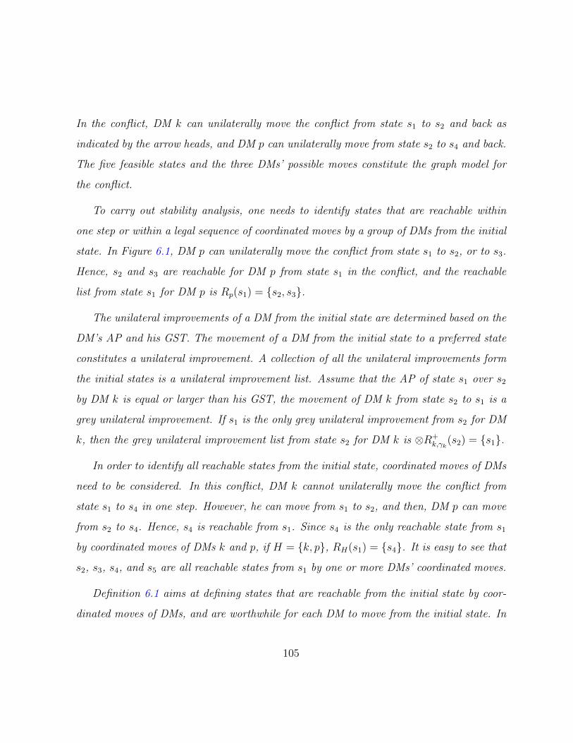
In the conflict, DM k can unilaterally move the conflict from state s1 to s2 and back as

indicated by the arrow heads, and DM p can unilaterally move from state s2 to s4 and back.

The five feasible states and the three DMs’ possible moves constitute the graph model for

the conflict.

To carry out stability analysis, one needs to identify states that are reachable within

one step or within a legal sequence of coordinated moves by a group of DMs from the initial

state. In Figure 6.1, DM p can unilaterally move the conflict from state s1 to s2, or to s3.

Hence, s2 and s3 are reachable for DM p from state s1 in the conflict, and the reachable

list from state s1 for DM p is Rp(s1) = s2, s3.

The unilateral improvements of a DM from the initial state are determined based on the

DM’s AP and his GST. The movement of a DM from the initial state to a preferred state

constitutes a unilateral improvement. A collection of all the unilateral improvements form

the initial states is a unilateral improvement list. Assume that the AP of state s1 over s2

by DM k is equal or larger than his GST, the movement of DM k from state s2 to s1 is a

grey unilateral improvement. If s1 is the only grey unilateral improvement from s2 for DM

k, then the grey unilateral improvement list from state s2 for DM k is ⊗R+k,γk

(s2) = s1.

In order to identify all reachable states from the initial state, coordinated moves of DMs

need to be considered. In this conflict, DM k cannot unilaterally move the conflict from

state s1 to s4 in one step. However, he can move from s1 to s2, and then, DM p can move

from s2 to s4. Hence, s4 is reachable from s1. Since s4 is the only reachable state from s1

by coordinated moves of DMs k and p, if H = k, p, RH(s1) = s4. It is easy to see that

s2, s3, s4, and s5 are all reachable states from s1 by one or more DMs’ coordinated moves.

Definition 6.1 aims at defining states that are reachable from the initial state by coor-

dinated moves of DMs, and are worthwhile for each DM to move from the initial state. In

105

Figure 6.1, if s2 is a grey unilateral improvement for DM k from s1, and s4 is also a grey

unilateral improvement for DM p from s2, then s4 is a grey unilateral improvement from

s1 for DM k and p. Moreover, s4 is the only reachable state from s1 by coordinated moves

of DMs k and p. Hence, if H = k, p, then ⊗R+H,γH

(s1) = s4.

6.1.2 Grey Stabilities Definitions and Equilibria

The stability definitions proposed in Chapter 5 are for a graph model with exact two DMs,

where the opponent of a focal DM is a single DM. When a conflict have more than two

DMs, the opponent of a focal DM is a group (or coalition) of DMs. Hence, Since Nash

stability does not depend on the responses of the opponent(s), the definition of grey Nash

stability for an n-decision Maker (n ≥ 2) graph model is the same as the two-DM case. The

stability concepts of grey general metarationality (GGMR), grey symmetric metarationality

(GSMR) and grey sequential stability (GSEQ) in a n-DM (n ≥ 2) conflict are developed to

deal with stategic conflict with multiple DMs in this chapter. These definitions depend on

GSTs, characteristics of DMs and their corresponding APs (referring to Chpater 5), and

unilateral moves controlled by DMs, GUIs. Note that S = s1, s2, . . . , sm, m > 1 denotes

the set of feasible states and N represents the set of DMs. The formal definitions of the

three grey stabilities for a conflict having multiple DMs are given below.

Definition 6.2 Grey General Metarational (GGMR): A state s ∈ S is grey general

metarational for DM k, denoted by s ∈ SGGMRk , if and only if for every s1 ∈ ⊗R+

k,γk(s)

there exists at least one s2 ∈ RN−k(s1) such that AP k(s2, s) < γk.

If DM k chooses to move from s to a GUI, s1, and the other DMs, N − k, have at least

one unilateral movement from state s1 to a state s2, which is less preferred for DM k than

106

s, based on his preference, characteristics, and satisficing criterion, then the GUI from s

to s1 for DM k is blocked. If every GUI from s by DM k can be blocked by some or all the

other DMs’ unilateral movements, then the state s is GGMR for DM k.

Definition 6.3 Grey Sequentially Stable (GSEQ): A state s ∈ S is grey sequentially

stable for DM k, denoted by s ∈ SGSEQk , if and only if for every s1 ∈ ⊗R+k,γk

(s) there exists

at least one s2 ∈ ⊗R+N−k,γN−k

(s1) such that AP k(s2, s) < γk.

If DM k chooses a GUI s1 from state s to move to, and the other DMs, N − k, have at

least one GUI from state s1 to s2, which is not worthwhile for DM k to move from s based

on his preference, characteristics, and satisficing criterion. If every GUI from s by DM k

can be blocked by some or all the other DMs using GUIs given in Definition 6.1, then the

state s is GSEQ for DM k.

Definition 6.4 Grey Symmetric Metarational (GSMR): A state s ∈ S is grey

symmetric metarational for DM k, denoted by s ∈ SGSMRk , if and only if for every s1 ∈

⊗R+k,γk

(s) there exists at least one s2 ∈ RN−k(s1) such that AP k(s2, s) < γk, and

AP k(s3, s) < γk for all s3 ∈ RN−k(s2).

If DM k chooses to move to a GUI s1 from s, and the other DMs, N−k, have subsequent

unilateral movements from state s1 to s2, which is not worthwhile for DM k from s to

move to, and neither is any unilateral movement of DM k from s2, based on his preference,

characteristics, and satisficing criterion, then the GUI from s to s1 is blocked for DM k. If

every GUI from s by DM k can be blocked in the manner described above, then the state

s is GSMR for DM k.

107

Figure 6.2: Flow Chart for grey-based Graph Model for Conflict Resolution

Definition 6.5 Grey Equilibrium: A state s ∈ S is called a grey equilibrium under a

specific grey stability definition if and only if the state is grey stable for all DMs under that

grey stability definition.

Figure 6.2 is a flowchart that shows the procedure of the grey-based GMCR method-

ology, and explains the relations of definitions provided above. AP for each DM over all

states are determined based on the DM’s characteristic and preferences. The GUI from

the initial states for a DM are identified based on the DM’s AP and GST. The grey stable

states change when the DMs’ GSTs change. Based on the two basic grey stability defini-

tions, grey stable states reflect mainly the possibility of GUIs, which are directly related

to the GST for each DM.

108

6.2 Negotiation of Brownfield Redevelopment

Conflict under Uncertainty

6.2.1 Background of Kaufman Site Redevelopment Conflict

This case study of brownfield redevelopment conflict was proposed by Bernath Walker et al.

(2010). To take uncertain preferences of DMs into consideration, Bashar et al. (2012) used

fuzzy preferences to analyze conflict behaviour and identify possible resolutions to this dis-

pute. In this section, the grey-based preferences are employed to represent multiple DMs’

uncertain preferences with grey numbers, and the grey-based solution concepts designed for

a conflict with multiple DMs are used to analyze the conflict under uncertainty. The defini-

tions of anticipated preferences, grey satisfacing threshold, grey unilateral improvements,

and grey-based stability definitions are originally defined by Kuang et al. (2014a,b).

The Kaufman Footwear factory was a shoe manufacturing company located in Kitch-

ener, Ontario, Canada. The company contributed to the local economy for several decades,

and constituted an important part of the city’s industrial history. As both a brownfield site

and a designated heritage building, the Kaufman footwear factory site has been successfully

redeveloped into residential lofts featuring a high roofline and large windows. This section

examines the successful renovation of the Kaufman Footwear company, simulates inter-

actions of the involved DMs with uncertain preferences, demonstrates the feasibility and

effectiveness of the proposed methodology, and provides valuable insight into the strategic

nature of the brownfield redevelopment conflict.

Bernath Walker et al. (2010) divided the brownfield redevelopment conflict into three

phases: Acquisition, Remediation Selection, and Renovation/Redevelopment. This re-

search focuses on the acquisition conflict. The fundamental components for the conflict

109

are summarized as follows:

• DMs: The graph model for the conflict consists of three DMs: (i) Property Owner

(PO) who aims at selling this property at as high as possible price; (ii) Developer (D)

who tries to make profitable businesses; and (iii) City Government (CG), whose pur-

pose is to increase tax revenue and employment opportunities, and to provide healthy

neighbourhoods, while efficiently and effectively allocating government resources.

• Options: PO has three options: sell the property at a high price, sell low, or walk

away. According to PO’s quotation, D may accept this price or refuse to buy the

property. CG may offer financial and policy oriented incentives or not.

• Feasible States: Feasible states are identified and listed in Table 6.1, in which “Y”

means that the option is chosen by a DM, and “N” means it is rejected. A dash, given

by “-”, means either a “Y” or “N”. In a conflict, a state is formed when each DM

chooses a strategy. For example, the state s2 is formed when PO sells his property

at a high price, while CG refuses to offer related incentives, and D does not accept

this, and waits to see if changes occur. Because each option for the corresponding

DM may be selected or not, in principle, there may be 26 = 64 states in this dispute.

However, some of these states are infeasible. For example, PO cannot choose both to

sell the property at a high price and to walk away at the same time. After removing

infeasible states, thirteen feasible states remain as listed in Table 6.1.

The feasible states describe all possible outcomes of the brownfield redevelopment con-

flict. State s1 is interpreted as the status quo, in which none of the three DMs takes any

action. In states s2 to s6, D doesn’t accept the options provided by PO and CG, and

waits to see if it is possible to gain much more from the conflict. These states can be

110

Table 6.1: DMs, Options, and States in the Acquisition Conflict of Brownfield Redevelop-ment (Modified from (Bernath Walker et al., 2010))

Property Owner (PO)Sell High N Y N N Y N N Y N Y N - -Sell Low N N Y N N Y N N Y N Y - -

Walk N N N N N N N N N N N - YCity Government (CG) Incentives N N N Y Y Y N N N Y Y - -

Developer (D)Buy N N N N N N Y Y Y Y Y - -Walk N N N N N N N N N N N Y -

Feasible States s1 s2 s3 s4 s5 s6 s7 s8 s9 s10 s11 s12 s12

considered as transitional states of this negotiation. States s8, s9, s10, and s11 represent

possible agreements. Another important feature of the conflict is that either D or PO can

choose the option “Walk”, thereby ending the conflict at s12. Hence, the last two states are

the same and marked s12. For example, state s12 is created when PO chooses the option

“Walk” as indicated by the “Y” opposite options 3. The option selections of D and CG

will not affect the conflict as indicated by dashes opposite their options. Meanwhile, s12

can also be created when D chooses “Walk”, and the option selections of PO and CG will

not affect the conflict either.

The directed graph in Figure 6.3 shows available transitions by PO, CG, and D, where

the nodes represent the twelve feasible states, and the color-coded arcs indicate the DMs’

unilateral moves that are controlled by corresponding DMs. For example, CG can unilat-

erally move the conflict from state s1 to s4 and back as indicated by the arrow heads, while

PO can unilaterally move the conflict from state s1 to state s3 and back.

111

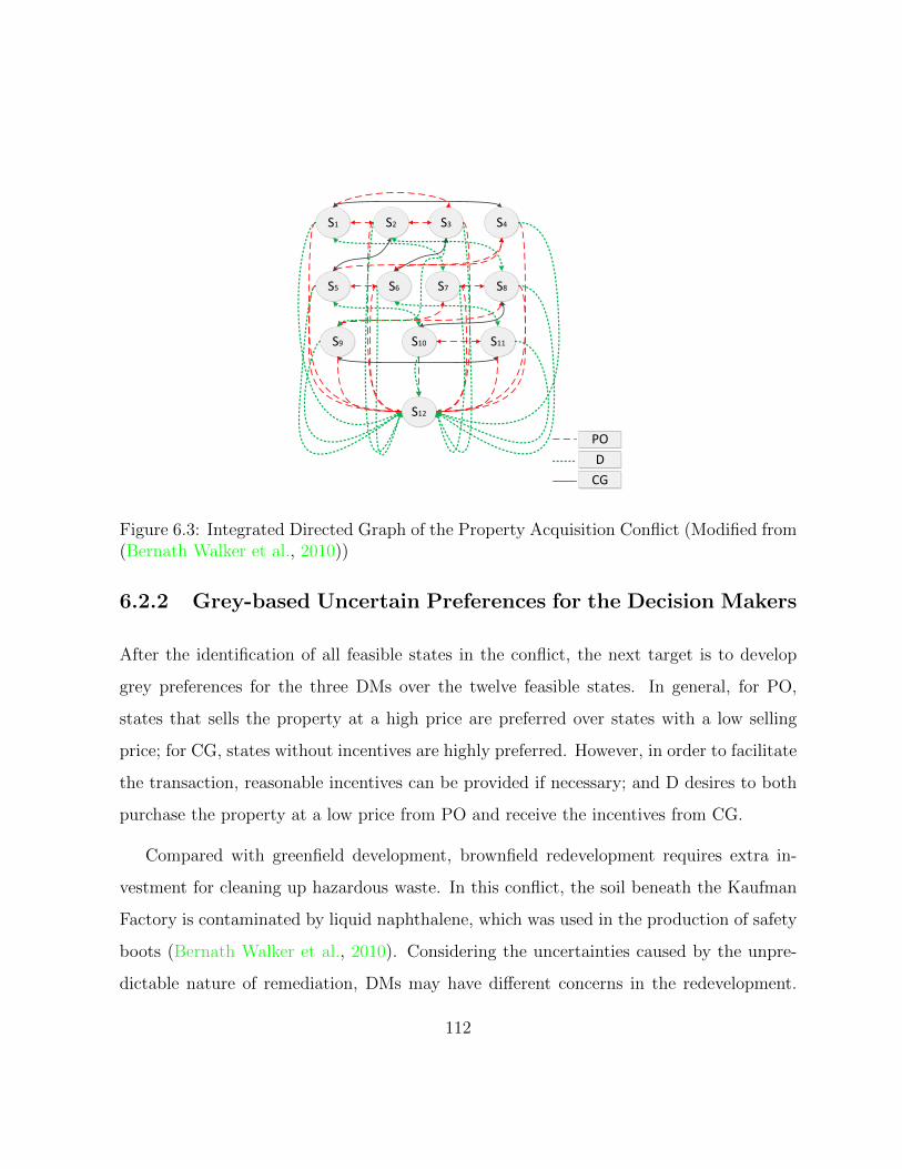
S1 S2 S3 S4

S5 S6 S7 S8

S9 S10 S11

S12

PO

D

CG

Figure 6.3: Integrated Directed Graph of the Property Acquisition Conflict (Modified from(Bernath Walker et al., 2010))

6.2.2 Grey-based Uncertain Preferences for the Decision Makers

After the identification of all feasible states in the conflict, the next target is to develop

grey preferences for the three DMs over the twelve feasible states. In general, for PO,

states that sells the property at a high price are preferred over states with a low selling

price; for CG, states without incentives are highly preferred. However, in order to facilitate

the transaction, reasonable incentives can be provided if necessary; and D desires to both

purchase the property at a low price from PO and receive the incentives from CG.

Compared with greenfield development, brownfield redevelopment requires extra in-

vestment for cleaning up hazardous waste. In this conflict, the soil beneath the Kaufman

Factory is contaminated by liquid naphthalene, which was used in the production of safety

boots (Bernath Walker et al., 2010). Considering the uncertainties caused by the unpre-

dictable nature of remediation, DMs may have different concerns in the redevelopment.

112

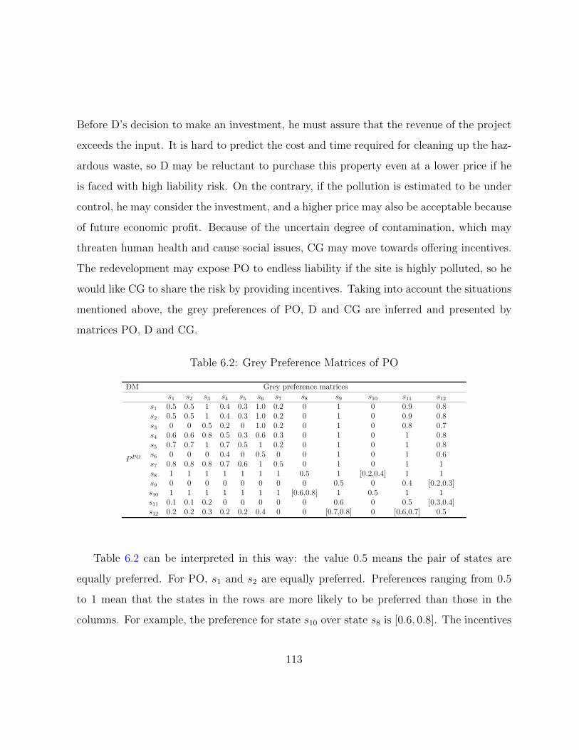
Before D’s decision to make an investment, he must assure that the revenue of the project

exceeds the input. It is hard to predict the cost and time required for cleaning up the haz-

ardous waste, so D may be reluctant to purchase this property even at a lower price if he

is faced with high liability risk. On the contrary, if the pollution is estimated to be under

control, he may consider the investment, and a higher price may also be acceptable because

of future economic profit. Because of the uncertain degree of contamination, which may

threaten human health and cause social issues, CG may move towards offering incentives.

The redevelopment may expose PO to endless liability if the site is highly polluted, so he

would like CG to share the risk by providing incentives. Taking into account the situations

mentioned above, the grey preferences of PO, D and CG are inferred and presented by

matrices PO, D and CG.

Table 6.2: Grey Preference Matrices of PO

DM Grey preference matricess1 s2 s3 s4 s5 s6 s7 s8 s9 s10 s11 s12

P PO

s1 0.5 0.5 1 0.4 0.3 1.0 0.2 0 1 0 0.9 0.8s2 0.5 0.5 1 0.4 0.3 1.0 0.2 0 1 0 0.9 0.8s3 0 0 0.5 0.2 0 1.0 0.2 0 1 0 0.8 0.7s4 0.6 0.6 0.8 0.5 0.3 0.6 0.3 0 1 0 1 0.8s5 0.7 0.7 1 0.7 0.5 1 0.2 0 1 0 1 0.8s6 0 0 0 0.4 0 0.5 0 0 1 0 1 0.6s7 0.8 0.8 0.8 0.7 0.6 1 0.5 0 1 0 1 1s8 1 1 1 1 1 1 1 0.5 1 [0.2,0.4] 1 1s9 0 0 0 0 0 0 0 0 0.5 0 0.4 [0.2,0.3]s10 1 1 1 1 1 1 1 [0.6,0.8] 1 0.5 1 1s11 0.1 0.1 0.2 0 0 0 0 0 0.6 0 0.5 [0.3,0.4]s12 0.2 0.2 0.3 0.2 0.2 0.4 0 0 [0.7,0.8] 0 [0.6,0.7] 0.5

Table 6.2 can be interpreted in this way: the value 0.5 means the pair of states are

equally preferred. For PO, s1 and s2 are equally preferred. Preferences ranging from 0.5

to 1 mean that the states in the rows are more likely to be preferred than those in the

columns. For example, the preference for state s10 over state s8 is [0.6, 0.8]. The incentives

113

offered by CG cannot change the profit accrued by PO from selling the property at a high

price, but it can help to convince D to accept the price, thereby facilitating the transaction.

On the contrary, preferences ranging from 0 to 0.5 mean the states in the rows are likely

less preferred than those in the columns. The value of 1 means preferred, and 0 means not

preferred. For example, state s8 is strictly preferred to s9, because PO always prefers to

sell the property at a high price.

Table 6.3: Grey Preference Matrices of CG

DM Grey preference matricess1 s2 s3 s4 s5 s6 s7 s8 s9 s10 s11 s12

PCG

s1 0.5 0.6 0.4 0.3 0.4 0.2 0.3 0 0 0 0 1s2 0.4 0.5 0.3 0.2 0.4 0.2 0.4 0 0 0 0 1s3 0.6 0.7 0.5 0.4 0.6 0.4 0.4 0 1 0 0 1s4 0.7 0.8 0.6 0.5 0.6 0.3 0.4 0 1 0 0 1s5 0.6 0.6 0.4 0.4 0.5 0.2 0.3 0 1 0 0 1s6 0.8 0.8 0.6 0.7 0.8 0.5 0.5 0 1 0 0 1s7 0.7 0.6 0.6 0.6 0.7 0.5 0.5 0 1 0 0 1s8 1 1 1 1 1 1 1 0.5 [0.3,0.5] [0.4,0.5][0.6,0.8] [0.3,0.5][0.7,0.9] 1s9 1 1 1 1 1 1 1 [0.5,0.7] 0.5 [0.1,0.4][0.6,0.7] [0.4,0.5][0.6,0.8] 1s10 1 1 1 1 1 1 1 [0.2,0.4][0.5,0.6] [0.3,0.4][0.6,0.9] 0.5 [0.3,0.5] 1s11 1 1 1 1 1 1 1 [0.1,0.3][0.5,0.7] [0.2,0.4][0.5,0.6] [0.5,0.7] 0.5 1s12 0 0 0 0 0 0 0 0 0 0 0 0.5

Table 6.3 shows the uncertain preferences of CG over the feasible states. CG is eager

to see that PO and D reach an agreement, and that the Kaufman Factory brownfield be

remediated. In this way, threats of hazardous waste will be removed and tax income will

increase with the new development. As a result, states s8 to s10 are highly preferred over

the others. Because CG cares about the success of the transaction, it prefers that PO sells

the property at a low price, which makes it easier for D to accept. Then, s8 is less preferred

than s9, and s11 is less preferred than s12. Whether CG would like to offer extra incentives

also depends on the degree of pollution. If the property is highly polluted, leading to

potential liability risk and extra remediation costs, CG needs to take up the duties and

share the responsibilities with D, otherwise D will not be engaged in this situation; if the

114

property is only somewhat polluted, CG hopes D can handle it. Hence, combinations of

intervals are used to represent preference relations between s9 and s10, s8 and s10, s8 and

s11 as well as s9 and s11. States s1 to s7 indicate that an agreement cannot be reached. In

these situations, CG prefers that PO sells the property at a low price and offers reasonable

incentives to persuade D to accept the deal. Uncertain preferences are applied to represent

the CG’s concerns.

Table 6.4: Grey Preference Matrices of D

DM Grey preference matricess1 s2 s3 s4 s5 s6 s7 s8 s9 s10 s11 s12

PD

s1 0.5 0.5 0 0 0 0 0.8 1 0 0 0 1s2 0.5 0.5 0 0 0 0 0.7 1 0 0 0 1s3 1 1 0.5 [0.6,0.7] [0.5,0.7] 0 1 1 0 0 0 1s4 1 1 [0.3,0.4] 0.5 0.5 0 1 1 0 0 0 1s5 1 1 [0.3,0.5] 0.5 0.5 0 1 1 0 0.2 0 1s6 1 1 1 1 1 0.5 1 1 1 1 0 1s7 0.2 0.3 0 0 0 0 0.5 1 0 0 0 1s8 0 0 0 0 0 0 0 0.5 0 0 0 0s9 1 1 1 1 1 0 1 1 0.5 [0.5,0.7] 0 1s10 1 1 1 1 0.8 0 1 1 [0.3,0.5] 0.5 0 1s11 1 1 1 1 1 1 1 1 1 1 0.5 1s12 0 0 0 0 0 0 0 1 0 0 0 0.5

Considering the convenient location of the property and the prosperous future of the

community, the redevelopment of this area is attractive to D. s11 is obviously the most

preferred state for D, because he buys the property at a low price and also gets incentives

from CG. The uncertain preference for state s9 over s10 depends on whether the lower price

or the incentives are more beneficial. Generally, the incentives provided by CG are indirect,

like fee rebates and tax deduction, so a lower price from PO is likely more preferred. On

the contrary, the least preferred situation for D is PO insisting on selling at a high price

with no support offered from CG. In this circumstance, D might choose to back out of the

115

Table 6.5: Grey Relative Preference Matrices of PO

DM Grey Relative certainty of Preference for POs1 s2 s3 s4 s5 s6 s7 s8 s9 s10 s11 s12

rPO

s1 0 0 1 -0.2 -0.4 1 -0.6 -1 1 -1 0.8 0.6s2 0 0 1 -0.2 -0.4 1 -0.6 -1 1 -1 0.8 0.6s3 -1 -1 0 -0.6 -1 1 -0.6 -1 1 -1 0.6 0.4s4 0.2 0.2 0.6 0 -0.4 0.2 -0.4 -1 1 -1 1 0.6s5 0.4 0.4 1 0.4 0 1 -0.6 -1 1 -1 1 0.6s6 -1 -1 -1 -0.2 -1 0 -1 -1 1 -1 1 0.2s7 0.6 0.6 0.6 0.4 0.6 1 0 -1 1 -1 1 1s8 1 1 1 1 1 1 1 0 1 [-0.6,-0.2] 1 1s9 -1 -1 -1 -1 -1 -1 -1 -1 0 -1 -0.2 [-0.6,-0.4]s10 1 1 1 1 1 1 1 [0.2,0.6] 1 0 1 1s11 -0.8 -0.8 -0.6 -1 -1 -1 -1 -1 -0.6 -1 0 [-0.4,0.2]s12 -0.6 -0.6 -0.4 -0.6 -0.6 -0.2 -1 -1 [0.4,0.6] -1 [0.2,0.4] 0

negotiation. For the middle states from s1 to s7, D is indifferent whether PO refuses to

sell or insists on a high price, so s1 is equally preferred to s2. The preference for s3 over s5

is similar to that for s9 over s10. s6 is highly preferred, because D already gets a desirable

outcome, but is still in negotiation with PO and CG with the purpose of achieving more

benefits. However, s7, in which D shows his sincerity but receives no response from CG

and PO, is less preferred.

Based on the inferred grey preferences, the grey relative certainty of preference (GRCP)

for PO, CG, and D can be calculated according to (5.3), separately. After the transfor-

mation, the uncertain preference for each of the three DMs is represented by GRCP. The

value 0 means the pair of states are equally preferred. The positive preferences, ranging

from 0 to 1 mean that the states in the rows are likely more preferred than those in the

columns. On the contrary, the negative preferences, ranging from -1 to 0 mean the states

in the rows are likely less preferred than those in the columns. The value of -1 means not

preferred, and that of 1 means preferred. Compared with grey preferences, it is easier to

tell the preference relationship over feasible states through the GRCP.

116

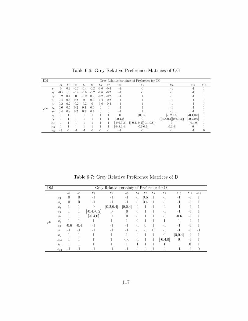
Table 6.6: Grey Relative Preference Matrices of CG

DM Grey Relative certainty of Preference for CGs1 s2 s3 s4 s5 s6 s7 s8 s9 s10 s11 s12

rCG

s1 0 0.2 -0.2 -0.4 -0.2 -0.6 -0.4 -1 -1 -1 -1 1s2 -0.2 0 -0.4 -0.6 -0.2 -0.6 -0.2 -1 -1 -1 -1 1s3 0.2 0.4 0 -0.2 0.2 -0.2 -0.2 -1 1 -1 -1 1s4 0.4 0.6 0.2 0 0.2 -0.4 -0.2 -1 1 -1 -1 1s5 0.2 0.2 -0.2 -0.2 0 -0.6 -0.4 -1 1 -1 -1 1s6 0.6 0.6 0.2 0.4 0.6 0 0 -1 1 -1 -1 1s7 0.4 0.2 0.2 0.2 0.4 0 0 -1 1 -1 -1 1s8 1 1 1 1 1 1 1 0 [0,0.4] [-0.2,0.6] [-0.4,0.8] 1s9 1 1 1 1 1 1 1 [-0.4,0] 0 [-0.8,0.1][0.2,0.4] [-0.2,0.6] 1s10 1 1 1 1 1 1 1 [-0.6,0.2] [-0.4,-0.2][-0.1,0.8] 0 [-0.4,0] 1s11 1 1 1 1 1 1 1 [-0.8,0.4] [-0.6,0.2] [0,0.4] 0 1s12 -1 -1 -1 -1 -1 -1 -1 -1 -1 -1 -1 0

Table 6.7: Grey Relative Preference Matrices of D

DM Grey Relative certainty of Preference for Ds1 s2 s3 s4 s5 s6 s7 s8 s9 s10 s11 s12

rD

s1 0 0 -1 -1 -1 -1 0.6 1 -1 -1 -1 1s2 0 0 -1 -1 -1 -1 0.4 1 -1 -1 -1 1s3 1 1 0 [0.2,0.4] [0,0.4] -1 1 1 -1 -1 -1 1s4 1 1 [-0.4,-0.2] 0 0 0 1 1 -1 -1 -1 1s5 1 1 [-0.4,0] 0 0 -1 1 1 -1 -0.6 -1 1s6 1 1 1 1 1 0 1 1 1 1 -1 1s7 -0.6 -0.4 -1 -1 -1 -1 0 1 -1 -1 -1 1s8 -1 -1 -1 -1 -1 -1 -1 0 -1 -1 -1 -1s9 1 1 1 1 1 -1 1 1 0 [0,0.4] -1 1s10 1 1 1 1 0.6 -1 1 1 [-0.4,0] 0 -1 1s11 1 1 1 1 1 1 1 1 1 1 0 1s12 -1 -1 -1 -1 -1 -1 -1 1 -1 -1 -1 0

117

6.2.3 Stability Analysis of the Brownfield Redevelopment

Conflict

Grey stability analysis can be carried out only after DMs’ characteristics have been iden-

tified. In this conflict, after the bankruptcy of Kaufman Footwear, PO is eager to sell the

property at a high price; D needs a comprehensive estimate in order to make a wise choice;

and CG is neutral about incentives. Hence, it is reasonable to assume that the character-

istics of these three DMs are: PO optimistic, D pessimistic, and CG neutral. Based on

the characteristics of the DMs, the AP for each DM can be calculated according to (5.5),

(5.6), and (5.7), and the results are as shown in Table 6.8.

In the conflict, based on the unilateral moves of DMs in the conflict, shown in Figure

6.3, the Figures 6.4, 6.5, and 6.6 are drawn to reflect how GUIs for each DM depend on

the GSTs. In the directed graph shown in Figure 6.4, the color-coded arrows represent

unilateral improvements of PO holding different GSTs, and indifferent states are connected

by a double black line. For example, the blue arrows represent unilateral improvements of

PO when his GST is in the range (0.2, 0.4], such as s5 is a GUI from state s4 for him. PO’s

GST is classified into 3 different ranges according to his unilateral moves (see Figure 6.3),

and anticipated preferences, which are determined by his characteristic and grey relative

preferences, (see Table 6.5). Note that classifying DM’s GST is to facilitate a grey stability

analysis. For instance, when the GST falls into a lower range, the GUIs requiring higher

range of GST are also valid. In particular, if PO’s GST is equal to 0.1, the states directed

by black, blue and red are all GUIs form their corresponding initial vertices. The directed

graph indicates that the GUIs of PO can change a great deal when his GST changes.

In the directed graph shown in Figure 6.4, the arrows with different colours represent

unilateral improvements of PO holding different GSTs, and indifferent states are connected

118

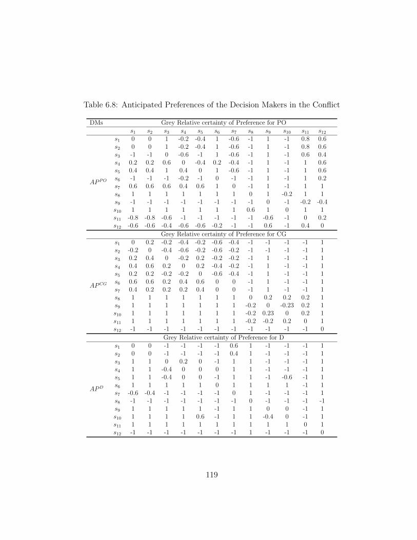
Table 6.8: Anticipated Preferences of the Decision Makers in the Conflict

DMs Grey Relative certainty of Preference for POs1 s2 s3 s4 s5 s6 s7 s8 s9 s10 s11 s12

AP PO

s1 0 0 1 -0.2 -0.4 1 -0.6 -1 1 -1 0.8 0.6s2 0 0 1 -0.2 -0.4 1 -0.6 -1 1 -1 0.8 0.6s3 -1 -1 0 -0.6 -1 1 -0.6 -1 1 -1 0.6 0.4s4 0.2 0.2 0.6 0 -0.4 0.2 -0.4 -1 1 -1 1 0.6s5 0.4 0.4 1 0.4 0 1 -0.6 -1 1 -1 1 0.6s6 -1 -1 -1 -0.2 -1 0 -1 -1 1 -1 1 0.2s7 0.6 0.6 0.6 0.4 0.6 1 0 -1 1 -1 1 1s8 1 1 1 1 1 1 1 0 1 -0.2 1 1s9 -1 -1 -1 -1 -1 -1 -1 -1 0 -1 -0.2 -0.4s10 1 1 1 1 1 1 1 0.6 1 0 1 1s11 -0.8 -0.8 -0.6 -1 -1 -1 -1 -1 -0.6 -1 0 0.2s12 -0.6 -0.6 -0.4 -0.6 -0.6 -0.2 -1 -1 0.6 -1 0.4 0

Grey Relative certainty of Preference for CG

APCG

s1 0 0.2 -0.2 -0.4 -0.2 -0.6 -0.4 -1 -1 -1 -1 1s2 -0.2 0 -0.4 -0.6 -0.2 -0.6 -0.2 -1 -1 -1 -1 1s3 0.2 0.4 0 -0.2 0.2 -0.2 -0.2 -1 1 -1 -1 1s4 0.4 0.6 0.2 0 0.2 -0.4 -0.2 -1 1 -1 -1 1s5 0.2 0.2 -0.2 -0.2 0 -0.6 -0.4 -1 1 -1 -1 1s6 0.6 0.6 0.2 0.4 0.6 0 0 -1 1 -1 -1 1s7 0.4 0.2 0.2 0.2 0.4 0 0 -1 1 -1 -1 1s8 1 1 1 1 1 1 1 0 0.2 0.2 0.2 1s9 1 1 1 1 1 1 1 -0.2 0 -0.23 0.2 1s10 1 1 1 1 1 1 1 -0.2 0.23 0 0.2 1s11 1 1 1 1 1 1 1 -0.2 -0.2 0.2 0 1s12 -1 -1 -1 -1 -1 -1 -1 -1 -1 -1 -1 0

Grey Relative certainty of Preference for D

APD

s1 0 0 -1 -1 -1 -1 0.6 1 -1 -1 -1 1s2 0 0 -1 -1 -1 -1 0.4 1 -1 -1 -1 1s3 1 1 0 0.2 0 -1 1 1 -1 -1 -1 1s4 1 1 -0.4 0 0 0 1 1 -1 -1 -1 1s5 1 1 -0.4 0 0 -1 1 1 -1 -0.6 -1 1s6 1 1 1 1 1 0 1 1 1 1 -1 1s7 -0.6 -0.4 -1 -1 -1 -1 0 1 -1 -1 -1 1s8 -1 -1 -1 -1 -1 -1 -1 0 -1 -1 -1 -1s9 1 1 1 1 1 -1 1 1 0 0 -1 1s10 1 1 1 1 0.6 -1 1 1 -0.4 0 -1 1s11 1 1 1 1 1 1 1 1 1 1 0 1s12 -1 -1 -1 -1 -1 -1 -1 1 -1 -1 -1 0

119

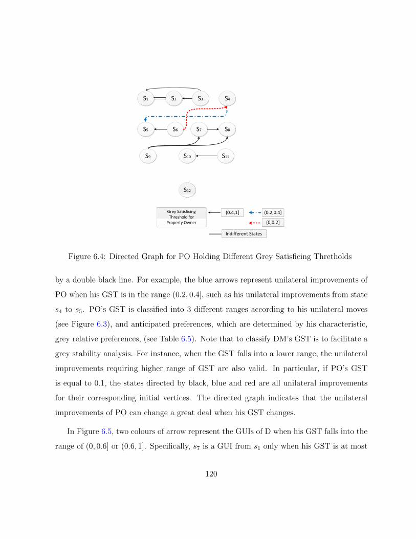
S1 S2 S3 S4

S5 S6 S7 S8

S9 S10 S11

S12

(0.2,0.4]

(0,0.2]

(0.4,1]Grey Satisficing Threshold for

Property Owner

Indifferent States

Figure 6.4: Directed Graph for PO Holding Different Grey Satisficing Thretholds

by a double black line. For example, the blue arrows represent unilateral improvements of

PO when his GST is in the range (0.2, 0.4], such as his unilateral improvements from state

s4 to s5. PO’s GST is classified into 3 different ranges according to his unilateral moves

(see Figure 6.3), and anticipated preferences, which are determined by his characteristic,

grey relative preferences, (see Table 6.5). Note that to classify DM’s GST is to facilitate a

grey stability analysis. For instance, when the GST falls into a lower range, the unilateral

improvements requiring higher range of GST are also valid. In particular, if PO’s GST

is equal to 0.1, the states directed by black, blue and red are all unilateral improvements

for their corresponding initial vertices. The directed graph indicates that the unilateral

improvements of PO can change a great deal when his GST changes.

In Figure 6.5, two colours of arrow represent the GUIs of D when his GST falls into the

range of (0, 0.6] or (0.6, 1]. Specifically, s7 is a GUI from s1 only when his GST is at most

120

S1 S2 S3 S4

S5 S6 S7 S8

S9 S10 S11

S12

(0.6,1]

(0,0.6]

Grey Satistisficing Threshold for

Developer

Figure 6.5: Directed Graph for D Holding Different Grey Satisficing Thretholds

0.6, (see Table 6.7); for the other GUIs, indicated by red arrows, the relationship between

each pair of states is a strict preference. Hence, these GUIs do not change with D’s GST.

D is concerned about his investment, and will move only to states that are preferred with

high confidence, which is consistent with his characteristic. In Figure 6.6, GUIs for CG

are indicated by blue and purple arrows according to the GST. These GUIs are valid only

when CG’s GST is relatively low.

After the identification of GUIs for PO, D and CG, respectively, stable states of the

Kaufman brownfield redevelopment conflict under uncertainty can be determined. Three

sets of GSTs for PO, D and CG are assumed, which are 0.8, 1, 0.6, 0.5, 0.8, 0.4, 0.2,

0.6, 0.2. The stability results based on the stability definitions are displayed in Table 6.9.

In this table, a state that is stable for PO, D and CG is marked√

under corresponding

grey stability definitions, while GE indicates that the state is stable for all DMs.

121

S1 S2 S3 S4

S5 S6 S7 S8

S9 S10 S11

S12

(0.2,0.4]

(0,0.2]

Grey Satistisficing Threshold for

City Government

Figure 6.6: Directed Graph for CG Holding Different Grey Satisficing Thretholds

Note that both D and PO can unilaterally abandon the transaction, and any unilateral

move for PO or D to s12 is irreversible, so the state s12 is grey Nash stable for all DMs,

thereby grey sequentially stable. Moreover, a GUI from any state except for s12 of any DM

can be sanctioned by the other two DMs through moving the conflict to state s12. Hence,

all states for all the DMs are grey symmetric metarational and grey general metarational

(Kuang et al., 2014a). Thus, these two types of stability definitions are meaningless in the

conflict analysis, and are not discussed in this case study.

In this conflict, the focal DM’s GUIs from an initial state can only be sanctioned by

the other DMs’ GUIs. In order to interpret the stability results, GUIs for the DMs in three

sets of GSTs are drawn as shown in Figures 6.7, 6.8 and 6.9. In these Figures, a GUI from

a initial state is directed by a black arrow. The GUIs from corresponding initial states

within green frames opposite a DM can be sanctioned by the other DMs’ GUIs, which are

connected by red arrows. Then the initial states are called grey sequentially stable. For

122

Table 6.9: Stability Results for Brownfield Redevelopment Conflict under Uncertainty

GST: Property Owner = 0.1, Developer = 0.6, City Government = 0.2States s1 s2 s3 s4 s5 s6 s7 s8 s9 s10 s11 s12

GRPO

√ √ √ √ √ √

D√ √ √ √ √ √ √

CG√ √ √ √ √ √ √

GSEQPO

√ √ √ √ √ √ √

D√ √ √ √ √ √ √ √ √

CG√ √ √ √ √ √ √ √ √

GE√ √ √

GST: Property Owner = 0.9, Developer= 0.6, City Government = 0.2

GRPO

√ √ √ √ √ √

D√ √ √ √ √ √ √ √ √

CG√ √ √ √ √ √ √ √ √ √

GSEQPO

√ √ √ √ √ √ √

D√ √ √ √ √ √ √ √ √

CG√ √ √ √ √ √ √ √ √ √

GE√ √ √ √

GST: Property Owner = 0.8, Developer = 1, City Government = 0.6

GRPO

√ √ √ √ √ √ √

D√ √ √ √ √ √ √ √ √

CG√ √ √ √ √ √ √ √ √ √ √

GSEQPO

√ √ √ √ √ √ √

D√ √ √ √ √ √ √ √ √ √

CG√ √ √ √ √ √ √ √ √ √ √

GE√ √ √ √ √

123

example, in Figure 6.7, if D unilaterally moves the conflict from s3 to s9, then PO would

prefer to move from s9 to s7 or s8, both of which are less preferred than s3 by D. Hence

s3 is grey sequentially stable for D. Note that the states that do not have GUIs are grey

Nash stable for the DM, such as s1 and s2 for PO.

S3

S9

S11

S2

S1

S4

S5

S6

S5

S4

S7

S8 S7

S8

S10

S3 S5 S6

S11

S8

S2

S10

S9

S7

S1

S1

S4

S2

S5

S3

S6 S8

S10 S11

S9

PropertyOwner

Developer

CityGovernment

Figure 6.7: Grey Unilateral Improvements and Potential Sanctions (GST: PO = 0.1, D =0.6, CG = 0.2)

The first situation (GST: PO = 0.1, D = 0.6, CG = 0.2), as shown in Figure 6.7, has

the most GUIs for each DM, because of their corresponding lowest GSTs. Three states

s5, s10, and s12 are equilibria. Among them, s5 and s12 are grey Nash stable, while s10 is

grey sequentially stable. Specifically, none of the DMs has GUIs from state s5 and s12. s10

is grey Nash stable for PO and D, and grey sequentially stable for CG. If CG chooses to

unilaterally move from s10 to s8, then D can unilaterally move the conflict from s8 to s2.

However, according to the anticipated preferences of CG and its GST, s2 is less preferred

than s10. To avoid ruining the transaction, CG will stay in state s10.

In the second situation (GST: PO = 0.9, D = 0.6, CG = 0.2), as shown in Figure 6.8,

the number of PO’s GUIs decreases when his GST increases, some of PO’s GUIs, such

as his movements from s4 to s5, and from s6 to s4, in the first situation are no longer

124

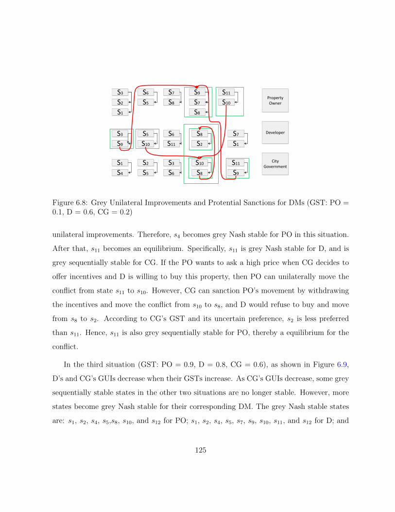
S3

S9

S11

S2

S1

S6

S5

S7

S8 S7

S8

S10

S3 S5 S6

S11

S8

S2

S10

S9

S7

S1

S1

S4

S2

S5

S3

S6 S8

S10 S11

S9

PropertyOwner

Developer

CityGovernment

Figure 6.8: Grey Unilateral Improvements and Protential Sanctions for DMs (GST: PO =0.1, D = 0.6, CG = 0.2)

unilateral improvements. Therefore, s4 becomes grey Nash stable for PO in this situation.

After that, s11 becomes an equilibrium. Specifically, s11 is grey Nash stable for D, and is

grey sequentially stable for CG. If the PO wants to ask a high price when CG decides to

offer incentives and D is willing to buy this property, then PO can unilaterally move the

conflict from state s11 to s10. However, CG can sanction PO’s movement by withdrawing

the incentives and move the conflict from s10 to s8, and D would refuse to buy and move

from s8 to s2. According to CG’s GST and its uncertain preference, s2 is less preferred

than s11. Hence, s11 is also grey sequentially stable for PO, thereby a equilibrium for the

conflict.

In the third situation (GST: PO = 0.9, D = 0.8, CG = 0.6), as shown in Figure 6.9,

D’s and CG’s GUIs decrease when their GSTs increase. As CG’s GUIs decrease, some grey

sequentially stable states in the other two situations are no longer stable. However, more

states become grey Nash stable for their corresponding DM. The grey Nash stable states

are: s1, s2, s4, s5,s8, s10, and s12 for PO; s1, s2, s4, s5, s7, s9, s10, s11, and s12 for D; and

125

S3

S9

S11

S2

S1

S6

S5

S7

S8 S7

S8

S3 S6

S11

S8

S2

S10

S9

S1

S4

PropertyOwner

Developer

CityGovernment

Figure 6.9: Grey Unilateral Improvements and Protential Sanctions for DMs (GST: PO =0.9, D = 0.8, CG = 0.6)

all states except s1 for CG. Hence, s1, s2, s4, s5, s10, and s12 are equilibria for the conflict

in this situation.

6.2.4 Status Quo Analysis

Through the stability analysis, equilibria have been found in the graph model for brown-

field redevelopment conflict, when DMs’ uncertain preferences are considered. Among

them, two states s10 and s11, indicating the completion of the transaction, are found to be

equilibria under corresponding situations. A status quo analysis is carried out, in order to

dynamically examine whether they are reachable from the status quo in reality, to access

which equilibrium is more likely to happen, and to explore how these equilibria can be

reached, thereby providing insights of the conflict on how to achieve desirable stable states

for DMs. In this conflict, s1 is the status quo state, and the potential evolutions involve

moves from s1 to equilibria s10 and s11, as shown in Table 6.10.

Table 6.10 shows how equilibria s10 and s11 are reached from status quo s1 through

126

Table 6.10: Status Quo Analysis

DMs Status Quo Transitional states Equilibria

PON N −−−−→ Y YN N N NN N N N

CG N −−−−→ Y Y Y

DN N N −−−−→ YN N N N

States s1 s4 s5 s10

PON N N NN −−−−→ Y Y YN N N N

CG N N −−−−→ Y Y

DN N N −−−−→ YN N N N

States s1 s3 s6 s11

transitional states by corresponding DMs. Based on the stability analysis, the focal DM’s

GUIs from a initial state can be sanctioned only by the other DMs’ GUIs, which means

none of the DMs will sanction the other DMs’ GUIs by sacrificing his benefits. s10 is

reachable only when s4 is a GUI from s1 for CG, s5 is a GUI from s4 for PO, and s10

is a GUI from s5 for D. In this circumstance, according to the directed graphs for DMs

holding different GSTs, shown in Figures 6.4, 6.5 and 6.6, the GSTs for DMs should be

0 < γCG 6 0.2, 0 < γPO 6 0.4, and 0 < γD 6 0.6, respectively. To achieve mutual benefit

results, all DMs need to compromise their GSTs, and CG plays a key role in facilitating

the transaction. However, s11 is hard to reach. Even though s6 can be a GUI from s3

for CG when 0 < γCG 6 0.2, and s11 is a GUI from s6 for D, s3 is not preferred by PO

compared with s1 who will not reduce the price of the property at the beginning of the

conflict, unless he is extremely short of money. As a result, s10 is more likely to happen.

127

6.3 Conclusions

This research, using grey numbers to express uncertain preferences of DMs, aims to de-

fine grey-based stability concepts and corresponding equilibria within the GMCR struc-

ture when multiple DMs are involved in a conflict, thereby extending the graph model

methodology. These definitions can account for missing preference information in a mul-

tiple participant-multiple objective decision model, and therefore, provide more realistic

resolutions to a conflict being studied in the face of uncertainty.

This methodology is applied to a brownfield redevelopment conflict that occurred in

Kitchener, Ontario, Canada, in which DMs have uncertain preferences. The directed graphs

for DMs holding different GSTs are drawn. Based on three sets of GSTs for DMs, GUIs

and potential sanctions for each DM are also provided, and then stability results are cal-

culated according to two types of grey stability concepts (grey Nash stability, and grey

sequential stability). Subsequently, further interpretation of these equilibria is given, with

an explanation of how equilibria will change when DMs’ GSTs are altered. A status quo

analysis is also carried out to assess which equilibria are reachable from the status quo and

which one is most likely to occur in the actual conflict.

128

Chapter 7

Contributions and Future Research

This research presents the concept of grey numbers, and then integrates them with tech-

niques in the fields of Multiple Criteria Decision Analysis (MCDA) and Graph Model for

Conflict Resolution (GMCR). Two methodologies, grey-based PROMETHEE II and grey-

based GMCR, are put forward, and some practical applications are investigated using these

novel techniques. The main contributions and suggestions for future research of this thesis

are summarised in the following two sections.

7.1 Main Contributions

The key contributions of this thesis are summarised as follows:

• In Chapter 2, the classification of main stream MCDA methodologies and some

representative techniques are presented. Subsequently, the decision structure and

calculation processes for PROMETHEE II are explained in detail. Moreover, a sys-

129

tematic introduction of fundamental concepts and theorems of grey systems theory

are given, followed by a mathematical illustration of grey relational analysis.

• The grey-based PROMETHEE II methodology is put forward in Chapter 3 to handle

MCDA problems with ill-defined information, using the concept of grey numbers to

represent uncertain input data, and employing linguistic expressions combined with

grey numbers to express DMs’ preferences on alternatives. In the methodology, a

basic structure of a grey decision system is constructed, in which multiple alternatives,

criteria and DMs are taken into account. Then, calculation processes are introduced

to normalize performance of alternatives on both quantitative and qualitative criteria.

In addition, a preference measurement function is designed to evaluate the preference

degree of one alternative over another, and the PROMETHEE II method is modified

for accomplishing ranking alternatives with normalized performances.

• A case study in Chapter 3 regarding the evaluation of source water protection strate-

gies in Region of Waterloo, Ontario, Canada, is introduced to demonstrate how to

apply the grey-based PROMETHEE II methodology. The results show that the

methodology can provide a complete ranking order of alternatives having uncertain

information.

• In Chapter 4, mathematical definitions and solution concepts within the context

of GMCR are summarised. To illustrate the process of employing conflict analysis

within the framework of graph model, a case study regarding a conflict over water

use and oil sands development in the Athabasca River among three DMs: Oils Sands

Companies, Local Government, and NGOs, is put forward. Through a thorough sta-

bility analysis, the results indicate that it is possible to balance oil sands development

and environmental protection, whereby the sustainable development of the oil sands

130

industry requires the collaboration of all DMs.

• A new preference structure based on general grey numbers is introduced in Chapter

5. A generalized grey number with values ranging from 0 to 1, may represent a

preference degree, interval of preference degrees, or combinations thereof, and this

concept is used to capture preference uncertainty between two states by a DM. The

grey preference structure allows DMs to describe preferences with generalized grey

numbers, in addition to strict preference and indifference. A number of grey-based

concepts within the framework of GMCR are formally defined, such as grey preference

degrees, grey relative certainty of preferences, anticipated preferences, grey satisficing

threshold, and grey unilateral improvements.

• Grey-based stability definitions based on the grey preference structure are put for-

ward to identify stable states or equilibria when two DMs are involved in a conflict

with uncertain preferences in Chapter 5. Specifically, grey Nash stability, grey gen-

eral metarationality, grey symmetric metarationality, and grey sequential stability

are formally defined along with associated theorems, and corresponding explanations

are provided. Furthermore, a case study involving a sustainable development conflict

under uncertainty, is developed to illustrate how this methodology can be utilized to

analyze a practical conflict when DMs have uncertain preferences.

• In Chapter 6, the grey-based GMCR methodology is further explored to deal with

conflicts having two or more DMs. In this circumstance, coordinated unilateral moves

and unilateral improvements of multiple DMs have been defined under the grey-based

uncertain preference structure. Then the aforementioned four kinds of grey stabilities

are modified to be suitable for employment with a grey-based conflict model having

two or more DMs. The feasibility of this methodology is verified through a case study

131

regarding negotiations in a brownfield redevelopment conflict under uncertainty in

Kitchener, Ontario, Canada.

In summary, this thesis lays down the foundation of new methodologies for handling

uncertain decision problems within the frameworks of MCDA and GMCR. The research

involves both theoretical developments coupled with real-world case studies.

7.2 Future Research Plan

The methodologies proposed in this thesis can be further refined and expanded in the fields

of MCDA and GMCR. Some possible directions for future research are as follows:

• Grey-based methods can be developed for screening, and eliminating alternatives in

the field of MCDA based on the fundamental concepts of grey systems theory.

• In the thesis, a grey preference structure was incorporated into GMCR, thereby

allowing DMs to represent their preferences in a flexible way. However, it raises

complexity in calculating grey-based stable states. Accordingly, a decision support

system should be developed for permitting convenient implementation by both prac-

titioners and researchers.

• The grey preference structure could be employed to help understand processes of

group decision and negotiation.

• The grey-based GMCR methodology focuses only on the four basic stability defini-

tions. Complex solution concepts, such as limited move stability and non-myopic

stability, may be further studied in the future from a grey perspective.

132

• The presented methodologies can be further refined and modified by analysing more

real-world applications in an attempt to provide more insights and reasonable sug-

gestions for DMs to consider.

133

References

Agell, N., Sanchez, M., Prats, F., and Rosello, L. (2012). Ranking multi-attribute alterna-tives on the basis of linguistic labels in group decisions. Information Sciences, 209:49–60.

Alberta Department of Energy (2013). Talk about oil sands. Technical report. Available:http://www.energy.alberta.ca/oilsands/pdfs/factsheet_oilsands.pdf.

Alberta Environment and Fisheries and Oceans Canada (2007). Water management frame-work: In stream flow needs and water management system for the lower athabascariver. Technical report. Available: http://environment.alberta.ca/documents/

athabasca_rwmf_technical.pdf.

Alberta Environment and Fisheries and Oceans Canada (2013). Re:Oil sands ming water management agreement for the 2013—2014 win-ter period. Technical report. Available: http://esrd.alberta.ca/

water/programs-and-services/river-management-frameworks/documents/

OilSandsMiningWaterMgmtAgmt2013-2014Final.pdf.

Alonso, S., Herrera-Viedma, E., Chiclana, F., and Herrera, F. (2010). A web based con-sensus support system for group decision making problems and incomplete preferences.Information Sciences, 180(23):4477–4495.

Bai, C. and Sarkis, J. (2010). Integrating sustainability into supplier selection with greysystem and rough set methodologies. International Journal of Production Economics,124(1):252–264.

Baron, J. (2000). Thinking and deciding. Cambridge University Press.

Bashar, M. A., Kilgour, D. M., and Hipel, K. W. (2012). Fuzzy preferences in the graphmodel for conflict resolution. IEEE Transactions on Fuzzy Systems, 20(4):760–770.

134

Behzadian, M., Kazemzadeh, R., Albadvi, A., and Aghdasi, M. (2010). Promethee: Acomprehensive literature review on methodologies and applications. European Journalof Operational Research, 200(1):198–215.

Belton, V. and Pictet, J. (1997). A framework for group decision using a MCDA model:Sharing, aggregating or comparing individual information? Journal of Decision Systems,6(3):283–303.

Belton, V. and Stewart, T. J. (2002). Multiple Criteria Decision Analysis: An IntegratedApproach. Springer, Kluwer, Dordrecht.

Ben-Haim, Y. and Hipel, K. W. (2002). The graph model for conflict resolution withinformation-gap uncertainty in preferences. Applied Mathematics and Computation,126(2):319–340.

Bernath Walker, S., Boutilier, T., and Hipel, K. W. (2010). Systems management study of aprivate brownfield renovation. Journal of Urban Planning and Development, 136(3):249–260.

Bodily, S. E. (1979). Note-a delegation process for combining individual utility functions.Management Science, 25(10):1035–1041.

Brans, J. P. (2006). The space of freedom of the decision maker modelling the humanbrain. European Journal of Operational Research, 92(3):593–602.

Brans, J. P. and Mareschal, B. (1995). The PROMETHEE VI procedure: how to differen-tiate hard from soft multicriteria problems. Journal of Decision Systems, 4(3):213–223.

Brans, J. P. and Mareschal, B. (2005). PROMETHEE methods. In Figueira, J., Greco, S.,and Ehrgott, M., editors, Multiple Criteria Decision Analysis: State of the Art Surveys,pages 163–186. Springer New York.

Brans, J. P., Vincke, P., and Mareschal, B. (1986). How to select and how to rank projects:The PROMETHEE method. European Journal of Operational Research, 24(2):228–238.

Caferra, R. and Peltier, N. (2008). Accepting/rejecting propositions from accepted/rejectedpropositions: A unifying overview. International Journal of Intelligent Systems,23(10):999–1020.

Calizay, A., Meixner, O., Bengtsson, L., and Berndtsson, R. (2010). Multi-criteria decisionanalysis (MCDA) for integrated water resources management (IWRM) in the Lake PoopoBasin, Bolivia. Water Resources Management, 24(10):2267–2289.

135

Canadian Association of Petroleum Producers (2011). Public opinion research on oilsands. Technical report. Available: http://www.capp.ca/canadaIndustry/oilSands/Dialogue-Resources/research/Pages/default.aspx.

Canadian Association of Petroleum Producers (2012). Water use in canada’s oil sands.Technical report. Available: http://www.capp.ca/getdoc.aspx?Docid=193756.

Canadian Association of Petroleum Producers (2013). The facts on oil sands. Technicalreport. Available: http://www.capp.ca/getdoc.aspx?DocId=242473&DT=NTV.

Carlsson, C. and Fuller, R. (1996). Fuzzy multiple criteria decision making: Recent devel-opments. Fuzzy Sets and Systems, 78(2):139–153.

Chan, J. W. and Tong, T. K. (2007). Multi-criteria material selections and end-of-lifeproduct strategy: Grey relational analysis approach. Materials and Design, 28(5):1539–1546.

Chang, E. C., Sanna, L. J., and Yang, K.-M. (2003). Optimism, pessimism, affectivity, andpsychological adjustment in US and Korea: a test of a mediation model . Personalityand Individual Differences, 34(7):1195–1208.

Chang, F.-J., Hui, S.-C., and Chen, Y.-C. (2002). Reservoir operation using grey fuzzystochastic dynamic programming. Hydrological Processes, 16(12):2395–2408.

Chang, T. and Lin, S. (1999). Grey relation analysis of carbon dioxide emissions fromindustrial production and energy uses in taiwan. Journal of Environmental Management,56(4):247–257.

Charnes, A. and Cooper, W. (1977). Goal programming and multiple objective optimiza-tions: Part 1. European Journal of Operational Research, 1(1):39–54.

Checkland, P. (1981). Systems thinking, systems practice. Wiley, Chichester, United King-dom.

Chen, S.-J., Hwang, C. L. C., and Hwang, F. (1992). Fuzzy Multiple Attribute DecisionMaking : Methods and Applications. Spinger-Verlag, Berlin.

Chen, T.-Y. (2011). A multimeasure approach to optimism and pessimism in multiple cri-teria decision analysis based on atanassov fuzzy sets. Expert Systems with Applications,38(10):12569–12584.

136

Chen, Y., Hipel, K. W., and Kilgour, D. (2007). Multiple criteria sorting using case-baseddistance model with an application in water resource management. IEEE Systems, Man,and Cybernetics Society, 37(5):680–691.

Coello, C. A. C., Lamont, G. B., and Veldhuizen, D. A. V. (2007). Evolutionary Algorithmsfor Solving Multi-objective Problems. Springer, New York.

Comes, T., Hiete, M., Wijngaards, N., and Schultmann, F. (2011). Decision maps: Aframework for multi-criteria decision support under severe uncertainty. Decision SupportSystems, 52(1):108–118.

Damart, S., Dias, L. C., and Mousseau, V. (2007). Supporting groups in sorting decisions:Methodology and use of a multi-criteria aggregation/disaggregation DSS. Decision Sup-port Systems, 43(4):1464–1475.

Deng, J. L. (1982). The control problems of grey systems. Systems and Control Letters,1(5):288–294.

Deng, J. L. (1989). Introduction to grey system theory. Journal of Grey System, 1(1):1–24.

Dyer, J. S., Fishburn, P. C., Steuer, R. E., Wallenius, J., and Zionts, S. (1992). Multiplecriteria decision making, multiattribute utility theory: the next ten years. ManagementScience, 38(5):645–654.

Ekel, P. Y., Martini, J., and Palhares, R. M. (2008). Multicriteria analysis in decision mak-ing under information uncertainty. Applied Mathematics and Computation, 200(2):501–516.

Emelko, M. B., Silins, U., Bladon, K. D., and Stone, M. (2011). Implications of landdisturbance on drinking water treatability in a changing climate: Demonstrating theneed for ”source water supply and protection” strategies. Water Research, 45(2):461–472.

Fang, L., Hipel, K. W., and Kilgour, D. M. (1993). Interactive Decision Making: TheGraph Model for Conflict Resolution. Wiley, New York.

Fang, L., Hipel, K. W., Kilgour, D. M., and Peng, X. (2003a). A decision support system forinteractive decision making-part I: model formulation. IEEE Transactions on Systems,Man, and Cybernetics, Part C: Applications and Reviews, 33(1):42–55.

137

Fang, L., Hipel, K. W., Kilgour, D. M., and Peng, X. (2003b). A decision support sys-tem for interactive decision making-part II: analysis and output interpretation. IEEETransactions on Systems, Man, and Cybernetics, Part C: Applications and Reviews,33(1):56–66.

Ferreyra, C. (2012). Practicality, positionality, and emancipation: reflections on partic-ipatory action research with a watershed partnership. Systemic Practice and ActionResearch, 19(6):577–598.

Flores-Alsina, X., Rodrguez-Roda, I., Sin, G., and Gernaey, K. V. (2008). Multi-criteriaevaluation of wastewater treatment plant control strategies under uncertainty. WaterResearch, 42(17):4485–4497.

Fraser, N. M. and Hipel, K. W. (1984). Conflict Analysis: Models and Resolutions. NorthHolland, New York.

French Jr, J. R. (1956). A formal theory of social power. Psychological Review, 63(3):181.

Furnkranz, J. and Hullermeier, E. (2011). Preference learning and ranking by pairwisecomparison. In Preference Learning, pages 65–82. Springer, Berlin and Heidelberg.

Goumas, M. and Lygerou, V. (2000). An extension of the PROMETHEE method for deci-sion making in fuzzy environment: Ranking of alternative energy exploitation projects.European Journal of Operational Research, 123(3):606–613.

Government of Alberta (2008). Alberta’s oil sands: Opportunity, balance. Techni-cal report. Available: http://www.environment.alberta.ca/documents/oil_sands_

opportunity_balance.pdf.

Grabisch, M., Labreuche, C., and Vansnick, J.-C. (2003). On the extension of pseudo-boolean functions for the aggregation of interacting criteria. European Journal of Oper-ational Research, 148(1):28–47.

Greco, S. (2004). Multiple Criteria Decision Analysis: State of the Aart Surveys, volume 78.Springer, Boston.

Greco, S., Matarazzo, B., and Slowinski, R. (1999). The use of rough sets and fuzzy setsin MCDM. In Multicriteria Decision Making, pages 397–455. Springer.

Greco, S., Matarazzo, B., and Slowinski, R. (2001). Rough sets theory for multicriteriadecision analysis. European Journal of Operational Research, 129(1):1–47.

138

Guitouni, A. and Martel, J. M. (1998). Tentative guidelines to help choosing an appropriateMCDA method. European Journal of Operational Research, 109(2):501–521.

Halouani, N., Chabchoub, H., and Martel, J.-M. (2009). Promethee-md-2t method forproject selection. European Journal of Operational Research, 195(3):841–849.

Hamouda, L., Kilgour, D. M., and Hipel, K. W. (2004). Strength of preference in the graphmodel for conflict resolution. Group Decision and Negotiation, 13(5):449–462.

Han, X., Nguyen, T. D. L., and Xu, H. (2013). Conflict analysis based on the graphmodel for conflict resolution and grey matrix. Grey Systems: Theory and Application,3(1):95–106.

Hermans, C. M. and Erickson, J. D. (2007). Multicriteria decision analysis: Overview andimplications for environmental decision making, chapter 12, pages 213–228. EmeraldGroup Publishing Limited.

Herrera, F., Herrera-Viedma, E., and Martinez, L. (2000). A fusion approach for manag-ing multi-granularity linguistic term sets in decision making. Fuzzy Sets and Systems,114(1):43–58.

Hipel, K. W. (1992). Multiple objective decision making in water resources. Journal of theAmerican Water Resources Association, 28(1):3–12.

Hipel, K. W. (2002). Conflict resolution: Theme overview paper in conflict resolution.Encyclopedia of Life Support Systems (EOLSS). Oxford, UK: EOLSS Publishers, 2:50–52.

Hipel, K. W. (2009a). Conflict Resolution - Volume 1. Eolss Publisher, Oxford, UK.

Hipel, K. W. (2009b). Conflict Resolution - Volume 2. Eolss Publisher, Oxford, UK.

Hipel, K. W. and Fang, L. (2005). Multiple participant decision making in societal andtechnological systems, chapter 1, pages 3–31. Elsevier Science.

Hipel, K. W., Kilgour, D. M., and Bashar, M. A. (2011). Fuzzy preferences in multipleparticipant decision making. Scientia Iranica, 18(3):627–638.

Hipel, K. W., Kilgour, D. M., Fang, L., and Peng, X. J. (1997). The decision support systemGMCR in environmental conflict management. Applied Mathematics and Computation,83(2):117–152.

139

Hipel, K. W., Kilgour, D. M., Rajabi, S., and Chen, Y. (2009). Chapter 27 - operationsresearch and refinement of courses of action. In Sage, A. P. and Rouse, W. B., editors,Handbook of Systems Engineering and Management, Second Edition, pages 1171–1222.Wiley, New York.

Hipel, K. W. and Obeidi, A. (2005). Trade versus the environment: Strategic settlementfrom a systems engineering perspective. Systems Engineering, 8(3):211–233.

Hipel, K. W., Radford, K. J., and Fang, L. (1993). Multiple participant multiple criteriadecision making. IEEE Transactions on Systems, Man and Cybernetics, 23(4):1184–1189.

Hipel, K. W. and Walker, S. B. (2011). Conflict analysis in environmental management.Environmetrics, 22(3):279–293.

Hites, R., De Smet, Y., Risse, N., Salazar-Neumann, M., and Vincke, P. (2006). About theapplicability of MCDA to some robustness problems. European Journal of OperationalResearch, 174(1):322–332.

Howard, N. (1971). Paradoxes of Rationality: Theory of Metagames and Political Behavior.MIT Press, Cambridge, Mass.

Humphries, M. (2008). North American oil sands: history of development, prospects forthe future. Technical report, Congressional Research Service. Available: http://fas.

org/sgp/crs/misc/RL34258.pdf.

Hyde, K., Maier, H. R., and Colby, C. (2003). Incorporating uncertainty in the prometheemcda method. Journal of Multi-Criteria Decision Analysis, 12(4-5):245–259.

Hyde, K. M. (2006). Uncertainty Analysis Methods for Multi-Criteria Decision Analysis.PhD thesis, The University of Adelaide.

Hyde, K. M., Maier, H. R., and Colby, C. B. (2005). A distance-based uncertainty analysisapproach to multi-criteria decision analysis for water resource decision making. Journalof Environmental Management, 77(4):278–290.

Ian N. Durbach, T. J. S. (2012). Modeling uncertainty in multi-criteria decision analysis.European Journal of Operational Research, 223(1):1–14.

IFP Energies Nouvelles (2011). Water in fuel production - oil production andrefining. Technical report. Available: http://www.ifpenergiesnouvelles.

140

com/content/download/70601/1513892/version/2/file/Panorama2011_11-VA_

Eau-Production-Carburants.pdf.

Janis, I. L. and Mann, L. (1977). Decision making: A psychological analysis of conflict,choice, and commitment. New York: Free Press.

Jiang, Y.-P., Fan, Z.-P., and Ma, J. (2008). A method for group decision making withmulti-granularity linguistic assessment information. Information Sciences, 178(4):1098–1109.

Kangas, J. and Kangas, A. (2005). Multiple criteria decision support in forest management-the approach, methods applied, and experiences gained. Forest Ecology and Management,207(12):133–143.

Kassab, M., Hipel, K. W., and Hegazy, T. (2006). Conflict resolution in constructiondisputes using the graph model. Journal of Construction Engineering and Management,132(10):1043–1052.

Keefer, D. L., Kirkwood, C. W., and Corner, J. L. (2004). Perspective on decision analysisapplications, 1990–2001. Decision analysis, 1(1):4–22.

Keeney, R. L. (1976). A group preference axiomatization with cardinal utility. ManagementScience, 23(2):140–145.

Keeney, R. L. and Raiffa, H. (1976). Decisions with Multiple Consequences: Preferencesand Value Tradeoffs. Wiley, New York.

Keeney, R. L. and Raiffa, H. (1993). Decisions with Multiple Objectives: Preferences andValue Trade-offs. Cambridge University Press, Cambridge.

Kilgour, D. M. and Eden, C. (2010). Handbook of Group Decision and Negotiation.Springer, Dordrecht.

Kilgour, D. M. and Hipel, K. W. (2005). The graph model for conflict resolution: past,present, and future. Group Decision and Negotiation, 14(6):441–460.

Kilgour, D. M., Hipel, K. W., and Fang, L. (1987). The graph model for conflicts. Auto-matica, 23(1):41–55.

Klein, G. (2008). Naturalistic decision making. Human Factors: The Journal of the HumanFactors and Ergonomics Society, 50(3):456–460.

141

Kuang, H., Bashar, M. A., Hipel, K. W., and Kilgour, D. M. (2014a). Grey-based prefer-ence in a graph model for conflict resolution with multiple decision makers. Unpublishedmanuscript, Department of Systems Design Engineering, University of Waterloo, Water-loo, Ontario, Canada.

Kuang, H., Bashar, M. A., Kilgour, D. M., and Hipel, K. W. (2014b). Strategic analysis ofa brownfield revitalization conflict using the grey-based graph model for conflict resolu-tion. Unpublished manuscript, Department of Systems Design Engineering, Universityof Waterloo, Waterloo, Ontario, Canada.

Kuang, H., Hipel, K. W., and Kilgour, D. M. (2012). Evaluation of source water protectionstrategies in waterloo region based on grey systems theory and promethee ii. In 2012IEEE International Conference on Systems, Man, and Cybernetics, pages 2775–2779,Seoul, Korea.

Kuang, H., Hipel, K. W., and Kilgour, D. M. (2014c). Conflict analysis on water use and oilsands development in the athabasca river. In Proceedings of the 2014 IEEE InternationalConference on Systems, Man, and Cybernetics, pages 2948-2952, San Diego, USA.

Kuang, H., Hipel, K. W., Kilgour, D. M., and Bashar, M. A. (2013). A case study ofgrey-based preference in a graph model for conflict resolution with two decision makers.In 2013 IEEE International Conference on Systems, Man, and Cybernetics, pages 2037–2041, Manchester, United Kingdom.

Kuang, H., Kilgour, D. M., and Hipel, K. W. (2014d). Grey-based PROMETHEE II withapplication to evaluation of source water protection strategies. Information Sciences,http://dx.doi.org/10.1016/j.ins.2014.09.035.

Larrick, R. P., Morgan, J. N., and Nisbett, R. E. (1990). Teaching the use of cost-benefitreasoning in everyday life. Psychological Science, 1(6):362–370.

Le Teno, J. F. and Mareschal, B. (1998). An interval version of promethee for the compari-son of building products’ design with ill-defined data on environmental quality. EuropeanJournal of Operational Research, 109(2):522–529.

Leyva-Lopez, J. C. and Fernandez-Gonzalez, E. (2003). A new method for group deci-sion support based on ELECTRE III methodology. European Journal of OperationalResearch, 148(1):14–27.

Li, G.-D., Yamaguchi, D., and Nagai, M. (2007). A grey-based decision-making approach tothe supplier selection problem. Mathematical and Computer Modelling, 46(3-4):573–581.

142

Li, K. W., Hipel, K. W., Kilgour, D. M., and Fang, L. (2004). Preference uncertaintyin the graph model for conflict resolution. IEEE Transactions on Systems, Man andCybernetics, Part A: Systems and Humans, 34(4):507–520.

Li, W.-x. and Li, B.-y. (2010). An extension of the promethee ii method based on gener-alized fuzzy numbers. Expert Systems with Applications, 37(7):5314–5319.

Lin, Y. and Liu, S. (2004). A historical introduction to grey systems theory. In Systems,Man and Cybernetics, 2004 IEEE International Conference on, volume 3, pages 2403–2408. IEEE.

Liou, J. J., Hsu, C.-C., Yeh, W.-C., and Lin, R.-H. (2011). Using a modified grey relationmethod for improving airline service quality. Tourism Management, 32(6):1381–1388.

Liu, S. and Fang, Z.-G. (2006). Study on algorithm of grey numbers and grey algebraicsystem. In 2006 IEEE International Conference on Systems, Man and Cybernetics,volume 3, pages 2272–2276. IEEE.

Liu, S. and Forrest, J. (2007). The current developing status on grey system theory. TheJournal of Grey System, 19(2):111–123.

Liu, S. and Forrest, J. Y. L. (2010). Grey Systems: Theory and Applications, volume 68.Springer Verlag.

Liu, S. and Lin, Y. (2010). Advances in Grey Systems Research. Springer, verlag berlinheidelberg.

Maas, T. (2009). Brief to house of commons standing committee on environment andsustainable development hearings on oil sands and water issues. Technical report, WorldWildlife Fund. Available: http://awsassets.wwf.ca/downloads/wwf_canada_brief_to_envi_hearings_on_oil_sands_and_water.pdf

Machant, T. (1996). Valued relations aggregation with the Borda method. Journal ofMulti-Criteria Decision Analysis, 5(2):127–132.

Marler, R. T. and Arora, J. S. (2004). Survey of multi-objective optimization methods forengineering. Structural and Multidisciplinary Optimization, 26(6):369–395.

Matsatsinis, N. F. and Samaras, A. P. (2001). MCDA and preference disaggregation ingroup decision support systems. European Journal of Operational Research, 130(2):414–429.

143

Mendoza, G. and Martins, H. (2006). Multi-criteria decision analysis in natural resourcemanagement: a critical review of methods and new modelling paradigms. Forest Ecologyand Management, 230(1):1–22.

Mingers, J. and Rosenhead, J. (2004). Problem structuring methods in action. EuropeanJournal of Operational Research, 152(3):530–554.

Nash, J. F. (1950). Equilibrium points in n-person games. Proceedings of the nationalacademy of sciences, 36(1):48–49.

Ng, D. K. (1994). Grey system and grey relational model. ACM SIGICE Bulletin, 20(2):2–9.

Ozcan, T., Celebi, N., and Esnaf, S. (2011). Comparative analysis of multi-criteria decisionmaking methodologies and implementation of a warehouse location selection problem.Expert Systems with Applications, 38(8):9773–9779.

Ozernoy, V. M. (1992). Choosing the best multiple criteria decision-making method. In-formation System and Operational Research, 30(2):159–170.

Patrick, R. J. (2011). Uneven access to safe drinking water for first nations in Canada:Connecting health and place through source water protection. Health and Place,17(number):386–389.

Pedrycz, W., Ekel, P., and Parreiras, R. (2011). Fuzzy multicriteria decision-making:models, methods and applications. Wiley, Chichester, United Kingdom.

Pratt, J. W., Raiffa, H., and Schlaifer, R. (1995). Introduction to statistical decision theory.MIT press.

Qin, X., Huang, G., Chen, B., and Zhang, B. (2009). An interval-parameter waste-load-allocation model for river water quality management under uncertainty. EnvironmentalManagement, 43(6):999–1012.

Radford, K. J. (1988). Strategic and tactical decisions. Springer-Verlag, New York.

Rajabi, S., Hipel, K. W., and Kilgour, D. M. (2001). Multiple criteria screening of largewater policy subset selection problem. Journal of the American Water Resources Asso-ciation, 37(3):533–546.

144

Region of Waterloo (2000). Reginal municipality of waterloo concil report. Technicalreport, Kitchener, Ontario, Canada. Available: http://www.regionofwaterloo.ca/

en/aboutTheEnvironment/resources/RMOW%20long%20term%20water%20strategy%

20council%20report%20e-00-027_1.pdf

Region of Waterloo (2008). Water resources protection master plan. Technical re-port, Kitchener, Ontario, Canada. Available: http://www.regionofwaterloo.ca/en/

aboutTheEnvironment/resources/WRPMP.pdf.

Regional Municipality of Waterloo and Water Services Division (1994). Regional munici-pality of waterloo long term water strategy evaluation workbook phase 1 report by as-sociated engineering. Technical report. Available: http://row.minisisinc.com/page/detail/PUB_DESCRIPTION?SISN=6539.

Renner, R. (2010). Scientists to review water monitoring data from oil sands. Techni-cal report, Alberta Government Caucus, Edmonton, Alberta. Available: http://www.

myclients.ca/mycampaign6/display.php?List=1645&N=14533.

Roy, B. (1991). The outranking approach and the foundations of electre methods. Theoryand Decision, 31(1):49–73.

Saaty, T. L. (1994). Fundamentals of Decision Making and Priority Theory with the Ana-lytic Hierarchy Process, volume 1. RWS Publications Pittsburgh, Pittsburgh, PA.

Scheier, M. F. and Carver, C. S. (1985). Optimism, coping, and health: assessment andimplications of generalized outcome expectancies. Health psychology, 4(3):219.

Steward, T. (1992). A critical survey on the status of multiple criteria decision makingtheory and practice. Omega, 20(5-6):569–586.

Tacnet, J. M., Dezert, J., and Batton-Hubert, M. (2011). AHP and uncertainty theoriesfor decision making using the ER-MCDA methodology. In International Symposium onAnalytic Hierarchy/Network Process, Sorrento, Italy.

Tamiz, M., Jones, D., and Romero, C. (1998). Goal programming for decision making:An overview of the current state-of-the-art. European Journal of Operational Research,111(3):569–581.

Tseng, M.-L. (2010). Using linguistic preferences and grey relational analysis to evaluatethe environmental knowledge management capacity. Expert Systems with Applications,37(1):70–81.

145

Tversky, A. and Kahneman, D. (1986). Rational choice and the framing of decisions.Journal of business, pages S251–S278.

Tylock, S. M., Seager, T. P., Snell, J., Bennettc, E. R., and Sweet, D. (2012). Energymanagement under policy and technology uncertainty. Energy Policy, 47(0):156–163.

Vincke, P. (1992). Multicriteria Decision-aid. Wiley, New York.

Wallenius, J., Dyer, J. S., Fishburn, P. C., Steuer, R. E., Zionts, S., and Deb, K. (2008).Multiple criteria decision making, multiattribute utility theory: Recent accomplishmentsand what lies ahead. Management Science, 54(7):1336–1349.

Wei, G. (2011). Grey relational analysis method for 2-tuple linguistic multiple attributegroup decision making with incomplete weight information. Expert Systems with Appli-cations, 38(9):4824–4828.

Woynillowicz, D. and Severson-Baker, C. (2006). Down to the last drop: The athabascariver and oilsands. Technical report, Pembina Institute. Available: http://www.

pembina.org/pub/211.

Xu, Z.-S. and Da, Q.-L. (2002). The uncertain OWA operator. International Journal ofIntelligent Systems, 17(6):569–575.

Yager, R. R. (1995). An approach to ordinal decision making. International Journal ofApproximate Reasoning, 12(3-4):237–261.

Yang, Y. and John, R. (2012). Grey sets and greyness. Information Science, 185(1):249–264.

Yang, Y., John, R., and Chiclana, F. (2004). Grey sets, fuzzy sets and rough sets. InProceedings of the 5th International Conference on Recent Advances in Soft Computing,RASC 2004, Nottingham, UK, 16-18 December 2004, pages 348–353.

Yang, Y. and Liu, S. (2011). Reliability of operations of grey numbers using kernels. GreySystems: Theory and Application, 1(1):57–71.

Yiyo Kuo, Taho Yang, G.-W. H. (2008). The use of grey relational analysis in solvingmultiple attribute decision-making problems. Computers and Industrial Engineering,55(1):80–93.

146

Zarghami, M., Szidarovszky, F., Zarghami, M., and Szidarovszky, F. (2011). MCDA Prob-lems Under Uncertainty. In Multicriteria Analysis, pages 113–147. Springer Berlin Hei-delberg.

Zhai, L.-Y., Khoo, L.-P., and Zhong, Z.-W. (2009). Design concept evaluation in productdevelopment using rough sets and grey relation analysis. Expert Systems with Applica-tions, 36(3):7072–7079.

Zhang, J., Wu, D., and Olson, D. (2005). The method of grey related analysis to multipleattribute decision making problems with interval numbers. Mathematical and ComputerModelling, 42(9):991–998.

Zhang, S.-f., Liu, S.-y., and Zhai, R.-h. (2011). An extended GRA method for MCDMwith interval-valued triangular fuzzy assessments and unknown weights. Computers &Industrial Engineering, 61(4):1336–1341.

Zitzler, E. and Thiele, L. (1999). Multiobjective evolutionary algorithms: A compara-tive case study and the strength pareto approach. IEEE Transactions on EvolutionaryComputation, 3(4):257–271.

147