gresham’s law of model averaging - the … · gresham’s law of model averaging in-koo cho and...

GRESHAM’S LAW OF MODEL AVERAGING

IN-KOO CHO AND KENNETH KASA

Abstract. An agent operating in a self-referential environment thinks the parametersof his model might be time-varying. In response, he estimates two models, one withtime-varying parameters, and another with constant parameters. Forecasts are thenbased on a Bayesian Model Averaging strategy, which mixes forecasts from the twomodels. In reality, structural parameters are constant, but the (unknown) true modelfeatures expectational feedback, which the agent’s reduced form models neglect. Thisfeedback allows the agent’s fears of parameter instability to be self-confirming. Withinthe context of a standard linear present value asset pricing model, we use the tools oflarge deviations theory to show that the agent’s self-confirming beliefs about parameterinstability exhibit Markov-switching dynamics between periods of tranquility and periodsof instability. However, as feedback increases, the duration of the unstable state increases,and instability becomes the norm. Even though the constant parameter model wouldconverge to the (constant parameter) Rational Expectations Equilibrium if consideredin isolation, the mere presence of an unstable alternative drives it out of consideration.

JEL Classification Numbers: C63, D84

1. Introduction

Econometric model builders quickly discover their parameter estimates are unstable.1

It’s not at all clear how to respond to this. Maybe this drift is signalling model mis-specification. If so, then by appropriately adapting a model’s specification, parameterdrift should dissipate over time. Unfortunately, evidence suggests that drift persists evenwhen models are adapted in response to the drift. Another possibility is that the un-derlying environment is inherently and exogenously nonstationary, so there is simply nohope of describing economic dynamics in models with constant parameters. Clearly, thisis a rather negative prognosis. Our paper considers a new possibility, one that is consis-tent with both the observed persistence of parameter drift, and its heteroskedastic nature.We show that in self-referential environments, where the agent’s own beliefs influence thedata-generating process (DGP), it is possible that persistent parameter drift becomes self-confirming. That is, parameters drift simply because agents think they might drift. Weshow that this instability can arise even in models that would have unique and determi-nate equilibria if parameters were known. Self-confirming volatility arises here because

Date: June, 2015.We thank Tom Sargent for helpful discussions, and Shirley Xia for expert research assistance.1See, e.g., Cogley and Sargent (2005), Fernandez-Villaverde and Rubio-Ramirez (2007), and Inoue andRossi (2011) for evidence on parameter instability in macroeconomic models. Bacchetta and van Wincoop(2013) discuss parameter instability in exchange rate models.

1

2 IN-KOO CHO AND KENNETH KASA

agents are assumed to be unaware of their own influence over the DGP, and respond to itindirectly by adapting parameter estimates.2

We consider a standard present value asset pricing model. This model relates currentprices to current fundamentals, and to current expectations of future prices. Agentsare assumed to be unaware of this expectational feedback. Instead, they posit reducedform models, and update coefficient estimates as needed. If agents believe parameters areconstant, and update estimates accordingly using recursive Least-Squares, their beliefs willeventually converge to the true (constant parameters) Rational Expectations equilibrium(see, e.g., Evans and Honkapohja (2001) for the necessary stability conditions). On theother hand, if they are convinced parameters drift, with a constant innovation variancethat is strictly positive, they will estimate parameters using the Kalman filter, and theirbeliefs will exhibit persistent fluctuations around the Rational Expectations equilibrium.

A large recent literature argues that these so-called ‘constant gain’ (or ‘perpetual learn-ing’) models are useful for understanding a wide variety of dynamic economic phenomena.3

Unfortunately, several nagging questions plague this literature - Why are agents so con-vinced that parameters are time-varying? In terms of explaining volatility, don’t thesemodels in a sense “assume the result”? What if agents’ beliefs were less dogmatic, andallowed for the possibility that parameters were constant? As in Kalai and Lehrer (1993),wouldn’t this ‘grain of truth’ property cause the constant parameter model to eventuallydominate?

Our paper addresses these questions. We do so by extending an example presentedby Evans, Honkapohja, Sargent, and Williams (2013). They study a standard cobwebmodel, in which agents consider two models. One model has constant parameters, andthe other has time-varying parameters (TVP). When computing foreasts of next period’sprice, agents hedge their bets by engaging in a traditional Bayesian Model Averagingstrategy. That is, forecasts are just the current probability weighted average of the twomodels’ forecasts. Using simulations, they find that if expectational feedback is sufficientlystrong, the weight on the TVP model often coverges to one, even though the underlyingstructural model features constant parameters. As in Gresham’s Law, ‘bad models driveout good models’.4

We show that averaging between constant and TVP models generates a hierarchy offour time-scales. The data operate on a relatively fast calendar time-scale. Estimatesof the TVP model evolve on a slower time-scale, determined by the innovation varianceof the parameters. Estimates of the constant-parameter model evolve even slower, ona time-scale determined by the inverse of the historical sample size. Finally, the modelweight evolves on a variable time-scale, but spends most of its time in the neighborhood of2Another possibility is sometimes advanced, namely, that parameter drift is indicative of the Lucas Critiqueat work. This is an argument that Lucas (1976) himself made. However, as noted by Sargent (1999), theLucas Critique (by itself) cannot explain parameter drift.3Examples include: Sargent (1999), Cho, Williams, and Sargent (2002), Marcet and Nicolini (2003), Kasa(2004), Chakraborty and Evans (2008), and Benhabib and Dave (2014).4Gresham’s Law is named for Sir Thomas Gresham, who was a financial adviser to Queen Elizabeth I. Heis often credited for noting that ‘bad money drives out good money’. Not surprisingly, ‘Gresham’s Law’is a bit of a misnomer. As DeRoover (1949) documents, it was certainly known before Gresham, withclear descriptions by Copernicus, Oresme, and even Aristophanes. There is also debate about its empiricalvalidity (Rolnick and Weber (1986)).

GRESHAM’S LAW OF MODEL AVERAGING 3

either 0 or 1, where it evolves on a time-scale that is even slower than that of the constantparameters model. This hierarchy of time-scales allows us to exploit standard time-scaleseparation methods to simplify the analysis of the dynamics (Borkar (2008)).

Using these methods, we prove that if feedback is sufficiently strong, the weight on theTVP model converges to one. In this sense, Gresham was right; bad models do indeeddrive out good models. With empirically plausible parameter values, we find that steadystate asset price volatility is more than 90% higher than it would be if agents just used theconstant parameters model. The intuition for why the TVP model eventually dominates isthe following - When the weight on the TVP model is close to one, the world is relativelyvolatile (due to feedback). This makes the constant parameters model perform relativelypoorly, since it is unable to track the feedback-induced time-variation in the data. Ofcourse, the tables are somewhat turned when the weight on the TVP model is close tozero. Now the world is relatively tranquil, and the TVP model suffers from additionalnoise, which puts it at a competitive disadvantage. However, as long as this noise isn’ttoo large, the TVP model can take advantage of its ability to respond to rare sequences ofshocks that generate ‘large deviations’ in the estimates of the constant parameters model.In a sense, during tranquil times, the TVP model is lying in wait, ready to pounce on, andexploit, large deviation events. These events provide a foothold for the TVP model, whichdue to feedback, allows it to regain its dominance. It is tempting to speculate whetherthis sort of mechanism could be one factor in the lingering, long-term effects of rare eventslike financial crises.

The remainder of the paper is organized as follows. The next section presents our assetpricing version of the model in Evans, Honkapohja, Sargent, and Williams (2013). Wefirst study the implications of learning with only one model, and discuss whether beliefsconverge to self-confirming equilibria. We then allow the agent to consider both modelssimultaneously, and examine the implications of Bayesian Model Averaging. Section 3contains our proof that the weight on the TVP model eventually converges to one. Section4 illustrates our results with a variety of simulations. These simulations reveal that duringthe transition the agent occasionally switches between the two models. Section 5 discussesthe robustness of the results to alternative definitions of the model space, and emphasizesthe severity of Kalai and Lehrer’s (1993) ‘grain of truth’ condition. Finally, the Conclusiondiscusses a few extensions and potential applications, while the Appendix collects proofsof various technical results.

2. To believe is to see

To illustrate the basic idea, let us start with a motivating example. This example isinspired by the numerical simulations of Evans, Honkapohja, Sargent, and Williams (2013)using a cobweb model. We argue that the findings of Evans, Honkapohja, Sargent, andWilliams (2013) can potentially apply to a broader class of dynamic models.

2.1. Motivating example. Consider the following workhorse asset-pricing model, inwhich an asset price at time t, pt, is determined according to

pt = δzt + αEtpt+1 + σεt (2.1)


where zt denotes observed fundamentals (e.g., dividends), and where α ∈ (0, 1) is a (con-stant) discount rate, which determines the strength of expectational feedback. Empirically,it is close to one. The εt shock is Gaussian white noise. Fundamentals are assumed toevolve according to the AR(1) process

zt = ρzt−1 + σzεz,t (2.2)

for ρ ∈ (0, 1). The fundamentals shock, εz,t, is Gaussian white noise, and is assumed to beorthogonal to the price shock εt. The unique stationary rational expectations equilibriumis

pt =δ

1 − αρzt + σεt. (2.3)

Along the equilibrium path, the dynamics of pt can only be explained by the dynamics offundamentals, zt. Any excess volatility of pt over the volatility of zt must be soaked-upby the exogenous shock εt.

It is well known that Rational Expectations versions of this kind of model cannot explainobserved asset price dynamics (Shiller (1989)). Not only are prices excessively volatile, butthis volatility comes in recurrent ‘waves’. Practitioners respond to this using reduced formARCH models. Instead, we try to explain this persistent stochastic volatility by assumingthat agents are engaged in a process of Bayesian learning. Of course, the notion thatlearning might help to explain asset price volatility is hardly new (see, e.g., Timmermann(1996) for an early and influential example). However, early examples were based on least-squares learning, which exhibited asymptotic convergence to the Rational ExpectationsEquilibrium. This would be fine if volatility appeared to dissipate over time, but as notedearlier, there is no evidence for this. In response, a more recent literature has assumedthat agents use so-called constant gain learning, which discounts old data. This keepslearning alive. For example, Benhabib and Dave (2014) show that constant gain learningcan generate persistent excess volatility, and can explain why asset prices have fat-taileddistributions even when the distribution of fundamentals is thin-tailed.

Our paper builds on the work of Benhabib and Dave (2014). The key parameter intheir analysis is the update gain. Not only do they assume it is bounded away fromzero, but they restrict it to be constant. Following Sargent and Williams (2005), theynote that a constant gain can provide a good approximation to the (steady state) gain ofan optimal Kalman filtering algorithm. However, they go on to show that the learningdynamics exhibit recurrent escapes from this steady state. This calls into question whetheragents would in fact cling to a constant gain in the presence of such instability. Here weallow the agent to effectively employ a time-varying gain, which is not restricted to benonzero. We do this by supposing that agents average between a constant gain and adecreasing/least-squares gain. Evolution of the model probability weights delivers a state-dependent gain. In some respects, our analysis resembles the gain-switching algorithmof Marcet and Nicolini (2003). However, they require the agent to commit to one or theother, whereas we permit the agent to be a Bayesian, and average between the two. Despitethe fact that our specification of the gain is somewhat different, like Benhabib and Dave(2014), we rely on the theory of large deviations to provide an analytical characterizationof the Markov-switching escape dynamics.


2.2. Learning with a correct model. Suppose the agent knows the fundamentals pro-cess in eq. (2.2), but does not know the structural price equation in eq. (2.1). Instead,the agent postulates the following state-space model for prices

pt = βtzt + σεt (2.4)βt = βt−1 + σvvt (2.5)

where it is assumed that cov(ε, v) = 0. Note that the Rational Expectations equilibriumis a special case of this, with σv = 0 and β = δ/(1− αρ). For now, let’s suppose the agentadopts the dogmatic prior that parameters are constant.

M0 : σ2v = 0.

Given this belief, he estimates the unknown parameter of his model using the followingKalman filter algorithm

β̂t+1 = β̂t +(

Σt

σ2 + Σtz2t

)zt(pt − β̂tzt) (2.6)

Σt+1 = Σt −(ztΣt)2

σ2 + Σtz2t

(2.7)

where we adopt the common assumption that β̂t is based on time-(t − 1) information,while the time-t forecast of prices, ρβ̂tzt, can incorporate the latest zt observation. Thisassumption is made to avoid simultaneity between beliefs and observations.5 The process,Σt, represents the agent’s evolving estimate of the variance of β̂t. Notice that given hisbeliefs that parameters are constant, Σt converges to zero at rate t−1. This makes sense. Ifparameters really are constant, then each new observation contributes less and less relativeto the existing stock of knowledge. On the other hand, notice that during the transition,the agent’s beliefs are inconsistent with the data. He thinks β is constant, but due toexpectational feedback, his own learning causes β to be time-varying. This can be seenby substituting the agent’s time-t forecast into the true model in eq. (2.1)

pt = [δ + ραβ̂t]zt + σεt (2.8)

= T (β̂t)zt + σεt

It’s fair to say that opinions differ as to whether this inconsistency is important. As long asthe T -mapping between beliefs and outcomes has the appropriate stability properties, theagent’s incorrect beliefs will eventually be corrected. That is, learning-induced parametervariation eventually dissipates, and the agent eventually learns the Rational Expectationsequilibrium. However, as pointed out by Bray and Savin (1986), in practice this conver-gence can be quite slow, and one could then reasonably ask why agents aren’t able todetect the parameter variation that their own learning generates. If they do, wouldn’tthey want to revise their learning algorithm, and if they do, will learning still take place?6

5See Evans and Honkapohja (2001) for further discussion.6McGough (2003) addresses this issue. He pushes the analysis one step back, and shows that if agents startout with a time-varying parameter learning algorithm, but have priors that this variation damps out overtime, then agents can still eventually converge to a constant parameter Rational Expectations equilibrium.


In our view, this debate is largely academic, since the more serious problem with thismodel is that it fails to explain the data. Since learning is transitory, so is any learninginduced parameter instability. Although there is some evidence in favor of a ‘Great Mod-eration’ in the volatility of macroeconomic aggregates (at least until the recent financialcrisis!), there is little or no evidence for such moderation in asset markets. As a result,more recent work assumes agents view parameter instability as a permanent feature of theenvironment.

2.3. Learning with a wrong model. Now assume the agent has a different dogmaticprior. Suppose he is now convinced that parameters are time-varying, which can beexpressed as the parameter restriction

M1 : σ2v > 0.

Although this is a ‘wrong model’ from the perspective of the (unknown) Rational Expecta-tions equilibrium, the more serious specification error here is that the agent does not evenentertain the possibility that parameters might be constant. This prevents him from everlearning the Rational Expectations equilibrium (Bullard (1992)). Still, due to feedback,there is a sense in which his beliefs about parameter instability can be self-confirming,since ongoing belief revisions will produce ongoing parameter instability.

The belief that σ2v > 0 produces only a minor change in the Kalman filtering algorithm

in eqs. (2.6)-(2.7). We just need to replace the Riccati equation in (2.7) with the newRiccati equation

Σt+1 = Σt −(ztΣt)2

σ2 + Σtz2t

+ σ2v (2.9)

The additional σ2v term causes Σt to now converge to a strictly positive limit, Σ̄ > 0.

As noted by Benveniste et. al. (1990, pgs. 139-40), if we assume σ2v << σ2, which

we will do in what follows, we can use the approximation σ2 + Σtz2t ≈ σ2 in the above

formulas (Σt is small relative to σ2 and scales inversely with z2t ). The Riccati equation in

(2.9) then delivers the following approximation for the steady state variance of the state,Σ̄ ≈ σ · σvM

−1/2z , where Mz = E(z2

t ) denotes the second moment of the fundamentalsprocess. In addition, if we further assume that priors about parameter drift take theparticular form, σ2

v = γ2σ2M−1z , then the steady state Kalman filter takes the form of the

following (discounted) recursive least-squares algorithm

β̂t+1 = β̂t + γM−1z zt(pt − β̂tzt) (2.10)

where the agent’s priors about parameter instability are now captured by the so-called‘gain’ parameter, γ. If the agent thinks parameters are more unstable, he will use a highergain.

Constant gain learning algorithms have explained a wide variety of dynamic economicphenomena. For example, Cho, Williams, and Sargent (2002) show they potentially ex-plain US inflation dynamics. Kasa (2004) argues they can explain recurrent currencycrises. Chakraborty and Evans (2008) show they can explain observed biases in forwardexchange rates, while Benhabib and Dave (2014) show they explain fat tails in asset pricedistributions.


An important question raised by this literature arises from the fact that the agent’smodel is ‘wrong’. Wouldn’t a smart agent eventually discover this?7 On the one hand, thisis an easy question to answer. Since his prior dogmatically rules out the ‘right’ constantparameter model, there is simply no way the agent can ever detect his misspecification,even with an infinite sample. On the other hand, due to the presence of expectationalfeedback, a more subtle question is whether the agent’s beliefs about parameter instabilitycan become ‘self-confirming’ (Sargent (2008))? That is, to what extent are the randomwalk priors in eq. (2.5) consistent with the observed behavior of the parameters in theagent’s model? Would an agent have an incentive to revise his prior in light of the datathat are themselves (partially) generated by those priors?

It is useful to divide this question into two pieces, one related to the innovation variance,σ2

v , and the other to the random walk nature of the dynamics. As noted above, theinnovation variance is reflected in the magnitude of the gain parameter. Typically thegain is treated as a free parameter, and is calibrated to match some feature of the data.However, as noted by Sargent (1999, chpt. 6), in self-referential models the gain shouldnot be treated as a free parameter. It is an equilibrium object. This is because the optimalgain depends on the volatility of the data, but at the same time, the volatility of the datadepends on the gain. Evidently, as in a Rational Expectation Equilbrium, we need a fixedpoint.

In a prescient paper, Evans and Honkapohja (1993) addressed the problem of computingthis fixed point. They posed the problem as one of computing a Nash equilibrium. Inparticular, they ask - Suppose everyone else is using a given gain parameter, so thatthe data-generating process is consistent with this gain. Would an individual agent havean incentive to switch to a different gain? Under appropriate stability conditions, onecan then compute the equilibrium gain by iterating on a best response mapping as usual.Evans and Ramey (2006) extend the work of Evans and Honkapohja (1993). They proposea Recursive Prediction Error algorithm, and show that it does a good job tracking theoptimal gain in real-time. They also point out that due to forecast externalities, the Nashgain is typically Pareto suboptimal. More recently, Kostyshyna (2012) uses Kushner andYang’s (1995) adaptive gain algorithm to revisit the same hyperinflation episodes studiedby Marcet and Nicolini (2003). The idea here is to recursively update the gain in exactlythe same way that parameters are updated. The only difference is that now there is aconstant gain governing the evolution of the parameter update gain. Kostyshyna (2012)shows that her algorithm performs better than the discrete, markov-switching algorithmof Marcet and Nicolini (2003). In sum, σ2

v can indeed become self-confirming, and agentscan use a variety of algorithms to estimate it.

To address the second issue we need to study the dynamics of the agent’s parameterestimation algorithm in eq. (2.10). After substituting in the actual price process this canbe written as

β̂t+1 = β̂t + γM−1z zt

{[δ + (αρ − 1)β̂t]zt + σεt

}(2.11)

7Of course, a constant gain model could be the ‘right’ model too, if the underlying environment featuresexogenously time-varying parameters. After all, it is this possibility that motivates their use in the firstplace. Interestingly, however, most existing applications of constant gain learning feature environments inwhich doubts about parameter stability are entirely in the head of the agents.


Let β∗ = δ/(1 − αρ) denote the Rational Expectations equilibrium. Also let τt = t · γ,and then define β̂(τt) = β̂t. We can then form the piecewise-constant continuous-timeinterpolation, β̂(τ) = β̂(τt) for τ ∈ [tγ, tγ + γ]. Although for a fixed γ (and σ2

v) the pathsof of β̂(τ) are not continuous, they converge to the following continuous limit as σ2

v → 0(see Evans and Honkapohja (2001) for a proof)

Proposition 2.1. As σ2v → 0, β̂(τ) converges weakly to the following diffusion process

dβ̂ = −(1 − αρ)(β̂ − β∗)dτ + γM−1/2z σdWτ (2.12)

This is an Ornstein-Uhlenbeck process, which generates a stationary Gaussian distri-bution centered on the Rational Expectations equilibrium, β∗. Notice that the innovationvariance is consistent with the agent’s priors, since γ2σ2M−1

z = σ2v . However, notice also

that dβ̂ is autocorrelated. That is, β̂ does not follow a random walk. Strictly speakingthen, the agent’s priors are misspecified. However, remember that traditional definitionsof self-confirming equilibria presume that agents have access to infinite samples. In prac-tice, agents only have access to finite samples. Given this, we can ask whether the agentcould statistically reject his prior.8 This will be difficult when the drift in eq. (2.12) issmall. This is the case when: (1) Estimates are close to the β∗, (2) Fundamentals arepersistent, so that ρ ≈ 1, and (3) Feedback is strong, so that α ≈ 1.

These results show that if the ‘grain of truth’ assumption fails, wrong beliefs can be quitepersistent (Esponda and Pouzo (2014)). One might argue, however, that the persistenceof M1 is driven entirely by the fact that the agent’s beliefs fail to satisfy the grain of truthassumption. If the agent were to expand his priors to include M0, it would eventuallydominate (Kalai and Lehrer (1993)).

We claim otherwise, and demonstrate that the problem arising from the presence ofmisspecified models can be far more insidious. We do this by expanding upon the examplepresented by Evans, Honkapohja, Sargent, and Williams (2013). We show that misspecifiedmodels can survive the grain of truth assumption. The mere presence of a misspecifiedalternative can disrupt the learning process.

2.4. Model Averaging. Dogmatic priors (about anything) are rarely a good idea. Solet’s now suppose the agent hedges his bets by entertaining the possibility that parametersare constant. Forecasts are then constructed using a traditional Bayesian Model Averaging(BMA) strategy. This strategy effectively ‘convexifies’ the model space. If we let πt denotethe current probability assigned to M1, the TVP model, and let βt(i) denote the currentparameter estimate for Mi, the agent’s time-t forecast becomes9

Etpt+1 = ρ[πtβt(1) + (1 − πt)βt(0)]zt (2.13)

Substituting this into the actual law of motion for prices implies that parameter estimatesevolve according to

βt+1(i) = βt(i)+(

Σt(i)σ2 + Σt(i)z2

t

)zt{[δ+αρ[πtβt(1)+(1−πt)βt(0)]−βt(i)]zt+σεt} (2.14)

8In the language of Hansen and Sargent (2008), we can compute the detection error probability.9To ease notation in what follows, we shall henceforth omit the hats from the parameter estimates.


Note that the only difference between the two arises from their gain sequences, Σt(i), andthat these two gain sequences are independent of any model averaging. Still, it appearsthings have become vastly more complicated. Not only are the βt(i)’s coupled, but theyappear to depend on the evolution of the model weights, πt. Fortunately, things are not asbad as they look, thanks to a time-scale separation, and the following global asymptoticstability result, which shows that the βt(i)’s converge to the same, unique, self-confirmingequilibrium values for all values of πt:

Proposition 2.2. If αρ < 1, then as t → ∞ and σ2v → 0, βt(0)

w.p.1−−−→ δ1−ρα and βt(1) ⇒

δ1−ρα for all πt ∈ (0, 1).

Proof. See Appendix A. ut

This result is not too surprising, since both models are forecasting the same thing usingthe same variable. However, it is quite useful, since it implies that all the action in thedynamics lies in the evolution of the model weight, πt.

3. Model Averaging Dynamics

Since the decision maker is Bayesian, he updates πt according to Bayes rule, startingfrom a given prior π0 ∈ (0, 1). Since we’re now assuming π0 > 0, the agent assigns apositive weight to the REE model. His prior therefore satisfies the grain of truth condition.

Conversely, since M1 is assigned a positive probability, the agent’s model is misspecified.The model is misspecified, not because it excludes a variable, but because it includes avariable which is not in the true model (i.e., σ2

v). Normally, in situations where the data-generating process is independent of the agent’s actions, this sort of practice of startingfrom a larger model is rather innocuous. The data will show that any variables not in thetrue model are insignificant. We shall now see that this is no longer the case when thedata-generating process is endogenous.

3.1. Odds ratio. The agent updates his prior πt = πt(1) that the data is generatedaccording to M1. After a long tedious calculation, the Bayesian updating scheme for πt

can be written as (see Evans, Honkapohja, Sargent, and Williams (2013) for a partialderivation)

1πt+1

− 1 =At+1(0)At+1(1)

(1πt

− 1)

(3.15)

where

At(i) =1√

σ2 + Σt(i)z2t

e− (pt−ρβt(i)zt)

2

2(σ2+Σt(i)z2t )

is the time-t predictive likelihood function for model Mi. To study the dynamics of πt itis useful to rewrite eq. (3.15) as follows

πt+1 = πt + πt(1 − πt)[

At+1(1)/At+1(0)− 11 + πt(At+1(1)/At+1(0)− 1)

](3.16)

which has the familiar form of a discrete-time replicator equation, with a stochastic, state-dependent, fitness function determined by the likelihood ratio. Equation (3.16) reveals alot about the model averaging dynamics. First, it is clear that the boundary points


π = {0, 1} are trivially stable fixed points, since they are absorbing. Second, we can alsosee that there could be an interior fixed point, where E(At+1(1)/At+1(0)) = 1. Later,as part of the proof of Lemma 3.2 we shall see that this occurs when π = 1

2ρα , which isinterior if feedback is strong enough (i.e., if α > 1

2ρ). However, we shall also see therethat this fixed point is unstable. So we know already that πt will spend most of its timenear the boundary points. This will become apparent when we turn to the simulations inSection 4. One remaining issue is whether πt could ever become absorbed at one of theboundary points.

Proposition 3.1. As long as the likelihoods of M0 and M1 have full support, the boundarypoints πt = {0, 1} are unattainable in finite time.

Proof. This result is quite intuitive. With two full support probability distributions, youcan never conclude that a history of any finite length couldn’t have come from either ofthe distributions. Slightly more formally, if the distributions have full support, they aremutually absolutely continuous, so the likelihood ratio in eq. (3.16) is strictly boundedbetween 0 and some upper bound B. To see why πt < 1 for all t, notice that πt+1 <πt + πt(1− πt)M for some M < 1, since the likelihood ratio is bounded by B. Therefore,since π + π(1− π) ∈ [0, 1] for π ∈ [0, 1], we have

πt+1 ≤ πt + πt(1− πt)M< πt + πt(1− πt)≤ 1

and so the result follows by induction. The argument for why πt > 0 is completelysymmetric. ut

Since the distributions here are assumed to be Gaussian, they obviously have full sup-port, so Proposition 3.1 applies. Although the boundary points are unattainable, thereplicator equation for πt in eq. (3.16) makes it clear that πt will spend most of its timenear these boundary points, since the relationship between πt and πt+1 has the familiarlogit function shape, which flattens out near the boundaries. As a result, πt evolves veryslowly near the boundary points. In fact, we shall now show that it evolves even moreslowly than the t−1 time-scale of βt(0). This means that when studying the dynamics ofthe coefficient estimates near the boundaries, we can treat πt as fixed.

3.2. Log Odds Ratio. Let us initialize the likelihood ratio at the prior odds ratio:A0(0)A0(1)

=π0(0)π0(1)

.

By iteration we getπt+1(0)πt+1(1)

=1

πt+1− 1 =

t+1∏

k=0

Ak(0)Ak(1)

,

Taking logs and dividing by (t + 1),

1t + 1

ln(

1πt+1

− 1)

=1

t + 1

t+1∑

k=0

lnAk(0)Ak(1)

.


Now define the average log odds ratio, φt, as follows

φt =1t

ln(

1πt

− 1)

=1t

ln(

πt(0)πt(1)

)

which can be written recursively as the following stochastic approximation algorithm

φt = φt−1 +1t

[ln

At(0)At(1)

− φt−1

].

Invoking well knowing results from stochastic approximation, we know that the asymptoticproperties of φt are determined by the stability properties of the following ODE

φ̇ = E

[ln

At(0)At(1)

]− φ

which has a unique stable point

φ∗ = E lnAt(0)At(1)

.

Note that if φ∗ > 0, πt → 0, while if φ∗ < 0, πt → 1. Thus, the focus of the ensuinganalysis is to identify the sign of φ∗, rather than its value.

3.3. Benchmark time scale. We use the sample avergae time scale, 1/t, as the bench-mark: ∀τ > 0, we can find the unique integer satisfying

K−1∑

k=1

1k

< τ <

K∑

k=1

1k.

Let m(τ) = K and define

tK =K∑

k=1

1k

Therefore, tK → ∞ as K → ∞. We are interested in the sample paths over the tailinterval [tK , tK + τ) where we initialize φtK = φ0, when letting K → ∞. Since σ2

v > 0,βt(1) evolves at the speed of a constant gain algorithm

limt→∞

t|βt(1)− βt−1(1)| = ∞,

while βt(0) evolves at the speed of a decreasing gain algorithm so that it evolves on thesame time scale as φt,

0 < limt→∞

t|βt(0)− βt−1(0)| < ∞.

3.4. Evolution of πt. The evolution speed of πt is state dependent. If πt is in the interiorof [0, 1], it evolves at much faster rate than if it’s near the boundary. To make things moredifficult, πt does not have a simple recursive form as do βt(i) (i = 1, 2) and φt. In principle,we have to consider different cases, depending upon the speed of πt. As it turns out, everycase follows more or less the same logic, which greatly simplifies the analysis.

Let Π be the collection of all sample paths of {πt}, endowed with a probability distri-bution. Consider

Π0 = {{πt} | there is no subsequence converging to 0 or 1 } .


Lemma 3.2. Π0 is a null set.

Proof. See Appendix B ut

Therefore, without loss of generality, we can assume that π = {0, 1} are the only limitpoints of {πt}. After renumbering a convergent subsequence, suppose πt → 1. Followingthe same reasoning as in the proof of Lemma 3.2, we can prove that

βt(0) → δ

1 − αρ

with probability 1, and

βt(1) → δ

1 − αρ

weakly.If α is significantly larger than 1/2ρ, and πt close to 1, then a simple calculation shows

that

E lnAt+1(0)At+1(1)

< 0

which implies that

φt → E lnAt+1(0)At+1(1)

< 0.

with probability 1. Given βt(0) = βt(1) = δ/(1 − αρ), πt → 1 with probability 1, provingthat πt = 1 is locally attracting.

Similarly, we can show that if πt is close to 0, then

E lnAt(0)At(1)

> 0.

Following the same argument, we prove that πt = 0 is locally attracting.In general, the speed of evolution of πt compared to βt(i) (i = 1, 2) is difficult to

compute. But, in the neighborhood of the boundaries, we can show that πt evolves on aneven slower time scale than βt(0).

Lemma 3.3. Suppose that φ∗ 6= 0. Then,

limt→∞

t(πt − πt−1) = 0.

Proof. See Appendix C ut

Lemma 3.3 asserts that in the neighborhood of the boundaries, the hierachy of timescales is such that βt(1) evolves at a faster time scale than βt(0), while βt(0), whichevolves on the same time scale as φt, evolves at a faster time scale than πt. This timescale hierarchy greatly facilitates the analysis of escape dynamics.


3.5. Escape Dynamics. We have three endogenous variables (πt, βt(0), β1(1)), whichconverge to one of the two locally stable points: (0, δ/(1− αρ), δ/(1− αρ)) or (1, δ/(1−αρ), δ/(1 − αρ)). Let us identify a specific stable point by the value of πt at the stablepoint. Similarly, let D0 be the domain of attraction to πt = 0, and D1 be the domain ofattraction to πt = 1. To calculate the relative duration times of (πt, βt(0), βt(1)) aroundeach locally attractive boundary point, we need to compute the following ratio

limσ2

v→0limt→∞

P(∃t, (πt, βt(0), βt(1)) ∈ D0 | (π0, β0(0), β0(1)) =

(1, δ

1−αρ , δ1−αρ

))

P(∃t, (πt, βt(0), βt(1)) ∈ D1 | (π0, β0(0), β0(1)) =

(0, δ


))

We continue to use the time scale of βt(0) as the benchmark, which is slower thanthat of βt(1) but faster than that of πt. We shall demonstrate that at this time scale, noescape can occur from the neighborhood of πt = 1, whereas the escape probability fromthe neighborhood of πt = 0 is of the order e−tr∗ for some positive r∗ < ∞. Thus, weprove that we should observe escapes from πt = 0 much more frequently than escapesfrom πt = 1.

Proposition 3.4. Let N1 be a small neighborhood near the boundary πt = 1, and letµt(πt ∈ N1) be the empirical occupancy measure of πt in N1. Then as t → ∞ and t · σv

remains bounded, µt(πt ∈ N1) → 1.

Proof. The domains of attraction can be computed by comparing mean-squared errors. Asimple calculation shows that

D0 =

{(π, β(0), β(1)) |

(β(0)− δ

1 − αρ

)2

< (1 − 2αρπ)σ2ξ

(1 − αρπ

1 − αρ

)2}

.

Recall that we are calculating the domain of attraction according to the time scale ofβt(0). Thus, βt(1) does not show up in D0, because it is already distributed around βt(0).Note that

1− 2αρπ > 0

must hold, in order to have (π, β(0), β(1))∈ D0. Thus, in order to enter D0, it is essentialthat

πt <1

2αρ.

In order to calculate the probability distribution of (πt, βt(0), βt(1)) in the long runas t → ∞ and σ2

v → 0, we must compare probabilities of switching from one domain ofattraction to another domain of attraction. We first compute

P

(∃t, (πt, βt(0), βt(1)) ∈ D0 | (π0, β0(0), β0(1)) =

(1,

δ

1 − αρ,

δ

1− αρ

)).


Since πt evolves at a slower time scale than βt(0),

P

(∃t, (πt, βt(0), βt(1)) ∈ D0 | (π0, β0(0), β0(1)) =

(1,

δ

1 − αρ,

δ

1 − αρ

))

= P

(∃t, (πt, βt(0), βt(1)) ∈ D0 | πt = 1, (π0, β0(0), β0(1)) =

(1,

δ

1− αρ,

δ

1 − αρ

))

≤ P

(πt ≤

12αρ

| πt = 1, (π0, β0(0), β0(1)) =(

1,δ

1 − αρ,

δ

1 − αρ

))= 0.

Thus, we do not observe any escape from πt = 1 on the βt(0) time scale. If escape occurs,it will happen at the time scale of πt, which is slower than that of βt(0). This resultexplains why πt appears to be “stuck” at πt = 1, once it reaches a small neighborhood ofπ = 1,

Next, let us compute the escape probability from πt = 0.

P

((πt, βt(0), βt(1)) ∈ D1 | (π0, β0(0), β0(1)) =

(0,

δ

1 − αρ,

δ

1 − αρ

)).

Since βt(0) evolves on a faster time scale than πt,

P ((πt, βt(0), βt(1)) ∈ D1 | πt = 0) .

Note that D0 is a narrow “cone” in the space of (β(0), π), with its apex at (β(0), π) =(δ

1−αρ , 12αρ

)and its base along the line π = 0, where β(0) is in

[δ

1−αρ − σξ

1−αρ , δ1−αρ + σξ

1−αρ

].

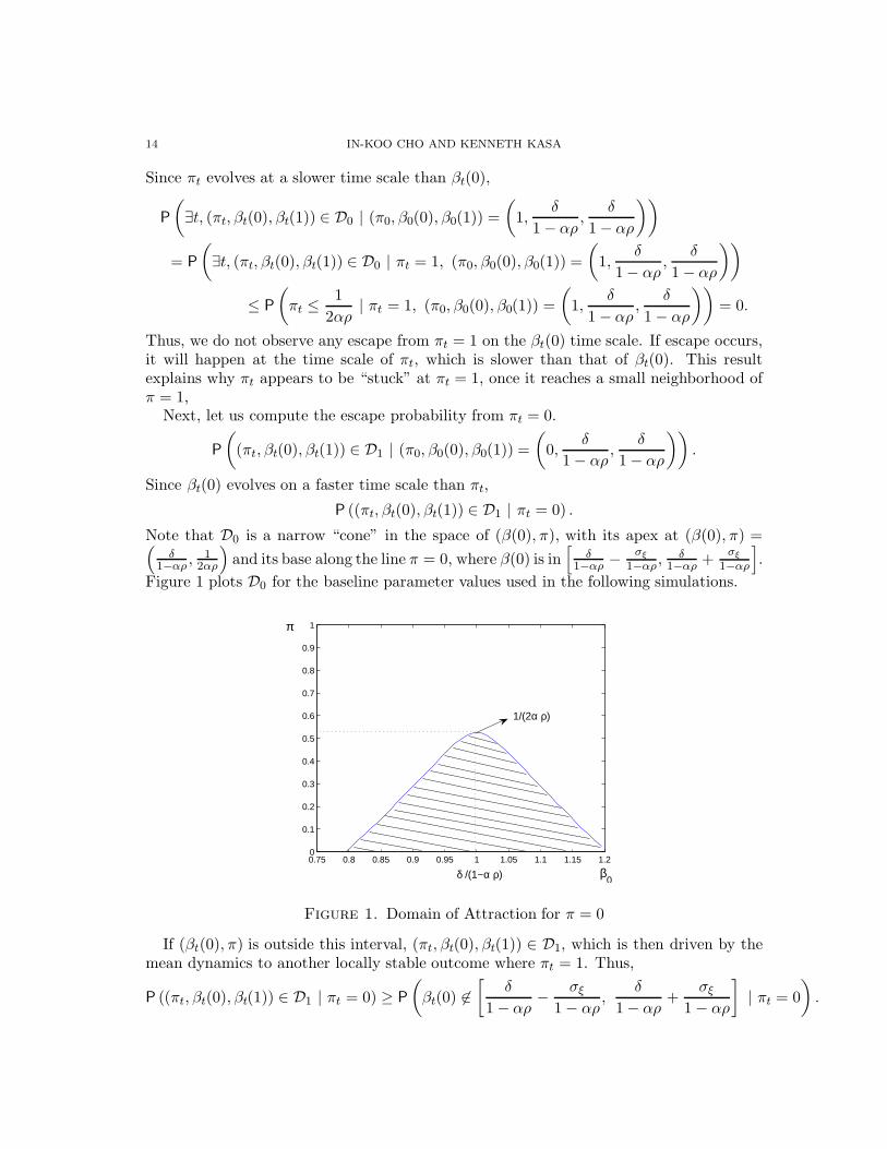
Figure 1 plots D0 for the baseline parameter values used in the following simulations.

0.75 0.8 0.85 0.9 0.95 1 1.05 1.1 1.15 1.20

0.1

0.2

0.3

0.4

0.5

0.6

0.7

0.8

0.9

1π

1/(2α ρ)

δ /(1−α ρ) β0

Figure 1. Domain of Attraction for π = 0

If (βt(0), π) is outside this interval, (πt, βt(0), βt(1)) ∈ D1, which is then driven by themean dynamics to another locally stable outcome where πt = 1. Thus,

P ((πt, βt(0), βt(1)) ∈ D1 | πt = 0) ≥ P

(βt(0) 6∈

[δ

1 − αρ− σξ

1 − αρ,

δ

1 − αρ+

σξ

1 − αρ

]| πt = 0

).


Since βt(0) evolves according to (2.6), which satisfies the regularity conditions in Dupuisand Kushner (1989), we know that βt(0) has a finite but strictly positive large deviationsrate function, which means that the right hand side is of order e−tr∗ , where 0 < r∗ < ∞.Therefore,

limσ2

v→0limt→∞

P((πt, βt(0), βt(1)) ∈ D0 | (π0, β0(0), β0(1)) =

(1, δ


))

P((πt, βt(0), βt(1)) ∈ D1 | (π0, β0(0), β0(1)) =

(0, δ


)) = 0

as claimed. ut

This result shows that the TVP model asymptotically dominates. It will be used ‘almostalways’. This is because it is better able to react to the volatility that it itself creates!Although M1 is misspecified and Pareto suboptimal relative to the Rational Expectationsequilibrium, in practice this equilibrium must be learned via some adaptive process, andwhat our result shows is that this learning process can be subverted by the mere presenceof misspecified alternatives, even when the correctly specified model would converge ifconsidered in isolation. This result therefore echoes the conclusions of Sargent (1993), whonotes that adaptive learning models often need a lot of ‘prompting’ before they converge.Elimination of misspecified alternatives can be interpreted as a form of prompting. Ourresult also offers an interesting counterpoint to Kalai and Lehrer (1993). Despite theapparent satisfaction of their ‘grain of truth’ condition (since π0 < 1), Bayesian learningconverges to the ‘wrong’ model. We discuss this apparent contradiction in more detail inSection 5.

One should keep in mind that, like all asymptotic results, the empirical relevance of thisresult is certainly open to question. Although e−tr∗ remains positive for all t, it becomesa very small number, very quickly. This means that M0 can survive for a long time,especially if it has already withstood the test of time. In fact, since the escape probabilityfrom M0 declines rapidly with respect to calendar time, if M1 is going to dominate onany sort of realistic time scale, it must do so relatively quickly. However, we can onlyaddress these finite sample issues via simulations, to which we now turn.

4. Simulations

As noted in Section 2, the present-value asset pricing model in eqs. (2.1)-(2.2) has beensubjected to a lot of previous empirical work, mostly with negative results. Perhaps itsbiggest problem is its failure to generate sufficient volatility (Shiller (1989)). Our resultssuggest that this negative assessment could be premature. To examine this possibility,we calibrate the model using parameter values that have been used in the past, and seewhether this can generate the sort of self-confirming volatility that our analysis suggestsis possible.

Most of the parameters are easy to calibrate. We know observed fundamentals arepersistent, so we set ρ = .99. Remember, the agent is assumed to know this. Similarly, weknow discount factors are close to 1, so we set the feedback parameter to α = .96. Sinceδ depends on units, we just normalize it by setting δ = (1 − αρ). This implies the self-confirming equilibrium value, β = 1.0. In principle, the innovations variances, (σ2, σ2

z),could be calibrated to match those of observed assets prices and fundamentals. However,


since what really matters is the comparison between actual and predicted volatility, wefollow Evans, Honkapohja, Sargent, and Williams (2013) and just normalize them to unity(σ2 = σ2

z = 1). That leaves one remaining free parameter, σ2v . Of course, this is a crucial

parameter, since it determines the agent’s prior beliefs about parameter instability. If it’stoo big, then the TVP model will be at a big disadvantage during tranquil times, andwill therefore have a difficult time displacing the constant parameter model. On the otherhand, if it’s too small, self-confirming volatility will be empirically irrelevant.

Figures 2-5 report typical simulations for three alternative values, σ2v = (.0005, , .0001, .00001).

0 500 1000 1500 2000−20

−10

0

10

20Price

0 500 1000 1500 20000

0.2

0.4

0.6

0.8

1Pi

0 500 1000 1500 2000−0.5

0

0.5

1Beta0

0 500 1000 1500 2000−0.5

0

0.5

1

1.5Beta1

Figure 2. σ2v = .0005

0 500 1000 1500 2000−20

−10

0

10

20Price

0 500 1000 1500 20000

0.2

0.4

0.6

0.8

1Pi

0 500 1000 1500 20000

0.5

1

1.5Beta0

0 500 1000 1500 20000

0.5

1

1.5Beta1

Figure 3. σ2v = .0005

0 500 1000 1500 2000−10

0

10

20

30Price

0 500 1000 1500 20000

0.2

0.4

0.6

0.8

1Pi

0 500 1000 1500 20000.7

0.8

0.9

1

1.1Beta0

0 500 1000 1500 20000.5

1

1.5Beta1

Figure 4. σ2v = .0001

0 1000 2000 3000 4000−40

−20

0

20Price

0 1000 2000 3000 40000

0.2

0.4

0.6

0.8

1Pi

0 1000 2000 3000 40000.9

1

1.1

1.2

1.3Beta0

0 1000 2000 3000 4000

0.8

1

1.2

1.4Beta1

Figure 5. σ2v = .00001

Figures 2-3 are for the value σ2v = .0005. When this is the case, steady-state price

volatility is 93.3% higher when π = 1 than when π = 0, which is quite significant, althoughless than the excess volatility detected by Shiller (1989). The higher price volatility whenπ = 1 is apparent. The implied steady-state gain associated with this value of σ2

v isγ = .07, which is quite typical of values used in prior empirical work. These figures alsoillustrate a typical feature of the sample paths when σ2

v is relatively high, i.e., convergenceto one or the other boundaries occurs relatively quickly, usually by around T = 500.


Figures 4-5 use smaller values of σ2v . Generally speaking, smaller values of σ2

v delayconvergence. In Figure 4, where σ2

v = .0001, convergence to π = 1 once again takes place,but now its price volatility implications are not quite so dramatic. Volatility is only 41.7%higher when π = 1. Once again, the implied steady-state gain (γ = .03) is typical of valuesused in empirical work. Figure 5 uses a still smaller prior variance, σ2

v = .00001. Now thetwo models do not differ by much. Steady-state price volatility is only 13% higher whenπ = 1. Notice that because the two models are so similar, it becomes easier to escape theπ = 1 equilibrium. Since the TVP world is not that volatile, a constant parameter modeldoes not do that badly.10

The one feature that is perhaps not accurately portrayed by these figures is the fact thaton empirically relevant time-scales convergence to either boundary can occur. This fact wasemphasized by Evans, Honkapohja, Sargent, and Williams (2013). Although our previousresults imply that eventually the π = 1 equilibrium will dominate, our simulations indicatethat the π = 0 equilibrium can persist for a long time. For example, we conducted 10,000simulations, each of length T = 2000, and counted the proportion of times convergenceto π = 1 occurred for various values of σ2

v . As above, the simulations were initialized atπ = 0.5, with small random perturbations of the coefficients around their self-confirmingequilibrium values. Figure 6 displays the results,

−1 0 1 2 3 4 5 6 7

x 10−4

0

0.1

0.2

0.3

0.4

0.5

0.6

0.7

0.8

0.9

σ2v

Figure 6. Prob of Convergence to π = 1

Not surprisingly, the probability of convergence to π = 1 declines with σ2v . For σ2

v =.1 × 10−4, convergence occurs more than 80% of the time, whereas for the benchmarkvalue used above, σ2

v = 5 × 10−4, convergence to π = 1 occurs only about 60% of thetime.11 As our above analysis makes clear, however, one must exercise some caution wheninterpreting results like these. In Figure 6, ‘convergence’ was simply defined as the value ofπ at the end of each simulation run (i.e., at T = 2000). According to our large deviationsresults, however, eventually π will escape from 1. What our theory actually predicts isthat as the sample length becomes infinitely long, the proportion of time spent near π = 1goes to unity. It doesn’t imply that π never returns to 0. Although escapes from π = 1are more likely to occur relatively early in the game, before βt(0) has settled down, as

10Notice that Figure 5 uses a T = 4000 sample length, while Figures 2-4 use T = 2000. As σ2v decreases,

things evolve more slowly, so it becomes necessary to expand the simulation length.11For σ2

v = 0 convergence should occur 50% of the time.


σ2v decreases, escapes can occur relatively late as well. Figure 5 nicely illustrates this

possibility. Hence, the results in Figure 6 are merely meant to convey the possibility thaton realistic time-scales, ‘convergence’ to either π = 1 or to π = 0 can occur.

The fact that convergence to either π = 0 or π = 1 can occur on relevant time-scalesis interesting, since it suggests that whether we live in a tranquil or volatile economy issomewhat random and history-dependent. It also highlights a potentially adverse long-term effect of ‘large deviation’ events, like financial crises. Although being alert to thepossibility of financial crises is probably a good thing on net, if it makes individuals livingin a less than fully understood self-referential environment more reactive, it could createits own problems.

5. Discussion

The results thus far cast doubt on the ability of agents to adaptively learn RationalExpectations Equilibria. Here we discuss the robustness of these results. We do so byconsidering two modifications of the model space. The first narrows the domain of M0

by only considering a single constant parameter model, i.e., the rational expectationsequilibrium in eq. (2.3). The second convexifies the model space directly, by allowing theagent to consider any arbitrary value of σ2

v , rather than just convex combinations of twoextreme values, as was done in the previous model averaging exercise.

5.1. Grain of truth? Kalai and Lehrer (1993) showed that Bayesian learning convergesto Nash equilibrium in repeated games as long as players’ priors concerning their rivals’strategies contain a ‘grain of truth’. That is, as long as priors and the induced distributionof play are mutually absolutely continuous. Although here there is only a single agent,and no strategic interaction, Kalai and Lehrer’s (1993) result is still of some interest,since as usual we can interpret model uncertainty as reflecting the unknown choice ofa fictitious player called ‘nature’. From this perspective, the above results may seempuzzling. After all, M0 appears to be correctly specified, since it contains the rationalexpectations equilibrium

β∗ =δ

1− ρα

as an element. However, as was noted in Section 2.2, all constant parameter models aremisspecified during the transition, as they neglect feedback induced parameter variation.It is only in the limit that they become correctly specified. This may seem like a techni-cality, but it is central to our Gresham’s Law result. If the agent only entertains constantparameter models, then learning does indeed converge to the Rational Expectations Equi-librium (assuming the usual E-stability conditions). However, we showed above that if theagent expands the initial model class only slightly, and in a very natural way, to considerTVP alternatives, then the usual convergence and E-stability results evaporate. In a sense,TVP models can exploit the transition dynamics, and eventually drive out the constantparameter model.

Given this result, it is natural to ask the following question - What if we shut down themisspecified transition dynamics by endowing the agent with more a priori knowledge?Suppose he knows that the true model is either the single constant parameter model ineq. (2.3), or a TVP alternative, which he adaptively updates as usual. He then bases his


forecasts on a Bayesian model averaging strategy as before. Narrowing the initial modelspace in this way produces the folowing result,

Proposition 5.1. Suppose that M0 consists of only the rational expectations equilibrium,and assume αρ < 1. For given σ2

v > 0, the Bayesian learning dynamics of πt converge onfinite time intervals to either 1 or 0, but over infinite horizons we have

limσv→0

limt→∞

πt = 0.

Proof. See Appendix D ut

Interestingly, this is precisely the opposite of our Gresham’s Law result! Now Kalai-Lehrer (1993) seems to ‘work’, and the agent eventually learns the true model. To seewhy this happens, refer back to Figure 1, which depicts the basin of attraction for π = 0.Before, when the constant parameter model had to be estimated, escapes to π = 1 couldoccur ‘horizontally’, as estimates of βt(0) fluctuated. Indeed, since we saw that βt(0)evolves much faster than πt in the neighborhood of π = 0, this is in fact the way escapesoccur (at least with very high probability). Now, however, with only a single constantparameter model on the table, escapes to π = 1 must occur ‘vertically’. This is much moredifficult, since πt evolves so slowly. Somewhat ironically, although the size of the basin ofattraction shrinks to just a vertical line at βt(0) = δ/(1− αρ), its durability increases.

Although Proposition 5.1 predicts the asymptotic distribution of πt is degenerate, itdoes make predictions about finite sample distributions as well. The constant parametermodel (π = 0) now dominates because its basin of attraction is now larger. Escapes fromeach model occur along a vertical line determined by the (identical) self-confirming valuesof the coefficients (i.e., β(i) = δ/(1 − αρ)). The threshold value of π determining theboundary between the two basins of attraction is π∗ = 1/(2αρ). Note that π∗ > 1/2 aslong as αρ < 1. Hence, the basin of attraction of M0 is larger, and so it asymptoticallydominates. This result also suggests, however, that the rate at which this occurs dependson the strength of expectational feedback, i.e., on the magnitude of α. As α increases,the boundary of the basin of attraction moves away from π = 1, making it harder toescape from the TVP model. Therefore, on finite time intervals, we should find that theproportion of sample paths that appear to converge to π = 1 increases as α increases.

Figure 7 corroborates this prediction. We conducted 1200 simulations, each of lengthT = 40, 000 periods, for five different values of the feedback parameter, ranging fromα = .56 to α = .96 in increments of 0.1. We set σ2

v = .0001 in all simulations. (All otherparameter values are the same as in the benchmark calibration discussed in the previoussection). Figure 7 reports the proportion of the 1200 simulation runs that end at π = 1when T = 40, 000. Our large deviations analysis suggests that this proportion shouldincrease with α, and that is precisely what we find. Note, however, that the proportion isalways less than 0.5. Remember that in this asset-pricing context, empirically plausiblevalues of α are close to one. So even if the constant parameter model eventually prevails,the TVP model can persist for a long time with reasonably high probability.


0.5 0.6 0.7 0.8 0.9 10

0.05

0.1

0.15

0.2

0.25

0.3

0.35

0.4

0.45

α

Figure 7. Prob of Convergence to π = 1

In our view, Proposition 5.1 should offer little consolation to those wishing to baseRational Expectations Equilibria on adaptive learning foundations, for two reasons: (1)As emphasized by Nachbar (1997) and Young (2004), Bayesian learning only works herebecause the agent’s prior is very informative.12 He must commit himself to ruling out apriori many reasonable alternatives (i.e., any constant parameter model other than themeasure zero Rational Expectations Equilibrium). Where does this knowledge come from?The whole idea behind learning is that if agents are initially open-minded, experience willallow them to discard incorrect beliefs, and to eventually discover ‘the truth’. In contrast,for learning to work here, agents must be initially closed-minded in just the right way.(2) Given the usual adaptive learning convergence results, one might naively suspect thatthe convergence to π = 0 observed in Proposition 5.1 occurs on a Law of Large Numberst−1 time-scale. Unfortunately, this is not the case. Since πt = 1 is locally stable, escapesto πt = 0 occur on an exponentially long large deviations time scale. This time-scale isorders of magnitude longer than the time-scale governing convergence to π = 1 in ourearlier Gresham’s Law result.

5.2. Convexification. . Normally, with exogenous data,

6. Conclusion

Parameter instability is a fact of life for applied econometricians. This paper has pro-posed one explanation for why this might be. We show that if econometric models areused in a less than fully understood self-referential environment, parameter instability canbecome a self-confirming equilibrium. Parameter estimates are unstable simply becausemodel-builders think they might be unstable.

Clearly, this sort of volatility trap is an undesirable state of affairs, which raises questionsabout how it could be avoided. There are two main possibilities. First, not surprisingly,better theory would produce better outcomes. The agents here suffer bad outcomes be-cause they do not fully understand their environment. If they knew the true model ineq. (2.1), they would know that data are endogenous, and would avoid reacting to theirown shadows. They would simply estimate a constant parameters reduced form model. Asecond, and arguably more realistic possibility, is to devise econometric procedures that

12In the language of Sargent (1993), we have provided the agent with a lot of ‘prompting’.


are more robust to misspecified endogeneity. In Cho and Kasa (2015), we argue that inthis sort of environment, model selection might actually be preferable to model averag-ing. Another possibility would be to convexify the model space in a different way. Herethe agent mixes between two discretely different models. Normally, when the data areexogenous, it would make no difference whether a parameter known to lie in some inter-val is estimated by mixing between the two extremes, or by estimating it directly. Withendogenous data, however, this could make a difference. What if the agent convexified byestimating σ2

v directly, via some sort of nonlinear adaptive filtering algorithm (e.g., Mehra(1972)), or perhaps by estimating a time-varying gain instead, via an adaptive step-sizealgorithm (Kushner and Yang (1995))? Although π = 1 is locally stable against nonlocalalternative models, would it also be stable against local alternatives? Intuition suggeststhat as long as the usual sort of ‘E-stability’ conditions are satisfied, this might not be thecase. On the other hand, in practice, models are not continuously revised, and our resultshere suggest that when this is the case, parameter instability and its induced volatilitycan indeed become a trap.


Appendix A. Proof of Proposition 2.2

For any σv > 0, we know from our analysis in sections 2.2 and 2.3 that βt(1) evolves ‘faster’ than βt(0).We want to exploit this time-scale separation when deriving asymptotic approximations. To do this, weassume σv → 0 more slowly than t−1 → 0, so that t ·σv → ∞. In other words, we assume σv = O(t−(1−δ))for some δ > 0. Given this, we can derive the following mean ODE for β(0) and the following diffusion forβ(1) (we do not provide the details here, since they are standard. See, e.g., Evans and Honkapohja (2001))

β̇(0) = δ + αρ[πβ(1) + (1 − π)β(0)] − β(0) (A.17)

dβ(1) = −(1 − αρπ)[β(1)− β̄(1)]dt + σvdW (A.18)

where

β̄(1) =δ + αρ(1 − π)β(0)

1 − αρπ(A.19)

is the long-run mean of β(1). Note that it depends on β(0). Also note that this system is globally stable

as long as αρ < 1. Now, since σv = O(t−(1−δ)), we can assume that β(1) has converged to its long-runmean for any given value β(0). Therefore, we can simply substitute the long-run mean in eq. (A.19) into(A.17) to derive the following autonomous ODE for β(0)

β̇(0) = (1 − αρπ)−1[δ − (1 − αρ)β(0)] (A.20)

Note that this converges to δ/(1−αρ) for all π ∈ (0, 1). Finally, if substitute β(0) = δ/(1−αρ) into (A.19)we find β(1) = δ/(1 − αρ) also, again for all π ∈ (0, 1). �

Appendix B. Proof of Lemma 3.2

Fix a sequence {πt} in Π0. Since the sequence is a subset of a compact set, it has a convergentsubsequence. After renumbering the subsequence, let us assume that

limt→∞

πt = π∗ ∈ (0, 1)

since {πt} ∈ Π0. Depending upon the rate of convergence (or the time scale according to which πt convergesto π∗), we have to treat πt has already converged to π∗.13

We only prove the case in which πt → π∗ according to the fastest time scale, in particular, faster thanthe time scale of βt(1). Proofs for the remaining cases follow the same logic.

Since πt evolves according to the fastest time scale, assume that

πt = π∗.

Under the assumption of Gaussian distributions,

lnAt(0)

At(1)= − (pt − ρβt(0)zt)

2

2(σ2 + Σt(0)z2t )

+(pt − ρβt(1)zt)

2

2(σ2 + Σt(1)z2t )

+1

2ln

[σ2 + Σt(1)z

2t

σ2 + Σt(0)z2t

]. (B.21)

Since the first two terms are normalized Gaussian variables,

E lnAt(0)

At(1)= E

1

2ln

[σ2 + Σt(1)z

2t

σ2 + Σt(0)z2t

].

Recall (2.6), and note that Σt(0) → 0. On the other hand, Σt(1) is uniformly bounded away from 0, ast → ∞, and the lower bound converges to 0, as σ2

v → 0. Thus, βt(1) evolves on a faster time scale thanβt(0). In calculating the limit value of (B.21), we first let βt(1) reach its own “limit”, and then let βt(0)go to its own limit point.

Let pet (i) be the period-t price forecast by model i,

pet (1) = ρβt(1)zt.

Since

pt = αρ[(1− πt)βt(0) + πtβt(1)]zt + δzt + σεt,

13If πt evolves at a slower time scale than βt(0), then we fix πt while investigating the asymptotic propertiesof βt(0). As it turns out, we obtain the same conclusion for all cases.


the forecast error of model 1 is

pt − pet (1) = [αρ(1 − πt)βt(0) + (αρπt − 1)βt(1) + δ] zt + σεt.

Since βt(1) evolves according to (2.6),

limt→∞

E [αρ(1 − πt)βt(0) + (αρπt − 1)βt(1) + δ] = 0

in any limit point of the Bayesian learning dynamics.14 Since βt(1) evolves at a faster rate than βt(0), wecan treat βt(0) as a constant. Since πt = πs, we treat πt as constant also.15 Define

β(1) = limt→0

Eβt(1)

whose value is conditioned on πt and βt(0). Since

limΣt(1)

limt→0

[αρ(1 − πt)βt(0) + (αρπt − 1)β(1) + δ

]+ E(αρπt − 1)(βt(1) − β(1)) = 0.

Thus, as we found in the proof of Proposition 2.2,

β(1) = Eαρ(1 − πt)βt(0) + δ

1 − αρπt.

Define the deviation from the long-run mean as

ξt = βt(1) − β(1).

Model 1’s mean-squared forecast error is then

limt→0

E(pt − pet (1))

2 = limt→0

Ez2t (αρπt − 1)2σ2

ξ + σ2

Note that

limσ2

v→0σ2

ξ = 0.

To investigate the asymptotic properties of βt(0), let us write

βt(1) =αρ(1 − πt)βt(0) + δ

1 − αρπt+ ξt

Then, we can write Model 0’s forecast error as

pt − pet (0) = zt

[− 1 − αρ

1 − αρπt

(βt(0) −

δ

1 − αρ

)+ αρπtξt

]+ σεt.

Since βt(0) evolves according to (2.6)

limt→∞

βt(0) =δ

1 − αρ

with probability 1. Thus, the mean-squared forecast error satisfies

limt→∞

E(pt − pet (0))

2 = limt→∞

Ez2t σ2

ξ(αρπt)2 + σ2

Thus, once again as in the proof of Propostion 2.2, in the long run

limt→0

βt(1) =δ

1 − αρ

in distribution, as Σt(1) → 0 or equivalently, σ2v → 0. Note that

limt→∞

E(pt − pet (0))

2

E(pt − pet (1))

2> 1 (B.22)

if and only if

limt→∞

(αρπt

1 − αρπt

)2

> 1.

14Existence is implied by the tightness of the underlying space.15If πt evolves on a slower time scale than βt(1), we treat πt as a constant, while investigating the asymptoticproperties of βt(1).


Now, notice thatαρπt

1 − αρπt< 1

if and only if

αρπt <1

2.

Hence, if (B.22) holds for some t ≥ 1, then it holds again for t + 1, and vice versa. Thus, πt continues toincrease or decrease, if the inequality holds in either direction. Recall that π∗ = limt→∞ πt. Convergenceto π∗ can occur only if (B.22) holds with equality for all t ≥ 1, which is a zero probability event. Weconclude that π∗ ∈ (0, 1) occurs with probability 0. �

Appendix C. Proof of Lemma 3.3

A simple calculation shows

t(πt − πt−1) =t(e(t−1)φt−1 − etφt)

(1 + etφt)(1 + e(t−1)φt−1 ).

As t → ∞, we know φt → φ∗ with probability 1. We also know t(φt − φt−1) is uniformly bounded. Hence,we have

limt→∞

t(πt − πt−1) = limt→∞

t(e−φ∗

− 1)

etφ∗

(1 + etφ∗ )(1 + e(t−1)φ∗)

= (e−φ∗− 1) lim

t→∞

t

(1 + e−tφ∗ )(1 + etφ∗e−φ∗ )

Finally, notice that for both φ∗ > 0 and φ∗ < 0 the denominator converges to ∞ faster than thenumerator. �

Appendix D. Proof of Proposition 5.1

Recall that

φt =1

t

t∑

k=1

logAk(0)

Ak(1)

where βt(0) is updated according to (2.6). Now let us fix βt(0) = β∗, and define the corresponding valueof φt as φe

t . Note that since βt(0) → β∗,

φ∗ = E logAt(0)

At(1)

is defined for βt(0) = β∗. Following the same logic as in the text,

φet = φe

t−1 +1

t(φ∗ − φe

t−1)

andφe

t → φ∗

with probability 1, as t → ∞.One can easily verify that φ∗ < 0 only if limt→∞ πt = 1, and φ∗ > 0 only if limt→∞ πt = 0. To

differentiate the two locally stable points of φet , let us write φ∗

+ > 0 and φ∗− < 0 for the positive and

negative locally stable points of φet . Note that the domain of attraction for φ∗

− is D1, and similarly, thedomain of attraction for φ∗

+ is D0. A simple calculation shows that

φ∗+ + φ∗

− > 0.

That is, φ∗+ is further away from the boundary of its domain of attraction than φ∗

−.We need to calculate

limt→∞

P(∃t, (πt, βt(0), βt(1)) ∈ D0 | (π0, β0(0), β0(1)) =

(1, δ

1−αρ, δ

1−αρ

))

P(∃t, (πt, βt(0), βt(1)) ∈ D1 | (π0, β0(0), β0(1)) =

(0, δ

1−αρ, δ

1−αρ

)) . (D.23)


If the limit vanishes,the transition from D0 to D1 dominates the transition from D1 to D0, which impliesthat as σ2

v → 0, the probability is massed at the stable point in D1, i.e., π = 1. On the other hand, if thelimit explodes, then the probability mass of πt converges to 1 at πt = 0.

Note

P

(∃t, (πt, βt(0), βt(1)) ∈ D0 | (π0, β0(0), β0(1)) =

(1,

δ

1 − αρ,

δ

1 − αρ

))

= P (∃t, φet > 0 | φe

0 = φ∗ < 0)

and

P

(∃t, (πt, βt(0), βt(1)) ∈ D1 | (π0, β0(0), β0(1)) =

(0,

δ

1 − αρ,

δ

1 − αρ

))

= P (∃t, φet < 0 | φe

0 = φ∗ > 0) .

The right hand side of both equations can be approximated as

limt→∞

−1

tlog P (∃t, φe

t < 0 | φe0 = φ∗

+ > 0) = r∗0

and

limt→∞

−1

tlog P (∃t, φe

t > 0 | φe0 = φ∗

− < 0) = r∗1 ,

where r∗0 and r∗1 are the values of the potential function of ODE at the boundary of the domain of theattraction (i.e., φe = 0). Note that (D.23) explodes if r∗0 > r∗1 , from which the conclusion of the propositionfollows.

Since the dynamics of φet is approximated by a one-dimensional ODE

φ̇e = φ∗ − φe,

the potential function exists. Following Example 3.1 on page 121 of Freidlin and Wentzell (1998), we knowthat the potential function is

U(τ) = −∫ τ

0

E log φ∗ − φe(s)ds

where τ is the first exit time from the domain of the attraction with φe(0) = φ∗. Let us write U(τ)∣∣φ∗+>0

and U(τ)∣∣φ∗−<0

for the potential function around the neighborhood of π = 0 and π = 1, respectively. We

apply the same convention to other variables.Since we assume that ρα < 1, one can easily show that

φ∗+ + φ∗

− > 0.

Thus,r∗0 = U(τ)

∣∣φ∗+>0

> U(τ)∣∣φ∗+<0

= r∗1 > 0,

as desired. �


References

Bacchetta, P., and E. van Wincoop (2013): “On the Unstable Relationship Between Exchange Ratesand Macroeconomic Fundamentals,” Journal of International Economics, 91, 18–26.

Benhabib, J., and C. Dave (2014): “Learning, Large Deviations and Rare Events,” Review of EconomicDynamics, 17, 367–382.

Benveniste, A., M. Metivier, and P. Priouret (1990): Adaptive Algorithms and Stochastic Approx-imations. Springer-Verlag, Berlin.

Borkar, V. S. (2008): Stochastic Approximation: A Dynamical Systems Viewpoint. Cambridge UniversityPress.

Bray, M., and N. Savin (1986): “Rational Expectatons Equilibria, Learning, and Model Specification,”Econometrica, 54, 1129–60.

Bullard, J. (1992): “Time-Varying Parameters and Nonconvergence to Rational Expectations underLeast-Squares Learning,” Economics Letters, 40, 159–66.

Chakraborty, A., and G. W. Evans (2008): “Can Perpetual Learning Explain the Forward PremiumPuzzle?,” Journal of Monetary Economics, 55, 477–90.

Cho, I.-K., and K. Kasa (2015): “Learning and Model Validation,” Review of Economic Studies, 82,45–82.

Cho, I.-K., N. Williams, and T. J. Sargent (2002): “Escaping Nash Inflation,” Review of EconomicStudies, 69, 1–40.

Cogley, T., and T. J. Sargent (2005): “Drift and Volatilities: Monetary Policies and Outcomes in thepost WWII US,” Review of Economic Dynamics, 8, 262–302.

DeRoover, R. (1949): Gresham: On Foreign Exchange. Harvard University Press.Dupuis, P., and H. J. Kushner (1989): “Stochastic Approximation and Large Deviations: Upper Boundsand w.p.1 Convergence,” SIAM Journal of Control and Optimization, 27, 1108–1135.

Esponda, I., and D. Pouzo (2014): “An Equilibrium Framework for Players with Misspecified Models,”University of Washington and University of California, Berkeley.

Evans, G. W., and S. Honkapohja (1993): “Adaptive Forecasts, Hysteresis and Endogenous Fluctua-tions,” Economic Review of Federal Reserve Bank of San Francisco, 1, 3–13.

(2001): Learning and Expectations in Macroeconomics. Princeton University Press.Evans, G. W., S. Honkapohja, T. J. Sargent, and N. Williams (2013): “Bayesian Model Averaging,Learning, and Model Selection,” in Macroeconomics at the Service of Public Policy, ed. by T. J. Sargent,and J. Vilmunen. Oxford University Press.

Evans, G. W., and G. Ramey (2006): “Adaptive Expectations, Underparameterization, and the LucasCritique,” Journal of Monetary Economics, 53, 249–64.

Fernandez-Villaverde, J., and J. Rubio-Ramirez (2007): “How Structural are Structural Parame-ters?,” in NBER Macroeconomics Annual. MIT Press.

Freidlin, M. I., and A. D. Wentzell (1998): Random Perturbations of Dynamical Systems. Springer-Verlag, second edn.

Hansen, L. P., and T. J. Sargent (2008): Robustness. Princeton University Press.Inoue, A., and B. Rossi (2011): “Identifying the Sources of Instabilities in Macroeconomic Fluctuations,”The Review of Economics and Statistics, 93, 1186–1204.

Kalai, E., and E. Lehrer (1993): “Rational Learning Leads to Nash Equilibrium,” Econometrica, 61,1019–1045.

Kasa, K. (2004): “Learning, Large Deviations, and Recurrent Currency Crises,” International EconomicReview, 45, 141–173.

Kostyshyna, O. (2012): “Application of an Adaptive Step-Size Algorithm in Models of Hyperinflation,”Macroeconomic Dynamics, 16, 355–75.

Kushner, H. J., and J. Yang (1995): “Analysis of Adaptive Step-Size SA Algorithms for ParameterTracking,” IEEE Transactions on Automatic Control, 40, 1403–10.

Lucas, Jr., R. E. (1976): “Econometric Policy Evaluation: A Critique,” in The Phillips Curve and LaborMarkets, ed. by K. Brunner, and A. Meltzer. Carnegie-Rochester Conf. Series on Public Policy.


Marcet, A., and J. P. Nicolini (2003): “Recurrent Hyperinflations and Learning,” American EconomicReview, 93, 1476–98.

McGough, B. (2003): “Statistical Learning with Time-Varying Parameters,” Macroeconomic Dynamics,7, 119–39.

Mehra, R. K. (1972): “Approaches to Adaptive Filtering,” IEEE Transactions of Automatic Control, 17,693–98.

Nachbar, J. H. (1997): “Prediction, Optimization, and Learning in Repeated Games,” Econometrica,65, 275–309.

Rolnick, A. J., and W. E. Weber (1986): “Gresham’s Law or Gresham’s Fallacy?,” Journal of PoliticalEconomy, 94, 185–89.

Sargent, T. J. (1993): Bounded Rationality in Macroeconomics. Clarendon Press.(1999): The Conquest of American Inflation. Princeton University Press.(2008): “Evolution and Intelligent Design,” American Economic Review, 98, 5–37.

Sargent, T. J., and N. Williams (2005): “Impacts of Priors on Convergence and Escapes from NashInflation,” Review of Economic Dynamics, 8, 360–91.

Shiller, R. J. (1989): Market Volatility. MIT Press.Timmermann, A. G. (1996): “Excessive Volatility and Predictability of Stock Prices in AutoregressiveDividend Models with Learning,” Review of Economic Studies, 63, 523–57.

Young, H. P. (2004): Strategic Learning and its Limits. Oxford University Press.

gresham’s law of model averaging - the … · gresham’s law of model averaging in-koo cho and...

Documents