Gregory Ruchti

Senior Thesis

University of Maryland

I. Introduction

Today, electromagnetic simulations have become very useful in creating and

analyzing microwave structures. Now, if one wants to test a certain hypothesis about a

structure, he or she can first use a simulation to see if the hypothesis is at all possible.

Also, simulations can be compared to raw measurements for accuracy and understanding

of a problem. I used two programs to run my electromagnetic simulations: Ansoft High

Frequency Structure Simulator (HFSS) and Ansoft Optimetrics.

Ansoft HFSS is a software package used to simulate the electromagnetic behavior

of a three-dimensional structure. One can easily compute such things as: electromagnetic

field quantities, radiated fields, characteristic port impedances, S-parameters,

eigenmodes, and many other useful quantities. However, for HFSS to compute these

quantities and fields, many conditions must be specified. First, one must draw the

structure and specify the characteristic materials for each object. Next, the sources, ports,

and special surface boundary conditions must be identified. Once all this has been

specified, HFSS will compute a solution to Maxwell’s equations with all the necessary

fields.

Ansoft Optimetrics is very similar to HFSS, however, it has a “batching” program

that is very useful. Optimetrics takes an HFSS-defined model and can perform

optimization and parametric analyses of the model. What is even better is that it allows

1

the user to simulate design variations using a single, or “nominal”, model! You no longer

need to create a new model to calculate for each new variation. Ansoft Optimetrics will

do that all in one project. Also, one can define a cost function, which the optimizer

function of Optimetrics will attempt to find a minimum value. This function is very

useful, and example of this is illustrated in Chapter 2.

These two simulators have become very useful tools in designing and analyzing

microwave and electromagnetic structures. Below I will illustrate five projects that were

completed using one or both of these programs. Also, I have included a technical notes

section in Appendix C, which give some helpful facts about the programs.

2

II. Ansoft HFSS and Optimetrics Projects

1. Radiation from Open-Ended Coaxial Probes

In order to understand the power radiated from an open-ended coaxial probe with center

conductor extended as an STM tip such as Atif Imtiaz’s microscope, I created simplified

versions of the typical MWM/STM experiment, which included only a coaxial cable

without a tip in an empty radiation box. No sample was present. An analytical solution

is known for the case of an open coaxial probe with an infinite ground plane extension,

radiating into free space [1].

Figure 1. Typical setup for the open-ended coaxial probe and radiation box. The dimensions included are that of the largest radiation box I used.

I varied the size of the radiation box, which produced variations in the radiated power.

The pattern these variations produced is shown in Figures 2 and 3.

3

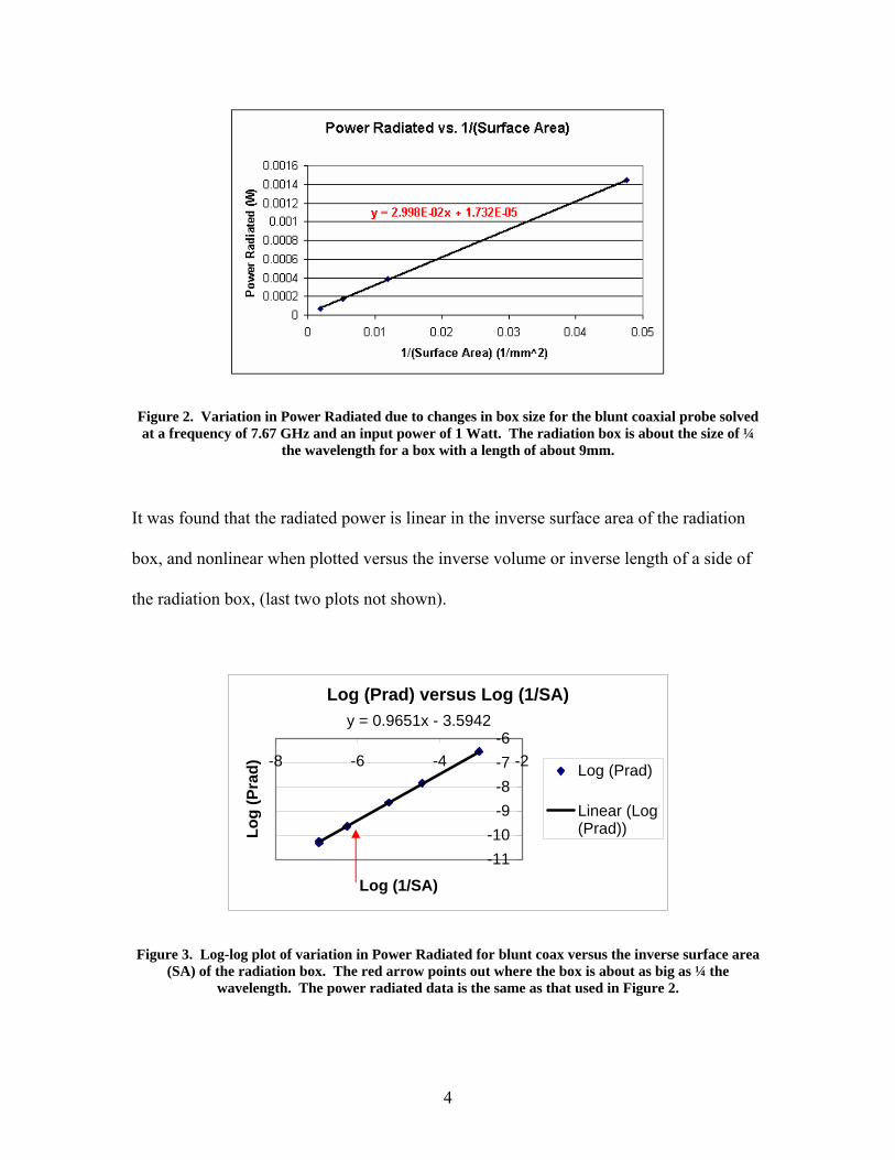
Figure 2. Variation in Power Radiated due to changes in box size for the blunt coaxial probe solved at a frequency of 7.67 GHz and an input power of 1 Watt. The radiation box is about the size of ¼

the wavelength for a box with a length of about 9mm.

It was found that the radiated power is linear in the inverse surface area of the radiation

box, and nonlinear when plotted versus the inverse volume or inverse length of a side of

the radiation box, (last two plots not shown).

Log (Prad) versus Log (1/SA)y = 0.9651x - 3.5942

-11-10

-9-8-7-6

-8 -6 -4 -2

Log (1/SA)

Log

(Pra

d) Log (Prad)

Linear (Log(Prad))

Figure 3. Log-log plot of variation in Power Radiated for blunt coax versus the inverse surface area (SA) of the radiation box. The red arrow points out where the box is about as big as ¼ the

wavelength. The power radiated data is the same as that used in Figure 2.

4

From these graphs, it can be deduced that as the radiation box gets larger, the power

radiated gets smaller.

The HFSS manual claims that the radiation box should be bigger than a fourth of

the wavelength, meaning the sides of the box should be a fourth of a wavelength or

farther from the objects inside. This is consistent with my data. Furthermore, the

analytical value for the power radiated for a blunt coax with an infinite ground plane,

similar to the one I created for these experiments can be found using the following

equation, [1]:

( )( )

2

2

22222

ln34

⎟⎟⎠

⎞⎜⎜⎝

⎛ −=

ab

freerad c

fabZVP ππ , (1)

where 0

0

εμ

=freeZ is the impedance of free space, which is about 377 Ohms. V is the

voltage between the inner and outer conductors, found to be 20 Volts from HFSS data.

The inner and outer radii are given as = 0.255 mm and b = 0.84 mm, respectively. The

parameter is the frequency given as 7.67 GHz and c is the speed of light in a vacuum.

After plugging in the necessary values for these parameters, I found a power radiated of

about 5.35E-05 Watts. The intercept from Figure 2 gives a power radiated of 1.73E-05

Watts in the limit of infinite radiation box size. These two values are fairly close, but not

quite the same. Perhaps our linear extrapolation to infinite box size is not valid. Yet,

besides the difference in these values, it is clear that the bigger the radiation box (greater

than or equal to one fourth of the wavelength), the lower the value for the radiated power.

a

f

5

Radiation Loss Results

I created two new models, which were derived from the simplified versions

above. These two models contain an almost identical representation of Atif’s coaxial

cable and STM tip. The difference between the two models is that one has a perfectly

conducting sample 22 nanometers from the tip while the other model contains no sample.

I chose this 22 nm gap because of Aspect Ratio issues (discussed in Appendix Technical

Notes). Also, I made the radiation box very large, (about 3 times a quarter of the

wavelength), in accordance with the results above. A picture of the model, which

contains the perfectly conducting sample is shown in Figure 4.

Driving Port

0.0854" OD

Figure 4. Picture of model with perfect conducting sample. The radiation box, although not completely shown in this picture is 21x21x2.500022 mm.

For the model containing the perfectly conducting sample, I calculated the

radiated power at the radiation boundary so as to determine the radiation Q, , for the

microscope using the following equation:

radQ

radrad P

fUQ π2= , (2)

6

where is the power radiated, is the frequency given as 7.67 GHz, and U is the

energy stored in the entire resonator (not modeled in HFSS), which is estimated to be

2.1E-9 Joules, [2].

radP f

If is much larger than the measured unloaded Q of the resonator then the

power radiated is negligible and can be ignored in further studies with the STM-tipped

microscope. If is small, then the power radiated will be a factor. Results for the

model containing no sample gave a power radiated of 3.309E-3 Watts. Using this along

with the other parameters gave a value for of 30,584, which is very large compared

to , which is about 400. The calculated results of the model containing the

perfectly conducting sample gave as 1.262E-2 Watts. Plugging this into the

equation above gave a of 8019, which again is very large compared to .

From these two models and calculations I determined that was large enough to

safely assume that the power radiated is negligible for Q measurements in STM tipped

microwave microscope studies.

radQ

radQ

radQ

unloadedQ

radP

radQ unloadedQ

radQ

Conclusions

When I develop new models in the future, to gain accurate results on the power

radiated, I must create radiation boxes that are very large and comparable in size to a

fourth of the size of the wavelength of a microwave signal. However, as was determined

above, it is safe to assume that any power radiated is negligible compared to other losses.

Model Power Radiated Q radiated

Blunt coax/ no sample 1.73E-5 Watts 5.8 x 106

Stm-tip/ no sample 3.3E-3 Watts 30584

Stm-tip/ with sample 1.26E-2 Watts 8019

7

Indeed, the power radiated can be ignored in further studies with the microwave

microscopes, until the of the microscope increases into the 10unloadedQ 3 range.

REFERENCES

[1] Everette C. Burdette, F. L. Cain, and J. Seals. "In Vivo Probe Measurement

Technique for Determining Dielectric Properties at VHF Through Microwave

Frequencies." IEEE Transactions On Microwave Theory and Techniques. Pg.

414. Vol. MTT-28, No. 4. April 1980.

[2] Atif NFSMM Model, Notebook 344. Pages 48-49.

8

3. Loop Probe Model

Theory

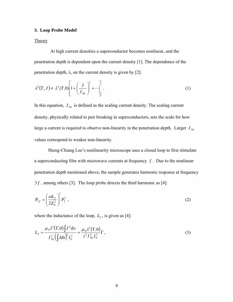
At high current densities a superconductor becomes nonlinear, and the

penetration depth is dependent upon the current density [1]. The dependence of the

penetration depth, λ, on the current density is given by [2]:

( )⎥⎥⎦

⎤

⎢⎢⎣

⎡+⎟⎟

⎠

⎞⎜⎜⎝

⎛+∝ L

222 1)0,(,

NLJJTJT λλ . (1)

In this equation, is defined as the scaling current density. The scaling current

density, physically related to pair breaking in superconductors, sets the scale for how

large a current is required to observe non-linearity in the penetration depth. Larger

values correspond to weaker non-linearity.

NLJ

NLJ

Sheng-Chiang Lee’s nonlinearity microscope uses a closed loop to first stimulate

a superconducting film with microwave currents at frequency . Due to the nonlinear

penetration depth mentioned above, the sample generates harmonic response at frequency

, among others [3]. The loop probe detects the third harmonic as [4]:

f

f3

32

20

23 2 ff P

ZL

P ⎟⎟⎠

⎞⎜⎜⎝

⎛=

ω , (2)

where the inductance of the loop, , is given as [4]: 2L

( )( )

( )Γ==

∫∫

30

23

20

20

22

420

20,0,

IJtT

IJdsJ

dJTL

NLNL

λμυλμ, (3)

9

where t is the superconducting film thickness, ∫= JdsI 0 is the total current,

and∫

∫=Γ

l

dxK

dxdyK

y

S

4

is the geometrical factor serving as the figure of merit for Lee’s

microscope probe.

Now we can easily determine from the measured values of and the calculated

quantities of the figure of merit Γ using the following equation [4]:

2NLJ fP3

( )Γ=

fNL PZt

TJ

303

202

240,ωλμ . (4)

The main purpose of my loop probe models was to find Γ for different loop probe

sizes. The figure of merit could then be used to estimate the sensitivity of the microwave

microscope to non-linearity in the penetration depth, λ. For Lee’s microwave

microscope, Γ is proportional to (max). This means that a large Γ correspond to

better sensitivity to the weaker non-linearity for a given penetration depth, film thickness,

and measured 3

2NLJ

rd harmonic power, which is exactly what Lee wants.

In the above equation, one can see that there is time-reversal symmetry in the

term, because it is squared. John has guessed that there might be an additional term

within the equation for λ, which addresses broken time-reversal symmetry. This new

equation would look like the following:

NLJ

( ) ( )⎥⎥⎦

⎤

⎢⎢⎣

⎡+⎟⎟

⎠

⎞⎜⎜⎝

⎛+

′+∝ L

222 10,,

NLNL JJ

JJTJT λλ . (5)

10

The time-reversal symmetry is broken within the NLJJ′

term. I will also solve for another

quantity, Γ , which is a figure of merit proportional to ′ NLJ ′ (max). The calculation

for using Γ and the second harmonic, , is analogous to the calculation of

using Γ and above.

NLJ ′ ′ fP2 NLJ

fP3

Now, the final question is, how does one find Γ and Γ′ ? The answer lies within

the surface current on the superconductor K, as can be seen in the above equations. Once

I have solved the loop probe models, HFSS will store all fields. By employing Ansoft

HFSS’s Calculator function, I could easily calculate the two figures of merit by using the

following equations [4]:

∫

∫=Γ

l

dxK

dxdyK

y

S

4

and ∫

∫=Γ′

l

dxK

dxdyK

y

S

3

, (6)

where K is the surface current density on the perfectly conducting plane and is the y-

component of the surface current density. One can see that the numerators are surface

integrals, while the denominators are line integrals. The line integrals represent the total

current on the superconductor. These integral equations help make a connection between

different geometries and or

yK

NLJ NLJ ′ .

Setup and Analysis

The loop probe model consists of a coaxial cable, in which the inner conductor curves

around to touch the outer conductor, (as shown in the Figure 12). The bottom of the loop

is 12.5 microns above a perfectly conducting infinite plane. I will also be referring to two

radii: the inner conductor radius, R, and the loop radius, r. Each consecutive model

11

consisted of smaller r and R, and also contained smaller coaxial cables, (given in table

below).

Loop Model Name

Loop Radius r (μm)

Wire Radius R (μm)

Coaxial Cable Diameter (μm)

085 665 250 2160 037 270 100 880 020 172.5 65 560 010 86.25 32.5 280 005 43.125 16.25 140

Figure 5. This is the setup for Loop Probe models. The green line represents the perfect conducting plane. Radiation Box Surrounds entire model.

All of the models were solved at a frequency of 6.5 GHz, and contained a tetrahedron

count of over 100,000 (for mesh resolution quality). Also, to speed up the solution time I

used symmetry in the model to cut it in half, (see Appendix C). The cut-plane I defined

as H-symmetry. (See Figure 18 for picture showing H-symmetry boundary.)

After solving a loop probe model, I took a look at plots of the surface current on

the perfect conducting plane. I noticed a peculiar circular motion in the plots. This

circulating motion is shown in the figure below.

12

Figure 6. This is a plot of the surface current on the perfect conducting plane. There is a very noticeable circular motion in the current. The entire perfectly conducting surface is used for the K4 integral.

Because the current circulates, the line for which my line integrals would be solved had

to be adjusted. One can see that there is a “hole” around which the current circles. The

line that I will integrate over should only extend as far as that hole to get a proper value

for the integrals. The hole’s position changed with the sizes of the loop probes, (see

Figure 14). Therefore, I had to adjust the integration line for each new model.

Figure 7. This is a plot of the "hole" distance versus the loop radius, r, both in mm.

13

Once I had my integration line set, I used the Calculator to solve for Γ and Γ′ . I

then plotted Γ against the loop radius, r, which is shown below.

Figure 8. The Figure of Merit gets very large as the loop size gets very small.

Figure 15 shows that as the loop size gets very small Γ becomes very large. The plot,

however, for is not quite as clear. As shown in Figure 16, the values for follow a

similar pattern. Yet, there is a small hump in the middle of the graph. It is unclear why

that is there.

Γ′ Γ′

Figure 9. There is a peculiar hump in the middle of the graph.

14

I further studied Γ and Γ′ for a very small loop probe. Actually, the loop was so

small that the only feasible way to make it was to put it on what I like to call, the “home

plate”. Below is a picture of the loop probe.

Figure 10. The is a picture of the very small loop, 10 micron radius on sapphire plate.

The loop, which extends from the coaxial cable is now a one micron thick film

which ends in a loop of radius 10 microns and extends back up to the outer conductor.

The film was placed on a 0.5 mm thick sapphire plate, as shown in Figure 17.

The resultant figures of merit agree very well with the plots above. For this

model, Γ = 1.28E+006 A3/m2 and Γ′= 410.212 A2/m. These values are huge compared

to the other loop probes. This shows that very small loop probes will have the highest

sensitivity to the weak nonlinearity.

I moved on to a new type of model, in which I placed a loop probe above a film of

finite, non-zero sheet-resistance atop a substrate. Lee and I wanted to see how a normal

metal thin film, instead of a perfect conductor, would change the values of Γ and .

The new model, which is shown in the figure,

Γ′

15

Figure 11. New model to see how the figures of merit change due to sheet-resistant film. This figure shows the H-symmetry plane used to cut all models in half to speed up solution process.

consisted of a 037 Coaxial Cable loop probe with r equal to 270 μm and R equal to 100

μm. The bottom of the loop was 12.5 μm above a film of sheet-resistance 75 Ω/ . This

film rests on top of a one-millimeter thick LaO substrate, (ε = 24), whose bottom surface

is defined as copper.

Again, using the surface current on the sheet-resistant film, I found Γ and Γ . ′

Figure of Merit Perfect Conductor Sheet Resistance Film

75 Ω/ٱ

Γ 31220 106.379

Γ′ 3.84 0.3

They were noticeably smaller, (by a few orders of magnitude!!), than those values found

on the perfect conducting plane. This in some sense means that Lee’s microscope is

much less sensitive to nonlinearity in a normal metal film compared to a superconducting

film.

Mutual Inductance

16

Another aspect of the loop probe that I analyzed was the mutual inductance

between two “mirrored” loops. Below is the model for this calculation.

Figure 12. Setup for mutual inductance calculations.

The two probes are exactly identical in dimensions and materials. The ends of the loops

are 25 μm from each other. The signal is sent into the top probe via port 1 and is picked

up by the bottom probe at port 2.

The purpose of this calculation is to find the mutual inductance of Lee’s

microscope to determine how much signal is coupled from the sample. The mutual

inductance is given by:

1

2

VVLM = , (6)

where V1 and V2 are the voltage drops between the inner and outer conductors of the

coaxial cables of the top and bottom probes, respectively, (as shown in Figure 19). The

inductance of the bottom loop is given by

17

IL Φ= , (7)

where is the flux through the bottom loop and ∫ •=ΦS

adB rr∫ ∫ •×=•=S C

ldnKadJIrrrr

)ˆ( is

the induced current through the bottom loop. The surface and loop used for solving the

above integrals are shown in Figure 19.

All of the above equations can be easily solved by HFSS, using the Calculator.

However, I ran into somewhat of a problem. The voltages and induced current values

that I calculated depended on what lines and loop, respectively, that I used. Therefore, I

found a range of values for the mutual inductance. The range of values for the mutual

inductance of three different loop sizes is shown in the table below.

Loop Probe Mutual Inductance (H) M/L

085 1.3E-011 to 2.7E-011 0.028 to 0.037

037 1.7E-011 to 2.0E-011 0.03125 to 0.0367

020 2.6E-012 to 2.1E-011 0.026 to 0.038

Essentially, my results show that only about 3% of the signal sent is being coupled from

the sample. This means that this reflected signal must be amplified. This is discussed

more in the next chapter.

Power Radiated

The last calculation was the Radiated Power for all of the models. HFSS can

automatically compute this quantity, and I have shown the results in the table below.

18

Loop Probe Name Radiated Power (W)

085 1.89E-002

037 6.46E-004

020 3.55E-004

010 4.45E-005

005 4.45E-005

Small Probe 1.58E-001

037 Thin Film 5.46E-004

Pretty much all of the probes have negligible radiated power. However, the small probe

and the 085 probe appear to have fairly large values for the radiated power. I believe,

though that these numbers are not very trustworthy, because the radiation boxes are not

more than a quarter wavelength away from the model. This is probably the cause for

such high numbers.

Conclusions

My results essentially show that for Lee’s microwave microscope the smaller the

loop probe the more sensitive it will be to non-linearity in the penetration depth. Both

graphs for Γ and Γ show this fact. This has an added benefit, because it improves the

spatial resolution of his nonlinearity microscope. However, if one takes away the perfect

conductor and replaces it with a sheet-resistant film atop a substrate, the values become

two orders of magnitude smaller. Yet, perhaps this could be improved by adding a high

impedance ground plane, such as the Sievenpiper ground plane discussed above.

′

References

19

[1] T. Dahm and D. J. Scalapino. "Theory of intermodulation in a superconducting

microstrip resonator." Journal of Applied Physics. Pg. 2002-2009. Vol. 81, No. 4.

15 February 1997.

[2] Balam A. Willemsen et al. “Microwave loss and intermodulation in Tl2Ba2CaCuOy

thin films.” Physical Review B. Pg. 6650-6654. Vol. 58, No. 10. September

1998.

[3] Sheng-Chiang Lee and Steven M. Anlage. “Spatially-resolved nonlinearity

measurements of YBa2Cu3O7-δ bicrystal grain boundaries.” Applied Physics

Letters. Pg. 1893-1895. Vol. 82, No. 12. 24 March 2003.

[4] James C. Booth et al. “Geometry dependence of nonlinear effects in high temperature

superconducting transmission lines at microwave frequencies.” Journal of

Applied Physics. Pg. 1020-1027. Vol. 86 , No. 2. 15 July 1999.

20

4. Re-entrant Cavity

Theory

Sheng-Chiang Lee wishes to use a STM-tipped microwave microscope, because

the spatial resolution for such a probe is very good. However, STM tips have sensitivity

issues. He needs large signals from the STM probe to be able to take good harmonic

power data. This means that he must increase the incident power at which he is working

to large values. This, however, causes a major problem. At very high power, interactions

between the STM tip and the sample will rectify the microwave signal and cause the tip

to withdraw from the sample. This is a highly unwanted reaction. For proper data

collecting, the tip must stay at the same height during the entire experiment. So what can

be done to his microscope to stop this problem? We must employ and recover smaller

signals. This can be done using a “re-entrant” cavity.

As the incident signal is sent through the tip to the sample, a harmonic signal is

then sent out from the sample. The re-entrant cavity is designed to resonate with the

harmonic signal, thus amplifying it. The amplified signal can then be picked up by a loop

probe, which is connected at a point elsewhere in the cavity in a region of large magnetic

field. Details about the cavity are discussed below.

Setup and Analysis

As with any new model with HFSS, one should always start simple. I followed

this rule by creating a stand-alone cavity that I would solve using the eigenmode solver.

The simple re-entrant cavity is shown in the figure below.

21

Figure 13. Dimensional setup for the simple model of the re-entrant cavity. The walls of the cavity consist of copper. The cavity is cylindrically symmetric about the dash-dot line.

The total size of the cavity is only about 5.2 cm in diameter, and the walls of the cavity

consist of copper. From the solutions, I found three resonant frequencies of particular

interest: 2.8 GHz, 13.93 GHz, and 18.86 GHz. At these frequencies the electric field is

vertical and concentrated in the top middle part of the cavity. This is illustrated in the

figure below.

Figure 14. Example Electric Field plot for the 18.86 GHz frequency resonance of the empty cavity. The E-field is strongest at the middle-top area.

This concentration of the electric field is of particular interest, because that area is where

the sample will be placed and stimulated with an electric field probe in the more complex

version of the re-entrant cavity.

22

Happy with the solutions and data that I collected, it was now time to work with

the complex model of the re-entrant cavity. This new model consists of a driving 085

coaxial cable with an STM tip center conductor protruding through the center of the

cavity, extending to one micron above a 10 x 10 x 0.5 mm thick LaO substrate, εr = 24,

on the opposite wall. In the sidewall was inserted a 085 coaxial loop probe. This model

is shown in the following figure.

Figure 15. Setup for the complex re-entrant cavity. The walls of the cavity are made of copper.

I performed many frequency sweeps of different frequency ranges to look for resonant

modes of the re-entrant cavity.

Figure 16. This is an example frequency sweep of the linear magnitude of the transmission coefficient between 2 GHz and 20 GHz. All peaks represent resonant modes in the cavity.

23

One particular sweep produced a resonant frequency, which was exactly what I wanted.

Figure 17. This is a plot of Mag S12 versus Frequency of a frequency sweep of 18.7-18.9 GHz. There is a noticeable peak around 18.7794 GHz.

In the above graph, I found that there was a resonant frequency of about 18.7794 GHz. I

took a look at the fields, which are shown in the following figure.

Figure 18. These are the Field plots for 18.7794 GHz. Both show that the E and H fields are very strong at the sample.

24

Both the electric and magnetic fields are concentrated right around the sample. This was

fantastic!! At this frequency, the re-entrant cavity was amplifying and manipulating the

fields exactly how we wanted it to.

I decided that I would try a single frequency adaptive solution at 18.78 GHz. I

felt that this frequency was very close to the resonant frequency 18.7794 GHz found by

the frequency sweep. After looking at the field plots, (shown below), however, it is

somewhat hard to tell if 18.78 GHz is a resonant frequency.

Figure 19. This figure shows field plots at 18.78 GHz. The fields are still concentrated at the sample, however, it is hard to tell if they are any stronger than those in the previous figure.

Yes, the fields are still concentrated at the sample, but are they really as strong as they

would be at 18.7794 GHz?

Conclusions

It appears that employing a re-entrant cavity for John’s microwave microscope

will indeed improve and amplify the microscope’s signal. The cavity that I analyzed has

a particularly good field structure around 18.7794 GHz. We are confident enough in this

analysis that Lee has built this re-entrant cavity to be placed in his microwave

microscope!

25

V. Appendix C: Technical Notes

HFSS is a very complex and sometimes confusing program. However, there are

many useful techniques and facts about the program that one could use to improve his or

her experience with HFSS. I have included this list of technical notes to document

important aspects and short cuts in the program that I believe will be very beneficial to

anyone who works with Ansoft HFSS.

Technical Notes

A. Wave Port Power

Each mode incident on a port contains one Watt of time-averaged power.

B. Fast Frequency Sweep

The fast frequency sweep is a useful function when one wishes to search for

specific frequencies at which special phenomena occur inside a model. For example, one

would use a fast frequency sweep to find resonant modes of a resonating cavity.

However, Beware! Because the sweep uses an extrapolation function to find all of the

modes using the central frequency, errors in these modes can become especially large for

large sweeps. For the most accurate solutions, try to keep the sweep limited to a range

that does not span any further than about 25 percent from the central frequency. And,

should one need a large span of frequencies, just run several small ranged sweeps. The

electromagnetic fields will be greatly improved.

C. Aspect Ratio

As a general rule, Ansoft says that one should not create geometries in which

large dimensions and small dimensions differ by more than four orders of magnitude.

Usually this will result in an initial mesh failure, and HFSS will not solve the project.

26

However, there is a way to “cheat” this rule. One must add virtual objects to the model.

A virtual object is just a dummy object that will not be used in the final solution. Yet, it

will place additional mesh around areas that otherwise would have problems due to

Aspect Ratio issues. To compensate for the aspect ratio problem, put a virtual object in

between the two objects. The solution will be much more accurate, since more mesh

tetrahedra will be present in that area.

D. Creating Large Mesh

HFSS employs a technique called the finite element method to calculate vector

field quantities within a model. This method involves taking the model and dividing it

into a large number of tetrahedra, which look like four-sided pyramids. Field quantities

are calculated at the vertices and edges of each element, while quantities inside the

element are interpolated.

Components of a field tangential to the edges of an element are stored at the

vertices of the tetrahedron. Components of the field tangential to the face of an element

and normal to the edge are stored at the midpoint of the edge. Values of a vector quantity

at points inside each tetrahedron are interpolated from these nodal values.

There are two interpolation schemes that HFSS may use. The first scheme uses a

first-order tangential basis function, which contains twenty unknowns. This function

interpolates from both nodal values at the vertices and on the edges. The other

interpolates using a zeroth-order basis function. This function only has six unknowns and

interpolates only from nodal values at the vertices. This function assumes that the field

varies linearly within the tetrahedra. Because this interpolation function only has six

27

unknowns, less memory is needed to compute the solution. Therefore, more element

mesh can be added during the adaptive process.

HFSS automatically uses the first-order tangential basis function when running

calculations. However, it can be very useful to switch to the zeroth-order function so as

to build a very large mesh for a more accurate solution. This is easily done by typing ‘set

ZERO_ORDER=1’ in the DOS prompt. This command tells HFSS to switch the

interpolation functions so that it only solves six unknowns instead of twenty. This not

only helps in the creation of larger mesh, but also reduces computer memory usage in the

calculation.

There can be one drawback however to using this method. The solution may be

less accurate although there is more mesh. There is a big difference between solving 20

unknowns and six. It may be useful sometimes to only have a medium size mesh with 20

unknowns instead of a large mesh of 6 unknowns.

E. Improving the Mesh

There are times when one might wish to look at the electromagnetic fields inside a

specific object or on a specified object face. If this is the case, usually one would want to

concentrate many mesh points in that area or volume to get the most accurate field data

possible. This can be done by manually “seeding” and refining the mesh.

In the Setup Solution window one is given two options. One can seed the mesh,

or one can refine the mesh. To seed the mesh on an object or one of its faces means to

add additional mesh tetrahedron that will be added in the specified area after each

adaptive pass. Refining the mesh means adding additional tetrahedra to a specified area

so as to create a larger mesh in that area before the calculation is run.

28

Both options are very useful in improving and increasing the size of the mesh in a

certain object or on one of its faces. I have found that my fields are more accurate in my

specified areas when I use these functions.

F. Speeding Up the Solution

Many times a calculation can take quite a while to run, sometimes more than a

day!! Yet, there are some operations one can perform to speed up the calculation. One

such operation is “splitting” the model. What I mean by this is that anywhere there is a

symmetry plane in the model, cut the model in half along that plane. This will reduce the

size of the model and, in turn, reduce the size of the mesh needed to make an accurate

solution. The less mesh needed, the quicker the project will calculate a solution.

If a model has been split, to make HFSS assume there is a mirror image of the still

existent model one must define a symmetry boundary condition on the splitting-plane. In

all of the cases in the above chapters, I defined the splitting-plane as H-symmetry since

the H-field is perpendicular to the symmetry plane. If the E-field was perpendicular to

the symmetry plane then one would define the plane as E-symmetry.

29

VI. HFSS Failures

There are some things that HFSS just cannot do. I found that for some projects,

HFSS would not produce very good solutions. The program is not perfect, and does have

some flaws, especially for small-scale structures. Essentially, one should not trust the

data that comes out of HFSS until full confidence has been gained!!

One example problem that I believe was a failure was when I was simulating the

STM-tip structure on micron length scales. Below is a picture with some dimensions of

this model. There is a 10 nm gap between the STM tip and the perfectly conducting

sample. Note that the aspect ratio of this model is A = 40.01E-6 m/10E-9 m = 4000,

which is a bit large.

Figure 20. This figure shows my RLC boundary model. As one can see, the model is very small. However, this should not be a problem as long

as the aspect ratio is okay. Yet, as shown above, the aspect ratio is fairly large. This

could cause some problems in the calculation. The main problem was the RLC boundary

condition at the port. This boundary condition is used to make HFSS assume there is a

30

waveguide of equivalent R, L, and C conditions connected to that face. The RLC

boundary was chosen to model our microwave microscope, with R = 28.07 kΩ, L = 0.01

μH, and C = 0.49 pF. This gives a resonant frequency LC1

0 =ω = 14.29 GHz. Yet, it

seems that RLC boundaries should not be specified on port boundaries.

HFSS found a resonant frequency of about 830 GHz, which is HUGE! This could

not be possible. I did, however take a look at the fields that HFSS produced in the

solution. Below is a picture of the surface current on the perfect conducting plane.

Figure 21. This is a plot of the Surface Current on the perfectly conducting surface. The peak appears to the left of the tip. The rest of the plot looks a bit chaotic. The plot does not look very good at all. The peak of the current is not directly

underneath the tip and it appears to have other “lesser” peaks in random areas on the

surface. I still do not trust any data from this calculation. Everything appears to be

somewhat chaotic and the solution did not converge well at all. Below is the plot of the

convergence of the solution. It is not smooth whatsoever.

31

Figure 22. This is a plot of the convergence of the solution. In no way can one assume that the solution is converging at all! This usually means that there is some design or boundary flaw in the model. This, in

turn, means that there is something wrong with the solution.

This problem and a few others like it are what I call HFSS failures. When a

model does not have smooth convergence to a solution, usually that means there is

something wrong with the specifications of the model. Therefore, all field data is useless

in that respect. I will stress again:

DO NOT TRUST ANTHING THAT HFSS PRODUCES UNTIL FULL

CONFIDENCE AND PROOF ARE GIVEN THAT IT IS CORRECT!!!

32