Gregg-Smith, A., & Mayol-Cuevas, W. W. (2016). Inverse kinematics anddesign of a novel 6-DoF handheld robot arm. In 2016 IEEE InternationalConference on Robotics and Automation (ICRA16): Proceedings of ameeting held in Stockholm, Sweden, 16-21 May 2016 (pp. 2102-2109).Institute of Electrical and Electronics Engineers (IEEE). DOI:10.1109/ICRA.2016.7487359

Peer reviewed version

Link to published version (if available):10.1109/ICRA.2016.7487359

Link to publication record in Explore Bristol ResearchPDF-document

This is the author accepted manuscript (AAM). The final published version (version of record) is available onlinevia IEEE at http://ieeexplore.ieee.org/xpl/articleDetails.jsp?arnumber=7487359. Please refer to any applicableterms of use of the publisher.

University of Bristol - Explore Bristol ResearchGeneral rights

This document is made available in accordance with publisher policies. Please cite only the publishedversion using the reference above. Full terms of use are available:http://www.bristol.ac.uk/pure/about/ebr-terms

Inverse Kinematics and Design of a Novel 6-DoF Handheld Robot Arm

Austin Gregg-Smith and Walterio W. Mayol-Cuevas

Abstract—We present a novel 6-DoF cable drivenmanipulator for handheld robotic tasks. Based on acoupled tendon approach, the arm is optimized tomaximize movement speed and configuration spacewhile reducing the total mass of the arm. We proposea space carving approach to design optimal link geom-etry maximizing structural strength and joint limitswhile minimizing link mass. The design improveson similar non-handheld tendon-driven manipulatorsand reduces the required number of actuators to oneper DoF. As the manipulator has one redundant joint,we present a 5-DoF inverse kinematics solution forthe end effector pose. The inverse kinematics is solvedby splitting the 6-DoF problem into two coupled 3-DoF problems and merging their results. A methodfor gracefully degrading the output of the inversekinematics is described for cases where the desiredend effector pose is outside the configuration space.This is useful for settings where the user is in thecontrol loop and can help the robot to get closer to thedesired location. The design of the handheld robot isoffered as open source.While our results and tools areaimed at handheld robotics, the design and approachis useful to non-handheld applications.

I. Introduction and Related Work

Handheld robotics [1] aims to develop cooperativerobots where tasks are divided between robot and userfor both physical and cognitive aspects of the task.When designing a handheld robot, some of the mostimportant performance factors are its responsiveness,speed and mass. The manipulator must be lightweight sothat it is not tiring to hold and also fast so that the robotcan correct and compensate for the human’s motions.These two requirements mean that the arm should bedesigned to have a high power to weight ratio yet besafe to use around people. A further concern is that therobot’s weight should be distributed in a way that makesit easy to hold for long periods of time. The robot shouldbe balanced evenly so that there is no constant torquerequired to hold it steady during operation.

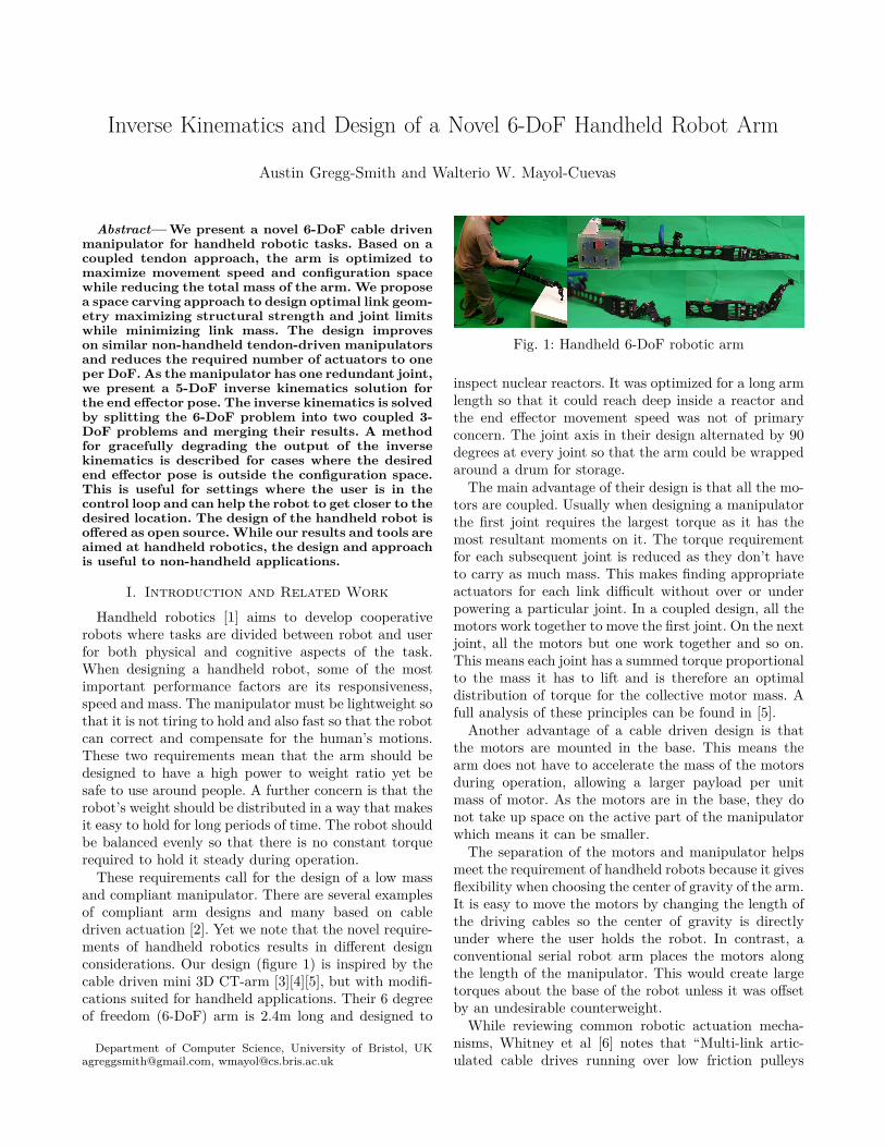
These requirements call for the design of a low massand compliant manipulator. There are several examplesof compliant arm designs and many based on cabledriven actuation [2]. Yet we note that the novel require-ments of handheld robotics results in different designconsiderations. Our design (figure 1) is inspired by thecable driven mini 3D CT-arm [3][4][5], but with modifi-cations suited for handheld applications. Their 6 degreeof freedom (6-DoF) arm is 2.4m long and designed to

Department of Computer Science, University of Bristol, UKagreggsmith@gmail.com, wmayol@cs.bris.ac.uk

Fig. 1: Handheld 6-DoF robotic arm

inspect nuclear reactors. It was optimized for a long armlength so that it could reach deep inside a reactor andthe end effector movement speed was not of primaryconcern. The joint axis in their design alternated by 90degrees at every joint so that the arm could be wrappedaround a drum for storage.

The main advantage of their design is that all the mo-tors are coupled. Usually when designing a manipulatorthe first joint requires the largest torque as it has themost resultant moments on it. The torque requirementfor each subsequent joint is reduced as they don’t haveto carry as much mass. This makes finding appropriateactuators for each link difficult without over or underpowering a particular joint. In a coupled design, all themotors work together to move the first joint. On the nextjoint, all the motors but one work together and so on.This means each joint has a summed torque proportionalto the mass it has to lift and is therefore an optimaldistribution of torque for the collective motor mass. Afull analysis of these principles can be found in [5].

Another advantage of a cable driven design is thatthe motors are mounted in the base. This means thearm does not have to accelerate the mass of the motorsduring operation, allowing a larger payload per unitmass of motor. As the motors are in the base, they donot take up space on the active part of the manipulatorwhich means it can be smaller.

The separation of the motors and manipulator helpsmeet the requirement of handheld robots because it givesflexibility when choosing the center of gravity of the arm.It is easy to move the motors by changing the length ofthe driving cables so the center of gravity is directlyunder where the user holds the robot. In contrast, aconventional serial robot arm places the motors alongthe length of the manipulator. This would create largetorques about the base of the robot unless it was offsetby an undesirable counterweight.

While reviewing common robotic actuation mecha-nisms, Whitney et al [6] notes that “Multi-link artic-ulated cable drives running over low friction pulleys

and capstans offer perhaps the highest efficiency andsmoothest operation among existing mechanical trans-missions [7], [8]”. All these factors combine to give anarm that is dexterous, fast and powerful for its size.However, introducing a new arm design often results

in the need to develop specific solutions to its inversekinematics as generic solutions tend to be inefficientcomputationally and thus may limit the reaction andoperational conditions that are critical in the agile anddemanding handheld robot setting. This paper concen-trates on both the design and the Inverse Kinematics ofour handheld robot arm with section II describing themechanical design of the arm including design featuresand link optimization via space carving while section IIIdescribes the coupled solution to the inverse kinematics.

II. Mechanical DesignWhen designing a cable driven actuator the first ques-

tion is how to configure the joint axes to maximize theconfiguration space. The biggest constraint is that thewires from the joint closest to the end effector must passthrough the rest of the arm with minimal friction whilsteliminating wire collisions. This constraint dominatesthe design process when attempting to maximize theindividual joint limits.

While it is possible to have axial motion transmittedvia a cable differential as in the WAM arm [8], the designis mechanically complex and does not fit well with acoupled design. For this reason we restricted the joint’saxes to two directions. We iterated through possibleconfigurations with these joint axis limits using physicalprototypes before deciding on the configuration shownin figure 2. One advantage of this design is that the axesof adjacent joints are always parallel except betweenthe third and fourth joint. This minimizes cable wearand friction as the driving tendons don’t have to changedirection more than strictly necessary. The configurationof two serially connected three link segments also allowsfor a inverse kinematics solution that takes advantage ofthe repeated structure as discussed in section III.

Fig. 2: Joint configurationA. Design Features

1) Minimizing Actuator Requirements: The 2.4m longMini 3D CT-Arm [5], uses 12 motors to control 6 degreesof freedom. They use pairs of motors to apply tensionto each side of the wire for each of the 6 pulleys.Our design uses half the number of motors, so thatone motor is directly linked to a corresponding pulley.The CT-arm uses potentiometers to measure the jointangles of each link but because the new arm has themotors directly coupled to each pulley, there is no longera need for potentiometers as the relationship between

motor angles and joint angles is fixed. This is in partpossible because the arm is much smaller (30cm vs240cm) so the elasticity of the tendons is less critical.These two improvements reduce weight and complexitysignificantly. Figure 3 shows the wiring configurationfor all the joints and a model of the assembled arm.The green cylinders indicate motor driven pulleys, whilethe turquoise and blue cylinders show the link drivingpulleys. The wires are shown wrapped around invisibleidler pulleys to make the wiring clearer. The spacingbetween the wires has been expanded for clarity sothe large angles the wires take between pulleys in thediagram are not representative of the built arm.

Fig. 3: Arm model and wiring diagram. The green cylin-ders indicate motor driven pulleys, while the turquoiseand blue cylinders represent the link driving pulley. Thebase link is labeled l0 and subsequent links incrementby one to give l1, l2 etc. θ1 is the angle between l1 andl0 and follows the same incrementing naming scheme asthe links.

2) Link Design Via Space Carving: The arm jointconfiguration is comprised of a first section with threeparallel joint axes, followed by a second section withthree more joint axes rotated by 90 degrees relative tothe first section. Figure 4 shows the configuration spaceof one of these three-link sections. The gray area is thespace reachable by the beginning of link 3 (θ3). Theouter surface of the annular area is reached when θ2 = 0and the inner edge when θ2 is at the maximum allowedangle limit (θ2max). The minimum possible distancefrom link 1 to link 3 is sin

(π−θ2

2)

2L. This distance isminimized when θ2 is maximized so in order to have alarge configuration space, it is important to maximizethe joint limits of θ2. In figure 4 right where θ2 = θ2max, in order to keep link 3 in the same axis as the base link,θ1 = θ3 = − θ2max

2 , so maximizing these joint limits has asmaller effect on the size of the configuration space . It isstill advantageous to maximize the other joint limits asmuch as possible, as they will increase the configuration

space, but they are of secondary priority.

Fig. 4: Analysis of the workspace of a 3R arm used tooptimize the joint limitsThe same calculations apply to the second three link

section for joint angles θ4, θ5, θ6. With this in mind,the links were designed to maximize the joint limitsfor θ2 and θ5 as a first priority and then to maximizethe remaining limits where possible. The other criteria— minimizing size and mass while maximizing strengthand rigidity — are at odds with maximizing joint limitsbecause of the constraints large joint limits have onwhere material structure for the link can be placed.

To maximize both criteria, a form of space carving wasused. When designing a link, the two connecting linksare moved through their joint range to cut out the sweptvolume. The remaining material makes up the centralcore of the link as shown in blue in figure 5a. Figure5b and 5c shows two CAD models of links producedusing this technique. The middle shows link 3 which usesthe same carving principle but has more complicatedgeometry due to the change of joint axis. An advantageof this technique is that adjacent links fit each otherperfectly when they are at their maximum joint limitsso the arm can be folded up into a compact and safeconfiguration during transportation.

Using this method the joint limits are as follows:θ1max = ±135◦ , θ2max = ±150◦, θ3max = ±135◦,θ4max = ±125◦, θ5max = ±150◦, θ6max = ±150◦.

max angle

min angle

max angle

min angle

(a) (b) (c)

Fig. 5: Space carving method for minimizing link ma-terial. a): Material that is not carved away by rotatingadjacent links is left in blue. b) and c): CAD modelsof link 1 and link 3 designed by using a space carvingtechnique.

B. HardwareThe prototype arm links were 3D printed in ABS and

the idler pulleys machined out of aluminum. The CADfiles for all the components are open source and madeavailable at [9]. The robot is powered by six Dynamixel

MX-64T servos mounted on cable tensioning mecha-nisms. After the links and pulleys have been assembled,the driving cables are attached directly to each motor.The motors are mounted on a 3D printed saddle that fitsinto a corresponding bed shown disassembled in figure6a. The motor is moved forward and backward in the bedby a bolt that acts as a lead screw. Figure 6b illustrateshow the motors are arranged in a sideways “V” forma-tion so that the motors can be individually tensionedwithout the cables crossing. When the arm is first turnedon, it is calibrated by controller firmware recording theoffset between the known zero angle of the arm, andthe current angle recorded by the motor encoders. Thiscalibration must be repeated every time the cables arede-tensioned or re-tensioned during maintenance.

The arm is used in an assisted inspection task wherea user holds the robot and the actuated end effectorautonomously seeks unexplored inspection zones [10].The end effector can reach around obstacles with itstentacle-like design. The manipulator is also suitable forassisted pick and place, and/or painting tasks.

(a) CAD model of dis-assembled tensioner

(b) CAD model of the sideways“V” shaped servo layout with ca-bles shown in red

Fig. 6: Cable tensioning mechanism and layout

III. 6-DoF Inverse Kinematics using coupled3-DoF solutions

Although general purpose computational inverse kine-matic (IK) solutions exist [11], [12] there are severaladvantages to an analytical solution. Although therehave been performance improvements for computationalmethods, they are still generally based on algorithmsthat iteratively converge on a solution given some start-ing conditions and so are more computationally intensivethan an analytical approach. Inverse kinematics prob-lems often have multiple solutions but a computationalalgorithm will generally only return the solution that isnearest to the input starting solution. This is an undesir-able characteristic when using the IK results as the inputto a path planner because the solution that convergesfrom the IK might not be the configuration that givesthe best results from the path planner. An analyticalsolution will provide all the valid configurations thatreach a pose which gives the path planner more optionsto find short paths to that pose.

Figure 7 shows the nomenclature used when solvingthe inverse kinematics problem. L is defined as the line

Fig. 7: Planes for solving each 3-DoF problem. Thebase plane is in red and the tip plane is in green. Theinverse kinematics is solved in 2D on each plane for thecorresponding section of 3 parallel joints. Their resultsare merged along the common line between the twoplanes where they intersect.

common to both the plane defined by the base of therobot (red) , and the plane defined by the desired endeffector pose (green). The kinematics of the arm has oneredundant joint so in most cases there are an infinitenumber of positions where l3 can lie along L while l0and l6 stay fixed. Practically, this means you can slidel3 forward and backwards along L until l3 collides withanother link or reaches one of the joint limits. The mainproblem when solving the inverse kinematics is choosingthe optimum position for l3.The arm is made up of two sets of joints that have two

common axes of rotation. The first set is defined as allthe joints and links that lie on the base plane pb whichare B = {θ1, θ2, θ3}, {l0, l1, l2, l3} while the second setE = {θ4, θ5, θ6}, {l3, l4, l5, l6} all lie on the end effectorplane pe shown in green. Note that l3 is contained byboth sets and lies on line L which is defined by where pband pe intersect. The 6-DoF problem can be split intotwo 3-DoF problems defined by B and E that each lieon their own plane.Problem B : Given the pose of l0 and L, where can l3

lie on L without any collisions between l0, l1, l2, l3 andkeeping θ1, θ2, θ3 within their joint limits?

Problem E : Given the pose of l6 and L, where can l3lie on L without any collisions between l3, l4, l5, l6 andkeeping θ4, θ5, θ6 within their joint limits?

The solution to each problem is a list of possiblelocations that l3 can occupy. When both B and E havebeen solved, the position of l3 is chosen as all locationswhere the valid locations overlap. This ensures thatall collision constraints and joint angle limits are met.Once the position of l3 is known the problem is fullyconstrained and it is straightforward to solve for thejoint angles θ1, θ2, θ3, θ4, θ5, θ6 using geometry.B and E are essentially the same problem but with

the direction and associated links reversed. We define afunction:

l3 = ik3D(lfixed, la, lb, lonLine, L, θaMax, θbMax, θcMax)

Problem B is expressed as:

l3 = ik3D(l0, l1, l2, l3, L, θ1Max, θ2Max, θ3Max)

and problem E as:

l3 = ik3D(l6, l5, l4, l3, L, θ6Max, θ5Max, θ4Max)

Section III-A explains how to calculate the joint andlink collision constraints. Section III-B shows how toenumerate possible locations for l3 given the collisionconstraints and section III-C merges the results of Band E into a 6-DoF solution.

A. Calculating Valid 3-DoF Solution BoundariesThe black line with the arrow in figures (8-14) is

the a “line query” which is 2D projection of L andindicates the direction and range of positions l3 mustlie on. Figure 8 illustrates the links and their associatedjoint limits which are color coded the same way acrossall the diagrams mentioned above. In this section, thegeometry will be discussed in terms of problem B withθ1, θ2, θ3, l0, l1, l2,l3, but the same logic applies to prob-lem E where l0 is replaced by l6, l1by l5, etc and θ1 byθ6, θ2 by θ5, etc.

Fig. 8: Both link’s are collinear boundary

If joint limits and link-to-link collisions are ignored,the inverse kinematics solution for the 3 joint sectionis trivial and well known [13]. In figure 8, l3 would beable to reach any location inside the gray circle andtherefore any point where L is inside the circle. If theangle and collision constraints are added this is no longerguaranteed to be true and more analysis must be done.

Figure 8 shows the simplest example of a boundarycondition. The two boundaries of where l3 can lie are atthe intersection points of the gray circle and L. Figure 8right shows all the places that l3 can lie on L in magenta.The link configurations to reach the magenta points aredrawn in a lighter color for clarity.

In the following section we describe how to calculatethe boundary solutions for seven different joint andcollision constraints. Once all the boundary conditionshave been described, we will explain how to combinetheir results.

The seven boundary constraints are:1) l1 and l2 are collinear: 2 solutions (figure 8)

2) θ1 = θ1max : 4 solutions (figure 9)3) θ2 = θ2max : 4 solutions (figure 10)4) θ3 = θ3max : 4 solutions (figure 11)5) l2 collides with l0: 2 solutions (figure 12)6) l3 collides with l0: 2 solutions (figure 13)7) l3 collides with l1: 1 solution (figure 14)1) Links 1 and 2 are Collinear: The first and simplest

case is where the l1 and l2 lines are collinear as shownby figure 8. The two possible solutions are found at theintersection between L and a circle with radius = 2llen. The third link is shown in orange and is collinear withL and points in the same direction. In the subsequentexamples l3 is not always shown because it often makesthe diagram harder to understand, but it should beassumed to be there.

2) Joint 1 Constraints: Figure 9 right shows fourpossible solutions where θ1 is at its maximum range oftravel. l1 can have two possible locations when θ1 =±θ1Max. For each of these two locations, the validlocations for l3 are the intersection point of the L and thecircle defined by the radius = llen as shown by figure 9left. In this example, two of the four solutions have beenrejected because they are past the joint limits of θ3 andare draw in gray.

θ3

θ3

θ1

l3

l3

l3

l3

Fig. 9: Joint 1 at maximum limit boundary

3) Joint 2 Constraints: Figure 10 left shows the con-struction method for calculating the solutions where θ2is at it’s maximum range. A triangle ABC is constructedwith two sides of length = llen and angle ABC setso that θ2 is at its maximum angle. The length of thethird side defines the radius R of the circle (black) thatall the valid solutions must lie on. The positions of l3are the points where the circle intersects L. Figure 10right shows the same configuration, but shows all fourcandidates including the two invalid solutions (gray)that are rejected because they exceed the joint limitsof θ1 or θ3. Note that the reachable areas are theregions of L that are outside the black circle shownin magenta because inside the circle is the region thatbreaks the constraints of θ2. The same is true for theother boundary conditions but it is difficult to showgraphically so they are omitted from the diagrams.

AR

C

θ1θ3

B

l3

l3 θ2

Fig. 10: Joint 2 at maximum limit boundary

4) Joint 3 Constraints: Figure 11 right shows fourpossible solutions where θ3 is at its maximum anglerelative to L. In figure 11 left the angle LDE is setfrom the maximum θ3 angle and is used to calculatelength N. Lines La, Lb are offset from L by length N.The intersection points between La and Lb and circle Care the candidate positions for θ2. Figure 11 right showsthe two solutions shown in gray that were rejected forexceeding the maximum angle of θ2.

La LbL

D

E N

C

θ2

θ2θ3

θ3

θ3

θ3

Fig. 11: Solutions where joint 3 is at its maximum limitboundary

5) Link 2 Collides with Link 0: Figure 12 left showsthe case where l2 collides with l0. l3 must lie on theintersection point of L and l0. The possible positions forθ2 are the intersections between the blue circle and thegreen circle. Figure 12 right shows all possible solutionsincluding the grayed out one rejected for exceeding θ3angle limits.

θ2

θ2

θ3

Fig. 12: Link 2 collides with link 0

6) Link 3 Collides with Link 0: Figure 13 shows thecase where l3 collides with l0. The intersection of L andl0 is found. l3 must then be 1 link length backwardalong L from the intersection point. A blue circle is

constructed around this point and intersected with thegreen circle around l0 to find the two candidates for θ2.Figure 13 right shows a valid solution and an invalidsolution that exceeds θ1 angle limits.

θ2

θ2

θ1

Fig. 13: Link 3 collides with link 0

7) Link 3 Collides with Link 1: The last case cannotbe solved using geometric constraints alone. Given theconstraints that the end of l3 must touch l1 and alsolie on L, there is no closed form solution for the jointangles that meets these constraints, as shown in figure14 right. In order to calculate the position of any link,the position of one of the other links must be knownalready. For example, the angle of θ1 cannot be knownwithout knowing how far along L l3 lies, but the positionof l3 is dependent on the angle of θ1.

QPR

D

G

H

C

L

F θ1

θ2

Fig. 14: Link 3 collides with link 1

Instead an interpolation method was used to calculatethe link configuration that meets all these constraints asshown in figure 14. A list of valid solutions are generatedby calculating the forward kinematics of a series of jointangles that match the constraints. When looking at thisproblem from a forward kinematics perspective, the aimis to produce an isosceles triangle PQR, where angleRPQ and angle QRP have the same magnitude. Togenerate this set of valid isosceles triangles the followingjoint angles are chosen:

θ1 = 0, θ2 ∈ [j3Max/2,23π], θ3 = 2(π − θ2) (1)

Once all the link positions have been calculated aline L is constructed to lie on l3. Iterating through theforward kinematics gives us a mapping of joint anglesto the line L. To solve the inverse problem, we wantto know the joint angles given an arbitrary line L. Theproblem is constrained enough that if we can calculatethe mapping from L to the angle of θ1, θ2 or θ3, wecan work out the rest of the geometry through normalgeometric constraints.

In this example, we chose to solve for θ1 as a functionof L, where L is parametrized as a 2D position anddirection:

θ1 = f(L) = f(px, py, dx, dy) (2)

At first glance it appears that the interpolation functionwill require four inputs to describe the directed line,however the problem can be constrained to 2-DoF. Theline L is constrained so that it must touch the circle Cat two points (G,H) so the line can be parametrized bythe angle GDH and FDH.

θ1 = f(GDH,FDH) (3)

This is still 2-DoF and for simplicity it would be betterto only interpolate over a 1D function instead of 2D. Ifthe angle GDH stays constant and angle FDH changes:

θ1 = PDH − FDH (4)

To solve for the angle of θ1 using PDH, we create aninterpolation function from equations (2), (3), and (4)that accepts angle GDH and returns PDH.

PDH = f1(GDH) (5)

Combining equations (3), (4), and (5) gives:

θ1 = f(GDH,FDH) = f1(GDH)− FDH (6)

Once θ1 angle is known, the position θ2 can be calculatedusing trigonometry. The position of l3 is the intersectionof a circle around θ2 and the line L. The problem is thenfully solved.

B. Calculating Valid 3-DoF Solution Ranges

The previous section covered the seven behaviors thatmark the boundaries of sets of solutions given differentconstraints. In some cases, all the solutions on one sideof the boundary solution will be valid and on the otherside will be invalid. The other case is where the solutionswill be valid on both sides of a boundary. Regardless,the regions of valid solutions are always enclosed by apair of solutions calculated above. In order to calculatethe range of valid solutions, the spaces between thecalculated boundaries are tested and classified as validor invalid.

(a) (b) (c) (d)

Fig. 15: A list of L queries and the corresponding validsolution rangesFigure 15 shows valid ranges of solutions for a number

of desired line queries. Part (a) shows the simplest case;where the boundary solutions are both straight lines.The valid solutions between the boundary cases areshown in a lighter color and the point where they meetthe desired line is highlighted in magenta. As the desiredline moves to the left, part (b) shows that the topboundary condition remains “collinear” but the bottom“collinear” has been replaced by “joint2” because giventhe current L, the collinear solution is no longer validand has been replaced by a “joint2” solution. An extra“joint2” solution is also now valid in the middle of theline but since there are valid solutions to either side ofthe “joint2” it does not mark a reachability boundary.Part (c) shows that as L moves further to the left,the once continuous magenta region is now split intotwo separate segments. Starting from the bottom of(c), the first segment is surround by the “joint2” and“joint1” boundary conditions while the second segmentis contained by “joint1” and “collinear” boundaries. Theregion of L between these two segments is not reachableas at least one of the seven constraints are not met. Sec-tion (d) shows the first valid region between “joint2” and“joint1” get split by a pair of “joint0” boundaries, whilethe second valid region from (c) remains unchanged. Theprocess of calculating the valid regions is the same forany desired line query.

C. Merging Valid 3-DoF Solution RangesUp until this point, we have only been considering the

solution of a 3-DoF problem. As described in section III-A the 6-DoF problem can be considered as consistingof two 3-DoF problems taking place in two differentorthogonal planes.

Figure 16 shows the output of two sets of two 3-DoFproblems and their overlapping sections. The 3-DoFproblem has to be solved four times because directionof l3 is important for the constraints. First l3 is chosento face to the right while lying on L and the 3-DoFproblem is solved once for the base plane.Next we draw the magenta region described in the

previous section as red rectangles with arrows facing tothe right on the far side of L. The same is done forthe end effector plane, whose valid regions are drawn as

Fig. 16: Base (red) and tip (green) valid solution rangesare shown as boxes with arrows indicate the direction ofthe common link. Blue boxes show the overlap betweenthe base and tip ranges. Right: One valid solution. Left:All valid solutions

green rectangles with arrows facing to the right. Then wereverse the direction of l3 and solve the problem again forthe base and end effector planes. The results are shownas green and red rectangles on the near side of L witharrows facing to the left.

At this point, all of the constraints for both the baseand end effector sections are described in a commonreference frame and they can now be merged to finda global solution. The blue rectangles are regions ofoverlap between the valid base ranges (red) and validend effector ranges (green). l3 must lie somewhere insidethe blue range to meet the combined constraints of boththe base and tip sections.

In figure 16 left the solution shown in gray is onlyone of many possible solutions. Each of the calculatedblue ranges has an infinite number of solutions so onlythe midpoint of the range is chosen as the output ofthe function. The midpoint is chosen rather than eitherend of the range because it distributes the magnitudeof the joint angles more evenly across all the joints.Figure 16 right shows the same configuration as figure16 left but with all valid midpoints of the blue solutionsplotted. In this case there exist six solutions, but it ispossible to have up to the (number of ranges) ×(numberof directions) ×(number of base solutions) ×(number ofend effector solutions) = 3× 2× 2× 2 = 24 solutions.

When operating in an unconstrained environment, itis often sufficient to choose the solution that is closestto the current configuration of the arm. However, ifthere are obstacles that the robot must avoid, someof the calculated solutions will be invalid due to thelinks colliding with the environment. In this case a pathplanning algorithm can use all the possible solutions andchoose the one that minimizes collision.

D. Solution’s Graceful DegradationThe above sections describe the solution to the 5-DoF

inverse kinematics problem. However there are caseswhere the arm does not have a 5-DoF solution to adesired pose. In these cases it is desirable that the outputof the inverse kinematics function should return the

(a) 5-DoF (b) 5-DoF boundary (c) 4-DoF (d) 3-DoF (e) 2-DoF

Fig. 17: Graceful degradation offers as IK output the closest pose to guide the user and implicitly prompts for helpin reaching the goal

closest possible pose. We call this graceful degradationand it is achieved by reducing the number of DoF thatthe end effector attempts to reach as illustrated in figure17. From the user’s perspective of holding the robot asa handheld tool, this is intuitive as the reduced solutioncan be interpreted as a pointing gesture by the robot, toindicate where the user should move the robot towards.The desired end effector pose is a position ep and

direction ed and drawn as a black arrow in figure 17.Figure 17a shows the arm reaching the desired posesuccessfully. Note that θ3 is inside the red base circle cbdefined about the center of θ1 with radius = 2llen andθ4 is inside the end effector circle ce centered about θ6shown in green. In this case, there are two ways for thebase links to reach l3 (shown in cyan and orange), andtwo ways for the end effector links to reach to l3 (shownin cyan and purple). In (b) the desired pose has movedup on the gray cuboid and θ4 is now touching the edgeof ce. This causes the two end effector solutions shownin (a) as cyan and purple to collapse to the one shown incyan in (b). This is the boundary between 5-DoF and 4-DoF solutions, because if the desired pose moves fartherup the cube there are no more valid 5-DoF solutions andonly 4-DoF can be reached, as illustrated in (c).The desired end effector direction ed can be

parametrized by pitch and yaw angles defined relativeto the base. Once the end effector pose is too far awayto reach with 5-DoF it is still possible to reach ep if thedesired pitch or yaw constraints of ed are relaxed. Infigure 17c, l6 is not longer collinear with ed because thepitch constraint is not met but the yaw constraint is stillmet because l3 still lies on L.In figure 17d l3 does not lie on L any more so both

the pitch and yaw constrains are not met and only the 3-DoF ep has been reached. Note that in (c) there are twobase plane solutions (shown in orange and cyan) thatcollapse down to one solution in (d) where θ3 cannot lieon the intersection of cb and L, so it now lies on the edgecb that is closest to ep.If ep moves further up the gray box it moves entirely

out of range of the arm so that only θ1 and θ4 arerequired to move the end effector as close as possible toep resulting in a 2-DoF solution. In figure 17, the pitchconstraint is relaxed before the yaw constraint becauseep moves such that θ4 hits the edge of ce before θ3 hitsthe edge of cb. However if ep is moved towards us, theyaw constraint will need to be relaxed before the pitch

using the same principles outlined above.

IV. ConclusionsWe present a novel design optimized for the nascent

area of handheld robotic applications through the useof link to link space carving. The inverse kinematics aresolved analytically by splitting the 6-DoF problem intotwo coupled 3-DoF problems and merging the results.A method for gracefully degrading the number of DoFthat the arm reaches when the desired end effector poseis outside the arm’s configuration space is also proposed.The arm design and CAD files are released as opensource hardware at [9].

References[1] A. Gregg-Smith and W. W. Mayol-Cuevas, “The Design and

Evaluation of a Cooperative Handheld Robot,” in ICRA,2015.

[2] R. J. Webster and B. A. Jones, “Design and KinematicModeling of Constant Curvature Continuum Robots: AReview,” The International Journal of Robotics Research,vol. 29, no. 13, 2010.

[3] S. Ma, S. Hirose, and H. Yoshinada, “Design and experimentsfor a coupled tendon-driven manipulator,” IEEE ControlSystems, vol. 13, no. 1, feb 1993.

[4] S. Hirose and S. Ma, “Coupled tendon-driven multijointmanipulator,” in ICRA 1991, 1991.

[5] A. Horigome, H. Yamada, G. Endo, S. Shin, S. Hirose, andE. F. Fukushima, “Development of a Coupled Tendon-Driven3D Multi-Joint Manipulator,” in ICRA, 2014.

[6] J. Whitney, M. Glisson, E. Brockmeyer, and J. Hodgins, “ALow-Friction Passive Fluid Transmission and Fluid-TendonSoft Actuator,” in IROS, 2014.

[7] S. Charles, H. Das, T. Ohm, C. Boswell, G. Rodriguez,R. Steele, and D. Istrate, “Dexterity-enhanced teleroboticmicrosurgery,” in ICAR, 1997.

[8] Townsend W and Salisbury J, “Mechanical design for whole-arm manipulation,” in Robots and Biological Systems: To-wards a New Bionics? Springer, 1993, pp. 153–164.

[9] “http://www.handheldrobotics.org.”[10] A. Gregg-Smith and W. W. Mayol-Cuevas, “Investigating

Spatial Guidance For a Cooperative Handheld Robot,” inICRA, 2016.

[11] A. Aristidou and J. Lasenby, “FABRIK: A fast, iterativesolver for the Inverse Kinematics problem,” GraphicalModels, vol. 73, no. 5, sep 2011.

[12] R. Mukundan, “A Fast Inverse Kinematics Solution for ann-link Joint Chain,” ICITA, 2008.

[13] J. J. Craig, Introduction to Robotics Mechanics and Control.Prentice Hall, 1985.