green box subsidies: a theoretical and empirical...

1

CONFÉRENCE DES NATIONS UNIES SUR LE COMMERCE ET LE DÉVELOPPEMENT

UNITED NATIONS CONFERENCE ON TRADE AND DEVELOPMENT

Green Box Subsidies: A Theoretical and Empirical Assessment

By UNCTAD India Team

May 2007

Critical Appraisal by* Joseph Stiglitz (Colombia University), Andrew Charlton(Centre for Economic Performance, LSE), David Abler (Pennsylvania State University) Comments on an Earlier Draft* Tim Josling (Stanford University)

Prepared under UNCTAD- Govt. of India- DFID Project ‘Strategies and Preparedness for Trade and Globalization in India’.

The views expressed in this paper do not reflect the views of UNCTAD or it’s member states. This is an unedited version of the paper.

Please send your comments to [email protected]

* All the comments by the reviewers have been taken into consideration and incorporated in the paper.

2

This paper has been brought out under the aegis of the Project Strategies and

Preparedness for Trade and Globalization in India which UNCTAD has been

implementing since March, 2003. The Ministry Of Commerce, Government of India

is a co-partner of the project which is being supported by the Department for

International Development (DFID), Government of UK. The project has two main

inter-related components. The first component seeks to assist Indian trade

negotiators, policy makers and other stakeholders in enhancing understanding of the

development dimension of key trade issues. The second component seeks to

strengthen human and institutional capacities, as well as a policy environment that

will support and sustain a more equitable process of globalization. The project seeks

to build institutional and human resource capacities so as to gain from globalization;

to mitigate its negative effects as well as influence the planning and policy making

processes.

3

Table of Contents INTRODUCTION 9 I. THEORETICAL DEBATES AROUND GB MEASURES 12

Criteria for GB Subsidies....................................................................................................... 12 Government service programmes .......................................................................................... 12 Direct payments to producers ................................................................................................ 13 Theoretical debates on GB Measures .................................................................................... 13 Wealth and risk effects........................................................................................................... 13 Insurance effects .................................................................................................................... 16 Cost, price and expectation effects ........................................................................................ 17 Productivity Effects ............................................................................................................... 19 Conclusion ............................................................................................................................. 20

II. ANALYSIS OF GB MEASURES OF THE UNITED STATES, EUROPEAN UNION AND JAPAN 21

Overall Structure of Domestic Support for the US, EU and Japan........................................ 21 Category wise Expenditure on GB by the US, EU and Japan ............................................... 24 General Services .................................................................................................................... 24 Public Stockholding for Food Security Purposes .................................................................. 25 Domestic Food Aid ................................................................................................................ 26 Decoupled Income Support.................................................................................................... 26 Income Insurance and Income Safety Net Programmes ........................................................ 28 Payments for Relief from Natural Disaster............................................................................ 29 Structural Adjustment through Producer/Resource Retirement Aids.................................... 29 Structural Adjustment through Investment Aids ................................................................... 30 Environmental Programme Payments.................................................................................... 30 Regional Assistance Programmes.......................................................................................... 31 Conclusion ............................................................................................................................. 32

III. DEA ANALYSIS AND CGE MODELLING 33 Data Envelopment Analysis (DEA) Estimation .................................................................... 33 Malmquist TFP Indices.......................................................................................................... 35 Estimation of TFP Changes ................................................................................................... 36 Estimation of Cost Efficiencies ............................................................................................. 38 Stochastic Frontiers................................................................................................................ 42 CGE Modelling...................................................................................................................... 45 Conclusion ............................................................................................................................. 53

IV. TRANSLOG AND COBB DOUGLAS COST ESTIMATES 54 Translog Cost Function.......................................................................................................... 54 Variables and Data Sources ................................................................................................... 55 Translog Cost Specification with regard to Total GB Subsidies ........................................... 56 Translog Cost Specification with regard to General Services ............................................... 58 Translog Cost Specification with regard to Environmental Services .................................... 59 Translog Cost Specification with regard to Decoupled Payments......................................... 61 Crop-Wise Results ................................................................................................................. 62 Variables and Data Sources ................................................................................................... 63 Empirical Results ................................................................................................................... 63 Wheat ..................................................................................................................................... 65 Corn........................................................................................................................................ 66

4

Rice ........................................................................................................................................ 66 Soybean.................................................................................................................................. 67 Cotton..................................................................................................................................... 67 Conclusion: Summarizing the results of the Empirical Analysis .......................................... 68

V. REVIEW AND CLARIFICATION OF GB CRITERIA: PROGRESS IN NEGOTIATIONS 70

Mandate for review and clarification of GB criteria: The July Framework and the Hong Kong Declaration .............................................................................................................. 70

Assessment of GB proposals ................................................................................................. 72 Suggestions for further proposals .......................................................................................... 74 Conclusion ............................................................................................................................. 75

VI. CONCLUSIONS 77 APPENDIX-181

Data Envelopment Analysis (DEA)....................................................................................... 81 1. Output Oriented DEA ........................................................................................................ 82 2. Malmquist DEA analysis ................................................................................................... 83 3. Cost Efficiency Analysis Using Input Oriented Method ................................................... 83

APPENDIX-286 CGE-GTAP Methodology and Aggregations 86

Computable general equilibrium analysis.............................................................................. 86 Salient features of the CGE model......................................................................................... 86 Database................................................................................................................................. 87

APPENDIX-392 State of Play of WTO Negotiations on GB............................................................................ 92 (i) General Services................................................................................................................ 92 (ii) Public stockholding for food security purposes............................................................... 92 (iii) Domestic food aid ........................................................................................................... 92 (iv) Direct payments to producers.......................................................................................... 93 (v) Decoupled income support............................................................................................... 93 (vi) Income insurance and income safety- net programmes .................................................. 94 (vii) Payments for relief from natural disaster ....................................................................... 95 (viii) Structural adjustment assistance through producer/ resource retirement programmes 95 (ix) Structural adjustment assistance through investment aids .............................................. 95 (x) Payments under regional assistance programmes ........................................................... 96

REFERENCES 98

List of Tables Table 1 Structure of Domestic Support for the US, EU and Japan (in Domestic Currencies).22 Table 2 Expenditure on General Services in the US, EU and Japan (in US $ billion). ........... 24 Table 3 Expenditure on Public Stockholding for Food Security Purposes in the US, EU and

Japan (in US $ million) ...................................................................................................... 25 Table 4 Expenditure on Domestic Food Aid in the US, EU and Japan (in US $ million)....... 26 Table 5 Expenditure on Decoupled Income Support in US, EU and Japan (in US$ million). 27 Table 6 Expenditure on Income Insurance and Income Safety Net Programmes in the US, EU

and Japan (In US million Dollars) ..................................................................................... 28 Table 7 Expenditure on Payments for Relief from Natural Disaster in US, EU and Japan (in

US$ million)....................................................................................................................... 29 Table 8 Expenditure on Structural Adjustment through Producer/Resource Retirement Aids in

US, EU and Japan (in US$ million)................................................................................... 30

5

Table 9 Expenditure on Structural Adjustment through Investment Aids in US, EU and Japan (in US$ million) ................................................................................................................. 30

Table 10 Expenditure on Environmental Programme Payments in US, EU and Japan (in US$ million)............................................................................................................................... 31

Table 11 Expenditure on Regional Assistance Programmes in US, EU and Japan (in US$ million)............................................................................................................................... 31

Table 12 Average GB Expenditure (US$ million) 1995–2000. .............................................. 35 Table 13 Mean of Total Factor productivity, Technical Efficiency and Technical Change with

GB Expenditures (Malmquist Indices). ............................................................................. 36 Table 14 Change in TFP, Technical Change and Change in TE due to GB Expenditures (per

cent): 1995 to 2000. ........................................................................................................... 37 Table 15 Decomposition of GB Expenditures. ........................................................................ 39 Table 16 Cost efficiency and Change in Cost Efficiency with GB Expenditure (Deterministic

DEA). ................................................................................................................................. 41 Table 17 Cost efficiency and Change in Cost Efficiency with GB Expenditure..................... 44 Table 18 Effect of GB subsidies on Production and Trade (percentage change) .................... 46 Table 19 Global Agricultural Output. (US$ Million) .............................................................. 47 Table 20 Employment Effect in Agricultural Sector (Percentage Change)............................. 48 Table 21 Impact on Agricultural Wages. (Percentage Change). ............................................. 49 Table 22 Sum of the Value(EVFA) Change in All Three Sectors........................................... 50 Table 23 Removal of GB Effect on Net Food Importing Countries (in percentage terms).... 51 Table 24 Production Effects for NFICs .................................................................................. 52 Table 25 Import Effects for NFICs......................................................................................... 52 Table 26 Translog Cost Function With GB Subsidies............................................................. 57 Table 27 Translog Cost Function With Subsidies On General Services. ................................ 58 Table 28 Translog Cost Function With Environmental Subsidies........................................... 60 Table 29 Translog Cost Function With Decoupled Payments................................................. 61 Table 30 Wheat. ....................................................................................................................... 65 Table 31 Corn. ......................................................................................................................... 66 Table 32 Rice ........................................................................................................................... 66 Table 33 Soybean..................................................................................................................... 67 Table 34 Cotton........................................................................................................................ 67

List of Figures

Figure 1 The Insurance Effects of Safety Nets ........................................................................ 16 Figure 2 Shift in Producer’s Equilibrium................................................................................. 17 Figure 3 Productivity Improvement & Shift in Supply Curve................................................. 20 Figure 4 Interest on Operating Capital .................................................................................... 64 Figure 5 Land Prices (US$ per ha). ......................................................................................... 64 Figure 6 Output-Orientated DEA............................................................................................. 83

List of Boxes

Box 1 Box Shifting. ................................................................................................................. 23 Box 2 Farm Reforms in the United States. .............................................................................. 23 Box 3 Farm Reforms in the European Union. ......................................................................... 27 Box 4 Various Negotiating Proposals on GB Subsidies.......................................................... 72

6

Executive Summary The Uruguay Round Agreement on Agriculture (URAA) aimed at globally reducing trade

distorting subsidies. However measures which were identified as having no or minimal trade

distorting effects were to be categorized as Green Box (GB) measures. These measures were

exempt from reduction commitments and subsidies under the GB could even be increased

without any financial limitations under the WTO.

Recent research shows that current green box subsidies do not meet the criterion of ‘no or at

most minimal’ trade distorting effects and that the so-called ‘decoupled’ programmes under

Green Box do infact distort trade. The July 2004 framework provided a mandate for review

and clarification of the Green Box criteria. At a broad level the negotiating proposals sought to

(i) make the eligibility criteria for developed countries more restrictive and. (ii) clarify/ add

additional criteria for covering programmes of developing countries that cause no or minimal

trade-distortions. The justification for making the conditions more restrictive arises if Green

Box subsidies do indeed distort production and trade.

While there is some theoretical justification for the trade distorting effects of Green Box, little

empirical work has been undertaken to substantiate this claim. Using computable general

equilibrium modelling, such as, the Global Trade Analysis Project (GTAP), and Data

Envelopment Analysis (DEA), this paper presents empirical findings that help to shed some

light onto the debate that Green Box subsidies do have significant distortive effects on trade

and production. This study has diverted from an overall welfare approach (which is often

criticised for not taking into account the distribution effects) to estimating the distributional

effects especially on the poor. Recent studies on trade and poverty such as Cline (2004)

suggest that reduction of inequalities depend on the pattern of trade liberalisation. This paper

on GB shows that the pattern of trade liberalisation through the elimination of GB would be

inequality reducing and the effects are likely to be different from tariff liberalisation.

The estimates of Green Box subsidies used here refer to the year 2000 or the nearest available

data. Subsidies provided as food aid for food security purposes or those for government

procurement or natural disaster relief have been removed from the calculations to arrive at an

adjusted Green Box subsidy estimate. These subsidies provided largely for humanitarian

7

reasons or to address the food security of lower income groups, even if trade distorting, may

need to be retained. Hence only the adjusted GB subsidy has been used in the computations in

this paper.

DEA shows that the reduction of Green Box subsidies increases the cost of production in

relative terms in countries such as Japan, Switzerland, EU and the US by about 15–30 per cent.

Plugging these results into the GTAP model, significant trade and production effects are

observed at a global level.

The paper shows that reduction of Green Box subsidies would leave global agricultural output

virtually unchanged, registering a marginal increase of 0.13 per cent, seriously challenging the

argument that reduction of subsidies would lead to a decline in global production. The largest

decrease in output is seen in the EU, US, Canada, and Switzerland. The decline in output

would be lowest in the United States perhaps because its Green Box subsidies are mostly

directed to food aid. Conversely, most developing countries can expect to increase their

agricultural output with reductions in Green Box subsidies, with Brazil, Chile, Thailand,

Morocco, South Africa and Malaysia as frontrunners. Even the Least Developed countries

(LDCs) would find their agricultural output increase by 3 per cent. These results demonstrate

the viability of the redistribution of global output in favour of competitive agricultural

producers especially developing countries consequent to the elimination of Green Box

subsidies.

Further, the paper showcases how exports from developing countries and even the least

developed countries can register an increase while overall global trade goes down on account

of decline in exports of EU, US, Canada etc. Competitive developed countries such as

Australia also stand to gain from removal of Green Box subsidies. United States, EU, and

Canada would find their exports decline by about 40 per cent or more, whereas Switzerland

and Japan would see their exports decline by over 60 per cent. Most developing countries

would find that their exports register an increase of about 20 per cent. Even LDCs would find

their exports go up by 20 per cent. Australia would see its exports go up by over 16 per cent.

As global imports decline, most countries would also show a lower dependence on agricultural

imports. Switzerland, EU and Canada can be expected to register the highest declines of over

20 per cent. The changing pattern of international trade would also help to meet the

8

development objectives of the Doha Work Programme and in addition have positive livelihood

effects. Agricultural employment would rise in almost all developing countries, while that in

developed countries, especially those providing Green Box subsidies would fall. Wages would

also rise by about 1 per cent on an average in developing countries with LDCs registering the

highest increase. Further, the sum of the value (wage times quantity) of employment across all

three sectors is positive in all developing and least developed countries. This implies that the

poverty attenuating effects of the reduction of Green Box subsidies would be positive and

significant.

To cross check the results the cost functions for five major crops in the United States has been

estimated. A translog cost function using a panel data for the period 1975–2004 shows that if

GB subsidies were to be removed cost of production would go up by 16 per cent. As far as

specific components are concerned if general services and environment services were to be

removed the cost of production would increase by 11 and 16 per cent respectively. If

decoupled payments were to be removed the cost of production would increase by 4.6 per cent.

The paper also shows that the cost of production of different crops would rise between 1 and

7% if GB subsidies were to be removed. Crops like wheat , corn and rice which are of

maximum production and export interest to developing countries show the highest increase in

cost when GB subsidies are removed. For all crops environmental subsidies are shown to be

most sensitive to the cost of production.

To sum up, this paper provides preliminary evidence supporting the argument that Green Box

subsidies are production and trade distorting. It indicates that effects of reduction of Green

Box subsidies would be positive for developing countries including the LDCs. Further these

effects would lead to poverty alleviation as it would impact the most vulnerable sections of

society positively. It is therefore recommended that the current negotiations address the issue

of eligibility of criteria of Green Box subsidies in developed countries on an urgent basis, with

a view to restricting them.

9

INTRODUCTION An important objective of the Uruguay Round Agreement on Agriculture is to reduce domestic

measures of support that distort international trade and production in agriculture. But not all

domestic support measures were deemed to be trade distorting and some of these measures

considered to have no or minimal trade distorting effects were categorized as Green Box (GB)

measures. Such measures were and are exempted from reduction commitments and can even

be increased without any financial limitation under the WTO. Annex 2 of the Agreement on

Agriculture sets out a number of general and measure-specific domestic support criteria which,

when met, allow measures to be placed in the GB. These measures can be provided by both

developed and developing countries. They must be provided through a publicly-funded

government programme (including government revenue foregone) not involving transfers from

consumers and must not have the effect of providing price support to producers.

However, recent research shows that in some instances current GB subsidies do not meet the

criteria of ‘no or minimal trade distortion’1. Studies have shown that the so-called ‘decoupled’

programmes under GB could distort trade. A large amount of money paid to farmers,

decoupled with current production, nevertheless is likely to distort trade and production

because of the wealth and risk effects associated with it. This problem is further compounded

as these payments are not transitory measures, and are therefore permanently incorporated into

the cash flows of farmers, thereby increasing their creditworthiness and serving as an

instrument for hedging against risk. In addition, the practice of updating base acres, number of

heads and payment yields, as well as changing eligible crops under Farm Assistance

Programmes, tend to raise expectations of future assistance thereby influencing their future

production decisions. Other important channels through which direct payments and insurance

programmes can affect output are through their effects on capital and labour markets.

Programmes that reduce income variability can increase farm investment by lowering the risk

of loan default, thereby increasing rural credit availability. Investment aid takes different forms

in different countries. In France and Germany it is used to a large extent to subsidize interest

rates for farmers. French farmers, for instance, paid €274m less in interest in 2003 than they

would have done without the assistance2.

1 Agreement on Agriculture, Annex 2, Paragraph 1 2 Actionaid, Caritas Internationalis, CIDSE and Oxfam, (2005) ‘Green but not Not Clean: Why a Comprehensive Review of Green Box Subsidies is Necessary’, Joint NGO Briefing Paper, November 2005

10

It is in the context of this debate, the 2004 July framework provided a mandate for review and

clarification of the GB criteria3 to ensure that such measures have no, or minimal, trade and

production distorting effects. Various negotiating proposals on reviewing GB subsidies have

also been put forth by different members, including the G 20. On a broad level these proposals

appear to be pursuing two objectives in the process of review and clarification of GB criteria:

(i) making the eligibility criteria for developed countries more restrictive and (ii). clarifying/

adding additional criteria for covering programmes of developing countries that cause no or

minimal trade-distortions; While there appears to be considerable degree of openness among

Members to include changes to better tailor the GB criteria to meet the realities of developing

country agriculture, there appears to be some resistance to altering the criteria for making them

more restrictive.

Keeping in mind the debate and negotiating proposals on GB measures of support, this paper

tries to empirically analyse whether GB subsidies have a distorting effect on production and

international trade. This paper adopts a two fold empirical approach. The first approach is to

estimate whether GB subsidies do have an impact on the cost efficiencies of countries, which

in turn would have production and trade distortion effects. Using the DEA analysis, both

parametric and non parametric, the impact of GB expenditures on agricultural productivity and

cost efficiency is estimated. The results obtained are then plugged into the GTAP model so that

the DEA results can be translated in terms of the impact GB expenditures might have on

production and trade. Another test is carried out to analyse the differential impacts of GB

subsidies on the cost of production of different crops. For this purpose initially a Cobb Douglas

cost function is estimated for five major crops which constitute 81 per cent of total crop

production in the US. This estimation would give the effect of total GB expenditures on cost of

production of each crop. This is then followed by an estimation of the translog cost function for

the same five crops in the same time period. The objective is to analyse the channels through

which total GB and the different categories within GB such as general services, environmental

services and decoupled payments affect the cost of production. .

3 Paragraph 16 of the July 2004 framework specifies this mandate. http://www.wto.org/english/tratop_e/dda_e/draft_text_gc_dg_31july04_e.htm

11

The structure of the paper is as follows. Chapter I identifies the main criteria for providing GB

support and also highlights the main theoretical debates around GB measures of support.

Chapter II initially looks at trends in the changing proportion of expenditure among members

across various GB categories. Given that the US, EU and Japan are the three countries that

spend the maximum on GB expenditure this chapter also goes on to look at the structure of the

domestic support in agriculture in these three countries both in terms of the different boxes—

Amber, Blue and Green and also in terms of the different categories within GB. In Chapter III,

an empirical analysis is presented to draw conclusions regarding the trade or production

distorting effects of GB subsidies. This involves both DEA analysis and CGE modelling.

Chapter IV is an illustration of the general effects of GB subsidies on specific crops using US

data. While the translog cost estimate analyses the impact of total GB and the different

categories of GB on the cost of production, the Cobb Douglas cost estimate looks at the

differential impact of GB on different crops. Chapter V looks at the mandate for review and

clarification of the GB criteria and also dwells briefly on the WTO negotiations in this area.

Chapter VI puts forth the conclusions of the paper.

12

I. THEORETICAL DEBATES AROUND GB MEASURES

This chapter first specifies the criteria for GB subsidies as mentioned in Annex 2 of the

Agreement on Agriculture. It examines the theoretical debates around GB subsidies in

literature particularly the various ways in which such subsidies might have a distorting effect

on trade and production.

Criteria for GB Subsidies4

Apart from being ‘no or minimally trade and production distorting’ these support measures

should be provided through a publicly funded government programme (including government

revenue foregone) not involving transfers from consumers and must not have the effect of

providing price support to producers. The two broad categories of GB subsidies are

Government service programmes and Direct Payments to producers.

Government service programmes

The GB covers many government service programmes including general services provided by

governments, public stockholding programmes for food security purposes and domestic food

aid—as long as the general criteria and some other measure-specific criteria are met by each

measure concerned. The GB thus provides for the continuation (and enhancement) of

programmes such as:

Research, including general research, research in connection with environmental

programmes, and research programmes relating to particular products;

Pest and Disease Control Programmes, including general and product-specific pest and

disease control measures;

Agricultural training services and extension and advisory services;

Inspection Services, including general inspection services and the inspection of particular

products for health, safety, grading or standardization purposes; marketing and promotion

services;

Infrastructural services, including electricity reticulation, roads and other means of

transport, market and port facilities, water supply facilities, etc;

Expenditures in relation to the accumulation and holding of public stocks for food security

purposes; and 4 This section is based on the information extracted from the WTO website www.wto.org

13

Expenditures in relation to the provision of domestic food aid to sections of the population

in need.

Many of the regular programmes of governments are thus given the ‘green light’ to continue.

Direct payments to producers

The GB also provides for direct payments to producers (that is, farmers) which are not linked

to production decisions, the type or volume of agricultural production (this is termed as

‘decoupling’). This precludes any linkage between the amount of such payment, on the one

hand, and production, prices or factors of production in any year after a fixed base period. In

addition, no production is required in order to receive such payments. Additional criteria to be

met depend on the type of measure concerned which may include:

Decoupled income support measures;

Income insurance and safety-net programmes;

Natural disaster relief;

Structural adjustment assistance programmes; and

Certain payments under environmental programmes and regional assistance programmes.

Theoretical debates on GB Measures

Recent research identifies various ways through which GB subsidies can affect agricultural

trade and production through wealth and risk effects, cost effects, insurance effects,

expectation effects and productivity increases. We discuss some of these effects below.

Wealth and risk effects

Direct payments, used for decoupled income support, are exempt from reduction commitments,

in the WTO Agreement on Agriculture since they are supposed to be lump sum transfers with

no effect on production decisions. Further since direct payments are based on a past, fixed base

period, farmers cannot affect payment size through current behaviour.Therefore their current

production decisions could only be based on market considerations5. This is the rationale

5 A similar idea is that support will be mostly decoupled when the quantity of production receiving support

is substantially less then the total quantity produced at world prices. This method of support is often termed a ‘Producer Entitlement Guarantee Scheme’ (Blandford, de Gorter, and Harvey 1988). This approach does not require support to be based on a fixed historic benchmark. The programme can be thought of as supply management for government support where support is tied to levels of production well below the level of production at world prices. Producers could trade their entitlements to government support.

14

behind compensation programmes such as the ‘production flexibility contract payments’ under

the United States Federal Agriculture Improvement and Reform Act and Canada’s WGTPP

(Western Gains Transition Payment Programme) which compensated for the discontinuation of

the subsidies under the WGTA (Western Grains Transportation Act).

The mere fact that a decoupled support is not linked to the current volume of production

however does not make it non-trade distortive. Income support may have the tendency to

influence production decisions in a manner that could be inconsistent with the principles of

free market and fair competition. Recent estimates suggest that ‘decoupled’ payments do have

a positive impact on output, given their role on reducing risk6. It has been argued that the effect

of a fixed direct payment on production is strongly determined by the risk behaviour of the

producer. For a risk-averse producer, the direct payment can produce a wealth effect. Sandmo

(1971), Pope and Just (1991), and Hennessy (1998) demonstrate how the increase in wealth

created by a direct payment might increase the farmer’s capacity to take risk or expand

production by planting crops that would otherwise be viewed to be too risky. Pope and Just

(1991) show that policies that affect initial wealth, impact profits both directly and indirectly—

the problem is accentuated when decoupled payments are provided in conjunction with Amber

Box or Blue Box subsidies.

Consider a simple optimization problem for a representative producer who maximizes profits.

).()(. BTTTQ QSQCQPMax +−=Π

Where Π is the profit earned by the producer

PT.QT is the total revenue at time T

C (Q) is the total cost

S (QB) is a unit subsidy based on past production for a base period

The producer’s profits are calculated as the difference between revenues (P.Q) and total costs

C (Q) plus a unit subsidy, S.

Profits are maximized when production is allocated such that marginal revenue (MR) is

equated to marginal cost (MC).

MR–MC = =∂∂− QCP / 0

6 Bouët et al 2003

15

Because the subsidy, S, depends on past production ( BQ ) it does not enter into the marginal

decision. In fact any subsidy which does not directly affect the optimality condition, that

marginal revenue equals marginal cost, will be neutral, in the sense that it does not encourage

changes in production.

However, the property of the producer’s optimization problem, shown above, which

accommodated the neutrality of a fixed direct payment does not hold for more sophisticated

optimization models which account for risk preferences. For, instance, if the producer is risk

averse he/she maximizes expected utility from profits:

)}].()(.{[)( BTTTQ QSQCQPUEEUMax +−=Π

MR–MC = =∂∂−Π )]/)(([ ' QCPUE 0

This sophisticated model takes into account expectations and a first order derivation of this

term, contrary to the earlier derivation, retains the subsidy term. Since the subsidy term is not

eliminated from the producer’s optimization problem it affects production. This clearly shows

how GB subsidies might impact production through the risk effects.

A study of US acreage responses by Chavas and Holt (1990) incorporated wealth into the

model and found that both wealth and risk perceptions were important determinants of acreage

allocation decisions for corn and soybeans. It also revealed that under some conditions, the

wealth effect was even more important than the direct price effect on acreage planted. In a

more recent study Roe, Somwaru, and Diao (2004) used a CGE model to test the intertemporal

effects of direct payments on US agriculture. They ran two simulations, one assuming

integrated capital markets and the other assuming segmented capital markets7. They found that

Production Flexibility Contract payments had effects on land value in both simulations. The

PFC payments increased land values which in turn could lead to increased production due to

increased access to credit. This finding that direct payments might lead to increased

production is supported by a number of studies on PFC payments (Burfisher and Hopkins

2003; Roberts, Kirwan and Hopkins 2003).

7 Integrated Capital Markets are those where the agricultural capital markets are integrated with capital markets in the rest of the economy at each point in time.

16

Insurance effects

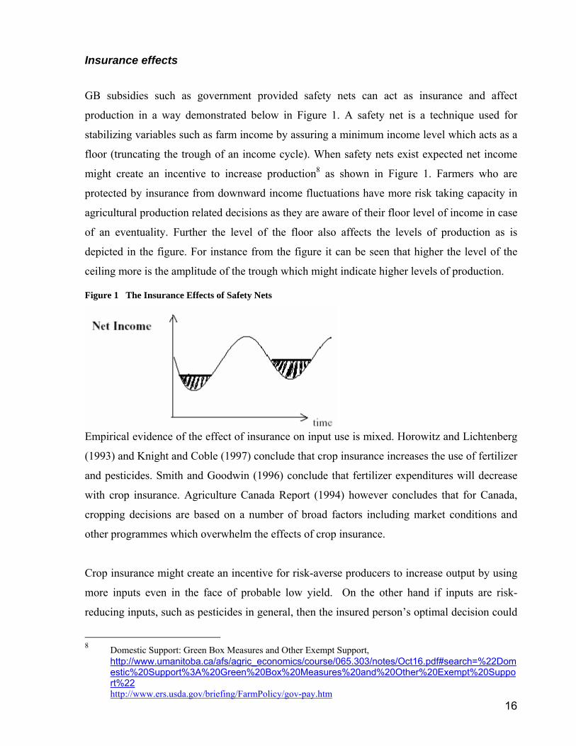
GB subsidies such as government provided safety nets can act as insurance and affect

production in a way demonstrated below in Figure 1. A safety net is a technique used for

stabilizing variables such as farm income by assuring a minimum income level which acts as a

floor (truncating the trough of an income cycle). When safety nets exist expected net income

might create an incentive to increase production8 as shown in Figure 1. Farmers who are

protected by insurance from downward income fluctuations have more risk taking capacity in

agricultural production related decisions as they are aware of their floor level of income in case

of an eventuality. Further the level of the floor also affects the levels of production as is

depicted in the figure. For instance from the figure it can be seen that higher the level of the

ceiling more is the amplitude of the trough which might indicate higher levels of production.

Figure 1 The Insurance Effects of Safety Nets

Empirical evidence of the effect of insurance on input use is mixed. Horowitz and Lichtenberg

(1993) and Knight and Coble (1997) conclude that crop insurance increases the use of fertilizer

and pesticides. Smith and Goodwin (1996) conclude that fertilizer expenditures will decrease

with crop insurance. Agriculture Canada Report (1994) however concludes that for Canada,

cropping decisions are based on a number of broad factors including market conditions and

other programmes which overwhelm the effects of crop insurance.

Crop insurance might create an incentive for risk-averse producers to increase output by using

more inputs even in the face of probable low yield. On the other hand if inputs are risk-

reducing inputs, such as pesticides in general, then the insured person’s optimal decision could

8 Domestic Support: Green Box Measures and Other Exempt Support,

http://www.umanitoba.ca/afs/agric_economics/course/065.303/notes/Oct16.pdf#search=%22Domestic%20Support%3A%20Green%20Box%20Measures%20and%20Other%20Exempt%20Support%22 http://www.ers.usda.gov/briefing/FarmPolicy/gov-pay.htm

17

change as a result of being insured and the producer could be inclined to use less of the input.

In other words, because the insurance contract reduces the loss associated with the insured

event, the producer might be willing to take a more risky decision. This is termed as ‘moral

hazard in crop insurance’ and theoretical models in this area support the conclusion that the

direction of the moral hazard effect on input use, output, and expected indemnities is

ambiguous unless strong assumptions are made about risk preferences and input risk

properties.

Crop insurance also may encourage producers to move risky marginal land into production and

the crop mix may be biased towards production of more risky crops. Agricultural incomes

being subject to instabilities and fluctuations, risk-averse farmers may benefit considerably

from income stabilization measures such as countercyclical subsidies. These income-

stabilization programmes and fixed payments may have a risk-reducing effect.

Cost, price and expectation effects

There are situations where the direct payment can indirectly affect the decisions of risk neutral

producers as well. Such payments help producers to overcome their credit constraints.

Consider a producer who faces a constrained optimization problem. A direct payment may

reduce the constraints limiting this farmer’s production potential and as a consequence leading

him to increase production. Theory suggests that greater the resources available at farmer’s

disposal (Cost outlay) further the isocost line will be from the origin (since more of both labour

(L) and capital (K) can be purchased provided their prices remain the same). This argument

can be even extended to farmers facing no resource constraints as additional resources obtained

through direct payments might be used for purchasing additional inputs. Figure 2 demonstrates

how the producer’s equilibrium shifts from the first isoquant IS0 to another isoquant IS1 at a

higher level of output because the isocost line shifts upward with expanded resources due to

decoupled support (assuming factor prices remain constant).

Figure 2 Shift in Producer’s Equilibrium.

18

There are other potential effects on production such as increases in production executed in

anticipation that the higher level of production now will form the new base for a new

programme (expectation effect). For instance the 2002 Farm Security and Rural Investment

Act in the US aallowed farmers to update their base acres from the 1981-85 planting history

used in the FAIR Act(1996) to a more recent (1998-2001) production history (Amber

Waves,2003).Such base updating might alter producers' expectations of future changes in

program eligibility criteria, which may influence current planting decisions . Even if the

subsidy does not affect marginal production decisions it can affect the decisions to exit or

enter.9

There are a number of examples cited by Rude (1998) on how production might be affected by

GB payments, the first of which is placed in an increasing returns to scale scenario. Increasing

returns imply that at each level of output, marginal cost is less then average cost. In this case a

fixed direct payment would increase average revenue, lowering average cost and increasing

level of production. The second instance where payments based on past performance could

affect current decisions is in the context of behavioural theories of the firm. Instead of

assuming profit maximizing behaviour by the firms these theories assume ‘satisficing’

behaviour. Under satisficing behaviour theory, the interaction of goals through the bargaining

and coalition making process of the organization is assumed to determine resource allocation.

This allocation within the firm reflects only gross comparisons of the marginal advantages of

alternatives. Any alternative that satisfies the constraints and secures suitably powerful support

within the organization is likely to be adopted (Cyert and March;1963). In this context direct

payments loosen constraints and encourage continuation of the status quo, possibly increasing

production. 9 ‘Domestic Support: Green Box Measures and Other Exempt Support’ http://www.ers.usda.gov/briefing/FarmPolicy/gov-pay.htm

19

The third instance cites situations where the producer faces debt constraints. The payment

which was neutral in the non-debt constrained case leads to increased future production in the

debt constrained case (Phimister 1995). Furthermore, Roberts (1997) argues that given a

farmer’s specialized skills, and the absence of perfect capital and information markets,

significant amounts of the fixed direct payments are likely to be invested in the farm even if

there are no debt constraints. There may be more examples of situations in which a direct

payment would relax a production constraint and consequently lead to increased production.

Productivity Effects GB measures could also have a distorting effect on production through increasing productivity.

For instance measures such as research and extension services, conservation, environmental

and natural resource programmes, structural programmes to adjust farm size and numbers,

infrastructure under GB may have production effects on long-term agricultural production.

These programmes cause productivity improvements which shift the supply curve as shown in

Figure 3 increasing output from q0 to q1. If the GB provider is not a small country then, world

prices of agriculture products can decline with possible augmentation of global production.

Figure 3 showcases the mechanism by which world prices go down from P0 to P1 due to the

provision of GB subsidies.

20

Figure 3 Productivity Improvement & Shift in Supply Curve.

GB measures such as environmental programmes might also have impacts on productivity

though this would depend on the nature of the programme and also on the technical relation

between agricultural and environmental factors (Diakosavvas; 2003).

Conclusion

The criteria specified in Annex 2 on classifying GB subsidies try to ensure they are decoupled

from production and hence have no or minimal trade and production distorting effects. But a

review of the literature shows that this may not necessarily be correct as they may influence the

risk behaviour of the producer, have an impact on productivity increases or reduce the cost of

production. These issues have been analysed empirically in the subsequent chapters.

21

II. ANALYSIS OF GB MEASURES OF THE UNITED STATES, EUROPEAN UNION AND JAPAN

As a result of the URAA mandate to reduce trade distorting subsidies it has been argued that

many WTO members have gradually shifted their agricultural support to GB categories

through a readjustment of their domestic policies (Hart and Babcock, 2002). Among the WTO

members the highest level of GB expenditure is by three countries- the US, EU and Japan10. In

2001 the US expenditure on GB policies was $ 50,672 million. This was the highest

expenditure on GB by a member state of the WTO. The GB expenditure by Japan and EU were

also quite high in this period at levels of $ 21,050 million and $ 23,316 million respectively11.

This is in stark contrast to the low levels of GB expenditure by most developing countries. In

this context, an understanding of the structure of domestic support in US, EU and Japan is

essential for any meaningful analysis of the distorting efforts of GB on production and trade.

Hence this chapter examines the structure of domestic support in these three countries both in

terms of the different boxes such as Amber, Blue and Green and also in terms of the various

categories within GB. The objectives of this exercise are threefold. These are to examine

whether in the context of the farm acts enacted in these countries over the past years: (1) there

has been a shift of subsidies between the different boxes among these countries (2) there has

been an increase in GB expenditure in these countries and (3) there has been a greater increase

in some components of GB subsidies compared to others.

Overall Structure of Domestic Support for the US, EU and Japan Table 1 gives the composition of domestic support for the US, EU and Japan across Green

Box, Blue Box and Amber Box. It can be seen that in the US, GB accounted for 74.68 per cent

of the total support spending in 1999. It remained relatively unchanged for 2000, but increased

to 77.85 per cent in 2001 , while amber box expenditure reduced to 22.14 per cent from 25.13

per cent in 2000. GB expenditure in the EU rose from 20 per cent of overall domestic support

in 1995 to about 25 per cent in 2001, while during the same period Amber Box expenditure

reduced from 52 per cent of overall support in 1999 to 47 per cent in 2001. Thus it can be seen

that the pattern of GB support in the EU is similar to that of the US. Japan also shows an

increase in GB expenditure from 47 per cent in 1995 to 77 per cent in 2001 and Amber Box

expenditure reducing from 21 per cent in 1999 to 20 per cent in 2001. Comparing across the

10 This can be inferred from table 12 in chapter 3 which provides the average GB expenditure for the three countries over the period 1995-2000. 11 WTO notifications of EC, US and Japan concerning domestic support commitments.

22

three WTO members, it can be seen that US and Japan have much higher shares of GB support

as a share of their overall domestic support. But all the three members show similar trends in

terms of reduction of amber box spending and increase in their share of GB spending over the

years 1999–2001.In absolute levels the increase in GB might not be very large or might have

even showed small declines. But the fact to be noted is that while the other categories of

domestic support such as Blue box and Amber box have declined, there has been no such

proportional decline in GB. This might indicate the probability of box shifting.

Table 1 Structure of Domestic Support for the US, EU and Japan (in Domestic Currencies). United States (Million US Dollars) 1995 1998 1999 2000 2001 amount % of Total

Domestic Support

amount % of Total Domestic Support



amount %DSu

Green box

46,033 88 49,824

83%

49,794

74%

50,057

74%

50,672

77

Blue box

0 0 0 0 0 0 0 0

Total AMS

6213 12 10,391 17% 16,862.2 25 16,802.58 25 14,413.05 2

others

0 0 0 0 0 0 0 0 0

Total

52,246

60,215 100 66,611 100 66,860 100 65,085 10

European Union (Million Euro) 1995 1998 1999 2000 2001 % of

Total Domestic Support

Amount % of Total Domestic Support



Amount %DSu

Green Box 18,718.00 20% 19,168 22% 19,930.50 23% 21,844.50 25% 20,661.20Total AMS 47,526.40 52% 46,683 54% 47,885.70 55% 43,654 50% 39,281.30Blue Box 25412.3061 28% 20503.5 24% 19,792.10 23% 22,222.70 25% 23,725.90Total 91,656.71 86,355 87,608.30 87,721.20 83,668.40 Japan (Billion Yen) 1995 1998 1999 2000 2001 % of

Total Domestic Support




Amount DSu

Green Box 3169 47% 3001.6 79% 2685.9 76% 2595.3 76% 2546.9Blue Box 3,507.50 53% 766.5 20% 747.8 21% 708.5 21% 666.7Total AMS 0 0% 50.2 1% 92.7 3% 92.7 3% 91.1Total 6,676.50 3818.3 3526.4 3396.5 3304.7 Source- WTO Notifications

23

Box 1 Box Shifting.

The pattern of domestic support in the US, EU and Japan has changed significantly over the past few years, with the proportion of GB component increasing in the total domestic support, commonly referred to as box shifting. The US has increased its GB spending by a large amount over the past several years. Over the period 1986–88, programmes that would have qualified for the GB had total expenditures of, on average, just over $26 billion. From 1996 to 1998, GB spending had increased to an average of $50 billion( Hart and Babcock ,2002). Because the GB spending is exempt from WTO limits, the US can continue to add to this total. In the EU and Japan, the phenomenon is more recent: from 1995 onwards, Amber and Blue Box expenditures have reduced, while GB spending has increased or remained at similar levels. In the EU, GB as a percentage of total domestic support has increased from 21 per cent in 1995 to 25 per cent in 2001. In Japan, the GB percentage increased from 46 per cent in 1995 to 78 per cent in 2000. It has been estimated that as a result of the CAP 2003 reforms, the EU would be in a position to shift about 75 per cent of its subsidies from the Blue Box to the GB ( Agra Europe ,2003). Further, the GB subsidies might remain partially coupled to the present or future production, leading to distortions in production. The partial coupling could occur because of two factors. (1) The fact that the US and EU Acts have not defined an unchanging base period could lead to expectation effects that might lead to an increase in production (2) Further exclusion of direct payments to certain crops such as fruits and vegetables under both the Production Flexibility Contracts (PFCs) in the US and also under the CAP reforms in the EU could lead to a distortion in the production structure. Supporting these theoretical arguments, certain assessments conducted for the EU find that decoupled payments would increase the production of most of the cereals in 2009 compared to 2002. To conclude, the likely shift in certain developed countries towards providing support through the GB would be a cause of concern; particularly because the decoupling is only partial and even decoupled subsidies can be production and trade distorting( Agra Europe ,2003).

Box 2 Farm Reforms in the United States.

Fair Act (Federal Agricultural Improvement & Reform Act) 1996 introduced production flexibility contracts or PFCs which ran from 1996 to 2002. These payments were based on past production and were independent of current market prices and farmers’ planting decisions. These fixed payments replaced the earlier deficiency payments but did not require continued production of the crop for which payments were received. A mechanism was also put in place for many crops that allowed farmers to receive a cash payment—a ‘marketing gain’ or ‘loan deficiency payment’ (LDP) — if market prices were below their loan rate levels. Farm Act 2002 replaced PFCs by a very similar scheme of direct payments which were extended to cover more crops such as soybeans, other oilseeds, and peanuts. Fixed direct payments are not tied to production of specific crops, the amount of production, or the price of the crop. This bill also introduced counter cyclical support payments. This program was developed to provide an improved counter-cyclical income safety net to replace most ad hoc market loss assistance payments that were provided to farmers during 1998-2001. Payments are based on historical production and are not tied to current production. This bill also retained the marketing assistance provisions from 1996 and extended it further to peanuts, wool, mohair, and honey. To support dairy farmers a new market loss payments programme was developed to provide a price safety net and to replace ad hoc market loss assistance payments that were provided to milk producers in 1999, 2000, and 2001. It has been argued that the PFCs provided under the Act of 1996 and the direct payments under the Act of 2002 are not totally decoupled and might have production distortion effects. Given the limited data availability, production estimates are difficult to make. However, evidence from the US on PFCs suggests that these subsidies have increased the total planted acreage. The Economic Research Service (ERS) predicts that under the PFCs the area of total plantings increased by between 225,000 to 725,000 acres. Further under the 1996 Farm Act the PFC payment scheme excluded fruits and vegetables. The provisions under the payment scheme which replaced the 2002 Farm Act are the same except for the fact that wild rice would also be treated the same as a fruit/vegetable. This exclusion is criticized for its distorting effect on the production decisions of producers in the US. The Acts have also been criticized on the basis that

24

not defining an unchanging base period might create expectation effects among producers that would lead to an increase in the production.

Category wise Expenditure on GB by the US, EU and Japan

This section examines the spending of US, EU and Japan under the different GB categories—

General Services, Public Stockholding for Food Security Purposes, Domestic Food Aid,

Decoupled Income Support, Income Insurance and Income Safety Net Programmes, Payments

for Relief From Natural Disaster, Structural Adjustment through Producer/Resource

Retirement Aids, Structural Adjustment through Investment Aids, Environmental Programme

Payments, Regional Assistance Programmes.

General Services GB policies on general services involve expenditures in relation to programmes which provide

services or benefits to agriculture or the rural community. They do not include direct payments

to producers or processors. General services apart from meeting the general criteria also

include categories such as general research, pest and disease control, training services,

extension and advisory services, inspection services, marketing and promotion services and

infrastructural services.

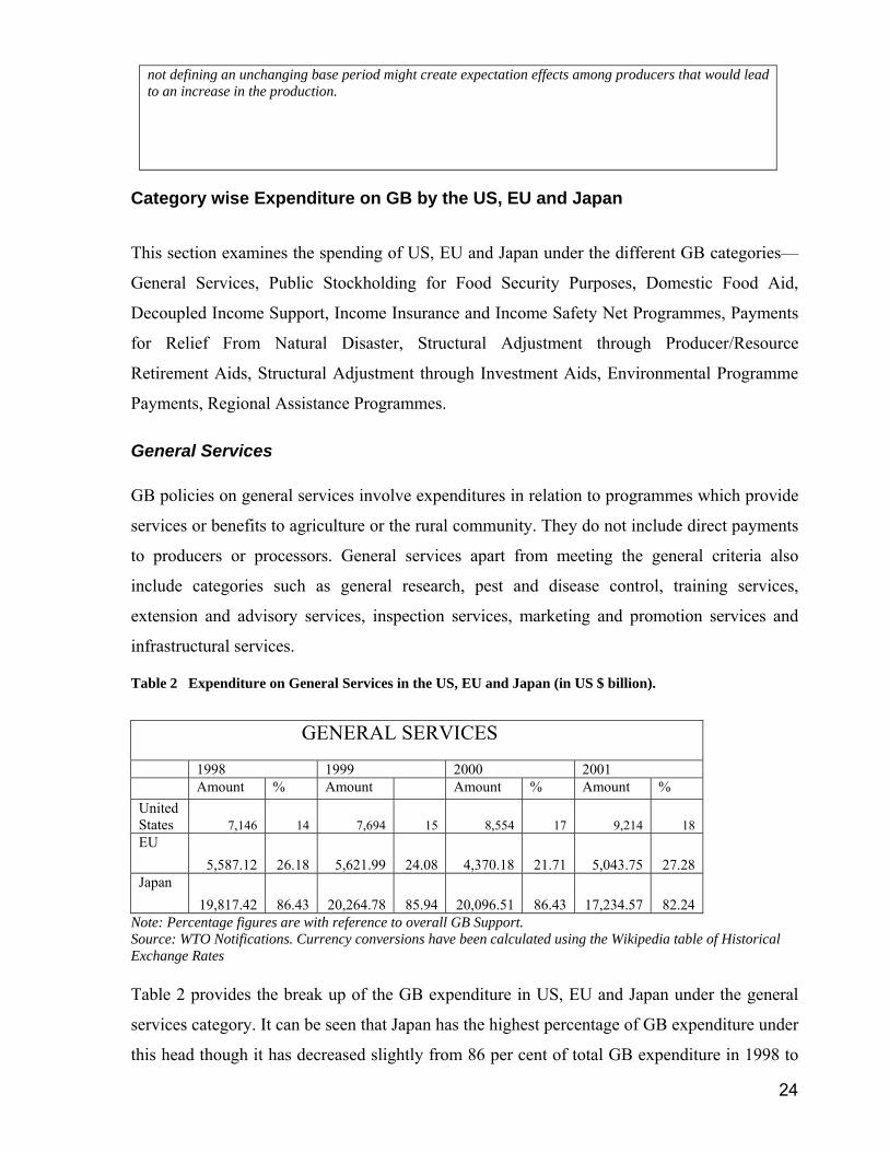
Table 2 Expenditure on General Services in the US, EU and Japan (in US $ billion).

GENERAL SERVICES

1998 1999 2000 2001 Amount % Amount Amount % Amount % United States 7,146 14 7,694 15 8,554 17 9,214 18 EU

5,587.12 26.18 5,621.99 24.08 4,370.18 21.71 5,043.75 27.28 Japan

19,817.42 86.43 20,264.78 85.94 20,096.51 86.43 17,234.57 82.24 Note: Percentage figures are with reference to overall GB Support. Source: WTO Notifications. Currency conversions have been calculated using the Wikipedia table of Historical Exchange Rates Table 2 provides the break up of the GB expenditure in US, EU and Japan under the general

services category. It can be seen that Japan has the highest percentage of GB expenditure under

this head though it has decreased slightly from 86 per cent of total GB expenditure in 1998 to

25

82.24 per cent of GB expenditure in 2001. EU’s expenditure under this head has been stable

over the period 1998–2001 at around 26 per cent. The US expenditure in General services

category has been much lower compared to EU and Japan and constitutes only 18 per cent of

overall GB support in 2001, though there has been a slight increase from 14 per cent in 1998 to

18 per cent in 2001. Theoretically expenditure on general services is argued to distort trade and

production by increasing productivity of agricultural production. For instance as depicted in

Figure 3 (Chapter 1) GB expenditure under general services might shift the agricultural

products supply curve with an increase in productivity. This theoretical argument is also

supported by our empirical analysis. For instance our DEA analysis in the next chapter shows

that Japan experiences the highest Total Factor Productivity increase as a result of GB

expenditure. The reason for this may lie in the fact that majority of Japan’s GB expenditure is

in the form of General Services.

Public Stockholding for Food Security Purposes

GB support in this category includes expenditure towards the accumulation and holding of

stocks of products which form an integral part of a food security programme identified in

national legislation. The volume and accumulation of such stocks correspond to predetermined

targets related solely to food security.

Table 3 Expenditure on Public Stockholding for Food Security Purposes in the US, EU and Japan (in US $ million)

Public Stockholding for Food Security Purposes

1998 1999 2000 2001 Amount % Amount Amount % Amount % United States 0 0 0 0 0 0 0 0 EU

21.26 0.100 21.30 0.091 17.87 0.089 16.19 0.088 Japan

432.37 1.89 410.86 1.74 430.57 1.85 356.29 1.70 Note: Percentage figures are with reference to overall GB Support Source: WTO Notifications. Currency conversions have been calculated using the Wikipedia Table of Historical Exchange Rates Table 3 provides the GB expenditure of US, EU and Japan under the public stockholding for

food security purposes category. It can be seen that US does not have any spending under this

category. Japan has been spending around 1.9 per cent of its overall GB on public

26

stockholding. The EU has been spending even less and from 1998 to 2001 the overall spending

by EU on this category has fallen from 1 per cent to .088 per cent of total GB expenditure.

Domestic Food Aid

Domestic food aid under GB involves expenditures on food aid to sections of the domestic

population in need. Clearly defined criteria related to nutritional objectives determine the

eligibility to receive food aid. Though food aid might not have any directly distorting effects

on the cost of production it might have minor impacts on production. In fact a 2002 ERS

report12 using CGE modelling found that cuts in the US food programme could marginally

decrease farm and food processing production.

Table 4 Expenditure on Domestic Food Aid in the US, EU and Japan (in US $ million)

Domestic Food Aid

1998 1999 2000 2001 Amount per

cent Amount Amount per

cent Amount per

cent United States 33,487 67 33,050 66 32,377 65 33,916 67 EU

306.98 1.44 295.97 1.27 248.94 1.24 217.27 1.18 Japan

105.42 0.46 81.65 0.34 50 0.21 4 0.20 Note: Percentage figures are with reference to overall GB Support. Source: WTO Notifications Currency conversions have been calculated using the Wikipedia Table of Historical Exchange Rates The above table depicts the expenditure of US, EU and Japan on domestic food aid. US spends

the largest proportion of its overall GB expenditure on domestic food aid. EU and Japan spend

a very small percentage of their overall GB expenditure on this category with that of EU

declining from 1.44 per cent in 98 to 1.18 per cent in 2001 and that of Japan declining from

0.46 per cent to 0.20 per cent in 2001.

Decoupled Income Support Direct payments to producers are considered decoupled payments if they are not related to or

based on market prices (domestic and international), the type or volume of production, or

factors of production in any year after a defined and fixed base period. Decoupled income 12 Tracing the Impacts of Food Assistance Programs on Agriculture and Consumers: A Computable General Equilibrium Model http://www.ers.usda.gov/Publications/fanrr18/

27

support arguably reduces the cost of production as depicted in figure 2 displayed earlier. This

would have distortive effects on production and trade . Such payments might also have a

wealth effect, and hence significant effects on acreage decisions of different crops. Decoupled

payments can cover fixed and variable production costs, help overcome capital constraints by

influencing supply of loans to producers, affect expectations, and retain producers in

agriculture where exiting would be the rational decision( Abler and Blandford ,2005).

Table 5 Expenditure on Decoupled Income Support in US, EU and Japan (in US$ million).

Decoupled Income Support 1998 1999 2000 2001 Amount per


cent Amount Per

cent US 5,659 11 5,471 11 5,068 10 4,100 8 EU 143.19 0.67 1020.14 4.37 454.49 2.26 148.46 0.80 Japan 0 0 0 0 0 0 0 0

Note: Percentage figures are with reference to overall GB Support Source: WTO Notifications. Currency conversions have been calculated using the Wikipedia Table of Historical Exchange Rates On comparing decoupled income support in EU, US and Japan it can be seen that the

decoupled support provided by the US has fallen over the years from 11 per cent of overall GB

expenditure to 8 per cent. In the EU decoupled income support increased from 98 to 99 from

0.67 per cent of overall GB to 4.37 per cent but thereafter decreased to 0.80 per cent in 2001.

Japan did not notify any decoupled income support during this period. Though there has been a

decline in decoupled income support within the US, it still has the highest expenditure on this

category among these three countries. Under the 2002 Farm Bill decoupled direct payments are

the highest for wheat and corn ($ 0.52 and $ 0.28 per bushel)13 after rice and peanuts. This

might be the reason why our subsequent empirical analysis of the Cobb Douglas Cost function

shows the maximum impact of decoupled payments on wheat and corn.

Box 3 Farm Reforms in the European Union.

Common Agricultural Policy (CAP) Reforms 1993–5 CAP Reforms introduced direct payments and strengthened environmental efforts. 2000 CAP Reforms The stated objective of these reforms was to decrease government interventions, price and subsidy support while increasing compensation and direct income support payments. This reform also allowed Member countries to offer direct payments to environmental programmes and provided financial support to environment-friendly activities such as organic farming and protecting semi-natural residential areas, wetlands and traditional orchards. 2003 CAP Reforms The main feature of this reform was the introduction of a single payment scheme for the EU farmers, decoupled from production with limited ‘coupled’ elements where member states consider

13 http://www.farmfoundation.org/projects/documents/Westcott_000.pdf

28

this necessary to avoid abandonment of production, and the requirement for cross compliance which entails that the single payment be linked with environmental, food safety, animal and plant health and animal welfare standards, as well as to the requirement to keep all farmland in good agricultural and environmental condition. This act has been criticized on the basis that the decoupled payments might have impacts on production. Further the EU proposals on decoupling are even more flexible than the US proposals since they do not require land to be under production but in good ‘agricultural condition’. More importantly, there is a possibility of changing the base period in future which might lead to expectation effects among the producers which would in turn lead to increased agricultural production. Further the single payment scheme under the CAP reforms of 2003 may be used for any agricultural activity except for fruit, vegetables and table potatoes. This exclusion might as in the case of US PFCs lead to distortions in production. In fact certain assessments conducted for the EU find that decoupled payments would increase the production of most of the cereals in 2009 compared to 2002.

Income Insurance and Income Safety Net Programmes Direct payments to producers are considered to be income insurance and safety net payments if

they meet four policy specific criteria:

eligible producers have experienced a loss that exceeds 30 per cent of average gross

income, or the equivalent in the preceding 3–5 years;

the amount of such payments compensates less than 70 per cent of the eligible producer’s

income loss in the year,

payments relate solely to income and not to prices, production or factor use; and

payments from this provision combined with that for natural disaster total to less than 100

per cent of the total loss for individual farmers.

Both US and Japan have not notified any expenditure under this head during 1998–2001. The

EU has notified during the years 2000 and 2001, $ 4.61 and $ 9.57 million respectively.

Table 6 Expenditure on Income Insurance and Income Safety Net Programmes in the US, EU and Japan (In US million Dollars)

Income Insurance and Income Safety Net Programmes

1998 1999 2000 2001 Amount per


cent Amount per

cent United States 0 0 0 0 0 0 0 0 EU

0 0 0 0 4.61 0.02 9.57 0.05 Japan

0 0 0 0 0 0 0 0

29

Note- Percentage figures are with reference to overall Green Box Support Source- WTO Notifications Currency conversions have been calculated using the Wikipedia table of Historical Exchange Rates Both US and Japan have not notified any expenditure under this head during 1998-2001. The

EU has notified during the years 2000 and 2001 4.61 and 9.57 million US dollars respectively.

Payments under income insurance and safety net programmes theoretically can be argued to

have a production and trade distorting effect as is depicted by Figure 1 in Chapter 1.

Payments for Relief from Natural Disaster In terms of distortions in costs of production natural disaster payments might have two

conflicting effects: on the one hand they could help producers cover costs which they would

otherwise incur themselves and on the other hand they might also raise moral hazard issues that

would induce farmers to produce in risky environments. But natural disaster payments also

have an economic justification since they help ameliorate market failures.

Table 7 Expenditure on Payments for Relief from Natural Disaster in US, EU and Japan (in US$ million).

Payments for Relief From Natural Disaster 1998 1999 2000 2001 Amount per


cent Amount per

cent US 1,411 3 1,635 3 2,141 4 1,421 3 EU 203.32 0.95 389.41 1.67 359.87 1.79 356.87 1.93 Japan 447.65 1.95 508.31 2.16 515.01 2.21 445.16 2.12

Note: Percentage figures are with reference to overall GB Support Source: WTO Notifications. Currency conversions have been calculated using the Wikipedia Table of Historical Exchange Rates Over the period 1995–2001 the US has been spending 3 per cent of its overall GB expenditure

on this category of support. The US expenditure on this head has been higher than both the EU

and Japanese expenditure. However, it must be noted that the EU and Japanese expenditure on

this category has increased from 1998 to 2001.

Structural Adjustment through Producer/Resource Retirement Aids The US expenditure on this category has remained stable over the period 1998–2001 at 3 per

cent of overall US expenditure on GB. The percentage of expenditure on structural adjustment

on producer/retirement aids as a percentage of overall GB has declined for the EU from 5.93

30

per cent in 1998 to 4.33 per cent in 2001. As per Japan’s notification the expenditure on this

head has increased slightly from 2.8 per cent in 1998 to 3.85 per cent in 2001.

Table 8 Expenditure on Structural Adjustment through Producer/Resource Retirement Aids in US, EU and Japan (in US$ million).

Structural Adjustment through Producer/Resource Retirement Aids 1998 1999 2000 2001 Amount Per


cent Amount per

cent US 1,731 3 1,434 3 1,476 3 1,624 3 EU 1265.78 5.93 974.96 4.18 692.37 3.44 799.91 4.33 Japan 652.381 2.85 754.124 3.20 824.015 3.54 806.392 3.85

Note: Percentage figures are with reference to overall GB Support Source: WTO Notifications. Currency conversions have been calculated using the Wikipedia Table of Historical Exchange Rates

Structural Adjustment through Investment Aids The EU’s expenditure on structural adjustment through investment aids programme comprised

a significant portion of its overall expenditure on GB though the overall EU share of

expenditure on this head has fallen from 28.18 per cent in 1998 to 25.92 per cent in 2001.

Table 9 Expenditure on Structural Adjustment through Investment Aids in US, EU and Japan (in US$ million)

Structural Adjustment through Investment Aids 1998 1999 2000 2001 Amount per


cent Amount per

cent US 93 0.19 134 0.27 132 0.26 106 0.21 EU 6014.14 28.18 6120.82 26.21 5721.49 28.42 4792.13 25.92 Japan 591.27 2.58 476.70 2.02 476.70 2.02 348.89 1.66


Environmental Programme Payments Direct payments to producers under environmental programmes qualify as GB payments if

they are part of a clearly defined government environmental or conservation programme and

are also dependent on the fulfilment of specific conditions under the government programme

including conditions related to production methods or inputs. The amount of payment under

this is limited to the extra cost or loss of income from complying with such conditions.

31

Table 10 Expenditure on Environmental Programme Payments in US, EU and Japan (in US$ million)

Environmental Programme Payments 1998 1999 2000 2001 Amount per


cent Amount per

cent US 297 0.60 332 0.67 309 0.62 291 0.57 EU 5528.45 25.90 5815.79 24.91 5274.83 26.21 4938.70 26.71 Japan 883.08 3.85 1083.34 4.59 516.87 2.22 1450.68 6.92

Note: Percentage figures are with reference to overall GB Support Source: WTO Notifications. Currency conversions have been calculated using the Wikipedia Table of Historical Exchange Rates Environmental payments comprise a significant portion of the EU’s GB expenditure and have

increased from 25.9 per cent in 1998 to 26.71 per cent in 2001. The US expenditure has not

been very significant under this head. Japan’s environmental payments have increased from 3.8

per cent in 1998 to 6.92 per cent in 2001. Although it is argued that environment subsidies are

hardly production and trade distorting, distortions are indeed possible. For instance GB support

under this head might affect costs through the introduction of more cost reducing

environmentally friendly technologies which might not have been otherwise adopted due to

fixed costs now being covered by the subsidies. Environmental payments might also affect

production decisions in the same manner as general services by increasing productivity.

Regional Assistance Programmes In terms of regional assistance programmes the US has not notified any expenditure in this

category. The EU’s expenditure on such programmes had increased from 10.6 per cent in 1998

to 14.83 per cent in 2000 but thereafter declined to 11.71 per cent in 2001.

Table 11 Expenditure on Regional Assistance Programmes in US, EU and Japan (in US$ million)

Regional Assistance Programmes 1998 1999 2000 2001 Amount per


cent Amount per

cent US 0 0 00 0 0 0 0 0 EU 2272.58 10.65 3089.39 13.23 2984.34 14.83 2165.91 11.71 Japan - - - - 306.22 1.32 271.54 1.30


32

Conclusion

It can be seen that the US has steadily maintained quite a high proportion of GB expenditure

from 1995 onwards. In EU the share of GB expenditure in the overall domestic support has

increased from 1995 onwards. In the case of Japan also it can be seen that there has been an

increase in the share of GB in the overall domestic support from 47% in 1995 to 75% in 2001.

It is further observed that while for US the most significant categories of GB expenditure are

domestic food aid and general services respectively, for EU it is general services followed by

investment aid. In Japan the most significant category of GB expenditure is general services.

Environmental payments also comprise an increasingly important part of GB expenditure in

both the EU and Japan. Over this period there has been a change in farm support policies in

US, EU and Japan which has led to a shift of domestic support to agriculture from Amber Box

measures to GB measures. Further it can be seen that while there has been a decline in the

magnitude of all subsidies provided, the decline in GB has not been proportionate to the

decline in other subsidies and at times there has also been an increase in GB subsidies

compared to other subsidies. This might be an indication of box shifting.

33

III. DEA ANALYSIS AND CGE MODELLING

Earlier in the paper theoretical arguments were advanced to show how GB subsidies might

have an impact on trade and production This chapter examines as explained above the trade

and production effects of GB using Data Envelopment Analysis (DEA) and CGE modelling.

DEA is a widely used technique for estimating the impact of subsidies on output. DEA allows

comparison of total factor productivity (TFP) across countries with and without subsidies. With

DEA analysis it is possible to compare the sources of productivity improvements across

countries It not only provides comparable percentage changes in productivity but also

decomposes TFP into technical change and technical efficiency. Productivity enhancement

leads to reduction in cost of production thus resulting in an improvement in cost efficiency.

Therefore DEA is also used to estimate cost efficiencies across countries. To translate the

results of DEA into effects on production and trade, CGE modelling is used. An improvement

in total factor productivity and a corresponding rise in cost efficiency can result in changes in

the pattern of global production and trade.These changes are quantified through CGE

modelling. This is a comprehensive methodology for taking account of simultaneous changes

across countries.

Data Envelopment Analysis (DEA) Estimation DEA is a linear-programming methodology, which uses data on the input and output quantities

of a group of countries to construct a piece-wise linear surface over the data points. A frontier

surface is then constructed by the solution of a sequence of linear programming problems—one

for each country in the sample. The degree of technical change of each country (the distance

between the observed data point and the frontier) arrived at is a by-product of the frontier

construction method.

DEA can be either input-oriented or output-oriented. In the input-oriented analysis, the DEA

method defines the frontier by seeking the maximum possible proportional reduction in input

usage, with output levels held constant, for each country. In the output-oriented analysis, the

DEA method seeks the maximum proportional increase in output production, with input levels

held fixed. The two measures provide the same technical efficiency scores when a constant

returns to scale (CRS) technology applies, but are unequal when variable returns to scale

(VRS) are assumed14. This paper assumes VRS technology and selects the output oriented

14 Agricultural production is generally assumed to have variable returns to scale

34

approach for calculating production efficiency since it is fair to assume that, in agriculture, one

usually attempts to maximize output from a given set of inputs, rather than the converse15. For

calculating cost efficiencies, however, this paper uses an input oriented approach.

The DEA analysis may be divided into three parts. First, total factor productivity growth for 25

countries for the period 1995–2000 is estimated using Malmquist indices16, which are defined

by distance functions. One output and three inputs (land, labour and capital) are used to

construct these indices. This constitutes a base line frontier. Second, the same exercise is

undertaken with GB expenditure as an additional input. Total factor productivity growth is

further decomposed into technical efficiency (TE) growth and technical change (TECHCH),

which is represented by a shift in the production frontier. However, since the two TFP

estimates have been obtained using two different frontiers, the relative distances from the

frontier are estimated for each country. The difference in the relative TFP scores gives the

change in TFP on account of GB expenditure. Third, cost efficiency (CE) is estimated for the

year 2000 with and without GB expenditures. Here domestic food aid, public stock holding for

food security purposes and relief from natural disaster components are removed from total GB

expenditure to arrive at the adjusted GB expenditures.17 The relative improvement in cost

efficiency for each country is estimated, as in the earlier case, by calculating the change in its

relative distance from the frontiers. Using this, the change in cost efficiency due to GB

expenditures is estimated through an input oriented approach. These changes are then used as

shock variables in the CGE modelling to determine output and trade changes in different

countries.

15 This has also been argued by Tim Coelli and Prasada Rao (2003). 16 Explained further in Appendix 1 17 Public stockholding for food security purposes and Natural disaster relief payments have an economic justification since they ameliorate market failures .The effect of food aid component on cost of production is found to be insignificant in the subsequent Cobb Douglas Estimate. Hence this paper removes these three categories of GB from the DEA and CGE analysis.

35

Malmquist TFP Indices As a first step Malmquist indices are calculated. Malmquist indices help reaffirm the

robustness of the results obtained from the estimation of cost efficiencies. To estimate the

change in TFP, TE and TECHCH, with and without GB expenditures, the countries are

categorized as high GB, medium GB and low GB spending in the period 1995–2000. US,

Japan and EU are categorized as countries with high GB expenditures. These are reported in

Table 12 below.

Table 12 Average GB Expenditure (US$ million) 1995–2000. High GB United States 50277 Japan 25077 EU 23953Medium GB Korea, Rep. 4972 Brazil 3238 Switzerland 2331 India 2196 Mexico 1508 Thailand 1248 Canada 1178Low GB Australia 787 Poland 677 Venezuela, RB 598 Norway 567 South Africa 557 Pakistan 359 Morocco 279 Philippines 264 Colombia 253 Indonesia 248 Argentina 231 Malaysia 217 Czech Republic 170 Peru 143 Chile 140 New Zealand 128 Sri Lanka 108

Trinidad and Tobago 63

Tunisia 43 Iceland 42 Paraguay 38 Costa Rica 32 GB expenditures of US, EU and Japan are more than six times that of medium GB countries.

36

Estimation of TFP Changes

The average TFP, TE and TECHCH scores estimated with Malmquist indices for 25 countries

for the period 1995–2000 are reported in Table 1318. The analysis uses agricultural arable land,

agricultural labour and number of tractors as inputs, where the data are collected from World

Development Indicators (2006). GB expenditure is used an one of the inputs in the calculation

of these scores. The estimates show that maximum TFP growth in this period has occurred in

US (9.6 per cent) followed by Japan (6.2 per cent) and Brazil (5.9 per cent). EU has also

witnessed TFP growth of 2.0 per cent. Interestingly, in countries with very high GB, that is,

U.S, EU and Japan, it is found that most of the growth in TFP is explained by technical change

rather than improvement in technical efficiency. The negative impact of subsidies on technical

efficiency in agriculture is also supported by empirical studies like Rezitis et al (2003) and

Giannakas et al (2001) for Greece and Canada respectively which show that subsidies may

reduce incentives for efficiency improvements.

On the other hand, there was a drastic technical change for US in this period. EU and Japan

also experienced positive technical change of 1.8 per cent and 5.5 per cent respectively. A rise

in Research and Development expenditures may have shifted the production frontier outwards.

Making expensive technologies available at a lower price could also have enabled farmers to

produce more. Similar effects of subsidy on technical change in agriculture have been found by

Guyomard et al (2006) for France in the period 1995 to 2002 using a comparable methodology.

Table 13 Mean of Total Factor productivity, Technical Efficiency and Technical Change with GB Expenditures (Malmquist Indices).

S. No. Country Technical

Efficiency Change

Technical Change

Pure Efficiency Change

Scale Efficiency Change

Total Factor Productivity Change

1 High GB EU 1.002 1.018 0.979 1.024 1.020 2 High GB Japan 1.006 1.055 1.000 1.006 1.062 3 High GB United States 1.000 1.096 1.000 1.000 1.096 4 Medium GB Brazil 1.019 1.039 1.000 1.019 1.059 5 Medium GB Canada 1.000 1.027 1.000 1.000 1.027 6 Medium GB India 0.987 1.000 0.945 1.044 0.987 7 Medium GB Korea, Rep. 1.000 1.001 1.000 1.000 1.001 8 Medium GB Mexico 0.984 1.031 0.950 1.034 1.015 9 Medium GB Poland 0.914 1.067 0.856 1.068 0.975

10 Medium GB Switzerland 0.980 1.036 0.998 0.982 1.015 11 Medium GB Thailand 0.959 1.056 0.991 0.969 1.013

18 All indices are relative to the previous year. For each of the indices 1.000 indicates no change.For eg a Total Factor Productivity Index of 1.000 indicates no change and an index of 1.059 indicates a change of 5.9%.

37

12 Low GB Argentina 1.016 1.000 1.000 1.016 1.016 13 Low GB Australia 1.000 1.048 1.000 1.000 1.048 14 Low GB Chile 0.907 1.000 0.918 0.989 0.097

15 Low GB Czech

Republic 1.016 0.984 1.000 1.016 1.000 16 Low GB Indonesia 0.955 0.987 0.939 1.017 0.942 17 Low GB Malaysia 1.049 1.000 1.000 1.049 1.049 18 Low GB Morocco 1.000 0.983 1.000 1.000 0.983 19 Low GB Norway 0.984 1.034 1.000 0.984 1.017 20 Low GB Pakistan 1.005 1.000 1.000 1.005 1.005 21 Low GB Peru 1.003 1.000 1.003 1.000 1.003 22 Low GB Philippines 1.020 1.000 1.000 1.020 1.020 23 Low GB South Africa 1.092 1.035 1.094 0.998 1.130 24 Low GB Sri Lanka 1.015 1.000 1.000 1.015 1.015 25 Low GB Venezuela, RB 1.020 1.020 1.010 1.010 1.040

Note: A value of 1.00 indicates the there has been no change in the variable. Indices higher than 1.00 indicate percentage increase of that magnitude. Upon decomposing the TFP it is found that for most of the low GB countries, except for South

Africa, no significant technical change has occurred in this period.

To estimate the impact of GB expenditures on TFP, TE and TECHCH for each country the

difference in TFP with the frontier country is estimated. The difference in the relative

distances gives the change due to GB expenditures in TFP, TE and TECHCH. The results are

reported in Table 14.

Table 14 Change in TFP, Technical Change and Change in TE due to GB Expenditures (per cent): 1995 to 2000.

S.No Extent of

GB Country Name Change in TFP

due to GB Change in TECH due to GB

Change in TE due to GB

1 High GB EU 2.0 1 -2.5 2 High GB Japan 4.2 2.6 -4.6 3 High GB United States 2.9 2.2 -1.5 4 Medium GB Brazil 2.0 3.6 -0.1 5 Medium GB Canada -3.0 -0.1 -1.5 6 Medium GB India -0.3 -2.8 0.1 7 Medium GB Korea, Rep. 1.8 2.8 -1.5 8 Medium GB Mexico 1.3 1.2 1.5 9 Medium GB Poland -1.2 1.9 -1.6

10 Medium GB Switzerland 3.0 2.1 -1.1 11 Medium GB Thailand 0.5 1.6 -1.4 12 Low GB Argentina -1.8 -1 -1.3 13 Low GB Australia -1.6 -1.6 -0.5 14 Low GB Chile -5.9 0.7 -0.8 15 Low GB Czech Republic -3.1 -4.3 0.2 16 Low GB Indonesia -5.8 -4.1 0.1 17 Low GB Morocco -2.5 -4.6 1.5 18 Low GB Norway -0.2 -1.1 -2.5

38

19 Low GB Pakistan -4.1 -1.6 0.1 20 Low GB Peru -0.3 -5.7 2.8 21 Low GB Philippines 1.2 -4.8 3.7 22 Low GB South Africa 1.8 3.5 0.6 23 Low GB Sri Lanka -0.2 -0.3 1.6 24 Low GB Venezuela, RB -1 1.6 1.5

The results show that there has been an increase in TFP on account of GB expenditures in all

three high GB countries. Japan has experienced the highest increase of 4.2 per cent.

Productivity growth has declined relative to the frontier in most of the developing countries,

especially the ones with low GB expenditures as US defines the frontier. Korea, Switzerland

and Thailand, which are medium GB expenditure countries, experience a rise in their

productivity with GB expenditures.

GB expenditures account for 2.2 per cent of technical change in US. For medium GB

countries, such as Thailand, Mexico, Korea and Switzerland it leads to improvement in relative

positions with respect to technical change, while those of low GB countries worsen. Technical

efficiency, on the other hand, improves in countries with low GB expenditures but declines for

the high GB countries. Similar results with respect to technical efficiency (that is, no change in

TE in US and a decline in technical efficiency in Japan) have also been found by Coelli and

Rao (2003) who estimate Malmquist indices for US agriculture for the period 1980 to 2000.

Guyomard et al (2006) also find that CAP direct payments expressed as a share of farm

revenue in France in the period 1995 to 2002 had a negative impact on technical efficiency. GB

subsidy may therefore reduce incentives for improving efficiency, though over time these

payments may help the farmers to get closer to their frontier due to significant enhancement of

productivity growth.

Estimation of Cost Efficiencies Deterministic DEA

To translate the impact of productivity changes with and without GB expenditures on output

and trade to cost efficiency changes, cost efficiencies are estimated using input-oriented DEA

approach. A similar methodology is followed whereby two cost frontiers are estimated, with

and without GB expenditures. For a particular country, change in relative distance from the

two frontiers is arrived at. The difference between the two distances gives the change in cost

efficiency of the country which can be attributed to GB expenditures.

39

Availability of cost data is limited; cost efficiencies have been estimated for the year 2000 for

select countries where comprehensive data is available. Adjusted GB expenditure excluding

subsidies for public stock holding, domestic food aid, relief from natural disasters and others is

used for our purposes because it is expected that these categories may not affect cost of

production, Notifications for the latest available years are used to disaggregate GB

expenditures. The adjusted GB expenditures are reported in Table 15.

Table 15 Decomposition of GB Expenditures in US Million Dollars (For the year 2000).

Serial

no. Extent of GB Country Unadjusted

GB Adjusted GB Food Aid

Component ( per cent)

1 High GB EU 20,125.76 19,516.40 3.02 High GB Japan 24081.841 23,081.00 4.23 High GB United States 50,057.00 15,540.00 69.04 Medium GB Brazil 1,486.00 856.00 42.45 Medium GB Canada 1,594.49 1,594.49 0.06 Medium GB India 2,872.85 411.25 85.77 Medium GB Korea, Rep. 4468.7 4271 4.48 Medium GB Mexico 508.21 508.21 0.09 Medium GB Poland 557 490.12 12.010 Medium GB Switzerland 2031.57 2026.06 0.311 Medium GB Thailand 977.53 977.53 0.012 Low GB Argentina 156.23 156.23 0.013 Low GB Australia 752.17 729.85 3.014 Low GB Chile 108.85 108.85 0.015 Low GB Czech Republic 171.82 139.99 18.516 Low GB Indonesia 507.18 125.40 75.317 Low GB Malaysia 130.21 130.21 0.018 Low GB Morocco 250.424 61.64 75.419 Low GB Norway 569.384 536.15 5.8420 Low GB Pakistan 238.42 230.24 3.421 Low GB Peru 279.7 223.4 20.122 Low GB Philippines 293.28 262.06 10.623 Low GB South Africa 392.35 392.35 0.024 Low GB Sri Lanka 72.92 9.71 86.725 Low GB Venezuela, RB 605.84 71.78 88.2

Assuming the duality theorem cost efficiencies are estimated19. Cost efficiency is defined as

the ratio of minimum cost to the observed cost. Given the input prices, cost efficiency is further

decomposed into allocative efficiency and technical efficiency.

19 The duality theorem states that if, in the primal problem, we minimize an objective function with respect to a given constraint, then in the dual problem, we maximize that constraint subject to a given objective function. The cost-minimization and the output-maximization problem fulfill this duality relationship.

40

Estimating cost efficiency using DEA has a major advantage, which is that these methods do

not require actual price data. This is a distinct advantage, because in general, agricultural input

price data is seldom available and such prices could be distorted due to government

intervention in most developing countries. However, an important point needs to be added

here. Even though the DEA- based productivity measures may not explicitly use market price

information, they do implicitly use ‘shadow price’ information. This issue is discussed in some

detail in Coelli and Prasada Rao (2001).

Accordingly, for capital price, lending rates20are used as shadow price for the estimations.

Wages of agriculture labour, as reported in World Development Indicators (2006), are used as

price of labour. Inputs used are land, number of tractors,21 agricultural labour and Green Box

expenditures.

The results of cost efficiency derived using GB as an input and without using GB as an input

are presented in Table 16.

20 Lending rates are taken from International Financial Statistics. 21 This variable has also been used by Coelli and Prasada (2003) in their estimations of productivity using Malmquist indices.

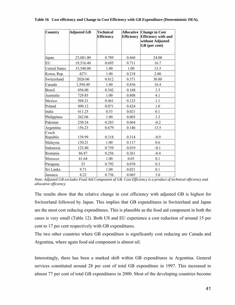
41

Table 16 Cost efficiency and Change in Cost Efficiency with GB Expenditure (Deterministic DEA).

Country Adjusted GB Technical

Efficiency Allocative Efficiency

Change in Cost Efficiency with and without Adjusted GB (per cent)

Japan 23,081.00 0.789 0.468 24.00 EU 19,516.40 0.695 0.711 16.7 United States 15,540.00 1.00 1.00 15.3 Korea, Rep. 4271 1.00 0.218 2.00 Switzerland 2026.06 0.812 0.371 30.80 Canada 1,594.49 1.00 0.836 16.4 Brazil 856.00 0.342 0.168 1.3 Australia 729.85 1.00 0.808 4.1 Mexico 508.21 0.461 0.123 1.1 Poland 490.12 0.071 0.424 1.0 India 411.25 0.53 0.021 0.1 Philippines 262.06 1.00 0.003 1.3 Pakistan 230.24 0.283 0.064 -0.2 Argentina 156.23 0.679 0.146 13.5 Czech Republic 139.99 0.318 0.314 -0.9 Malaysia 130.21 1.00 0.117 0.6 Indonesia 125.40 0.759 0.019 -0.1 Romania 86.87 0.256 0.261 -0.4 Morocco 61.64 1.00 0.03 0.1 Paraguay 25 0.792 0.078 0.3 Sri Lanka 9.71 1.00 0.021 0.1 Jamaica 8.22 0.736 0.065 3.0

Note: Adjusted GB excludes Food Aid Component of GB. Cost Efficiency is a product of technical efficiency and allocative efficiency The results show that the relative change in cost efficiency with adjusted GB is highest for

Switzerland followed by Japan. This implies that GB expenditures in Switzerland and Japan

are the most cost reducing expenditures. This is plausible as the food aid component in both the

cases is very small (Table 12). Both US and EU experience a cost reduction of around 15 per

cent to 17 per cent respectively with GB expenditures.

The two other countries where GB expenditure is significantly cost reducing are Canada and

Argentina, where again food aid component is almost nil.

Interestingly, there has been a marked shift within GB expenditures in Argentina. General

services constituted around 28 per cent of total GB expenditure in 1997. This increased to

almost 77 per cent of total GB expenditures in 2000. Most of the developing countries become

42

relatively less cost efficient with the GB expenditures included in the analysis as the frontier

shifts further inwards.

Stochastic Frontiers

The deterministic DEA analysis which has been used to estimate the impact of GB

expenditures on agricultural productivity and cost efficiency is non parametric and hence is

particularly vulnerable to measurement errors. The deterministic approach constrains the error

term of the cost function to be non-negative. Greene (1980) has shown that the resulting

constant term is consistent but biased and of unreliable efficiency. Nevertheless many studies

have used this approach.

This problem can be overcome using the stochastic cost frontier approach suggested by Aigner

et al. (1977). In this specification the error term is composed of two uncorrelated parts: The

first part ui, is a one-sided non negative disturbance reflecting the effect of inefficiency

(including both allocative and technical inefficiencies), and the second component vit , is a

symmetric disturbance capturing the effect of noise. Usually the statistical noise is assumed to

be normally distributed, while the inefficiency term ui is generally assumed to follow an

exponential or a truncated normal distribution. The main advantage of the stochastic cost

frontier approach compared to the deterministic approach is the separation of the inefficiency

effect from the statistical noise.

To mitigate this concern about deterministic DEA and have robust results of cost efficiency

gains, an attempt has been made to estimate cost efficiency with and without GB using

stochastic frontier cost function. To explain briefly, a stochastic frontier cost function specifies

error term (Vi + Ui) and cost function is defined by:

Yi = xiβ + (Vi + Ui) ,i=1,...,N,

where Yi is the (logarithm of the) cost of production of the ith firm;

xi is a k×1 vector of (transformations of the) input prices and output of the ith

firm;

β is a vector of unknown parameters

the Vi are random variables which are assumed to be iid N(0,σV2), and

independent of the

43

Ui which are non-negative random variables which are assumed to account for

the cost of inefficiency in production, which are often assumed to be iid

|N(0,σU2)|.

In this cost function the Ui now defines how far the firm operates above the cost frontier. If

allocative efficiency is assumed, the Ui is closely related to the cost of technical inefficiency.

If this assumption is not made, the interpretation of the Ui in a cost function is less clear, with

both technical and allocative inefficiencies possibly involved. Thus efficiencies measured

relative to a cost frontier shall be referred to as ‘cost’ efficiencies in the remainder of this

document. The exact interpretation of these cost efficiencies will depend upon the particular

application. The cost frontier is identical to the one proposed in Schmidt and Lovell (1979).

The cost efficiencies have been estimated for countries where the data is available. The data set

is same as that used in determinist DEA cost efficiency gains.

The results in table 17 report the cost efficiency scores which show that with Adjusted GB and

without GB expenditures the relative change in cost efficiency is highest for Canada followed

by EC. This implies that GB expenditures in EC and Canada are the most cost reducing.

Australia, US, Japan and Switzerland also experience a significant cost reduction of around

39.7 per cent, 27 per cent, 25 per cent and 18 per cent respectively with GB expenditures.

The developing countries where Green Box expenditure is significantly cost reducing are

Argentina (15 per cent), where again food aid component is almost nil. Interestingly, there has

been a marked shift within Green Box expenditures in Argentina. General services constituted

around 28 per cent of total Green Box expenditure in 1997. This increased to almost 77 per

cent of total GB expenditures in 2000. As explained above General services and environmental

services had the most significant effect among the GB subsidies.

44

Table 17 Cost efficiency and Change in Cost Efficiency with GB Expenditure

Country

Cost Efficiency

Scores With GB

Cost Efficiency

without GB

Change in Cost Efficiency with GB and without GB ( per cent)

Argentina 17.377 1.6654 15.71 Australia 41.493 1.7912 39.70

Brazil 16.13 1.6471 14.48 Canada 69.568 2.0399 67.52

Czech Republic 9.3704 1.5829 7.78 EC 59.207 4.7419 54.46

India 30.407 4.0334 26.37 Indonesia 13.061 2 11.06

Japan 31.955 6.7133 25.24 Jamaica 3.0902 1.2936 1.79

Korea, Rep. 5.9814 1.9883 3.99 Malaysia 10.284 1.702 8.58 Mexico 8.0995 1.789 6.31

Morocco 52.98 1.5783 51.40 Pakistan 10.781 2.0825 8.69 Paraguay 9.6845 1.3718 8.31

Philippines 4.2649 1.8335 2.43 Poland 7.8626 1.6532 6.20

Romania 19.153 1.3491 17.80 Sri Lanka 61.186 1.6162 59.56

Switzerland 20.458 1.7667 18.69 United States 29.738 2.8335 26.90

Minor gains for other developing countries are observed and this is in line with expectations,

given the small magnitude of GB provided by developing countries

Comparing these results with deterministic DEA cost efficiency as reported in Table 16,

efficiency gains can be noted for all countries due to GB, though the value of efficiency gains

is different from each method. These differences are inevitable because the two approaches are

based on different assumptions. The stochastic DEA assumes a functional form while

deterministic DEA assumes a mathematical relation. The former has an error term while the

latter does not. Both methods have their advantages and disadvantages, so neither is clearly

preferable (Resti 2000; Reinhard, Lovell, and Thijssen 2000;). Despite the differences, both the

DEA approaches (stochastic and deterministic) provide that GB has significant cost reducing

effect for developed countries. However there are some limiting assumptions in stochastic

DEA which do not accord with our understanding of the real world. Therefore, deterministic

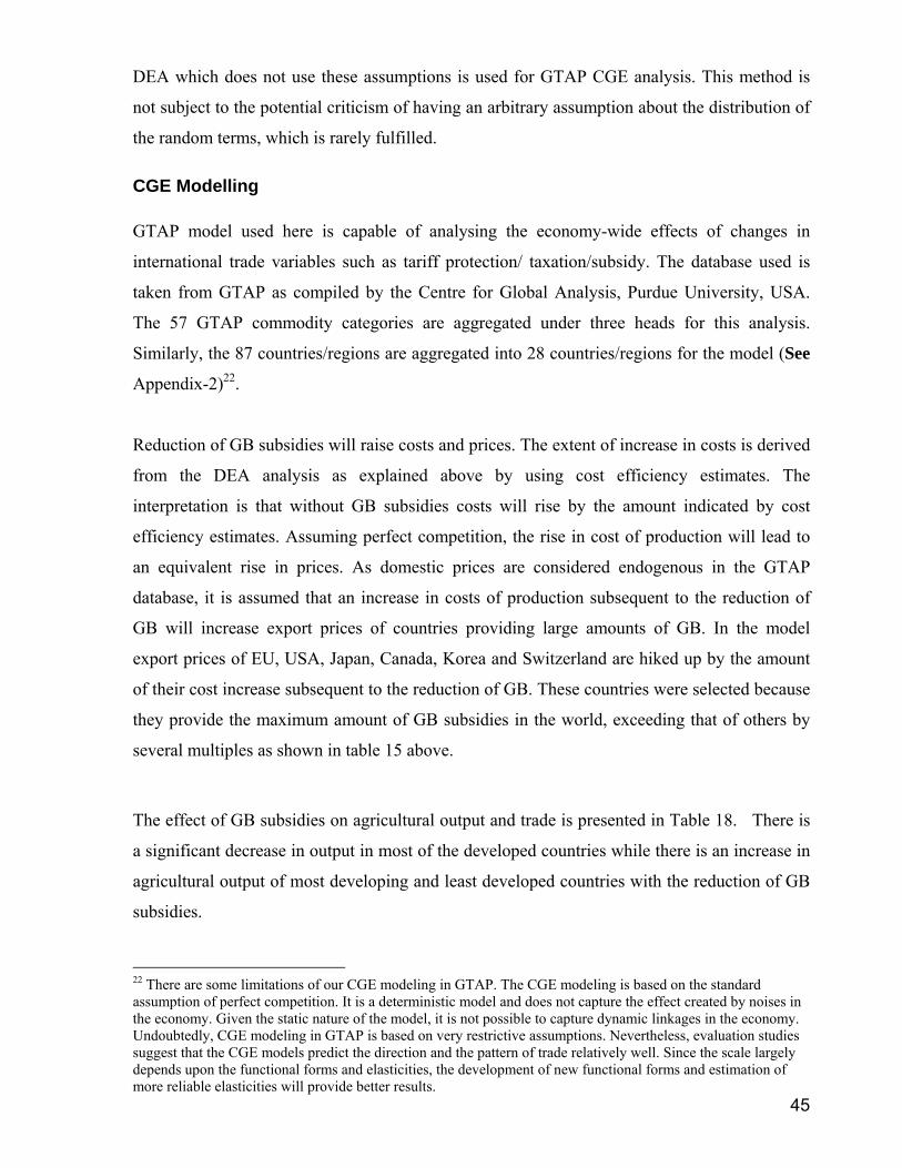
45

DEA which does not use these assumptions is used for GTAP CGE analysis. This method is

not subject to the potential criticism of having an arbitrary assumption about the distribution of

the random terms, which is rarely fulfilled.

CGE Modelling GTAP model used here is capable of analysing the economy-wide effects of changes in

international trade variables such as tariff protection/ taxation/subsidy. The database used is

taken from GTAP as compiled by the Centre for Global Analysis, Purdue University, USA.

The 57 GTAP commodity categories are aggregated under three heads for this analysis.

Similarly, the 87 countries/regions are aggregated into 28 countries/regions for the model (See

Appendix-2)22.

Reduction of GB subsidies will raise costs and prices. The extent of increase in costs is derived

from the DEA analysis as explained above by using cost efficiency estimates. The

interpretation is that without GB subsidies costs will rise by the amount indicated by cost

efficiency estimates. Assuming perfect competition, the rise in cost of production will lead to

an equivalent rise in prices. As domestic prices are considered endogenous in the GTAP

database, it is assumed that an increase in costs of production subsequent to the reduction of

GB will increase export prices of countries providing large amounts of GB. In the model

export prices of EU, USA, Japan, Canada, Korea and Switzerland are hiked up by the amount

of their cost increase subsequent to the reduction of GB. These countries were selected because

they provide the maximum amount of GB subsidies in the world, exceeding that of others by

several multiples as shown in table 15 above.

The effect of GB subsidies on agricultural output and trade is presented in Table 18. There is

a significant decrease in output in most of the developed countries while there is an increase in

agricultural output of most developing and least developed countries with the reduction of GB

subsidies.

22 There are some limitations of our CGE modeling in GTAP. The CGE modeling is based on the standard assumption of perfect competition. It is a deterministic model and does not capture the effect created by noises in the economy. Given the static nature of the model, it is not possible to capture dynamic linkages in the economy. Undoubtedly, CGE modeling in GTAP is based on very restrictive assumptions. Nevertheless, evaluation studies suggest that the CGE models predict the direction and the pattern of trade relatively well. Since the scale largely depends upon the functional forms and elasticities, the development of new functional forms and estimation of more reliable elasticities will provide better results.

46

Table 18 Estimated Effect of GB subsidies on Production and Trade (percentage change)

Countries Output Imports Exports Other Developed Countries (Devd) 10.31 -5.94 15.62 European Union -5.62 -21.27 -44.56 United States of America -2.23 -16.06 -39.03 Canada -9.19 -24.05 -46.33 Argentina 4.32 -2.66 13.76 Australia 7.28 -10.55 16.75 Norway 10.59 -14.54 26.36 Brazil 5.13 -4 21.04 Chile 5.9 -2.24 17.98 India 1.22 -5.77 21.87 Venezuela 1.69 -11.22 26.85 Indonesia 3.11 -7.56 15.89 Thailand 5.01 -3.38 10.06 Morocco 5.53 -13.25 23.75 Poland 3.98 -15.92 25.53 South Africa 6.45 -5.98 24.73 Switzerland -7.74 -20.13 -77.98 Romania 2.11 -12.7 28.8 Slovenia 7.04 -13.04 21.22 Peru 3.3 -7.12 19.57 Japan 1.24 -12.39 -66.49 Korea 2.59 -6.84 3.85 Philippines 2.14 -8.24 14.04 Mexico 3.13 -20.36 14.87 Czech Republic 6.16 -13.34 25.4 Malaysia 9.13 -0.41 13.48 Developing Countries (DCs) 3.51 -11.14 22.04 Least Developed Countries (LDCs) 3.05 -8.52 20.54

For instance, agriculture output in US, EU, Canada and Switzerland decreases by -2.23, -5.62,

-9.19 and -7.74 percent. A plausible reason for why output does not decline very substantially

in US after the removal of GB subsidies as compared to other countries like EU and Canada

can be that the US is found to be closer to the frontier without GB subsidies (Table 19). As a

result removal of GB does not affect its output much. However, exports of US fall more than

proportionately without GB subsidies since in this scenario other countries become relatively

more competitive in agriculture than US. The decline in output is maximum in Canada and

Switzerland pointing perhaps to the fact that technical efficiency in these countries in a static

sense may not be high, hence reduction of GB would lead to a substantial increase of about 16

per cent in the cost of production. At the same time the increase in output is the highest in

competitive agricultural countries such as Argentina, Chile, Brazil, and South Africa which

47

register production increases between 4.5 and 7 per cent. Overall global agricultural output

rises by 0.13 percent (Table 19). While this increase is marginal, the non-negative effects on

global output, contradict predictions about global food shortages consequent to the reduction of

GB. These results also highlight the redistribution of global output in favour of competitive

agricultural producers especially developing countries, and a commensurate reduction in trade

distorting production of developed countries.

Table 19 Country Specific and Global Change in Agricultural Output. (US$ Million)

Countries Percent Change With GB Without GB Absolute change

Other Developed Countries (Devd) 10.31 17094.37 18856.04 1761.67 European Union -5.62 958104.38 904272.75 -53831.63 United States of America -2.23 937664.69 916747.75 -20916.94 Canada -9.19 88035.23 79943.86 -8091.38 Argentina 4.32 58978.22 61523.78 2545.55 Australia 7.28 55137.92 59154.29 4016.37 Norway 10.59 17084.35 18892.78 1808.43 Brazil 5.13 103984.17 109322.76 5338.59 Chile 5.9 23097.45 24459.48 1362.03 India 1.22 172003.7 174098.09 2094.39 Venezuela 1.69 32032.13 32574.2 542.07 Indonesia 3.11 58997.15 60829.75 1832.6 Thailand 5.01 36652.18 38490.05 1837.88 Morocco 5.53 13933.85 14704.79 770.94 Poland 3.98 54688.13 56865.82 2177.7 South Africa 6.45 25382.66 27020.75 1638.08 Switzerland -7.74 22277.19 20552.73 -1724.46 Romania 2.11 19120.72 19524.04 403.32 Slovenia 7.04 4227.29 4525.04 297.76 Peru 3.3 17663.55 18246.02 582.46 Japan 1.24 392428.09 397310.19 4882.09 Korea 2.59 70005.57 71819.27 1813.7 Philippines 2.14 38239.2 39058.18 818.98 Mexico 3.13 140705.92 145111.56 4405.64 Czech Republic 6.16 15760.31 16731.51 971.21 Malaysia 9.13 15657.58 17087.27 1429.69 Developing Countries (DCs) 3.51 1194329.25 1236293.13 41963.88 Least Developed Countries (LDCs) 3.05 180261.19 185761.94 5500.75 Total Output 0.13 4763546.44 4769777.82 6231.38

48

Because of the rise in prices following the reduction of GB, imports of all countries would

decrease as shown in table 18, with Switzerland, EU and Canada showing the highest decline

of over 20 per cent. This could lead to increased self-sufficiency in agriculture at the global

level. Exports from developing countries increase include those from LDCs, while those from

developed countries decrease significantly. For example, agricultural exports from US, EU,

Canada and Switzerland decrease by 40–80 per cent, while exports from developing countries

increase by as much as 26 per cent. Exports from LDCs also register a non-negligible increase.

The changing pattern of international trade in agriculture would also help meet the

development objectives of the Doha Work Programme.

The effects on employment of reducing GB subsidies are presented in Table 20. Agricultural

employment of unskilled labour in developing countries rises while those in developed

countries fall. For instance, agricultural employment in US, EU, Canada and Switzerland

decreases between 2 and 10 per cent, while that of the most competitive developing countries

increases by as much as 7 per cent. Only with few exceptions, the extent and direction of

employment effect follow output effects. In the group of major GB subsidy providers, EU and

Canada see a sharper fall in agricultural employment in comparison to the US. Similarly, more

competitive countries gain more in terms of employment compared to less competitive ones.

Further, there is a 1.13 percent increase in global agricultural employment, implying positive

livelihood effects on agricultural labour. The distributional changes in employment would also

favour developing countries.

Table 20 Employment Effect of removal of GB in Agricultural Sector (Percentage Change)

Countries Unskilled Labour

Skilled Labour

Other Developed Countries (Devd) 10.83 11.25European Union -5.83 -5.9United States of America -2.41 -2.43Canada -9.88 -9.99Argentina 5.09 5.21Australia 8.15 8.37Norway 11.05 11.13Brazil 5.72 5.67Chile 6.81 7.34India 1.66 1.88Venezuela 1.91 2.04Indonesia 4.09 4.78Thailand 7.3 8.14Morocco 5.9 6.66

49

Poland 4.48 4.71South Africa 7.08 7.13Switzerland -8.04 -8.09Romania 2.49 2.82Slovenia 7.61 7.69Peru 3.59 3.95Japan 1.32 1.33Korea 4.03 4.16Philippines 2.52 3.41Mexico 3.43 3.59Czech Republic 6.87 7.03Malaysia 11.31 11.71Developing Countries (DCs) 4.22 4.62Least Developed Countries (LDCs) 3.51 4.11Global Changes 1.13 -1.11

Commensurate with increased agricultural employment, wages of unskilled labour in

developing and poor countries rise, while they fall for some developed countries (Table 21). It

can be inferred from these results that the reduction of GB subsidies would have poverty

alleviating effects, not only through increasing agricultural employment but also through

improving wages.

Table 21 Impact on Agricultural Wages. (Percentage Change).

Countries Unskilled Labour Wages Other Developed Countries (Devd) 2.780529 European Union -0.450762 United States of America -0.151978 Canada -0.665886 Argentina 2.378934 Australia 1.525185 Norway 0.418581 Brazil 1.462496 Chile 1.645657 India 0.704635 Venezuela 0.122378 Indonesia 1.083255 Thailand 1.315871 Morocco 1.726833 Poland 0.659784 South Africa 0.693952 Switzerland -0.315677 Romania 0.372775 Slovenia 0.238892 Peru 1.45782 Japan 0.059904 Korea -0.053932 Philippines 2.130142

50

Mexico 0.405212 Czech Republic 0.458339 Malaysia 0.284838 Developing Countries (DCs) 0.578129 Least Developed Countries (LDCs) 1.61251 Global Changes

The effect of elimination of GB subsidies on Net Food Importing Countries (NFICs) as a group

is also computed. Tables 22–24 show the results. Removal of GB increases the agricultural

production of NFICs by 4.14 per cent. Their imports decline by 10.32 per cent and exports

increase by 22.59 per cent. Further it can be seen that in absolute terms the value of their

increase in production is about three times the value of decline in their agricultural imports.

Hence it is quite clear that the welfare of NFICs also increase as a result of elimination of GB

expenditure.

Further, the positive effect of employment increase in the agriculture sector will not be

outweighed by the negative effect of employment decrease in services and industry in absolute

numbers. Table 22 reveals that the sum of the value (wage times quantity) of employment

across all three sectors in all developing and least developed countries is positive.

Table 22 Sum of the Value Change in Employment in All Three Sectors

Country Absolute Values OTHER DEVELOPED COUNTRIES 454.4 EU -10546.4 USA -5560 CANADA -1663.1 ARGENTINA 1980.2 AUSTRALIA 1720.2 NORWAY 221.2 BRAZIL 2305.3 CHILE 280.1 INDIA 1072.4 VENEZUALA 42.3 INDONESIA 374.9 THAILAND 292.9 MOROCCO 224.7 POLAND 378.6 SOUTH AFRICA 284.7 SWITZERLAND -261 ROMANIA 40.4 SLOVENIA 18.1 PERU 158.6

51

JAPAN 825.7 KOREA -72 PHILIPPINES 305.7 MEXICO 494.8 CZECHOSLAVAKIA 79.8 MALAYSIA 92.2 OTHER DEVELOPING COUNTRIES 6838.6 LESS DEVELOPED COUNTRIES 2147.7 Total 2531.2

Table 23 Removal of GB Effect on Net Food Importing Countries (in percentage terms)

Production Qutput USA CAN SWISS JAPAN EU KOREA Developed Developing NFIC Agriculture -2.34 -9.48 -7.8 1.15 -5.75 2.46 6.43 3.08 4.14Manufacturing 0.37 1.84 1.06 -0.05 1.01 -0.04 -1.33 -1.33 -1.58Services 0.03 0.11 0.03 -0.04 0.1 -0.21 -0.3 -0.22 -0.34CGDS 0.09 -0.41 0.05 0.15 -0.26 -0.14 0.37 0.09 0.34 IMPORTS Imports USA CAN SWISS JAPAN EU KOREA Developed Developing NFIC Agriculture -15.67 -23.64 -20.04 -11.85 -21.1 -6.56 -9.99 -9.94 -10.32Manufacturing -0.48 0.1 0.08 -0.22 -0.09 -0.21 0.13 0.16 0.38Services -0.26 -0.77 -0.49 0.24 -0.45 -0.04 0.7 0.56 0.89 EXPORT Exports USA CAN SWISS JAPAN EU KOREA Developed Developing NFIC Agriculture -40.01 -46.97 -78.12 -66.78 -44.9 3.36 20.45 20.2 22.59Manufacturing 1.19 2.84 1.62 -0.43 1.84 -0.16 -2.35 -2.64 -2.6Services 0.24 1.68 0.56 -0.96 0.8 -0.84 -1.84 -1.8 -2.39 Employment Effect Employment in Agriculture USA CAN SWISS JAPAN EU KOREA Developed Developing NFIC Land -0.11 -0.53 -2.28 0.05 -0.45 0.04 0.54 0.27 0.27Unskilled Labour -2.53 -10.19 -8.1 1.22 -5.96 3.83 7.36 3.84 4.52Skilled Labour -2.55 -10.31 -8.15 1.23 -6.04 3.95 7.66 4.16 4.99Capital -2.51 -10.14 -8.12 1.22 -5.93 3.9 7.56 4.08 4.9Natural Resources 0 -0.02 -0.01 0 -0.01 0.01 0.01 0.01 0.01

52

Table 24 Production Effects for NFICs

BASE DATA

Output USA CAN SWISS JAPAN EU KOREA Developed Developing NFIC Agriculture 937664.7 88035.23 22277.19 392428.1 958104.4 70005.57 328956.2 1565215 400859.6 Manufacturing 4427981 418544.7 146655.6 2180048 4468157 423536.4 1077323 4260134 835383.6 Services 12586357 736719.6 263885.8 4759208 9176874 475944.6 1969284 4279807 1324445 CGDS 1990636 144606 47923.26 1059681 1614488 109932.6 368187.1 1084920 321769.3

Absolute Change Agriculture -21979.4 -8350.09 -1737.6 4511.59 -55080.9 1724.99 21167.91 48236.13 16609.06 Manufacturing 16548.5 7706.69 1548.92 -1122.75 45282 -187.25 -14284.1 -56624.5 -13181.9 Services 3247 809.19 69.25 -1898.5 9121 -976.5 -5924.13 -9551 -4490 CGDS 1756.13 -597.75 22.43 1610.5 -4211.25 -155.84 1354.94 1022.38 1109.81 Percentage change Qutput USA CAN SWISS JAPAN EU KOREA Developed Developing NFIC Agriculture -2.34 -9.48 -7.8 1.15 -5.75 2.46 6.43 3.08 4.14 Manufacturing 0.37 1.84 1.06 -0.05 1.01 -0.04 -1.33 -1.33 -1.58 Services 0.03 0.11 0.03 -0.04 0.1 -0.21 -0.3 -0.22 -0.34 CGDS 0.09 -0.41 0.05 0.15 -0.26 -0.14 0.37 0.09 0.34

Table 25 Import Effects for NFICs

Base Data Imports USA CAN SWISS JAPAN EU KOREA Developed Developing NFIC agriculture 55428.15 14682.2 6823.35 58035.79 206909.3 18697.92 49219.25 101877.7 61272.49Manufacturing 1089452 198291.8 80897.83 287201.3 1858508 130385.4 522108.3 1041221 346933.6Services 176125.4 33112.84 14535.52 84888.39 526861.9 27294.37 113653.5 189417.8 82001.82

Absolute Change Imports USA CAN SWISS JAPAN EU KOREA Developed Developing NFIC agriculture -8685.39 -3470.51 -1367.56 -6879.36 -43630.6 -1226.73 -4915.91 -10129.6 -6325.28Manufacturing -5259.5 202.98 61.43 -634.94 -1678.25 -269.92 668.16 1622.88 1324.03Services -461 -254.93 -71.7 205.85 -2350.06 -10.49 795.38 1064.08 727.3 Percentage change Imports USA CAN SWISS JAPAN EU KOREA Developed Developing NFIC agriculture -15.67 -23.64 -20.04 -11.85 -21.09 -6.56 -9.99 -9.94 -10.32Manufacturing -0.48 0.1 0.08 -0.22 -0.09 -0.21 0.13 0.16 0.38Services -0.26 -0.77 -0.49 0.24 -0.45 -0.04 0.7 0.56 0.89

53

Conclusion In this section, DEA and CGE modelling were applied to see the trade and production

distorting effects of GB. From the DEA analysis it was found that GB expenditures had an

impact on productivity and cost efficiency of agricultural production. Plugging in the results of

the DEA in the CGE model it was found that GB expenditure might also significantly affect

agricultural output, imports, exports, wages and employment. Given the assumptions of CGE

model, the analysis is focused on the direction of the effects. Despite the assumptions and

proxies the CGE result appears quite consistent with the theoretical framework described

earlier. Briefly, seven broad inferences may be drawn. First, agricultural production will

increase in developing countries if GB subsidies are reduced; second, there will be mild

positive impact on global agricultural production; third, agricultural imports will decline,

leading countries towards greater self sufficiency; fourth, there are significant gains for

developing countries in terms of export increase; fifth, agricultural wages in developing

countries will rise; sixth, there will be an increase in agricultural employment in developing

countries as well as global agricultural employment, implying positive livelihood effects on

agricultural labour, and poverty alleviating effect on rural people in developing and poor

countries and seventh, agricultural production will increase in net food importing countries.

Therefore, it can safely be concluded that GB subsides offered by developed countries are

production enhancing and trade distortive.

54

IV. TRANSLOG AND COBB DOUGLAS COST ESTIMATES The DEA analysis in the previous section depicted that GB subsidies have a productivity

enhancing and cost reducing impact on agricultural production of countries that provide them.

To ensure that the results are robust a detailed analysis of GB subsidies and its various

components on the cost of production of five major crops in the US has been conducted. A

Translog cost function has been estimated using panel data for the period 1975–200423. Crop

wise analysis, using a Cobb Douglas function for five different crops- rice, wheat, soybean,

corn and cotton— which constitute the majority of crop production in the US has also been

conducted.

Translog Cost Function A translog function24 is used to estimate the direct and indirect effects of explanatory variables

such as input prices and subsidies on cost of production. A translog function is a combination

of all possible first and second order terms in the logarithms of independent variables such as

output, input prices and GB subsidies. The popular approach to estimating translog cost

function is the share equation approach using Shepherd’s lemma25, which states that a small

increase in the price of an input increases cost by an amount equal to the use of that input. The

translog function contains a large number of parameters even for a relatively small number of

inputs and outputs. As a result, its estimation via ordinary least squares is likely to result in

imprecise parameter estimates due to multicollinearity26. In order to obtain robust estimates of

23 The data for Green Box is available for the base years 1985–6 and then from 1995–6 onwards. It is assumed that no Green Box expenditures were given prior to 1985–6. From 1985–6 to 1995–6, same values of Green Box expenditures are assumed. 24 The translog specification carries large number of cross products terms as explanatory variables in the right side of the equation which sometimes causes multicollinearity. In small sample size, the estimation of translog cost function becomes less reliable as the degrees of freedom are small. Further, the coefficient of translog cost function has complex interpretation. At the same time, the advantage of using the translog specification is that separability between inputs and outputs is not imposed a priori as in the case with the Cobb-Douglas and the CES specifications. 25 Using Shepherd’s lemma, the following share function for each input may be obtained.

, where Si is the cost share of input i. See Appendix 4. 26 Multicollinearity stands for correlation between two explanatory variables. The presence of high correlation distorts the results.

55

standard errors, bootstrapping27 has been used. Generalized Least Squares method which

corrects for heteroscedasticity28 and autocorrelation29 is also applied.

Variables and Data Sources Translog cost functions are estimated for adjusted GB subsidies and also for the individual

constituents—subsidies on general services, subsidies for environmental programmes and

decoupled payments. It is not possible to take all three constituents simultaneously because

subsidies on general services and environmental services are highly correlated with a

correlation coefficient of 0.99. The results for each translog specification are given in Tables

25–28.

The data on cost is constructed from available inputs and their prices. The data on agricultural

output (y), cost of production (cost), rent (ldpcp), wages (lbpcp), interest rate (int), fertilizer

price (Fertcp) are obtained from the website of US department of agriculture30. Expenditure on

GB subsidies31 (gbdef), subsidies on general services (gsdef), environmental subsidies (env)

and decoupled payments (decoup) are obtained from WTO notifications. Squared term for

output (ysq), and GB subsidies and its constituents (gbdefs, gsdefs, envdefs, decoups) are

constructed from original series. Similarly, cross price terms are generated by multiplying the

price variables (intfertcp, rentfertcp, rentwages, wageint, wagefertcp). The cross products of

subsidies and output are also generated from the log of original data (ygb, ygs, yenv, ydc)32.

The interaction term of output with interest, wage rate, rent and fertilizer price (yint, ywagecp,

yrentcp, yfertcp) are obtained by multiplying the log values of output with log values of input

prices. The interaction term of GB subsidies and its constituents with interest, wage rate, rent

and fertilizer price (Gfertcp, Grentcp, Gwagecp, Gint,Gsfertcp, Gsrentcp, Gswagecp, Gsint

Envfertcp, Envrentcp, Envwagecp, Envint, Envwagecp, Envint, Dcfertcp, Dcrentcp,

27 Bootstrapping is the statistical procedure which uses the process of repeated sampling from the population to reduce sampling errors. 28 Violation of the assumption of constant variance over whole range of data, that is, statistically

assumption is 222 )()]([ σ==− iii uEuEuE 29 Violation of the assumption of no covariance in residuals over time, i.e, statistically assumption is 0)()]}()][({[),cov( ==−−= jijjiiji uuEuEuuEuEuu 30 http://www.usda.gov/wps/portal/usdahome 31 Expenditures on public stock holding, domestic food aid, relief from natural disasters has been removed. 32 Ygb, ygs,yenv and ydc are the cross products of output with total green box subsidies, general services, environmental services and decoupled payments respectively.

56

Dcwagecp, Dcint ) are obtained by multiplying the log values of subsidies to log values of

input prices.

Translog Cost Specification with regard to Total GB Subsidies The parameter estimates for the translog cost specification with total GB are given in Table 26.

The coefficient of interest rate, quadratic term of GB, interaction effect of output with fertilizer

price, interest rate, and interaction effect of GB with wages, fertilizer price and few cross price

terms are found to be significant at 5 per cent . The results indicate that cost decreases as

interest increases, which may be attributed to the fact that farmers use GB subsidies for

investing, consequently demand for borrowed money decreases. Considering only the direct

effect of GB, the results depict that every 1 per cent increase in GB reduces the elasticity of

cost with respect to GB by 0.16 units. The interaction effect of GB with fertilizer price

indicates that with every 1 per cent increase in GB subsidies the share of fertilizer in total cost

increases by 0.484 units. The interaction effect of GB with wages (Gwagecp) shows that share

of labour cost decreases by 0.278 units due to 1 per cent increase in GB subsidies. Thus due to

GB, wage share decreases in total cost while fertilizer share increases. If there is any increase

in fertilizer price, wage share in total cost further reduces as the interaction term of labour and

fertilizer price is negative and significant.

The reduction of cost may be attributed to the fact that different kinds of subsidies given under

the variety of programmes might be reinforcing each other to reduce the cost of production.

Second, GB subsidies reduce the cost of production by influencing negatively factor share cost

of labour in total cost. However, it increases the factor share of fertilizer cost in total cost. It

might be inferred from these results that GB subsidies have labour reducing effects. The results

also indicate movement towards capital intensive agriculture due to GB subsidies.

The labour reducing effect of GB seems logical when the nature of US technical change and

research and extension services are considered. Technical change in US agriculture has been

labour-saving since agricultural labour is a relatively scarce. Hayami and Ruttan’s (1985)

induced innovation hypothesis predicts that technologies will be developed that conserve on

relatively scarce factors of production. GB subsidies seem to be an important instrument in the

development of labour saving technology in the US.

57

Table 26 Translog Cost Function With GB Subsidies.

lncost Coef. z

lny 25.61 0.20

Lnldpcp -103.40 -1.22

Lnlbpcp 50.80 1.07

Lnint -36.62 -2.17*

Lnfertp 0.39 0.27

lngbdef -3.69 -0.77

gddef -0.16 -8.32*

ysq -1.60 -0.23

Ywagecp -2.31 -1.01

Yrentcp 4.67 1.16

Yfertcp 0.59 3.06*

Yint 1.95 1.98*

Ygb .07 0.35

Grentcp -.09 -1.08

Gwagecp -.27 -2.95*

Gint -.07 -1.10

Gfertcp .48 2.27*

Rentint -5.27 -3.69*

rentfertcp -1.33 -1.05

Rentwages 10.68 2.02*

Wageint 3.4 2.72*

Wagefertcp -14.42 -5.21*

Intfertcp 0.91 0.98

_conss -2159 1.92*

years

* indicates statistically significant at 5% level of significance

Existing literature explains various ways in which GB subsidies reduce cost. For instance, there

are intuitive reasons to expect agricultural research and extension as well as inspection services

(sanitary, phytosanitary, grading, certification and consumer protection) to reduce production

and transaction costs. Similarly, Structural adjustment payments might help induce high-cost

parcels of land and high-cost producers to exit the agricultural sector, reducing industry-wide

average cost.

On the basis of above discussion, it is easy to infer that removal of subsidies may be beneficial

to agriculture labour in the US. There is convincing statistical evidence which confirms the

58

concentration of existing farm programme payments among large producers and agribusiness.

This is well-recognized in reports by ERS. e.g., a report in the February 2005 issue of the ERS

publication Amber Waves on growing farm size and the distribution of commodity program

payments.

(http://www.ers.usda.gov/AmberWaves/February05/DataFeature/).

Translog Cost Specification with regard to General Services The parameter estimates for the translog cost specification with subsidies on general services

are given in Table 27. It can be seen that subsidies on general services reduce costs of all

factors of production. This cost reduction may be attributed to the various programmes under

general services which have production enhancing and cost reducing effects. For instance,

agriculture research service reduces cost of production by developing new techniques and

methods for protection and storage of agricultural production. Subsidies under public research

and extension expenditures might also enhance agricultural productivity. Higher productivity

raises output and causes prices to fall, but does not impoverish farmers because the

productivity gains also lower their costs of production. (David, Kaukab, and Bonilla 2002).

Table 27 Translog Cost Function With Subsidies On General Services.

lncost Coef. z

lny -27.16 -0.50

Lnldpcp -93.16 -2.00*

Lnlbpcp 35.81 0.95

Lnint -35.77 -3.01*

Lnfertp -1.46 -1.12

lngsdef -3.46 -1.58

gsdefs -0.11 -2.61*

ysq 0.90 0.30

Ywagecp -1.63 -0.91

Yrentcp 4.14 1.91

Yfertcp 0.65 4.27*

Yint 1.90 2.21*

Ygs 0.05 0.52

Gsrentcp -0.12 -2.42*

lncost Coef. z

Gswagecp -0.30 -5.74*

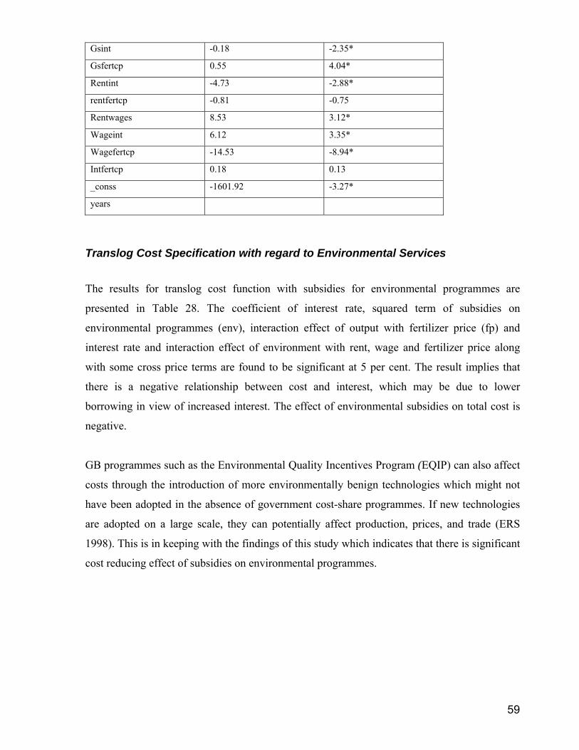
59

Gsint -0.18 -2.35*

Gsfertcp 0.55 4.04*

Rentint -4.73 -2.88*

rentfertcp -0.81 -0.75


Wageint 6.12 3.35*


Intfertcp 0.18 0.13

_conss -1601.92 -3.27*

years

Translog Cost Specification with regard to Environmental Services

The results for translog cost function with subsidies for environmental programmes are

presented in Table 28. The coefficient of interest rate, squared term of subsidies on

environmental programmes (env), interaction effect of output with fertilizer price (fp) and

interest rate and interaction effect of environment with rent, wage and fertilizer price along

with some cross price terms are found to be significant at 5 per cent. The result implies that

there is a negative relationship between cost and interest, which may be due to lower

borrowing in view of increased interest. The effect of environmental subsidies on total cost is

negative.

GB programmes such as the Environmental Quality Incentives Program (EQIP) can also affect

costs through the introduction of more environmentally benign technologies which might not

have been adopted in the absence of government cost-share programmes. If new technologies

are adopted on a large scale, they can potentially affect production, prices, and trade (ERS

1998). This is in keeping with the findings of this study which indicates that there is significant

cost reducing effect of subsidies on environmental programmes.

60

Table 28 Translog Cost Function With Environmental Subsidies.

lncost Coef. z

lny -1.37 -0.01

Lnldpcp -75.89 -1.04

Lnlbpcp 3.98 0.09

Lnint -31.36 -2.64*

Lnfertp -0.81 -0.50

Env 0.85 0.30

Envdefs -0.16 -3.41*

ysq -0.004 -0.0

Ywagecp -0.17 -0.08

Yrentcp 3.30 0.95

Yfertcp 0.34 3.67*

Yint 1.68 2.80

Ygb -0.12 -0.99

Envrentcp -0.20 -2.21*

Envwagecp -0.34 -5.32*

Envint -0.16 -1.22

Envfertcp 0.44 2.22*

Rentint -4.93 -3.72*

rentfertcp 1.015 1.21

Rentwages 3.35 1.37

Wageint 4.63 1.69


Intfertcp 0.46 0.34

_conss -1927.91 -1.86

61

Translog Cost Specification with regard to Decoupled Payments Table 29 Translog Cost Function With Decoupled Payments.

lncost Coef. z

lny 109.43 2.81*

Lnldpcp -9.04 -0.11

Lnlbpcp 40.58 1.70

Lnint -37.11 -0.50

Lnfertp -1.65 -0.71

Lndecoudef -8.21 1.20

decoups -0.046 -8.54*

ysq -5.39 -3.51

Ywagecp -2.00 -1.79

Yrentcp 0.29 0.08

Yfertcp 0.86 3.78*

Yint 1.41 0.45

ydc 0.23 -0.03

Dcrentcp -0.0028 -3.66*

Dcwagecp -0.28 -2.59*

Dcint -0.30 7.14*

Dcfertcp 0.79 0.22

Rentint 0.42 -15.17*

Rentfertcp -3.37 3.13*


Wageint 7.67 -8.58*

Wagefertcp -15.39 0.90

Intfertcp 1.76 0.83

_conss -3105.61 -6.24

Years

The result for translog cost function with subsidies for decoupled payments (DP) are given in

Table 29. The coefficient of output, quadratic term of decoupled payments, quadratic term of

output, interaction effect of output with wage, fertilizer price and interest rate and interaction

effect of decoupled payments with rent, wage and fertilizer price along with some cross price

terms are found to be significant at 5 per cent level of significance. There is a negative effect

on costs due to decoupled payments. Increase in decoupled payments has a negative effect on

62

interest rate due to increased cash flow to the farmers and resultant decrease in demand for

borrowed resources. The decreasing interest rate further leads to labour reduction. Increased

cost share of fertilizers in total cost is also apparent with decoupled payments due to indirect

effects arising from reduced risk, enhanced cash flow, or increased producer wealth.

Furthermore, government payments to field crop farmers in the US in the form of PFCs and

MLAs stimulate higher production because some fixed costs are covered. This induces farmers

to stay on the land because of reduction in risks of production and increased expectations for

more support in the future (de Gorter 2001). Market signals are masked, with the result that

producer decisions are made in response to the decoupled payments rather than to the market

(Grey, Clark, Shih and Associates, Limited, 2006). The result of present study also indicates

cost reducing effect of DC.

The translog cost function explicitly depicts the cost decreasing effect of subsidies provided

under GB. The result indicates that subsidies have a fertilizer augmenting effect and labour

reducing effect. The inference from the above discussion is that GB subsidies are cost reducing

and therefore refute the premise that GB subsidies are not trade distorting and production

enhancing.

Crop-Wise Results

GB subsidies might have differential production effects on different crops. In order to analyse

this, a Cobb Douglas Cost function is used to estimate the impact of GB subsidies on the cost

of production of five major crops. The crops used in our analysis are soybean, corn, cotton, rice

and wheat. These products constitute around 81 per cent of total crop production in US. The

three most important crops in the US are currently corn, soybeans and wheat. These three crops

account for about 87 per cent of acreage for the eight major US field crops and over 60 per cent

of acreage for all US field crops. Rice acreage has risen from 650 thousand ha in 1960 to about

1.4 million ha in 2005, however, it remains small compared to corn, soybeans or wheat. Since

it is not possible to estimate the share of GB expenditures with respect to each crop, it is

assumed that each crop benefits equally from all categories of GB expenditures. For example if

infrastructure subsidies are granted production of all crops will benefit equally. Therefore the

effect of total GB expenditures on cost of production of each crop is estimated.

63

Variables and Data Sources

The model estimated is:

C(q; gb ; wL,wK,wM) = h(q) * c(wL,wK,wM)

Where C is cost; q is output; gb is GB expenditures/general services expenditures/ environment

services/ decoupled payments; wL is wages paid to agricultural labour; wK is cost of capital

and wM is cost of inputs like fertilizers.

Constant returns to scale are assumed. Using data from 1975 to 2004, the cost function is

estimated using a time-series analysis. Cochrane Orcutt AR (1) regressions are estimated.

Separate equations are estimated using log of deflated GB expenditures (lngbdef), log of

deflated general services (lngsdef), log of deflated environment services (lnenvr) and log of

deflated decoupled payments (lndecoud)33.

The variables used are as follows:

1. Land: Data from USDA on land under cultivation in different crops deflated by land

price series.

2. Labour Prices: Real wage rates collected from World Development Indicators, 2006.

3. Capital price: Number of tractors (also used by Coelli and Prasada Rao 2003) and their

imported price has been used for capital price. Annualized flows of capital are used.

4. Fertilizer prices: Data collected from USDA at Constant price s.

5. GB Expenditures: Data from WTO notifications. To arrive at constant price series,

GDP implicit deflators have been used.

Empirical Results

Studies show that under the existing US policy, the cost of producing major crops has been

much higher than the prices realized for them. In the year 2001, market prices were 23 per cent

below the cost of production for corn, 48 per cent for wheat, 32 per cent for soybean, 52 per

cent for cotton, and 45 per cent for rice(Ray et al, 2003).In 2001 US had a significant share in

world exports in these commodities which is as high as 35 per cent in cotton, more than 20 per

cent in wheat and around 10 per cent in rice.

33 High correlation coefficient was found between lngsdef and lnenvr. To check omitted variable bias an equation including all three components of GB expenditures was run and significant coefficient were found for lngsdef and lndecoud

64

According to the Farm Bill 2002 commodity programme, ‘farmers who participated in the

wheat, corn, barley, grain sorghum, oats, upland cotton, and rice programs in any one of the

years 1991–5 could enter into 7-year production flexibility contract for 1996–2002 during a

one-time enrollment period.’ This implies that the subsidies given earlier continue. Direct

payments are available for eligible producers of wheat, corn, barley, grain, sorghums, oats,

upland cotton and rice. Allocation of these payment levels are: 26.26 per cent for wheat, 46.22

per cent for corn, 11.63 per cent for upland cotton and 8.47 per cent for rice. Payment rates

specified are $0.52 per bu for wheat, $ 0.28 per bu for corn, $0.44 per bu for soybean and

$2.35 per cwt for rice. Loan rates also differ across crops and are provided on a per-unit value

to farmers via commodity secured loans. Loan rates for 2002–03 were fixed at $2.80 per bu for

wheat, $1.98 per bu for corn, $6.50 per cwt for rice and $5.00 per bu for soybean and $0.52 per

lb for upland cotton

This makes it important to carry out crop-wise estimates of effects of GB expenditures and its

components on crop-wise cost of production. However, since the number of available

observations is only 30, these estimates may not have the desired robustness.

A cursory look at the data gives some important insights. Over time, it is found that rate of

interest on operating capital in terms of dollars per acre for different crops decline in the period

1996 to 1999 and between 2000 and 2003 (Figure 4).

Figure 4 Interest on Operating Capital .

INTEREST ON OPERATING CAPITAL

0.00

1.00

2.00

3.00

4.00

5.00

6.00

7.00

8.00

9.00

1996

1997

1998

1999

2000

2001

2002

2003

2004

YEARS

INTE

RES

T ($PE

R A

CRE)

Rice

Wheat

Corn

SoybeanCotton

Source- USDA Website

Benefits that accrue to cropland enrolled in US farm are mainly capitalized into land values. It

is found that land prices for rice have increased substantially since the latter half of the

1990s.This might be linked to the fact that the direct payments for rice are relatively high.

Figure 5 Land Prices (US$ per ha).

65

LAND PRICES ($ PER ACRE)

020406080

100120140160180200

1975

1978

1981

1984

1987

1990

1993

1996

1999

2002

Years

Land

pric

es ($

per

acr

e)

Rice

Wheat

Soybean

CORN

Cotton

Source- USDA Website

Wheat The results with respect to wheat presented in Table 30 show that GB expenditures have

reduced the cost of production of wheat by 5.0 per cent. With respect to general services and

environmental services the reduction of cost is around 6 per cent and 7 per cent respectively.

However, the effect of decoupled payments is not found to be statistically significant.

Table 30 Wheat.

Variable Coefficient

(t-values) Coefficient (t-values)

Coefficient (t-values)


Constant -1.85 (-0.80) -1.84 (-0.79) -1.85 (-0.80) -2.28 (-0.88) Lny 0.12 (0.99) 0.12 (1.01) 0.12 (0.99) 0.18 (1.38) lnldp 0.25 (3.94)* 0.25 (3.96)* 0.25 (3.94)* 0.29 (4.92)* lnlbp 0.31 (4.43)* 0.31 (4.37)* 0.31 (4.39) * 0.31 (3.29)* lntracp 0.29 (2.05)* 0.29 (2.04)* 0.29 (2.08)* 0.19 (1.62) lngbdef -0.05 (-2.46)* -- -- -- lngsdef -0.06 (-2.46)* -- -- lnenvr -- -0.07 (-2.57)* -- lndecoud -- -- -0.03 (-0.84) F (6,23) 40137.43 39187.59 39886.54 36071.06 Prob > f 0.00 0.00 0.00 0.00 R-squared 0.88 0.88 0.88 0.88 * depicts that the result is statistically significant

66

Corn The results with respect to corn presented in Table 31 show that GB expenditures reduce the

cost of production of corn by 7 per cent and are found to be statistically significant. The other

three components of GB also have significant impact on cost of production of corn.

Expenditure on general services reduces cost of production by 8 per cent, environment services

by 10 per cent and decoupled payments by 8 per cent. Land prices are not found to add as

significantly to cost of production as in the case of wheat.

Table 31 Corn.

Variable Coefficient (t-values)




Constant 0.51 (0.41) 0.61 (0.62) 0.56 (0.57) 0.61 (0.62) Lny 0.08 (2.73)* 0.08 (0.98) 0.08 (3.02)* 0.08 (2.98)* lnldp 0.16 (1.96)* 0.15 (2.30)* 0.14 (2.24)* 0.15 (2.30)* lnlbp 0.23 (0.78) 0.14 (0.68) 0.14 (0.67) 0.14 (0.68) lntracp 0.25 (3.61)* 0.25 (3.74)* 0.25 (3.81)* 0.25 (3.74)* lngbdef -0.07 (-3.26)* -- -- -- lngsdef -- -0.08 (-3.68)* -- lnenvr --- -- -0.10 (-3.75)* -- lndecoud -- -- -- -0.08 (-3.68)* f (5,23) 17.19 17.95 18.27 10.34 Prob > f 0.00 0.00 0.00 0.00 R-squared 0.78 0.79 0.79 0.69 * depicts that the result is statistically significant

Rice The results with respect to rice presented in Table 32 show that GB expenditures have

considerable impact on cost of production of rice, which goes down by 5 per cent. The impact

of general services and environment services on lowering cost of production are found to be 6

per cent and 8 per cent respectively. However, impact of decoupled payments is not found to

be statistically significant.

Table 32 Rice





constant 1.97 (1.95)* 1.91 (1.90)* 1.85 (1.85) 3.07 (2.86)* lny 0.04 (0.81) 0.40 (0.77) 0.03 (0.74) 0.07 (1.81) lnldp 0.05 (1.56) 0.04 (1.35) 0.04 (1.18) 0.12 (5.90)* lnlbp 0.31 (3.38)* 0.31 (3.52)* 0.31 (3.67)* 0.12 (0.46) lntracp 0.29 (4.21)* 0.30 (4.69) * 0.32 (4.95)* 0.10 (1.64) lngbdef -0.05 (-2.26)* -- -- lngsdef -- -0.06 (-2.40)* lnenvr -- -0.08 (-2.52)* lndecoud -- -- -- f (6,23) 49186.15 52922.20 54427.36 Prob > f 0.00 0.00 0.00 R-squared 0.88 0.90 0.91 * depicts that the result is statistically significant

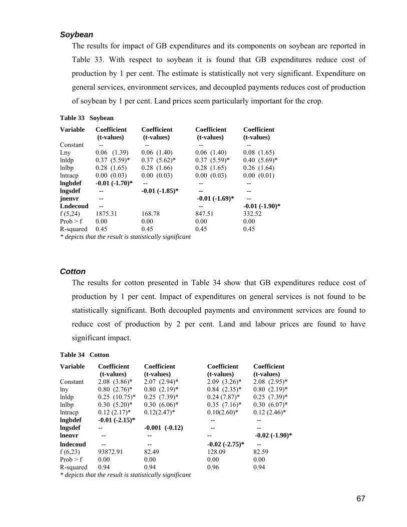
67

Soybean The results for impact of GB expenditures and its components on soybean are reported in

Table 33. With respect to soybean it is found that GB expenditures reduce cost of

production by 1 per cent. The estimate is statistically not very significant. Expenditure on

general services, environment services, and decoupled payments reduces cost of production

of soybean by 1 per cent. Land prices seem particularly important for the crop.

Table 33 Soybean





Constant -- -- -- -- Lny 0.06 (1.39) 0.06 (1.40) 0.06 (1.40) 0.08 (1.65) lnldp 0.37 (5.59)* 0.37 (5.62)* 0.37 (5.59)* 0.40 (5.69)* lnlbp 0.28 (1.65) 0.28 (1.66) 0.28 (1.65) 0.26 (1.64) lntracp 0.00 (0.03) 0.00 (0.03) 0.00 (0.03) 0.00 (0.01) lngbdef -0.01 (-1.70)* -- -- -- lngsdef -- -0.01 (-1.85)* -- -- jnenvr -- -0.01 (-1.69)* -- Lndecoud -- -- -0.01 (-1.90)* f (5,24) 1875.31 168.78 847.51 332.52 Prob > f 0.00 0.00 0.00 0.00 R-squared 0.45 0.45 0.45 0.45 * depicts that the result is statistically significant

Cotton The results for cotton presented in Table 34 show that GB expenditures reduce cost of

production by 1 per cent. Impact of expenditures on general services is not found to be

statistically significant. Both decoupled payments and environment services are found to

reduce cost of production by 2 per cent. Land and labour prices are found to have

significant impact.

Table 34 Cotton Variable Coefficient

(t-values) Coefficient (t-values)



Constant 2.08 (3.86)* 2.07 (2.94)* 2.09 (3.26)* 2.08 (2.95)* lny 0.80 (2.76)* 0.80 (2.19)* 0.84 (2.35)* 0.80 (2.19)* lnldp 0.25 (10.75)* 0.25 (7.39)* 0.24 (7.87)* 0.25 (7.39)* lnlbp 0.30 (5.20)* 0.30 (6.06)* 0.35 (7.16)* 0.30 (6.07)* lntracp 0.12 (2.17)* 0.12(2.47)* 0.10(2.60)* 0.12 (2.46)* lngbdef -0.01 (-2.15)* -- -- lngsdef -- -0.001 (-0.12) -- -- lnenvr -- -- -- -0.02 (-1.90)* lndecoud -- -- -0.02 (-2.75)* -- f (6,23) 93872.91 82.49 128.09 82.59 Prob > f 0.00 0.00 0.00 0.00 R-squared 0.94 0.94 0.96 0.94 * depicts that the result is statistically significant

68

Conclusion: Summarizing the results of the Empirical Analysis This section summarizes the main findings of the empirical analysis carried out in the paper

thus far.

To estimate the impact of GB expenditures on agricultural productivity and cost efficiency

DEA has been used. Initially the total factor productivity growth for 27 countries during the

period 1995–2000 is estimated using Malmquist indices. DEA analysis finds that there has

been an increase in TFP in all the three high GB countries, with Japan experiencing the highest

rise. Countries such as Korea, Switzerland and Thailand also experience a rise in their

productivity with GB expenditures.

Cost efficiencies are also calculated using the input oriented DEA analysis. This analysis finds

that GB expenditure in Switzerland(30%) and Japan(24%) has the highest relative impact on

cost efficiency. This is a plausible result since food aid component in both the cases is very

small. US and EU also experience cost reductions of around 15 per cent to 17 per cent

respectively, while Canada and Argentina also show significant cost reductions. Further it can

also be seen that with GB expenditure most of the developing countries become less cost

efficient since the frontier shifts inwards with increasing efficiency in developed countries.

Since the DEA analysis is non parametric, the paper also uses a parametric approach in which

the Translog cost function is estimated to calculate the direct and interaction effects that GB

subsides and its components may have on the cost of production in the US. The estimation

finds that a 100 per cent increase in GB support leads to 16 per cent reduction in cost of

production. The following results are obtained regarding the impact of certain components of

GB support: (i) 100 per cent increase in general services component leads to 11 per cent

reduction in cost of production; (ii) 100 per cent increase in environmental programme support

under GB leads to 16 per cent reduction in cost of production; (iii) 100 per cent increase in

decoupled income support leads to 4.6 per cent reduction in costs.

In order to estimate the impact of the reduction in cost of production as a result of GB

expenditure on trade and production, the results of the DEA analysis on cost efficiencies are

plugged into the CGE model. Simulating for increase in cost of production on account of

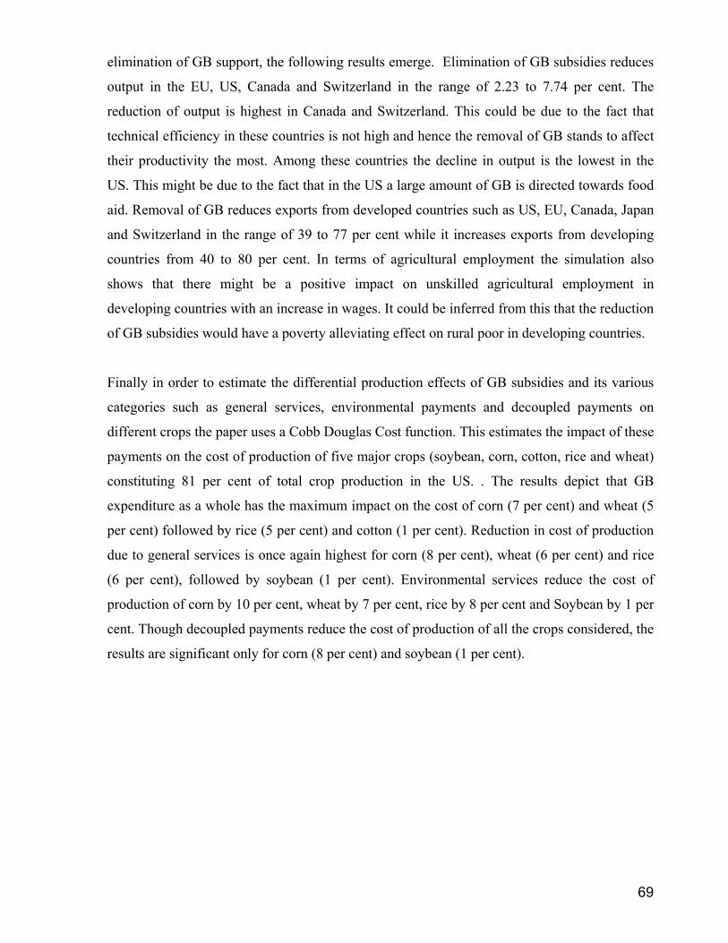
69

elimination of GB support, the following results emerge. Elimination of GB subsidies reduces

output in the EU, US, Canada and Switzerland in the range of 2.23 to 7.74 per cent. The

reduction of output is highest in Canada and Switzerland. This could be due to the fact that

technical efficiency in these countries is not high and hence the removal of GB stands to affect

their productivity the most. Among these countries the decline in output is the lowest in the

US. This might be due to the fact that in the US a large amount of GB is directed towards food

aid. Removal of GB reduces exports from developed countries such as US, EU, Canada, Japan

and Switzerland in the range of 39 to 77 per cent while it increases exports from developing

countries from 40 to 80 per cent. In terms of agricultural employment the simulation also

shows that there might be a positive impact on unskilled agricultural employment in

developing countries with an increase in wages. It could be inferred from this that the reduction

of GB subsidies would have a poverty alleviating effect on rural poor in developing countries.

Finally in order to estimate the differential production effects of GB subsidies and its various

categories such as general services, environmental payments and decoupled payments on

different crops the paper uses a Cobb Douglas Cost function. This estimates the impact of these

payments on the cost of production of five major crops (soybean, corn, cotton, rice and wheat)

constituting 81 per cent of total crop production in the US. . The results depict that GB

expenditure as a whole has the maximum impact on the cost of corn (7 per cent) and wheat (5

per cent) followed by rice (5 per cent) and cotton (1 per cent). Reduction in cost of production

due to general services is once again highest for corn (8 per cent), wheat (6 per cent) and rice

(6 per cent), followed by soybean (1 per cent). Environmental services reduce the cost of

production of corn by 10 per cent, wheat by 7 per cent, rice by 8 per cent and Soybean by 1 per

cent. Though decoupled payments reduce the cost of production of all the crops considered, the

results are significant only for corn (8 per cent) and soybean (1 per cent).

70

V. REVIEW AND CLARIFICATION OF GB CRITERIA: PROGRESS IN NEGOTIATIONS

Under the Agreement on Agriculture, Green Box domestic support is not subject to reduction

commitments. Further, rules and disciplines on GB are not as stringent as those on amber box

support. Unlike amber box support, which was subject to reduction commitments under the

AoA, there is no reduction commitment for GB support. Countries cannot provide amber box

support beyond a prescribed ceiling. However, as there is no upper bound for GB support,

countries can provide any amount under this support subject to meeting the criteria specified in

Annex 2 of AoA.

In the context of the findings of the paper thus far, it is pertinent to look at the current

developments in the GB negotiations as also the proposals put forward by the different

members on reviewing the GB criteria. As per paragraph 16 of the July 2004 Framework, the

WTO members have been mandated to review and clarify the GB criteria to ensure that the

trade or production effects are minimal or absent. This chapter, after setting out the mandate

for review as specified in the July Framework and the Hong Kong Declaration, very briefly

specifies some of the proposals put forth by different members.

Mandate for review and clarification of GB criteria: The July Framework and the Hong Kong Declaration

On the issue of GB support, different members vary in their views. For instance while the G-

20, Canada and Australia argue that some of the criteria for GB spending need to be revised to

minimize distortive impacts, others such as the US and the EU argue against making

substantial changes ( ICTSD, 2006) .. It is in the context of this debate that the July framework

put forth a mandate for review and clarification of the GB criteria (Paragraph 16 of this

Framework (Annex A of WT/L/579)).The modalities of clarifying the GB criteria have been

left to the negotiations. Paragraph 5 of the Hong Kong Ministerial Declaration states that GB

criteria will be reviewed in line with paragraph 16 of the Framework, inter alia, to ensure that

programmes of developing country Members that cause not more than minimal trade-distortion

are effectively covered. What has to be noted here is that while the July framework made no

specific mention of developing countries this declaration specifically does so.

On the basis of discussions held so far, it may be concluded that at a broad level WTO

Members appear to be pursuing two objectives in the process of review and clarification of GB

71

criteria: (i) making the eligibility criteria for developed countries more restrictive; and (ii)

clarifying/ inserting additional criteria for covering programmes of developing countries that

cause no or minimal trade-distortions. While there appears to be considerable openness among

Members to better tailor the GB criteria to meet the realities of developing country agriculture,

there appears to be some resistance to altering the criteria for making it more restrictive.

Paragraph 16 of the July Framework also specifies that the review and clarification will need to

ensure that the basic concepts, principles and effectiveness of the Green Box remain and take

due account of non-trade concerns. Some developed countries are of the view that the current

criteria are adequate, and might even need to be made more flexible to take better account of

non-trade concerns such as environmental protection and animal welfare. These countries are

concerned that any change to the existing green box provisions might have the effect of

undermining their reforms. Thus, there is, on the one side, a firm resistance to anything that is

seen as departing from the existing disciplines while there is, on the other, an enduring sense

that more could be done to review the Green Box34.

Proposals have been made by different WTO members on the different categories of GB

support such as general services, public stock holding for security purposes, domestic food aid,

direct payments to producers, decoupled income support, income insurance and safety net

programmes, natural disaster relief payments, structural adjustment assistance through

retirement programmes and investment aids and regional assistance programmes35. Box 4 very

briefly sets out some of the negotiating proposals.

34 Draft Possible Modalities on Agriculture, JOB(U6)/199 plus corr 1 changes, 22 June 2006 35 Appendix 3 gives a detailed explanation of the proposals in each of these categories.

72

Box 4 Various Negotiating Proposals on GB Subsidies36

Proposals which seek flexibility for developing countries • Extend the coverage of general services to include categories such as agrarian land and institutional reform,

including related services such as settlement programmes and also services related to developing country proposals on food, livelihood security, rural development and infrastructure provision.

• Unambiguous clarification that the acquisition costs of stocks of foodstuffs would be accommodated within the 10 per cent de minimis allowance for developing countries.

• Amend footnotes 5 & 6 (related to paragraphs on stockholding for food security purposes and domestic food aid) to cover the acquisition of foodstuffs at subsidized prices when generally procured from low-income or resource-poor producers in developing countries with the objective of fighting hunger and rural poverty.

• In terms of payments under regional assistance programmes the negotiating proposals seek to exempt developing countries from the requirement that a disadvantaged region must constitute a clearly designated contiguous geographical area with a definable economic and administrative identity

Proposals which seek strengthening of disciplines • Various negotiating suggestions have been put forth regarding direct payments such that they should be

delinked from production levels, including input levels therein; they should be based on activities in a fixed and unchanging historical base period; amend the last sentence of paragraph 5 thereby requiring that direct payments exempt from reduction commitments conform to (a revised) criterion 6(a)37 in addition to criteria 6(b) through (e) of paragraph 6, delete the last sentence of paragraph 5, thereby making paragraphs 6 to 13 the exhaustive list for possible direct payment support.

• In respect of decoupled income support changes have been suggested to constrain some of the eligibility criteria for this support. It has been suggested that eligibility for such support be determined by criteria of low level of income, landholding and production in a notified and unchanging base period. Some countries have suggested adding the criteria that land, labour or any other factor of production should not be required to be in ‘agricultural use’ in order to receive payments. It has also been proposed that an additional sub-paragraph (f) be added to paragraph 6 to reflect that direct payments under paragraph 6 should not be made along with Amber Box or Blue Box support if the total value of support exceeds a certain percentage of the annual value of production of a given product.

• Negotiating proposals have also been made on the eligibility criteria and the payments for income insurance and safety net programmes as also for natural disaster relief programmes.

• In terms of structural adjustment assistance while no proposals have yet been made on resource/producer retirement programmes, for assistance programmes through investment aids it has been proposed that structural disadvantages must be clearly defined in the context of government programmes for reprivatization of agricultural land.

Assessment of GB proposals It may be useful to briefly discuss the specific concerns arising from the implementation of the

Agreement on Agriculture, which the various proposals on GB seek to address. Under

provisions of paragraph 6(a) eligibility for decoupled income support is required to be based on

clearly-defined criteria in a ‘defined and fixed base period’. According to the G-20 proposal,

this has been interpreted by some WTO Members to fix the base period only for specific time

intervals, which are subsequently updated. This reinforces the farmers’ expectations, thereby

influencing their future production decisions. Overall, updating the base year provides farmers

36 Appendix 3 provides further details on the negotiating proposals on GB subsidies. 37 Criteria 6(a) is described in detail on page 96 in paragraph 1.

73

with incentives to keep production levels high. Stipulating base periods which are fixed and

unchanging could remove the incentive for the farmers to maintain high levels of production

so that they become eligible for higher support in case the base period is updated in future. The

proposals seeking to insert ‘a defined, fixed and unchanging historical base period’ in

paragraph 5(a) and ‘unchanging historical base period’ in paragraph 6(a) appear to have been

made in order to address this problem of updating base periods.

Another issue of concern relates to the fact that subsidies in general are concentrated in the

hands of very few entities. Among subsidy recipients in the US, large farms collect almost all

the money. Nationwide, ten per cent of the biggest (and often most profitable) subsidized crop

producers collected 72 per cent of all subsidies amounting to $104 billion over 10 years.

Recipients in the top 10 per cent averaged $33,283 in annual payments between 1995 and

2004. The bottom 80 per cent of the recipients saw only $721 on average per year.38 In order to

address the issue of concentration of decoupled income support in a few entities and to avoid

payments being received by big farmers, G-20 has proposed that eligibility for decoupled

income support should be determined by criteria of low levels of income, landholding and

production39. This proposal could have far-reaching effects. First, it would restrict the

eligibility for receiving decoupled income support to producers, thereby excluding landowners

who are not producers. Second, in order to become eligible for receiving decoupled income

support, the producer must simultaneously satisfy the three criteria of low income, low

production and small landholding.

The proposed change in criteria could ensure that decoupled income support is not available to

agri-business and rich farmers. The benefits of GB would be mainly available to small and

poor farmers. However, what may be a low level of income in a developed country may

represent high income in a developing country. Similarly, a small land holding in a country

with extensive agriculture may not be considered small in a country practicing intensive

farming. For the proposal to be more meaningful, it may therefore be necessary to specify the

indicators for the ‘low level’. To illustrate, income could be categorized as low, if it is 15 per 38 Environmental Working Group’s Farm Subsidy Database accessible at

http://www.ewg.org/farm/region.php?fips=00000 visited on 18 May 2006 ; (G20/DS/Greenbox FINAL 02/06/05) 39 In fact a survey carried out in 2004 by the Program on International Policy Attitudes finds that more than three-quarters of Americans (and 81 per cent of those in farm states) are in favour of the US government giving subsidies to small farmeres who own less than 500 acres, but only 31 per cent (and the same proportion in farm states) are in favour of subsidies for large farming businesses.

74

cent below the per capita income for the country. Similar indicators could be proposed for low

production and low landholding.

Other proposals also seek to address the incentive for increasing production which arises

when coupled support programmes(Amber or Blue Box) are implemented in combination with

GB direct payments on the same product. The World Bank has pointed out that ‘the co-

existence of coupled and decoupled programmes means that incentives to overproduce

remain’40. In the EU, member states have the option to keep part of the payment linked to crop

and livestock production. Up to 25 per cent of the payments for arable crops, and 50 to 100 per

cent of animal payments may remain linked, or coupled. France and Spain have both made use

of this option in the case of area payments. Cereal farmers who stop production, or shift to

livestock production, for example, receive only 75 per cent of their previous payments, and

have to cover the costs of keeping the land in good condition. If they continue production,

however, they receive 100 per cent of the payments, plus the income from marketing their

crops. The second option would obviously be attractive if the variable costs of production were

reasonably compensated by crop prices41. This is particularly likely in France, Europe’s largest

and arguably most competitive cereal producer. In the US countercyclical payments are

administered in conjunction with direct payments. As a result, they work inversely with market

prices—payments are large when market prices are low and payments are small or non-existent

when market prices are high( Somers,2005). To address this issue and to avoid magnifying

incentives for overproduction, it has been proposed that GB support should not be allowed in

combination with other trade-distorting support.

Suggestions for further proposals While various proposals have been made by WTO members for strengthening disciplines on

GB support, two specific areas remain where additional proposals would be required. These

relate to decoupled payments granted for planting flexibilities and improved disciplines on

general services and environment programmes. Exclusion of certain crops for determining

eligibility to receive decoupled payments provide an incentive to channel production towards

crops that are eligible for support. The WTO dispute panel in US, Cotton Subsidies has ruled

40Aksoy, M Ataman and John C. Beghin(ed), ‘Global Agricultural Trade and Developing Countries’,World Bank Report 2005 41 Actionaid, Caritas Internationalis, CIDSE and Oxfam, (2005) ‘Green but not Not Clean: Why a Comprehensive Review of Green Box Subsidies is Necessary’, Joint NGO Briefing Paper, November 2005.

75

that planting flexibility limitations relate to the type of production undertaken by the producer

after the base period and hence do not fully conform to the requirements of paragraph 6(b) of

Annex 2 (WT/DS267/R). In the 2002 Farm Act the planting flexibility provisions are the same

as those in the 1996 Act, except that wild rice will be treated at par with fruit/vegetable. Thus

violation of requirements of paragraph 6(b) of Annex 2 would continue even under the 2002

Farm Act.

The finding on planting flexibility has important implications not only for direct payments in

US but also for EU’s single payment scheme under CAP reforms of 2003. This scheme has

been claimed to be decoupled, and therefore it is possible that EC would claim eligibility for

classifying it under GB. However, the single payment scheme may be used for any agricultural

activity except for fruit, vegetables and table potatoes. The scheme may, therefore, not be in

conformity with the findings of the WTO dispute panel.

The empirical analysis carried out in the previous chapters of this paper suggests that GB

support for general services and environment programmes have significant effects on

production. However, the negotiating proposals made so far do not seek strengthening of

eligibility criteria for receiving payments under these two categories. Countries could consider

the following suggestions for making negotiating proposals:

(i) GB support for training services, extension and advisory services, inspection

services and marketing and promotion services should be available only to resource

poor or subsistence farmers.

(ii) GB support for environmental programmes should be available only to farmers with

farm size holdings below a specified level.

By specifying the above criteria, big farmers and agri-business would not be eligible to receive

these payments which in turn would limit the effects on production to an acceptable de minimis

level.

Conclusion This chapter looked at the mandate for review and clarification of GB criteria under the July

Framework and the Hong Kong declaration. Various countries and coalitions have put forth

different proposals for negotiations. These proposals are two fold—(1) clarifying and adding

additional criteria for covering programmes of developing countries and (2) making the

76

eligibility criteria for developed countries more restrictive.To meet these objectives proposals

have recommended that the base period for determining the subsidy amounts be fixed,

historical and unchanging. Further direct payments are to be made only to producers with low

income, low production and small landholdings. In addition to the current proposals, this paper

has advanced two additional ideas. They relate to strengthening the eligibility criteria for (1)

general services and (2)environment payments.

77

VI. CONCLUSIONS The Uruguay Round Agreement on Agriculture aimed to reduce trade distorting subsidies, but

measures which had no or minimal trade and production distorting effects were to be

categorized as GB measures. These measures are exempt from reduction commitments and can

even be increased without any financial limitation under the WTO. Secondary sources reveal

that GB expenditures among the WTO members constituted 50.4 per cent of domestic support

for developed members and 77.3 per cent for developing members during the period 1995–98

(Zhao et al (2004) ). However the absolute amount of GB support provided by the developed

countries far exceeds that provided by developing countries. It can also be seen that over this

period there has been a change in farm support policies in the US, EU and Japan leading to a

shift of domestic support from amber box to GB. Out of the US$ 96 billion dollars provided by

the US, EU and Japan as GB support in 2001, about US$ 59 billion was granted for general

services and various categories of direct payment42.

Recent research shows that current GB subsidies do not meet the criteria of not or minimally

distorting production and trade. And even the so called ‘decoupled’ programmes under GB do

distort trade and production by affecting the wealth or risk behaviour of the producer or

reducing costs of production or increasing productivity or acting as an insurance.

Using both computable general equilibrium modelling, the commonly used Global Trade

Analysis Project (that is, GTAP), and Data Envelopment Analysis (DEA) this paper shows that

GB subsidies do have significant distortive effects on trade and production. The estimates of

GB subsidies used by this paper refer to the year 2000 or the nearest available data, and food

aid for food security purposes, government procurement for stockholding and natural disaster

relief have been removed to arrive at an adjusted GB subsidy estimate. This is because it is

assumed that these subsidies are essentially designed to address the food security of lower

income groups and should be provided for humanitarian reasons.

DEA shows that the reduction of GB subsidies increases the cost of production in relative

terms in countries such as Japan, Switzerland, EU and the US by about 15–30 per cent.

42 WTO notifications by the EC, US and Japan concerning their domestic support commitments.

78

Plugging these results in the GTAP model, significant trade and production effects are

observed at a global level. Briefly, six broad inferences may be drawn from CGE analysis.

First, agricultural production in developing countries will increase if GB subsidies are removed

; Second, there will be mild positive impact on global agricultural production; third,

agricultural imports at a global level will decline; fourth, exports from developing countries

will increase; fifth, agricultural wages in developing countries will rise, sixth; agricultural

employment in developing countries as well as at the global level will rise and seventh

agricultural production in net food importing countries will increase. All these effects

combined will have poverty alleviating effect on rural people in developing and poor countries.

Therefore, GB subsides given by developed countries would have production enhancing and

trade distorting effects.

The paper shows that reduction of GB subsidies would leave global agricultural output

virtually unchanged, registering a marginal increase of 0.13 per cent. This marginal increase in

output indicates that the arguments on a decline in global production consequent to the

reduction of subsidies may be incorrect. The largest decreases in output are seen in the EU, US,

Canada, and Switzerland. The decline in output is lowest in the United States perhaps because

its GB subsidies are mostly directed towards food aid. On the other hand, most developing

countries increase their agricultural output, with the highest increases in Brazil, Chile,

Thailand, Morocco, South Africa and Malaysia. Even the LDCs would find their agricultural

output increasing by about 3 per cent. These results reveal the redistribution of global output in

favour of competitive agricultural producers especially developing countries, in response to a

reduction in trade distorting production of developed countries.

Furthermore, what is even more interesting is that while overall global trade goes down on

account of decline in exports of EU, US, Canada etc, exports from developing countries and

even the LDCs increase. Competitive developed countries such as Australia also gain by over

16 per cent in exports. Countries like US, EU, and Canada find their exports decline by about

40 per cent or more, whereas Switzerland and Japan would see their exports decline by over 60

per cent. Most developing countries including LDCs would find their exports go up by about

20 per cent.

Most countries would also move towards self sufficiency in agriculture as imports of all

countries decline, with Switzerland, EU and Canada showing the highest decline of over 20 per

79

cent. The changing pattern of international trade with higher agricultural exports and output

from developing countries including LDC’s and lower exports and output from developed

countries would also help to meet the development objectives of the Doha Work Programme.

Reduction of GB subsidies, through an expansion of agricultural exports and output in

developing countries would have important positive livelihood effects. Agricultural

employment would rise in almost all developing countries, while that in developed countries,

especially those providing high GB subsidies would fall. The rise in agricultural employment

of unskilled labour at the global level, the most poverty sensitive group, is found to be higher

than the fall in employment of skilled labour. Least Developed countries also see their

agricultural employment of skilled and unskilled labour go up. Wages also rise by about 1 per

cent on an average in developing countries with the LDCs registering the highest increase.

Even, the sum of the value (wage times quantity) of employment across all three sectors is also

positive in all developing and least developed countries. Hence the positive effect of

employment increase in the agriculture sector may not be outweighed by the negative effect of

employment decrease in services and industry in absolute numbers. This implies that the

poverty attenuating effects of the reduction of GB subsidies would be positive and significant.

While overall emplyoment would be constant, there is a shift of emplyoment from other sectors

towards agriculture, and poverty may be reduced as a result of the increase of value of

emplyoment and not as a result of increasing emplyoment in agriculture only.

The significance of an increase in agricultural employment in terms of poverty alleviation far

exceeds that of industrial or services liberalisation. In most developing countries a majority of

the population would be engaged in agriculture either directly or indirectly, hence increase in

agricultural employment would have significant poverty reducing effects. Therefore the

positive effect of employment increase in the agriculture sector may not be outweighed by the

negative effect of employment decrease in services and industry in absolute numbers. Overall

employment will remain constant but the significant fact is that distribution in favour of

agriculture will have significant poverty reducing effects. At any rate the distribution in favour

of agriculture will have significant effects on the population just below the poverty line as

shown by the increase in employment of unskilled labour and the increase in wages of this

group.

80

A further estimation of effects of GB subsidies on cost of production in agriculture for US

covering five major crops for which the data is available finds that GB subsidies reduce cost of

production by 16 per cent while general services and environment services reduce cost of

production by 11 per cent and 16 per cent respectively. The effect of decoupled payments is to

reduce cost of production by 4.6 per cent. Crop wise analysis depicts that expenditure on GB

subsidies and its components reduces the cost of production, though the magnitude differs

across crops .

The results of these empirical analysis have important bearing on the on-going Agriculture

negotiations at the WTO. The 2004 July framework provided a mandate for review and

clarification of the Green Box criteria. Tightening the eligibility criteria for developed

countries should ensure that only small farmers are eligible for GB subsidies and tightening of

disciplines should also apply to different components of GB. Further the G20 proposal of fixed

and unchanging base year would ensure that the trade and production distorting effects of GB

are minimised.

81

APPENDIX-1

Data Envelopment Analysis (DEA)

DEA is used to evaluate the efficiency of a number of producers or DMU’s (Decision Making Units). A typical statistical approach is characterized as a central tendency approach and it evaluates producers relative to an average producer. In contrast, DEA is an extreme point method and compares each producer with only the ‘best’ producers. A fundamental assumption behind an extreme point method is that if a given producer, A, is capable of producing Y(A) units of output with X(A) inputs, then other producers should also be able to do the same if they were to operate efficiently. Similarly, if producer B is capable of producing Y(B) units of output with X(B) inputs, then other producers should also be capable of the same production schedule. Producers A, B and others can then be combined to form a composite producer with composite inputs and composite outputs. Since this composite producer does not necessarily exist, it is sometimes called a virtual producer. The heart of the analysis lies in finding the ‘best’ virtual producer for each real producer. If the virtual producer is better than the original producer by either making more output with the same input or making the same output with less input then the original producer is inefficient. The ‘best’ virtual producer is calculated by linear programming.

Though the practice of extracting information from extreme observations to form the best practice production frontier makes the DEA sensitive to errors in data, the main advantage of this analysis is that it does not require the assumption of a functional form for the specification of the input–output relation.

In this paper total factor productivity (TFP) is measured using the Malmquist index methods described in Fare et al (1994) and Coelli, Rao and Battese (1998, Ch. 10, ). This approach uses data envelopment analysis (DEA) methods to construct a piece-wise linear production frontier for each year in the sample. Initially a brief description of DEA methods is provided before going on to describe the Malmquist TFP calculations. Cost efficiency is calculated using an input oriented measure. This has also been described below. DEA is a linear-programming methodology, which uses data on the input and output quantities of a group of countries to construct a piece-wise linear surface over the data points. This frontier surface is constructed by the solution of a sequence of linear programming problems – one for each country in the sample. The degree of technical inefficiency of each country (the distance between the observed data point and the frontier) is produced as a byproduct of the frontier construction method. DEA can be either input-orientated or output-orientated. In the input-orientated case, the DEA method defines the frontier by seeking the maximum possible proportional reduction in input usage, with output levels held constant, for each country. While, in the output orientated case, the DEA method seeks the maximum proportional increase in output production, with input levels held fixed. The two measures provide the same technical efficiency scores when a constant returns to scale (CRS) technology applies, but are unequal when variable returns to scale (VRS) is assumed. This paper assumes a VRS technology (the reasons for this are outlined in the Malmquist discussion below). Hence the choice of orientation is not a big issue in our case. However, an output orientation is selected because it would be fair to assume that, in agriculture, one usually attempts to maximise output from a given set of inputs, rather than the converse.

82

1. Output Oriented DEA If one has data for N countries in a particular time period, the linear programming (LP) problem that is solved for the ith country in an output-orientated DEA model is as follows: maxφ,λ φ, st -φyi + Yλ ≥ 0, xi - Xλ ≥ 0, λ ≥ 0, (1) where yi is a M×1 vector of output quantities for the ith country; xi is a K×1 vector of input quantities for the ith country; Y is a N×M matrix of output quantities for all N countries; X is a N×K matrix of input quantities for all N countries; λ is a N×1 vector of weights; and φ is a scalar. Observe that φ will take a value greater than or equal to one, and that φ-1 is the proportional increase in outputs that could be achieved by the ith country, with input quantities held constant. Note also that 1/φ defines a technical efficiency (TE) score which varies between zero and one (and that this is the output-orientated TE score reported in our results). The above LP is solved N times, once for each country in the sample. Each LP produces a φ and a λ vector. The φ-parameter provides information on the technical efficiency score for the ith country and the λ-vector provides information on the peers of the (inefficient) ith country. The peers of the ith country are those efficient countries that define the facet of the frontier against which the (inefficient) ith country is measured. The DEA problem can be illustrated using a simple example. Consider the case where there is a group of five countries producing two outputs (say, wheat and beef). Assume for simplicity that each country has identical input vectors. These five countries are depicted in Figure A1.1. Countries A, B and C are efficient countries because they define the frontier. Countries D and E are inefficient countries. For country D the technical efficiency score is equal to TED = 0D/0D′, and its peers are countries A and B. In the DEA output listing this country would have a technical efficiency score of approximately 70 per cent and would have non-zero λ-weights associated with countries A and B. For country E the technical efficiency score is equal to TEE = 0E/0E′, (3) and its peers are countries B and C. In the DEA output listing this country would have a technical efficiency score of approximately 50 per cent and would have non-zero λ-weights associated with countries B and C. Note that the DEA output listing for countries A, B and C would provide technical efficiency scores equal to one and each country would be its own peer. For further discussion of DEA methods see Coelli, Rao and Battese (1998, Ch. 6).

83

Figure 6 Output-Orientated DEA.

2. Malmquist DEA analysis The Malmquist DEA analysis is used when there is availability of panel data. Using the panel data an input–output based Malmquist TFP index is arrived at to measure productivity change, and to decompose this productivity change into technical change and technical efficiency change. Fare et al (1994) specifies an output based Malmquist productivity change index as-

This represents the productivity of the production point (x t+1, y t+1) relative to the production point (xt, yt). A value greater than one will indicate positive TFP growth from period t to period t+1. This index is, in fact the geometric mean of two output based Malmquist TFP indices. One uses period t technology and the other t+1 technology.

3. Cost Efficiency Analysis Using Input Oriented Method Farrell43(1957) illustrated his ideas using a simple example involving firms which use two inputs (x1 and x2) to produce a single output (y), under the assumption of constant returns to scale. Knowledge of the unit isoquant of the fully efficient firm, represented by SS′ in Figure A1.2, permits the measurement of technical efficiency. If a given firm uses quantities of inputs, defined by the point P, to produce a unit of output, the technical inefficiency of that firm could be represented by the distance QP, which is the amount by which all inputs could be 43 Farrell, M. J. (1957), “TheMeasurement of Productive Efficiency,” Journal of Royal Statistical, Society, Series A, General, 120:3.

84

proportionally reduced without a reduction in output. This is usually expressed in percentage terms by the ratio QP/0P, which represents the percentage by which all inputs could be reduced. The technical efficiency (TE) of a firm is most commonly measured by the ratio

TEI = 0Q/0P, (4)

which is equal to one minus QP/0P. It will take a value between zero and one, and hence provides an indicator of the degree of technical inefficiency of the firm. A value of one indicates the firm is fully technically efficient. For example, the point Q is technically efficient because it lies on the efficient isoquant.

Figure A1.2 Technical and Allocative Efficiency.

If the input price ratio, represented by the line AA′ in Figure A1.2, is also known, allocative efficiency may also be calculated. The allocative efficiency (AE) of the firm operating at P is defined to be the ratio

AEI = 0R/0Q, (5)

since the distance RQ represents the reduction in production costs that would occur if production were to occur at the allocatively (and technically) efficient point Q′, instead of at the technically efficient, but allocatively inefficient, point Q. The total economic efficiency (EE) is defined to be the ratio EEI = 0R/0P, (6) where the distance RP can also be interpreted in terms of a cost reduction. Note that the product of technical and allocative efficiency provides the overall economic efficiency

TEI •AEI = (0Q/0P)•(0R/0Q) = (0R/0P) = EEI. (7)

Note that all three measures are bounded by zero and one.

85

Figure A1.3 Piecewise Linear Convex Isoquant

These efficiency measures assume that the production function of the fully efficient firm is known. In practice this is not the case, and the efficient isoquant must be estimated from the sample data. Farrell suggested the use of either (a) a non-parametric piecewise-linear convex isoquant constructed such that no observed point should lie to the left or below it (refer to Figure A1.3), or (b) a parametric function, such as the Cobb–Douglas form, fitted to the data, again such that no observed point should lie to the left or below it. Farrell provided an illustration of his methods using agricultural data for the 48 continental states of the US.

86

APPENDIX-2 CGE-GTAP Methodology and Aggregations

Computable general equilibrium analysis As the global economy becomes increasingly integrated, there is growing demand for quantitative analyses of policy issues on a global basis, which is why computable general equilibrium (CGE) analysis has become a preferred tool. The multi-sector analyses carried out with the help of this tool are wide-ranging: from single-country to multi-country, incorporating all the features of factors and product markets. CGE analysis is also useful for enabling assessments of the impact of domestic distortion on an individual sector/economy and its implications for the rest of the world. It thus helps address issues relating to trade liberalization undertaken both unilaterally and bilaterally.

Salient features of the CGE model For this study, the Global Trade Analysis Project (GTAP) model prepared by the Centre for Global Trade Analysis was adapted from Hertel (1997). The model is capable of an economy-wide analysis of international economic issues, relating mainly to tariff protection/ taxation/subsidy. It is in the public domain and an overview of the model is available at: http://www.gtap.agecon.purdue.edu/. Simulations were performed using GTAP Version R6.0_final_release_22Dec04 for 2001 Base Year A graphical overview of the model is provided in Brockmeier (1996) and Hertel (1997). The model assumes perfect competition and constant returns to scale technology. All the major economic agents are represented, such as consumer preference, firms’ behaviour, factor markets, exports, imports and capital formation. Resources are assumed to be fully employed. The model is based on the Armington assumption (Armington, 1969) for modelling the import demand, which differentiates between domestic and imported goods and combines them with the constant elasticity substitution (CES) approach. Under the Armington assumption, it is assumed that internationally traded products are differentiated by country of origin. This is now a standard assumption of international CGE models used to generate smaller and more realistic responses of trade to price changes than implied by homogeneous products. Armington assumed that in any one country, each industry produces only one product and that this product is distinct from the product of the same industry in any other country. For simplicity, he assumed there is only one consumer in each country. In the eyes of this consumer, the products of one industry which originate from different countries are a group of close substitutes. This set of assumptions is called the Armington assumption. It relates to the demand side of the model. On the supply side, GTAP model typically incorporated the standard neoclassical assumptions of constant returns to scale and perfect competition in all industries. Multi-country computable general equilibrium (CGE) models used to analyse tariff and trade policy changes typically

87

incorporate the Armington structure which differentiates commodities by their country of origin (national product differentiation), and assumes them to be imperfect substitutes for each other. Implications of Armington assumptions

1. Trade need not equalize prices of same ‘good’ from different countries 2. Trade now depends on preference parameters as well as on factor endowments 3. Preferences give every country market power in trade 4. There is no comparative advantage and hence no gains from trade due to product

specialization; 5. The number of products is fixed and hence there are no gains from trade due to

increased product variety; and 6. Large terms of trade effects tend to offset other gains from trade.

There are three causes of trade in an Armington model — differences in endowments, technology and national products differentiation. Closure Adopted It would be useful to elaborate the closure rule as applied to the current modelling analysis. We followed a standard book closure as given below: “exogenous pop psaveslack pfactwld profitslack incomeslack endwslack cgdslack tradslack ams atm atf ats atd aosec aoreg avasec avareg afcom afsec afreg afecom afesec afereg aoall afall afeall au dppriv dpgov dpsave to tp tm tms tx txs qo(ENDW_COMM,REG) ; Rest Endogenous ;”

Database As with the CGE model used for the present study, the database used is also taken from the GTAP as compiled by the Center for Global Analysis, Purdue University (United States). This database (GTAP Version R6.0_final_release_22Dec04) is compiled for bilateral exports, imports and tariffs of 87 major countries/regions for 57 tradable commodities (Dimaranan and McDougall, 2004 not listed in the references). All the trade flows for the 57 commodity categories are distinguished by their countries/regions of origin and destination, and on the basis of agents such as intermediate demand, final demand by private households, government and investment. It provides a method for allowing for varying import intensities by different economic agents within a country/region. The reference year for this database is 2001. The tariff data is mainly in the form of applied ad valorem rates.

88

For the present analysis, this paper aggregates the 57 GTAP commodity categories into 3 categories. Similarly, the 87 countries/regions are aggregated into 28 countries/regions for our model. See Tables A2.1 and A2.2 below: The aggregations that are used to derive the modelling results are as follows:

Table A2.1 Regional Aggregation

New Region Comprising No. Code Description old regions

1. Devd Other Developed Countries New Zealand; Malta.

2. EU EU countries

Austria; Belgium; Denmark; Finland; France; Germany; United Kingdom; Greece; Ireland; Italy; Luxembourg; Netherlands; Portugal; Spain; Sweden.

3. USA United States. 4. CAN Canada. 5. ARG Argentina. 6. AUS Australia. 7. NOR Rest of EFTA. 8. BRA Brazil. 9. CHL Chile. 10. IND India. 11. VEN Venezuela. 12. INDO Indonesia.

13. THAILAND Thailand.

14. MOR Morocco.

15. POLAND Poland.

16. SOUTHAFR South Africa.

17.

SWITZERLAND Switzerland.

18. ROM Romania.

19. SLOVAN Slovenia.

20. PERU Peru. 21. JAPAN Japan. 22. KOREA Korea. 23. PHL Philippines. 24. MEX Mexico. 25. CZECH Czech Republic. 26. MAL Malaysia.

89

27. DCs Developing Countries

Rest of Oceania; China; Hong Kong; Taiwan; Rest of East Asia; Singapore; Vietnam; Sri Lanka; Rest of North America; Colombia; Rest of Andean Pact; Uruguay; Rest of South America; Central America; Rest of FTAA; Rest of the Caribbean; Rest of Europe; Albania; Bulgaria; Croatia; Cyprus; Hungary; Slovakia; Estonia; Latvia; Lithuania; Russian Federation; Rest of Former Soviet Union; Turkey; Rest of Middle East; Tunisia; Rest of North Africa; Zimbabwe; Rest of SADC.

28. LDCs Least Developed Countries

Rest of Southeast Asia; Bangladesh; Rest of South Asia; Botswana; Rest of South African CU; Malawi; Mozambique; Tanzania; Zambia; Madagascar; Uganda; Rest of Sub-Saharan Africa.

90

Table A2.2 Sectoral Aggregation

Old sector New sectors No. Code Description No. Code Description

1 agriculture agri prosducts 1 pdr Paddy rice 2 wht Wheat 3 gro Cereal grains nec 4 v_f Vegetables, fruit, nuts 5 osd Oil seeds 6 c_b Sugar cane, sugar beet 7 pfb Plant-based fibers 8 ocr Crops nec 9 ctl Cattle, sheep, goats, horses 10 oap Animal products nec 12 wol Wool, silk-worm cocoons 13 frs Forestry 19 cmt Meat: cattle, sheep, goats, horse 20 omt Meat products nec 21 vol Vegetable oils and fats 22 mil Dairy products 23 pcr Processed rice 24 sgr Sugar 25 ofd Food products nec 26 b_t Beverages and tobacco products

2 Mnfcs Manufacturing products 11 rmk Raw milk 14 fsh Fishing 15 coa Coal 16 oil Oil 17 gas Gas 18 omn Minerals nec 27 tex Textiles 28 wap Wearing apparel 29 lea Leather products 30 lum Wood products 31 ppp Paper products, publishing 32 p_c Petroleum, coal products 33 crp Chemical, rubber, plastic prods 34 nmm Mineral products nec 35 i_s Ferrous metals 36 nfm Metals nec 37 fmp Metal products 38 mvh Motor vehicles and parts 39 otn Transport equipment nec 40 ele Electronic equipment 41 ome Machinery and equipment nec 42 omf Manufactures nec

3 Svces Services 43 ely Electricity 44 gdt Gas manufacture, distribution

91

45 wtr Water 46 cns Construction 47 trd Trade 48 otp Transport nec 49 wtp Sea transport 50 atp Air transport 51 cmn Communication 52 ofi Financial services nec 53 isr Insurance 54 obs Business services nec 55 ros Recreation and other services

56 osg Pub Admin/ Defence/ Health/ Educat

57 dwe Dwellings

92

APPENDIX-3

State of Play of WTO Negotiations on GB

(i) General Services

With respect to general services in paragraph 2 of Annex 2, suggestions have been made that an additional sub-paragraph (h) be added with a view to cover settlement, land reform and any programme related to food and livelihood security and rural development in developing country Members. Specifically the following support measures are being discussed for inclusion in the GB: agrarian, land and institutional reform, including related services such as settlement programmes, issuance of property titles, employment assurance, nutritional security, poverty alleviation, soil conservation and resource management, and drought management and flood control. In addition, services related to developing country programmes on food and livelihood security and rural development and infrastructure provision are also sought to be covered in the GB.

(ii) Public stockholding for food security purposes Expenditure in relation to the accumulation and holding of stocks of products as a part of food security programme are covered in the GB. Under footnote 5 of the Agreement on Agriculture, government programmes in developing countries under which stocks of foodstuffs for food security purposes are acquired and released at administered prices are included in the GB, provided that the difference between the acquisition price and the external reference price is accounted for in the AMS. There have been suggestions to amend footnote 5 to exclude from the AMS, the acquisition costs of stocks of foodstuffs by developing countries or at least as regards supporting low-income or resource-poor producers. Put in another way, some of the developing countries are seeking an unambiguous clarification that the acquisition costs of stocks of foodstuffs would be accommodated within the 10 per cent de minimis allowance.

(iii) Domestic food aid Under paragraph 4 of Annex 2, expenditures in relation to the provision of domestic food aid have been included in the GB. However, it has been stipulated that food purchases by the government shall be made at current market prices. It might be argued that this stipulation rules out the possibility of inclusion of those measures in the GB that require food purchases by the government at subsidized prices. The stipulation renders the provision almost ineffective, at least for developing countries, as far as procurement from poor farmers with a view to addressing rural poverty is concerned.

Suggestions have been made to amend footnotes 5 and 6 (related to paragraphs on stockholding for food security purposes and domestic food aid) to cover the acquisition of foodstuffs at subsidized prices when generally procured from low-income or resource-poor producers in developing countries with the objective of fighting hunger and rural poverty. Some WTO Members have raised concern that this would amount to an effective departure from the present provision that ‘food aid purchases by the government shall be made at current market prices’44.

44 Chairs Reference Paper, Committee on Agriculture, Special Session Domestic Support,12/04/2006

93

(iv) Direct payments to producers Paragraphs 5–13 of Annex 2 of the Agreement on Agriculture contain the eligibility criteria and the stipulations on the amount of direct support which can be covered under the GB. Different categories of direct payment specified in paragraphs 6–13 of Annex 2 are: decoupled income support measures; income insurance and safety-net programmes; natural disaster relief; a range of structural adjustment assistance programmes; and certain payments under environmental programmes and under regional assistance programmes. In order that a support provided through direct payment to producers qualifies for inclusion in the GB, it must satisfy the basic criteria (support being provided through public funds and the support not providing price support to producers) as well as policy-specific criteria set out in paragraphs 6 to 13 of Annex 2. In addition, any other type of direct payment not specified in paragraphs 6–13 of Annex 2 can be covered in the Green provided it satisfies the basic criteria and some, but not all, of the policy-specific criteria for decoupled income support in paragraph 6 (b) – (e).

Broadly, there are five negotiating suggestions regarding the overarching provision on direct payments. First, it has been proposed that paragraph 5 should explicitly state that direct payments should not be linked to production levels, including input levels therein. Second, it has been proposed that on-going payments be based on activities in a fixed and unchanging historical base period. Third, a suggestion has been made to amend the last sentence of paragraph 5 thereby requiring that direct payments exempt from reduction commitments conform to (a revised) criterion 6(a) in addition to criteria 6(b) through (e) of paragraph 6. Related to this is the fourth suggestion, which seeks to delete the last sentence of paragraph 5, thereby, making paragraphs 6 to 13 as the exhaustive list for possible direct payment support. The result of this proposal would be that if a direct payment support measure does not meet the criteria specified in paragraphs 6 to 13, it cannot be included in the GB. This suggestion has met with considerable resistance from some of the developed countries. Fifth, details of notification requirements concerning direct payments have been elaborated.

(v) Decoupled income support Paragraph 6 of Annex 2 addresses two issues—eligibility criteria for decoupled support and requirements relating to the amount of decoupled support. Eligibility for such payments is required to be determined by clearly-defined criteria such as income, status as a producer or landowner, factor use or production level in a defined and fixed base period. The basis for the amount of decoupled support has been specified in negative terms namely, the basis on which the amount for decoupled support should not be determined. It has been specified that the amount of decoupled support shall not be based on the following:

(a) the type or volume of production (including livestock units) undertaken by the producer in any year after the base period;

(b) the prices, domestic or international, applying to any production undertaken in any year after the base period; and

(c) factors of production employed in any year after the base period.

It needs to be highlighted that the criteria for decoupled income support focus on the distinction between the base period and the time after the base period. The existing provisions permit

94

decoupled income support to be coupled to factors that occurred during the base period, but not after it.

Changes have been suggested to constrain some of the eligibility criteria for decoupled income support. It has been suggested that eligibility for such support shall be determined by criteria of low level of income, landholding and production in a notified and unchanging base period. However, what could constitute low level of income, landholding and production has not been specified.

At the same time it has been proposed that developing country Members not previously users of the GB should not be precluded from establishing an appropriate base period for providing decoupled income support. This would permit new users to give GB decoupled income support.

Some countries have suggested adding the criteria that land, labour or any other factor of production should not be required to be in 'agricultural use' in order to receive payments. It has also been proposed that an additional sub-paragraph (f) be added to paragraph 6 to reflect that direct payments under paragraph 6 should not be made along with Amber Box or Blue Box support if the total value of support exceeds a certain percentage of the annual value of production of a given product.

There has been firm resistance from certain developed countries to altering the criteria in those ways that might be described as ‘constraining’ in nature, particularly as regards the proposal on sub-paragraph (f).

(vi) Income insurance and income safety- net programmes Paragraph 7 of Annex 2 provides the eligibility criteria, and the ceiling amount of payment, for income insurance and income safety-net programmes. An income loss exceeding 30 per cent of the average income derived from agriculture would be eligible for this support The average income can be derived on two bases. First, it can be based on the average income in the preceding three-year period. Second, it can be based on a three-year average for the preceding five-year period, after excluding highest and the lowest incomes. The amount of payment shall be less than 70 per cent of the producers’ income loss in the year that the producer becomes eligible for assistance.

At a broad level, negotiating proposals have been made on eligibility criteria and the amount of assistance under income insurance and income safety-net. First, in respect of the eligibility criteria, the average income for the preceding three year period is sought to be replaced by average income for at least the preceding five year period. This would make the data on income more representative and smoothen short-term and temporary fluctuations that might otherwise arise. Second, it has been proposed that different eligibility criteria be applied for a developing country. While the different eligibility criteria have not been specified in the negotiating proposals, it has been stated that the specific criteria shall be defined in the concerned Member’s national legislation. Third, the proposals seek to specify that the amount of assistance shall be only up to 70 per cent of the producer’s reference income (and not of the income loss). Fourth, it has been proposed that for developing countries the 70 per cent ceiling may not apply. Instead, the ceiling could be specified in the national legislation of the concerned developing country.

95

(vii) Payments for relief from natural disaster Paragraph 8 provides for payment for relief from natural disasters by way of either direct payments or through government financial participation in crop insurance schemes. Eligibility for both types of assistance is the same and requires formal recognition that a natural disaster has occurred, or is occurring. Further, production loss should exceed 30 per cent of the average of production during the reference period. Losses of income, livestock, land or other factors of production are eligible for payments. The amount of payment shall compensate only for the cost of replacing the losses.

Negotiating proposals have been made on the eligibility criteria and the payments. Some of the proposals seek to make a distinction between eligibility criteria for the two types of assistance under this paragraph. In respect of government financial participation in crop insurance, the requirement for a formal recognition that a natural disaster has occurred, or is occurring, is sought to be deleted. Another proposal states that in respect of developing countries, the eligibility criteria should be specified in the national legislation. It has also been proposed that loss of crop should be eligible for payment. The proposal to delete the requirement of formal notification of disaster effectively creates an additional avenue for providing GB assistance, that is, for crop insurance schemes not linked with natural disasters. Under this additional avenue, production loss which occurs on account of factors other than natural disasters, would also become eligible for assistance.

(viii) Structural adjustment assistance through producer/ resource retirement programmes No negotiating proposals have so far been made in respect of the provisions relating to structural assistance through resource / producer retirement programmes.

(ix) Structural adjustment assistance through investment aids Paragraph 11 of Annex 2 provides the eligibility criteria and conditions attached to the amount of support for structural adjustment assistance. Eligibility criteria for support under structural assistance programmes have not been clearly spelt out in this paragraph of Agreement on Agriculture. However, eligibility criteria are required to be specified in the government’s programmes for structural assistance. It has been specified that amount of payments under structural assistance programmes shall not be related to or based on the type or volume of production in any year after base period. It has been proposed that structural disadvantages must be clearly defined in the context of government programmes for reprivatization of agricultural land. As far as the amount of support under structural adjustment assistance is concerned, it has been suggested that the base year should be fixed as an unchanging historical period. Developing countries which have so far not made use of this type of payment shall not be precluded from establishing appropriate base period.

96

(x) Payments under regional assistance programmes Provisions in paragraph 13 provide the eligibility criteria and the negative basis for payments under regional assistance programmes. Eligibility for such payments is mandated to be limited to producers in disadvantaged regions, each such region being a clearly designated contiguous geographical area with a definable economic and administrative identity. The region is required to be considered as disadvantaged on the basis of neutral and objective criteria. The amount of payment under regional assistance programmes are required to be delinked from prices and production in any year after the base period. The negotiating proposals seek to exempt developing countries from the requirement that a disadvantaged region constitute a clearly designated contiguous geographical area with a definable economic and administrative identity. In order to prevent updating of base periods, it has also been proposed that the base period be fixed, historical and unchanging.

97

APPENDIX-4

Translog Equation and its Partial Derivatives

2 2

1 2 1 2 1 2

3

1 / 2 ( ) 1 / 2 ( ) i i i i

i i i j

LnC Ln LnY C LnG C LnG LnGLnP LnYLnPLnYLnG LnP LnP

β β λ λλ γ

+=∝ + Υ + + + + ++

(1)

Where C = Total Cost, Y= Total Production, G = Adjusted GB Subsidy, Pi = Input Prices

1 2 1 3i i iLnCE C C LnG LnP LnYLnG

λ λ∂= = + + +

∂ (2)

E is the elasticity of cost w.r.t. GB subsidies

2E C

LnG∂

=∂

(3)

Equation 3 implies absolute change in elasticity due to 1 percent change in G

LnPLnPLnPLnPLnYLnGSCPQ

CP

dPdC

LnPLnC

i 433222221111111

11

γγγγλλ ++++++====∂∂ (4)

S1 is the share of input 1 in total cost using Shepherd’s lemma

111

1

lnλ=

∂∂

GS (5)

Equation 5 implies absolute change input share due to 1 percent change in G

98

REFERENCES Abler, David and David Blandford (2005) ‘A Review of Empirical Studies of the Acreage and Production Response to US Production Flexibility Contract Payments under the Fair Act and Related Payments Under Supplementary Legislation’, OECD Report, Paris. Actionaid, Caritas Internationalis, CIDSE and Oxfam, (2005) ‘Green but not Not Clean: Why a Comprehensive Review of Green Box Subsidies is Necessary’, Joint NGO Briefing Paper, November 2005. Agra Europe (2003), ‘A CAP reform agreement that just about delivers’, London: Agra Europe Ltd. Agra Europe (2003b). Agriculture Canada (1994) ‘Synthesis and Recommendations — Environmental Assessment of Crop Insurance’. Prepared for Agriculture Canada by Price Waterhouse Management Consultants, Ottawa. Aigner, D., C. A. K. Lovell, and P. Schmidt (1977) ‘Formulation and Estimation of Stochastic Frontier Production Function Models’, Journal of Econometrics, Vol 6, pp. 377–96. Aksoy, M Ataman and John C. Beghin(ed), ‘Global Agricultural Trade and Developing Countries’,World Bank Report 2005 Blandford, David, H. de Gorter, and D. Harvey, 1988. ‘Production Entitlement Guarantees (PEGs): A Minimally Distorting Method of Farm Income Support’, paper presented for the International Agriculture Trade Research Consortium Symposium Bringing Agriculture into the GATT, Annapolis Maryland. Bouët, Antoine, Christophe Bureau, Yvan Decreux and Sébastien Jean (2003) ‘Is Northern Agricultural liberalization Beneficial to Developing Countries?’, preliminary paper presented at the Sixth Annual Conference on Global Economic Analysis, The Hague, The Netherlands. Burfisher, M.E., and J. Hopkins (eds.) (2003), ‘Decoupled Payments: Household Income Transfers in Contemporary U.S. Agriculture’, (AER 822). Washington, DC: U.S. Department of Agriculture, Economic Research Service. Available at http://www.ers.usda.gov/publications/aer822 Burfisher, Mary E., Sherman Robinson and Karen Thierfelder( 2000), ‘North American Farm Programs And The WTO’ Paper to be presented at the Third Annual Conference on Global Economic Analysis, Monash University, Melbourne, Australia, June 27–30. Chavas, Jean-Paul and Matthew Holt (1990) ‘Acreage Decisions Under Risk: The Case of Corn and Soybeans,’ American Journal of Agricultural Economics, vol. 72, pp. 529–38. Coble, K. H., T. O. Knight, R. D. Pope, and J. R. Williams (1997) ‘An Expected Indemnity Based Approach to the Measurement of Moral Hazard in Crop Insurance ’, American Journal of Agricultural Economics, vol. 79, pp. 216–26.

99

Coelli, Tim J., and D.S. Prasada Rao (2003) ‘Total Factor Productivity Growth in Agriculture: A Malmquist Index Analysis of 93 Countries, 1980–2000’, CEPA Working Papers Series WP022003, School of Economics, University of Queensland, Australia. Cyert, R.M., and J.G. March (1963) A Behavioral Theory of the Firm. Prentice-Hall, Englewood Cliffs, NJ. David Orden, Rashid S. Kaukab, and Eugenio Diaz-Bonilla (2002) ‘Liberalizing Agricultural Trade and Developing Countries.’, Trade, Equity, and Development Project, Series No.6, March 2003, Carnegie Endowment, Washington D.C (2002 or 2003?) Decreux, Yvan and Sébastien Jean (2003) ‘Is Northern Agricultural liberalization Beneficial to Developing Countries?’, preliminary paper presented at the Sixth Annual Conference on Global Economic Analysis, The Hague, The Netherlands de Gorter, Harry (2001) ‘Agricultural Policy in the WTO: Methods of Measuring Farm Support Must be Made Fairer’, European Affairs, Vol 2, No. 3 (Summer), pp. 68–77. Diakosavvas, Dimitris (2003), ‘The Greening of the WTO, GB: A Quantitative Appraisal of Agri-Environmental Policies in OECD Countries’, contributed paper presented at the International Conference on Agricultural Policy Reform and the WTO: Where are We Heading?, Capri (Italy), June 23–6, 2003 Dwyer J., D. Baldock, H. Guyomard, J. Wilkin and D. Klepacka (2005) ‘Scenarios for modelling trade policy effects on the multifunctionality of European agriculture’, ENARPRI Working Paper 10, January. Domestic Support: Green Box Measures and Other Exempt Support, http://www.umanitoba.ca/afs/agric_economics/course/065.303/notes/Oct16.pdf#search=%22Domestic%20Support%3A%20Green%20Box%20Measures%20and%20Other%20Exempt%20Support%22, http://www.ers.usda.gov/briefing/FarmPolicy/gov-pay.htm

ERS (2003), ‘Farm Payments:Decoupled Payments Increase Households' Well-Being, Not Production’, Amber Waves, ERS, http://www.ers.usda.gov/AmberWaves/February05/DataFeature/.

ERS (2005), ‘Growing Farm Size and the Distribution of Commodity Program Payments’, Amber Waves, ERS, http://www.ers.usda.gov/AmberWaves/February05/DataFeature/. Fare, R., S. Grosskopf, M. Norris, and Z. Zhang (1994) ‘Productivity growth, technical change and efficiency change in industrialized countries’. American Economic Review, Vol 84, No 1, pp. 66–83. Farrell, M. J. (1957), “TheMeasurement of Productive Efficiency,” Journal of Royal Statistical, Society, Series A, General, 120:3.

100

Giannakas, K., R. Schoney, V. Tzouvelekas (2001) ‘Technical efficiency, technological change and output growth of wheat farms in Saskatchewan’, Canadian Journal of Agricultural Economics, Vol 49, pp. 135–52 Greene, W. (1980) ‘On the estimation of a flexible frontier production model’, Journal of Econometrics, Vol 13, No 1, pp. 101–15 Grey, Clark, Shih and Associates, Limited, (2006) , ‘GB Mythology –The Decoupling Fraud’ Study prepared for Diary Farmers of Canada’ Grey, Clark, Shih and Associates, Limited, Ottawa, Ontario, Canada. http://www.wto.org/english/forums_e/ngo_e/posp62_greenbox_e.pdf Hanson, Kenneth, Elise Golan, Stephen Vogel, and Jennifer Olmsted (2002), ‘Tracing the Impacts of Food Assistance Programs on Agriculture and Consumers: A CGE Model.FANRR-18 (electronic only). U.S. Department of Agriculture, Economic Research Service, May 2002, http://www.ers.usda.gov/publications/fanrr18 Hart, Chad, and Bruce Babcock (2002), ‘US Farm Policy and the World Trade Organization: How Do They Match Up?’, Centre for Agricultural and Rural Development (CARD), CARD Working Paper 02-WP 294, February. Hayami, Yuhiro and Vernon W. Ruttan, 1985. ‘Agricultural Development: An International Perspective’.Baltimore: The Johns Hopkins University Press. Hennessy, D. (1998), ‘The Production of Effects of Agricultural Income Support Policies Under Uncertainty’, American Journal of Agricultural Economics, Vol. 80, pp. 46–57. Horowitz, J.K., and E. Lichtenberg (1993) ‘Insurance, Moral Hazard and Chemical Use in Agriculture’, American Journal of Agricultural Economics, Vol. 75, pp. 926–35. ICTSD BRIDGES Weekly News Digest, Vol 10, No 14, 26 April 2006, ‘AG Week Makes Incremental Progress on Export Competition, Domestic Support’. Knight, T.O and K.H Coble (1997) ‘ Survey of US Multiple Peril Crop Insurance Literature since 1980’Review of Agricultural Economics 19, 128-156 Michael J. Roberts, Barrett Kirwan, and Jeffrey Hopkins (2003) ‘The Incidence of Government Program Payments on Agricultural Land Rents: The Challenges of Identification’, American Journal of Agricultural Economics, Vol. 85, No.3, pp. 762–9, 08. Phimister, E. (1995) ‘Farm Consumption Behaviour in the Presence of Uncertainty and Restrictions on Credit’, American Journal of Agricultural Economics, Vol. 77, Nov, pp. 952–9. Pope, R. and R. Just (1991), ‘On Testing the Structure of Risk Preferences in Agricultural Supply Analysis’, American Journal of Agricultural Economics, Vol. 73, pp. 33–44. Rezitis, A., K. Tsiboukas, S. Tsoukalas (2003) ‘Investigation of factors influencing the technical efficiency of agricultural producers participating in farm credit programs: The case of Greece’, Journal of Agricultural and Applied Economics, Vol 35, No 3, pp. 529–41.

101

Roberts, I.M. (1997) ‘Australia and the Next Multilateral Trade Negotiations for Agricultur’e, ABARE Research Report 97.6, Canberra. Roe, Terry L., Agapi Somwaru, and Xinshen Diao (2004) ‘Do Direct Payments have Intertemporal Effects on U.S. Agriculture?’, in Charles Moss and Andrew Schmitz (eds.), Government Policy and Farmland Markets: The Maintenance of Farmer Wealth. Iowa State University Press, Ames, IA. Rude, James (1998) ‘GB Criteria: A Theoretical Assessment.’ Unpublished Sandmo, A. (1971), ‘On the Theory of the Competitive Firm Under Price Uncertainty’, American Economic Review, Vol 61 pp. 65–73. Schmidt P. and C.A.K. Lovell (1979) ‘Estimating Technical and Allocative Inefficiency Relative to Stochastic Production and Cost Frontiers’, Journal of Econometrics, Vol 9, 343–66. Smith, Vincent H. and Barry K. Goodwin (1996) ‘Multiple Peril Crop Insurance, Moral Hazard and Agricultural Chemical Use.’ American Journal of Agricultural Economics, May, pp. 428–38. Somers, Mark, (2005), ‘Decoupled Income Support: The Case of United States Direct Payments’, Economic Thesis, Stanford Economics Department, Stanford University WTO (2004), US- Cotton Subsidies, Panel Report, WTO Document WT/DS267/R, paragraph 7.388 Zhao Yumin, Wang Hongxia, Linxuegui Mayu(2004), ‘ GB Support Measures Under the WTO Agreement on Agriculture and Chinese Agricultural Sustainable Development’, Chinese Academy of International Trade and Economic Cooperation http://www.wto.org/english/tratop_e/dda_e/draft_text_gc_dg_31july04_e.htm http://www.wto.org/english/tratop_e/dispu_e/267abr_e.doc http://www.ewg.org/farm/region.php?fips=00000 visited on 18 May 2006 http://www.ers.usda.gov/AmberWaves/February05/DataFeature/ http://www.worldbank.org/data http://www.farmfoundation.org/projects/documents/Westcott_000.pdf http://www.pipa.org/OnlineReports/Globalization/GlobalTradeFarm_Jan04/GlobalTradeFarm_Jan04_rpt.pdf

green box subsidies: a theoretical and empirical...

Documents