greek regional productivity at the period of the economic ... · the economic crisis: obtaining...

Polyzos-Tsiotas-Sdrolias, 92-109

MIBES Transactions, Vol 7, 2013 92

Greek regional productivity at the period of the economic crisis: obtaining information

by using Shift–Share analysis

Serafeim Polyzos, Associate Prof, University of Thessaly, School of Engineering,

Department of Planning and Regional Development, Dr. Civil Engineer – Economist,

[email protected]

Dimitrios Tsiotas, PhD candidate, University of Thessaly, School of Engineering,

Department of Planning and Regional Development, Mathematician, MSc, [email protected]

Labros Sdrolias

Associate Prof, Technological Educational Institute of Larissa Dr. Economist

[email protected] Abstract The productivity level of a regional economy is associated with regional competitiveness reflecting indirectly the prosperity level of the region’s inhabitants. Under this context, this paper studies the differences in regional productivity in Greece, by using a version of the Shift-Share analysis. The analysis is conducted on data on regional productivity, on added value and labor employment, in different economic sectors, concerning records of the period 2005-2010 that include the former to the Greek economic crisis period 2005-2008 and the initiative to the crisis period 2009-2010. The further purpose of this paper is to examine the decomposition of regional productivity among the economic sectors and thus to illustrate the contribution of regional productivity by sector to the welfare map of the country. The Shift-Share analysis allows evaluating the differences of the regional labor productivity from the respective national by decomposing it into structural components and produces some interesting conclusions associated with the Greek economic crisis.

Keywords

Introduction

: Regional development, Greek regions, productivity, Shift-Share analysis, Greek economic crisis

JEL classification: R11, R12, R15, R58

The prosperity level in a region is closely and positively connected with some other regional economic sizes such as are, suggestively, the development, the competitiveness, the employment and the per capita income. Regional competitiveness suggests a regional economic variable that is strongly influenced by the average regional productivity and this allows considering regional productivity as an indirect measure of the effectiveness of the enterprises and further utilizing it for the assessment of regional competitiveness (Polyzos et al., 2007). Since regional productivity is influenced by structural changes in regional economy, the dynamics of the productive sector shares are related to economic growth, which, according to many scientists, is

mailto:[email protected]�

mailto:[email protected]�



influenced by the changes in economy’s sector composition. In addition, productivity is the most important factor determining the regional or national prosperity (Baumol et al., 1989).

Consequently, the productivity level might be seen as a measure of economic performance in many countries or regions, which is closely associated with economic growth and it is therefore important for regional economic analysis. Differences in productivity’s performance across the regions of a country constitute an indirect measure of regional inequalities. A fundamental task of a regional policy is to reduce the “gap” of productivity either among regions or between regional and national terms (Polyzos et al., 2007). The increase in the level of regional productivity can guarantee a regional economic progress, since higher levels of productivity render more possible for regional firms to enjoy good prospects for higher profits and so to invest in new technologies, to create jobs opportunities and thus to pay more in wages and dividends (Alam et al., 2008).

Under economic terms, the productivity level shows the degree of the factors of production exploitation and therefore it indicates the level of the production capacity, of the organization and of the infrastructure of an enterprise, a sector or a region. Productivity can be defined as the rate of manufacture, of creation, or of delivery of a desired output or commodity, in relation to the inputs used to create the above outputs. In general, the productivity may be defined as the volumes ratio of the output to input use. In order to measure productivity at the regional level, we can use Added Value (AV) as a measure of regional economic activity or output and the corresponding working hours or the labor cost as a measure of the labor input, which is used to produce this output (Polyzos and Sofios, 2008; Polyzos et al., 2007). A positive change in productivity is achieved when a greater quantity of output is produced using the same level of inputs, or when the same output is produced using reduced quantities of the factors of production.

Productivity contributes considerably to the development of the wider issue of competitive advantage of each enterprise and region, because enterprises' viability in a competitive economic environment is highly connected to the level of productivity and, vice versa, productivity is connected to the level of enterprise earnings. In their study, Polyzos et al. (2007) described the basic determinant factors of productivity per industrial sector in Greece and analyzed the relationship among them and the size of productivity. Their study elected an expected diachronic increase in productivity of economic sectors in Greece. Moreover, productivity changes were found not to be the same in all prefectures and, consequently, this fact seems to influence the size of regional development.

Under the foregoing economic perspective, the level of productivity may be utilized as a measure of interpreting the total economic potential of a country and, consequently, of tracing the impacts to the economy of some significant socioeconomic events, such as the recent Greek economic crisis (2009) or the previous conduct of the Olympic Games in Athens (2004). Greece constitutes a developed country in the modern history, having its economy mostly based on the sectors of tourism (Polyzos and Tsiotas, 2012), shipping, agriculture, mining, construction and farming (Polyzos, 2011).

At the preparation period of the Olympic Games in Greece, organized by the capital city of Athens, the construction sector of the country presented a significant growth that afterwards declined. The recent



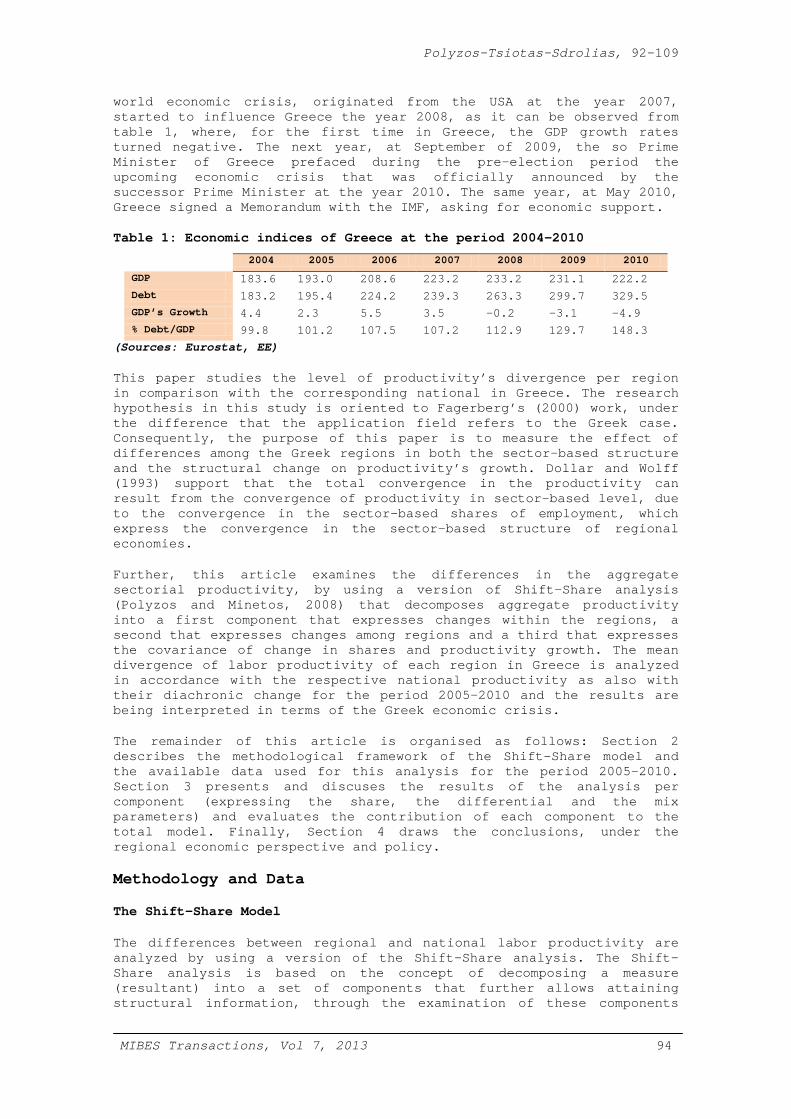
world economic crisis, originated from the USA at the year 2007, started to influence Greece the year 2008, as it can be observed from table 1, where, for the first time in Greece, the GDP growth rates turned negative. The next year, at September of 2009, the so Prime Minister of Greece prefaced during the pre-election period the upcoming economic crisis that was officially announced by the successor Prime Minister at the year 2010. The same year, at May 2010, Greece signed a Memorandum with the IMF, asking for economic support.

Table 1: Economic indices of Greece at the period 2004-2010

2004 2005 2006 2007 2008 2009 2010

GDP 183.6 193.0 208.6 223.2 233.2 231.1 222.2 Debt 183.2 195.4 224.2 239.3 263.3 299.7 329.5 GDP’s Growth 4.4 2.3 5.5 3.5 −0.2 −3.1 −4.9 % Debt/GDP 99.8 101.2 107.5 107.2 112.9 129.7 148.3

(Sources: Eurostat, EE)

This paper studies the level of productivity’s divergence per region in comparison with the corresponding national in Greece. The research hypothesis in this study is oriented to Fagerberg’s (2000) work, under the difference that the application field refers to the Greek case. Consequently, the purpose of this paper is to measure the effect of differences among the Greek regions in both the sector-based structure and the structural change on productivity’s growth. Dollar and Wolff (1993) support that the total convergence in the productivity can result from the convergence of productivity in sector-based level, due to the convergence in the sector-based shares of employment, which express the convergence in the sector-based structure of regional economies.

Further, this article examines the differences in the aggregate sectorial productivity, by using a version of Shift-Share analysis (Polyzos and Minetos, 2008) that decomposes aggregate productivity into a first component that expresses changes within the regions, a second that expresses changes among regions and a third that expresses the covariance of change in shares and productivity growth. The mean divergence of labor productivity of each region in Greece is analyzed in accordance with the respective national productivity as also with their diachronic change for the period 2005-2010 and the results are being interpreted in terms of the Greek economic crisis.

The remainder of this article is organised as follows: Section 2 describes the methodological framework of the Shift-Share model and the available data used for this analysis for the period 2005-2010. Section 3 presents and discuses the results of the analysis per component (expressing the share, the differential and the mix parameters) and evaluates the contribution of each component to the total model. Finally, Section 4 draws the conclusions, under the regional economic perspective and policy.

Methodology and Data

The Shift-Share Model

The differences between regional and national labor productivity are analyzed by using a version of the Shift-Share analysis. The Shift-Share analysis is based on the concept of decomposing a measure (resultant) into a set of components that further allows attaining structural information, through the examination of these components



(Polyzos, 2011). Labor productivity, in a region r and at the time t, can be estimated by using the formula of relation (1), where Pr,t expresses the Productivity in region r, at time t, AV expresses the Added Value and E the Employment, where i stands for the indicator of the Economic Sector in the summation operator.

r,t ri.tr,t

ir,t r,t

AV AVp = =

E E∑ (1)

Relation (1) may be further edited, by using a multiplication treatment, providing the equivalent relation (2).

r,t ri,tri.t ri.tr,t

i ir,t r,t r,t ri,t

AV EAV AVp = = =

E E E E⋅∑ ∑ (2)

For the measures AV and E the expressions of relation (3) stand.

r,t ri.tr

AV = AV∑ , r,t ri.tr

E = E∑ and ri.t

i r

E = E∑ ∑ (3)

Further, relation (2) may provide the equivalent relation (4), after introducing the zero terms ± i,t tE E and ± i.t i,tAV E into its right side.

ri,t ri.tr.t

i r,t ri,t

E AVP

E E

= ⋅ =

∑

ri,t i,t i,t ri.t i.t i.t

i r,t t t ri,t i,t i,t

E E E AV AV AV+ - . + -

E E E E E E

= = ∑

ri,t i,t i,t ri.t i.t i.t

i r,t t t ri,t i,t i,t

E E E AV AV AV- + . - +

E E E E E E

= ∑

(4)

Assuming that:

the ratio ri,t ri,t ri,tAV E = p expresses the labor productivity in region

r, for the sector i, at time t, =r,t r,t r,t rAV E p = p stands for the labor productivity in region r for

the total of sectors, at the time t, ri,t r,t ri,tE E = s expresses the share of employment of sector i, in

region r, at the time t, and i,t t i,tE E = s stands for the share of employment of sector i in the

total employment of the country, at the time t,

then the labor productivity pr, for the region r, can be written as shown in relation (5).

[ ] [ ]r ri ri ri i i ri i ii i

p = s p = (s - s )+ s . (p - p )+ p∑ ∑ (5)

Equation (5) is equivalent to relation (6), given that i ii

s p = p∑ .



( ) ( ) ( ) ( ) ( )r ri i i ri i i ri i ri ri i i

5 p = s - s p + p - p s s - s p - p p⇔ ⋅ ⋅ + ⋅ +∑ ∑ ∑

rp - p =diff A B C⇔ = + +

(6)

where ( )ri i ii

= s - s pA ⋅∑ , ( )ri i ii

B = p - p s⋅∑ and

( ) ( )ri i ri ri

= s - s p pC ⋅ −∑ .

Relation (6) stands for an expression of the Shift-Share model (Polyzos, 2011; Polyzos and Pnevmatikos, 2011), decomposing the divergence of the regional productivity into three components. Further, if diving both sides by p, relation (6) expresses percentage growth rates (Vijselaar and Albers, 2004).

The mathematical formula of the first component ( )ri i ii

= s - s pA ⋅∑

calculates the sum of differences between regional and national shares in employment times the national productivity of each sector, for the total of the sector cases (i=1,2,…,n) and for a certain region r. As a result, this component of productivity share captures the effect of changes that is ought to the sector structure of each region. This term can be allocated in the effect of sector-based regroupings that exhaust the total of sectors.

The second component ( )ri i ii

B = p - p s⋅∑ calculates the sum of

differences between regional and national productivity times the national shares of employment of each sector, for the total of the sector cases (i=1,2,…,n) and for a certain region r. In particular, the factor pri-pi expresses the divergence of labor productivity for the certain sector in the region r in comparison with the national labor productivity for same examined sector.

The second component (B) expresses the effect in productivity caused by the peculiarities of each region and so it is called differential or regional or local-factor effect. According to Fagerberg (2000) the differential component measures the contribution of a regions’ productivity within the individual sector to the overall productivity’s growth and, according to Vijselar and Albers (2004), this component can interpret the counterfactual productivity growth that is free of productive structural changes.

The third component ( ) ( )ri i ri ri

= s - s p pC ⋅ −∑ calculates the sum of

differences among pairs of regional and national shares in employment times the sum of differences between regional and national productivity. This component measures the effect of interactions between the previous two components A and B, that stands for the productivity share and the differential effect and it suggests the covariance of changes in shares and in productivity and concerning the sign of growth in share (positive or negative), which is associated with the productivity growth (dynamic shift effect).

The third component is so called proportionality or mix effect. Fagerberg (2000) observes that this component turns positive when the rapidly developing (in terms of productivity) sectors also increase their share in the total employment and thus it reflects the



capability of a region to redistribute its resources into sectors having greater growth rates.

In relation (6), the two last terms in the right side provide the sum

ri i rii

(p - p )s∑ . Therefore, the divergence of regional to national labor

productivity is further decomposed into a pair of components, due to the mathematic expression of relation (7). As it can be seen in relation (7), the first component A΄is equal to the corresponding first A of relation (6), A=A΄, whereas relation’s (7) second component B΄ embodies the respective two last components B΄=B+C of relation (6).

r ri i i ri i rii i

= p - p = A΄ + B΄ = (s - s )p + (p - p )sdiff ∑ ∑ (7)

Component B΄ in relation (7) calculates the sum of differences between regional and national productivity times the regional shares of employment of each sector, for the total of the sector cases (i=1,2,…,n) and for a certain region r and thus it expresses the contribution of a regions’ productivity within the individual sector to, this time, the regional productivity’s growth. In other words, this component expresses the differentiation in the employment shares of one region that it is caused by this region’s productivity specialization.

Data

The available data in this study concern the variables of regional Employment (E), measured in number of thousand working people, and of the Gross Added Value (AV), measured in million Euros, in Greece. The data refer to records per Greek region and productivity sector for the six-year period 2005-2010. All Greek regions and productivity sectors considered in this study are presented in Table 2.

Table 2: Regions and Productivity Sectors that are considered in the analysis

CODE REGION CODE PRODUCTIVE SECTOR

R1 East Macedonia i=1 Agriculture, forestry and fishing

and Thrace i=2 Mining and quarrying, manufacturing,

R2 Central Macedonia electricity, gas, steam, air conditioning

R3 West Macedonia and water supply, sewerage, waste management

R5 Epirus and remediation activities

R6 Ionian Islands i=3 Construction

R7 West Greece i=4 Wholesale and retail trade, repair of motor

R8 Central Greece vehicles and motorcycles, transportation and

R9 Peloponnese storage, accommodation and food service

R10 Attica activities

R11 North Aegean i=5 Information and communication

R12 South Aegean i=6 Financial and insurance activities

R13 Crete i=7 Real estate activities

i=8 Professional, scientific and technical activities, administrative and support service activities

i=9 Public administration and defense, compulsory social security, education, human health and social work activities

i=10 Arts, entertainment, recreation, other service activities, activities of households as employers, undifferentiated goods and services producing activities of households for own use, activities of extraterritorial organizations and bodies

http://en.wikipedia.org/wiki/Central_Macedonia�

http://en.wikipedia.org/wiki/West_Macedonia�

http://en.wikipedia.org/wiki/Epirus_%28region%29�

http://en.wikipedia.org/wiki/Ionian_Islands_%28region%29�

http://en.wikipedia.org/wiki/West_Greece�

http://en.wikipedia.org/wiki/Central_Greece_%28region%29�

http://en.wikipedia.org/wiki/Peloponnese_%28region%29�

http://en.wikipedia.org/wiki/Attica_%28region%29�

http://en.wikipedia.org/wiki/North_Aegean�

http://en.wikipedia.org/wiki/South_Aegean�

http://en.wikipedia.org/wiki/Crete�



Results and Discussion

The Shift-Share analysis, applied in this paper, is based on the 3-component model described by relation (6) and on the 2-component model of relation (7). The changes in the regional productivity diff=pr-p are decomposed into three components, the productivity share, the differential effect and the mix effects component. The results of the analysis are shown in table 3, for the six-year period 2005-2010.

Table 3: Results of the Shift-Share analysis Year

RESULTANT (PRODUCTIVITY

DIFFERENCES)

Region 2005 2006 2007 2008 2009 2010 R1 -4621 -4709 -4775 -4833 -4803 -4679 R2 -4619 -4707 -4773 -4831 -4801 -4678 R3 -4609 -4698 -4764 -4822 -4793 -4669 R4 -4620 -4707 -4775 -4833 -4803 -4681 R5 -4620 -4709 -4776 -4835 -4806 -4682 R6 -4615 -4700 -4766 -4827 -4798 -4675 R7 -4620 -4707 -4775 -4833 -4805 -4682 R8 -4613 -4702 -4768 -4826 -4796 -4673 R9 -4620 -4707 -4774 -4834 -4804 -4679 R10 -4605 -4691 -4756 -4814 -4783 -4659 R11 -4616 -4703 -4770 -4825 -4796 -4674 R12 -4605 -4690 -4757 -4814 -4783 -4660 R13 -4618 -4705 -4772 -4829 -4799 -4675

COMPONENT A

(PRODUCTIVITY SHARE)

2005 2006 2007 2008 2009 2010 R1 -4618 -4706 -4772 -4830 -4800 -4676 R2 -4612 -4699 -4765 -4823 -4793 -4669

R3 -4616 -4703 -4770 -4828 -4799 -4673 R4 -4615 -4702 -4768 -4827 -4796 -4674 R5 -4617 -4705 -4772 -4830 -4801 -4677 R6 -4611 -4697 -4763 -4822 -4793 -4671 R7 -4618 -4705 -4771 -4829 -4800 -4677 R8 -4611 -4698 -4765 -4823 -4792 -4669 R9 -4619 -4707 -4774 -4833 -4803 -4679 R10 -4610 -4696 -4762 -4820 -4789 -4666 R11 -4616 -4703 -4769 -4825 -4794 -4672 R12 -4614 -4701 -4768 -4825 -4796 -4672 R13 -4615 -4702 -4767 -4823 -4795 -4674

COMPONENT B (DIFFERENTIAL

EFFECT)

Reg. 2005 2006 2007 2008 2009 2010 R1 -282 -415 -385 -455 -417 -409 R2 -427 -545 -439 -435 -441 -530

R3 638 292 399 306 -33 -196 R4 -260 -221 -288 -346 -389 -519 R5 -483 -744 -673 -854 -853 -842 R6 443 574 534 241 25 -103 R7 -381 -445 -570 -643 -806 -818 R8 252 -24 -54 63 83 4 R9 -208 -218 -365 -402 -361 -409 R10 968 1059 1366 785 763 1015 R11 -55 57 -138 7 40 -111 R12 1105 1549 1225 1313 1552 1527 R13 -214 -146 -249 -115 30 169

COMPONENT C (MIX EFFECT) Reg. 2005 2006 2007 2008 2009 2010

R1 279 412 383 452 414 407 R2 420 537 432 427 433 521

R3 -631 -287 -393 -299 38 200 R4 255 216 281 340 382 512 R5 481 740 669 849 848 837 R6 -447 -578 -538 -246 -31 100 R7 379 443 567 640 801 813 R8 -254 21 50 -66 -87 -7 R9 207 218 364 401 361 409 R10 -963 -1054 -1360 -778 -756 -1008 R11 55 -57 137 -8 -42 108 R12 -1097 -1539 -1215 -1302 -1539 -1515 R13 210 143 244 110 -34 -170



As it can be observed from table 3, all values of the productivity’s changes (diff=pr-p) in Greece are negative, indicating that, in the total of cases, the national productivity in Greece outperforms the corresponding regional. This observation may imply that none of the Greek regions posses a core role so as to determine the total productivity of the country or, alternatively, that the national level of productivity in Greece is being generated through an additive process, where all the Greek regions contribute in a cooperative way, in order to produce a higher national result. It is probably noteworthy that even in the case of Attica, which is the region having almost the half population of the country (Polyzos and Tsiotas, 2012), the regional productivity is not sufficient to overcome the corresponding national value.

Map and Graphical Results

The results of table 3 are further illustrated at the maps of figure 1, where each map represents the annual state of the Shift-Share components per Greek region, for the six-year period 2005-2010. The right map of figure 1 illustrates the productivity values of table 3, after being normalized by the respective Greek regional population of the year 2006.

Figure 1: Left: Annual results of the Shift-Share terms (shown in colors) per Greek region, for the period 2005-2010. Right: The same map with normalized values by population (darkest region represent greatest differences in productivity).

Both maps of figure 1 indicate that the contribution of the productivity share (component A) seems to be the most determinative component to the divergence (differences) of the regional productivity (diff=pri-pi). These Shift-Share terms (diff, comp.A) also seem to have their values similarly distributed. The contribution of the rest pair of components (B and C) to the Shift-Share model seems to be negligible, since values appear to be anti-symmetric and thus the pair sum should be probably neutralized. The validity of these observations is being statistically tested in a following paragraph.

Additionally, the map with the normalized values of figure 1 (right) elects these Greek regions that present the greatest differences in productivity, in comparison with the respective national level. As it can be observed from this map, the borderline or distant Greek regions



present greater productivity differences, fact that it may be related to distance and thus to transportation matters. According to the information of this map, the regions of Attica (1) and of Central Macedonia (2) present the strongest productivity picture and, on the other hand, the regions of West Macedonia (3), Epirus (5), Ionian Islands (6), North Aegean (11) and of South (12) Aegean present the weakest picture.

For a further graphical assessment, the diagrams of figure 2 showing the diachronic fluctuation per Greek region of the Shift-Share terms are constructed, for the period 2005-2010. These diagrams are chosen to be presented in pairs (diff,A) and (B,C), due to the obvious relevance of these pair components. The first pair-diagram (left), first of all, spots the previously detected similarity, between the term of productivity differences (diff=pr-p) and of component A (productivity share). This pair-diagram also indicates the existence of an inconsiderable variability in the interregional fluctuations of these Shift-Share terms (diff, comp.A), which is illustrated by the dense position of their U-shaped diagrams. This observation also implies the existence of an interregional homogeneity for the Shift-Share terms diff and component A.

Figure 2: Diagrams showing the diachronic fluctuations of the Shift-Share pairs (diff=pri-pi, comp.A) (left) and (comp.B, comp.C) (right), per Greek region (r=1,..,13).



On the other hand, the second pair-diagram (right) of figure 2, consisting of the Shift-Share components B and C, presents a considerable interregional variability. The contribution of this component pair to the model may be considered latent, under the unified aspect B΄=B+C of relation (7), whether taking under consideration their anti-symmetric values that were previously observed. Nevertheless, the pair consideration of these components, despite the fact that it seems not to contribute significantly to the model, illustrates a bipolar performance that its study is of certain interest in Regional Science.

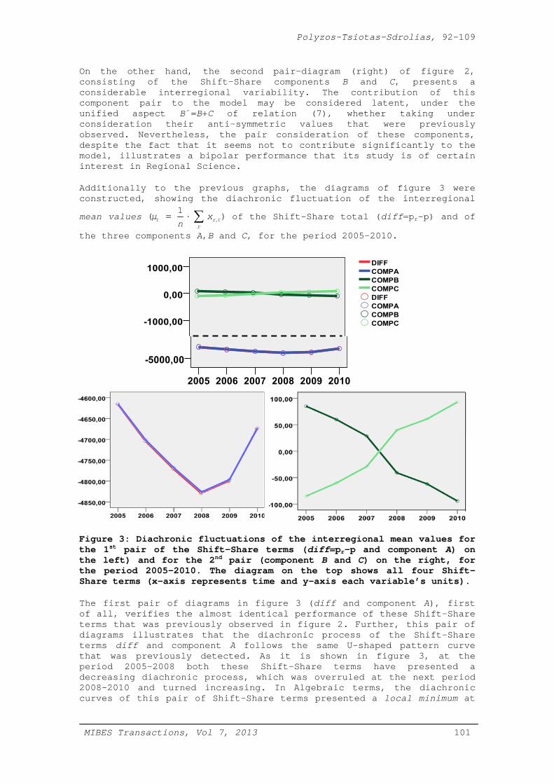
Additionally to the previous graphs, the diagrams of figure 3 were constructed, showing the diachronic fluctuation of the interregional

mean values ,

1( )t r t

r

μ xn

= ⋅ ∑ of the Shift-Share total (diff=pr-p) and of

the three components A,B and C, for the period 2005-2010.

Figure 3: Diachronic fluctuations of the interregional mean values for the 1st pair of the Shift-Share terms (diff=pr-p and component A) on the left) and for the 2nd pair (component B and C) on the right, for the period 2005-2010. The diagram on the top shows all four Shift-Share terms (x-axis represents time and y-axis each variable’s units).

The first pair of diagrams in figure 3 (diff and component A), first of all, verifies the almost identical performance of these Shift-Share terms that was previously observed in figure 2. Further, this pair of diagrams illustrates that the diachronic process of the Shift-Share terms diff and component A follows the same U-shaped pattern curve that was previously detected. As it is shown in figure 3, at the period 2005-2008 both these Shift-Share terms have presented a decreasing diachronic process, which was overruled at the next period 2008-2010 and turned increasing. In Algebraic terms, the diachronic curves of this pair of Shift-Share terms presented a local minimum at



the year 2008, for the period 2005-2010, following a decreasing process the period before and increasing one the period after.

Moreover, whether interpreting this observation in conjunction with the fact that Greece started to be influenced by the world economic crisis at the year 2008, then the increasing overturn in both the productivity differences (diff=pr-p) and the regional productivity share (component A) comes to an agreement with the theoretical background saying that regional inequalities (Tsiotas and Polyzos, 2011; Tsiotas and Polyzos, 2013) converge during the periods of economic crisis (Petrakos and Psicharis, 2004; Polyzos, 2011).

The second pair of diagrams (components B and C) in figure 3 verifies the anti-symmetric performance of the Shift-Share components B and C (local and proportionality effect). The diachronic process of component B is presented to be decreasing at the period 2005-2010 and the respective of component C increasing. The decreasing curve of component B indicates that the local specialization of the Greek regions weakens through time.

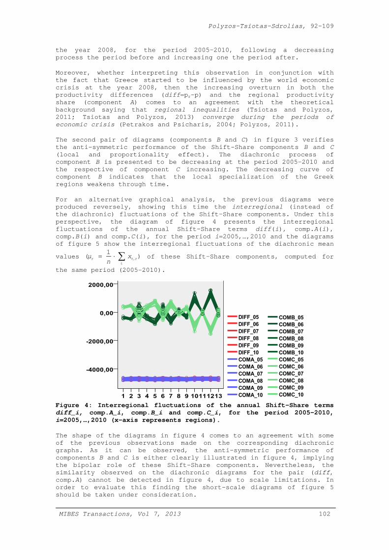
For an alternative graphical analysis, the previous diagrams were produced reversely, showing this time the interregional (instead of the diachronic) fluctuations of the Shift-Share components. Under this perspective, the diagram of figure 4 presents the interregional fluctuations of the annual Shift-Share terms diff(i), comp.A(i), comp.B(i) and comp.C(i), for the period i=2005,…,2010 and the diagrams of figure 5 show the interregional fluctuations of the diachronic mean

values ,

1( )r t r

t

μ xn

= ⋅ ∑ of these Shift-Share components, computed for

the same period (2005-2010).

Figure 4: Interregional fluctuations of the annual Shift-Share terms diff_i, comp.A_i, comp.B_i and comp.C_i, for the period 2005-2010, i=2005,…,2010 (x-axis represents regions).

The shape of the diagrams in figure 4 comes to an agreement with some of the previous observations made on the corresponding diachronic graphs. As it can be observed, the anti-symmetric performance of components B and C is either clearly illustrated in figure 4, implying the bipolar role of these Shift-Share components. Nevertheless, the similarity observed on the diachronic diagrams for the pair (diff, comp.A) cannot be detected in figure 4, due to scale limitations. In order to evaluate this finding the short-scale diagrams of figure 5 should be taken under consideration.



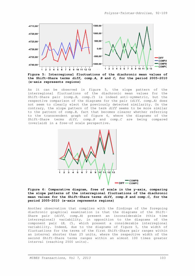
Figure 5: Interregional fluctuations of the diachronic mean values of the Shift-Share terms diff, comp.A, B and C, for the period 2005-2010 (x-axis represents regions)

As it can be observed in figure 5, the slope pattern of the interregional fluctuations of the diachronic mean values for the Shift-Share pair (comp.B, comp.C) is indeed anti-symmetric, but the respective comparison of the diagrams for the pair (diff, comp.A) does not seem to clearly elect the previously detected similarity. On the contrary, the slope pattern of the term diff seems to be more similar to the pattern of comp.B, fact that becomes clearer whether referring to the transcendent graph of figure 6, where the diagrams of the Shift-Share terms diff, comp.B and comp.C are being compared (overlaid) in a free-of scale perspective.

Figure 6: Comparative diagram, free of scale in the y-axis, comparing the slope patterns of the interregional fluctuations of the diachronic mean values for the Shift-Share terms diff, comp.B and comp.C, for the period 2005-2010 (x-axis represents regions)

Another observation that complies with the findings of the foregoing diachronic graphical examination is that the diagrams of the Shift-Share pair (diff, comp.A) present an inconsiderable (this time interregional) variability, in opposition to the diagrams of the component pair (B, C), which present a considerable interregional variability. Indeed, due to the diagrams of figure 5, the width of fluctuations for the terms of the first Shift-Share pair ranges within an interval shorter than 25 units, where the respective width of the second Shift-Share terms ranges within an almost 100 times greater interval (reaching 2500 units).



The foregoing bi-partial (both diachronic and interregional) graphical consideration let us shape the impression that in the case of the Greek regional productivity the Shift-Share model is mainly controlled by the presence of the component A, since the anti-symmetric components B and C seem to be mutually neutralized. In terms of mean (interregional or diachronic) values, the Shift-Share model leaves the impression that the precision of the model depends on the reference variable used each time (time or regional unit) and thus that the Shift-Share model is vulnerable to transformations. This impression seems to come to a contrary to the assumption that the Shift-Share framework suggests a conservative and thus transformation-free environment, in terms of Physics (Serway, 1990), under the consideration that the Shift-Share model constitutes a decomposition process where quantities are preserved.

Nevertheless, the previous contrary seems not to suggest a concern, whether arranging the results of the foregoing examination. In terms of scale, all previous comparative graphs indicate that the arithmetic value of the Shift-Share term diff is controlled almost absolutely by component A. This result can be easily evaluated whether producing the tables of differences diff-comp.A, diff-comp.B and diff-(-comp.C), where their absolute values range respectively within the intervals [0,13], [3840,6335] and [3846,6322]. Obviously, the length of the first interval [0,13] is inconsiderable, in comparison with the respective other two lengths, implying that the Shift-Share terms diff and comp.A are almost of the same quantities. On the other hand, in terms of slope patterns of the curves, the previous graphs indicate that the slope pattern of the Shift-Share model seems to be controlled by the pattern of comp.A (productivity share) in the diachronic case and by the pattern of comp.B (local effect) in the interregional case. These observations are being tested at the following paragraph.

Statistical Testing

For quantifying and evaluating the findings of the foregoing graphical examination of the Shift-Share analysis, a statistical treatment is next being applied. The statistical tools used for the testing are the Pearson’s coefficient of linear bivariate correlation and the linear regression model. The main concept of the analysis is based on considering the term of the productivity differences (diff=pr-p) as the dependent or response variable and examining whether the rest three Shift-Share components (possessing the role of independent or predictor variables) are related to the response variable and in which extent.

The Pearson’s bivariate linear coefficients of correlation (Norusis, 2004; Devore and Berk, 2012) are calculated in order to detect the existence of linear relations among pairs of variables consisting of the Shift-Share terms. The mathematical formula of the Pearson’s bivariate linear coefficient of correlation is shown at relation (1), where cov(x,y)≡sxy stands for the covariance (Devore and Berk, 2012) of

variables x,y and var( ) xx s≡ , var( ) yy s≡ are their respective

standard deviations (Damianou, 2003; Devore and Berk, 2012).

≡ = ≡ ⋅⋅

cov( , )( , ) ( )

var( ) var( )xy xy x y

x yr x y r s s s

x y (8)

Table 4 shows the correlation results in pairs of the Shift-Share model (relation 6). The auxiliary index “_R” or “_Y” at the end of the



variable names indicate whether the mean values are calculated among regions or years, in correspondence. All correlation results in this table are significant (sig.<0,05) implying that the possibility the recorded correlation value to result by a chance is less than 5%.

Table 4: Correlation analysis results

N Coef. Correlation Sig.

Pair 1 DIFF_R & COMPA_R 6 1.000 0.000

Pair 2 COMPB_R & COMPC_R 6 -1.000 0.000

Pair 3 DIFF_Y & COMPA_Y 13 0.616 0.025

Pair 4 DIFF_Y & COMPB_Y 13 0.968 0.000

Pair 5 COMPB_Y & COMPC_Y 13 -1.000 0.000

The results of table 4 evaluate the foregoing graphic consideration referring to the slope pattern of the Shift-Share terms. As it is shown in this table, the first pair of variables is perfectly (strong and significanlty) linearly correlated, implying that, in the diachronic case (N=6), the slope pattern of the Shift-Share term diff is indeed controlled by the slope pattern of comp.A (productivity share). Next, the very strong and significant correlation of the pair 4 in comparison with the just considerable and significant correlation of the pair 3 evaluates the foregoing observation that, in the interregional case (N=13), the slope pattern of the Shift-Share term diff is controlled by the slope pattern of comp.B (local effect). Finally, the correlation results of the pairs 1 and 5 in table 4 (absolutely linear and significant) verify the anti-symmetric performance of the components B and C and thus let us interpreting their role as a dipole.

Continuing, the linear regression analysis (Norusis, 2004; Norusis, 2005) produces an estimation of a linear equation that best describes the relation between the dependent (response) variable and the set of independent (predictors). The optimization criterion that is applied here is the method of Least Squares, where the sum of distances among pairs of estimated and observed values are required to be the minimum. The linear regression algorithm used in this study is the Enter method, where all inserted variables are calculated in the model excluding only these that present significant collinearity. The Enter model in this analysis was requested not to calculate a constant variable, due to the conservative structure of the Shift-Share model.

The results of the linear regression analysis are presented at table 5, for the diachronic (model 1) and the interregional (model 2) cases.

Table 5: Linear regression analysis results

Model 1: Diachronic case (N=6)

Model R R Square Adjusted R

Square Std. Error of the Estimate 1 1.000a 1.000 1.000 .529

a. Predictors: COMPC_R, COMPA_R b. Dependent Variable: DIFF c. Tolerance= .000 limits reached

Model

Unstandardized Coefficients

Standardized Coefficients

t Sig. B St.Error Beta 1 COMPA_R 1.000 .003 1.000 21837.978 .000

COMPC_R -.006 .003 .000 -1.690 .166



Model 2: Interregional case (N=13)

Model R R Square Adjusted R

Square Std. Error of the Estimate 2 1.000a 1.000 1.000 3.10158

a. Predictors: COMPC_Y, COMPA_Y b. Dependent Variable: DIFF_Y c. Tolerance= .000 limits reached

Model

Unstandardized Coefficients

Standardized Coefficients

t Sig. B St.Error Beta 2 COMPA_Y 1.000 .000 1.000 5499.792 .000

COMPC_Y -.008 .001 .000 -5.123 .000

As it can be observed from table 5, both models present absolute fitting ability (Ri2=1, i=1,2), indicating the existence of an absolute linearity for both the diachronic (N=6) and the interregional (N=13) cases. This seemingly comes to a contrary with the previous correlation results presented at table 4. Nevertheless, whether taking under consideration that at the construction part of the model it is requested the algorithms not to calculate constant variables, then it is rationale for these models not to describe the slope fitness ability but the contribution of the Shift-Share components to the summation process.

Additionally, the exclusion of the variable COMPC from both the Enter models indicates the existence of collinearity effects in the Shift-Share structure, verifying the correctness of the pairwise treatment of the Shift-Share components B and C in the graphical examination part. Furthermore, the exclusion of the component B from the linear regression models allows to these regression models to refer to the Shift-Share model of relation (7) and thus to describe the

contribution of the bipolar term ri i rii

(p - p )s∑ , which is according to

table 5 zero.

Evaluating the results in terms of the Greek Economic crisis

The previous inferential statistical analysis, with the use of the linear regression model, allows applying a structural assessment to the decomposition of the regional productivity changes (diff=pr-p), for the period 2005-2010. The almost absolute contribution of the productivity share component (A) to the model, for both diachronic and interregional cases, implies that the shift in one region’s total productivity from the respective national is ought to the pair of differences between regional and national employment ri i(s - s ), considered for the total of the sector cases.

This remark seems rational if comparing the summation products of all the Shift-Share components, where it is observed that only in component A the productivity factor appears in its entire form (·pi), since in all the other cases it concerns differences (pri-pi or pri-pr). In economic terms, this almost absolute contribution interprets that the effect of changes that is ought to the sector structure of each region determine the amount of deviation in one region’s productivity from the respective national.

This observation may attain an interpretation in terms of the Greek economic crisis, which for many academics and politicians is considered as a systemic crisis of the European bank system, under the consideration of the previous statement that regional inequalities



converge during the periods of economic crisis. This convergence in the regional inequalities may operate as a compression mechanism to the endogenous trends, which tries to differentiate the productivity dynamics of a region resulting to the weakening of its local specialization performance.

Additionally, the decreasing diachronic process in the diagram of Shift-Share component B, shown in figure 3, does not seem to present a considerable variability in the year 2008, where Greece started to be influenced by the previous worldwide, probably due to the existence of a pre-crisis period that may cover the diachronic range of 2005-2008. Such an assertion may be rational, whether considering that Greece faced a considerable deflation in the economic sector of constructions at the meta-Olympic Games (Athens 2004) period.

On the other hand, the increasing diachronic process in the diagram of the third Shift-Share component (C), in figure 3, implies according to Fagerberg (2000) the existence of rapidly developing (in terms of productivity) sectors that increase their share in the total employment and thus reflecting the capability of some regions to redistribute their resources into sectors that have greater growth rates. This assertion may imply that the meta-Olympic period in Greece favored the redistribution of the regional productivity into these sectors having high national growth rates and thus not to these electing the local specialization dynamics.

Finally, given that the contribution of the second and the third component is pairwise negligible, it may be asserted that the loss in the local specialization was resonated with the proportionality effect in a way that the productivity effects to be mutually retracted. A considerable perhaps point in the diachronic process of this pair of curves (B and C), in figure 3, is the intersection point of these curves, located in the middle of the year 2007-2008, where the interregional mean values of the components B and C are zero.

Conclusions

This paper studied the differences of regional productivity in Greece, by using a version of the Shift-Share analysis and by evaluating graphically and statistically the results produced by the Shift-Share model. The available data concerned records on regional productivity, on added value and labor employment, per economic sector, for the period 2005-2010. The analysis was based on the decomposition attribute of the Shift-Share model, targeting to illustrate a structural picture of the Greek regional productivity, through the examination of each Shift-Share decomposition component.

One primary outcome of the foregoing Shift-Share analysis indicated that none of the Greek regions, not even Attica, occupies a central role so as to overstep the national rates in productivity and thus to determine the evolutionary patterns of productivity, at the scale of the country. This result implies that the national level of productivity in Greece operates additively, having all the regions to contribute positively into the national total.

At the decomposition part of the Shift-Share analysis it was elected that the contribution of the first component (productivity share) seems to be the most determinative to the model, where the presence of the second and the third components is mutually neutralized, producing latent results. The almost absolute contribution of the first



component to the model implies that the differences in regional productivity, from the respective national, are ought to the differences in employment ri i(s - s ), fact that sets the labor and consequently the social capital as the most significant determinative factors in the productivity map of the country.

Additionally, the second and the third components of the Shift-Share model presented an intense interregional variability in their diachronic (2005-2010) process. The case regarding the second component implies that the interregional productivity pattern in Greece is described by a considerable heterogeneity and thus by a local specialization, which is, unfortunately, eventually sharpened. In the case of the third component, the interregional variability implies the existence of a heterogeneous pattern describing different capability rates of the regions to redistribute their resources into sectors having greater growth rates.

Finally, the diachronic range of the available dataset allowed interpreting the results of the foregoing Shift-Share analysis in terms of the most significant recent events in the Greek economic History, such as are the meta-Olympic Games (Athens 2004) period and the forerunner period of the economic crisis, which was formally announced at the pre-election period in Greece at the fall of 2009. Consequently, it is obvious that the previous modern-economic historical events have let their imprints on the productivity foundation of Greece. The regional productivity differences moved decreasing after the year 2004, implying an uneven regional allocation of the dynamics in productivity, where the sudden increasing turnover in productivity differences at the year 2008, were the economy of Greece started to be influenced by the previous worldwide economic crisis, imply a convergence in regional inequalities, fact which comes to an agreement with the Regional theory.

References

Alam, A., Casero, P., Khan, F., Udomsaph, C., (2008) “Unleashing Prosperity Productivity Growth in Eastern Europe and the Former Soviet Union”, The International Bank for Reconstruction and Development/The World Bank, Washington.

Baumol, W., Batey-Blackman, SA., Wolff, E., (1989), “Productivity and American Leadership: the Long View”, The Cambridge Massachusetts, MIT Press.

Burruss, G., Bray, T., (2005) “Confidence Intervals”, Encyclopedia of Social Measurement, 1, pp.455-462.

Damianou, C., (2003) An introduction to Statistics, Part Ι, Athens, Greece, Symmetria Publications [in Greek].

Devore, J., Berk, K., (2012) Modern Mathematical Statistics with Applications, London, UK, Springer-Verlag Publications.

Fagerberg, J., (2000) “Technological progress, structural change and productivity growth: a comparative study”, Structural Change and Economic Dynamics, 11(4), pp.393-411.

Norusis, M., (2004) SPSS 13, Advanced statistical procedures companion, New Jersey (USA), Prentice Hall Publications.

Norusis, M., (2005) SPSS 14.0 Statistical Procedures Companion, New Jersey (USA), Prentice Hall Publications.

Petrakos, P., Psicharis, G., (2008) Regional Development in Greece, Athens, Greece, Kritiki Publications [in Greek].

Polyzos S., Minetos D., (2008) “Structural Change and the Productivity Growth in Greek Regions”, Proceedings of 4th International Conference of ASECU on Development Cooperation and

http://ideas.repec.org/s/eee/streco.html�





Competitiveness, Bucharest Academy of Economic Studies, May 2008, Bucharest, Romania, pp.462-473.

Polyzos, S., (2011) Regional Development, Athens, Greece, Kritiki Publications [in Greek].

Polyzos, S., Minetos, D., Sdrolias, L. (2007) “Productivity and spatial diffusion of technology in Greece: An empirical analysis”, Journal of International Business and Economy, 8(1), pp.105-123.

Polyzos, S., Pnevmatikos, T., (2011) “Evaluation of Regional Inequalities in Greece by Using Shift-Share Analysis”, International Journal of Engineering and Management, 3(2), pp. 119-131.

Polyzos, S., Sofios, S., (2008) “Regional multipliers, Inequalities and Planning in Greece”, South Eastern Europe Journal of Economics, 6(1), pp.75-100.

Polyzos, S., Tsiotas, D., (2012) “The Evolution and Spatial Dynamics of Coastal Cities in Greece”, in Polyzos, S., (2012) (ed) Urban Development, Croatia, Intech Publications, pp.275-296. (ISBN: 978-953-51-0442-1)

Tsiotas, D., Polyzos, S., (2011) “Introducing an inequalities index from the simple perceptron pattern in ANN: an unemployment inequalities application in Regional Economics, Journal of Engineering Science and Technology Review, 4(3), 291-296.

Tsiotas, D., Polyzos, S., (2013) “The contribution of ANN’s simple perceptron pattern to inequalities measurement in Regional Science”, Operational Research an International Journal, 13(2), 289-301.

Serway, R., (1990) Physics for Scientists & Engineers, Volume Ι, London, Saunders College Publishing, Third Edition.

Vijselaar, F., Albers, R., (2004) “New Technologies and Productivity Growth in the Euro Area”, Empirical Economics, 29, pp.621-646.

greek regional productivity at the period of the economic ... · the economic crisis: obtaining...

Documents