Gravity Models of the Intra-EU Trade: Application ofthe Hausman-Taylor Estimation in HeterogeneousPanels with Common Time-specific Factors∗

Laura SerlengaSchool of Economics, University of Edinburgh

Yongcheol ShinSchool of Economics, University of Edinburgh

February 2004

Abstract

In this paper we follow recent developments of panel data studies and explicitlyallow for the existence of unobserved common time-specific factors where their indi-vidual responses are also allowed to be heterogeneous across cross section units. Inthe context of this extended panel data framework we generalize the Hausman-Taylorestimation methodology and develop the associated econometric theory. We apply ourproposed estimation technique along with the conventional panel data approaches toa comprehensive analysis of the gravity equation of bilateral trade flows amongst the15 European countries over 1960-2001. Empirical results clearly demonstrate that ourproposed approach fits the data reasonably well and provides much more sensible re-sults than the conventional approach based on the fixed time dummies. These findingsmay highlight the importance of allowing for a certain degree of cross section depen-dence through unobserved heterogeneous time specific common effects, otherwise theresulting estimates would be severely biased.

JEL Classification: C33, F14.Key Words: Gravity Models of Trade, Heterogeneous Panel Data, Hausman-Taylor Es-

timation, Time-specific Common Factors, Intra-EU Trade.

∗We are grateful to Colin Roberts, Ron Smith, Andy Snell and seminar participants at University ofEdinburgh for their helpful comments. The usual disclaimer applies.

1 Introduction

The gravity model of international trade flows has been widely used as a baseline model forestimating the impact of a variety of policy issues related to regional trading groups, currencyunions and various trade distortions, e.g. Bougheas, Demetriades and Morgenroth (1999), DeGrauwe and Skudelny (2000), Glink and Rose (2002), Martinez-Zaroso and Nowak-Lehmann(2003) and De Sousa and Disdier (2002). Since the seminal paper by Anderson (1979), someattempts have also been made explicitly to derive the prediction of the gravity model fromdifferent theoretical models such as Ricardian models, Heckscher-Olin models and IncreasingReturns to Scale models, e.g. Bergstrand (1990), Markusen and Wigle (1990) and Leamer(1992). As argued by Davis (2000), it is nowadays remarkable to observe that in the spaceof a little more than a decade the gravity model has gone from theoretical orphan to havingseveral competing claims to maternity.Recently, it is criticised that the use of conventional cross-section estimation is misspec-

ified since it is not able to deal with bilateral (exporter and/or importer) heterogeneity,which is extremely likely to be present in bilateral trade flows. In this regard a panel-based approach will be desired because heterogeneity issues can be modelled by includingcountry-pair “individual” effects. In particular, Matyas (1997) argues that the correct econo-metric specification should be the so-called “triple-way model”, where time, exporter andimporter effects are specified as fixed and unobservable. But, Egger and Pfaffermayr (2002)demonstrate that when the Matays’ triple-way model is extended to include bilateral tradeinteraction effects, then this three-way specification reduces to a conventional two-way modelwith time and bilateral effects only. Although a number of panel estimation techniques suchas the pooled OLS, the Fixed Effects Model, the Random Effects Model have been appliedin various contexts, the assumption that unobserved individual effects are uncorrelated withall the regressors is convincingly rejected in almost all studies. Therefore, the Fixed Effectsestimation has been the most preferred estimation method in order to avoid the potentiallybiased estimation, e.g. Cheng and Wall (2002).However, it is worth noting that the Fixed Effects approach does not allow for estimat-

ing coefficients on time invariant variables such as distance or common language dummies,though the consistent estimation of such effects are equally important in many situations.Cheng and Wall (2002) simply suggest to estimate the regression of the (estimated) individ-ual effects on individual-specific variables by the OLS, though this approach clearly ignoresthe potential correlation between individual specific variables and (unobserved) individualeffects such that the resulting estimates are likely to be severely biased. In order to properlyaddress this issue we need to employ the Hausman and Taylor (1981, hereafter HT) instru-mental variable estimation technique, see for example Brun, Carrere, Guillaumont and deMelo (2002) for the HT estimation of gravity models of international trade. Most recentempirical studies also emphasise the importance of explicitly allowing for the presence oftime specific effects in order to capture business cycle effects or to deal with globalizationissues. The conventional approach extends the benchmark model simply by incorporatingthe fixed T − 1 time dummies in the panel regression, e.g. Matyas (1997), De Sousa andDisdier (2002) and Egger (2002).In this paper we follow recent developments of panel data studies surrounding the use

[1]

of unobserved common time effects, e.g. Ahn, Lee and Schmidt (2001), Bai and Ng (2002),Pesaran (2002) and Phillips and Sul (2002), and advance an alternative estimation frame-work in which we explicitly allow for the existence of observed and/or unobserved commontime-specific factors and also allow the individual responses to those common factors to beheterogeneous across country pairs. This approach has an additional advantage in accom-modating certain degrees of cross section dependence through heterogeneous time-specificfactors, in which case we may avoid the potential bias of the uncorrected estimates. In par-ticular, we aim to generalize the HT estimation in this extended panel data setup, developthe underlying econometric theory but also propose an alternative source of instruments inaddition to the (internal) instruments suggested by HT; namely, some of (consistently es-timated) heterogeneous time-specific factors under the assumption that they are correlatedwith individual specific variables but not with unobserved individual effects.We apply our proposed HT estimation technique along with the conventional panel data

approaches to a comprehensive analysis of the sources of bilateral trade amongst the 15European countries over 1960-2001. We use both the triple and the double indexed versionsof the gravity equation, where we consider as the dependent variable the logarithm of realexport in the former and the logarithm of total trade in the latter. First, we use thebasic specification and consider the impacts of core explanatory variables such as GDP andpopulation, and the distance. We then augment the basic specification by adding variousvariables such as common language, common border, free trade area and currency unionmembership dummies. Finally, we follow recent theoretical developments [e.g. Helpman(1987) and Egger (2002)] and include variables measuring both similarity in relative size oftrading countries and differences in relative factor endowments.Our main empirical findings are summarised below. First, the impact of the GDP vari-

ables is always significantly positive, whereas the impact of population variables is found tobe mostly insignificant. Second, the impacts of free custom union membership are all posi-tively significant, whilst the results are mixed for the impacts of EMU . Third, the impactof similarity in relative size of trading countries are mostly significant and positive, whilethe impact of differences in relative factor endowments (RLF ) are somewhat ambiguous.Turning to the estimation results for individual specific variables, the impacts of distance,common language dummy and common border dummy are mostly significantly negative, pos-itive and positive, respectively, as expected. A notable finding is that once the correlationbetween the common language dummy and unobserved individual effect is accommodatedby the HT estimation, there is evidence that the effects of the variables that may proxy forgeographical distance, i.e. distance and common border dummy, might be compensated eachother, whereas the role of cultural affinities proxied by common language dummy becomesmore significant. On the other hand, when using the conventional approach using the T − 1fixed time dummies, the HT estimates of the impact of distance are surprisingly positive butinsignificant, the impacts of common language dummy are significant but seem to be toolarge, and common border dummy loses its statistical significance. This observation mayreflect the practical importance of properly incorporating the time-specific effects.Furthermore, we find that our proposed HT estimation results produce more sensible

predictions on the impacts of differences in factor endowments and of the common currencydummy on intra-EU trade flows than the conventional approach; namely the impacts of both

[2]

EMU and RLF are found to be convincilngly insignificant only in the extended HT model.First, considering that the total trade flows are the sum of inter- and intra-industry trades,and RLF is positively correlated only with the intra-industry trade, we may argue that theimpact of RLF on total trade flows would not be unambiguous. Secondly, empirical evidenceon the impact of EMU on trade flows has been at most mixed in the literature, see Rose(2002) and Glink and Rose (2002) for a rather large positive effect of currency union ontrade, and Persson (2001), Pakko and Wall (2002) and De Nardis and Vicarelli (2003) for itsnegative or insignificant effects on trade. In particular, as argued by de Souza (2002), the(evaluation) periods are too short after an introduction of the Euro to use the EMU dummyas an adequate proxy for monetary union membership and therefore, we also expect that theimpacts of EMU are yet to be significantly materialised. This observation may indicate theimportance of properly accommodating a certain degree of cross section dependence throughunobserved heterogeneous time effects, otherwise the resulting estimates would be severelybiased.The plan of the paper is as follows: Section 2 presents an overview on gravity models

of international trade flows. Section 3 develops the extended HT estimation methodologyfor heterogeneous panels with both observed and unobserved common factors. Section 4presents a comprehensive empirical application to the gravity model of an intra-EU trade.Section 5 concludes with further discussions.

2 Overview on Gravity Models of International Trade

Since early 1940s, the gravity model has been applied to a wide variety of goods and factorsof production moving across regional and national boundaries under differing circumstances.For example, the model has been successfully applied to explain the determinants of varyingtypes of flows, such as migration, flows of buyers to shopping centers, recreational traffic orcommuting flows and patient flows to hospitals. In the context of international trade flows,the gravity model states that the size of trade flows between two countries is determinedby supply conditions at the origin, demand conditions at the destination and stimulatingor restraining forces related to the trade flows between the two countries. Empirically, thegravity model has been well suited for trade policy analysis and thus it has been widelyused as a baseline for estimating the impact of a variety of policy issues regarding regionaltrading groups, currency unions and various trade distortions, e.g. Bougheas et al. (1999),De Grauwe and Skudelny (2000), Glink and Rose (2002) and De Sousa and Disdier (2002).Core explanatory variables used to explain the volume of trade across a pair of countries aremeasures of economic size of trading partners and of the distance between them. Moreover,empirical works to date are often augmented by various variables such as common language,common border, free trade area and currency union membership dummies.Despite its widespread empirical use, the gravity model was earlier criticized because

it lacked theoretical foundations. Nowadays, it is certainly no longer true that the gravitymodel is without a theoretical basis. Since the seminal paper by Anderson (1979) it has beenincreasingly recognized that the prediction of the gravity model can be derived from differentstructural models such as Ricardian models, Heckscher-Olin (H-O) models and increasingreturns to scale (IRS) models of the New Trade Theory. These three types of models differ

[3]

by the way product specialization is obtained in equilibrium: technology differences acrosscountries in Ricardian model, factor proportion differences in the H-O model, and increasingreturns at the firm level in the IRS model, see Helpman (1987), Bergstrand (1990), Markusenand Wigle (1990), Leamer (1992) and Eaton and Kortum (2002).Although the gravity model per se cannot be used to test the validity any of these trade

theories against each other, its empirical success is mainly due to its ability to incorporatemost of empirical phenomena observed in international trade. In order to reconcile theoryand empirical evidence, Evenett and Keller (2002) address the so called ‘model identification’issue and try to determine which models generate gravity-like trade predictions. The H-Omodel predicts that the trade will be exclusively inter-industry (defined as trade in goods withdifferent factor intensities), whereas the IRS model anticipates that trade is intra-industry.Using a cross-sectional study on a sample of almost all industrialized countries Evenett andKeller find a robust evidence that an IRS-based trade theory provides an important reasonwhy the gravity equation fits trade flows well. This implies that volume of international tradeamong industrialized countries is likely to be determined mainly by the extent of productspecialization and factor proportions differences, though it is also acknowledged that thesefindings do not rule out the possibility that Ricardian technology differences might be whatis really behind intra-industry trade. See also Deardorff (1998). As highlighted by Davis(2000), it is remarkable to observe that in the space of a little more than a decade the gravitymodel has gone from a theoretical orphan to having several competing claims to maternity.We now turn to the issue of econometric specifications in details. Most of earlier empir-

ical studies relied upon the use of cross-section estimation techniques. We begin with thefollowing typical gravity equation of the international trade:

yhft = α0 + θt + β01txhft + β

02txht + β

03txft + β

04tzhf + uhft, (2.1)

for h = 1, ..., N , f = 1, ..., N , h 6= f , t = 1, ..., T , where yhft is the dependent variable(say, the volume of trade from home country h to target country f at time t), xhft areexplanatory variables with variation in all the three dimensions (say, exchange rates betweenlocal currencies), xht, xft are explanatory variables with variation in h or f and t (say, GDPor population), zhf are explanatory variables that do not vary over time but vary in h andf (say, distance), and the disturbance terms uhft are assumed to be iid with zero mean andconstant variance across all h, f , t. Then, (2.1) is estimated by the cross-section OLS foreach year, where α0 and θt cannot be separately identified. However, it is well-known thatthis cross-section OLS estimation will ignore any of heterogeneous characteristics related tobilateral trade relationship. For instance, a country would export different amounts of thesame product to the two different countries, even if their GDPs are identical and they areequidistant from the exporter. Since the cross-section OLS estimates clearly fail to accountfor these heterogeneous factors, they are likely to suffer from substantial heterogeneity bias.A panel-based approach will be more desirable in order to deal with heterogeneity issues

because the effects of such determinants can be modelled by including country-pair “indi-vidual” effects. Imposing βjt = β for all t and j = 1, ...4, and θt = 0 in (2.1), we obtain thefollowing pooled panel data model:

yhft = α0 + β01xhft + β

02xht + β

03xft + β

04zhf + uhft. (2.2)

[4]

The pooled OLS estimator obtained from (2.2) does not still deal with the issue of hetero-geneity bias.Matyas (1997) claims that the gravity model based on the pooled specification (2.2) is

misspecified, and proposes that the proper econometric specification of the gravity modelshould be a three-way model:

yhft = α0 + αh + γf + θt + β01xhft + β

02xht + β

03xft + β

04zhf + uhft. (2.3)

where one dimension is time-specific effect (θt), and the other two are time invariant exportand import country-specific effects (αh and γf), and it is assumed that these effects areunobservable and thus specified as fixed effects. Clearly, the unduly strict restrictions αh =γf = θt = 0 for all h, f , and t are imposed in (2.2). Estimating both models (2.2) and (2.3),he finds a statistically significant evidence against restrictions, αh = γf = θt = 0.Egger and Pfaffermayr (2002) demonstrates that when the Matays’ model (2.3) is ex-

tended to include bilateral trade interaction effects such as

yhft = α0 + αh + γf + θt + αhf + β01xhft + β

02xht + β

03xft + β04zhf + uhft,

(2.4)

then this generalized three way specification is in fact identical to a two way model withtime and bilateral effects only. This implies that the Matyas’ model (2.3) is also likelyto be mis-specified, since it does not span the whole vector space of possible treatments ofexplaining variations in bilateral trade and ignoring such bilateral trade interactions may leadto biased estimation. In general, the bilateral effect accounts for any time invariant historical,geographical, political, cultural and other bilateral influences which will lead to deviationsfrom country pair’s ‘normal’ propensity to trade. Since most of these influence usually remainunobserved, including bilateral interaction effects is the natural way of controlling them.Cheng and Wall (2002) also focus on the issue of heterogeneity bias and propose the

following fixed effects model (FEM):

yhft = α0 + αhf + θt + β01xhft + β

02xht + β

03xft + β

04zhf + uhft. (2.5)

It is argued that the fixed effects are a result of ignorance because we do not know whichvariables are responsible for heterogeneity bias in practice. Indeed, those cultural, historicaland political factors are difficult to observe and measure. Thus, they suggest to alloweach pair of countries to have its own dummy variable that may be correlated with boththe bilateral trade and explanatory variables. The main feature that distinguishes it fromMatyas’ model is the inclusion of country-pair effects which are allowed to differ accordinglywith the direction of trade, i.e. αhf 6= αfh. In this regard, (2.3) can be seen as a special caseof (2.5), where arbitrary cross-country restrictions on the country-pair effect are imposed,i.e. αhf = αh+γf . Cheng and Wall also consider the two other models: the symmetric fixedeffect (SFE) and the difference fixed effect model (DFE). The former specification imposesthe restriction that country-pair effects are symmetric, i.e. αhf = αfh, whilst the lattermodel applies first differencing to (2.5) so as to eliminate the fixed effects. Based on thestatistical finding that the restrictions imposed in (2.2), the symmetry restriction on thecountry-pair effects and those needed to obtain the DFE specification are all significantly

[5]

rejected, they conclude that the FEM (2.5) will be the most robust econometric specificationof the gravity model of international trade.However, it is worth noting that the fixed effects approach does not allow for estimating

coefficients on time invariant variables such as distance, common border or language dum-mies. Although it is difficult to find an appropriate measure of economic distance and ofcontrolling for contiguity (e.g., considering Canada and the US, China and Russia, and Ar-gentina and Chile are all equivalently contiguous pairs), it is still important to find relativelyprecise effects on trade flows of those variables. Cheng and Wall (2002) simply suggest toestimate the additional regression of the (estimated) individual effects on individual-specificvariables by the OLS. See also Martinez-Zaroso and Nowak-Lehmann (2003) for a similartwo-step approach to an analysis of determinants of bilateral trade flows between EuropeanUnion and Mercosur countries. However, this approach clearly ignores the potential correla-tion between individual specific variables and (unobserved) individual effects and therefore,the resulting estimated impacts are likely to be biased. In order to properly address the issueof correlation between regressors (including both time-varying and time-invariant) and un-observed individual effects we need to employ the Hausman and Taylor (1981, hereafter HT)instrumental variable estimation technique, which allows us to obtain consistent estimationof the coefficients on time invariant variables as well. In this context, Brun et al. (2002)attempt to apply the HT estimation by using infrastructure and population as instrumentsfor standard trade-barrier function such as distance, common language and common borderdummies, assuming that they are not correlated with individual effects.The triple index model as given in (2.5) is not the only way of representing the panel data-

based gravity model of international trade. A more conventional double index-based paneldata specification have also been applied in which case explanatory variables are expressedas a combination of characteristics of trading partners, e.g. Egger (2001) and Glink andRose (2002). Thus we now consider the following double index panel data model:

yit = β0xit + γ0zi + αi + θt + εit, i = 1, ..., N, t = 1, ..., N, (2.6)

where an index i represents each country-pair hf such that αi = αhf = αh + γf as in Chengand Wall (2002). Notice that variables in xit are defined as a combination of features of thecountries in each pair, but importantly embrace variables, xhft that vary in all the threedimensions, and variables, xht and xft that vary only with one partner of trade and time,respectively. Time invariant regressors such as distance, common language and commonborders dummies are now included in zi that coincide with zhf . For instance, De Sousa andDisdier (2002) use (2.6) to investigate the role of consumer’s preferences as well as tariffand non-tariff barriers in explaining border effects on trade flows among Hungary, Romaniaand Slovenia, European Union (EU) and Central European Free Trade Agreement (CEFTA)countries, and apply the HT estimation to consistently estimate the impacts of individualcountry’s characteristics like distance, common border or language. In particular, they findthat once the correlations between regressors and unobserved individual effects are properlyaccommodated, the significance of the distance is strongly reduced and the coefficient of oncommon border becomes insignificant.Motivated by the New Trade Theory initiated by Krugman (1979), who attempts to

explain trade patterns under monopolistic competition and increasing returns, Helpman

[6]

(1987) suggests that the share of intra-industry trade in bilateral trade flows should be largerfor countries with similar incomes per capita or similar characteristics in general. Helpmanestimates (2.1) by the cross-section OLS estimation for 14 countries for every year from 1970to 1981, where the share of intra-industry trade is used as the dependent variable and somecombined measures of trading partners’ incomes and relative country size are suggested as theregressors that are meant to proxy for size, similarity in size and difference in relative factorendowments of trading partners, and finds that there is a positive correlation between theshare of intra-industry trade and similarity in income per capita. Hummels and Levinsohn(1995) extend Helpman’s analysis into a panel data framework. In similar veins, Egger(2002) attempts to explain the total volume of export (the sum of inter- and intra-industryvolumes) in terms of the geographical distance between two trading partners, the relativefactor endowments, the relative size of two countries (GDP) and their overall economic space.His empirical findings generally confirm the importance of allowing for both heterogeneityand correlation between explanatory variables and individual effects.In summary, we may conclude that the FEM along with the HT is the most preferred

estimation technique in the analysis of gravity model of international trade, because weneed to deal with unobserved heterogeneous individual effects and its correlation with bothtime-varying and time invariant regressors to avoid any potential biases. In next sectionwe will generalize the HT estimation in presence of both observed and unobserved commontime-specific factors.

3 The Hausman-Taylor Estimation in Heterogeneous

Panels with Time-specific Factors

Noticing that both triple and double index versions of the gravity model of trade, (2.5) and(2.6), can be expressed as a conventional double index panel-data model, we begin with

yit = β0xit + γ0zi + εit, i = 1, ..., N, t = 1, ..., T, (3.1)

εit = αi + θt + uit, (3.2)

where the error term εit is composed of three parts; namely, αi is an individual effect thataccounts for the effect of all possible time invariant determinants and might be correlatedwith some of the explanatory variables xit and zi, θt is the time-specific effects common toall cross section units that is meant to correct for the impact of all the individual invariantdeterminants such as potential trend or business cycle, and uit is a zero mean idiosyncraticrandom disturbance uncorrelated across cross section units and over time periods. Theconventional assumptions are that these three components are independent of each other.We now generalize (3.2) such that the individual responses to variations of the common

time-specific effects are heterogeneous. This suggests that we extend (3.2) to

εit = αi + λift + uit, (3.3)

where λi capture heterogeneous responses that trade flows between trading countries mighthave with respect to the time-specific common factors, ft. It is clearly seen that the pooled

[7]

or fixed effects estimation of β and γ in (3.1) will be less efficient without properly ac-commodating the error component structure given by (3.3). More importantly, in the casewhere some or all of the regressors in xit are likely to be correlated with ft, the uncorrectedestimator will be severely biased. There is now a growing number of panel studies using(3.3) explicitly, e.g., Ahn, Lee and Schmidt (2001), Bai and Ng (2002), Pesaran (2002) andPhillips and Sul (2002). Additional advantage of this approach is to allow for certain degreesof cross section dependence via heterogeneous time-specific effects.To accommodate this potentially important issue, we now combine (3.1) and (3.3). Here

we consider the two cases. First, we simply assume that all of the time-specific commoneffects are observable in which case we have

yit = β0xit + γ0zi + λ

0if∗t + εit, i = 1, ..., N, t = 1, ..., T, (3.4)

εit = αi + uit, (3.5)

where f∗t are observed multiple time-specific factors. The distinguishing features of the abovemodel are: (i) it considers explicitly the impacts of time-specific factors f∗t instead of theconventional fixed time effects to investigate the business cycle or the globalization issues,and (ii) it does not impose the homogeneous restriction on the coefficients on f∗t . Consideringthat f∗t usually measure the common macro shocks or policies, it is natural to expect thatindividual’s responses will be different from each other. Secondly, in the case where we haveboth observed and unobserved common time-specific effects, we follow the pooled correlatedcommon effect (PCCE) estimation approach advanced by Pesaran (2002), and extend themodel (3.4) to

yit = β0xit + γ0zi + λ

0ift + αi + uit, i = 1, ..., N, t = 1, ..., T, (3.6)

where we assume that there is a single unobserved time-specific common effect in εit and thenft is the augmented set including f

∗t and the cross sectional averages of yit and xit, namely

yt = N−1PN

i=1 yit and xt = N−1PN

i=1 xit. Pesaran (2002) shows that the PCCE estimation(also called the generalised within estimator) will provide the consistent estimator of β,though it does not provide a consistent estimator of γ.In what follows we will work on (3.6) without loss of generality. Here notations are: xit =

(x1,it, x2,it, ..., xk,it)0 is a k×1 vector of variables that vary over individuals and time periods,

zi = (z1,i, z2,i, ..., zg,i)0 is a g × 1 vector of individual-specific variables, ft = (f1,t, f2,t, ..., fl,t)0

is an l × 1-vector of time-specific variables, and β = (β1, β2, ...,βk)0, γ =(γ1, γ2, ..., γg)

0,λi = (λ1,i,λ2,i...,λl,i)

0 are conformably defined column vectors of parameters, respectively.Finally, we follow Hausman and Taylor and rewrite (3.6) by

yit = β01x1it + β02x2it + γ

01z1i + γ

02z2i + λ

0ift + αi + uit, (3.7)

where xit = (x01it,x

02it)

0, zi = (z01i, z

02i)

0, x1it, x2it are k1- and k2-vectors, z1i, z2i are g1- andg2-vectors, and β1, β2, γ1, γ2 are conformably defined column vectors.We now make the following assumptions:Assumption 1. (i) uit ∼ iid (0,σ2u). (ii) αi ∼ iid (α,σ2α). (iii) E (αiujt) = 0 for all i, j, t.

(iv) E (xitujs) = 0, E (ftuis) = 0 and E (ziujt) = 0 for all i, j, s, t, so all the regressors are

[8]

exogenous with respect to the idiosyncratic errors, uit. (v) x1it, z1i and ft are uncorrelatedwith αi for all i, t, whereas x2it and z2i are correlated with αi. (vi) Both N and T aresufficiently large.Assumption 1 is standard in the panel data literature. In particular, we need to use

prior information to distinguish columns of x and z which are correlated with the individualunobservable effect, αi and those which are not. Assumption (vi) is necessary to consistentlyestimate (nuisance) heterogenous parameters, λi.We now develop the estimation theory for all the parameters in (3.7), which involves the

two steps. First, we rewrite (3.4) as

yit = αi + β0xit + γ

0zi + λ0ift + uit, i = 1, ..., N, t = 1, ..., T, (3.8)

and obtain the consistent estimator of β by

βFE =

ÃNPi=1x0iMTxi

!−1 ÃNPi=1x0iMTyi

!, (3.9)

where

yi(T×1)

=

⎛⎜⎜⎜⎜⎝yi1yi2...yiT

⎞⎟⎟⎟⎟⎠ ; 1T(T×1)

=

⎛⎜⎜⎜⎜⎝11...1

⎞⎟⎟⎟⎟⎠ , f(T×l)

=

⎛⎜⎜⎜⎜⎝f 01f 02...f 0T

⎞⎟⎟⎟⎟⎠ , xi(T×k)

=

⎛⎜⎜⎜⎜⎝x0i1x0i2...x0iT

⎞⎟⎟⎟⎟⎠ ,HT = (1T , f) is a T ×(l + 1) matrix andMT = IT −HT (H

0THT )

−1H0T . Next, the consistent

estimators of λi can be obtained from the following regression:

yit = bi + λ0ift + uit, i = 1, ..., N, t = 1, ..., T, (3.10)

where yit = yit − β0FExit and bi = αi + γ

0zi.Assuming that all the underlying variables are stationary, in which case under fairly

standard conditions, the consistency and the asymptotic normality of the FE estimator of βcan be easily established. In the current context, as (N,T )→∞ jointly, we have

√NT

³βFE − β

´a∼ N (0,ΣβFE) , (3.11)

where the consistent estimator of ΣβFE is given by

ΣβFE =

Ã1

N

NXi=1

x0iMTxiT

!−1σ2u, (3.12)

where σ2u is a consistent estimator of σ2u provided by

σ2u =

PNi=1 u

0iui

N (T − 1− l)− k , (3.13)

ui = (ui1, ..., uiT )0 with uit = yit−bi−λ

0ift = yit−β

0FExit−bi−λ

0ift for i = 1, ..., N, t = 1, ..., T ,

and bi, λi are the OLS estimators of bi, λi obtained from (3.10).

[9]

However, the above FE estimation will wipe out any individual specific variables in Zifrom (3.7). In order to consistently estimate γ1 and γ2 on individual specific variables, wenotice that (3.8) can be written as

dit = αi + γ01z1i + γ

02z2i + uit, i = 1, ..., N, t = 1, ..., T, (3.14)

where dit = yit − β0xit − λ0ift for i = 1, ..., N and t = 1, ..., T . Using Assumption 1(ii), werewrite (3.14) as

dit = α+ γ 01z1i + γ02z2i + α∗i + uit = α+ γ 0zi + ε∗it, i = 1, ..., N, t = 1, ..., T,

(3.15)

where α∗i ∼ (0,σ2α) and ε∗it = α∗i + uit is a zero mean process by construction. Rewriting(3.15) in matrix notation we have

di = α1T + z1i1Tγ1 + z2i1Tγ2 + ε∗i , i = 1, ..., N, (3.16)

d = α1NT + Z1γ1 + Z2γ2 + ε∗, (3.17)

where

d(NT×1)

=

⎛⎜⎜⎜⎜⎝d1d2...dN

⎞⎟⎟⎟⎟⎠ ; 1NT(NT×1)

=

⎛⎜⎜⎜⎜⎝1T1T...1T

⎞⎟⎟⎟⎟⎠ , Zj(T×g)=

⎛⎜⎜⎜⎜⎝zj11Tzj21T...

zjN1T

⎞⎟⎟⎟⎟⎠ , j = 1, 2, ε∗(NT×1)

=

⎛⎜⎜⎜⎜⎝ε∗1ε∗2...ε∗N

⎞⎟⎟⎟⎟⎠ .

Replacing d by its consistent estimate, d =ndit, i = 1, ..., N, t = 1, ..., T,

o, where dit =

yit − β0xit − λ

0ift for i = 1, ..., N, t = 1, ..., T , we now have

d = α1NT + Z1γ1 + Z2γ2 + ε = Cδ + ε∗, (3.18)

where C = (1NT ,Z1,Z2) and δ = (α,γ 01,γ02)0. Here we notice that approximation errors

stemming from the use of d in (3.18) are (asymptotically) negligible. To deal with thenonzero correlation between Z2 and α or α

∗, we need to find the following NT×(1 + g1 + h)matrix of instrument variables:

W = (1NT ,Z1,W2) ,

whereW2 is an NT ×h matrix of instrument variables for Z2 with h ≥ g2 for identification.The advantage of the HT estimation is that the instrument variables for Z2 can be obtainedinternally, and they suggest to use QX1 as the instruments for Z2. See also Amemiya andMaCurdy (1986) and Breusch, Mizon and Schmidt (1989) for additional source of instru-ments.We now suggest to use an alternative source of instruments as follow: For this we rewrite

(3.8) as

yit = bi + β0xit + λ1if1t + λ2if2t + · · ·+ λliflt + uit, (3.19)

[10]

where bi = αi+γ0zi. Define θjit = λjifjt for j = 1, ..., l, i = 1, ..., N and t = 1, ..., T , where λji

are consistent estimates of heterogenous factor loadings λji, and similarly define the NT × 1matrix,

Θj =

⎛⎜⎜⎜⎜⎜⎝fjλj1fjλj2...

fjλjN

⎞⎟⎟⎟⎟⎟⎠ , fj(T×1)

=

⎛⎜⎜⎜⎜⎝fj,1fj,2...fj,T

⎞⎟⎟⎟⎟⎠ , j = 1, ..., l.We now make the following assumption:Assumption 2. λji, j = 1, ..., l1, are correlated with z2i, but not correlated with αi,

whilst λji, j = l1 + 1, ..., l, are correlated with both z2i and αi.Assumption 2 implies that some of individuals’ heterogeneous responses with respect to

common factors ft are correlated with Z2, but not with individual effects. In fact, the natureand implication of this assumption is basically the same as those of Assumption 1(v). UnderAssumption 1(v) and Assumption 2, we now obtain the following instrument matrix for Z2,

W2 =³QX1, Θ1, Θ2, ..., Θl1

´,

where the dimension ofW2 is NT × h with h = k1 + l1. Then, the consistent estimator ofδ is obtained by the GLS-IV estimation. PremultiplyingW0 by (3.18), we have

W0d =W0Cδ +W0ε∗. (3.20)

and therefore we obtain the GLS estimator of δ by

δGLS =hC0WV−1W0C

i−1C0WV−1W

0d, (3.21)

where V = V ar (W0ε∗). The feasible GLS estimator is obtained by replacing V by itsconsistent estimator. We first obtain an initial consistent estimation of δ by the OLS esti-mator from (3.18) and construct a consistent estimate of ε∗ by ε∗OLS = d −CδOLS, whereε∗OLS =

³ε∗0OLS,1, ..., ε

∗0OLS,N

´0. Then, we estimate the initial consistent estimate of V by

V(1) =NXi=1

w0iε∗OLS,iε

∗0OLS,iwi, (3.22)

where wi is the T × (1 + g1 + h) instrument matrix for individual i, defined in W =(w0

1, ...,w0N)

0, and estimate the feasible GLS (FGLS) estimator of δ by

δ(1)

FGLS =∙C0WV

−1(1)W

0C¸−1

C0WV−1(1)W0

d. (3.23)

Next, we construct the GLS residuals by εGLS = d−Cδ(1)

FGLS, and estimate V and δ furtherby

V(2) =NXi=1

w0iε∗GLS,iε

∗0GLS,iwi.

[11]

δ(2)

FGLS =∙C0WV

−1(2)W

0C¸−1

C0WV−1(2)W

0d. (3.24)

This iteration will be repeated until the convergence occurs, e.g.¯δ(j)

FGLS − δ(j−1)FGLS

¯< 0.0001,

j = 1, 2, ... Once we have obtained the final converged FGLS estimator, its covariance matrixwill be computed by

V ar³δFGLS

´=

(∙C0WV

−1FGLSW

0C¸−1)

. (3.25)

Under fairly standard conditions the consistency and the asymptotic normality of the FGLSestimator of δ can also be easily established. As (N,T )→∞ jointly, we have

√NT

³δFGLS − δ

´a∼ N (0,ΣδFGLS) , (3.26)

where the consistent estimator of ΣδFGLS is given by

ΣδFGLS =

⎡⎣C0WNT

ÃVFGLS

NT

!−1W0C

NT

⎤⎦−1 . (3.27)

4 Empirical Application to the Intra-EU Trade

In this section we will provide a comprehensive analysis of the determinants of bilateral tradeflows amongst the fifteen European countries using both triple and double indexed versionsof the gravity equation, (2.5) and (2.6), where we consider as the dependent variable thelogarithm of real export in (2.5) and the logarithm of total trade in (2.6). (For detaileddefinition of all the variables see the Data Appendix.)In each case we consider the three different specifications. First, the basic model specifies

that bilateral export or trade only depends on the mass of the countries (measured by GDPand population) and barrier to trade (measured by distance). A high level of income in theexporting country indicates a high level of production, which increase availability of goodsfor exports, whereas a high level of income in importing country suggest higher imports.Therefore, we expect the positive impacts of those variables on trade flows. The effect ofpopulation is not unambiguous as disputed in the literature. Here we follow Bergstrand(1989) and interpret that a positive (negative) impact of exporter population indicates thatthe exports tend to be labor (capital) intensive goods, whilst a positive (negative) impactof importer population indicates that the exports tend to be necessity (luxury) goods. Asnoted by Baldwin (1994), however, both impacts might be negative as larger countries aresometimes regarded as self-efficient. On the other hand, the effect of transportation costsproxied by geographical distance between capital cities is certainly expected to be negativeon trade flows. Notice that in the double indexed version both GDP and population areexpressed as a combined measure of trading partners.Second, we consider the augmented specification, where trade flows are also allowed to

depend on variables that take into account free trade agreements and common currency

[12]

union as well as time invariant dummies for common language and common border. Thevariable CEE is a dummy that is equal to one when both countries belong to the EuropeanCommunity and is expected to exert a positive impact. See also De Grauwe and Skudelny(2000), Martinez-Zaroso and Lehmann (2001), Cheng and Wall (2002) and De Sousa andDisdier (2002) for an analysis of the effects of regional trading blocks. We also considerthe time-varying dummy variable EMU which is equal to one when both trading partnersadopt the same currency. The issue on the benefits of joining a common currency union hasrecently been getting more attention since the introduction of the Euro in 1999. Since anofficial motivation behind the EMU project (European Commission, 1990) is that a singlecurrency will reduce the transaction costs of trade within member countries, the impact ofEMU on trade flows is expected to be positive. But, the empirical evidence is mixed. Rose(2002) and Glink and Rose (2002) have analysed the trade data for almost all countries inthe world and found evidence of a rather large positive effect of currency union on trade.Interestingly, this finding is not consistent with the earlier studies that fail to find a significantlink between exchange rate stability and trade, e.g. Branda and Mendez (1988) and Frankeland Wei (1993). See also a number of recent studies that find negative or insignificanteffects on trade of a monetary union, e.g. Persson (2001) and Pakko and Wall (2002). Inparticular, de Souza (2002), and De Nardis and Vicarelli (2003) investigate the effect ofthe EMU in the euro area over the last two decades and find no significant evidence of arobust relationship between EMU and trade. The common language dummy (Lan) has avalue equal to one when both countries speak the same official language and is meant tocapture similarity in cultural and historical backgrounds between trading countries. Theshared border dummy (Bor) is equal to one when the trading partners share a border, whichis a proxy for geographical proximity. Obviously, both effects on bilateral trade flows areexpected to be positive.Finally in the full specification version of the gravity equation, we also aim to follow

recent developments of the New Trade Theory advanced by Helpman (1987), Hummels andLevinsohn (1995) and Egger (2001, 2002) and thus add variables such as RLF and SIM .The variable RLF measures the difference in terms of relative factor endowments (proxiedby per capita GDPs) between two countries and takes a minimum value of zero when there isequality in relative factor endowments. The larger is this difference, the higher is the volumeof inter-industry (and the total) trade will be, and the lower the share of the intra-industrytrade. The variable SIM captures the relative size of two countries in terms of GDP. Thisindex is bounded between zero (absolute divergence in size) and 0.5 (equal country size).The larger this measure is (meaning that the more similar two countries are), the higherthe share of the intra-industry trade will be. We note in passing that these variables havebeen considered to mainly explain trends of the intra-industry trade share. For example,Helpman (1987) finds a negative correlation between the intra-industry trade share andRLF , and a positive correlation between the intra-industry trade share and SIM , whichis interpreted as supporting evidence of the theory of IRS and imperfect competition ininternational trades. Since our analysis aims to explain the patterns of both intra-industrytrades and the total trade flows (sum of inter- and intra-industry trades), the impact of RLFmight not be unambiguous on total trade flows. We also consider the impact of (logarithmof) real exchange rates (RER) between two countries, which is defined as the price of the

[13]

foreign currency per the home currency unit and which is meant to capture the relative priceeffects. A depreciation of the home currency relative to the foreign currency (an increase inRER) should lead to more export and less import for the home country. The effect of realexchange rates on total trade flow will be positive (negative) if the export component of thetotal trade is significantly larger than the import component. For similar lines of studiessee De Grauwe and Skudelny (2000) and Egger and Pfaffermayr (2002). Here we drop thepopulation variables from the full specification in order to avoid collinearity as RLF is alinear combination of GDP and population.

4.1 Explanatory Data Analysis

The data used cover a period of 42 years (1960-2001) whereas the country sample con-tains all of the 15 EU member countries, namely Austria, Belgium, Denmark, Finland,France, Germany, Greece, Ireland, Italy, Luxemburg, Netherlands, Portugal, Spain, Sweden,United Kingdom where Belgium and Luxemburg are treated as a single country, counting182 country-pairs in the triple index version of the gravity model (2.5) and 91 country-pairsin the double index version (2.6).Table 1 reports some of summary figures presented in the Statistical Yearbook (Eurostat,

1997) and shows that the intra-EU trade has always been a considerable part of EU’ stotal trade (currently it is almost two-thirds). Since 1960, there have been only three timeperiods during which an intra-EU trade share declined as a percentage of the total EU trade.During the periods 1973-1975 and 1979-1981, the relative importance of the intra-EU tradefell sharply due to price increases in primary goods. As a result, the total value of the extra-EU imports went up, raising total value of extra-EU trade. Even when the internal marketwas introduced in 1993, the relative importance of intra-EU trade has declined. But thismay be a purely statistical phenomena due to the fact that the collection of the intra-EUdata has been reorganized since 1993.In general, the intra-EU trade volumes were positively affected by the enlargement of

the European Community, e.g. with the accession of new member states (Greece, Portugaland Spain) in the 1980s and with the German unification at the beginning of the 1990s,see Single Market Review (European Commission, 1997). Also, the enlargement of the EUin 1995 with Austria, Sweden and Finland has significantly increased the intra-EU tradevolume: for example, the intra-EU share of total EU trade before the three new memberstates joined the EU was 58% in 1994, whereas it reached around 64% in 1995, see Externaland intra-European Union trade: Statistical Yearbook (Eurostat, 1996). This clearly suggeststhat one of main factors behind the increasing importance of intra-EU trade within the totalEU trade is clearly the stronger link among member states over the last few decades.

Table 1 about here

Table 1 also shows that an intra-EU trade trends along with the total EU GDP. But,the fact that the trade volume between EU countries grows faster than GDP is furtherevidence of the increasing integration of EU market. The Single Market Review (EuropeanCommission, 1997) summarizes that the growth of the Intra-EU trade, initiated by theprogramme to complete the single market implemented in the mid-1980s, leads to major

[14]

changes for the European economies. The measures taken consist mainly of a liberalization oftrade in products and services through the abolition of non-tariff barriers, border formalities,a liberalization of public procurement practices and the mutual recognition of technicalstandards. Also included are the liberalization of factors movements and deregulation ofsectors formerly subject to tight national regulation. The anticipation by economic agentsof the completion of the single market caused a drive towards strong industrial restructuringat the microeconomic level, notably through merges and acquisitions by both European andnon-European companies. Liberalization would also tend to lower prices through increasedcompetition and foster a concentration of resources in more efficient use. These effect wouldtranslate into sizable welfare gains, increases in GDP, and increase competitiveness vis-a-vis non-member states. On the other hand, as Jacquemin and Sapir (1990) notice, theconcentration of European industries might also create or foster dominant position whichlead to higher domestic prices. This lowers trade barriers against imports from the rest ofthe world, meaning more extra-EU and less inter-EU import. Table 1 actually shows thatin our sample the share of exports is generally higher than the share of imports within EUtrades. In light of these figures we therefore expect that positive effects of an increase inreal exchange rates on exports will dominate negative impacts on imports. As a result itsinfluence on total trades is expected to be positive.The Single Market Review (European Commission, 1997) further reports that the removal

of barriers to the mobility of goods leads to an increase in trade flows within the Community,and most increases are of the intra-industry type. Intra-industry, boosted by similarityof the trading nations, may lead to cost-free adjustments, increased efficiency and welfaregains associated with variety. In contrast, inter-industry trade, traditionally associated withcomparative advantages of nations, may lead to more costly adjustments, as trade andspecialization move factors from contested, export-oriented industries. Figure 1 shows theevolution of trade in intra-EU trade between 1980 and 1994.1 At the beginning of the1980s the most important trade was the inter-industry type (share of 45%), but it startedto decline from the mid-1980s onwards. The resulting increase in the share of intra-industryis essentially due to a trade boost in vertically differentiated products that are predominantin the largest European countries, e.g., Germany and France since 1986 and the UK since1989. This is consistent with evidence that intra-industry trade accounts for a substantialfraction of total trade among industrialized countries, see Deardorff (1984) and Evenettand Keller (2002). Molle (1997) states that contrary to what some had expected, both EUand EFTA has not produced specialization among countries along lines of traditional tradetheory predicting that one country will be specialized in one good and the other in the other

1The share of intra-industry trade is measured by the traditional Grubel-Lloyd (1975) index, whereasinter-indusrty trade is represented by the so called ‘one way trade’. The Grubel-Lloyd index is definedas GL = 1 − Xj−Mj

Xj+Mjand measures the amount of intra-industry trade in a particular product group j.

The value ranges from zero to unity representing a situation of zero and 100 percent intra-industry trade,respectively. When Xj or Mj equal to zero, there is no overlap of export or import so no intra-industrytrade will take place. On the other hand if Xj =Mj , matching will be completed and GL = 1. Total tradeis decomposed in three trade types according to their similarity in price (proxy for quality) and to overlapin trade: two-way trade in similar products (significant overlap and low price differences); two-way tradein vertically differenced products (significant overlap and high price differences); one-way trade (no or nosignificant overlap).

[15]

good on the basis of comparative advantages. In fact, at the beginning of the 1960s, itbecame clear that specialization occurred within sectors and consumers have benefited fromthe resulting increased range of products available. The more similar the demand structuresof two countries are, the more intensive are the potential trade between them, see Linder(1961).

Figure 1 about here

4.2 Estimation results

We now briefly discuss alternative estimation procedures used to estimate (2.5) and (2.6):namely, the pooled OLS (POLS), the between estimation (BTW), the fixed effect model(FEM), the random effect model (REM) and Hausman and Taylor (HT) instrumental vari-able estimation. The POLS estimation is likely to gain in efficiency due to the increasednumber of observations but estimation results would be biased due to neglected (individual)heterogeneity. The between estimator runs an OLS regression on the time averages of crosssection pairs, but is also likely to subject to the potential heterogeneity bias. The FEMexplicitly takes into account the bilateral trade heterogeneity by specifying that all explana-tory variables are assumed to be correlated with unobserved fixed individual effects, thoughit also wipes out any of time invariant variables. On the other hand, under the strongerassumption that unobserved individual effects are randomly distributed but uncorrelatedwith all regressors, the REM allows us to estimate the parameters on both time-varying andtime-invariant variables, simultaneously. The validity of this assumption should be testedby using the Hausman (1978) test , and when this assumption is rejected, we will use theHT estimator to consistently estimate the impacts of time-invariant variables.We consider the two different scenarios: First, we estimate both (2.5) and (2.6) without

including any time-specific effects, which we call the benchmark case. Secondly, we followmost recent empirical studies that also emphasise the importance of explicitly allowing for thetime specific effects in (2.5) and (2.6), e.g.,Matyas (1997) and Egger (2002). Since we analysethe trade data over the longer time span, this issue should be addressed properly in orderto capture business cycle effects or deal with the generic globalization issues. We considerthe three extensions: we extend the benchmark model by incorporating the conventionalfixed time-specific dummies in the regressions. We will also use our proposed approachdescribed in Section 3, namely by incorporating observed and unobserved common timefactors, respectively.Tables 2 present alternative estimation results for triple and double index gravity models

of bilateral trades amongst the 15 EU countries. Since the validity of the REM assumptionthat there is no correlation between explanatory variables and unobserved individual effectsis convincingly rejected in all cases considered, we will discuss estimation results mainly withthe FEM results. For overwhelmingly similar empirical evidence see Egger (2001), Chengand Wall (2002) and De Sousa and Disdier (2002) and Glink and Rose (2002)Starting from the full specification of the triple index version (see Table 2(a)), almost

all the FEM estimation results are statistically significant and consistent with our a prioriexpatiations. Both GDPs of home and foreign country have a positive effect on real exports

[16]

and a depreciation of the home currency leads to an increase in export flows. Similarityin size and relative difference in factor endowments between trading partners help to boostreal exports although the impact of RLF is much smaller than that of SIM . This findingclearly reflects the fact that the intra-industry trade is the main part of the total EU trade asdescribed in subsection 4.1. A trade union membership also boosts real exports significantly,though the effect of EMU appears negative but insignificant. Although both REM and thePOLS estimation results are likely to be biased because of correlation between regressorsand unobserved individual effects, both estimation results are relatively consistent with thecorresponding FEM results. Only the coefficient on EMU is positive but insignificant.Next, the BTW estimates appear to be mostly insignificant (SIM , RLF , CEE, EMU).This may be a clear indication of severe bias problem expected over the relatively long timespan considered in our estimation, though we might expect to obtain different results overdifferent time periods since the between estimator is based on a regression on time averagesof cross section pairs. Turning briefly to the basic and augmented specifications, we findthat only the impact of importer population is significant and negative, which leads us toconclude that the exports within EU countries are most likely to be luxury goods.Table 2(b) reports the estimation results for the double index version, (2.6). Though they

are mostly consistent with those of the triple index model, there are two notable differences.First, the impact of EMU on the total trade is now positive and significant. Hence, EMUseems to have a more positive impact on imports than on exports contrary to the evidenceobserved after the completion of the single market. Secondly, the impact of SIM on thetotal trade (mostly via the impact on the intra-industry trade) is much higher (1.17 versus0.35). Once again the effect of income variable is highly significant, whereas the impact ofpopulation is insignificant. This reinforces the previous finding in the triple index version,but may also imply that the mass effect is likely to be captured mostly by income vari-able rather than population. (Considering that both GDP and population are proxies forthe economic size of trading partners and they are highly correlated, this might indicate acertain degree of collinearity.) We also note that the magnitude of the FEM coefficient onthe total GDP is somewhat larger than its OLS counterpart, a consistent finding with theprevious empirical study by Matyas, Konya and Harris (2000) who argue that allowing forheterogeneous bilateral effects is likely to increase the magnitude of the impact of GDP .2

One of our main purposes of the current study is an investigation of consistent esti-mation (and thus precise evaluation) of the impacts of individual specific variables. Weconsider both (inconsistent) OLS and (consistent) HT estimations and summarise such es-timation results in Table 2(c). Here we assume a priori that Lan is the only time invariantvariable correlated with unobserved individual effects (as common language is a proxy forcultural, historical, linguistic proximity, it is highly likely to be correlated with unobservedindividual effects). We employ two different sets of instrument variables. The first instru-ment set (HT1) contains only real exchange rates (RER), the second set (HT2) adds sizerelated variables such as GDPs, SIM and RLF . Following de Sousa and Disdier (2002) wedo not consider time-varying dummy variables as valid instruments. As expected a priori,all estimation results show that distance has a negative effect on exports and trades, while

2Most empirical studies find that estimates of the income coefficient are well over unity, e.g., Matyas(1997), Cheng and Wall (2002) and Martinez-Zaroso and Nowak-Lehmann (2003).

[17]

common language and common border have positive effects on them. Here a notable findingis that once the correlation between Lan and unobserved individual effect is accommodatedby the HT estimation, then the impacts of distance decrease (in absolute value) as com-pared to the OLS counterpart, whilst the impacts of both common language and commonborder dummies increase, especially the former. Furthermore, when we use the broad setof instruments (HT2), the distance variable loses significance. This result might be plausi-ble given the fact that both distance and common border proxy geographical distance, theeffects of which might compensate each other (the correlation coefficient between them isabout 0.6). Overall, this result suggests that the role of cultural affinities will become moreimportant in explaining the pattern of bilateral trade flows once the correlation between Lanand unobserved individual effect is appropriately handled.

Table 2 about here

Next, we consider an extended model in order to capture business cycle effects or dealwith globalization issues. We first follow the conventional approach and include the T − 1fixed dummy variables (not T dummies to avoid multicollinearity) in (2.5) and (2.6), that arecommon to all country pairs. Notice that the impacts of fixed time dummies are assumed tobe homogeneous. Table 3 reports the related estimation results. Although most estimationresults for both triple and double index specifications follow similar patterns as obtained inTable 2, there are a few notable discrepancies (mainly in the context of the FEM estimationresults). First, the impact of EMU is now mostly significantly positive. Second, the impactof the GDPs seem to be somewhat too large. Third, the impact of SIM on exports isno longer significant (see Table 3(a)), whereas the impact of SIM on total trades is stillsignificant and larger (see Table 3(b)). Finally, turning to the HT estimation of the impactsof individual specific variables, we find that the estimates of the impact of distance aresurprisingly positive but insignificant, the impact of common language dummy are muchlarger than in Table 2(c), but common border dummy loses its statistical significance.

Table 3 about here

We move to address an alternative approach of allowing for common time factors; namelywe consider our proposed extended HT approach as developed in Section 3. We find fromTable 1 that the share of EU trade with the US has always been a consistent part of theextra-EU trade. For example, it is reported in Trade policy review of the European Union:A Report by the Secretariat of the WTO (2002) that the percentage of export (import) fromEurope to the US increases from around the 10% (10%) of the total volume of EU exportin 1960 to around the 25% (20%) in 2000. Hence, we expect that certain characteristics ofthe US will also help in further explaining the pattern of the intra-EU exports and/or totaltrades. In this regard, we consider the EU and the US as two main trade blocks and thenaugment the model with the US reference variables, which we regard as observed commontime factors. Here we simply choose the (logarithm of) real exchange rates (RERTt) thatwill capture any of the relative price effects between the European currencies and the USdollar.3 We expect that a depreciation of the European currency with respect to the US

3Here the home currency is the European currency, i.e. ECU till 1998 and Euro from 1999 to 2001, and

[18]

dollar (an increase in RERTt) should result in more extra-EU exports to and less extra-imports from the US, though its impact on the intra-EU trade will be ambiguous. We thusconsider the model (3.7) for both triple and double index versions, where ft = RERTt, andfocus only on the FEM combined with the HT estimation results. Under our maintainedassumption that common language dummy is only correlated with unobserved individualeffects, we consider the four different instrument sets, denoted HT1, HT2, HT3 and HT4,respectively, where HT1 and HT2 are exactly the same as before, namely HT1 = {RER}and HT2 = {RER,GDPs, SIM,RLF}, whilst HT3 and HT4 are the sets combining HT1and HT2 respectively with λiRERTt. Remind that we follow our theoretical discussion inSection 3 and use λiRERTt as an additional source of instrument in HT3 and HT4.Table 4 summarizes there results. First, looking at the results for the triple index model

(Table 4(a)), we find that signs and significances of coefficients are preserved, though themagnitudes of the coefficients are somewhat different from the previous estimates reportedin Table 2(a). But, the coefficient on EMU is surprisingly negative and significant. TheHT estimates of coefficients on individual specific variables all show the expected signs, butthe language dummy loses its statistical significance. Next turning to the double indexmodel (Table 4(b)), most FEM estimates are similar to those shown in Table 2(b) with thefollowing main difference: the coefficients on EMU and RLF are both insignificant. The HTestimates of the impacts of individual specific variables show more or less the similar patternsto Table 2(c), namely, the distance variable becomes insignificant whilst the language variablebecomes more important in explaining the pattern of trade flows.

Table 4 about here

We notice in passing that the choice of observed common factors might be somewhatarbitrary in general and that there is always a possibility of missing factors. In this regard,there is still a room for further improving previous estimation results, and we now take analternative approach based on the assumption that the common time factors are unobservedand their impacts are heterogeneous. This approach has two advantages: First, we mayavoid inevitable arbitrariness and difficulty in selecting observed common factors. Secondlyand more importantly, this approach is also able to accommodate certain degrees of crosssection dependence via heterogeneous time-specific effects, and thus to avoid the potentialbias of uncorrected estimates as described earlier. Here we follow the PCCE estimationmethodology advanced by Pesaran (2002) to deal with this issue and thus consider the model

(3.7), where ft =nyt, TGDP t, SIM t, RLFt, RERt

oand the bar over the variable indicates

the cross sectional average of the variable of interest, namely yt = N−1PN

i=1 yit and so on.4

As before, we focus only on the FEM combined with the HT estimation results and maintainthe assumption that common language dummy is only correlated with unobserved individualeffects. We now consider the following four different instrument sets: HT1 = {RER} andHT2 = {RER,GDPs, SIM,RLF}, whilst HT3 and HT4 are the sets combining HT1 andthe foreign currency is the US Dollar. See also Data Appendix. We have also tried different US referencevariables such as the US GDP, and found the qualitatively similar results.

4We do not include cross sectional average of the CEE and EMU dummies to avoid the potentialmulticollinearity problem. We also notice that TGDP t = GDPht = GDP ft.

[19]

HT2 respectively withnλ1iyt, λ2iTGDP t, λ3iSIM t, λ4iRLFt, λ5iRERt

o.5

We provide these estimation results in Table 5. From Table 5(a) for the triple indexmodel, we find that the impacts of foreign GDP, RLF and EMU are all insignificant, whilethe impact of CEE is smaller than reported in Table 2(a). The HT estimation results showthat the distance is significantly more negative while both common language and borderdummies become insignificant. Turning to Table 5(b) for the double index model, mostFEM estimates are quite similar to those reported in Table 2(b). Main differences are:the coefficients on EMU and RLF are both insignificant while the impact of CEE is nowmuch smaller. The HT estimates of the impacts of individual specific variables confirmssimilar findings to those reported in Table 2(c). Interestingly, once the instrument set is

augmented withnλ1iyt, λ2iTGDP t, λ3iSIM t, λ4iRLFt, λ5iRERt

o, we find that all individual

specific variables (distance, common language and border) become strongly significant withexpected signs. This may indicate the potential importance of using additional source ofinstruments.

Table 5 about here

Comparing and evaluating the above three extended estimation results in light of our apriori expectations, we may reach to the following conclusion: First, the results obtainedusing the conventional T − 1 fixed dummies (with their homogeneous impacts) are leastsatisfactory, which might indicate that the conventional approach may be too limited toaccommodate the time effects. Second, the estimation results with an observed time factorare somewhat mixed in the sense that most estimation results are relatively sensible for thedouble index model, but not quite for the triple index model. Finally, the estimation resultswith unobserved time factor (in conjunction with the PCCE estimation) are similar to butmore sensible than those obtained using the observed common time factor. In particular,the results of Table 5(b) for the double index model for explaining the patterns of bilateraltotal trade flows are mostly sensible. Therefore, this overall observation may suggest thepotential advantage of our proposed approach over the conventional one based on the fixedtime dummies.We now summarise our main findings in a broad context combining all of the above

estimation results together but mainly focussing on estimation results in Tables 2 and 5. Webegin with the triple index model in explaining the pattern of bilateral real exports. Theimpact of the GDP variables is mostly significant and positive with the total impact being justunder 2. Only the impacts of foreign population are found to be significant but negative. Theimpact of similarity in relative size of trading countries are mostly significant and positive,ranging between 0.16 and 0.35. The impact of differences in relative factor endowments aremostly significant and positive, ranging between 0.01 and 0.03. The impacts of CEE are allpositive and significant, mostly around 0.3. The results are mixed for the impacts of EMU,but mostly insignificant in both Tables 2(a) and 5(a). The impacts of distance are mixedin Table 2(c), but become significantly negative in Table 5(a). The impacts of common

5In practice, the subset ofnλ1iyt, λ2iTGDP t, λ3iSIM t, λ4iRLFt, λ5iRERt

ocan be parsimoniously used

as instruments.

[20]

language are mixed in Table 2(c) but become insignificant in Table 5(a). The impacts ofcommon border are mostly significant and range between 0.49 and 0.76.Next, we move on to the double index model in explaining the pattern of bilateral real

total trades. The impacts of GDP are all significant and positive, ranging between 1.63 and2.02. The impacts of population are insignificant. The impacts of SIM are all significantand positive, ranging between 1.11 and 1.4, which are significantly larger than its impacts onexports only. The impacts of RLF are significantly positive in Table 2(b), but insignificantin Table 5(b). The impacts of CEE are all significantly positive. The impact of EMU issignificantly positive in Table 2(b), but becomes insignificant in Table 5(b). The impacts ofdistance, common language and common border are mostly significantly negative, positiveand positive, respectively.Though the above estimation results and their interpretations are more or less consistent

with our a priori expectations, we notice that there are two conflicting findings betweenthe benchmark estimation results in Table 2 and the extended HT estimation results inTable 5; namely, the role of the RFL and EMU variables. The impacts of RLF are foundto be significant and positive in Table 2, but become insignificant in Table 5, whilst theimpacts of EMU are found to be mostly insignificant, but only become significantly positivein Table 2(b). As mentioned earlier, the impact of RLF on total trade flows might notbe unambiguous since the total trade flows are the sum of inter- and intra-industry trades.Next, we earlier discussed that empirical evidence on the impact of EMU on trade flows ismixed. In particular, de Souza (2002) argues that either the periods are too short after anintroduction of the Euro to use the EMU dummy as an adequate proxy for monetary unionmembership, or forward looking agents anticipate and thus discount the increase of tradeassociated with the EMU membership. In this regard we also expect that the impacts ofEMU are yet to be significant. Along this line of logics we may conclude that the estimationresults obtained using our proposed HT methodology seem to be much more sensible.

5 Conclusions

In this paper we follow recent developments of panel data studies surrounding the use ofcommon time effects, and advance an alternative estimation framework in which we explicitlyallow for the existence of observed and/or unobserved common time-specific factors andindividual responses to those common factors are heterogeneous across country pairs. Wethen generalize the HT estimation methodology in the context of the extended panel datamodel and develop the underlying econometric theory.We apply our proposed HT estimation technique along with the conventional approaches

to a comprehensive analysis of the gravity equation of bilateral trade amongst the 15 Eu-ropean countries over 1960-2001. Empirical results clearly demonstrate that our proposedapproach fits the data reasonably well and its estimations results are sensible in a number ofdifferent dimensions. In particular, our proposed (extended) HT estimation provides muchmore sensible results than the conventional approach based on the fixed time dummies, es-pecially in terms of the impacts of individual sepcific variablse such as distance, commonborder and langauage dummies. We further notice that our proposed HT estimation resultsproduce more sensible predictions on the impacts of differences in factor endowments and

[21]

of the common currency dummy on intra-EU trade flows than the conventional approachwith and without fixed time dummies. This observation may indicate the importance ofproperly accommodating a certain degree of cross section dependence through unobservedheterogeneous time effects, otherwise the resulting estimates would be severely biased.A couple of extensions will be desirable. First, it would be worth investigating the effect of

globalization on transport costs more explicitly. For instance, transport and communicationrevolutions should lead to a dispersion of economic activity. Although this dispersion did notoccur with the reduction in transportation costs during the first wave of the globalization inthe 20th century, the second wave of globalization associated with recent information andcommunication technologies revolution should lead to an integrated equilibrium view of the‘death of the distance’. Hence, it would be interesting to study the effect of an ‘augmented’trade-barrier function which make transport costs both dependent on and independent ofdistance in addition to the standard trade-barrier function that only comprehend variableslike distance, common language and common border dummies as employed in the currentpaper, see for example Brun et al. (2002). Secondly, it would be interesting to analyse thegravity models of international trade over different time periods. For instance, the impactsof intra- and inter-industry trades will be different over different time periods, and thus wemight expect that the role of certain explanatory variables such as RLF and EMU changesaccordingly. Of the particular importance will be to reexamine the issue concerning theimpacts of the Euro on the bilateral intra-EU trade once the data over the longer timeperiods will be available, as we argue that the insignificantly estimated impact of the EMUdummy might be due to the shortage of observations.

[22]

Data Appendix

We now describe how the variables are constructed. All variables are converted in constantdollar prices with 1995 as the base year. Bilateral exports and imports are defined aslogarithms of real export

³XRhft

´and real imports

³MRhft

´, XR

hft and MRhft are obtained by

XRhft = XN

hft × 100XPIUS

, MRhft = MN

hft × 100MPIUS

, where XNhft and M

Nhft are bilateral export

and import measured in millions of current US dollars, and XPIUS and MPIUS are theUS export and import price indices. Then, the total volume of trade is given by Trade =ln³XRhft +M

Rhft

´. GDP of home and foreign country are defined as logarithms of GDPRht and

GDPRft, where GDPRht and GDP

Rft are gross domestic products at constant dollar of country

h and f , respectively, and the total GDP is defined as TGDPit = ln³GDPRht +GDP

Rft

´.

GDP’s are originally expressed in million Euro for the twelve countries that joined theEuropean Monetary Union (Austria, Belgium, Finland, France, Germany, Greece, Ireland,Italy, Luxemburg, Netherlands, Portugal, Spain) and in millions of current national currencyfor Denmark, Sweden and UK (GDPN). In the last three cases the original nominal valuesof GDP have been deflated by the GDP deflator (GDPD, 1995 = 100) of the respectivecountries whereas for the remaining countries the European GDP deflator has been used.We also convert GDPs in US dollar at the exchange rate of 1995 (mean over period) in orderto exclude the effect of a dollar depreciation or appreciation as follow:

GDPRhft = GPDNhft ×

100

GDPDht×ÃUS$

NCh

!1995

,

where NCh stands for national currency of the home country. Population of home andforeign countries are defined as logarithms of POPht and POPft, where POPht and POPftare the population of country h and f measured in million of inhabitants and the totalpopulation is defined as TPOPit = ln (POPht + POPft). Next, we construct SIMit andRLFit respectively by

SIMit = ln

⎡⎣1− Ã GDPRhtGDPRht +GDP

Rft

!2−Ã

GDPRftGDPRft +GDP

Rht

!2⎤⎦ ,RLFit = ln

¯PGDPRft − PGDPRht

¯,

where PGDP is per capita GDP. Real exchange rates in constant dollars at 1995 are definedas RERit = NERit ×XPIUS, where NERit is nominal exchange rate between currencies hand f in year t in terms of dollars. Lastly, the distance between countries is measured asthe great circle distance between national capitals in kilometers.The data sources are as follows: Export and import price indices are collected from

OECD Economic Outlook, GDP deflators from World Bank World Development Indicators,and bilateral nominal export and import data (XN and MN) from OECD, Statistical Com-pendium, Main Economic Indicator, Yearly Statistic of Foreign Trade in current dollars,GDP from IMF International Financial Statistics, Economic Concept View, National Ac-counts, per capita GDP (already converted in constant dollars) from the World BankWorldDevelopment Indicators, population from the World Bank World Development Indicators,and NER from OECD, National Accounts, Volume I.

[23]

Table Appendix

Table 1 Descriptive and Summary Statistics

Panel A 1960 1970 1980 1990 2000Share of US on Extra-EU trade 16.5∗ 26.3∗ 33.8∗∗ 19∗∗ 21.9∗∗∗

Share of Intra-EU on EU trade 37.2∗ 49.8∗ 50.5∗∗ 59.7∗∗ 61.7∗∗∗

Share of Export on Intra-EU trade 52.4∗ 51.6∗ 51.1∗∗ 49.7∗∗ 51.2∗∗∗

Panel B 60/70 70/80 80/90 90/00Average Growth of GDP 8.9 16.4 7.8 3.5

Average Growth of Intra-EU trade 11.5 17.3 9.3 5.8Average Growth of Total EU trade 10.3 20.1 7.2 3.9

Average Growth of Bilateral Exchange Rate 0.12 7.9 -1.4 -3.7

Notes: Source: Trade Policy Review of the European Union: a Report by the Secretariat of the WTO, WTO(2002) and Statistical Yearbook, Eurostat (1997). ‘∗’ denotes values for EU9 (Austria, Belgium, Finland,France, Germany, Ireland, Italy, Luxemburg, Netherlands), ‘∗∗’ for EU12 ( EU9 plus Greece, Portugal andSpain) and ‘∗∗∗’ for EU15 (EU12 plus Denmark, Sweden and United Kingdom) countries, respectively.

Table 2(a). Alternative Panel Data Estimation Results for Triple Index Models

Basic Model Augmented Model Full ModelOLS BTW FEM REM OLS BTW FEM REM OLS BTW FEM REM

Con −11.8∗(.241)2

−6.1∗(1.89)

−16.5∗(.59)

−12.7∗(.266)

−8.4∗(1.94)

−16∗(.745)

−10∗(.211)

−10∗(1.24)

−15.3∗(.73)

GDPh 0.73∗(.015)

.49∗(.106)

.64∗(.035)

.78∗(.03)

.68∗(.015)

.51∗(.101)

.55∗(.034)

.67∗(.029)

.76∗(.007)

.73∗(.041)

.49∗(.03)

.73∗(.021)

GDPf 1.25∗(.015)

.99∗(.106)

1.5∗(.035)

1.55∗(.03)

1.21∗(.015)

1.03∗(.101)

1.4∗(.034)

1.4∗(.029)

.87∗(.007)

.85∗(.041)

1.43∗(.03)

1.18∗(.021)

POPh .01(.019)

.27∗(.124)

.06(.127)

−.01(.058)

.04∗(.019)

.25∗(.121)

−.02(.124)

.07(.057)

POPf −.52∗(.019)

−.25∗(.124)

.72∗(.127)

−.61∗(.058)

−.48∗(.019)

−.26∗(.121)

.64∗(.124)

−.54∗(.057)

SIM .11∗(.013)

.04(.071)

.35∗(.051)

.30∗(.041)

RLF .03∗(.007)

.02(.05)

.03∗(.007)

.03∗(.007)

RER .1∗(.003)

.09∗(.019)

.08∗(.007)

.09∗(.007)

CEE .28∗(.019)

−.12(.202)

.28∗(.013)

.29∗(.014)

.33∗(.019)

−.08(.19)

.31∗(.014)

.32∗(.013)

EMU .07(.044)

−2.21(1.44)

−.01(.023)

−.01(.023)

.17∗(.043)

−1.1(1.49)

−.01(.023)

.01(.024)

Dist −1.05∗(.015)

−1.2∗(.086)

−.92∗(.079)

−.79∗(.018)

−.92∗(.109)

−.71∗(.097)

−.68∗(.019)

−.77∗(.11)

−.57∗(.096)

Lan .51∗(.028)

.48∗(.16)

.59∗(.155)

.25∗(.029)

.27∗∗(.163)

.41∗(.152)

Bor .45∗(.029)

.52∗(.167)

.41∗(.161)

.51∗(.028)

.60∗(.163)

.44∗(.156)

Notes: Here the dependent variable is logarithm of real export. OLS stands for the pooled OLS estimator,BTW the between estimator; FEM fixed effects estimator and REM random effects estimator, respectively.Figures in (.) indicate the standard error. ‘∗’ denotes coefficient significant at the 5% level of significance.‘∗∗’denotes coefficient significant at the 1% level of significance. Hausman statistic rejects the null hypothesisof no correlation between explanatory variables and unobserved individual effects in all cases considered.

[24]

Table 2(b). Alternative Panel Data Estimation Results for Double Index Models

Basic Model Augmented Model Full ModelOLS BTW FEM REM OLS BTW FEM REM OLS BTW FEM REM

Con −7.5∗(.361)

.02(2.64)

−16.5∗(.94)

−7.9∗(.39)

−2.3(2.78)

−15.4∗(1.18)

−10.9∗(.247)

−9.7∗(1.55)

−13.9∗(.88)

GDP 1.7∗(.03)

.98∗(.234)

2.2∗(.031)

2.3∗(.023)

1.5∗(.032)

1.08∗(.231)

1.9∗(.031)

2.1∗(.025)

1.57∗(.012)

1.5∗(.08)

1.81∗(.019)

1.79∗(.018)

POP −.52∗(.039)

.24(.281)

.03(.164)

−.83∗(.099)

−.38∗(.039)

.12(.279)

.01(.154)

−.74∗(.095)

SIM .88∗(.017)

.81∗(.104)

1.17∗(.055)

1.14∗(.045)

RLF .03∗(.008)

.01(.06)

.03∗(.008)

.03∗(.008)

RER .09∗(.004)

.09∗(.023)

.06∗(.009)

.07∗(.008)

CEE .47∗(.03)

.14(.321)

.14∗(.028)

.36∗(.016)

.32∗(.022)

−.03(.244)

.31∗(.016)

.32∗(.016)

EMU .22∗(.069)

.89(.778)

.31∗(.016)

.14∗(.028)

0.2∗(.051)

−1.4(1.84)

.08∗(.027)

.09∗(.027)

Dist −1.2∗(.022)

−1.3∗(.129)

−.97∗(.124)

−.93∗(.028)

−1.03∗(.169)

−.77∗(.156)

−.64∗(.022)

−.71∗(.13)

−.6∗(.116)

Lan .36∗(.043)

.24(.255)

.51∗(.247)

.23∗(.034)

.24(.201)

.41∗(.185)

Bor .42∗(.045)

.58∗(.269)

.39(.258)

.52∗(.034)

.61∗(.201)

.44∗(.19)

Notes: Here the dependent variable is logarithm of real export; Hausman statistic rejects the null hypothesisof no correlation between explanatory variables and unobserved individual effects in all cases considered. Seealso notes to Table 2(a).

Table 2(c). Hausman and Taylor Estimation Results

Triple index model Double index modelOLS HT1 HT2 OLS HT1 HT2

Dist −.57∗(.026)2

−.43∗(.208)

−.34(.208)

−.6∗(.021)

−.38∗(.192)

−.34∗∗(.199)

Lan 0.45∗(.041)

1.05(.755)

1.57∗(.72)

0.45∗(.034)

1.56∗(.707)

1.8∗(.695)

Bor 0.43∗(.042)

0.53∗∗(.282)

0.61∗(.289)

0.43∗(.035)

0.6∗(.258)

0.64∗(.275)

Notes: Here we consider only the full specifications, and those slope coefficients are already reported as FEMestimates in Tables 2(a) and 2(b). The set of instrument variables used in the HT estimation are as follows:{RER} for HT1 and {RER,GDP,SIM,RLF} for HT2. See also notes to Tables 2(a) and 2(b).

[25]

Table 3(a). Alternative Panel Data Estimation Results for Triple Index Models with Time Dummies

Basic Model Augmented Model Full ModelOLS FEM REM OLS FEM REM OLS FEM REM

Con −7.15∗(.314)

−19.3∗(.859)

−9.64∗(.323)

−20.2∗(.996)

−10.6∗(.215)

−18.7∗(.997)

GDPh 0.51∗(.018)

0.97∗(.044)

0.91∗(.041)

0.54∗(.017)

0.91∗(.043)

0.86∗(.041)

0.73∗(.007)

1.04∗(.045)

0.84∗(.029)

GDPf 1.03∗(.018)

1.82∗(.044)

1.68∗(.041)

1.06∗(.017)

1.76∗(.043)

1.62∗(.041)

0.84∗(.007)

1.97∗(.045)

1.32∗(.029)

POPh 0.24∗(.021)

0.03(.123)

−.14∗(.063)

0.21∗(.021)

−.007(.12)

−.11∗∗(.062)

POPf −.28∗(.021)

0.69∗(.123)

−.73∗(.063)

−.32∗(.021)

0.65∗(.12)

−.7∗(.062)

SIM 0.07∗(.012)

0.02(.052)

0.25∗(.041)

RLF 0.02∗(.007)

0.02∗(.007)

0.02∗(.006)

RER 0.09∗(.003)

0.08∗(.009)

0.06∗(.008)

CEE 0.11∗(.022)

0.29∗(.014)

0.29∗(.015)

0.15∗(.022)

0.33∗(.015)

0.31∗(.015)

EMU 0.13∗(.061)

0.19∗(.031)

0.23∗(.032)

0.18∗(.059)

0.17∗(.032)

0.23∗(.032)

Dist −1.15∗(.015)

−.86∗(.081)

−.89∗(.018)

−.61∗(.099)

−.75∗(.019)

−.52∗(.1)

Lan 0.51∗(.027)

0.64∗(.156)

0.28∗(.028)

0.62∗(.154)

Bor 0.44∗(.028)

0.41∗(.162)

0.53∗(.028)

0.31∗(.157)

Notes: Here we augment the models in 2(a) by adding the time-specific fixed effects. Hausman statisticrejects the null hypothesis of no correlation between explanatory variables and unobserved individual effectsin all cases considered. See also notes to Table 2(a).

Table 3(b). Alternative Panel Data Estimation Results for Double Index Models with Time Dummies

Basic Model Augmented Model Full ModelOLS FEM REM OLS FEM REM OLS FEM REM

Con −1.75∗(.12)

−15.5∗(.75)

−3.37∗(.44)

−16.5∗(1.45)

−10.2∗(.257)

−20.2∗(1.2)

GDP 1.03∗(.038)

2.5∗(.084)

2.3∗(.077)

1.07∗(.037)

2.48∗(.081)

2.23∗(.074)

1.53∗(.013)

3.05∗(.078)

2.22∗(.053)

POP 0.18∗(.045)

−.49∗(.154)

−.96∗(.111)

0.11∗(.045)

−.44∗(.147)

−.9∗(.108)

SIM 0.84∗(.017)

1.42∗(.055)

1.27∗(.049)

RLF 0.02∗(.008)

0.02∗(.007)

0.02∗(.007)

RER 0.09∗(.003)

0.09∗(.01)

0.06∗(.009)

CEE 0.17∗(.034)

0.35∗(.036)

0.31∗(.017)

0.17∗(.026)

0.32∗(.017)

0.31∗(.017)

EMU 0.11(.091)

0.32∗(.017)

0.37∗(.036)

0.21∗(.07)

0.22∗(.034)

0.28∗(.035)

Dist −1.3∗(.021)

−1.01∗(.125)

−1.05∗(.027)

−.76∗(.158)

−.69∗(.022)

−.44∗(.123)

Lan 0.35∗(.041)

0.52∗(.248)

0.26∗(.034)

0.65∗(.189)

Bor 0.43∗(.043)

0.41(.258)

0.54∗(.033)

0.28(.195)

Notes: Here we augment the models in 2(b) by adding time-specific fixed effects; Hausman statistic rejectsthe null hypothesis of no correlation between explanatory variables and unobserved individual effects in allcases considered. See also notes to Tables 2(a) and 2(b).

[26]

Table 3(c). Hausman and Taylor Estimation Results with Time Dummies

Triple index model Double index modelOLS HT1 HT2 OLS HT1 HT2

Dist −.14∗(.036)

0.27(.331)

0.52(.388)

−.07(.045)

0.38(.43)

0.67(.529)

Lan 0.92∗(.057)

3.1∗(1.17)

4.71∗(1.31)

0.94∗(.072)

3.27∗(1.52)

5.06∗(1.78)

Bor .06(.059)

0.4(0.44)

0.7(.54)

0.03(.074)

0.39(.583)

0.71(.734)

Notes: See notes to Tables 2(c), 3(a) and 3(b).

Table 4. FEM and HT Estimation Results with an Observed Time Factor

Table 4(a). Triple index model

FEM1 OLS HT1 HT2 HT3 HT4GDPh 1.09∗

(.035)2

GDPf 0.88∗(.035)

SIM 0.21∗(.055)

RLF 0.01∗(.005)

RER 0.16∗(0.01)

CEE 0.33∗(.011)

EMU −.06∗(.018)

Dist −.43∗(.02)

−.23(.344)

−.43∗(.161)

−.13(.367)

−.43∗(.161)

Lan 0.25∗(.032)

1.26(1.68)

0.25(.472)

1.85(1.81)

0.24(.473)

Bor 0.49∗(.033)

0.65∗(.312)

0.49∗(.222)

0.74∗(.319)

0.49∗(.222)

Notes: Here we augment the models in 2(a) by adding RERT . See also notes to Table 2(a). The set ofinstrument variables used in the HT estimation are as follows: {RER} for HT1, {RER,GDP, SIM,RLF}for HT2, and HT3 and HT4 are HT1 and HT2 respectively combined with

nλiRERTt

o.

Table 4(b). Double index model

FEM1 OLS HT1 HT2 HT3 HT4GDP 2.02∗

(.03)2

SIM 1.4∗(.062)

RLF 0.009(.006)

RER 0.11∗(.011)

CEE 0.31∗(.012)

EMU −.008(.019)

Dist −.4∗(.024)

−.38∗∗(.208)

−.19(.227)

−.35∗∗(.211)

−.17(.227)

Lan 0.39∗(.038)

0.44(.641)

1.45∗(.671)

0.64(.627)

1.6∗(.081)

Bor 0.43∗(.041)

0.45(.317)

0.61∗(.309)

0.48(.312)

0.63∗(.311)

[27]

Notes: Here we augment the models in 2(b) by adding the single observed time-specific factor, RERT . Seealso notes to Table 4(a).

Table 5 FEM and HT Estimation Results with an Unobserved Time Factor

Table 5(a). Triple index model

FEM1 OLS HT1 HT2 HT3 HT4GDPh 1.26∗

(.075)2

GDPf −.03(.075)

SIM 0.16∗(.081)

RLF −.0001(.005)

RER 0.03∗(.011)

CEE 0.12∗(.013)

EMU −.001(.018)

Dist −.97∗(.039)

−.72∗(.299)

−.92∗(.268)

−.6∗(.302)

−.94∗(.254)

Lan 0.31∗(.062)

1.57(1.26)

0.5(1.12)

2.25∗∗(1.21)

0.46(1.01)

Bor 0.56∗(.064)

0.76∗(.385)

0.59(.371)

0.87∗(.396)

0.59(.364)

Notes: Here we follow Pesaran (2002) and augment the model in 2(a) by adding multiple factors,©yt, TGDP t, SIM t, RLFt, RERt

ª, where the bar over the variable indicates its cross-section average. See

also notes to Table 2(a). The set of instrument variables used in the HT estimation are: {RER} forHT1, {RER,GDP, SIM,RLF} for HT2, and HT3 and HT4 are HT1 and HT2 respectively combined withnλ1iyt, λ2iTGDP t, λ3iSIM t, λ4iRLFt, λ5iRERt

o.

Table 5(b). Double index model

FEM OLS HT1 HT2 HT3 HT4GDP 1.63∗

(.115)

SIM 1.11∗(.093)

RLF −.001(.005)

RER 0.03∗(.014)

CEE 0.14∗(.013)

EMU −.01(.017)

Dist −.73∗(.023)

−.38∗∗(.23)

−.41∗∗(.233)

−.46∗(.218)

−.48∗(.209)

Lan 0.51∗(.037)

2.33∗(0.78)

2.17∗(.76)

1.89∗(.638)

1.82∗(.628)

Bor 0.44∗(.038)

0.72∗(0.28)

0.7∗(.266)

0.65∗(.255)

0.65∗(.245)

Notes: Here we follow Pesaran (2002) and augment the model in 2(b) by adding©yt, TGDP t, SIM t, RLFt, RERt

ª.

See also notes to Table 5(a).

[28]

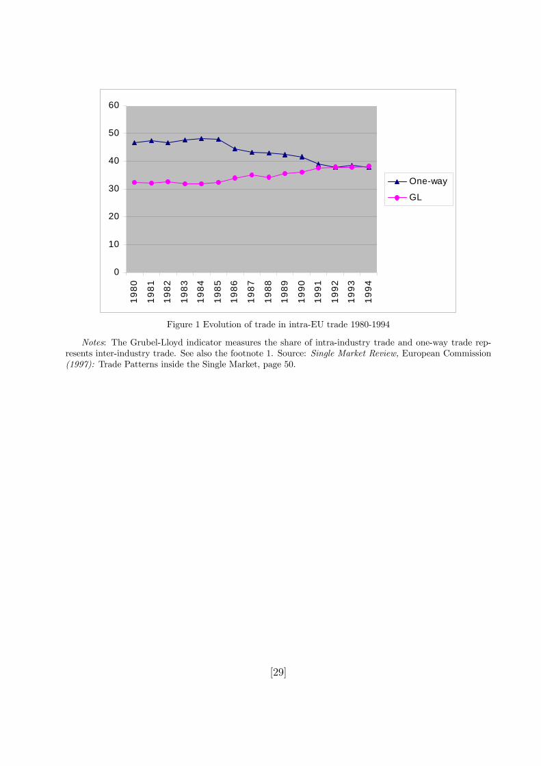
0

10

20

30

40

50

60

1980

1981

1982

1983

1984

1985

1986

1987

1988

1989

1990

1991

1992

1993

1994

One-way

GL

Figure 1 Evolution of trade in intra-EU trade 1980-1994

Notes: The Grubel-Lloyd indicator measures the share of intra-industry trade and one-way trade rep-resents inter-industry trade. See also the footnote 1. Source: Single Market Review, European Commission(1997): Trade Patterns inside the Single Market, page 50.

[29]

References

[1] Ahn SC, Lee YH, Schmidt P. 2001. GMM estimation of linear panel data models with time-varyingindividual effects. Journal of Econometrics 101: 219-255.

[2] Anderson PS. 1979. A theoretical foundation for the gravity equation. American Economic Review 69:106-116.

[3] Amemiya T, MaCurdy T. 1986. Instrumental variables estimation of an error components model. Econo-metrica 54: 869-880.

[4] Bai J, Ng S. 2002. Determine the number of factors in approximate factor models. Econometrica 70:191-221.

[5] Baldwin RE. 1994. Towards an integrated Europe. CEPR: London.

[6] Bergstrand JH. 1989. The generalized gravity equation, monopolistic competition, and factor propor-tions theory of international trade. Review of Economics and Statistics 71: 143-153.

[7] Bergstrand JH. 1990. The Heckscher-Olin-Samuelson model, the Linder hypothesis and the determinantsof bilateral intra-industry trade. Economic Journal 100: 1216-29.

[8] Bougheas S, Demetriades PO, Morgenroth ELW. 1999. Infrastructure, transport Costs and trade. Jour-nal of International Economics 47: 169-189.

[9] Brada JC, Mendez JA. 1988. Exchange rate risk, exchange rate regime and the volume of internationaltrade. Kylos 41: 263-80.

[10] Breusch T, Mizon G, Schmidt P. 1989. Efficient estimation using panel data. Econometrica 57: 695-700.

[11] Brun J, Carrere C, Guillaumont P, de Melo J. 2002. Has distance died? Evidence from a panel gravitymodel. Unpublished manuscript: University of d’Auvergne.

[12] Cheng I, Wall HJ. 2002. Controlling heterogeneity in gravity models of trade. Working Paper 1999-010C:Federal Reserve Bank of St. Louis.

[13] Davis DR. 2000. Understanding international trade patters: advantages of the 1990s. Unpublishedmanuscript: Columbia University.

[14] De Grauwe P, Skudelny F. 2000. The impact of EMU on trade flows. Weltwirtschaftliches Archiv 136:381-397.

[15] De Nardis S, Vicarelli C. 2003. The impact of the Euro on trade. ENEPRI Working Paper No. 17.

[16] De Sousa J, Disdier A. 2002. Trade, border effects and individual characteristics: A proper specification.Unpublished manuscript: University of Paris 1.

[17] de Souza LV. 2002. Trade effects of monetary integration in large, mature economies: a primer on theEuropean Monetary Union. Keil Working Paper No.1137.

[18] Deardorff, AV. 1984. Testing trade theories and predicting trade flows. Handbook of International Eco-nomics, Vol. 1.

[19] Deardorff AV. 1998. Determinants of bilateral trade: Does gravity work in a neoclassical world? NBER,Working Paper No.5377.

[20] Eaton J, Kortum S. 2002. Technology, geography, and trade. Econometrica 70: 1741-1779.

[21] Egger P. 2001. On the problem of endogenous unobserved effects of the gravity models. Working Paper:Austrian Institute of Economic Research, Vienna.

[22] Egger P. 2002. A note on the proper econometric specification of the gravity equation. Economics Letters66: 25-31.

[30]

[23] Egger P, Pfaffermayr M. 2002. The proper econometric specification of the gravity equation: A three-way model with bilateral interaction. Working Paper: Austrian Institute of Economic Research.

[24] Evenett SJ, Keller W. 2002. On the theories explaining the success of the gravity equation. Journal ofPolitical Economy 110: 281-316.

[25] Frenkel JA, Wei S. 1992. Trade blocs and currency blocs. NBER Working Paper No. 4335.

[26] Glink R, Rose AK. 2002. Does a currency union affect trade? The time series evidence. EuropeanEconomic Review 46: 1125-51.

[27] Grubel HG, Lloyd PJ. 1975. Intra-industry Trade, the Theory and Measurement of International Tradein Differentiated Products. MacMillan: London.

[28] Hausman JA. 1978. Specification tests in econometrics. Econometrica 46: 1251-1271.

[29] Hausman JA, Taylor WE. 1981. Panel data and unobservable individual effect. Econometrica 49: 1377-1398.

[30] Helpman E. 1987. Imperfect competition and international trade: Evidence from fourteen industrializedcountries. Journal of the Japanese and International Economies 1: 62-81.

[31] Hummels D, Levinsohn J. 1995. Monopolistic competition and international trade: Reconsidering theevidence. Quarterly Journal of Economics 110: 798-836.

[32] Jacquemin A, Sapir A. 1990. Competition and imports in the European Market, in European Integration:Trade and Industry. Cambridge University Press: Cambridge.

[33] Krugman PR. 1979. Increasing returns, monopolistic competition and international trade. Journal ofInternational Economics 9: 469-79.

[34] Leamer E. 1992. The interplay of the theory and data in the study of international trade, in Issues inContemporary Economics Vol. 2. New York University Press: New York.

[35] Linder SB. 1961. An Essay on Trade and Transformation. John Wiley and Son: New York.

[36] Markusen J, Wigle R. 1990. Expanding the volume of North-South trade. Economic Journal 100:1206-15.

[37] Martinez-Zaroso I, Nowak-Lehmann F. 2003. Augmented gravity model: An application to Mercosur-European Union trade flows. Journal of Applied Econometrics 18: 291-316.

[38] Matyas L. 1997. Proper econometric specification of the gravity model. The World Economy 20: 363-68.

[39] Matyas L, Konya L, Harris MN. 2002. Modelling export activity of eleven APEC countries. MelbourneInstitute Working Paper No. 5/00.

[40] Molle W. 1997. The Economics of European Integration: Theory, Practice and Policy. Ashgate Pub-lishing Limited.

[41] Pakko MR, Wall HJ. 2002. Reconsidering the effects of a currency union. Unpublished manuscript:Federal Reserve Bank of St. Louis

[42] Persson T. 2001. Currency union and trade: How large is the treatment effect? Economy Policy 33:435-448.

[43] Pesaran MH. 2002. Estimation and inference in large heterogeneous panels with cross section depen-dence. University of Cambridge DAE Working Paper No. 0305.

[44] Phillips PCB, Sul D. 2002. Dynamic panel estimation and homogeneity testing under cross sectiondependence. Cowles Foundation Discussion Paper No.1362: Yale University.

[45] Rose AK. 2002. The effect of common currency on international trade: Where do we stand? Unpublishedmanuscript, Haas School of Business, University of California, Berkeley.

[31]