gravitational acceleration and tidal e ects in spherical ... · gravitational acceleration and...
TRANSCRIPT

Applied Mathematical Sciences, Vol. 9, 2015, no. 123, 6107 - 6156HIKARI Ltd, www.m-hikari.com
http://dx.doi.org/10.12988/ams.2015.58536
Gravitational Acceleration and Tidal Effects
in Spherical-Symmetric Density Profiles
R. Caimmi
Physics and Astronomy Department, Padua UniversityVicolo Osservatorio 3/2, I-35122 Padova, Italy
Copyright c© 2015 R. Caimmi. This article is distributed under the Creative Commons
Attribution License, which permits unrestricted use, distribution, and reproduction in any
medium, provided the original work is properly cited.
Abstract
Pure power-law density profiles, ρ(r) ∝ rb−3, are classified in connectionwith the following reference cases: (i) isodensity, b = 3, ρ = const; (ii)isogravity, b = 2, g = const; (iii) isothermal, b = 1, v = [GM(r)/r]1/2 =const; (iv) isomass, b = 0, M = const. A restricted number of differ-ent families of density profiles including, in addition, cored power-law,generalized power-law, polytropes, are studied in detail with regard toboth one-component and two-component systems. Considerable effortis devoted to the existence of an extremum point (maximum absolutevalue) in the gravitational acceleration within the matter distribution.Predicted velocity curves are compared to the data inferred from ob-servations. Tidal effects on an inner subsystem are investigated andan application is made to globular clusters within the Galaxy. To thisaim, the tidal radius is defined by balancing the opposite gravitationalforces from the Galaxy and the selected cluster on a special point of thecluster boundary, lying between related centres of mass. The positionof 17 globular clusters with respect to the stability region, where thetidal radius exceeds the observed radius, is shown for assigned dark-to-visible mass ratios and density profiles, among those considered, whichare currently used for the description of galaxies and/or dark matterhaloes.
Keywords: cosmology: dark matter, galaxies: structure, globular clusters:general
6108 R. Caimmi
1 Introduction
Typical galaxies, such as spirals and giant ellipticals, are multi-component sys-tems mainly substructured as (1) nonbaryonic dark halo; (2) baryonic halo;(3) disk; (4) bulge; (5) inner accretion disk; (6) central accreting supermassiveblack hole, in brief hole. For sufficiently extended subsystems i.e. (1)-(4), adescription in terms of density profiles enables the determination of the theoret-ical circular velocity profile and the comparison with its empirical counterpartinferred from observations e.g., [25].
Strictly speaking, density profiles should relate to equilibrium equationse.g., [28], [26], [19], [39], but an acceptable fit to light distribution, via a mass-luminosity relation, could be sufficient for the description of related subsystemse.g., [21], [37], [29].
In most cases, each subsystem is treated separately and the model is asimple superposition of the various components. More self-consistent modelsshould account for the fact that each subsystem ought to readjust under thetidal action from the remaining subsystems. On the other hand, a simplesuperposition model may be adequate in deriving the general properties of amass distribution, provided the number of free parameters remains reasonablylow e.g., [15].
Though a quantitative (i.e. with regard to parameter values) classifica-tion of density profiles for one-component e.g., [42], [1], and two-componente.g., [17], [18], is long dating, still less effort has been devoted to a qualita-tive (i.e. with regard to intrinsic properties) classification. To this aim, thecurrent paper takes into consideration a restricted number of density profiles,part obeying an equilibrium equation and part being purely descriptive. Forsake of simplicity, attention shall be restricted to spherical-symmetric config-urations, even if the formulation maintains for homeoidally striated ellipsoidalconfigurations as far as radial properties are concerned e.g., [6], [8], [10]. Toemphasize the above mentioned property, spherical-symmetric density profilesshall be quoted henceforth as homeoidally striated spherical density profiles.
Pure power-law density profiles, ρ(r) ∝ rb−3, 0 ≤ b ≤ 3, are used to performa qualitative classification characterized by the following reference cases: (i)isodensity, b = 3, ρ = const; (ii) isogravity, b = 2, g = const; (iii) isothermal,b = 1, v = [GM(r)/r]1/2 = const; (iv) isomass, b = 0, M = const.
In the last case, ρ(r) = m0/r3, where m0 is a proportionality constant
dimensioned as a mass which, in addition, has to be infinitesimal of higherorder with respect to 1/ log r to avoid a logarithmic divergence in the mass,M(r). More specifically, m0 has to be infinitesimal of equal order with respectto r3 to ensure a finite nonzero mass at the centre, 0 < M(0) = M(r) < +∞.
A selected density profile can be classified as pseudo isodense, pseudo iso-gravity, pseudo isothermal, pseudo isomass, according if it is sufficiently close to

Gravitational acceleration and tidal effects in special density profiles 6109
the appropriate reference case. In particular, density profiles where 3 ≥ b > 2in the inner regions and 2 > b ≥ 0 in the outer regions, could exhibit anonmonotonic gravitational acceleration with the occurrence of an extremumpoint (maximum absolute value) inside the domain. Accordingly, further clas-sification of density profiles should include the presence or the absence of amaximum in |g| within a selected matter distribution.
Additional investigation, conceived as an application of the general theory,can be devoted to the stability of globular clusters against the tidal actionof the Galaxy via a simple formulation of tidal radius, involving balance ofopposite gravitational forces exerted from a selected cluster and the Galaxyon a special point on the cluster surface lying between related centres of masse.g., [41], [4]. For a fixed density profile, clusters where the tidal radius exceedsthe observed radius are considered bound, if otherwise (partially) unbound.
The position of globular clusters can be plotted together with the stabilityregion, and the number of bound and (partially) unbound globular clusterscan be determined for selected Galactic density profiles. Finally, Galacticdensity profiles can be constrained according if globular clusters showing nosign of tidal tails or tidal streams lie within the instability region and viceversa. Though a more accurate definition of tidal radius should be used toinfer quantitative conclusions, still the trend is expected to be similar and thevalidity of the method is left unchanged.
The current paper is structured in the following way. One-component,homeoidally striated spherical density profiles are described in Section 2, wherefurther attention is devoted to a few families of density profiles, namely (a)pure power-law; (b) cored power-law; (c) polytropes; (d) Plummer [34]; (e)Hernquist [26]; (f) Begeman et al. [2]; (g) Spano et al. [38]; (h) Burkert [5].Two-component, concentric, homeoidally striated spherical density profiles aredescribed in Section 3, where further attention is devoted to a few combinationsof density profiles, namely (i) Plummer-Begeman et al.; (j) Hernquist-Begemanet al; (k) Plummer-Spano et al.; (l) Hernquist-Spano et al. Tidal effects onembedded sybsystems are analysed in Section 4, where the tidal radius is de-fined via gravitational balance on a special point and an application to globularclusters within galaxies is performed, with regard to density profiles currentlyused for the description of galaxies and/or dark matter haloes, among thoseconsidered. The results are discussed in Section 5, where the particularizationto a sample of Galactic globular clusters is also shown. Finally, the conclusionis drawn in Section 6. Further details on specific arguments are shown in theAppendix.
6110 R. Caimmi
2 Homeoidally striated spherical density pro-
files
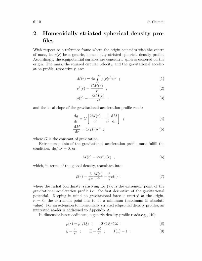
With respect to a reference frame where the origin coincides with the centreof mass, let ρ(r) be a generic, homeoidally striated spherical density profile.Accordingly, the equipotential surfaces are concentric spheres centered on theorigin. The mass, the squared circular velocity, and the gravitational acceler-ation profile, respectively, are:
M(r) = 4π∫ r
0ρ(r)r2 dr ; (1)
v2(r) =GM(r)
r; (2)
g(r) = −GM(r)
r2; (3)
and the local slope of the gravitational acceleration profile reads:
dg
dr= G
[2M(r)
r3− 1
r2
dM
dr
]; (4)
dM
dr= 4πρ(r)r2 ; (5)
where G is the constant of gravitation.Extremum points of the gravitational acceleration profile must fulfill the
condition, dg/ dr = 0, or:
M(r) = 2πr3ρ(r) ; (6)
which, in terms of the global density, translates into:
ρ(r) =3
4π
M(r)
r3=
3
2ρ(r) ; (7)
where the radial coordinate, satisfying Eq. (7), is the extremum point of thegravitational acceleration profile i.e. the first derivative of the gravitationalpotential. Keeping in mind no gravitational force is exerted at the origin,r = 0, the extremum point has to be a minimum (maximum in absolutevalue). For an extension to homeoidally striated ellipsoidal density profiles, aninterested reader is addressed to Appendix A.
In dimensionless coordinates, a generic density profile reads e.g., [10]:
ρ(r) = ρ†f(ξ) ; 0 ≤ ξ ≤ Ξ ; (8)
ξ =r
r†; Ξ =
R
r†; f(1) = 1 ; (9)
Gravitational acceleration and tidal effects in special density profiles 6111
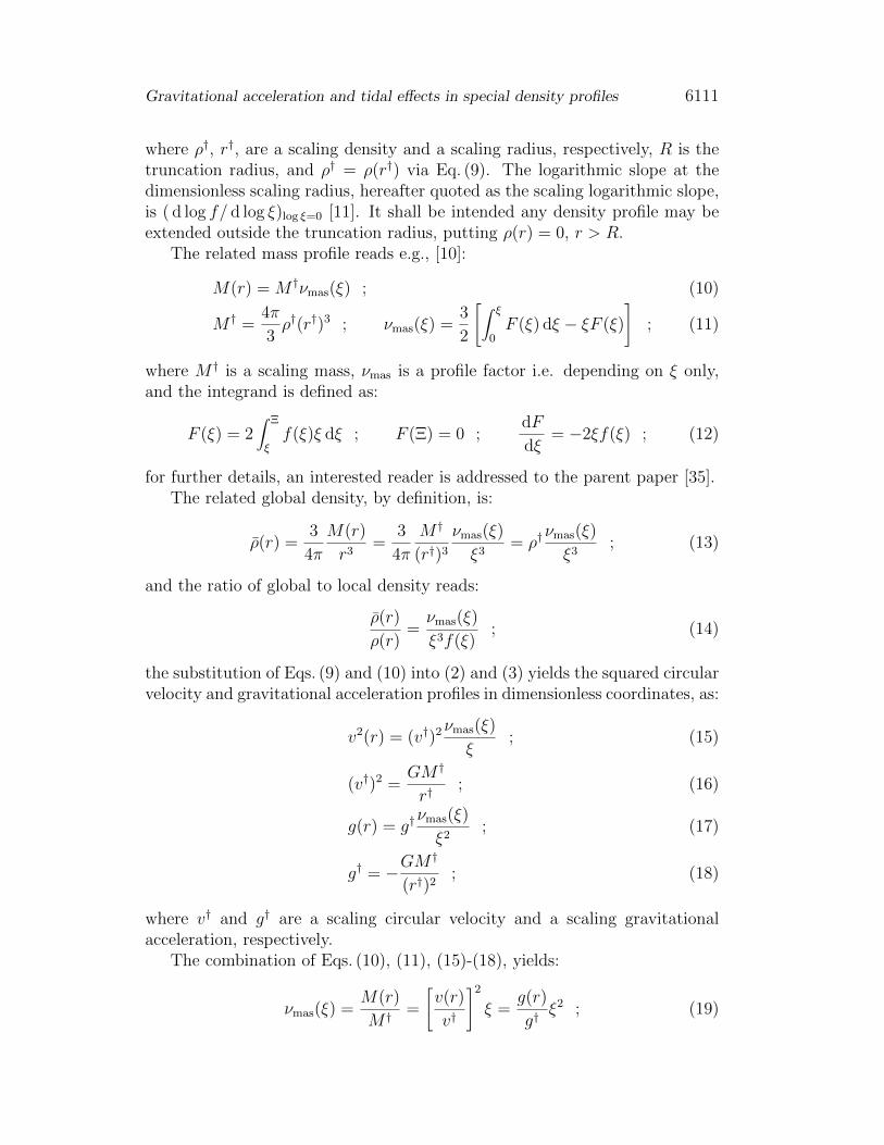
where ρ†, r†, are a scaling density and a scaling radius, respectively, R is thetruncation radius, and ρ† = ρ(r†) via Eq. (9). The logarithmic slope at thedimensionless scaling radius, hereafter quoted as the scaling logarithmic slope,is ( d log f/ d log ξ)log ξ=0 [11]. It shall be intended any density profile may beextended outside the truncation radius, putting ρ(r) = 0, r > R.
The related mass profile reads e.g., [10]:
M(r) = M †νmas(ξ) ; (10)
M † =4π
3ρ†(r†)3 ; νmas(ξ) =
3
2
[∫ ξ
0F (ξ) dξ − ξF (ξ)
]; (11)
where M † is a scaling mass, νmas is a profile factor i.e. depending on ξ only,and the integrand is defined as:
F (ξ) = 2∫ Ξ
ξf(ξ)ξ dξ ; F (Ξ) = 0 ;
dF
dξ= −2ξf(ξ) ; (12)
for further details, an interested reader is addressed to the parent paper [35].The related global density, by definition, is:
ρ(r) =3
4π
M(r)
r3=
3
4π
M †
(r†)3
νmas(ξ)
ξ3= ρ†
νmas(ξ)
ξ3; (13)
and the ratio of global to local density reads:
ρ(r)
ρ(r)=νmas(ξ)
ξ3f(ξ); (14)
the substitution of Eqs. (9) and (10) into (2) and (3) yields the squared circularvelocity and gravitational acceleration profiles in dimensionless coordinates, as:
v2(r) = (v†)2νmas(ξ)
ξ; (15)
(v†)2 =GM †
r†; (16)
g(r) = g†νmas(ξ)
ξ2; (17)
g† = −GM†
(r†)2; (18)
where v† and g† are a scaling circular velocity and a scaling gravitationalacceleration, respectively.
The combination of Eqs. (10), (11), (15)-(18), yields:
νmas(ξ) =M(r)
M † =
[v(r)
v†
]2
ξ =g(r)
g†ξ2 ; (19)

6112 R. Caimmi
and the combination of Eqs. (7) and (14) yields:
νmas(ξ)
ξ3f(ξ)=
3
2; (20)
the solution of which is the extremum point of the gravitational accelerationprofile in dimensionless coordinates.
Let the isodensity surface where the gravitational acceleration attains theextremum point be defined as effective surface of the system, and the relatedradius as effective radius. In absence of an extremum point, the effectiveradius necessarily takes place on the boundary of the domain, either reff = 0or reff = R, in dimensionless coordinates either ξeff = 0 or ξeff = Ξ.
The particularization of the above results to some special families of densityprofiles shall be performed in the following subsections.
2.1 Pure power-law density profiles
Pure power-law density profiles are defined as e.g., [9]:
f(ξ) = ξb−3 ; 0 ≤ ξ ≤ Ξ ; 0 ≤ b ≤ 3 ; (21)
where b > 3 implies increasing density for increasing radial coordinate, andb < 0 implies infinite central mass. The scaling logarithmic slope is:(
d log f
d log ξ
)log ξ=0
= b− 3 ; (22)
which is constant in the case under consideration.The substitution of Eq. (21) into (10)-(18) yields after some algebra:
F (ξ) =2
b− 1(Ξb−1 − ξb−1) ; (23)
νmas(ξ) =3
bξb ; (24)
ρ(r)
ρ†=
3
bξb−3 ; (25)
ρ(r)
ρ(r)=
3
b; (26)
v2(r)
(v†)2=
3
bξb−1 ; (27)
g
g†=
3
bξb−2 ; (28)
where b = 3 corresponds to the isodensity (ρ = const) sphere, b = 2 to theisogravity (g = const) sphere, b = 1 to the isothermal (v2 = GM(r)/r = const)
Gravitational acceleration and tidal effects in special density profiles 6113
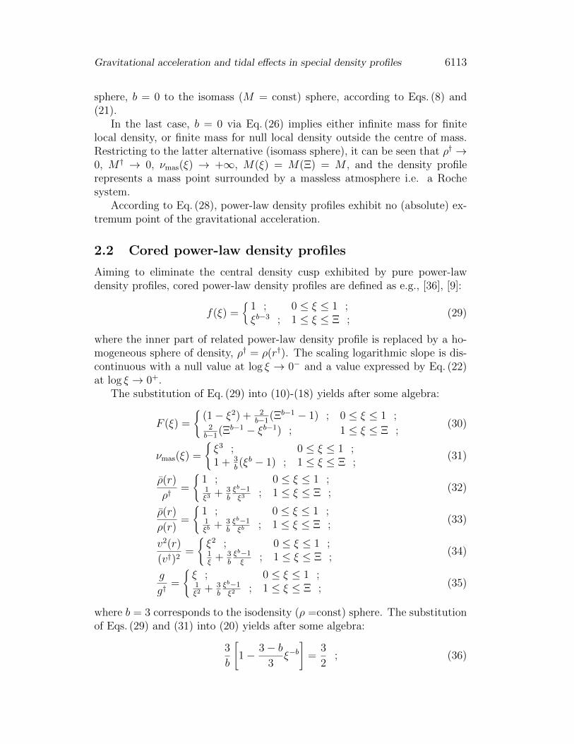
sphere, b = 0 to the isomass (M = const) sphere, according to Eqs. (8) and(21).
In the last case, b = 0 via Eq. (26) implies either infinite mass for finitelocal density, or finite mass for null local density outside the centre of mass.Restricting to the latter alternative (isomass sphere), it can be seen that ρ† →0, M † → 0, νmas(ξ) → +∞, M(ξ) = M(Ξ) = M , and the density profilerepresents a mass point surrounded by a massless atmosphere i.e. a Rochesystem.
According to Eq. (28), power-law density profiles exhibit no (absolute) ex-tremum point of the gravitational acceleration.
2.2 Cored power-law density profiles
Aiming to eliminate the central density cusp exhibited by pure power-lawdensity profiles, cored power-law density profiles are defined as e.g., [36], [9]:
f(ξ) ={
1 ; 0 ≤ ξ ≤ 1 ;ξb−3 ; 1 ≤ ξ ≤ Ξ ;
(29)
where the inner part of related power-law density profile is replaced by a ho-mogeneous sphere of density, ρ† = ρ(r†). The scaling logarithmic slope is dis-continuous with a null value at log ξ → 0− and a value expressed by Eq. (22)at log ξ → 0+.
The substitution of Eq. (29) into (10)-(18) yields after some algebra:
F (ξ) =
{(1− ξ2) + 2
b−1(Ξb−1 − 1) ; 0 ≤ ξ ≤ 1 ;
2b−1
(Ξb−1 − ξb−1) ; 1 ≤ ξ ≤ Ξ ;(30)
νmas(ξ) =
{ξ3 ; 0 ≤ ξ ≤ 1 ;1 + 3
b(ξb − 1) ; 1 ≤ ξ ≤ Ξ ;
(31)
ρ(r)
ρ†=
{1 ; 0 ≤ ξ ≤ 1 ;1ξ3
+ 3bξb−1ξ3
; 1 ≤ ξ ≤ Ξ ; (32)
ρ(r)
ρ(r)=
{1 ; 0 ≤ ξ ≤ 1 ;1ξb
+ 3bξb−1ξb
; 1 ≤ ξ ≤ Ξ ; (33)
v2(r)
(v†)2=
{ξ2 ; 0 ≤ ξ ≤ 1 ;1ξ
+ 3bξb−1ξ
; 1 ≤ ξ ≤ Ξ ;(34)
g
g†=
{ξ ; 0 ≤ ξ ≤ 1 ;1ξ2
+ 3bξb−1ξ2
; 1 ≤ ξ ≤ Ξ ; (35)
where b = 3 corresponds to the isodensity (ρ =const) sphere. The substitutionof Eqs. (29) and (31) into (20) yields after some algebra:
3
b
[1− 3− b
3ξ−b
]=
3
2; (36)
6114 R. Caimmi
and the extremum point of the gravitational acceleration is defined by thesolution of Eq. (36) as:
ξ =
(2
3
3− b2− b
)1/b
; (37)
where ξ ≥ 1 in that no extremum point exists for the inner homogeneoussphere, 0 ≤ ξ ≤ 1, according to Eq. (28), and, on the other hand, ξ ≤ Ξ,according to Eq. (29), which implies the following:
1 ≤ φ(b) =
(2
3
3− b2− b
)1/b
≤ Ξ ; (38)
limb→0
(2
3
3− b2− b
)1/b
= exp(
1
6
); (39)
where φ(b) is defined within the domain, 0 ≤ b < 2, b = 3, as powers with realexponents must necessarily exhibit nonnegative basis, and is monotonicallyincreasing.
In conclusion, an extremum point is attained by the gravitational accel-eration for sufficiently steep (0 ≤ b < 2) cored power-law density profiles,provided Eq. (38) is satisfied. In particular, Ξ ≥ exp(1/6) for b = 0 i.e. ageneralized Roche system.
2.3 Polytropic density profiles
Polytropic spheres obey the Lane-Emden equation e.g., [16] (Chap. IV):
1
ξ2LE
d
dξLE
(ξ2
LE
dθ
dξLE
)= −θn ; (40)
θ(0) = 1 ; θ(ΞLE) = 0 ;
(dθ
dξLE
)0
= 0 ; (41)
θ(ξLE) = 1− 1
6ξ2
LE +n
120ξ4
LE − ... ; 0 ≤ ξLE < 1 ; (42)
where n is the polytropic index and the dimensionless radial coordinate, ξLE,and the dimensionless density, θn, are related to their dimensional counterpartsas:
r = αLEξLE ; R = αLEΞLE ; αLE =
(n+ 1)Kλ1+1/nLE
4πGλ2LE
1/2
; (43)
ρ(r) = λLEθn(ξLE) ; ρ(0) = λLE ; ρ(R) = 0 ; (44)
where λLE is the central density, Kλ1+1/nLE the central pressure, and αLE the
polytropic scaling radius. Polytropic density profiles lie between the limiting
Gravitational acceleration and tidal effects in special density profiles 6115
cases of homogeneous configurations (n = 0) and Roche systems or Plummersystems (n = 5).
The relations between current and polytropic dimensionless density andradial coordinate, may be deduced by comparison of Eqs. (8) and (9) with (44)and (43), respectively. The result is:
f(ξ) =λLE
ρ†θn(ξLE) ; (45)
ξ =αLE
r†ξLE ; Ξ =
αLE
r†ΞLE ; (46)
and the boundary condition, f(1) = 1, translates into:
θ
(r†
αLE
)=
(ρ†
λLE
)1/n
; (47)
where, in particular:
limn→0
(ρ†
λLE
)1/n
= 1− 1
6
(r†
αLE
)2
; (48)
for homogeneous configurations, using next Eq. (60).As the Lane-Emden equation, Eq. (40), and related solutions, have widely
been studied in literature e.g., [16] (Chap. IV), [27], the quantities of interestfor polytropic density profiles shall be expressed in terms of the dimensionlessdensity, θn, and the dimensionless radial coordinate, ξLE.
Accordingly, the scaling logarithmic slope is:(d log f
d log ξ
)log ξ=0
= n
(d log θ
d log ξLE
d log ξLE
d log ξ
)log ξ=0
= n
(d log θ
d log ξLE
)log ξLE=log(r†/αLE)
; (49)
and Eqs. (10), (11), (13), (14), (15), (17) and (20), take the equivalent forme.g., [16] (Chap. IV, §6):
M(r) = −MLEξ2LE
dθ
ξLE
; (50)
MLE = 4πα3LEλLE ; (51)
ρ(r)
λLE
= − 3
ξLE
dθ
dξLE
; (52)
ρ(r)
ρ(r)= − 3
ξLE
dθ/ dξLE
θn(ξLE); (53)
6116 R. Caimmi
[v(r)
vLE
]2
=GM(r)
v2LEr
= −ξLEdθ
dξLE
; (54)
v2LE =
GMLE
αLE
; (55)
g(r)
gLE
= −GM(r)
gLE r2= − dθ
dξLE
; (56)
gLE = −GMLE
α2LE
; (57)
1
ξLE
dθ
dξLE
= −1
2θn(ξLE) ; (58)
where the last result follows from Eq. (41), implying the existence of a solutionto Eq. (58) for n > 0, as θ is continuous together with its first and secondderivates via Eq. (40).
The substitution of Eq. (40) into (58) yields after some algebra:
d2θ
dξ2LE
= 0 ; (59)
which shows that, for polytropic density profiles, the extremum point of thegravitational acceleration coincides with the extremum point of the first deriva-tive of θ, as expected, the gravitational potential inside polytropic spheresbeing proportional to θ e.g., [16] (Chap. IV, §7).
In the special cases, n = 0, 1, 5, Eq. (40) can analytically be integrated.The result is e.g., [16] (Chap. IV, §4):
θ(ξLE) = 1− 1
6ξ2
LE ; ΞLE =√
6 ; n = 0 ; (60)
θ(ξLE) =sin ξLE
ξLE
; ΞLE = π ; n = 1 ; (61)
θ(ξLE) =(
1 +1
3ξ2
LE
)−1/2
; ΞLE → +∞ ; n = 5 ; (62)
accordingly, Eq. (58) has no solution for n = 0, as expected for homogeneousconfigurations, and:
ξLE cos ξLE − sin ξLE
ξ2LE
= −1
2sin ξLE ; (63)
for n = 1, which has a solution, ξLE ≈ 2.081 575 99, and:
−1
2
(1 +
1
3ξ2
LE
)−3/2 2
3ξLE = −1
2ξLE
(1 +
1
3ξ2
LE
)−5/2
; (64)
for n = 5, which has a solution, ξLE =√
3/2 ≈ 1.224 744 871.

Gravitational acceleration and tidal effects in special density profiles 6117
In conclusion, an extremum point is exhibited by the gravitational accel-eration for inhomogeneous polytropic density profiles (0 < nmin ≤ n ≤ 5),where the solution of related transcendental equation can readily be deter-mined in the special cases, n = 1, 5, via Eqs. (63), (64), respectively. Thethreshold, nmin, 0 < nmin < 1, is defined by equating the solution of Eq. (58)to the dimensionless radius, ξLE(nmin) = ΞLE(nmin), as n < nmin would implyξLE(nmin) > ΞLE(nmin), which lies outside the domain, 0 ≤ ξLE ≤ ΞLE.
2.4 Plummer density profiles
Plummer density profiles [34], hereafter quoted as P density profiles, are noth-ing but n = 5 polytropes represented by Eqs. (8), (9), via (45)-(47), whereparameters are interrelated as [14]:
ξ =ξLE√
3; r† =
√3αLE ; ρ† =
λLE
25/2; (65)
the result is [14]:
f(ξ) =25/2
(1 + ξ2)5/2; (66)
where the scaling logarithmic slope reads:(d log f
d log ξ
)log ξ=0
= −5
2; (67)
and the substitution of Eq. (66) into (10)-(18) yields after some algebra:
F (ξ) =27/2
3
[1
(1 + ξ2)3/2− 1
(1 + Ξ2)3/2
]; (68)
νmas(ξ) =25/2ξ3
(1 + ξ2)3/2; (69)
ρ(r)
ρ†=
25/2
(1 + ξ2)3/2; (70)
ρ(r)
ρ(r)= 1 + ξ2 ; (71)[
v(r)
v†
]2
=25/2ξ2
(1 + ξ2)3/2; (72)
g(r)
g†=
25/2ξ
(1 + ξ2)3/2; (73)
finally, the particularization of Eq. (20) to the case under consideration reads:
1 + ξ2 =3
2; (74)

6118 R. Caimmi
which shows an extremum point of the gravitational acceleration at ξ =1/√
2 ≈ 0.707 106 781, in agreement with Eqs. (64) and (65).
2.5 Hernquist density profiles
Hernquist density profiles [26], hereafter quoted as H density profiles, are de-fined as e.g., [14]:
f(ξ) =8
ξ(1 + ξ)3; (75)
where the scaling logarithmic slope reads:(d log f
d log ξ
)log ξ=0
= −5
2; (76)
and the substitution of Eq. (75) into (10)-(18) yields after some algebra:
F (ξ) = 8
[1
(1 + ξ)2− 1
(1 + Ξ)2
]; (77)
νmas(ξ) =12ξ2
(1 + ξ)2; (78)
ρ(r)
ρ†=
12
ξ(1 + ξ)2; (79)
ρ(r)
ρ(r)=
3
2(1 + ξ) ; (80)[
v(r)
v†
]2
=12ξ
(1 + ξ)2; (81)
g(r)
g†=
12
(1 + ξ)2; (82)
finally, the particularization of Eq. (20) to the case under consideration reads:
3
2(1 + ξ) =
3
2; (83)
which implies no extremum point for the gravitational acceleration inside thedomain. In addition, Eq. (82) discloses that a finite gravitational accelerationoccurs even if a test particle lies infinitely close to the centre.
2.6 Generalized power-law density profiles
Generalized power-law density profiles are defined as e.g., [3]:
f(ξ) =Cγ + 1
Cγ + ξγ(Cα + 1)χ
(Cα + ξα)χ; (84)
where the following families are worth of note.
Gravitational acceleration and tidal effects in special density profiles 6119
• Cγ = 0; Cα = 0; generalized power-law density profiles reduce to purepower-law density profiles with exponent, β, expressed as:
β = γ + αχ ; χ =β − γα
; (85)
which shows the meaning of the exponent, χ, appearing in Eq. (84).
• Cγ = 0; Cα = 1; generalized power-law density profiles reduce to a subclassanalysed in earlier attempts [26], [42], hereafter quoted as Z density pro-files. Special cases are P density profiles, (α, χ, γ) = (2, 5/2, 0); H densityprofiles, (α, χ, γ) = (1, 3, 1); pseudo isothermal density profiles e.g., [2],(α, χ, γ) = (2, 1, 0), hereafter quoted as I density profiles; generalizedpseudo isothermal density profiles [38], (α, χ, γ) = (2, 3/2, 0), hereafterquoted as S density profiles.
• Cγ = 1; Cα = 0; generalized power-law density profiles reduce to a subclassof Z density profiles, (α, χ, γ) = (γ, 1, αχ), including I density profiles.
• Cγ = 1; Cα = 1; generalized power-law density profiles reduce to a subclassof density profiles including a special case analysed in an earlier attempt[5], (α, χ, γ) = (2, 1, 1), hereafter quoted as B density profiles.
For generalized power-law density profiles, the scaling logarithmic slopereads: (
d log f
d log ξ
)log ξ=0
= − γ
Cγ + 1− β − γCα + 1
; (86)
which, for Z density profiles, reduces to:(d log f
d log ξ
)log ξ=0
= −β + γ
2; (87)
the geometrical meaning of the dimensionless scaling radius is analysed inAppendix B.
The substitution of Eq. (84) into (10)-(18) yields, in general, integrals whichcannot be analytically calculated. For this reason, further considerations shallbe restricted to the above mentioned special cases, where the primitive func-tions can be explicitly expressed.
2.7 Pseudo isothermal density profiles
For I density profiles, Eq. (84) reduces to:
f(ξ) =2
1 + ξ2; (88)

6120 R. Caimmi
where the scaling logarithmic slope reads:(d log f
d log ξ
)log ξ=0
= −1 ; (89)
according to Eq. (87).
The substitution of Eq. (88) into (10)-(18) yields after some algebra:
F (ξ) = 2 ln1 + Ξ2
1 + ξ2; (90)
νmas(ξ) = 6(ξ − arctan ξ) ; (91)
ρ(r)
ρ†=
6
ξ3(ξ − arctan ξ) ; (92)
ρ(r)
ρ(r)=
3
ξ3(1 + ξ2)(ξ − arctan ξ) ; (93)[
v(r)
v†
]2
=6
ξ(ξ − arctan ξ) ; (94)
g(r)
g†=
6
ξ2(ξ − arctan ξ) ; (95)
finally, the particularization of Eq. (20) to the case under consideration reads:
arctan ξ =ξ(2 + ξ2)
2(1 + ξ2); (96)
and the extremum point for the gravitational acceleration is defined by thesolution of Eq. (96), as ξ ≈ 1.514 994 606.
2.8 Spano et al. density profiles
For S density profiles, Eq. (84) reduces to:
f(ξ) =23/2
(1 + ξ2)3/2; (97)
where the scaling logarithmic slope reads:(d log f
d log ξ
)log ξ=0
= −3
2; (98)
according to Eq. (87).

Gravitational acceleration and tidal effects in special density profiles 6121
The substitution of Eq. (97) into (10)-(18) yields after some algebra:
F (ξ) = 25/2
(1√
1 + ξ2− 1√
1 + Ξ2
); (99)
νmas(ξ) = 6√
2
(arcsinh ξ − ξ√
1 + ξ2
); (100)
ρ(r)
ρ†=
6√
2
ξ3
(arcsinh ξ − ξ√
1 + ξ2
); (101)
ρ(r)
ρ(r)=
3√
2
ξ3(1 + ξ2)3/2
(arcsinh ξ − ξ√
1 + ξ2
); (102)[
v(r)
v†
]2
=6√
2
ξ
(arcsinh ξ − ξ√
1 + ξ2
); (103)
g(r)
g†=
6√
2
ξ2
(arcsinh ξ − ξ√
1 + ξ2
); (104)
finally, the particularization of Eq. (20) to the case under consideration reads:
arcsinh ξ =ξ(2 + 3ξ2)
2(1 + ξ2)3/2; (105)
and the extremum point for the gravitational acceleration is defined by thesolution of Eq. (105), as ξ ≈ 1.027 115 657.
2.9 Burkert density profiles
For B density profiles, Eq. (84) reduces to:
f(ξ) =2
1 + ξ
2
1 + ξ2; (106)
where the scaling logarithmic slope reads:(d log f
d log ξ
)log ξ=0
= −3
2; (107)
according to Eq. (87).The substitution of Eq. (106) into (10)-(18) yields after some algebra:
F (ξ) = −2 ln1 + ξ2
1 + Ξ2+ 4 ln
1 + ξ
1 + Ξ+ 4(arctan Ξ− arctan ξ) ; (108)
νmas(ξ) = 3[ln(1 + ξ2) + 2 ln(1 + ξ)− 2 arctan ξ] ; (109)
ρ(r)
ρ†=
3
ξ3[ln(1 + ξ2) + 2 ln(1 + ξ)− 2 arctan ξ] ; (110)

6122 R. Caimmi
ρ(r)
ρ(r)=
3
4
1
ξ3[ln(1 + ξ2) + 2 ln(1 + ξ)− 2 arctan ξ] ; (111)[
v(r)
v†
]2
=3
ξ[ln(1 + ξ2) + 2 ln(1 + ξ)− 2 arctan ξ] ; (112)
g(r)
g†=
3
ξ2[ln(1 + ξ2) + 2 ln(1 + ξ)− 2 arctan ξ] ; (113)
finally, the particularization of Eq. (20) to the case under consideration reads:
ln(1 + ξ2) + 2 ln(1 + ξ)− 2 arctan ξ =2ξ3
(1 + ξ)(1 + ξ2); (114)
and the extremum point for the gravitational acceleration is defined by thesolution of Eq. (114), as ξ ≈ 0.963 398 283.
2.10 Gravitational acceleration vs. density profile
The dependence of the gravitational acceleration on the density profile can berelated to the dimensionless effective radius, ξeff , where the maximum absolutevalue is attained. For the density profiles considered in the current Section,the results are listed in Table 1 together with values of related parameters.An inspection of Table 1 shows the occurrence of an extremum point (max-imum absolute value) in the gravitational acceleration distribution, with theexception of pure power-law, cored power-law (2 ≤ b ≤ 3), H density profiles,and the possible exception of cored power-law (0 ≤ b < 2) density profiles,according to the selected dimensionless truncation radius, Ξ.
3 Two-component density profiles
Let ρi(r), ρj(r), be generic but concentric homeoidally striated spherical den-sity profiles, and Mi(r), Mj(r), related masses enclosed within the distance, r,from the centre. The total mass, the squared circular velocity, and the gravi-tational acceleration are expressed by Eqs. (1)-(3) where ρ(r) = ρi(r) + ρj(r),M(r) = Mi(r) +Mj(r), which implies ρ(r) = ρi(r) + ρj(r).
It can be seen the validity of Eq. (7) for each subsystem i.e. the existenceof an extremum point of related gravitational acceleration, gu = −GMu(r)/r
2,u = i, j, is a necessary condition for the validity of Eq. (7) for the whole systemi.e. the existence of an extremum point of related gravitational acceleration,g = gi + gj.
In dimensionless coordinates, generic density profiles are expressed by Eqs. (8)-(20), provided each quantity is indexed by i or j, according to the selected

Gravitational acceleration and tidal effects in special density profiles 6123
Table 1: Parameters of one-component density profiles considered in the text:polytropic index, n, for polytropes; constants, Cγ, Cα, and exponents, α, χ, γ,β, for generalized power-law density profiles, Eqs. (84)-(85); and dimensionlesseffective radius, ξeff . An extremum point for the gravitational accelerationoccurs only if 0 < ξeff < Ξ. For polytropic density profiles, ξeff = Ξ, n = 0, and
ξeff =√
3/2, n = 5, respectively. For Plummer density profile, ξeff = 1/√
2.
The notations specifying power-law density profiles, (0-2) and (2-3), are to beintended as (0 ≤ b ≤ 2) and (2 ≤ b ≤ 3), respectively. See text for furtherdetails.
density profile n Cγ Cα α χ γ β ξeff
pure power-law (0-2) 0 0 α β−γα
γ β 0
pure power-law (2-3) 0 0 α β−γα
γ β Ξ
cored power-law (0-2) min[(
23
3−b2−b
)1/b,Ξ]
cored power-law (2-3) Ξpolytropic 0 2.449 489 743polytropic 1 2.081 575 99polytropic 5 1.224 744 871Plummer [34] 0 1 2 2.5 0 5 0.707 106 781Hernquist [26] 0 1 1 3.0 1 4 0Begeman et al. [2] 0 1 2 1.0 0 2 1.514 994 606Spano et al. [38] 0 1 2 1.5 0 3 1.027 115 657Burkert [5] 1 1 2 1.0 1 3 0.963 398 283
6124 R. Caimmi
subsystem. In addition, the following relations hold e.g., [14]:
ξi = y†ξj ;Ξj
Ξi
=y
y†;
νj,mas(r)
νi,mas(r)=m(r)
m†; (115a)
y =Rj
Ri
; y† =r†j
r†i; m(r) =
Mj(r)
Mi(r); m† =
M †j
M †i
; (115b)
ρ†j
ρ†i=
m†
(y†)3; (115c)
where y ≥ 1 without loss of generality, which implies i is the inner subsystemand j the outer unless their surfaces coincide.
Using Eqs. (10)-(18) and (115), the mass enclosed within the radius, r, andrelated squared circular velocity and gravitational acceleration are expressedas:
M(r) = M †i νi,mas(ξi) +M †
j νj,mas(ξj) ; (116)
v2(r) = (v†i )2νi,mas(ξi)
ξi+ (v†j)
2νj,mas(ξj)
ξj; (117)
g(r) = g†iνi,mas(ξi)
ξ2i
+ g†jνj,mas(ξj)
ξ2j
; (118)
and the extremum point of the gravitational acceleration, via Eqs. (7)-(20) and(115), is the solution of the following equation:
ρ†i
[νi,mas(ξi)
ξ3i
− 3
2fi(ξi)
]+ ρ†j
[νj,mas(ξj)
ξ3j
− 3
2fj(ξj)
]= 0 ; (119)
where ξi and ξj are related via Eqs. (115a)-(115b).Some special density distributions shall be considered in the following, and
Eq. (119) shall be written in terms of the additional parameters, m† and y†,from which the extremum points of the gravitational acceleration also depend.
3.1 PI density profiles
In the special case of an inner P density profile, i =P, and an outer I densityprofile, j =I, the substitution of Eqs. (66)-(73) and (88)-(95) into (115)-(118)yields:
ξP = y†ξI ; (120)
m(r) = m†6(ξI − arctan ξI)
25/2ξ3P(1 + ξ2
P)−3/2; (121)
M(r) = M †P
25/2ξ3P
(1 + ξ2P)3/2
+M †I 6(ξI − arctan ξI) ; (122)

Gravitational acceleration and tidal effects in special density profiles 6125
v2(r) = (v†P)2 25/2ξ2P
(1 + ξ2P)3/2
+ (v†I )2 6(ξI − arctan ξI)
ξI
; (123)
g(r) = g†P25/2ξP
(1 + ξ2P)3/2
+ g†I6(ξI − arctan ξI)
ξ2I
; (124)
and the extremum point of the gravitational acceleration is the solution ofEq. (119) particularized to the case under consideration, which after some al-gebra reads:
23/2ρ†P(1 + ξ2
P)3/2
2ξ2P − 1
1 + ξ2P
+ 3ρ†I
[2 + ξ2
I
ξ2I (1 + ξ2
I )− 2 arctan ξI
ξ3I
]= 0 ; (125)
that shows an additional dependence on the parameters, m†, y†, via Eqs. (115c)and (120), respectively.
3.2 HI density profiles
In the special case of an inner H density profile, i =H, and an outer I densityprofile, j =I, the substitution of Eqs. (75)-(82) and (88)-(95) into (115)-(118)yields:
ξH = y†ξI ; (126)
m(r) = m†ξI − arctan ξI
2ξ2H(1 + ξH)−2
; (127)
M(r) = M †H
12ξ2H
(1 + ξH)2+M †
I 6(ξI − arctan ξI) ; (128)
v2(r) = (v†H)2 12ξH
(1 + ξH)2+ (v†I )2 6(ξI − arctan ξI)
ξI
; (129)
g(r) = g†H12
(1 + ξH)2+ g†I
6(ξI − arctan ξI)
ξ2I
; (130)
and the extremum point of the gravitational acceleration is the solution ofEq. (119) particularized to the case under consideration, which after some al-gebra reads:
12ρ†H(1 + ξH)3
+ 3ρ†I
[2 + ξ2
I
ξ2I (1 + ξ2
I )− 2 arctan ξI
ξ3I
]= 0 ; (131)
that shows an additional dependence on the parameters, m†, y†, via Eqs. (115c)and (126), respectively.
6126 R. Caimmi
3.3 PS density profiles
In the special case of an inner P density profile, i =P, and an outer S densityprofile, j =S, the substitution of Eqs. (66)-(73) and (97)-(104) into (115)-(118)yields:
ξP = y†ξS ; (132)
m(r) = m†6√
2[arcsinh ξS − ξS(1 + ξ2S)−1/2]
25/2ξ3P(1 + ξ2
P)−3/2; (133)
M(r) = M †P
25/2ξ3P
(1 + ξ2P)3/2
+M †S6√
2
arcsinh ξS −ξS√
1 + ξ2S
; (134)
v2(r) = (v†P)2 25/2ξ2P
(1 + ξ2P)3/2
+ (v†S)26√
2
arcsinh ξS
ξS
− 1√1 + ξ2
S
; (135)
g(r) = g†P25/2ξP
(1 + ξ2P)3/2
+ g†S6√
2
ξS
arcsinh ξS
ξS
− 1√1 + ξ2
S
; (136)
and the extremum point of the gravitational acceleration is the solution ofEq. (119) particularized to the case under consideration, which after some al-gebra reads:
23/2ρ†P(1 + ξ2
P)3/2
2ξ2P − 1
1 + ξ2P
+3√
2ρ†Sξ2
S
[2
arcsinh ξS
ξS
− 2 + 3ξ2S
(1 + ξ2S)3/2
]= 0 ; (137)
that shows an additional dependence on the parameters, m†, y†, via Eqs. (115c)and (132), respectively.
3.4 HS density profiles
In the special case of an inner H density profile, i =H, and an outer S densityprofile, j =S, the substitution of Eqs. (75)-(82) and (97)-(104) into (115)-(118)yields:
ξH = y†ξS ; (138)
m(r) = m†6√
2[arcsinh ξS − ξS(1 + ξ2S)−1/2]
12ξ2H(1 + ξH)−2
; (139)
M(r) = M †H
12ξ2H
(1 + ξH)2+M †
S6√
2
arcsinh ξS −ξS√
1 + ξ2S
; (140)
v2(r) = (v†H)2 12ξH
(1 + ξH)2+ (v†S)26
√2
arcsinh ξS
ξS
− 1√1 + ξ2
S
; (141)
Gravitational acceleration and tidal effects in special density profiles 6127
g(r) = g†H12
(1 + ξH)2+ g†S
6√
2
ξS
arcsinh ξS
ξS
− 1√1 + ξ2
S
; (142)
and the extremum point of the gravitational acceleration is the solution ofEq. (119) particularized to the case under consideration, which after some al-gebra reads:
12ρ†H(1 + ξH)3
+3√
2ρ†Sξ2
S
[2
arcsinh ξS
ξS
− 2 + 3ξ2S
(1 + ξ2S)3/2
]= 0 ; (143)
that shows an additional dependence on the parameters, m†, y†, via Eqs. (115c)and (138), respectively.
4 Tidal effects on embedded subsystems
Let a subsystem be completely embedded within another one. Let the formerand the latter be hereafter quoted as the embedded and the embedding sphere,respectively, owing to the assumption of spherical symmetry. Accordingly,related centres of mass shall be hereafter quoted as centres, keeping in mindthe centre of mass coincides with the geometrical centre in the case underconsideration. The dependence of the tidal radius of the embedded sphere onthe density profile of the embedding sphere shall be exploited below for bothone-component and two-component systems, having in mind globular clusterswithin galaxies and dark matter haloes.
To this aim, the tidal radius must be clearly defined and considerations berestricted to density profiles (among those listed in Table 1) which satisfactorilyfit to observed or inferred matter distributions in galaxies and/or dark matterhaloes, namely P, H, I, S, B, for one-component systems while, on the otherhand, PI, HI, PS, HS, are acceptable for two-component systems.
4.1 Tidal radius
Let the embedded and the embedding sphere be conceived as a globular clusterand a galaxy, respectively, both assumed spherical-symmetric. The tidal radiusof the embedded sphere can be defined by use of an either local e.g., [41], [40],[4], [22], or global e.g., [13] criterion, where the former shall be preferred herein that it involves a single test particle instead of the embedded sphere as awhole.
Let MG(R), aG, be the mass profile and the truncation radius, respectively,of the embedding sphere, and MC, aC, the mass and the truncation radius,respectively, of the embedded sphere. Let P be the intersection point betweenthe surface of the embedded sphere and the segment, OO′, joining the centre
6128 R. Caimmi
of the embedded and the embedding sphere, respectively. A test particle ofunit mass placed on P is subjected to a gravitational force:
FC(P) =GMC
a2C
; (144)
due to the embedded sphere, and:
FG(P) = −GMG(RC − aC)
(RC − aC)2; (145)
due to the embedding sphere, where RC, aC ≤ RC ≤ aG − aC is the distancebetween the centre of the embedded and the embedding sphere, respectively,as depicted in Fig. 1.
Let the tidal radius of the embedded sphere, a∗C, be defined as related to anull resulting gravitational attraction, FG(P) + FC(P) = 0, or more explicitly:
GMC
a2C
=GMG(RC − aC)
(RC − aC)2; (146)
which, using Eqs. (10) and (11), is equivalent to:(1− γγ
)2
=νmas(ξC − δC)
(µ†)2; (147)
ξC =RC
r†G; δC =
aC
r†G; γ =
aC
RC
=δC
ξC
; µ† =
(MC
M †G
)1/2
; (148)
where the validity of Eq. (147) implies aC = a∗C or γ = γ∗.With regard to the embedding sphere, a nonmonotonic trend of the grav-
itational acceleration, characterized by a maximum absolute value within thetruncation radius, is a necessary condition for the occurrence of two differentvalues of the tidal radius of the embedded sphere: one, sufficiently close tothe centre of the embedding sphere, and one other, sufficiently close to thetruncation radius. Then the embedded sphere can be considered bound for1 ≥ γ > (γ∗)−, 0 ≤ γ < (γ∗)+, and (partially) unbound for (γ∗)+ ≤ γ ≤ (γ∗)−,where the apexes, − and +, relate to the lower and higher value of the galac-tocentric distance, respectively.
An instantaneous tidal radius can be defined for the embedded sphere forfixed mass, MC, and distance, RC−aC, or ξC−δC in dimensionless coordinates.Accordingly, γ varies via aC instead of RC as in the former alternative, seealso Fig. 1. The instantaneous tidal radius, η(ξC − δC), can be inferred fromEq. (147) as solution of a second degree equation in γ. The result is:
η∓(ξC − δC) =µ(ξC − δC)
µ(ξC − δC)∓ 1; (149)
µ(ξC − δC) =
[MC
MG(ξC − δC)
]1/2
=
[(µ†)2
νmas(ξC − δC)
]1/2
; (150)
Gravitational acceleration and tidal effects in special density profiles 6129
where η−(ξC−δC) = γ∗−(ξC−δC) > 1, which has no physical meaning, as shownbelow. Then the acceptable solution is η+(ξC − δC) = γ∗+(ξC − δC) < 1 which,for sake of simplicity, shall be denoted as η in the following. By definition,γ/η = aC/a
∗C.
The above results can be extended to two-component embedding spheres byuse of Eq. (116), keeping in mind MG(RC−aC) = Mi,G(RC−aC) +Mj,G(RC−aC). Accordingly, the combination of Eqs. (116) and (146) yields:(
1− γγ
)2
=νi,mas(ξi,C − δi,C)
(µ†i )2
+νj,mas(ξj,C − δj,C)
(µ†j)2
; (151)
ξu,C =RC
r†u,G; δu,C =
aC
r†u,G; γ =
aC
RC
=δu,Cξu,C
; µ†u =
MC
M †u,G
1/2
;
u = i, j ; (152)
in addition, the combination of Eqs. (116) and (149) produces:
η∓(ξu,C − δu,C) =µ(ξu,C − δu,C)
µ(ξu,C − δu,C)∓ 1; (153)
µ(ξu,C − δu,C) =
[MC
Mi,G(ξi,C − δi,C)+
MC
Mj,G(ξj,C − δj,C)
]1/2
=
(µ†i )2
νi,mas(ξi,C − δi,C)+
(µ†j)2
νj,mas(ξj,C − δj,C)
1/2
; (154)
where the acceptable solution, for reasons mentioned above, is η+(ξu,C−δu,C) =γ∗+(ξu,C − δu,C) < 1 which, for sake of simplicity, shall be denoted as η in thefollowing.
With regard to a generic configuration, as the one depicted in Fig. 1, it canbe seen γ < η and γ > η for bound and (partially) unbound embedded sphere,respectively. The point, (γ, η) = (1, 1), relates to the configuration where thecentre of the embedding sphere lies on the surface of the embedded sphere,as depicted in Fig. 2. The point, (γ, η) = (0, 0), relates to the configurationwhere the embedding sphere and the (no longer) embedded sphere are infinitelydistant.
The subdomain, 0 ≤ γ < 1, makes a necessary condition for the occurrenceof the tidal radius, in that the gravitational force exerted on the point, P,from either subsystem acts along the same direction but on opposite sides, asdepicted in Fig. 1. The special case, γ = 1, relates to a null gravitational forceon P from the embedding sphere. The subdomain, γ > 1, implies RC−aC < 0and, in consequence, a mass enclosed within a negative volume. Accordingly,further considerations shall be restricted to the subdomain, 0 ≤ γ ≤ 1, wherethe physical meaning is preserved, which implies 0 ≤ η ≤ 1.

6130 R. Caimmi
Table 2: Fractional mass, νmas = MG/M†G, scaling mass, M †
G (unit 1010m�),scaling density, ρ†G (unit 1010m�/kpc3), fractional distance related to tidalradius, (ξ∗)∓ = (ξ∗C)∓ − (δ∗C)∓ = [(R∗C)∓ − (a∗C)∓]/r†G, for embedding one-component density profiles (p) listed in Table 1 and currently used for thedescription of galaxies and/or dark matter haloes. In any case, the followingparameters remain unchanged: truncation radius, aG = 100 kpc; total mass,MG = 1012m�; concentration, Ξ = 10. With regard to the embedded sphere,the truncation radius and the total mass are kept fixed to aC = 30 pc andMC = 105m�, respectively. For H density profiles (ξ∗)− is null, which impliesboth (R∗C)− and (a∗C)− extend to infinite. See text for further details.
p νmas M †G ρ†G (ξ∗)− (ξ∗)+
P 5.5730D+0 1.7943D+1 4.2837D−3 1.0949D−2 9.4789D+0H 9.9174D+0 1.0083D+1 2.4072D−3 0 9.4355D+0I 5.1173D+0 1.9541D+0 4.6652D−4 2.9944D−1 8.8055D+0S 1.6998D+1 5.8832D+0 1.4045D−3 6.7043D−2 9.3217D+0B 1.9406D+1 5.1531D+0 1.2302D−3 5.6281D−2 9.2917D+0
4.2 Application to globular clusters within galaxies
4.2.1 One-component embedding density profiles
As a guiding example, let the embedding sphere be considered with fixedtruncation radius, aG = 100 kpc, mass, MG = MG(aG) = 1012m�, con-centration, Ξ = 10, and density profiles selected among those listed in Ta-ble 1 which are currently used for fitting to galaxies and/or dark matterhaloes. Similarly, let the embedded sphere be considered with fixed trun-cation radius, aC = 30 pc, and mass, MC = MC(aC) = 105m�, regardlessof the density profile. The values of fractional mass, νmas = MG/M
†G, scal-
ing mass, M †G, scaling density, ρ†G, fractional distance related to tidal radius,
(ξ∗)∓ = (ξ∗C)∓ − (δ∗C)∓ = [(R∗C)∓ − (a∗C)∓]/r†G, are listed in Table 2. For Hdensity profiles (ξ∗)− = 0, which implies (γ∗)− = 1, hence (R∗C)− → +∞,(a∗C)− → +∞.
The trend of η vs. γ for the cases listed in Table 2 is plotted in Fig. 3, whilethe neighbourhood of the origin is zoomed in Fig. 4, where density profiles arecontinued outside the truncation radius.
An inspection of Figs. 3 and 4 shows that, in the light of the assumed for-mulation of tidal radius, the embedded sphere is bound provided close enoughto (γ
>∼ 0.01-0.2) and far enough from (γ<∼ 0.0003) the centre of the embed-
ding sphere. Conversely, the embedded sphere is (partially) unbound provided

Gravitational acceleration and tidal effects in special density profiles 6131
sufficiently far from both the centre and the surface (0.0003<∼ γ
<∼ 0.01-0.2)of the embedding sphere. The sole exception is from H density profiles, whichimplies (partially) unbound embedded spheres up to γ ≈ 0.0003 i.e. close tothe truncation radius.
4.2.2 Two-component embedding density profiles
As a guiding example, let the embedding two-component sphere be consideredwith fixed truncation radius, ai,G = 30 kpc, aj,G = 100 kpc; mass, Mi,G =1011m�, Mj,G = 1012m�; concentration, Ξi = Ξj = 10; and density profiles asspecified in Section 3. Similarly, let the embedded sphere be considered withfixed truncation radius, aC = 30 pc, and mass, MC = 105m�, regardless ofthe density profile. The values of fractional mass, νu,mas = Mu,G/M
†u,G, scaling
mass, M †u,G, scaling density, ρ†u,G, fractional distance related to tidal radius,
(ξ∗u)∓ = (ξ∗u,C)∓−(δ∗u,C)∓ = [(R∗C)∓−(a∗C)∓]/r†u,G, u = i, j, are listed in Table 3.
For H density profiles (ξ∗)− = 0, which implies (γ∗)− = 1, hence (R∗C)− → +∞,
(a∗C)− → +∞, and, in addition, (ξj)+ > Ξj i.e. aC = a∗C provided RC
>∼ aj,G.
The trend of η vs. γ for the cases listed in Table 2 is plotted in Fig. 5, whilethe neighbourhood of the origin is zoomed in Fig. 6, where density profiles endat the truncation radius of the outer embedding sphere, related to γ = 0.0003.
An inspection of Figs. 5 and 6 shows that, in the light of the assumedformulation of tidal radius, the embedded sphere is bound for PI and PSdensity profiles, provided it is close enough to (γ
>∼ 0.5) and far enough from
(γ<∼ 0.0003) the centre of the embedding sphere. Conversely, the embedded
sphere is (partially) unbound provided sufficiently far from both the centre
and the surface (0.0003<∼ γ
<∼ 0.5) of the outer embedding sphere. On theother hand, HI and HS density profiles imply (partially) unbound embedded
spheres up to γ>∼ 0.0003 i.e. for galactocentric distances slightly exceeding
the truncation radius of the outer embedding sphere, RC>∼ aj,G. The curves
are mainly depending on the inner density profile (i = P,H), while the effectof the outer density profile (j = I,S) can be neglected to a good extent.
The occurrence of an extremum point (maximum absolute value) in thegravitational acceleration profile is also determined by the inner subsystemfor the cases under discussion. With regard to PI and PS density profiles,the dimensionless effective radius, via Eqs. (125) and (137), respectively, takesplace at (ξeff)P = 0.716 584 739 or equivalently (ξeff)I = 0.214 975 422 and(ξeff)P = 0.663 475 075 or equivalently (ξeff)S = 0.199 042 522, respectively.With regard to HI and HS density profiles, Eqs. (131) and (143) show nosolution, which implies no extremum point in the gravitational acceleration.

6132 R. Caimmi
Table 3: Fractional mass, νu,mas = Mu,G/M†u,G, scaling mass, M †
u,G (unit
1010m�), scaling density, ρ†u,G (unit 1010m�/kpc3), fractional distance related
to tidal radius, (ξ∗u)∓ = (ξ∗u,C)∓−(δ∗u,C)∓ = [(R∗C)∓−(a∗C)∓]/r†u,G, for embedding
two-component density profiles (ij) mentioned in Section 3 and usable for thedescription of galaxies within dark matter haloes. In any case, the followingparameters remain unchanged: truncation radius, ai,G = 30 kpc, aj,G = 100kpc; total mass, Mi,G = 1011m�, Mj,G = 1012m�; concentration, Ξi = Ξj = 10.With regard to the embedded sphere, the truncation radius and the total massare kept fixed to aC = 30 pc and MC = 105m�, respectively. For each case,upper and lower lines relate to the inner (u = i, baryonic) and outer (u = j,nonbaryonic) embedding subsystem. See text for further details.
u νu,mas M †u,G ρ†u,G (ξ∗u)
− (ξ∗u)+
P 5.5730D+0 1.7943D+0 1.5866D−2 9.7519D−3 3.3024D+1I 5.1173D+1 1.9541D+0 4.6652D−4 2.9256D−3 9.9073D+0
H 9.9174D+0 1.0083D+0 8.9156D−3 0 3.3426D+1I 5.1173D+1 1.9541D+0 4.6652D−4 0 1.0028D+1
P 5.5730D+0 1.7943D+0 1.5866D−2 9.4355D−3 3.3145D+1S 1.6998D+1 5.8832D+0 1.4045D−3 2.8306D−3 9.9434D+0
H 9.9174D+0 1.0083D+0 8.9156D−3 0 3.3390D+1S 1.6998D+1 5.8832D+0 1.4045D−3 0 1.0017D+1

Gravitational acceleration and tidal effects in special density profiles 6133
5 Discussion
With regard to tidal effects, the above results are grounded on the definition oftidal radius, which has been selected for reasons of simplicity. Though usingdifferent definitions implies different results e.g., [4], [13], a similar trend isexpected. According to the formulation of the current paper, a test particle onthe surface of the embedded sphere remains no longer bound if the gravitationalforce from the embedded sphere is counterbalanced by the gravitational forcefrom the embedding sphere. To this respect, small perturbations suffice tomake a test particle be lost from the embedded sphere. To gain more insight,let the embedding sphere, the embedded sphere, the test particle, be conceivedas a galaxy (in particular, the Galaxy), a globular cluster (GC), a (long-lived)star, respectively.
By definition, all stars lying on GC boundaries necessarily exhibit nullradial velocity or, in other words, the stars under consideration are at theapocentre of their orbits. Among elliptic orbits with different eccentricitiesand equal major axis, the pendulum orbit has the lowest energy, due to a nulltangential velocity on the apocentre1. Stars with nonzero tangential velocityon GC boundaries should be less bound as in presence of centrifugal force.On the other hand the centrifugal force, due to GC orbital motion withinthe embedding galaxy, has no influence on the above mentioned gravitationalbalance.
Then the definition of tidal radius, assumed in the current paper, relatesto a necessary condition. More specifically, bound GCs imply γ < η but thereverse could not hold. With this caveat in mind, it shall be supposed in thefollowing the condition is also sufficient i.e. γ < η implies bound GCs.
For a galaxy of assigned mass, truncation radius, concentration, and fora specified GC, the trend of η vs. γ depends on the galactic density profile.An inspection of Figs. 3-4 shows a far more extended stability region, γ < η,for density profiles (P, I, S, B) where the gravitational acceleration has anextremum point, with respect to density profiles (H) where the gravitationalacceleration is monotonically increasing in absolute value. Different GCs implydifferent masses, MC, and truncation radii, aC, which translates into differentcurves on the (Oγη) plane.
Restricting to the Galaxy with GC subsystem included, let the followingvalues be assumed: mass, MG = 5 · 1010m�; truncation radius, aG = 125kpc, concentration, Ξ = 10. Let a GC sample (N = 16) studied in an earlierattempt [4] be considered, with the addition of a further element (Pal5) forwhich different masses can be inferred e.g., [13]. The GC subsystem (thickdisk, old halo, young halo), S, observed radius, rC, galactocentric distance,
1It is worth noticing the major axis of the pendulum orbit doubles the major axis of theKeplerian orbit with unit eccentricity, for fixed apocentre.
6134 R. Caimmi
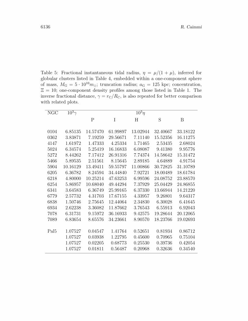
RC, mass logarithm, log(MC/m�), taken from the parent paper [4], are listedin Table 4 together with the inferred inverse fractional distance, γ = rC/RC.The inferred fractional instantaneous tidal radius, η = µ/(1 + µ), for differentdensity profiles among those listed in Table 1, is shown in Table 5, wherethe inverse fractional distance is repeated for better comparison with relatedplots. Concerning Pal5, calculations were performed with regard to fourpossible mass values: for further details and references, an interested reader isaddressed to the parent paper [13].
The location of GCs listed in Table 5 on the (Oγη) plane is shown in Fig. 7for different Galactic density profiles among those listed in Table 1. The regionwhere GCs are bound, according to the assumed formulation of tidal radius,lies above the dotted straight line, η = γ. The inverse fractional distance, γ,related to NGC 5466 and Pal5, is marked by a dotted vertical line.
The above mentioned GCs appear (partially) unbound for all considereddensity profiles, with the possible exception of I. In fact, Pal5 is known to beexperiencing progressive disruption via tidal shoks during disk passages e.g.,[33], [20], and NGC 5466 shows a tidal stream [24], as inferred in an earlierattempt for different formulations of tidal radius [13]. Remaining GCs areplaced inside the stability region, γ < η, with a restricted number close to theboundary, γ = η, for all considered density profiles.
The key parameter, on which the above results mainly depend, is the massof the Galaxy. In fact, a longer Galactic truncation radius implies less amountof mass acting on a selected GC and vice versa. Accordingly, the tidal force isproportional to the Galactic mass and (for unchanged Galactic mass) inverselyproportional to the Galactic truncation radius, as expected.
With regard to the results listed in Table 5 and plotted in Fig. 7, the Galac-tic mass is restricted to stars and gas leaving aside nonbaryonic dark matter.To this respect, the presence of additional mass makes the inverse fractionaldistance, γ, unchanged by definition via Eq. (148), while the fractional tidal ra-dius, η = η+, by definition via Eq. (149), maintains the same formal expressionwhere the mass ratio, µ(ξC − δC), reads:
µ(ξC − δC) =
[1 + ζC
1 + ζG(ξC − δC)
]1/2 [MC
MG(ξC − δC)
]1/2
; (155)
where masses are still restricted to baryonic matter and ζ is the ratio betweennonbaryonic and baryonic mass for a selected subsystem. A constant ratio,ζG(ξC − δC) = ζC = ζ, implies the results are left unchanged in that Eq. (155)reduces to (150).
The above procedure is repeated for two-component embedding spheresconsidered in Subsection 4.2.2 and the results are listed in Table 6 and plottedin Fig. 8.

Gravitational acceleration and tidal effects in special density profiles 6135
Table 4: Parameters of globular clusters studied in an earlier paper [4]. Anadditional cluster, Pal5, considered in a subsequent paper [13] is also includedfor different mass values. Column caption: 1 - name (NGC or Pal); 2 - subsys-tem (A - [Fe/H] > −1, thick disk; B - old halo; C - young halo); 3 - observedradius, rC/pc; 4 - galactocentric distance, RC/kpc; 5 - decimal logarithm ofmass, log φ = log(MC/m�); 6 - inverse fractional distance, γ = rC/RC.
NGC S rCpc
RC
kpclog φ 103γ
0104 A 50.7 7.4 6.16 6.851350362 C 35.7 9.3 5.75 3.838714147 C 34.5 21.3 4.85 1.619725024 C 119.3 18.8 5.91 6.345745272 C 103.0 12.2 5.95 8.442625466 C 101.4 17.2 5.23 5.895355904 C 63.0 6.2 5.91 10.161296205 B 55.4 8.7 5.81 6.367826218 B 21.6 4.5 5.32 4.800006254 B 27.0 4.6 5.38 5.869576341 B 35.0 9.6 5.67 3.645836779 B 25.0 9.7 5.34 2.577326838 A 10.1 6.7 4.61 1.507466934 C 37.5 14.3 5.39 2.622387078 C 65.7 10.4 6.05 6.317317089 B 71.1 10.4 6.00 6.83654
Pal5 C 20 18.6 3.78 1.0752720 18.6 3.65 1.0752720 18.6 3.15 1.0752720 18.6 2.98 1.07527
6136 R. Caimmi
Table 5: Fractional instantaneous tidal radius, η = µ/(1 + µ), inferred forglobular clusters listed in Table 4, embedded within a one-component sphereof mass, MG = 5 · 1010m�; truncation radius; aG = 125 kpc; concentration,Ξ = 10; one-component density profiles among those listed in Table 1. Theinverse fractional distance, γ = rC/RC, is also repeated for better comparisonwith related plots.
NGC 103γ 103η
P I H S B
0104 6.85135 14.57470 61.99897 13.02944 32.40667 33.181220362 3.83871 7.19259 29.56671 7.11140 15.52356 16.112754147 1.61972 1.47333 4.25334 1.71465 2.53435 2.680245024 6.34574 5.25419 16.16833 6.08087 9.41380 9.957765272 8.44262 7.17412 26.91316 7.74374 14.58642 15.314725466 5.89535 2.51561 8.15645 2.89185 4.64889 4.917545904 10.16129 13.49411 59.55797 11.00866 30.72825 31.107896205 6.36782 8.24594 34.44840 7.92721 18.00489 18.617846218 4.80000 10.25214 47.63253 6.99596 24.08752 23.885706254 5.86957 10.68040 49.44294 7.37929 25.04429 24.868556341 3.64583 6.36749 25.99165 6.37330 13.66944 14.212206779 2.57732 4.31703 17.67155 4.33957 9.26801 9.643176838 1.50746 2.75645 12.44064 2.34830 6.30028 6.416456934 2.62238 3.36082 11.87662 3.76543 6.55913 6.920437078 6.31731 9.15972 36.16933 9.42575 19.28644 20.120657089 6.83654 8.65576 34.23661 8.90570 18.23766 19.02693
Pal5 1.07527 0.04547 1.41764 0.52651 0.81934 0.867121.07527 0.03938 1.22795 0.45600 0.70965 0.751041.07527 0.02205 0.68773 0.25530 0.39736 0.420541.07527 0.01811 0.56487 0.20968 0.32636 0.34540

Gravitational acceleration and tidal effects in special density profiles 6137
Table 6: Fractional instantaneous tidal radius, η = µ/(1 + µ), inferred forglobular clusters listed in Table 4, embedded within a two-component (ij)sphere of mass, Mi,G = 1011m�, Mj,G = 1012m�; truncation radius, ai,G = 30kpc, aj,G = 100 kpc; concentration, Ξi = Ξj = 10; two-component densityprofiles considered in Subsection 4.2.2. The inverse fractional distance, γ =rC/RC, is also repeated for better comparison with related plots.
NGC 103γ 103η
PI PS HI HS
0104 6.85135 3.93932 3.39026 4.43380 3.690070362 3.83871 2.27233 1.86155 2.49265 1.976954147 1.61972 0.57317 0.42316 0.58079 0.426205024 6.34574 2.06309 1.52597 2.10705 1.543495272 8.44262 2.59695 2.01639 2.76012 2.089925466 5.89535 0.98317 0.73032 1.01065 0.741375904 10.16129 3.15739 2.81089 3.60758 3.114366205 6.36782 2.49305 2.07314 2.75719 2.217666218 4.80000 1.84201 1.71409 2.11447 1.926986254 5.86957 1.95273 1.81290 2.24338 2.038186341 3.64583 2.04998 1.66786 2.24019 1.765546779 2.57732 1.39733 1.13396 1.52498 1.199046838 1.50746 0.68612 0.60120 0.77926 0.660926934 2.62238 1.27816 0.96695 1.33509 0.990897078 6.31731 3.08644 2.47106 3.34126 2.596057089 6.83654 2.91484 2.33384 3.15573 2.45203
Pal5 1.07527 0.17804 0.13165 0.18190 0.133191.07527 0.15419 0.11401 0.15754 0.115351.07527 0.08631 0.06382 0.08819 0.064571.07527 0.07089 0.05242 0.07243 0.05303

6138 R. Caimmi
An inspection of Table 6 and Fig. 8 discloses that GCs are (partially) un-bound, owing to (i) a less extended inner sphere, and (ii) a massive outersphere. In this view, the presence of tidal tails or tidal streams detected ine.g., NGC 362, NGC 6934, NGC 7078, NGC 7089, [23]; NGC 5904, NGC 6205,[30]; and the above mentioned NGC 5466 [24]; Pal5 [33], [20], should be pre-dicted for the whole amount of Galactic GCs, regardless of tidal shoks duringdisk passages.
The formulation used for the tidal radius relates to a necessary condition,implying GCs above the straight line, η = γ, plotted in Figs. 7-8, could alsobe (partially) unbound.
If a similar amount of fractional dark matter with respect to the Galaxy,Mj,C/Mi,C = 10 in the case under discussion, is considered for each GC andcalculations are repeated, the position on the (Oγη) plane looks similar toFig. 7. In other words, a comparable amount of dark-to-visible mass ratiowithin GCs and the Galaxy makes GCs lie inside or near the stability region,as expected from Eq. (155).
For a generic density profile, g(R) ∝ v2(R)/R via Eqs. (2) and (3) where,in general, v(R) ∝ Rβ hence g(R) ∝ R2β−1 locally. Then no extremum pointfor the gravitational acceleration is expected if β > 1/2, 0 ≤ R ≤ aG, while
the contrary holds if β > 1/2, R>∼ 0, and β < 1/2, R
<∼ aG. For compari-son with the trend inferred from observations, a sample (N = 37) of empiricalrotation curves, v(R), used in a recent investigation [32], is considered. Incom-plete rotation curves lacking data for large (R > 10kpc;N10 = 13) and short(R < 2kpc;N2 = 4) galactocentric distances, are excluded. The resulting sub-sample (N0 = N − N10 − N2 = 20) shows rotation curve slopes substantiallylarger than unity for short galactocentric distances and nearly flat for largegalactocentric distances. If inferred velocities are related to stable circular or-bits, the gravitational acceleration must necessarily exhibit an extremum point(maximum absolute value), which excludes density profiles where no extremumpoint is present, such as H, HI, HS.
6 Conclusion
Homeoidally striated spherical density profiles have been classified with refer-ence to four basic matter distributions, namely (i) isodensity i.e. ρ(r) = const;(ii) isogravity i.e. g(r) = const; (iii) isothermal i.e. v(r) = [GM(r)/r]1/2 =const; (iv) isomass i.e. M(r) = const. In particular, the following densityprofiles have been included: pure power-law; cored power-law; polytropic;Plummer [34], shortened as P; Hernquist [26], shortened as H; Begeman etal. [2], shortened as I; Spano et al. [38], shortened as S; Burkert [5], shortenedas B; for one-component systems, and a few combinations of the above men-
Gravitational acceleration and tidal effects in special density profiles 6139
tioned ones, namely PI, HI, PS, HS, for two-component systems. Special efforthas been devoted to the occurrence of an extremum point in g(r), where thegravitational attraction on a test particle of unit mass attains the maximumabsolute value.
Tidal effects on subsystems have been considered using a definition of tidalradius which is related to a necessary condition. More specifically, given anembedded sphere (subsystem) within an embedding sphere (one-component ortwo-component system), the embedded sphere attains the tidal radius whenthe gravitational force from the embedding and the embedded sphere, on thepoint placed on the boundary of the latter and lying between related centres,are equal in strength but act on opposite sides.
With regard to one-component systems, density profiles currently used forrepresenting galaxies and/or dark matter haloes, among those listed in Table1, have been considered for the embedding sphere. The trend of the fractionalinstantaneous tidal radius, η, vs. the inverse fractional distance, γ, has shownthe stability region, γ < η, is far more extended for density profiles (P, I,S, B) where the gravitational acceleration attains a maximum absolute value,with respect to density profiles (H) where the gravitational acceleration ismonotonically increasing in absolute value. In the former alternative, the tidalradius takes place (γ = η) for two distinct configurations, while in the latteralternative the same holds for a single configuration.
The above mentioned trend is exacerbated for considered two-componentsystems, where PI and PS density profiles exhibit a restricted stability re-gion for embedded spheres, while HI and HS density profiles show no stabilityregion. The gravitational acceleration attains a maximum absolute value inthe former case, while a monotonic behaviour occurs in the latter. The mainfeatures of two-component embedding spheres appear to depend on the innersubsystem, with little effects arising from the outer.
The location of 17 globular clusters studied in earlier attempts [4], [13], forwhich the radius, the mass, and the Galactocentric distance are known, hasbeen shown on the (Oγη) plane for assigned Galactic truncation radius, mass,concentration, and density profiles among those listed in Table 1. Restrictingto star and gas subsystem, sample globular clusters have been found to liewithin the stability region, γ < η, except Pal5 and NGC 5466, which exhibitnoticeable tidal effects e.g., [33], [24]. Taking nonbaryonic dark matter intoconsideration, it has been shown the results remain unchanged in the specialcase where the mass ratio between non baryonic and baryonic matter withinglobular clusters and the Galaxy, at any distance from the centre, attains aconstant value.
On the other hand, all sample globular clusters have been found to lieoutside the stability region if the Galaxy (Mi,G = 1011m�, ai,G = 30 kpc) isembedded within a nonbaryonic dark matter halo (Mj,G = 1012m�, aj,G = 100
6140 R. Caimmi
kpc), for PI, PS, HI, HS, two-component density profiles, unless the dark-to-visible mass ratio within single globular clusters is comparable to its counter-part within the Galaxy.
A comparison of predicted rotation curves, v(R), with a subsample (N0 =20) of empirical rotation curves has shown the occurrence of an extremumpoint (maximum absolute value) in the gravitational acceleration. Accordingly,density profiles where no extremum point takes place, such as H, HI, HS, havenecessarily been excluded.
References
[1] J. An, H. Zhao, Fitting functions for dark matter density profiles,Monthly Notices of the Royal Astronomical Society, 428 (2013), 2805-2811. http://dx.doi.org/10.1093/mnras/sts175
[2] K.G. Begeman, A.H. Broeils, R.H. Sanders, Extended rotation curvesof spiral galaxies: dark haloes and modified dynamics, MonthlyNotices of the Royal Astronomical Society, 249 (1991), 523-537.http://dx.doi.org/10.1093/mnras/249.3.523
[3] L. Bottazzi, Density-scale radius relation in galactic dark halos, unpub-lished bachelor thesis (in Italian), Padua University, 2011.
[4] P. Brosche, M. Odenkirchen, M. Geffert, Instantaneous and average tidalradii of globular clusters, New Astronomy, 4 (1999), 133-139.http://dx.doi.org/10.1016/s1384-1076(99)00014-7
[5] A. Burkert, The Structure of Dark Matter Halos in Dwarf Galaxies, TheAstrophysical Journal, 447 (1995), L25-L28.http://dx.doi.org/10.1086/309560
[6] R. Caimmi, The Potential Energy Tensors for Subsystems. II. Mass Distri-butions with Ellipsoidal, Similar, and Coaxial Strata, The AstrophysicalJournal, 419 (1993), 615-621. http://dx.doi.org/10.1086/173512
[7] R. Caimmi, On bifurcation points in pseudo-barotropes, Acta Cosmolog-ica, XXII (1996), 21-45.
[8] R. Caimmi, The integral Newton’s and MacLaurin’s theorems in tensorform, Astronomische Nachrichten, 324 (2003), 250-264.http://dx.doi.org/10.1002/asna.200310083
[9] R. Caimmi, Holes within galaxies: The egg or the hen?, New Astronomy,13 (2008), 261-284. http://dx.doi.org/10.1016/j.newast.2007.10.005

Gravitational acceleration and tidal effects in special density profiles 6141
[10] R. Caimmi, C. Marmo, The potential-energy tensors for subsystems.: IV.Homeoidally striated density profiles with a central cusp, New Astronomy,8 (2003), 119-140. http://dx.doi.org/10.1016/s1384-1076(02)00197-5
[11] R. Caimmi, C. Marmo, T. Valentinuzzi, A Numerical Fit of Analytical toSimulated Density Profiles in Dark Matter Haloes, Serbian AstronomicalJournal, 170 (2005), 13-32. http://dx.doi.org/10.2298/saj0570013c
[12] R. Caimmi, L. Secco, The potential energy tensors for subsystems, TheAstrophysical Journal, 395 (1992), 119-125.http://dx.doi.org/10.1086/171635
[13] R. Caimmi, L. Secco, A global and a local criterion in definingthe tidal radius, Astronomische Nachrichten, 324 (2003), 491-505.http://dx.doi.org/10.1002/asna.200310158
[14] R. Caimmi, T. Valentinuzzi, The Fractional Virial Potential Energy inTwo-Component Systems, Serbian Astronomical Journal, 177 (2008), 15-38. http://dx.doi.org/10.2298/saj0877015c
[15] C. Carignan, Light and mass distribution of the Magellanic-typespiral NGC 3109, The Astrophysical Journal, 299 (1985), 59-73.http://dx.doi.org/10.1086/163682
[16] S. Chandrasekhar, An Introduction to the Study of the Stellar Structure,Dover Publications, Inc., University of Chicago Press, 1939.
[17] L. Ciotti, Modeling Elliptical Galaxies: Phase-Space Constraints on Two-Component (γ1, γ2) Models, The Astrophysical Journal, 520 (1999), 574-591. http://dx.doi.org/10.1086/307478
[18] L. Ciotti, S. Pellegrini, Self-consistent two-component models of ellipticalgalaxies, Monthly Notices of the Royal Astronomical Society, 255 (1992),561-571. http://dx.doi.org/10.1093/mnras/255.4.561
[19] W. Dehnen, A Family of Potential-Density Pairs for Spherical Galax-ies and Bulges, Monthly Notices of the Royal Astronomical Society, 265(1993), 250-256. http://dx.doi.org/10.1093/mnras/265.1.250
[20] W. Dehnen, M. Odenkirchen, E.K. Grabel, H.-W. Rix, Model-ing the Disruption of the Globular Cluster Palomar 5 by Galac-tic Tides, The Astronomical Journal, 127 (2004), 2753-2770.http://dx.doi.org/10.1086/383214
[21] G. De Vaucouleurs, Recherches sur les Nebuleuses Extragalactiques, An-nales d’Astrophysique, 11 (1948), 247-287.

6142 R. Caimmi
[22] G. Gayda, E.L. Lokas, On the tidal radius of satellites on prograde andretrograde orbits, Arxiv:1508.03149 (2015), 6.
[23] C.J. Grillmair, K.C. Freeman, M. Irwin, P.J. Quinn, Globular Clusterswith Tidal Tails: Deep Two-Color Star Counts, The Astronomical Jour-nal, 109 (1995), 2553-2585. http://dx.doi.org/10.1086/117470
[24] C.J. Grillmair, R. Johnson, The Detection of a 45o Tidal Stream Asso-ciated with the Globular Cluster NGC 5466, The Astrophysical Journal,639 (2006), L17-L20. http://dx.doi.org/10.1086/501439
[25] U. Haud, J. Einasto, Galactic Models with Massive Corona - Part Two -Galaxy, Astronomy & Astrophysics, 223 (1989), 95-106.
[26] L. Hernquist, An analytical model for spherical galaxies and bulges, TheAstrophysical Journal, 356 (1990), 359-364.http://dx.doi.org/10.1086/168845
[27] G.P. Horedt, Polytropes, Astrophysics Space Science Library 306, KluverAcademic Publishers, Dordrecht, 2004.http://dx.doi.org/10.1007/1-4020-2351-0
[28] W. Jaffe, A simple model for the distribution of light in spherical galaxies,Monthly Notices of the Royal Astronomical Society, 202 (1983), 995-999.http://dx.doi.org/10.1093/mnras/202.4.995
[29] J. Kormendy, Brightness distributions in compact and normal galaxies.II - Structure parameters of the spheroidal component, The AstrophysicalJournal, 218 (1977), 333-346. http://dx.doi.org/10.1086/155687
[30] S. Leon, G. Meylan, F. Combes, Tidal tails around 20 Galactic globularclusters: Observational evidence for gravitational disk/bulge shocking,Astronomy & Astrophysics, 359 (2000), 907-931.
[31] W.D. MacMillan, The Theory of the Potential, Dover Publications, NewYork, 1930.
[32] J.H. Marr, Galaxy rotation curves with lognormal density distribution,Monthly Notices of the Royal Astronomical Society, 448 (2015), 3229-3241. http://dx.doi.org/10.1093/mnras/stv216
[33] M. Odenkirchen, E. K. Grebel, W. Dehnen, H.-W. Rix, K. M. Cud-worth, Kinematic Study of the Disrupting Globular Cluster Palomar 5Using VLT Spectra, The Astronomical Journal, 124 (2002), 1497-1510.http://dx.doi.org/10.1086/342287
Gravitational acceleration and tidal effects in special density profiles 6143
[34] H.C. Plummer, On the problem of distribution in globular star clusters,Monthly Notices of the Royal Astronomical Society, 71 (1911), 460-470.http://dx.doi.org/10.1093/mnras/71.5.460
[35] P.H. Roberts, On the Superpotential and Supermatrix of a Hetero-geneous Ellipsoid, The Astrophysical Journal, 136 (1962), 1108-1114.http://dx.doi.org/10.1086/147461
[36] L. Secco, On mechanics and thermodynamics of a stellar galaxy in a two-component virial system and the Fundamental Plane, New Astronomy,10 (2005), 439-461. http://dx.doi.org/10.1016/j.newast.2005.02.003
[37] J.L. Sersic, Influence of the atmospheric and instrumental dispersion onthe brightness distribution in a galaxy, Boletin de la Asociacion Argentinade Astronomia, 6 (1963), 41-43.
[38] M. Spano, M. Marcelin, P. Amram, C. Carignan, B. Epinat, O. Her-nandez et al., GHASP: an H kinematic survey of spiral and irregu-lar galaxies - V. Dark matter distribution in 36 nearby spiral galaxies,Monthly Notices of the Royal Astronomical Society, 383 (2008), 297-316.http://dx.doi.org/10.1111/j.1365-2966.2007.12545.x
[39] N.C. Stone, J. Ostriker, A Dynamical Potential-Density Pair for StarClusters with Nearly Isothermal Interiors, The Astrophysical Journal, 806(2015), L28. http://dx.doi.org/10.1088/2041-8205/806/2/l28
[40] E. Vesperini, On the evolution of the Galactic globular cluster system,Monthly Notices of the Royal Astronomical Society, 287 (1997), 915-928.http://dx.doi.org/10.1093/mnras/287.4.915
[41] S. Von Hoerner, Die Auflosungszeit offener Sternhaufen, Zeitschrift furAstrophysik, 44 (1958), 221-242.
[42] H. Zhao, Analytical models for galactic nuclei, Monthly Notices of theRoyal Astronomical Society, 278 (1996), 488-496.http://dx.doi.org/10.1093/mnras/278.2.488
Appendix
A Homeoidally striated ellipsoidal density pro-
files
Density profiles in dimensionless coordinates, expressed by Eqs. (8)-(9), maybe extended to the case where the isopycnic i.e. constant density surfaces are

6144 R. Caimmi
similar and similarly placed ellipsoids, which implies the dimensionless radialcoordinate, ξ = r(µ)/r†(µ), maintains unchanged on an arbitrary isopycnicsurface, r = r(µ), µ polar angle e.g., [10]. In the special case of homoge-neous ellipsoids, the gravitational potential and force on points not outsidethe ellipsoids are e.g., [12]:
V(x1, x2, x3) = πGρ3∑r=1
Ar(a2r − x2
r) ; (156)
∂V∂xr
= −2πGρArxr ; (157)
where ar are the semiaxes of the ellipsoid and Ar are shape factors for whichthe following inequalities hold e.g., [31] (Chap. II, §33), [7]:
A1 ≤ A2 ≤ A3 ; a1 ≥ a2 ≥ a3 ; (158)
a1A1 ≤ a2A2 ≤ a3A3 ; a1 ≥ a2 ≥ a3 ; (159)
accordingly, the largest gravitational force on the boundary of a homogeneousellipsoid is exerted at the top of the minor axis, P∓ ≡ (0, 0,∓a3). UsingNewton’s theorem, the above result can be extended to a generic inner ellipsoidwith similar and similarly placed boundary.
Turning to the general case of homeoidally striated ellipsoids, let P ≡(x1, x2, x3) be a generic point within the ellipsoid, as represented in Fig. 9.
Owing to Newton’s theorem, no attraction on P is exerted by the homeoidbounded by the external isopycnic surface, Σ(R), and the one where P lies,Σ(r). Then only the ellipsoid bounded by Σ(r) has to be considered.
Let Σ(r) together with all the enclosed isopycnic surfaces be “compressed”along x1 and x2 directions to attain a spherical shape with radius equal to theminor axis of Σ(r), as depicted in Fig. 9. The result is a homeoidally striatedsphere with mass equal to the mass bounded by Σ(r). It is suggested fromgeometrical considerations that the attraction exerted on P by the homeoidallystriated sphere is larger than the attraction exerted on P by the homeoidallystriated ellipsoid.
Let all the isopycnic surfaces within Σ(r) be “stretched” along x1 and x2
directions, with the minor axis left unchanged, to attain a confocal ellipsoidalshape with respect to Σ(r), as depicted in Fig. 9. The result is a focaloidallystriated ellipsoid with mass equal to the mass bounded by Σ(r) and boundaryΣ(r). Let a′′1, a′′2, a′′3, be the semiaxes of a generic isopycnic surface within Σ(r),and a′1, a′2, a′3, the semiaxes of Σ(r). The semiaxes of an ellipsoid internal and
confocal to Σ(r) are c′′r =√
(a′r)2 − λ, where λ is determined by the boundary
condition, c′′3 = a′′3, as λ = (a′3)2 − (a′′3)2. Accordingly, the equatorial semiaxesof the confocal ellipsoid are:
(c′′r)2 = (a′r)
2 − λ = (εr3a′3)2 − (a′3)2 + (a′′3)2 ; (160)
Gravitational acceleration and tidal effects in special density profiles 6145
which is equivalent to:
(c′′r)2 = [(εr3)2 − 1][(a′3)2 − (a′′3)2] + (a′′r)
2 ; (161)
where εr3 = ar/a3 = a′r/a′3 = a′′r/a
′′3, r = 1, 2, are the axis ratios of the isopycnic
surface. As εr3 ≥ 1, a′3 ≥ a′′3, Eq. (161) discloses that, in fact, the equatorialsemiaxes of the confocal ellipsoid are stretched with respect to the equatorialsemiaxes of the related isopycnic surface, c′′r ≥ a′′r , r = 1, 2.
It is suggested from geometrical considerations that the attraction exertedon P by the focaloidally striated ellipsoid is lower than the attraction exertedon P by the homeoidally striated ellipsoid. Owing to MacLaurin’s theorem,the attraction exerted by a focaloidally striated ellipsoid on a surface point, P,equals the attraction exerted on the same point by a homogeneous ellipsoid ofequal mass and boundary.
A homeoidally striated ellipsoid may be conceived as a homogeneous el-lipsoid with equal boundary and density as at the surface isopycnic, to whichis superimposed an infinity of homogeneous ellipsoids bounded by isopycnicsurfaces, Σ(r′′), with infinitesimal density, dρ = ρ(r′′) − ρ(r′′ + dr). Owingto MacLaurin’s theorem, the attraction exerted by the generic homogeneousellipsoid on a surface point, P, equals the attraction exerted by a homoge-neous ellipsoid with equal mass, confocal and confocally placed with respectto the one under consideration, with P on its boundary. The largest attrac-tion exerted on the boundary of a homogeneous ellipsoid is at the top of theminor axis, which implies the largest attraction exerted on the boundary of ahomeoidally striated ellipsoid is also at the top of the minor axis.
For the homeoidally striated sphere, the gravitational attraction along theminor axis, via Eq. (157) keeping in mind Ar = 2/3 for spherical configurations,reads:
∂V∂x3
= −Gm(x3)
x23
; (162)
where m(x3) is the mass of the homeoidally striated ellipsoid enclosed withinthe isopycnic surface with minor axis equal to x3.
For the focaloidally striated ellipsoid, the gravitational attraction along theminor axis, via Eq. (157) reads:
∂V∂x3
= −3
2
Gm(x3)
x23
ε31ε32A3 ; (163)
which is different from its counterpart related to the homeoidally striatedsphere, Eq. (162), by a shape factor, (3/2)ε31ε32A3, as expected.
Accordingly, the extremum point of the radial profile (along the minoraxis) of the attraction i.e. the gravitational acceleration is the same for boththe homeoidally striated sphere and the focaloidally striated ellipsoid, as the

6146 R. Caimmi
two profiles are vertically shifted one with respect to the other, by an amountequal to the shape factor. Then it may safely be expected the extremum pointof the gravitational acceleration, related to the homeoidally striated ellipsoid,is close to its counterpart related to the homeoidally striated sphere and thefocaloidally striated ellipsoid.
B Geometrical interpretation of the dimen-
sionless scaling radius for generalized power
law density profiles
Dimensionless generalized power law density profiles, defined by Eq. (84), indecimal logarithmic scale are expressed as:
log f = log(Cγ + 1) + χ log(Cα + 1)− log(Cγ + ξγ)− χ log(Cα + ξα) ; (164)
where all parameters cannot be negative.The logarithmic derivatives, dn log f/ d(log ξ)n, can be calculated as
[ dn log f/ dξn][ dξ/ d log ξ]n = ξn[ dn log f/ dξn]. For the first, second, third,and fourth derivative, the result is:
d log f
d log ξ= − γξγ
Cγ + ξγ− χαξα
Cα + ξα; (165)
d2 log f
d(log ξ)2= − Cγγ
2ξγ
(Cγ + ξγ)2− χCαα
2ξα
(Cα + ξα)2; (166)
d3 log f
d(log ξ)3= − Cγγ
3ξγ
(Cγ + ξγ)3(Cγ − ξγ)−
χCαα3ξα
(Cα + ξα)3(Cα − ξα) ; (167)
d4 log f
d(log ξ)4= −Cγγ4ξγ
(Cγ − ξγ)2 − 2Cγξγ
(Cγ + ξγ)4− χCαα4ξα
(Cα − ξα)2
(Cα + ξα)4; (168)
and the particularization to the dimensionless scaling radius, ξ = 1, log ξ = 0,yields:[
d log f
d log ξ
]log ξ=0
= − γ
Cγ + 1− χα
Cα + 1; (169)
[d2 log f
d(log ξ)2
]log ξ=0
= − Cγγ2
(Cγ + 1)2− χCαα
2
(Cα + 1)2; (170)
[d3 log f
d(log ξ)3
]log ξ=0
= −Cγγ3(Cγ − 1)
(Cγ + 1)3− χCαα
3
(Cα + 1)3(Cα − 1) ; (171)
[d4 log f
d(log ξ)4
]log ξ=0
= −Cγγ4[(Cγ − 1)2 − 2Cγ]
(Cγ + 1)4− χCαα
4
(Cα + 1)4(Cα − 1)2 ; (172)

Gravitational acceleration and tidal effects in special density profiles 6147
where Eq. (169) coincides with (86), as χα = β − γ by definition.Turning to the general case and keeping in mind all parameters cannot be
negative, the first and the second derivative are always negative while the thirdderivative is null provided the following relation:
Cγγ3ξγ(Cγ − ξγ)
(Cγ + ξγ)3+χCαα
3ξα(Cα − ξα)
(Cα + ξα)3= 0 ; (173)
is satisfied. In particular, Eq. (173) holds at the dimensionless scaling radius,ξ = 1, for Cγ = Cα = 1 (B density profiles); Cγ = 1, Cα = 0 (Z densityprofiles); Cγ = 0, Cα = 1 (Z density profiles). Accordingly, the slope variationrate, d2 log f/ d(log ξ)2, has an extremum point at ξ = 1 where, in addition,the fourth derivative turns out to be positive, which implies the slope variationrate attains a minimum (a maximum in absolute value) at ξ = 1.
Received: September 4, 2015; Published: October 2, 2015

6148 R. Caimmi
Figure 1: The embedding and the embedded sphere, centred in O′ and O,respectively. The minimum gravitational force exerted on the surface of theembedded sphere takes place on P, where the attraction due to each subsystemacts along the same direction but on opposite sides. A null gravitational forceon P defines aC as the tidal radius of the embedded sphere, a∗C, where O movesto O∗ while P remains unchanged. Points mentioned above are represented assaltires. The figure is not in scale for sake of clarity: the embedded sphere,even if the radius equals the tidal radius (dotted), is completely lying withinthe embedding sphere. See text for further details.
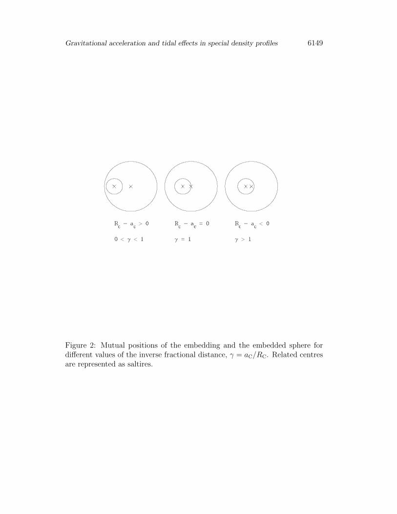
Gravitational acceleration and tidal effects in special density profiles 6149
Figure 2: Mutual positions of the embedding and the embedded sphere fordifferent values of the inverse fractional distance, γ = aC/RC. Related centresare represented as saltires.
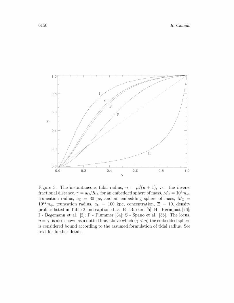
6150 R. Caimmi
Figure 3: The instantaneous tidal radius, η = µ/(µ + 1), vs. the inversefractional distance, γ = aC/RC, for an embedded sphere of mass, MC = 105m�,truncation radius, aC = 30 pc, and an embedding sphere of mass, MG =1012m�, truncation radius, aG = 100 kpc, concentration, Ξ = 10, densityprofiles listed in Table 2 and captioned as: B - Burkert [5]; H - Hernquist [26];I - Begemann et al. [2]; P - Plummer [34]; S - Spano et al. [38]. The locus,η = γ, is also shown as a dotted line, above which (γ < η) the embedded sphereis considered bound according to the assumed formulation of tidal radius. Seetext for further details.

Gravitational acceleration and tidal effects in special density profiles 6151
Figure 4: Zoom of Fig. 3 near the origin. The truncation radius of the em-bedding sphere is attained just after the intersection of related curve with thedotted straight line, η = γ, i.e. just after the tidal radius and the truncationradius of the embedded sphere coincide. The continuation of each curve out-side the truncation radius of the embedding sphere, assuming the continuationof the density profile, is also shown.

6152 R. Caimmi
Figure 5: The instantaneous tidal radius, η = µ/(µ + 1), vs. the inversefractional distance, γ = aC/RC, for an embedded sphere of mass, MC = 105m�,truncation radius, aC = 30 pc, and an embedding two-component sphere ofmass, Mi,G = 1011m�, Mj,G = 1012m�, truncation radius, ai,G = 30 kpc,aj,G = 100 kpc, concentration, Ξi = Ξj = 10, density profiles, ij = PI, PS, HI,HS, captioned as in Fig. 3. Curves related to PI, PS; HI, HS; density profiles,respectively, are nearly coincident and cannot be resolved on the plane of thefigure. The locus, η = γ, is also shown as a dotted line, above which (γ < η) theembedded sphere is considered bound according to the assumed formulationof tidal radius. See text for further details.

Gravitational acceleration and tidal effects in special density profiles 6153
Figure 6: Zoom of Fig. 5 near the origin. The ending point of each curve (left)relates to the truncation radius of the outer embedding sphere (j = I,S), whereγ = 0.0003. The scale has been left unchanged with respect to Fig. 4 for bettercomparison.

6154 R. Caimmi
Figure 7: Location of globular clusters, listed in Table 5, on the (Oγη) plane,for an embedding sphere of mass, MG = 5·1010m�, truncation radius, aG = 125kpc, concentration, Ξ = 10, density profiles among those listed in Table 1,captioned as in Fig. 3. The locus, η = γ, is also shown as an inclined dottedline, above which (γ < η) globular clusters are bound according to the assumedformulation of tidal tadius. The position of NGC 5466 and Pal5, which exhibitnoticeable tidal effects, are marked by vertical dotted lines. See text for furtherdetails.

Gravitational acceleration and tidal effects in special density profiles 6155
Figure 8: Location of globular clusters, listed in Table 6, on the (Oγη) plane,for a two-component embedding sphere of mass, Mi,G = 1011m�, Mj,G =1012m�; truncation radius, ai,G = 30 kpc, aj,G = 100 kpc; concentration,Ξi = Ξj = 10; two-component density profiles considered in Subsection 4.2.2,captioned as in Fig. 5. The locus, η = γ, is also shown as an inclined dottedline, above which (γ < η) globular clusters are bound according to the assumedformulation of tidal tadius. The position of NGC 5466 and Pal5, which exhibitnoticeable tidal effects, are marked by vertical dotted lines. See text for furtherdetails.

6156 R. Caimmi
Figure 9: The attraction exerted by a homeoidally striated ellipsoid on aninternal or surface point, P ≡ (x1, x2, x3), lies between its counterparts relatedto a homeoidally striated sphere and to a focaloidally striated (with respectto the isopycnic surface passing through P) ellipsoid where, in both cases,isopycnic surfaces tangent at the minor axis enclose an equal mass, m(x3).See text for further details. The outer ellipsoid represents the boundary ofthe homeoidally striated ellipsoid, Σ(R). The inner ellipsoid represents theisopycnic surface of the homeoidally striated ellipsoid, Σ(r), passing throughP, also shown (cross). The sphere represents the isopycnic surface of thehomeoidally striated sphere, enclosing the same mass as Σ(r). The horizontalbar represents the focal ellipse with respect to the focaloidally striated ellipsoid,enclosing the same mass as the central isopycnic surface of the homeoidallystriated ellipsoid (saltire). The coordinate axes, x1 and x2, are not drawn toavoid confusion.