graphs an introduction. ouline what are graphs? applications terminology and problems representation...
Post on 20-Dec-2015
216 views
TRANSCRIPT

Graphs
An Introduction

Ouline
• What are Graphs?• Applications• Terminology and Problems• Representation (Adj. Mat and Linked
Lists)• Searching
– Depth First Search (DFS)– Breadth First Search (BFS)

Graphs
• A graph G = (V,E) is composed of:– V: set of vertices– E V V: set of edges connecting
the vertices
• An edge e = (u,v) is a __ pair of vertices– Directed graphs (ordered pairs)– Undirected graphs (unordered pairs)

Directed graph

Directed Graph

Undirected GRAPH
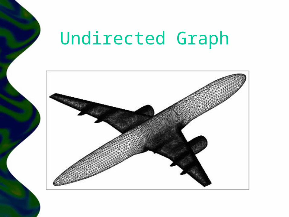
Undirected Graph

Applications
• Air Flights, Road Maps, Transportation.
• Graphics / Compilers• Electrical Circuits• Networks• Modeling any kind of relationships
(between people/web pages/cities/…)
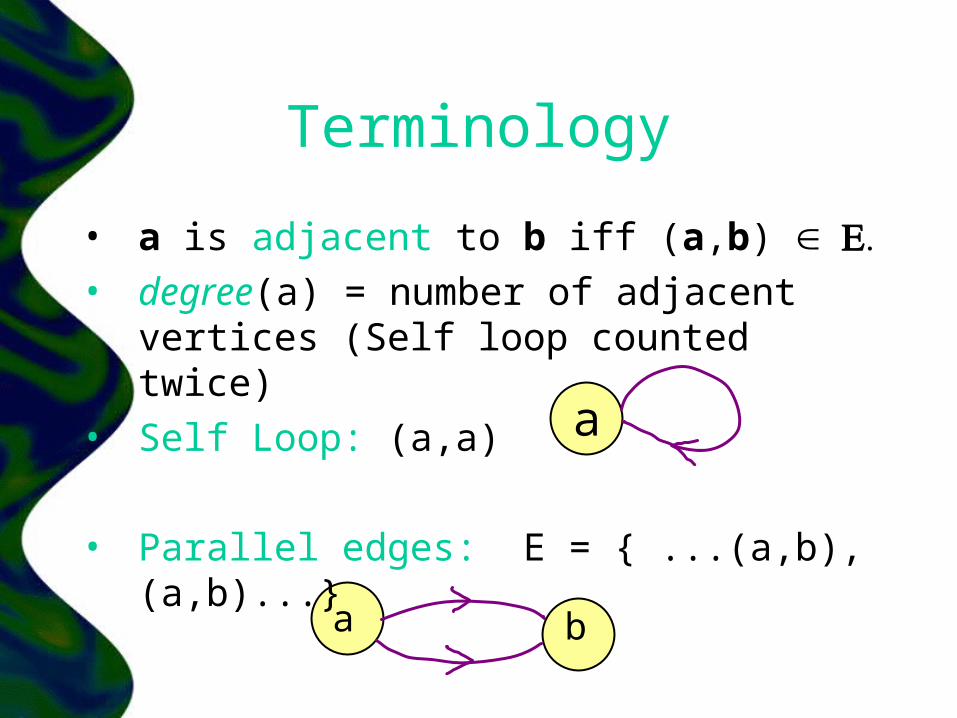
Terminology
• a is adjacent to b iff (a,b) • degree(a) = number of adjacent
vertices (Self loop counted twice)• Self Loop: (a,a)
• Parallel edges: E = { ...(a,b), (a,b)...}
a
a b

Terminology
• A Simple Graph is a graph with no self loops or parallel edges.
• Incidence: v is incident to e if v is an end vertex of e.
ve

More…
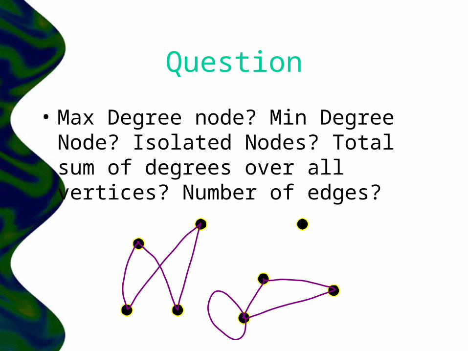
Question
• Max Degree node? Min Degree Node? Isolated Nodes? Total sum of degrees over all vertices? Number of edges?
Question
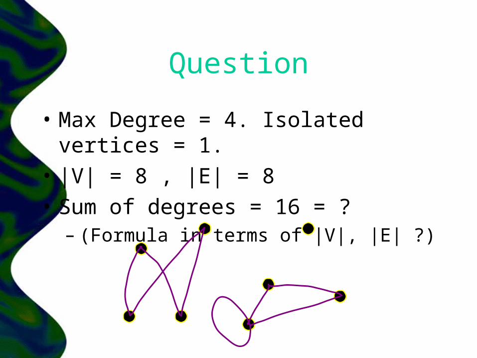
• Max Degree = 4. Isolated vertices = 1.
• |V| = 8 , |E| = 8• Sum of degrees = 16 = ?
– (Formula in terms of |V|, |E| ?)
Question
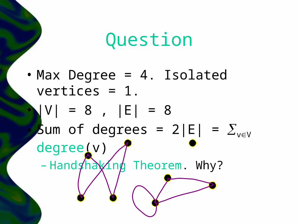
• Max Degree = 4. Isolated vertices = 1.
• |V| = 8 , |E| = 8
• Sum of degrees = 2|E| = vV degree(v)– Handshaking Theorem. Why?

QUESTION
• How many edges are there in a graph with 100 vertices each of degree 4?
QUESTION
• How many edges are there in a graph with 100 vertices each of degree 4?– Total degree sum = 400 = 2 |E|– 200 edges by the handshaking
theorem.

Handshaking:CorollaryThe number of vertices with odd degree is
always even.Proof: Let V1 and V2 be the set of vertices
of even and odd degrees, respectively (Hence V1 V2 = , and V1 V2 = V).
• Now we know that
2|E| = vV degree(v)
= vV1 degree(v) + vV2 degree(v)
• Since degree(v) is odd for all v V2, | V2 | must be even.

Terminology
Path and Cycle
• An alternating sequence of vertices and edges beginning and ending with vertices – each edge is incident with the vertices
preceding and following it.– No edge / vertex appears more than once.
• Cycle– A path is a cycle if and only if v0= vk
• The beginning and end are the same vertex.

Path example

Connected graph
• Undirected Graphs: If there is at least one path between every pair of vertices. (otherwise disconnected)
• Directed Graphs:– Strongly connected– Weakly connected

hamiltonian cycle
• Closed cycle that transverses every vertex exactly once.
In general, the problem of finding a Hamiltonian circuit
is NP-Complete.
complete graph
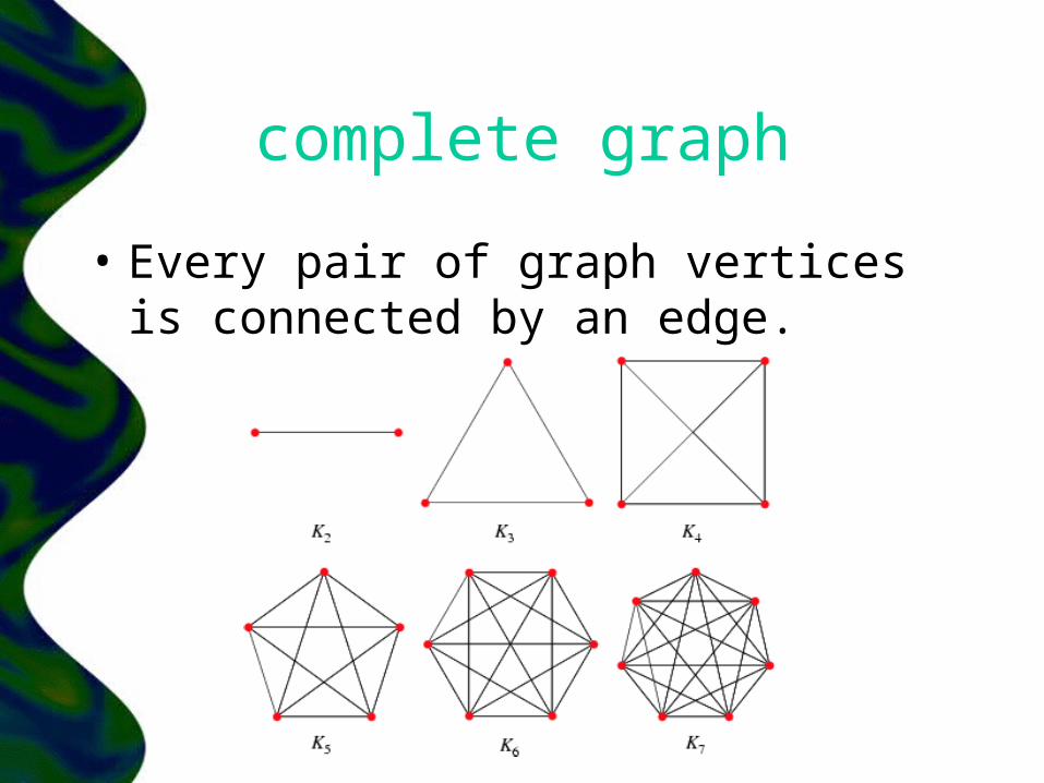
• Every pair of graph vertices is connected by an edge.

Directed Acyclic Graphs• A DAG is a directed graph with no cycles
• Often used to indicate precedences among events, i.e., event a must happen before b
• Where have we seen these graphs before?

Tree
A connected graph with n nodes and n-1 edges
A Forest is a collection of trees.
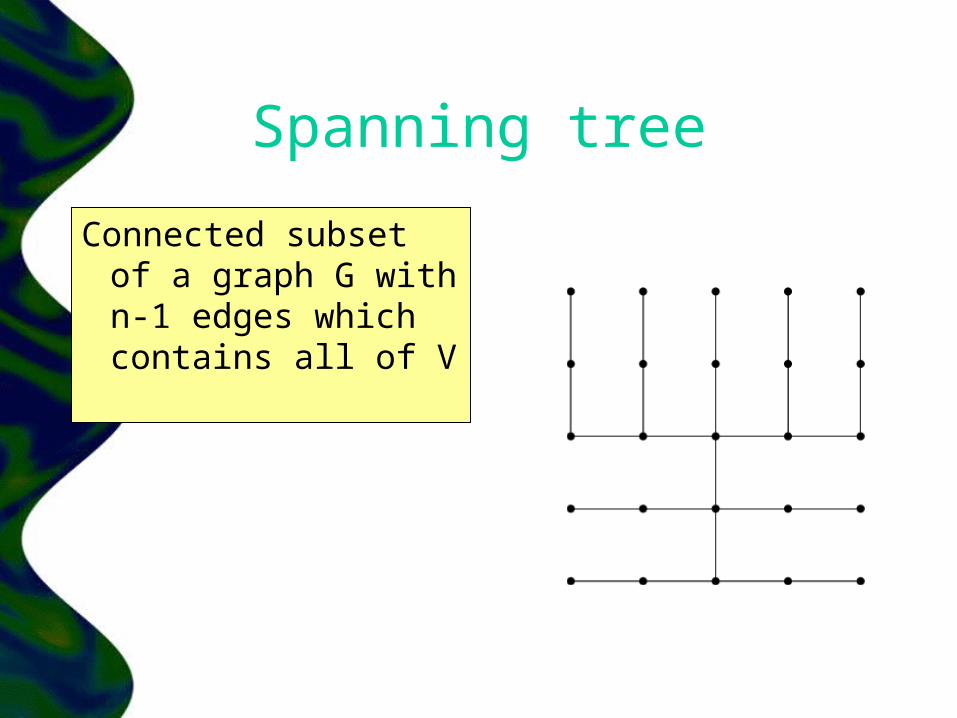
Spanning tree
Connected subset of a graph G with n-1 edges which contains all of V

independent set
• An independent set of G is a subset of the vertices such that no two vertices in the subset are adjacent.

cliques
• a.k.a. complete subgraphs.

tough Problem
• Find the maximum cardinality independent set of a graph G. – NP-Complete
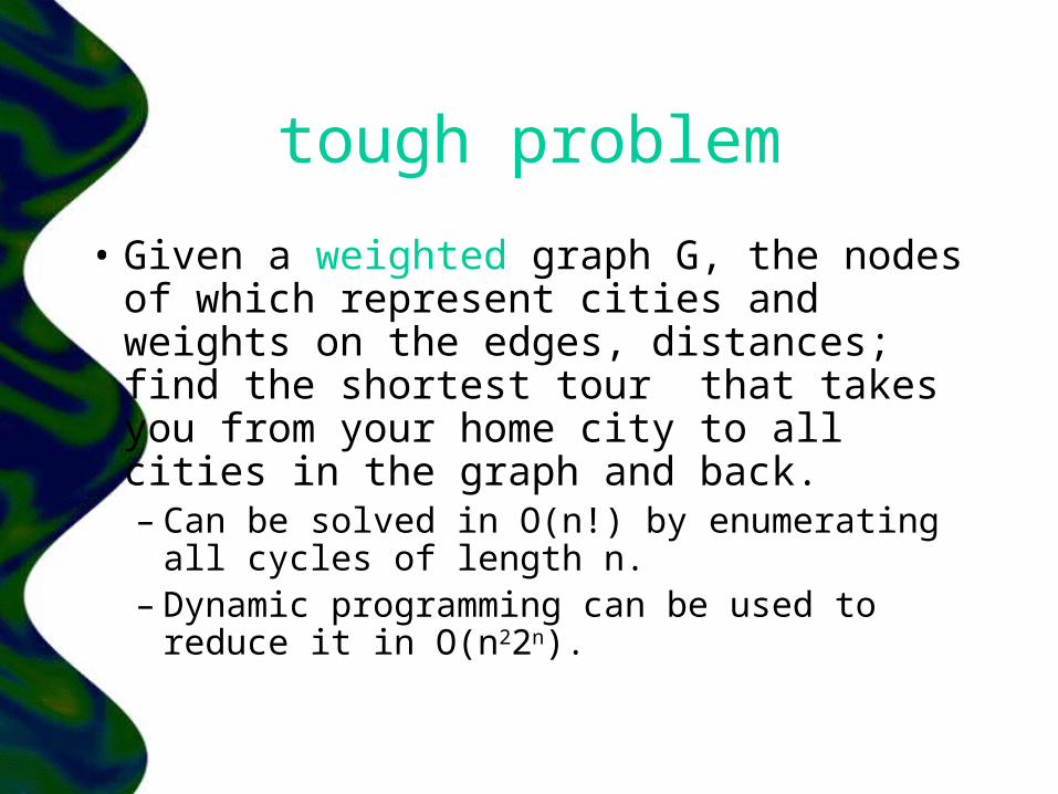
tough problem
• Given a weighted graph G, the nodes of which represent cities and weights on the edges, distances; find the shortest tour that takes you from your home city to all cities in the graph and back.– Can be solved in O(n!) by enumerating
all cycles of length n.– Dynamic programming can be used to
reduce it in O(n22n).

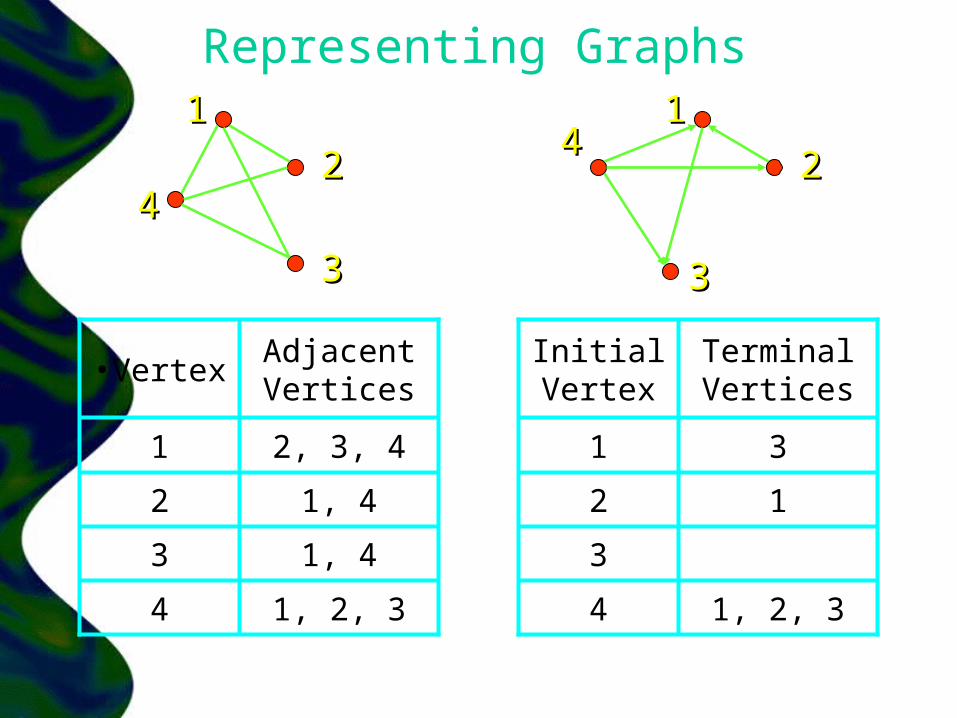
representation
• Two ways– Adjacency List
• ( as a linked list for each node in the graph to represent the edges)
– Adjacency Matrix• (as a boolean matrix)
Representing Graphs11
22
33
44
11
22
33
44
1, 42
1, 43
1, 2, 34
2, 3, 41
Adjacent Vertices
•Vertex
12
3
1, 2, 34
31
Terminal Vertices
Initial Vertex

adjacency list

adjacency matrix

Another example
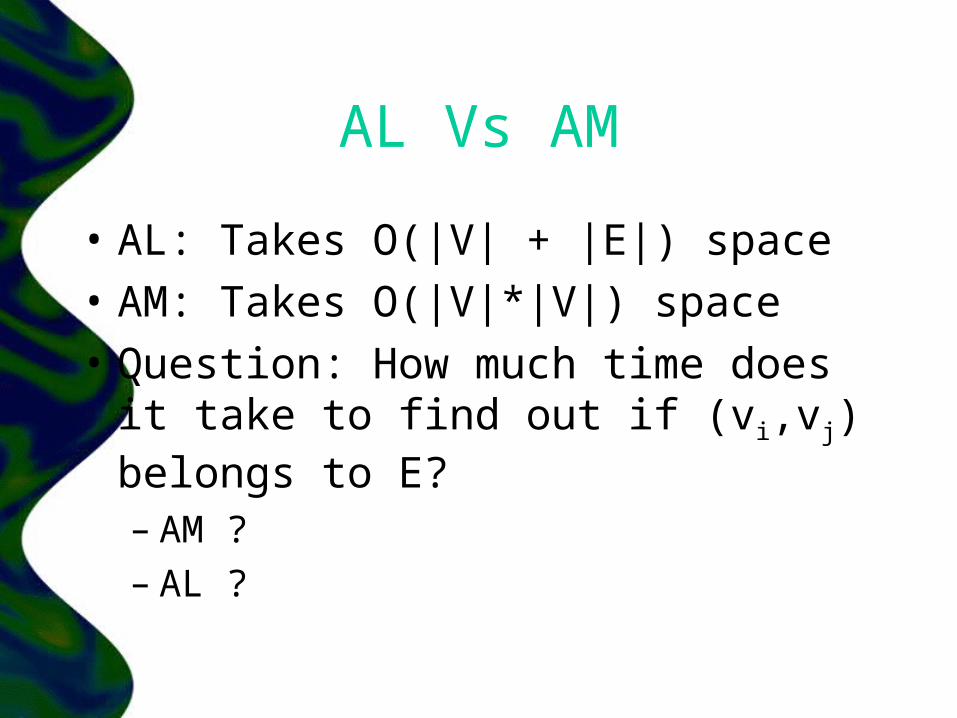
AL Vs AM
• AL: Takes O(|V| + |E|) space• AM: Takes O(|V|*|V|) space• Question: How much time does it
take to find out if (vi,vj) belongs to E?– AM ?– AL ?

AL Vs AM
• AL: Takes O(|V| + |E|) space• AM: Takes O(|V|*|V|) space• Question: How much time does it
take to find out if (vi,vj) belongs to E?– AM : O(1)– AL : O(|V|) in the worst case.

AL Vs AM
• AL : Total space = 4|V| + 8|E| bytes (For undirected graphs its 4|V| + 16|E| bytes)
• AM : |V| * |V| / 8
• Question: What is better for very sparse graphs? (Few number of edges)

BFS/DFS
© Steve Skiena
BFS : Breadth First Search
DFS : Depth First Search
BFS/DFS
• Breadth-first search (BFS) and depth-first search (DFS) are two distinct orders in which to visit the vertices and edges of a graph.
• BFS: radiates out from a root to visit vertices in order of their distance from the root. Thus closer nodes get visited first.

Breadth first search
• Question: Given G in AM form, how do we say if there is a path between nodes a and b?
• Note: Using AM or AL its easy to answer if there is an edge (a,b) in the graph, but not path questions. This is one of the reasons to learn BFS/DFS.

BFS
• A Breadth-First Search (BFS) traverses a connected component of a graph, and in doing so defines a spanning tree.
Source: Lecture notes by Sheung-Hung POON

BFS
Example
2
4
3
5
1
76
9
8
0
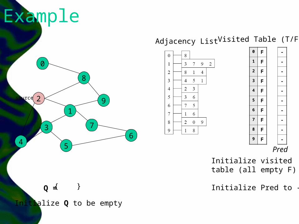
Adjacency List
source
0
1
2
3
4
5
6
7
8
9
Visited Table (T/F)
F
F
F
F
F
F
F
F
F
F
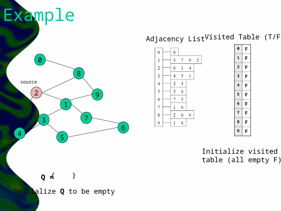
Q = { }
Initialize visitedtable (all empty F)
Initialize Q to be empty

Example
2
4
3
5
1
76
9
8
0
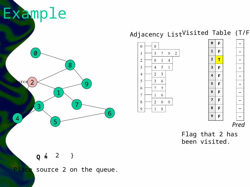
Adjacency List
source
0
1
2
3
4
5
6
7
8
9
Visited Table (T/F)
F
F
T
F
F
F
F
F
F
F
Q = { 2 }
Flag that 2 has been visited.
Place source 2 on the queue.
Example
2
4
3
5
1
76
9
8
0
Adjacency List
source
0
1
2
3
4
5
6
7
8
9
Visited Table (T/F)
F
T
T
F
T
F
F
F
T
F
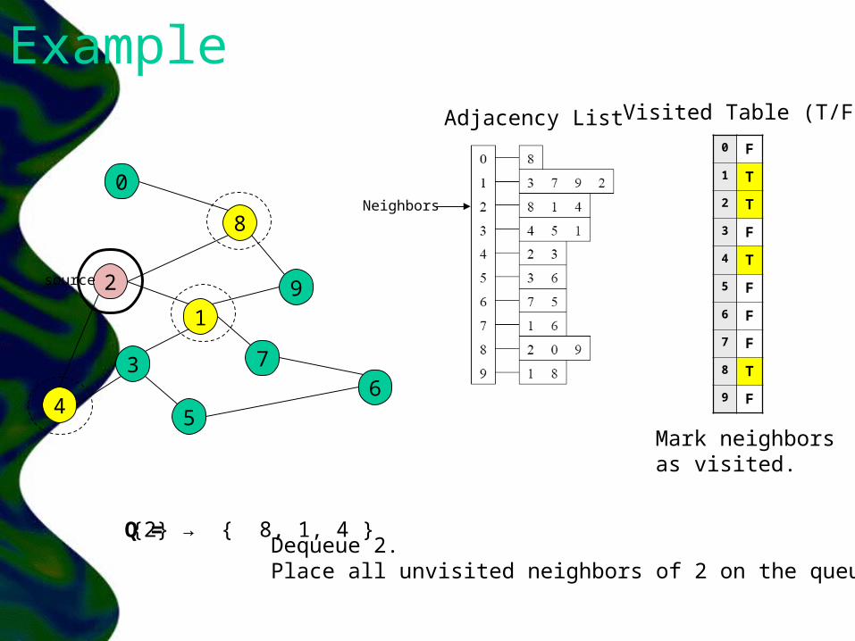
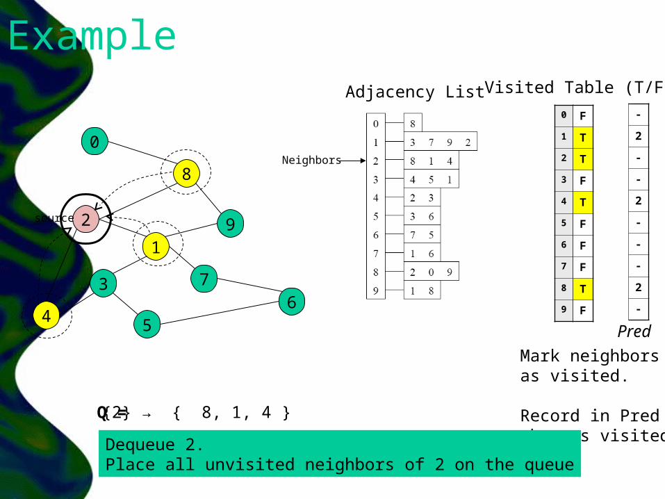
Q = {2} → { 8, 1, 4 }
Mark neighborsas visited.
Dequeue 2. Place all unvisited neighbors of 2 on the queue
Neighbors

Example
2
4
3
5
1
76
9
8
0
Adjacency List
source
0
1
2
3
4
5
6
7
8
9
Visited Table (T/F)
T
T
T
F
T
F
F
F
T
T
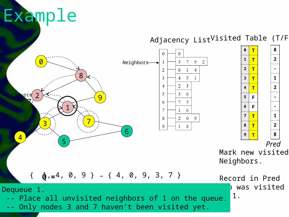
Q = { 8, 1, 4 } → { 1, 4, 0, 9 }
Mark new visitedNeighbors.
Dequeue 8. -- Place all unvisited neighbors of 8 on the queue. -- Notice that 2 is not placed on the queue again, it has been visited!
Neighbors

Example
2
4
3
5
1
76
9
8
0
Adjacency List
source
0
1
2
3
4
5
6
7
8
9
Visited Table (T/F)
T
T
T
T
T
F
F
T
T
T
Q = { 1, 4, 0, 9 } → { 4, 0, 9, 3, 7 }
Mark new visitedNeighbors.
Dequeue 1. -- Place all unvisited neighbors of 1 on the queue. -- Only nodes 3 and 7 haven’t been visited yet.
Neighbors

Example
2
4
3
5
1
76
9
8
0
Adjacency List
source
0
1
2
3
4
5
6
7
8
9
Visited Table (T/F)
T
T
T
T
T
F
F
T
T
T
Q = { 4, 0, 9, 3, 7 } → { 0, 9, 3, 7 } Dequeue 4. -- 4 has no unvisited neighbors!
Neighbors

Example
2
4
3
5
1
76
9
8
0
Adjacency List
source
0
1
2
3
4
5
6
7
8
9
Visited Table (T/F)
T
T
T
T
T
F
F
T
T
T
Q = { 0, 9, 3, 7 } → { 9, 3, 7 } Dequeue 0. -- 0 has no unvisited neighbors!
Neighbors

Example
2
4
3
5
1
76
9
8
0
Adjacency List
source
0
1
2
3
4
5
6
7
8
9
Visited Table (T/F)
T
T
T
T
T
F
F
T
T
T
Q = { 9, 3, 7 } → { 3, 7 } Dequeue 9. -- 9 has no unvisited neighbors!
Neighbors

Example
2
4
3
5
1
76
9
8
0
Adjacency List
source
0
1
2
3
4
5
6
7
8
9
Visited Table (T/F)
T
T
T
T
T
T
F
T
T
T
Q = { 3, 7 } → { 7, 5 } Dequeue 3.
-- place neighbor 5 on the queue.
Neighbors
Mark new visitedVertex 5.

Example
2
4
3
5
1
76
9
8
0
Adjacency List
source
0
1
2
3
4
5
6
7
8
9
Visited Table (T/F)
T
T
T
T
T
T
T
T
T
T
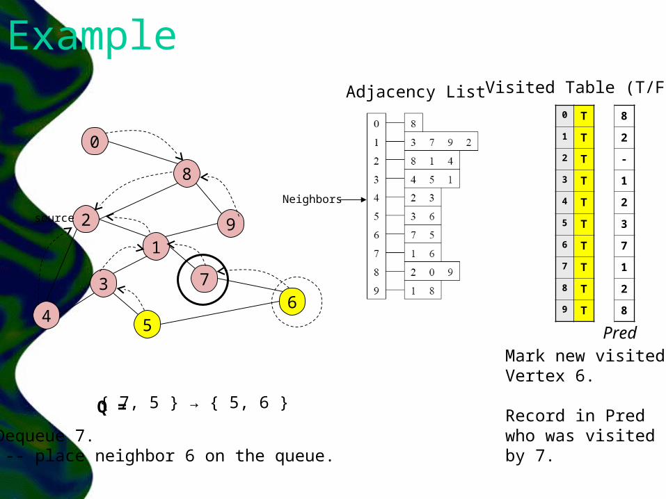
Q = { 7, 5 } → { 5, 6 } Dequeue 7. -- place neighbor 6 on the queue.
Neighbors
Mark new visitedVertex 6.

Example
2
4
3
5
1
76
9
8
0
Adjacency List
source
0
1
2
3
4
5
6
7
8
9
Visited Table (T/F)
T
T
T
T
T
T
T
T
T
T
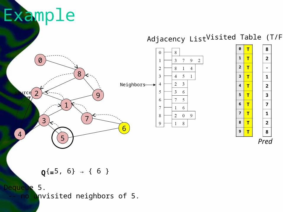
Q = { 5, 6} → { 6 } Dequeue 5. -- no unvisited neighbors of 5.
Neighbors

Example
2
4
3
5
1
76
9
8
0
Adjacency List
source
0
1
2
3
4
5
6
7
8
9
Visited Table (T/F)
T
T
T
T
T
T
T
T
T
T
Q = { 6 } → { } Dequeue 6. -- no unvisited neighbors of 6.
Neighbors

Example
2
4
3
5
1
76
9
8
0
Adjacency List
source
0
1
2
3
4
5
6
7
8
9
Visited Table (T/F)
T
T
T
T
T
T
T
T
T
T
Q = { }
STOP!!! Q is empty!!!
Neighbors
What did we discover?
Look at “visited” tables.
There exist a path from sourcevertex 2 to all vertices in the graph!
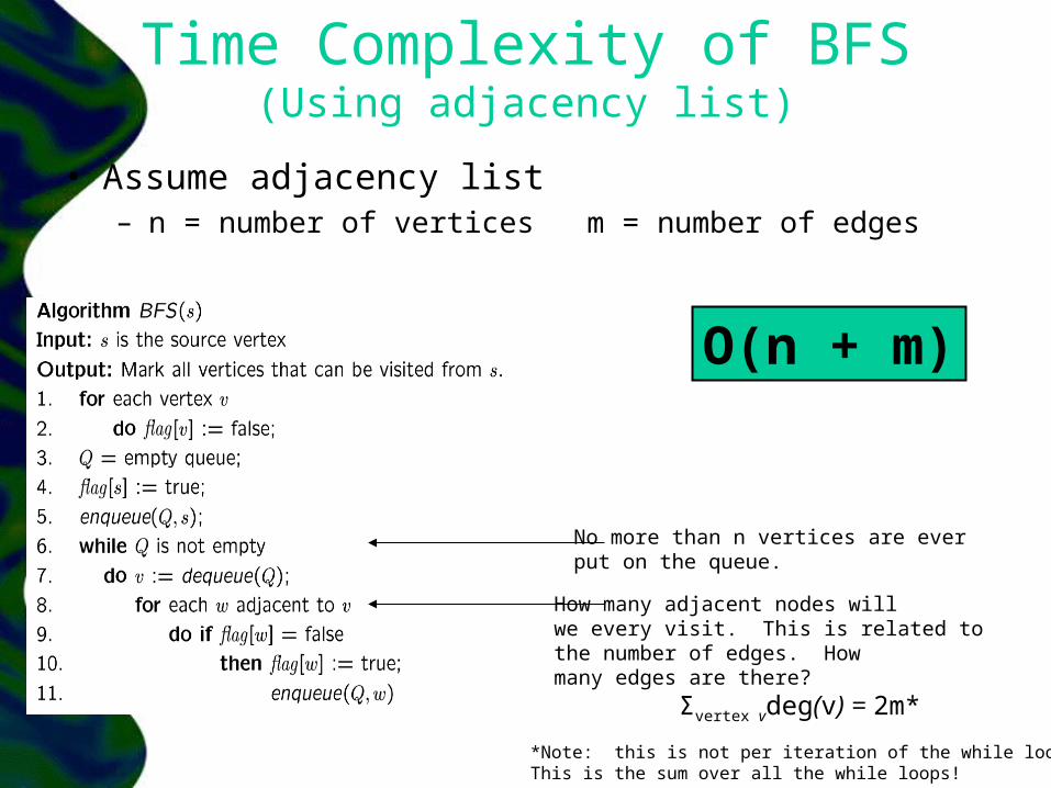
Time Complexity of BFS(Using adjacency list)
• Assume adjacency list– n = number of vertices m = number of edges
Σvertex vdeg(v) = 2m*
No more than n vertices are everput on the queue.
How many adjacent nodes willwe every visit. This is related tothe number of edges. Howmany edges are there?
*Note: this is not per iteration of the while loop.This is the sum over all the while loops!
O(n + m)

Time Complexity of BFS(Using adjacency matrix)
• Assume adjacency list– n = number of vertices m = number of edges
No more than n vertices are everput on the queue. O(n)
Using an adjacency matrix. To findthe neighbors we have to visit all elementsIn the row of v. That takes constant timeO(n)!
O(n2)So, adjacency matrix is not good for BFS!!!

Path Recording
• BFS only tells us if a path exists from source s, to other vertices v.– It doesn’t tell us the path!– We need to modify the algorithm to record the
path.
• Not difficult– Use an additional predecessor array pred[0..n-
1]– Pred[w] = v
• Means that vertex w was visited by v

BFS + Path Finding
Set pred[v] to -1 (let -1 means no path to any vertex)
Record who visited w
Example
2
4
3
5
1
76
9
8
0
Adjacency List
source
0
1
2
3
4
5
6
7
8
9
Visited Table (T/F)
F
F
F
F
F
F
F
F
F
F
Q = { }
Initialize visitedtable (all empty F)
Initialize Pred to -1
Initialize Q to be empty
-
-
-
-
-
-
-
-
-
-
Pred
Example
2
4
3
5
1
76
9
8
0
Adjacency List
source
0
1
2
3
4
5
6
7
8
9
Visited Table (T/F)
F
F
T
F
F
F
F
F
F
F
Q = { 2 }
Flag that 2 has been visited.
Place source 2 on the queue.
-
-
-
-
-
-
-
-
-
-
Pred
Example
2
4
3
5
1
76
9
8
0
Adjacency List
source
0
1
2
3
4
5
6
7
8
9
Visited Table (T/F)
F
T
T
F
T
F
F
F
T
F
Q = {2} → { 8, 1, 4 }
Mark neighborsas visited.
Record in Predwho was visitedby 2.
Dequeue 2. Place all unvisited neighbors of 2 on the queue
Neighbors
-
2
-
-
2
-
-
-
2
-
Pred

Example
2
4
3
5
1
76
9
8
0
Adjacency List
source
0
1
2
3
4
5
6
7
8
9
Visited Table (T/F)
T
T
T
F
T
F
F
F
T
T
Q = { 8, 1, 4 } → { 1, 4, 0, 9 }
Dequeue 8. -- Place all unvisited neighbors of 8 on the queue. -- Notice that 2 is not placed on the queue again, it has been visited!
Neighbors
8
2
-
-
2
-
-
-
2
8
PredMark new visitedNeighbors.
Record in Predwho was visitedby 8.
Example
2
4
3
5
1
76
9
8
0
Adjacency List
source
0
1
2
3
4
5
6
7
8
9
Visited Table (T/F)
T
T
T
T
T
F
F
T
T
T
Q = { 1, 4, 0, 9 } → { 4, 0, 9, 3, 7 }
Mark new visitedNeighbors.
Record in Predwho was visitedby 1.
Dequeue 1. -- Place all unvisited neighbors of 1 on the queue. -- Only nodes 3 and 7 haven’t been visited yet.
Neighbors
8
2
-
1
2
-
-
1
2
8
Pred

Example
2
4
3
5
1
76
9
8
0
Adjacency List
source
0
1
2
3
4
5
6
7
8
9
Visited Table (T/F)
T
T
T
T
T
F
F
T
T
T
Q = { 4, 0, 9, 3, 7 } → { 0, 9, 3, 7 }
Dequeue 4. -- 4 has no unvisited neighbors!
Neighbors
8
2
-
1
2
-
-
1
2
8
Pred

Example
2
4
3
5
1
76
9
8
0
Adjacency List
source
0
1
2
3
4
5
6
7
8
9
Visited Table (T/F)
T
T
T
T
T
F
F
T
T
T
Q = { 0, 9, 3, 7 } → { 9, 3, 7 }
Dequeue 0. -- 0 has no unvisited neighbors!
Neighbors
8
2
-
1
2
-
-
1
2
8
Pred

Example
2
4
3
5
1
76
9
8
0
Adjacency List
source
0
1
2
3
4
5
6
7
8
9
Visited Table (T/F)
T
T
T
T
T
F
F
T
T
T
Q = { 9, 3, 7 } → { 3, 7 }
Dequeue 9. -- 9 has no unvisited neighbors!
Neighbors
8
2
-
1
2
-
-
1
2
8
Pred

Example
2
4
3
5
1
76
9
8
0
Adjacency List
source
0
1
2
3
4
5
6
7
8
9
Visited Table (T/F)
T
T
T
T
T
T
F
T
T
T
Q = { 3, 7 } → { 7, 5 }
Dequeue 3. -- place neighbor 5 on the queue.
Neighbors
Mark new visitedVertex 5.
Record in Predwho was visitedby 3.
8
2
-
1
2
3
-
1
2
8
Pred
Example
2
4
3
5
1
76
9
8
0
Adjacency List
source
0
1
2
3
4
5
6
7
8
9
Visited Table (T/F)
T
T
T
T
T
T
T
T
T
T
Q = { 7, 5 } → { 5, 6 }
Dequeue 7. -- place neighbor 6 on the queue.
Neighbors
Mark new visitedVertex 6.
Record in Predwho was visitedby 7.
8
2
-
1
2
3
7
1
2
8
Pred
Example
2
4
3
5
1
76
9
8
0
Adjacency List
source
0
1
2
3
4
5
6
7
8
9
Visited Table (T/F)
T
T
T
T
T
T
T
T
T
T
Q = { 5, 6} → { 6 }
Dequeue 5. -- no unvisited neighbors of 5.
Neighbors
8
2
-
1
2
3
7
1
2
8
Pred

Example
2
4
3
5
1
76
9
8
0
Adjacency List
source
0
1
2
3
4
5
6
7
8
9
Visited Table (T/F)
T
T
T
T
T
T
T
T
T
T
Q = { 6 } → { }
Dequeue 6. -- no unvisited neighbors of 6.
Neighbors
8
2
-
1
2
3
7
1
2
8
Pred

Example
2
4
3
5
1
76
9
8
0
Adjacency List
source
0
1
2
3
4
5
6
7
8
9
Visited Table (T/F)
T
T
T
T
T
T
T
T
T
T
Q = { }
STOP!!! Q is empty!!!
Neighbors
Pred now stores the path!
8
2
-
1
2
3
7
1
2
8
Pred

Pred array represents paths8
2
-
1
2
3
7
1
2
8
0
1
2
3
4
5
6
7
8
9
nodes visited by
Try some examples.Path(0) ->Path(6) ->Path(1) ->

BFS tree
• We often draw the BFS paths are a m-ary tree, where s is the root.
Question: What would a “level” order traversal tell you?

More onPaths and trees
in graphs
BFS
• Another way to think of the BFS tree is the physical analogy of the BFS Tree.
• Sphere-String Analogy : Think of the nodes as spheres and edges as unit length strings. Lift the sphere for vertex s.

Sphere-String Analogy
bfs : Properties
• At some point in the running of BFS, Q only contains vertices/nodes at layer d.
• If u is removed before v in BFS then– dist(u) dist(v)
• At the end of BFS, for each vertex v reachable from s, the dist(v) equals the shortest path length from s to v.

BFS

BFS:advancing wavefront
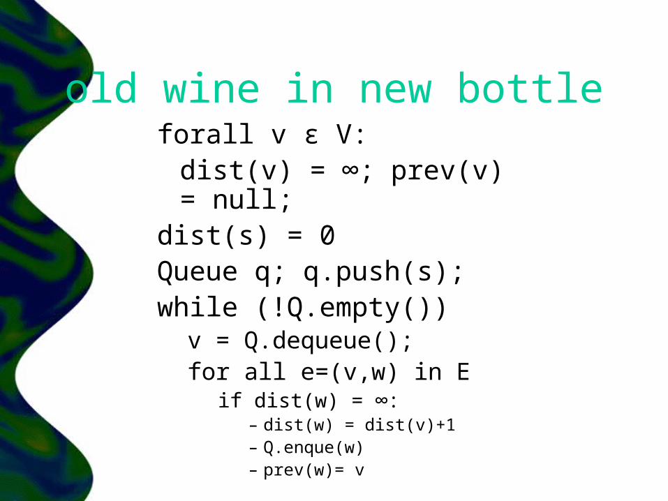
old wine in new bottleforall v ε V:
dist(v) = ∞; prev(v) = null;
dist(s) = 0Queue q; q.push(s);while (!Q.empty())
v = Q.dequeue();for all e=(v,w) in E
if dist(w) = ∞: – dist(w) = dist(v)+1– Q.enque(w)– prev(w)= v
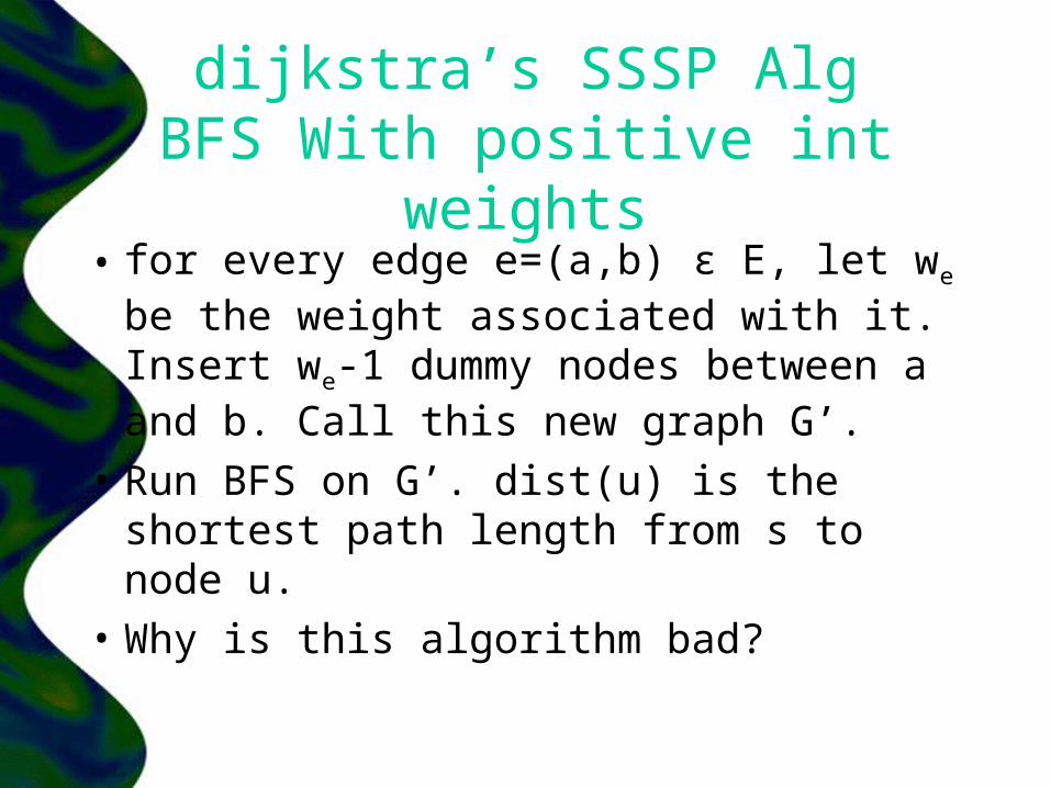
dijkstra’s SSSP AlgBFS With positive int weights
• for every edge e=(a,b) ε E, let we be the weight associated with it. Insert we-1 dummy nodes between a and b. Call this new graph G’.
• Run BFS on G’. dist(u) is the shortest path length from s to node u.
• Why is this algorithm bad?

how do we speed it up?
• If we could run BFS without actually creating G’, by somehow simulating BFS of G’ on G directly.
• Solution: Put a system of alarms on all the nodes. When the BFS on G’ reaches a node of G, an alarm is sounded. Nothing interesting can happen before an alarm goes off.

an example

Another Example

alarm clock alg
alarm(s) = 0until no more alarms
– wait for an alarm to sound. Let next alarm that goes off is at node v at time t.• dist(s,v) = t• for each neighbor w of v in G:
– If there is no alarm for w, alarm(w) = t+weight(v,w)
– If w’s alarm is set further in time than t+weight(v,w), reset it to t+weight(v,w).

recall bfsforall v ε V:
dist(v) = ∞; prev(v) = null;
dist(s) = 0Queue q; q.push(s);while (!Q.empty())
v = Q.dequeue();for all e=(v,w) in E
if dist(w) = ∞: – dist(w) = dist(w)+1– Q.enque(w)– prev(w)= v
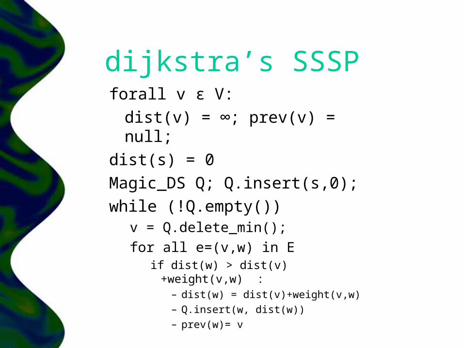
dijkstra’s SSSPforall v ε V:
dist(v) = ∞; prev(v) = null;dist(s) = 0Magic_DS Q; Q.insert(s,0);while (!Q.empty())
v = Q.delete_min();for all e=(v,w) in E
if dist(w) > dist(v)+weight(v,w) :
– dist(w) = dist(v)+weight(v,w)– Q.insert(w, dist(w))– prev(w)= v
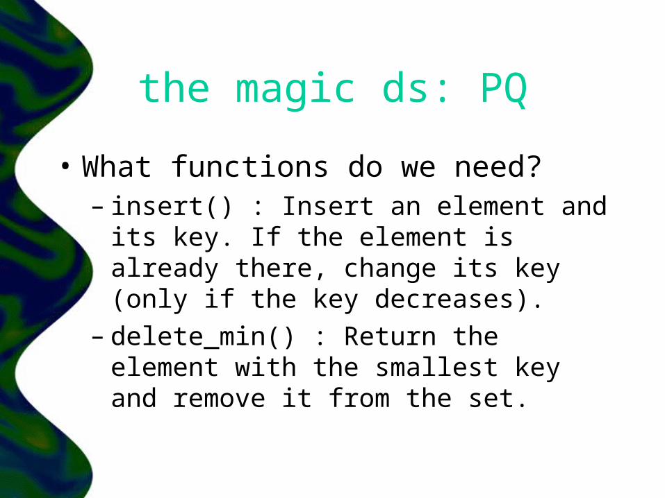
the magic ds: PQ
• What functions do we need?– insert() : Insert an element and its
key. If the element is already there, change its key (only if the key decreases).
– delete_min() : Return the element with the smallest key and remove it from the set.

Example
0
s
u v
x y
10
1
9
2
4 6
5
2 3
7

Example
0
5
10
s
u v
x y
10
1
9
2
4 6
5
2 3
7

Example
0
75
148
s
u v
x y
10
1
9
2
4 6
5
2 3
7

Example
0
75
138
s
u v
x y
10
1
9
2
4 6
5
2 3
7

Example
0
75
98
s
u v
x y
10
1
9
2
4 6
5
2 3
7
Example
0
75
98
s
u v
x y
10
1
9
2
4 6
5
2 3
7

another view region growth
1. Start from s2. Grow a region R around s such
that the SPT from s is known inside the region.
3. Add v to R such that v is the closest node to s outside R.
4. Keep building this region till R = V.
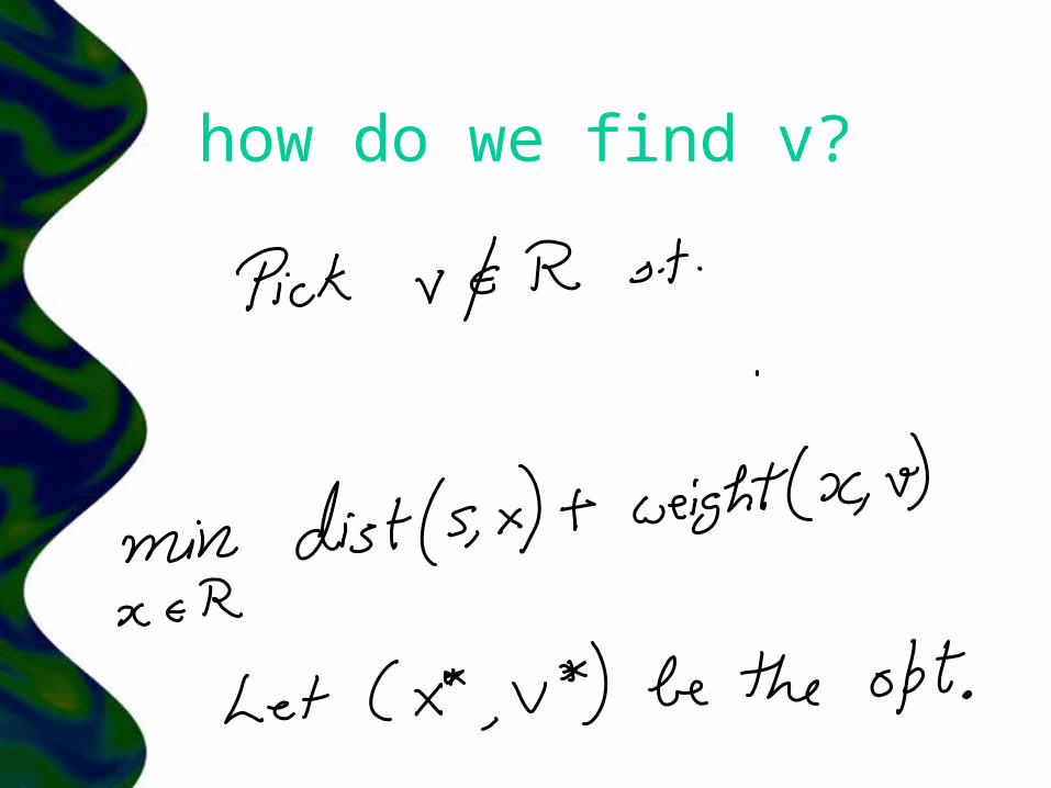
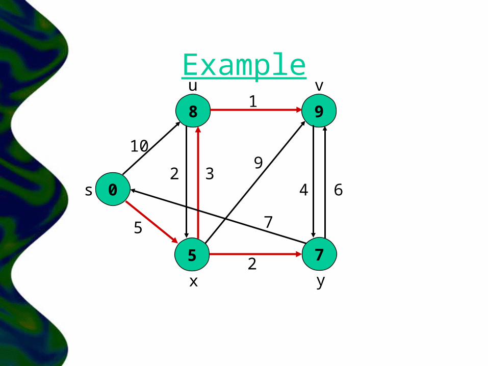
how do we find v?

Example

S,V
Is this the shortest path to V

old wine in new bottleforall v ε V:
dist(v) = ∞; prev(v) = null;dist(s) = 0R = {};while R != V
Pick v not in R with smallest distance to sfor all edges (v,z) ε E
if(dist(z) > dist(v) + weight(v,z)dist(z) = dist(v)
+weight(v,z)prev(z) = v;
Add v to R

updates
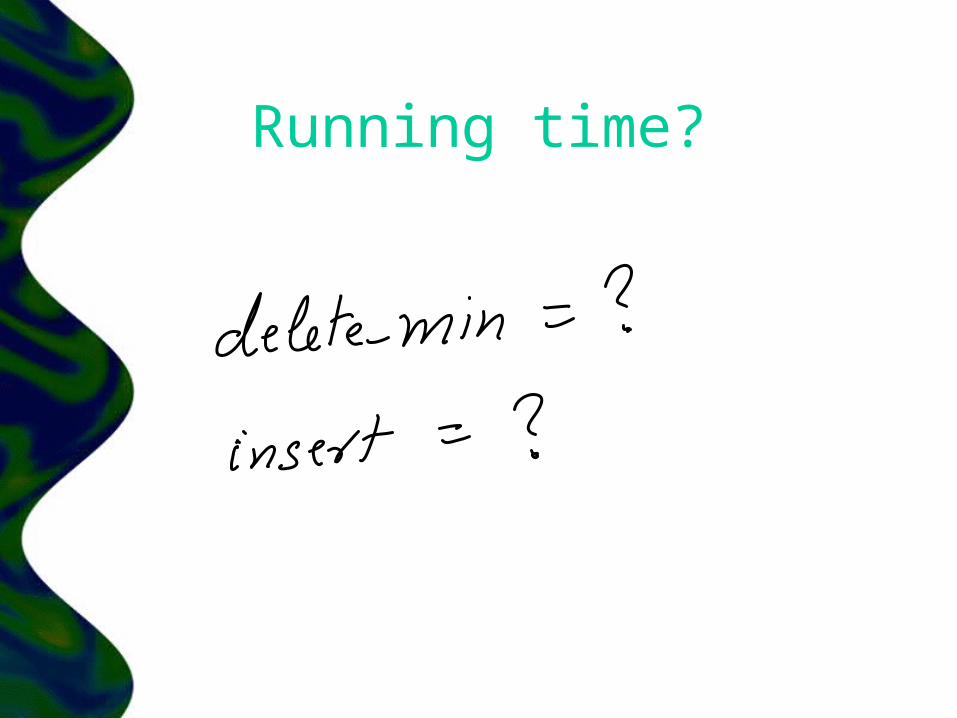
Running time?

Running time?

Running time?
• If we used a linked list as our magic data structure?
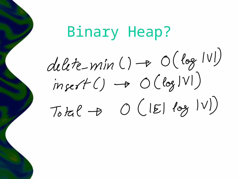
Binary Heap?

d-ary heap

Fibonacci Heap
a Spanning tree
• Recall?• Is it unique?• Is shortest path tree a spanning
tree?• Is there an easy way to build a
spanning tree for a given graph G? • Is it defined for disconnected
graphs?

Spanning tree
Connected subset of a graph G with n-1 edges which contains all of V.
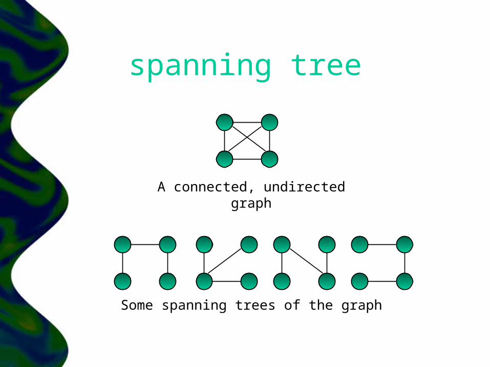
spanning tree
A connected, undirected graph
Some spanning trees of the graph
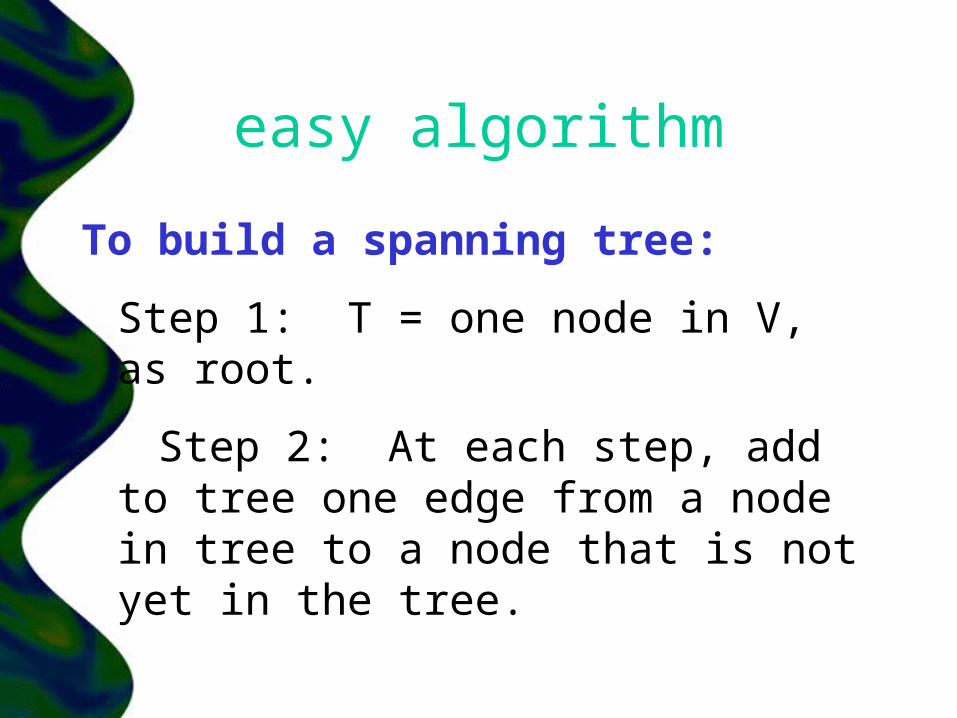
easy algorithm
To build a spanning tree:
Step 1: T = one node in V, as root.
Step 2: At each step, add to tree one edge from a node in tree to a node that is not yet in the tree.

Spanning tree property
Adding an edge e=(a,b) not in the tree creates a cycle containing only edge e and edges in spanning tree.
Why?
Spanning tree property
• Let c be the first node common to the path from a and b to the root of the spanning tree.
• The concatenation of (a,b) (b,c) (c,a) gives us the desired cycle.
lemma 1
• In any tree, T = (V,E), |E| = |V| - 1
• Why?
lemma 1
• In any tree, T = (V,E), |E| = |V| - 1
• Why?• Tree T with 1 node has zero edges.• For all n>0, P(n) holds, where• P(n) : A Tree with n nodes has n-1 edges.• Apply MI. How do we prove that given
P(m) true for all 1..m, P(m+1) is true?

undirected graphs n trees
• An undirected graph G = (V,E) is a tree iff (1) it is connected
(2) |E| = |V| – 1

Lemma 2
Let C be the cycle created in a spanning tree T by adding the edge e = (a,b) not in the tree. Then removing any edge from C yields another spanning tree.
Why? How many edges and vertices does the new graph have? Can (x,y) in G get disconnected in this new tree?

LEMMA 2
• Let T’ be the new graph• T’ has n nodes and n-1 edges, so it must
be a tree if it is connected.• Let (x,y) be not connected in T’. The
only problem in the connection can be the removed edge (a,b). But if (a,b) was contained in the path from x to y, we can use the cycle C to reach y (even if (a,b) was deleted from the graph).

weighted spanning trees
Let we be the weight of an edge e in G=(V,E).
Weight of spanning tree = Sum of edge weights.
Question: How do we find the spanning tree with minimum weight.
This spanning tree is also called the Minimum Spanning Tree.
Is the MST unique?
minimum spanning trees
• Applications– networks– cluster analysis
• used in graphics/pattern recognition
– approximation algorithms (TSP)– bioinformatics/CFD

cut property
• Let X be a subset of V. Among edges crossing between X and V \ X, let e be the edge of minimum weight. Then e belongs to the MST.
• Proof?

cycle property
• For any cycle C in a graph, the heaviest edge in C does not appear in the MST.
• Proof?
double chocolate question
• Is the SSSP Tree and the Minimum spanning tree the same?
• Is one the subset of the other always?

double chocolate question
• Is the SSSP Tree and the Minimum spanning tree the same?
• Is one the subset of the other always?
4 4
1
4 4 4
1
SSSP Tree MST
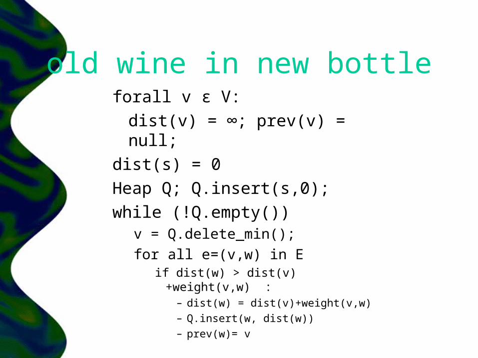
old wine in new bottleforall v ε V:
dist(v) = ∞; prev(v) = null;dist(s) = 0Heap Q; Q.insert(s,0);while (!Q.empty())
v = Q.delete_min();for all e=(v,w) in E
if dist(w) > dist(v)+weight(v,w) :
– dist(w) = dist(v)+weight(v,w)– Q.insert(w, dist(w))– prev(w)= v

a slight modificationjarnik’s or prim’s alg.
forall v ε V: dist(v) = ∞; prev(v) = null;
dist(s) = 0Heap Q; Q.insert(s,0);while (!Q.empty())
v = Q.delete_min();for all e=(v,w) in E
if dist(w) > dist(v)+ weight(v,w) :
– dist(w) = dist(v) + weight(v,w)– Q.insert(w, dist(w))– prev(w)= v

our first MST alg.forall v ε V:
dist(v) = ∞; prev(v) = null;
dist(s) = 0Magic_DS Q; Q.insert(s,0);while (!Q.empty())
v = Q.delete_min();for all e=(v,w) in E
if dist(w) > weight(v,w) : – dist(w) = weight(v,w)– Q.insert(w, dist(w))– prev(w)= v

how does the running time depend on the magic_Ds?
• heap?• insert()?• delete_min()?• Total time? • What if we change the Magic_DS to
fibonacci heap?

prim’s/jarnik’s algorithm
• best running time using fibonacci heaps– O(E + VlogV)
• Why does it compute the MST?

another alg: KRushkal’s
• sort the edges of G in increasing order of weights
• Let S = {}• for each edge e in G in sorted
order– if the endpoints of e are disconnected
in S– Add e to S
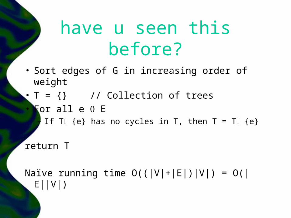
have u seen this before?
• Sort edges of G in increasing order of weight
• T = {} // Collection of trees• For all e E
– If T {e} has no cycles in T, then T = T {e}
return T
Naïve running time O((|V|+|E|)|V|) = O(|E||V|)

how to speed it up?
• To O(E + VlogV)– Note that this is achieved by fibonacci
heaps.
• Surprisingly the idea is very simple.