gnuplot Quick Reference(Copyright(c) Alex Woo 1992 June 1)

Updated by Hans-Bernhard Broker, April 2004

Starting gnuplot

to enter gnuplot gnuplot

to enter batch gnuplot gnuplot macro_file

to pipe commands to gnuplot application | gnuplot

see below for environment variables you might want to change before entering gnuplot.

Exiting gnuplot

exit gnuplot quit

All gnuplot commands can be abbreviated to the first few unique letters, usually three characters.This reference uses the complete name for clarity.

Getting Help

introductory help help plot

help on a topic help <topic>

list of all help available help or ?

show current environment show all

Command-line Editing

The UNIX, MS-DOS and VMS versions of gnuplot support command-line editing and a commandhistory. EMACS style editing is supported.

Line Editing:

move back a single character ^ B

move forward a single character ^ F

moves to the beginning of the line ^ A

moves to the end of the line ^ E

delete the previous character ^ H and DEL

deletes the current character ^ D

deletes to the end of line ^ K

redraws line in case it gets trashed ^ L,^ R

deletes the entire line ^ U

deletes the last word ^ W

History:

moves back through history ^ P

moves forward through history ^ N

The following arrow keys may be used on most PC versions if READLINE is used.

IBM PC Arrow Keys:

Left Arrow same as ^ B

Right Arrow same as ^ F

Ctrl Left Arrow same as ^ A

Ctrl Right Arrow same as ^ E

Up Arrow same as ^ P

Down Arrow same as ^ N

Graphics Devices

All screen graphics devices are specified by names and options. This information can be read froma startup file (.gnuplot in UNIX). If you change the graphics device, you must replot with thereplot command or recreate it repeating the load of the script that created it.

get a list of valid devices set terminal [options]

Graphics Terminals:

Mac OS X set term aqua

AED 512 Terminal set term aed512

AED 767 Terminal set term aed767

Amiga set term amiga

Adobe Illustrator 3.0 Format set term aifm

Apollo graphics primitive, rescalable set term apollo

Atari ST set term atari

BBN Bitgraph Terminal set term bitgraph

SCO CGI Driver set term cgi

Apollo graphics primitive, fixed window set term gpr

SGI GL window set term iris4d [8 24]

MS-DOS Kermit Tek4010 term - color set term kc_tek40xx

MS-DOS Kermit Tek4010 term - mono set term km_tek40xx

NeXTstep window system set term next

OS/2 Presentation Manager set term pm

REGIS graphics language set term regis

Selanar Tek Terminal set term selanar

SunView window system set term sun

Tektronix 4106, 4107, 4109 & 420X set term tek4OD10x

Tektronix 4010; most TEK emulators set term tek40xx

VAX UIS window system set term VMS

VT-like tek40xx terminal emulator set term vttek

UNIX plotting (not always supplied) set term unixplot

AT&T 3b1 or 7300 UNIXPC set term unixpc

MS Windows set term windows

X11 display terminal set term x11

Turbo C PC Graphics Modes:

Hercules set term hercules

Color Graphics Adaptor set term cga

Monochrome CGA set term mcga

Extended Graphics Adaptor set term ega

VGA set term vga

Monochrome VGA set term vgamono

Super VGA - requires SVGA driver set term svga

AT&T 6300 Micro set term att

Hardcopy Devices:

Unknown - not a plotting device set term unknown

Dump ASCII table of X Y [Z] values set term table

printer or glass dumb terminal set term dumb

Roland DXY800A plotter set term dxy800a

Dot Matrix Printers

Epson-style 60-dot per inch printers set term epson_60dpi

Epson LX-800, Star NL-10 set term epson_lx800

NX-1000, PROPRINTER set term epson_lx800

NEC printer CP6, Epson LQ-800 set term nec_cp6 [monochrome color draft]

Star Color Printer set term starc

Tandy DMP-130 60-dot per inch set term tandy_60dpi

Vectrix 384 & Tandy color printer set term vx384

Laser Printers

1

Talaris EXCL language set term excl

Imagen laser printer set term imagen

LN03-Plus in EGM mode set term ln03

PostScript graphics language set term post [mode color ‘font’ size]

CorelDraw EPS set term corel [mode color ‘font’ size]

Prescribe - for the Kyocera Laser Printer set term prescribe

Kyocera Laser Printer with Courier font set term kyo

QMS/QUIC Laser (also Talaris 1200 ) set term qms

Metafiles

AutoCAD DXF (120x80 default) set term dxf

FIG graphics language: SunView or X set term fig

FIG graphics language: Large Graph set term bfig

SCO hardcopy CGI set term hcgi

Frame Maker MIF 3.0 set term mif [pentype curvetype help]

Portable bitmap set term pbm [fontsize color]

Uniplex Redwood Graphics Interface Proto-col

set term rgip

TGIF language set term tgif

HP Devices

HP2623A and maybe others set term hp2623A

HP2648 and HP2647 set term hp2648

HP7580, & probably other HPs (4 pens) set term hp7580B

HP7475 & lots of others (6 pens) set term hpgl

HP Laserjet series II & clones set term hpljii [75 100 150 300]

HP DeskJet 500 set term hpdj [75 100 150 300]

HP PaintJet & HP3630 set term hppj [FNT5X9 FNT9X17 FNT13x25]

HP laserjet III ( HPGL plot vectors) set term pcl5 [mode font fontsize ]

TeX picture environments

LaTeX picture environment set term latex

EEPIC – extended LaTeX picture set term eepic

LaTeX picture with emTeX specials set term emtex

PSTricks macros for TeX or LaTeX set term pstricks

TPIC specials for TeX or LaTeX set term tpic

MetaFont font generation input set term mf

Saving and restoring terminal

restore default or pushed terminal set term pop

save (push) current terminal set term push

Commands associated to interactive terminals

change mouse settings set mouse

change hotkey bindings bind

Files

plot a data file plot ‘fspec’

load in a macro file load ‘fspec’

save command buffer to a macro file save ‘fspec’

save settings for later reuse save set ‘fpec’

PLOT & SPLOT commands

plot and splot are the primary commands plot is used to plot 2-d functions and data, whilesplot plots 3-d surfaces and data.

Syntax:

plot {ranges} <function> {title}{style} {,<function> {title}{style}...}splot {ranges} <function> {title}{style} {,<function> {title}{style}...}where <function> is either a mathematical expression, the name of a data file enclosed in quotes,or a pair (plot) or triple (splot) of mathematical expressions in the case of parametric functions.User-defined functions and variables may also be defined here. Examples will be given below.

Plotting Data

Discrete data contained in a file can displayed by specifying the name of the data file (enclosedin quotes) on the plot or splot command line. Data files should contain one data point per line.Lines beginning with # (or ! on VMS) will be treated as comments and ignored. For plots,each data point represents an (x,y) pair. For splots, each point is an (x,y,z) triple. For plotswith error bars (see plot errorbars), each data point is either (x,y,ydelta), (x,y,ylow,yhigh),(x,y,xlow,xhigh), (x,y,xdelta,ydelta), or (x,y,xlow,xhigh,ylow,yhigh). In all cases, the numbers oneach line of a data file must be separated by blank space. This blank space divides each line intocolumns.

For plots the x value may be omitted, and for splots the x and y values may be omitted. Ineither case the omitted values are assigned the current coordinate number. Coordinate numbersstart at 0 and are incremented for each data point read.

Surface Plotting

Implicitly, there are two types of 3-d datafiles. If all the isolines are of the same length, the data isassumed to be a grid data, i.e., the data has a grid topology. Cross isolines in the other parametricdirection (the ith cross isoline passes thru the ith point of all the provided isolines) will also bedrawn for grid data. (Note contouring is available for grid data only.) If all the isolines are not ofthe same length, no cross isolines will be drawn and contouring that data is impossible.

Using Pipes

On some computer systems with a popen function (Unix, plus some others), the datafile can bepiped through a shell command by starting the file name with a ’<’. For example:

pop(x) = 103*exp(x/10) plot ”< awk ’{ print $1-1965 $2 }’ population.dat”, pop(x)

would plot the same information as the first population example but with years since 1965 as thex axis. Simple manipulations of this kind can also be done using the extended capabilties of using

Similarly, output can be piped to another application, e.g.

set out ”|lpr -Pmy laser printer”

2

Plot Data Using

The format of data within a file can be selected with the using option. An explicit scanf stringcan be used, or simpler column choices can be made.

plot ”datafile” { using {<ycol> |<xcol>:<ycol> |<xcol>:<ycol>:<ydelta> |<xcol>:<ycol>:<width> |<xcol>:<ycol>:<xdelta> |<xcol>:<ycol>:<ylo>:<yhi> |<xcol>:<ycol>:<xlo>:<xhi> |<xcol>:<ycol>:<xdelta>:<ydelta> |<xcol>:<ycol>:<ydelta>:<width> |<xcol>:<ycol>:<ylo>:<yhi>:<width> |<xc>:<yc>:<xlo>:<xhi>:<ylo>:<yhi>}{"<scanf string>"}}...

splot ”datafile” { using {<xcol>:<ycol>:<zcol>}{” <scanf string> ”}}...

<xcol>, <ycol>, and <zcol> explicitly select the columns to plot from a space or tab separatedmulticolumn data file. If only <ycol> is selected for plot, <xcol> defaults to 1. If only <zcol>is selected for splot, then only that column is read from the file. An <xcol> of 0 forces <ycol>to be plotted versus its coordinate number. <xcol>, <ycol>, and <zcol> can be entered asconstants or expressions. Expressions enclosed in parentheses can be used to compute a columndata value from all numbers in the input record.

If errorbars (see also plot errorbars) are used for plots, xdelta or ydelta (for example, a +/-error) should be provided as the third column, or (x,y)low and (x,y)high as third and fourthcolumns. These columns must follow the x and y columns. If errorbars in both directions arewanted then xdelta and ydelta should be in the third and fourth columns, respectively, or xlow,xhigh, ylow, yhigh should be in the third, fourth, fifth, and sixth columns, respectively.

Scanf strings override any <xcol>:<ycol>(:<zcol>) choices, except for ordering of input, e.g.,

plot ”datafile” using 2:1 "%f%*f%f"

causes the first column to be y and the third column to be x.

If the scanf string is omitted, the default is generated based on the <xcol>:<ycol>(:<zcol>)choices. If the using option is omitted, ”%f%f” is used for plot (”%f%f%f%f” or ”%f%f%f%f%f%f”for errorbar plots) and ”%f%f%f” is used for splot.

plot ”MyData” using "%*f%f%*20[^\n]%f" w lines

Data are read from the file “MyData” using the format ”%*f%f%*20[ˆ\n]%f”. The meaning ofthis format is: ”%*f” ignore the first number, ”%f” then read in the second and assign to x,”%*20[ˆ\n]” then ignore 20 non-newline characters, ”%f” then read in the y value.

Plot With Errorbars

Error bars are supported for 2-d data file plots by reading one to four additional columns specifyingydelta, ylow and yhigh, xdelta, xlow and xhigh, xdelta and ydelta, or xlow, xhigh, ylow, and yhighrespectively. No support exists for error bars for splots.

In the default situation, gnuplot expects to see three to six numbers on each line of the data file,either (x, y, ydelta), (x, y, ylow, yhigh), (x, y, xdelta), (x, y, xlow, xhigh), (x, y, xdelta, ydelta),or (x, y, xlow, xhigh, ylow, yhigh). The x coordinate must be specified. The order of the numbersmust be exactly as given above. Data files in this format can easily be plotted with error bars:

plot ”data.dat” with errorbars (or yerrorbars)

plot ”data.dat” with xerrorbars

plot ”data.dat” with xyerrorbars

The error bar is a line plotted from (x, ylow) to (x, yhigh) or (xlow, y) to (xhigh, y). If ydelta isspecified instead of ylow and yhigh, ylow=y-ydelta and yhigh=y+ydelta are derived. The valuesfor xlow and xhigh are derived similarly from xdelta. If there are only two numbers on the line,yhigh and ylow are both set to y and xhigh and xlow are both set to x. To get lines plottedbetween the data points, plot the data file twice, once with errorbars and once with lines.

If x or y autoscaling is on, the x or y range will be adjusted to fit the error bars.

Boxes may be drawn with y error bars using the boxerrorbars style. The width of the box maybe either set with the ”set boxwidth” command, given in one of the data columns, or calculatedautomatically so each box touches the adjacent boxes. Boxes may be drawn instead of the crossdrawn for the xyerrorbars style by using the boxxyerrorbars style.

x,y,ylow & yhigh from columns 1,2,3,4 plot "data.dat" us 1:2:3:4 w errorbars

x from third, y from second, xdelta from 6 plot "data.dat" using 3:2:6 w xerrorbars

x,y,xdelta & ydelta from columns 1,2,3,4 plot "data.dat" us 1:2:3:4 w xyerrorbars

Plot Ranges

The optional range specifies the region of the plot that will be displayed.

Ranges may be provided on the plot and splot command line and affect only that plot, or in theset xrange, set yrange, etc., commands, to change the default ranges for future plots.

[{<dummy-var>=}{<xmin>:<xmax>}] { [{<ymin>:<ymax>}] }where <dummy-var> is the independent variable (the defaults are x and y, but this may bechanged with set dummy) and the min and max terms can be constant expressions.

Both the min and max terms are optional. The ’:’ is also optional if neither a min nor a max termis specified. This allows ’[ ]’ to be used as a null range specification.

Specifying a range in the plot command line turns autoscaling for that axis off for that plot. Usingone of the set range commands turns autoscaling off for that axis for future plots, unless changedlater. (See set autoscale).

This uses the current ranges plot cos(x)

This sets the x range only plot [-10:30] sin(pi*x)/(pi*x)

This sets both the x and y ranges plot [-pi:pi] [-3:3] tan(x), 1/x

sets only y range, & plot [ ] [-2:sin(5)*-8] sin(x)**besj0(x)

turns off autoscaling on both axesThis sets xmax and ymin only plot [:200] [-pi:] exp(sin(x))

This sets the x, y, and z ranges splot [0:3] [1:4] [-1:1] x*y

3

Plot With Style

Plots may be displayed in one of twelve styles: lines, points, linespoints, impulses, dots, steps,errorbars (or yerrorbars), xerrorbars, xyerrorbars, boxes, boxerrorbars, or boxxyerror-

bars. The lines style connects adjacent points with lines. The points style displays a smallsymbol at each point. The linespoints style does both lines and points. The impulses styledisplays a vertical line from the x axis (or from the grid base for splot) to each point. The dots

style plots a tiny dot at each point; this is useful for scatter plots with many points. The steps

style is used for drawing stairstep-like functions. The boxes style may be used for barcharts.

The errorbars style is only relevant to 2-d data file plotting. It is treated like points for splotsand function plots. For data plots, errorbars is like points, except that a vertical error bar isalso drawn: for each point (x,y), a line is drawn from (x,ylow) to (x,yhigh). A tic mark is placedat the ends of the error bar. The ylow and yhigh values are read from the data file’s columns, asspecified with the using option to plot. The xerrorbars style is similar except that it draws ahorizontal error bar from xlow to xhigh. The xyerrorbars or boxxyerrorbars style is used fordata with errors in both x and y. A barchart style may be used in conjunction with y error barsthrough the use of boxerrorbars. The See plot errorbars for more information.

Default styles are chosen with the set function style and set data style commands.

By default, each function and data file will use a different line type and point type, up to themaximum number of available types. All terminal drivers support at least six different pointtypes, and re-use them, in order, if more than six are required. The LaTeX driver supplies anadditional six point types (all variants of a circle), and thus will only repeat after twelve curvesare plotted with points.

If desired, the style and (optionally) the line type and point type used for a curve can be specified.

with <style> {<linetype> {<pointtype>}}where <style> is either lines, points, linespoints, impulses, dots, steps, errorbars (oryerrorbars), xerrorbars, xyerrorbars, boxes, boxerrorbars, boxxyerrorbars.

The <linetype> & <pointtype> are positive integer constants or expressions and specify the linetype and point type to be used for the plot. Line type 1 is the first line type used by default, linetype 2 is the second line type used by default, etc.

plots sin(x) with impulses plot sin(x) with impulses

plots x*y with points, x**2 + y**2 default splot x*y w points, x**2 + y**2

plots tan(x) with default function style plot [ ] [-2:5] tan(x)

plots “data.1” with lines plot "data.1" with l

plots “leastsq.dat” with impulses plot ’leastsq.dat’ w i

plots “exper.dat” with errorbars & plot ’exper.dat’ w l, ’exper.dat’ w err

lines connecting points

Here ’exper.dat’ should have three or four data columns.

plots x**2 + y**2 and x**2 - y**2 with thesame line type

splot x**2 + y**2 w l 1, x**2 - y**2 w l 1

plots sin(x) and cos(x) with linespoints, using plot sin(x) w linesp 1 3, \

the same line type but different point types cos(x) w linesp 1 4

plots file “data” with points style 3 plot "data" with points 1 3

Note that the line style must be specified when specifying the point style, even when it is irrelevant.Here the line style is 1 and the point style is 3, and the line style is irrelevant.

See set style to change the default styles.

Plot Title

A title of each plot appears in the key. By default the title is the function or file name as it appearson the plot command line. The title can be changed by using the title option. This option shouldprecede any with option.

title ”<title>”

where <title> is the new title of the plot and must be enclosed in quotes. The quotes will not beshown in the key.

plots y=x with the title ’x’ plot x

plots the “glass.dat” file splot "glass.dat" tit ’revolution surface’

with the title ’revolution surface’plots x squared with title “xˆ2” and “data.1” plot x**2 t "x^2", \

with title ’measured data’ "data.1" t ’measured data’

4

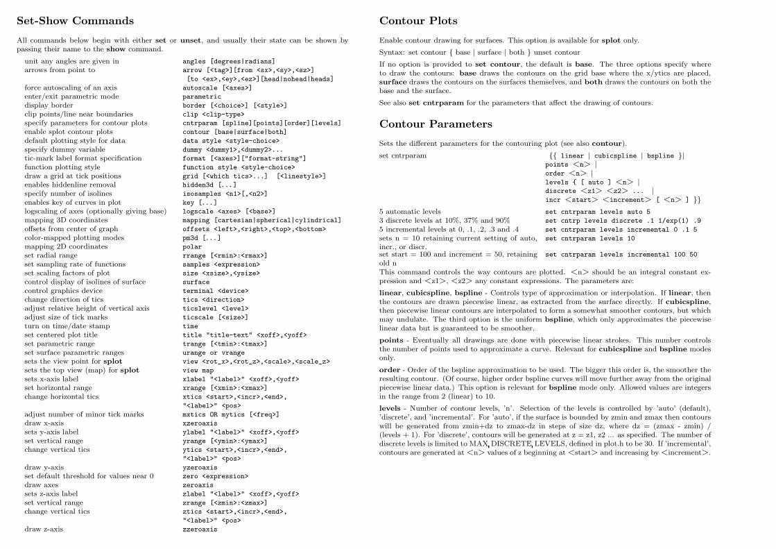
Set-Show Commands

All commands below begin with either set or unset, and usually their state can be shown bypassing their name to the show command.

unit any angles are given in angles [degrees|radians]

arrows from point to arrow [<tag>][from <sx>,<sy>,<sz>]

[to <ex>,<ey>,<ez>][head|nohead|heads]

force autoscaling of an axis autoscale [<axes>]

enter/exit parametric mode parametric

display border border [<choice>] [<style>]

clip points/line near boundaries clip <clip-type>

specify parameters for contour plots cntrparam [spline][points][order][levels]

enable splot contour plots contour [base|surface|both]

default plotting style for data data style <style-choice>

specify dummy variable dummy <dummy1>,<dummy2>...

tic-mark label format specification format [<axes>]["format-string"]

function plotting style function style <style-choice>

draw a grid at tick positions grid [<which tics>...] [<linestyle>]

enables hiddenline removal hidden3d [. . . ]specify number of isolines isosamples <n1>[,<n2>]

enables key of curves in plot key [. . . ]logscaling of axes (optionally giving base) logscale <axes> [<base>]

mapping 3D coordinates mapping [cartesian|spherical|cylindrical]

offsets from center of graph offsets <left>,<right>,<top>,<bottom>

color-mapped plotting modes pm3d [. . . ]mapping 2D coordinates polar

set radial range rrange [<rmin>:<rmax>]

set sampling rate of functions samples <expression>

set scaling factors of plot size <xsize>,<ysize>

control display of isolines of surface surface

control graphics device terminal <device>

change direction of tics tics <direction>

adjust relative height of vertical axis ticslevel <level>

adjust size of tick marks ticscale [<size>]

turn on time/date stamp time

set centered plot title title "title-text" <xoff>,<yoff>

set parametric range trange [<tmin>:<tmax>]

set surface parametric ranges urange or vrange

sets the view point for splot view <rot_x>,<rot_z>,<scale>,<scale_z>

sets the top view (map) for splot view map

sets x-axis label xlabel "<label>" <xoff>,<yoff>

set horizontal range xrange [<xmin>:<xmax>]

change horizontal tics xtics <start>,<incr>,<end>,

"<label>" <pos>

adjust number of minor tick marks mxtics OR mytics [<freq>]

draw x-axis xzeroaxis

sets y-axis label ylabel "<label>" <xoff>,<yoff>

set vertical range yrange [<ymin>:<ymax>]

change vertical tics ytics <start>,<incr>,<end>,

"<label>" <pos>

draw y-axis yzeroaxis

set default threshold for values near 0 zero <expression>

draw axes zeroaxis

sets z-axis label zlabel "<label>" <xoff>,<yoff>

set vertical range zrange [<zmin>:<zmax>]

change vertical tics ztics <start>,<incr>,<end>,

"<label>" <pos>

draw z-axis zzeroaxis

Contour Plots

Enable contour drawing for surfaces. This option is available for splot only.

Syntax: set contour { base | surface | both } unset contour

If no option is provided to set contour, the default is base. The three options specify whereto draw the contours: base draws the contours on the grid base where the x/ytics are placed,surface draws the contours on the surfaces themselves, and both draws the contours on both thebase and the surface.

See also set cntrparam for the parameters that affect the drawing of contours.

Contour Parameters

Sets the different parameters for the contouring plot (see also contour).

set cntrparam {{ linear | cubicspline | bspline }|points <n> |order <n> |levels { [ auto ] <n> |discrete <z1> <z2> ... |incr <start> <increment> [ <n> ] }}

5 automatic levels set cntrparam levels auto 5

3 discrete levels at 10%, 37% and 90% set cntrp levels discrete .1 1/exp(1) .9

5 incremental levels at 0, .1, .2, .3 and .4 set cntrparam levels incremental 0 .1 5

sets n = 10 retaining current setting of auto,incr., or discr.

set cntrparam levels 10

set start = 100 and increment = 50, retainingold n

set cntrparam levels incremental 100 50

This command controls the way contours are plotted. <n> should be an integral constant ex-pression and <z1>, <z2> any constant expressions. The parameters are:

linear, cubicspline, bspline - Controls type of approximation or interpolation. If linear, thenthe contours are drawn piecewise linear, as extracted from the surface directly. If cubicspline,then piecewise linear contours are interpolated to form a somewhat smoother contours, but whichmay undulate. The third option is the uniform bspline, which only approximates the piecewiselinear data but is guaranteed to be smoother.

points - Eventually all drawings are done with piecewise linear strokes. This number controlsthe number of points used to approximate a curve. Relevant for cubicspline and bspline modesonly.

order - Order of the bspline approximation to be used. The bigger this order is, the smoother theresulting contour. (Of course, higher order bspline curves will move further away from the originalpiecewise linear data.) This option is relevant for bspline mode only. Allowed values are integersin the range from 2 (linear) to 10.

levels - Number of contour levels, ’n’. Selection of the levels is controlled by ’auto’ (default),’discrete’, and ’incremental’. For ’auto’, if the surface is bounded by zmin and zmax then contourswill be generated from zmin+dz to zmax-dz in steps of size dz, where dz = (zmax - zmin) /(levels + 1). For ’discrete’, contours will be generated at z = z1, z2 ... as specified. The number ofdiscrete levels is limited to MAX DISCRETE LEVELS, defined in plot.h to be 30. If ’incremental’,contours are generated at <n> values of z beginning at <start> and increasing by <increment>.

5

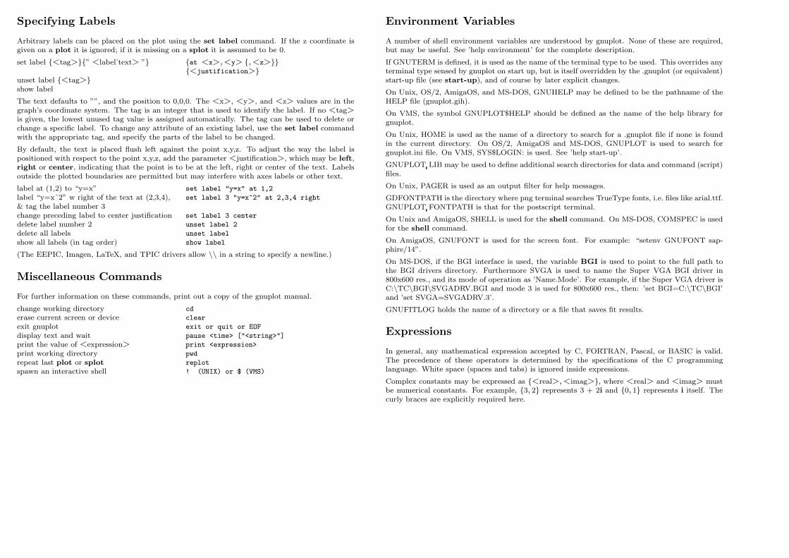
Specifying Labels

Arbitrary labels can be placed on the plot using the set label command. If the z coordinate isgiven on a plot it is ignored; if it is missing on a splot it is assumed to be 0.

set label {<tag>}{” <label˙text> ”} {at <x>,<y> {,<z>}}{<justification>}

unset label {<tag>}show label

The text defaults to ””, and the position to 0,0,0. The <x>, <y>, and <z> values are in thegraph’s coordinate system. The tag is an integer that is used to identify the label. If no <tag>is given, the lowest unused tag value is assigned automatically. The tag can be used to delete orchange a specific label. To change any attribute of an existing label, use the set label commandwith the appropriate tag, and specify the parts of the label to be changed.

By default, the text is placed flush left against the point x,y,z. To adjust the way the label ispositioned with respect to the point x,y,z, add the parameter <justification>, which may be left,right or center, indicating that the point is to be at the left, right or center of the text. Labelsoutside the plotted boundaries are permitted but may interfere with axes labels or other text.

label at (1,2) to “y=x” set label "y=x" at 1,2

label “y=xˆ2” w right of the text at (2,3,4), set label 3 "y=x^2" at 2,3,4 right

& tag the label number 3change preceding label to center justification set label 3 center

delete label number 2 unset label 2

delete all labels unset label

show all labels (in tag order) show label

(The EEPIC, Imagen, LaTeX, and TPIC drivers allow \\ in a string to specify a newline.)

Miscellaneous Commands

For further information on these commands, print out a copy of the gnuplot manual.

change working directory cd

erase current screen or device clear

exit gnuplot exit or quit or EOF

display text and wait pause <time> ["<string>"]

print the value of <expression> print <expression>

print working directory pwd

repeat last plot or splot replot

spawn an interactive shell ! (UNIX) or $ (VMS)

Environment Variables

A number of shell environment variables are understood by gnuplot. None of these are required,but may be useful. See ’help environment’ for the complete description.

If GNUTERM is defined, it is used as the name of the terminal type to be used. This overrides anyterminal type sensed by gnuplot on start up, but is itself overridden by the .gnuplot (or equivalent)start-up file (see start-up), and of course by later explicit changes.

On Unix, OS/2, AmigaOS, and MS-DOS, GNUHELP may be defined to be the pathname of theHELP file (gnuplot.gih).

On VMS, the symbol GNUPLOT$HELP should be defined as the name of the help library forgnuplot.

On Unix, HOME is used as the name of a directory to search for a .gnuplot file if none is foundin the current directory. On OS/2, AmigaOS and MS-DOS, GNUPLOT is used to search forgnuplot.ini file. On VMS, SYS$LOGIN: is used. See ’help start-up’.

GNUPLOT LIB may be used to define additional search directories for data and command (script)files.

On Unix, PAGER is used as an output filter for help messages.

GDFONTPATH is the directory where png terminal searches TrueType fonts, i.e. files like arial.ttf.GNUPLOT FONTPATH is that for the postscript terminal.

On Unix and AmigaOS, SHELL is used for the shell command. On MS-DOS, COMSPEC is usedfor the shell command.

On AmigaOS, GNUFONT is used for the screen font. For example: “setenv GNUFONT sap-phire/14”.

On MS-DOS, if the BGI interface is used, the variable BGI is used to point to the full path tothe BGI drivers directory. Furthermore SVGA is used to name the Super VGA BGI driver in800x600 res., and its mode of operation as ’Name.Mode’. For example, if the Super VGA driver isC:\TC\BGI\SVGADRV.BGI and mode 3 is used for 800x600 res., then: ’set BGI=C:\TC\BGI’and ’set SVGA=SVGADRV.3’.

GNUFITLOG holds the name of a directory or a file that saves fit results.

Expressions

In general, any mathematical expression accepted by C, FORTRAN, Pascal, or BASIC is valid.The precedence of these operators is determined by the specifications of the C programminglanguage. White space (spaces and tabs) is ignored inside expressions.

Complex constants may be expressed as {<real>,<imag>}, where <real> and <imag> mustbe numerical constants. For example, {3, 2} represents 3 + 2i and {0, 1} represents i itself. Thecurly braces are explicitly required here.

6

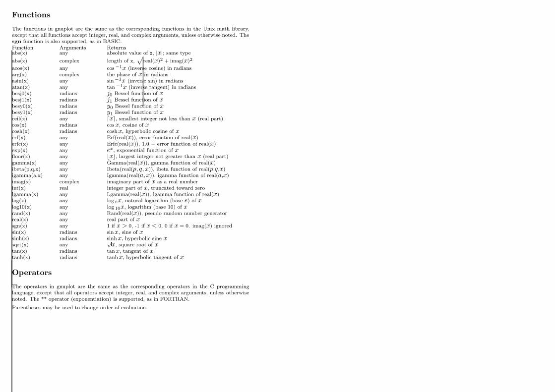
Functions

The functions in gnuplot are the same as the corresponding functions in the Unix math library,except that all functions accept integer, real, and complex arguments, unless otherwise noted. Thesgn function is also supported, as in BASIC.Function Arguments Returnsabs(x) any absolute value of x, |x|; same type

abs(x) complex length of x,√

real(x)2 + imag(x)2

acos(x) any cos−1x (inverse cosine) in radiansarg(x) complex the phase of x in radiansasin(x) any sin−1x (inverse sin) in radiansatan(x) any tan −1x (inverse tangent) in radiansbesj0(x) radians j0 Bessel function of xbesj1(x) radians j1 Bessel function of xbesy0(x) radians y0 Bessel function of xbesy1(x) radians y1 Bessel function of xceil(x) any dxe, smallest integer not less than x (real part)cos(x) radians cosx, cosine of xcosh(x) radians coshx, hyperbolic cosine of xerf(x) any Erf(real(x)), error function of real(x)erfc(x) any Erfc(real(x)), 1.0 − error function of real(x)exp(x) any ex, exponential function of xfloor(x) any bxc, largest integer not greater than x (real part)gamma(x) any Gamma(real(x)), gamma function of real(x)ibeta(p,q,x) any Ibeta(real(p, q, x)), ibeta function of real(p,q,x)igamma(a,x) any Igamma(real(a,x)), igamma function of real(a,x)imag(x) complex imaginary part of x as a real numberint(x) real integer part of x, truncated toward zerolgamma(x) any Lgamma(real(x)), lgamma function of real(x)log(x) any log ex, natural logarithm (base e) of xlog10(x) any log 10x, logarithm (base 10) of xrand(x) any Rand(real(x)), pseudo random number generatorreal(x) any real part of xsgn(x) any 1 if x > 0, -1 if x < 0, 0 if x = 0. imag(x) ignoredsin(x) radians sinx, sine of xsinh(x) radians sinhx, hyperbolic sine xsqrt(x) any

√x, square root of x

tan(x) radians tan x, tangent of xtanh(x) radians tanh x, hyperbolic tangent of x

Operators

The operators in gnuplot are the same as the corresponding operators in the C programminglanguage, except that all operators accept integer, real, and complex arguments, unless otherwisenoted. The ** operator (exponentiation) is supported, as in FORTRAN.

Parentheses may be used to change order of evaluation.

7