graphical pilot interface simulator (gpis)

Louisiana State UniversityLSU Digital Commons

LSU Master's Theses Graduate School

2005

Graphical Pilot Interface Simulator (GPIS)Jeffry Jorge HandalLouisiana State University and Agricultural and Mechanical College, [email protected]

Follow this and additional works at: https://digitalcommons.lsu.edu/gradschool_theses

Part of the Electrical and Computer Engineering Commons

This Thesis is brought to you for free and open access by the Graduate School at LSU Digital Commons. It has been accepted for inclusion in LSUMaster's Theses by an authorized graduate school editor of LSU Digital Commons. For more information, please contact [email protected].

Recommended CitationHandal, Jeffry Jorge, "Graphical Pilot Interface Simulator (GPIS)" (2005). LSU Master's Theses. 3301.https://digitalcommons.lsu.edu/gradschool_theses/3301

https://digitalcommons.lsu.edu?utm_source=digitalcommons.lsu.edu%2Fgradschool_theses%2F3301&utm_medium=PDF&utm_campaign=PDFCoverPages

https://digitalcommons.lsu.edu/gradschool_theses?utm_source=digitalcommons.lsu.edu%2Fgradschool_theses%2F3301&utm_medium=PDF&utm_campaign=PDFCoverPages

https://digitalcommons.lsu.edu/gradschool?utm_source=digitalcommons.lsu.edu%2Fgradschool_theses%2F3301&utm_medium=PDF&utm_campaign=PDFCoverPages

https://digitalcommons.lsu.edu/gradschool_theses?utm_source=digitalcommons.lsu.edu%2Fgradschool_theses%2F3301&utm_medium=PDF&utm_campaign=PDFCoverPages

http://network.bepress.com/hgg/discipline/266?utm_source=digitalcommons.lsu.edu%2Fgradschool_theses%2F3301&utm_medium=PDF&utm_campaign=PDFCoverPages

https://digitalcommons.lsu.edu/gradschool_theses/3301?utm_source=digitalcommons.lsu.edu%2Fgradschool_theses%2F3301&utm_medium=PDF&utm_campaign=PDFCoverPages

mailto:[email protected]

GRAPHICAL PILOT INTERFACE SIMULATOR

(GPIS)

A Thesis

Submitted to the Graduate Faculty of the

Louisiana State University and Agricultural and Mechanical College

in partial fulfillment of the requirements for the degree of

Master of Science in Electrical Engineering

in

The Department of Electrical and Computer Engineering

by Jeffry Jorge Handal

B.S.E.E., Louisiana State University, 2003 December 2005

Dedication I want this project to mark the first step of the rest of my life. It is a new starting point for my professional and educational career that will open many doors to future success. The efforts put forth to completing this project are dedicated to God, my family, and my friends.

ii

Acknowledgements

First of all, I would like to thank God for giving me the energy, mental ability, courage,

and will to finish this thesis project for my Master’s Degree. Second, I would like to thank Dr. Jorge Aravena for his attentive direction and patient guidance. He deposited great faith in me to develop a tool that, honestly, I did not think could be completed. The task included skills in programming and controls knowledge that I did not posses. He took a gamble on me, but I responded positively with many late nights of hard work and some sleepless nights. Dr. Aravena thank you for helping me achieve my goals.

I am especially thankful for my fellow students in this project. On top of being available

to discuss my problems, they have been a constant source of encouragement and creative ideas. Lalitha Devarakonda, from India, helped me modify the Boeing 747 model and setup scripts. She was a patient guide while trying to help me understand the model. Also from India, Phalguna Rachinayani (Kumar), I thank you for the many hours of long discussions of airplane dynamics and controls.

My friends here in Baton Rouge, New Orleans, Honduras, and everywhere in the world

wherever they may be now, helped maintain my sanity during stressful times. Thanks to Pablo Suarez, Allan McNally, Juan Yip, Benjamin Medina, and Akram Mustafa for staying in touch, curious to find out what I was up to. My deepest gratitude to my roommate, Rigoberto Funes, and Gerardo Trejo for taking me out and keeping me up to date with the party scene; Katherine Nunez for her heart-felt warmth; Megan Bello for adopting a Honduran friend and checking my work; and everyone else, who, in one way or another, has influenced me in becoming a better person.

I would also like to include the Management at the Office of Telecommunications (OTC

Power!) at LSU for giving me the flexibility to attend class and work full time. I could not have made it to class without their consent that school is very important. My Managers and coworkers have played an important role in shaping both my professional and educational development.

Not all of life’s successes come without failure first. A person may not succeed until they

learn how to fail. A phrase I have picked up over the years clearly exemplifies my thoughts: “Why do we fall? So we can learn how to pick ourselves back up…” There were many times I was not able to get things to work as I intended them. Even everyday life’s events, such as having major surgery, which I painfully went through, and Hurricanes Katrina and Rita, can be enough to discourage anyone; however, I got up, regained courage, and continued to pursue my goals.

Finally, I want to thank my beloved parents. They have always stood behind me and my

brothers regardless of our decisions. They have rooted for me to get my degree and succeed in life more than anyone, including myself. And I cannot forget, my family, including my brothers Jorge, Javier, and Joshua who look up to me; my cousins Tania and Javier Chicas, who allowed me to retreat to their home on the weekends.

iii

Table of Contents Dedication....................................................................................................................................... ii Acknowledgements ....................................................................................................................... iii List of Tables................................................................................................................................. vi List of Figures ............................................................................................................................. vii Abstract ....................................................................................................................................... viii Chapter 1 Introduction ................................................................................................................................ 1

1.1 Overview............................................................................................................................... 1 1.1.1 Outline ........................................................................................................................... 1

1.2 Simulation and Visualization ................................................................................................ 2 1.2.1 Simulation...................................................................................................................... 2 1.2.2 Visualization and Animation ......................................................................................... 3 1.2.3 Reasons for a GUI ......................................................................................................... 4

1.3 Aircraft Safety....................................................................................................................... 4 2 Concepts of Aerodynamics ........................................................................................................ 6

2.1 Forces on an Airplane ........................................................................................................... 6 2.2 Aircraft Controls ................................................................................................................... 7 2.3 Basic Aerodynamics and Trimmed Flight ............................................................................ 8 2.4 The Test Aircraft ................................................................................................................... 8 2.5 The SIMULINK Model......................................................................................................... 9

3 MATLAB GUIs ........................................................................................................................ 10

3.1 Design Principles ................................................................................................................ 10 3.2 Design Process .................................................................................................................... 10 3.3 Graphic Object Hierarchy ................................................................................................... 11 3.4 UI Control Elements ........................................................................................................... 12 3.5 UI Control Properties .......................................................................................................... 12 3.6 Manipulating Properties ...................................................................................................... 13 3.7 The Handles Structure......................................................................................................... 13 3.8 Callbacks............................................................................................................................. 14 3.9 GUIDE ................................................................................................................................ 14 3.10 GPIS GUI Layout.............................................................................................................. 16

4 Animations in MATLAB ......................................................................................................... 19

4.1 Animation Capabilities in MATLAB.................................................................................. 19 4.2 Attitude Indicator ................................................................................................................ 20 4.3 Aircraft Display................................................................................................................... 21 4.4 Aircraft Animation .............................................................................................................. 21

4.4.1 Coordinate Rotation..................................................................................................... 21 4.4.2 Euler Angles ................................................................................................................ 22 4.4.3 Translation and Rotation.............................................................................................. 22

4.5 Stabilizer and Pedal Position Displays................................................................................ 23

iv

4.6 Interacting with SIMULINK............................................................................................... 23 4.6.1 S-Functions .................................................................................................................. 24 4.6.2 M-File S-Functions...................................................................................................... 24

5 Conclusion ................................................................................................................................. 25

5.1 Summary of Contributions.................................................................................................. 25 5.2 Limitations and Future Research ........................................................................................ 26

Bibliography................................................................................................................................. 28 Appendix A: GPIS Manual......................................................................................................... 32

A.1 User’s Manual .................................................................................................................... 32 A.2 Setting Up the Program...................................................................................................... 32 A.3 Program Initialization......................................................................................................... 33

A.3.1 Trimming the Aircraft................................................................................................. 34 A.4 Operation Modes................................................................................................................ 36

A.4.1 File Input Guidelines .................................................................................................. 36 A.5 Menu Bar............................................................................................................................ 37 A.6 Pushbuttons ........................................................................................................................ 37 A.7 Pilot Control Inputs ............................................................................................................ 38 A.8 Other Aids for User ............................................................................................................ 38 A.9 Feedback ............................................................................................................................ 39

Appendix B: Conventions ........................................................................................................... 40

B.1 Coordinate System for Attitude Indicator .......................................................................... 40 B.2 Rotation .............................................................................................................................. 40 B.3 Pilot Control Sign Convention ........................................................................................... 40

Appendix C: Implementation Tips ............................................................................................ 41 Appendix D: MATLAB Source Code ........................................................................................ 46 Appendix E: Boeing 747 Information ........................................................................................ 72

E.1 Cockpit Layout of Boeing 747 ........................................................................................... 72 E.2 Boeing 747 General Specs.................................................................................................. 73

Vita................................................................................................................................................ 75

v

List of Tables

3.1: UI control elements ................................................................................................................ 12 4.1: M-file S-function and corresponding callbacks based on flag value...................................... 24 A.1: Pilot keyboard actions ........................................................................................................... 38 E. 1: Boeing 747 performance and dimensions............................................................................. 73

vi

List of Figures 2.1 Basic forces that act on an airplane. .......................................................................................... 6 2.2 Aircraft Rotations: Body Axes .................................................................................................. 8 2.3 Picture of test aircraft, Boeing 747, which will be used in this project. .................................... 9 3.1 GUI design process ................................................................................................................. 11 3.2 Graphic object hierarchy built into the MATLAB programming environment ...................... 11 3.3 GUIDE environment ............................................................................................................... 15 3.4 Object Browser that allows visualizing of the relationships between components. ................ 16 3.5 Menu editor environment. ....................................................................................................... 16 3.6 SIMULINK model of Boeing 747-100/200 ............................................................................ 17 3.7 GPIS GUI ................................................................................................................................ 17 4.1 Attitude indicator..................................................................................................................... 20 4.2 Aircraft display on attitude indicator....................................................................................... 21 4.3 X-axis, Y-axis, and Z-axis rotation matrices........................................................................... 22 4.4 Stabilizer and rudder position displays, respectively .............................................................. 23 A.1 Weight and balance setup of airplane..................................................................................... 34 A.2 Configuration point and flight condition ................................................................................ 35 A.3 Trim conditions results ........................................................................................................... 35 A.4 Order of input values .............................................................................................................. 36 B.1 Coordinate system for rotations.............................................................................................. 40 C.1 Translation about the y-axis. ‘y’ corresponds to the pitch angle in degrees. .......................... 44 E.1 Pilot control inputs in a Boeing 747 cockpit ........................................................................... 72 E.2 General dimensions of the Boeing 747-400............................................................................ 73 E.3 General arrangement of the Boeing 747-400 .......................................................................... 74 E.4 Typical engine installed on a Boeing 747. Shown is cutaway JT9D engine (Pratt & Whitney).......................................................................................................................... 74

vii

Abstract The thesis develops a graphic interface for a dynamic system simulation implemented in

the SIMULINK environment. The dynamic system is a B747-200 modeled as a rigid body with six degrees of freedom. The equations and database of aerodynamic coefficients over the complete flight envelope were provided by NASA’s Langley Research Center for the research project “Aircraft Safety: Managing Control Upsets.” The purpose of the interface is to allow the user to “fly the plane from the keyboard;” i.e., interact with the simulation by manipulating, from the keyboard, the main control surfaces and engine thrust and observing the performance of the plane in a manner similar to the way a pilot sees it from the cockpit.

The Graphical Pilot Interface Simulator (GPIS) interface extends the capability of the

current simulator [2] and allows the collection of data under conditions that were not readily available before. Moreover, it permits the derivation of linear models around trajectories that are not necessarily steady state conditions, or trimming points.

Even though the work is focused to a particular model, the interface techniques

developed here are flexible and can be applied to other dynamic simulations. The value of visualization to help communicate results and get better understanding of a model’s behavior is greatly stressed.

viii

Chapter 1

Introduction

“Now we have already discussed imagination in the treatise On the Soul and we concluded there that thought is impossible without an image.” – Aristotle

As Aristotle noted many hundreds of years ago, visualization is the foundation for human

understanding [25]. With the advances in computer technology, scientific visualization has experienced tremendous growth, especially in the last couple of years. Scientists and engineers have developed computer programs and application software that simulate and model systems being studied. Through the use of graphics in simulation, more people, including the scientist and the engineer himself, can gain better understanding of the systems being modeled.

For this project, we have a fairly detailed simulation of a B747-200 that can we execute

but we cannot manipulate interactively. The model of the system, provided by NASA Langley Research Center [40], contains features that lend themselves to graphic definition. For example, the position of an aircraft control surface is more easily visualized than numerical examination of it. This example shows how a graphic user interface (GUI) can facilitate model understanding. Additionally, constructing a graphic model provides powerful feedback to the developer indicating him if the model is being built correctly. 1.1 Overview From the work of those in Delft University of Technology [1], to the efforts done by Andres Marcos at the University of Minnesota [2], we plan to take their work a step further to produce more realistic results for the engineering community. The research goal is to expand our test bed to more realistic, life-like inputs by analyzing flight in circumstances other than trimmed conditions. In other words, we are having the “plane flying on manual”. We aim to enhance our research and test concepts in situations that are not possible now.

The two main functional goals of this research project are interactive pilot simulation and animation generation. Interactive pilot simulation itself has two components: graphical user interface (GUI) design and code development. We present a realistic model for the flight simulation of a B747-200 using these processes. We take advantage of MATLAB's GUI-building and model-simulating environments to implement this interactive simulation. We also describe techniques that may allow this project to be extended to other fields where visualization is beneficial. 1.1.1 Outline This document is organized as follows: This chapter presents some background information necessary to understanding simulation and visualization and their role in this project. Additionally, we present a brief description on aircraft safety and the motivations it contributes to this research. Chapter 2 illustrates concepts in aerodynamics in order to give the user a working understanding of some of the technical vocabulary used in this field.

1

Chapter 3 summarizes GUI building procedures followed to develop the simulator tool. Many items in MATLAB that enhanced our capability to produce simulations, animations, and visualization items are introduced in Chapter 4. Finally, Chapter 5 concludes and describes directions for future work. As an aid to the reader, we included an Appendix with user’s manual, GUI tip-building techniques, main functions source code, B747 airplane information, and other useful documentation. 1.2 Simulation and Visualization Much of the research efforts conducted in this project creates an overlap of different fields, including electrical engineering and computational science. The latter, also called scientific computing and not to be confused with computer science, is the use of computers to perform research in other fields [23]. Computational science, as described by Wolfram and Schmidhuber [26], is a new way of contributing to experimentation and theories. A major focus of computational science is the knowledge and techniques required to perform computer simulation [22]. These simulations often model real-world changing conditions (e.g. weather, flight envelope of a plane, etc.) that greatly contribute to an engineer’s research efforts. For this reason, in the next section we plan to briefly point out where simulation stands today, importance in research, and enhancements that contribute to our understanding (e.g. animation). 1.2.1 Simulation

According to [18], a simulation is an imitation of some real device. Traditionally, a simulation referred to a group of mathematical equations used to describe the behavior of the system in question. Today, simulation is still these mathematical equations but this time always associated with a computer system.

The type of simulation we are interested in is interactive simulations. Interactive simulations, also called human in the loop simulations, are a special kind of physical simulation that includes humans. A good example of this kind of simulation is the model used in a flight simulator.

Some interesting items to note about simulation are the advantages it offers to the

researcher. A few of these instances we may list are:

• A simulation model allows for a system to be assessed in situations that cannot be analyzed directly with other means. For example, abnormal and emergency situations come to mind.

• Opportunity to evaluate, control, and design strategies without committing expensive, time consuming resources necessary to implement the alternative strategies in the field. [20]

The focus of this project is on flight simulators. Flight simulation is a technology that has advanced quickly in part due to the state-of-the-art aviation engineering and stringent requirements to ensure flight safety. Moreover, flight simulation has been gathering momentum lately, in part, due to the rapid progress in the computational science area, as noted previously.

2

For example, we may talk about SIMULINK, a powerful simulation package developed for MATLAB by the MathWorks. It easily turns a computer into a lab for modeling and analyzing systems that simply wouldn't be possible or practical otherwise. 1.2.2 Visualization and Animation Visualization has become a critical component of simulation technology. Today we cannot imagine doing a simulation without some form of visualization to help communicate results and receive better understanding of a model’s behavior. According to [25], visualization is the key to understanding. This is largely because of the way our senses work; we can process much more information from what we see. An integral part of providing a visual object for display is the use of animations. They can be classified as follows: 1. Concurrent animation: this refers to animations that occur while the simulation is running. Concurrent animation is one of the goals of our research scope. 2. Post-processed animation: comprises animations that are viewed after the simulation is executed. The current B747-200 simulator developed by [2] allows for this kind of simulation. Use of this feature has had many limitations. This detail has also been a contributing factor for encouraging the research project at hand. Animations also contribute to the development of simulators. Some of the areas worth noting where simulation takes advantage of animation [24] are:

• Verification, validation, and credibility: an animation provides feedback to the developer of the simulation process, since it provides a visual trace of events as they occur. It also gives the model credibility for what it is trying to replicate.

• Understanding of results: depending on the complexity of the problem, creating a

model and analyzing its output are not easily understood. Animation can solve this issue by providing insight and understanding on how the elements of a dynamic system, for example, affect the end result.

• Communication of results: many times we run into the problem of explaining our

model simulation and results, especially to non-technical individuals. An animation provides a means to seal this “communication gap.”

Finally, we need to point out that in order to have good animations we need good graphics.

The key elements for good graphics include: interactivity, realism, performance, flexibility, and ease of use. As we move further into the document, we will examine these elements and see how we have considered these points.

3

1.2.3 Reasons for a GUI When we think of MATLAB, we think of a command-line-driven operating environment. However, MathWorks has provided MATLAB users with a set of “event driven” components (i.e. uicontrols, uimenus) that can be easily arranged into a graphical user interface (GUI). As discussed in many sources, including [3], [33], [34], the fundamental goal of a GUI is being a useful and reliable tool for accomplishing a larger task. A GUI is made up of two major components: the GUI itself and the user [34]. The latter becomes a very important contributing factor in the design of a GUI. We must keep in mind the user’s knowledge and the information he will be interfacing with. For our project, we expect a user with basic MATLAB knowledge who can point and click and that has elemental knowledge about airplanes and their parts.

In MATLAB, a graphical user interface (GUI) can be built using combinations of any one of the following components: buttons, text fields, sliders, or menus. As we can see, these are components we use in everyday software packages. GUIs provide a very obvious advantage to the user. They enable the user to operate the application without knowing the commands that would be required by a command line interface [3]. For this reason, applications that provide GUIs are easier to learn and use than those that are run from the command line. GUIs not only provide an advantage to the user, but also allow the developers themselves to share some of the assets. GUIs offer an environment that handles the direct interaction with the computer, freeing the developer from worrying about hardware details (i.e. details of screen display) and to concentrate on the application itself. It also provides programmers standard controlling mechanisms for frequently repeated tasks such as striking an arrow key of the keyboard. Another benefit is that applications written for a GUI are device-independent [33]. For example, the GUI will work with any monitor or keyboard without modification to the application. 1.3 Aircraft Safety As stated in [27], “It is not that NASA wants to make pilots obsolete; rather, the agency is seeking to save lives.” Flight safety is a major concern while trying to achieve this objective. Lately, safety has taken a major leap and a very influential role in the development and enhancement of new concepts. It is to such extent that many “standards” have been developed with safety being the key player. Focusing on our current task, safety is of utmost importance when it comes to air travel. For instance, the Mission, Vision, Values section of the FAA (Federal Aviation Administration) website states: “OUR MISSION: To provide the safest, most efficient aerospace system in the world. OUR VISION: To improve continuously the safety and efficiency of aviation, while being responsive to our customers and accountable to the public.” [11] It is interesting to note the repeated references to the word ‘safety’. At the core of the aviation transportation system is the jetliner itself. It has been engineered and built to move passengers and cargo quickly, efficiently and, most importantly, safely. Of course, things do not always go as planned all the time and accidents happen. Accidents can be classified into many categories, and the groupings where most accidents occur fall under the Loss of Control (LOC) while in flight category [10]. As a NASA (National Aeronautics and Space Administration) initiative, the Single Aircraft Accident Prevention

4

(SAAP) Project was developed in order to study, test, and advance airborne technologies intended to provide recovery from vehicle system failures and loss of aircraft control (LOC). [6] The SAAP project intends to carry out its studies through in-laboratory demonstrations, simulations, and development of flight test environments of complex and critical flight components of commercial transport aircraft. At this point in the mission, their immediate goal is to develop simulators to test concepts and theories for automatic recovery from flight control upsets caused by weather, improper pilot inputs, or control system failures. [6] The tool we will expand on in the present document addresses this stage of the assignment.

5

Chapter 2 Concepts of Aerodynamics Since the birth of the airplane, much effort has been made to make air travel an everyday event. Flight safety is an essential part of allowing airplane travel to be commonplace. Flight safety has also caused the development of flight simulation models to be a very active research area. We continue this project with a survey of present motivational concerns on aircraft safety; brief introduction to aerodynamic principles to prepare user for increased understanding of interface components; and overview of the model provided by [40] to carry out research. 2.1 Forces on an Airplane When we study an aircraft, it is necessary to understand the aerodynamic forces that act on an airplane during flight. There are four basic forces considered to act on an aircraft during any maneuver:

Figure 2.1: Basic forces that act on an airplane. [12]

1. Weight: Weight is a force that is always directed toward the center of the earth. It is

caused by the force of gravity that Earth exerts on all objects. The magnitude of the weight is dependent on the mass of all the airplane parts and its contents. The weight is distributed throughout the airplane but said to be modeled at the center of gravity. As we shall see later in the report, this is a parameter we can manipulate in the model.

2. Lift: Lift is the opposing force that overcomes weight. It is generated by the motion of the airplane’s wings through the air. The actual magnitude of lift is dependent on several factors, such as shape, area, size, and airflow velocity of the wings. Similarly to weight, lift acts on a single point called the center of pressure. The center of pressure is almost like the center of gravity, but uses the pressure distribution around the body instead of the weight distribution.

6

3. Drag: Drag is a force generated as the airplane moves through the air. It is the force that resists the motion of the aircraft through air. Drag is directed along and opposed to the flight direction. Drag is also dependent on many factors (i.e. shape of the aircraft, the "stickiness" of the air, velocity of the plane). And like lift, drag acts through the aircraft center of pressure.

4. Thrust: Thrust is a force meant to overcome drag. It is generated by an airplane's

propulsion system. As one might expect, the magnitude of thrust depends on specs like type of engine, number of engines, throttle setting, just to mention a few. This is also another item of our simulator which the user can manipulate. The motion of the airplane through the air depends on the relative magnitude and direction of the four forces previously studied. Depicting the obvious scenarios, if the forces are balanced, the aircraft cruises at constant velocity. On the other hand, if the forces are unbalanced, the aircraft accelerates in the direction of the largest force. This last scenario is what allows for a plane to climb, descend, and turn. 2.2 Aircraft Controls The primary flight controls of an aircraft are the rudder, elevator, and ailerons [9]. In addition, throttle control also greatly affects how the previously mentioned control surfaces act. As a result, throttle settings must be taken into account for our breakdown. For example, in a turn scenario, a low power setting will require a greater deflection of control surface (i.e. aileron and rudder) in order to achieve a turn with bank angle of same magnitude. An airplane is a vehicle that travels in three-dimensional space. Consequently, we have three axes about which an aircraft may rotate. Rotation about these axes allows the aircraft to be placed in any flight condition. Understanding them and how the control surfaces are affected by them will increase our understanding greatly. Resorting to [8], we can list them as follows:

1. Lateral/pitch axis: This axis may be visualized as traversing the airplane wings from left to right. Rotation about this axis is called pitch and it is controlled by the elevator. The equivalent pilot command is the forward/backward motion of the column.

2. Longitudinal/roll axis: This axis may be visualized as traversing the aircraft from front to back. Rotation about this axis is called roll and it is controlled by the ailerons. Pilot control equivalent is the left/right motion of the wheel.

3. Vertical/yaw axis: This axis may be visualized as traversing vertically through the intersection of the lateral and longitudinal axes. Rotation about this axis is called yaw and it is controlled by the rudder. Pushing left or right feet pedals is the corresponding pilot input. As mentioned in the introduction, the research plan includes the development of a GUI that manipulates the main pilot control inputs (Figure E.1). As we have seen, they all play a role in controlling the aircraft in roll, pitch, and yaw [29].

7

Figure 2.2 Aircraft Rotations: Body Axes [29] 2.3 Basic Aerodynamics and Trimmed Flight

Flying encompasses two major problems: overcoming the weight of an object and controlling the object in flight. Both of these problems are related to the object's weight and the location of the center of gravity. It is important to clarify the concept of center of gravity because it permits the description of the motion of any rigid object through space in terms of rotations and translations from one place to another. And, interestingly enough, the center of gravity is where rotation occurs, if it is free to rotate.

In flight, airplanes rotate on one of their axes around their centers of gravity. But when

the aircraft is not maneuvering, we want the rotation about the center of gravity to be zero. When there is no rotation about the center of gravity the aircraft is said to be trimmed. It is worth noting, in a real world situation, pilots must constantly adjust the control surfaces to keep the plane balanced (trimmed). Therefore, trimmed flight is actually a physical approximation to zero rotation, which is virtually impossible to achieve. More on rotation will be elaborated in this thesis project in the animations chapter. 2.4 The Test Aircraft For this study, we will be using a NASA-provided SIMULINK model of a Boeing 747 series 100/200. This aircraft is a wide body airplane with four wing mounted engines and is designed for long range operation at high payloads. The Boeing 747 offers itself as a good benchmark aircraft for any commercial airplane flying today because of all its excess components. Some of these components include: leading and trailing edge flaps, spoilers, a variety of control surfaces, four fan engines [28]. To represent another aircraft, we could simply ignore some components. (This will be for future work and testing.)

8

Figure 2.3: Picture of test aircraft, Boeing 747, which will be used in this project.

The B747-100/200 has a set of aerodynamic coefficients associated to it. They are dimensionless data that is obtained through intensive wind-tunnel, simulation, and flight testing. Aerodynamic coefficients are important to point out because they are “the personal signature of a specific aircraft.” [28] As we will note later, they are responsible for allowing a mathematical model of the aircraft to be produced. 2.5 The SIMULINK Model

MATLAB is a high-level computer language that comes with many built-in packages and toolboxes that allow data to be analyzed and visualized. One such package is SIMULINK. As described by the MathWorks marketing department, SIMULINK is a software package for modeling, simulating, and analyzing dynamic systems (i.e. systems whose outputs change over time). SIMULINK can be used to explore the behavior of a wide range of real-world dynamic systems, including aerodynamic systems, wind and turbulence models, and many other electrical, mechanical, and thermodynamic systems.

For modeling, SIMULINK provides a GUI for building models as block diagrams, using click-and-drag mouse operations. The process for developing these models becomes a two step process. First, the interface allows the user to "draw" models just as one would with pencil and paper as depicted in regular controls textbooks. The second and last step consists in programming SIMULINK to simulate the system by specifying a start and stop time and allowing it to run. [31] Focusing back on our research objective, SIMULINK is responsible for the development of our 747-100/200 model. The representation of the dynamics of the aircraft is possible by the use of nonlinear, rigid body equations explained in [28]. Developed by Delft University of Technology and enhanced by the flight control group at the University of Minnesota, the FTLAB747 model is a highly adaptive tool that may be adjusted to our specific testing objectives. FTLAB747 includes a predefined database of aerodynamic coefficients particular to our aircraft. It is the scope of this paper to only be concerned with an interface that is capable of running such aforementioned model. Please refer to Section 3.10 to get a visual idea of the SIMULINK environment.

9

Chapter 3 MATLAB GUIs

This section provides a brief overview of the guiding principles used to design the graphical user interface (GUI) for our B747-100/200 model. We will also explore the many components and capabilities MATLAB has to offer when it comes to GUI-building. This section can be used as a guideline for other simulation projects. 3.1 Design Principles Many books and other sources speak of common guideline principles on creating a GUI [3], [33], [34]. For us, the ones that stand out the most are: simplicity, consistency, familiarity, and immediacy and continuity.

• Simplicity: Simplicity in the design of a GUI makes it look clean and give it a sense of unity. The interaction between the user and the GUI should be as simplified as possible. For example, allowing a user various options to execute input in the way he feels more comfortable (i.e. keyboard, “touching” the graphic, typing). In addition, simplicity is key in making it attractive to the user and future programmers. The latter will allow others after to study, analyze, and improve the work done here.

• Consistency: When coding the GUI, the way things are done should remain fairly

constant. This will allow for compatibility and ease of interfacing our scheme with other works we have done or related. For example, always placing GUI menus on top, or writing functions following a similar programming style.

• Familiarity: Every time we use new software, it always involves some kind of learning

curve. This process can be facilitated for the user by implementing features (e.g. a menu) the individual is already familiar with.

• Immediacy and Continuity: In the case when we are building a GUI where dynamic

feedback and visualization are required, the user expects immediacy and continuity. No gaps that can be caught by our eyes should be seen. Ensuring these attributes can help achieve a high degree of interaction and better understanding of a process being analyzed in the GUI.

3.2 Design Process Next, we move on to discuss the design process followed in the creation of our GUI. Ideally, it would be great to think about the creation of a GUI as a two step process: design phase and implementation phase. In reality, this progression does not happen as clear cut as stated; sometimes one moves forward and then backwards to get the task done.

10

In this design process, a set of requirements was devised in order to figure out what the GUI needed based upon what we intended for it to do. Experiences lived during the project implementation involved learning the methods of completing tasks in MATLAB (e.g. recognizing which key was pressed) prior to actual GUI implementation. Once equipped with the proper knowledge, we completed the first realizations of our GUI, performed tests, and advanced. An illustration found on the web clearly summarizes very well the process used to develop the GPIS GUI.

Figure 3.1: GUI design process [33]

3.3 Graphic Object Hierarchy MATLAB has a graphic system that displays data through means of graphic objects. Each graphic object has an identifier called a handle which is used to manipulate the properties associated to it [3]. This graphic system is based on a very simple and straightforward parent-child relationship of objects which, in spite of its simplicity, offers versatility and efficiency. For example, if we select multiple components and try to modify some of their properties, this bulk edit action is only valid if they have the same parent. The parent-child hierarchy we are referring to is depicted as follows:

Figure 3.2: Graphic object hierarchy built into the MATLAB programming environment [4]

11

The hierarchy depicted previously is mainly based on the interdependence of the various graphic objects. For example, to draw a plot we need axes, which in turn need a figure object. The figure object is the window in which all other graphic objects are built on; hence it is always the parent. For a depiction of these relationships, they can easily be viewed by using GUIDE’s Object Browser, described in a coming section. 3.4 UI Control Elements A user interface (UI) control element, also known as uicontrol, is a component that performs an action when acted on. The uicontrols that we will be using and the general action they can perform are as follows:

Table 3.1: UI control elements [3] UI

Control: Description: Use in GUI:

Editable Text

Text box that may be modified by user or other components in GUI.

Permit manual changes to surfaces from user.

Frame Box that visually groups controls. Visual effect to organize operations into proper groupings.

Static Text Text box that displays a string of text.

Displays parameters that get updated by trim file or output from SIMULINK model. Also used to indicate component names or instructions.

Pop-up Menu Lists available commands.

Contains options to save output generated by model, close GUI, or get help.

Push Button Executes an immediate action. Control basic operation of SIMULINK model.

Slider Represents a range of allowable values.

Allow manipulation of aircraft control surfaces and give us a visual aid of the position of the surface in question.

Radio Button Indicate option that may be selected. Select the operation mode of the GUI.

3.5 UI Control Properties As hinted in previous sections, every UI control element in MATLAB has a set of properties associated to it. Modifying these properties gives us the flexibility to make our GUI do what we desire. In the next section, we discuss some of the properties that are of relevance based on our experiences in this research project.

• BackgroundColor Property: This property allows us to define a color for the region where the uicontrol object resides. It becomes a useful property when we want to emphasize something or add aesthetic value to our GUI.

• CallBack Property: It specifies the action that will be performed when the user has

acted on the uicontrol element. In most cases, it calls a function that we have coded to perform the desired task. (Refer to Section 3.8 for further details)

12

• Enable Property: It sets the uicontrol object to “on” or “off”. As expected, the default

setting for any object is “on”. The “off” case allows for the uicontrol object to be displayed in dimmed manner, telling us that it’s there but cannot be acted on yet. This comes in handy when we need certain actions to happen first before we can proceed with such action.

• Min, Max, and Value Properties: These are field properties that contain numbers as

their input. They are more important when it comes to the slider and edit text box uicontrol elements. This is because they govern the range and the valid inputs the aforementioned elements can take.

• TooltipString Property: The purpose of this field is to provide the user with help or

provide an explanation when using the GUI.

• Position Property: The Position field indicates the location of the uicontrol element within the GUI.

• Tag Property: The Tag field does not affect the way the GUI looks or operates. Its

purpose is to store a string name assigned by the developer for ease of programming the GUI. (More will be elaborated when we discuss ‘handles’).

Many more properties are available in MATLAB. Please consult MATLAB documentation [4] for full details. These properties were just a few we felt were worth mentioning for the moment. Throughout the remainder of this report, more properties may appear and will be discussed accordingly. 3.6 Manipulating Properties Another key element that is a necessary tool for the development of GUIs is being able to manipulate properties easily. For such a purpose, the developers of MATLAB have devised two functions to allow this functionality: set and get [34]. The “get” command allows the user to list all available object properties, while “set” allows one to ‘set’ or modify any object properties. The use of these commands requires programmer knowledge of property names for each type of uicontrol object. In Section 3.9, we will be discussing another method where properties can be manipulated easily. 3.7 The Handles Structure As defined in the MATLAB Help section, a structure in MATLAB is a group of arrays with named “data containers” called fields. A structure is built by either using the struct command or, more commonly, doing a 1-by-1 array assignment of fields (i.e. structurename.fieldname = assignment).

The use of structures is of particular concern to us because when we create GUIs a handles structure is created. The handles structure provides a means of specifying and viewing the contents of all its graphics objects, in addition to fields we may add arbitrarily. When making

13

reference to a graphics object, the particular uicontrol name is saved within the structure based on the string found in the Tag property.

It is worthwhile noting that the handles structure is passed as an input argument to the

functions in the GUI M-file. Because this structure is passed to all functions of the GUI, any data one adds to it becomes available to all the other functions as well. The way in which the handles structure operates allows a great deal of flexibility and freedom to achieve the desired goal. 3.8 Callbacks

Every time an item/uicontrol is created, a corresponding ‘Callback’ function is created. This is where the user adds the code that makes the component function the way he wanted it to work. For example, how the GUI responds to a click of a button, or menu item selection. Keep in mind the addition of code is done in the M-file editor. The recommended naming convention for a callback is to append an underscore to the name of the callback property found in the component's Tag property (e.g. stabilizer_edit_Callback). In the GUIDE environment, explored in the next section, this is automatically generated for the programmer. Any callback function can take the following three inputs as its arguments [4]:

1. hObject: Element that contains the handle of the callback object. 2. Eventdata: Reserved for later use. 3. Handles: Structure that contains the handles of all the objects in the figure. Their

names are specified by the object’s Tag property. As we can see, the heart of programming GUIs in MATLAB lies in creating these callback functions. 3.9 GUIDE GUIDE (Graphical User Interface Development Environment), a MATLAB built-in user interface development environment [4], is a tool for creating GUIs. It is used to provide the basic graphical components (i.e. list boxes, push buttons, text, and so on) and their corresponding layouts in a point and click environment. GUIDE is easily accessed by typing in the prompt window the command “guide” [4]. This action displays the GUIDE Quick Start dialog box from which we can begin to build the GUI. It is worth noting that even GUI construction itself is controlled by a GUI. When GUIDE is used to create a GUI, it automatically generates two files [3]:

1. A FIG-file: it is a file with a .fig file name extension, which contains a complete description of the GUI figure and all of its children (uicontrols and axes), as well as the values of all object properties. (A uicontrol is a graphic object that performs a predefined action.) Changes to the FIG-file are made by editing the GUI in the Layout Editor, explored in the coming paragraphs.

14

2. An M-file: it is a file with an .m file name extension, which contains the functions that run and control the GUI and the callbacks, explained previously in section 3.8. It is important to point out that the M-file does not contain the code that lays out the uicontrols; this information is saved in the FIG-file. The main tools we make use of within GUIDE are as follows:

1. Layout Editor: The Layout Editor is the control panel where all the GUIDE tools are available to the programmer. The Layout Editor is made up of the component palette, visible to the left, which contains the components that may be used for a GUI. Across the top, we find various toolbars that allow us to act or somehow modify GUI components. Finally, the large gridded area easily visible to the programmer is where GUI objects are organized and laid out according to desire. The layout editor in GUIDE is depicted as follows:

Figure 3.3: GUIDE environment [35]

We must keep in mind the Layout Editor is the one responsible for creating the FIG-file. The M-file, where the callback functions reside, is created later by GUIDE when the GUI is saved or made active.

2. Property Editor: The Property Editor is another useful tool within GUIDE that allows access to properties associated with a control object. Not only does it allow one to view properties, but also one can edit property values as needed.

3. Object Browser: The Object Browser is a tool within GUIDE that permits us to view and analyze the hierarchy of a group of objects in the GUI. It displays such information as a list of Tag and String property fields as shown in the Figure 3.4:

15

Figure 3.4: Object Browser that allows visualizing of the relationships between components. [35] Understanding what we see here is useful for determining how we should expect objects to behave. When we discuss the handles structure, its use will be more obvious.

4. Menu Editor: Another valuable tool GUIDE has to offer is the Menu editor. It allows the user to add and edit user-created pull-down menus for the GUI. The order and visual aids (e.g. separator bars) allowed for a menu are easily manipulated and modified. As done by the Layout editor, callbacks are created automatically. Similarly, coding the functionality of the menu item is done in the M-file. Refer to Figure 3.5 for a depiction of this feature.

Figure 3.5: Menu editor environment. [35]

3.10 GPIS GUI Layout

The GPIS GUI has two main areas: 1. The SIMULINK Model Browser: This is a SIMULINK window where we can find

all the blocks used to model the Boeing 747. Usually, it appears in the background but the user may browse to it. Further details may be found in the work done by Andres Marcos Esteban [28].

16

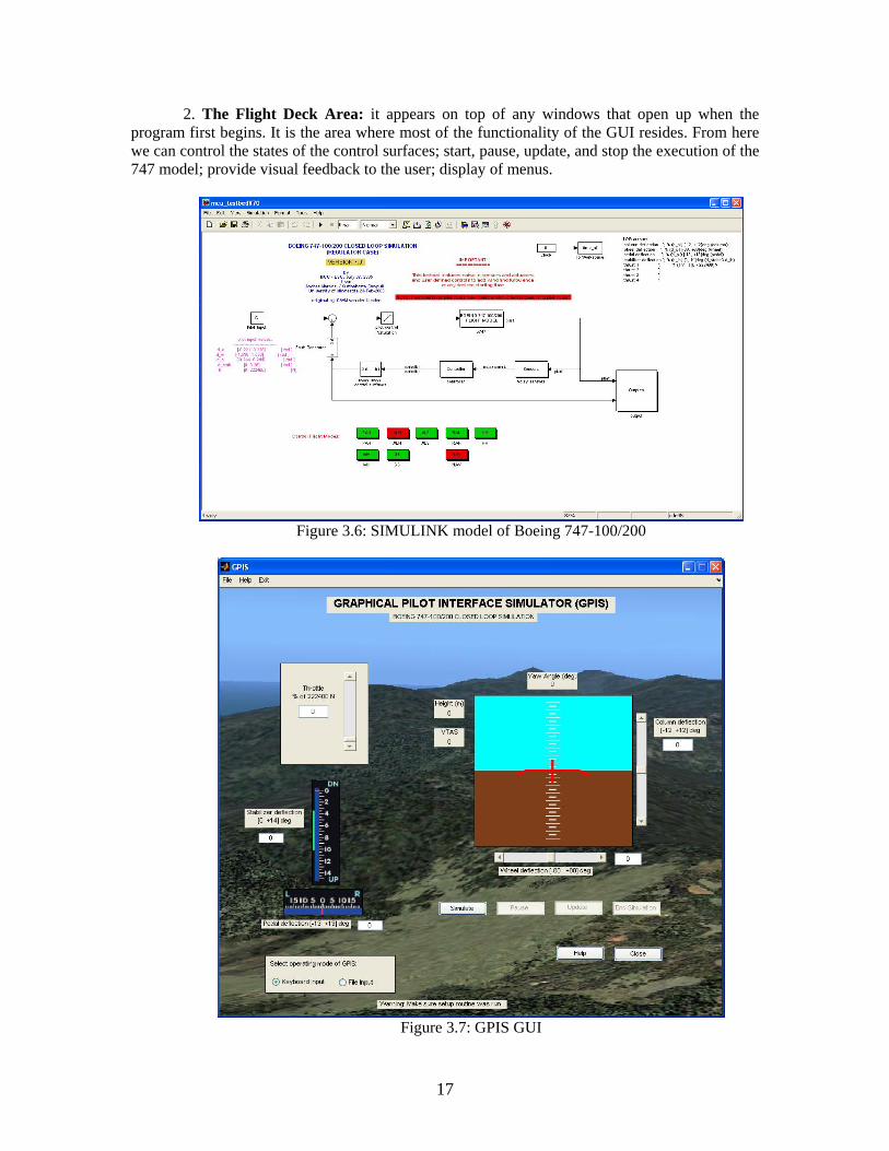
2. The Flight Deck Area: it appears on top of any windows that open up when the program first begins. It is the area where most of the functionality of the GUI resides. From here we can control the states of the control surfaces; start, pause, update, and stop the execution of the 747 model; provide visual feedback to the user; display of menus.

Figure 3.6: SIMULINK model of Boeing 747-100/200

Figure 3.7: GPIS GUI

17

The flight deck area contains controls, visual displays, and menus. A brief description of these elements follows:

• Menus: The menu bar is located on the top side of the flight deck area. It lists a few functions the GPIS GUI is not able to perform directly from what is visible to the user. This menu bar was created and can be modified with the Menu Editor. More details on the items in the menu can be found in Appendix A.

• Visual Displays: The main display elements developed in the GUI are the stabilizer and

rudder position displays and the attitude indicator. The stabilizer and rudder position display provides the user visual feedback of the relative position of the stabilizer/rudder deflection. The attitude indicator intends to emulate the attitude indicator of an airplane by providing pitch and bank visual information. It is the primary means by which a user is given visual feedback.

• Pilot Input Controls: These are the uicontrols that implement the ways the user is

allowed to exercise control of the simulation variables corresponding to actions a pilot takes in the plane. The inputs allowed result from the following input sources:

o Mouse input: allow movement of the sliders to the corresponding control

surface. o Keyboard control: permit direct user interaction. More details on the keyboard

strokes and corresponding action can be found in Appendix A. o Edit box key in: direct numerical manipulation of the allowable range for each

control surface may be typed in.

All forms of input provide the user a means of changing parameters within the allotted ranges.

• Simulator Controls: These are pushbutton uicontrols placed below the attitude indicator

that allow manipulation of the SIMULINK model running in the background. The pushbuttons available include Simulate, Pause, Update, End Simulation, Reset, Help, and Close. (Appendix A contains all details relating to their actions.) Pushbutton items that are displayed in light gray text are temporarily unavailable. They may not be available because of the state of the GPIS GUI. For example, the Pause pushbutton item will not be available if the model is not running.

• Operation Mode Control: The GPIS GUI has a section where the user can choose the

operation mode of the graphical user interface. These modes include:

o Keyboard Input: Also known as Default Mode, it runs the simulation by using keyboard inputs primarily. The other forms of control included under the Pilot Input Controls section, previously discussed, are also allowed.

o File Input: Run the simulation from a set of predefined variable inputs created by the user.

Please review Appendix A for details on using the GUI. A sample demo on running GPIS is included.

18

Chapter 4 Animations in MATLAB

Animations can provide us a great insight of the nature of the data in a manner that motionless data would not be able to grant. It is more natural for human beings to see objects in motion since we live in a very dynamic, constantly changing world. In this case we are simulating a dynamic object whose position and orientations are constantly changing.

This chapter describes what MATLAB allows us to do to produce simple animations; components of animation in our GPIS tool; and methods that we used to accomplish the goal of making animations come to life. 4.1 Animation Capabilities in MATLAB

MATLAB's graphic engine has the capability to create animations that can add to our visualization. It can do so in one of two methods, described as follows:

1. Frame-by-frame Capture and Playback: This method consists in creating several different figures, each stored as a single frame. To view the animation, the user must play it back as a movie. These types of animations are ideal for color-filled contours and 3-dimensional surface animations. For this project, this method fails to meet our requirements because it does not provide the real-time characteristic we are seeking to deliver.

2. On-the-fly Graphics Object Manipulation: Also known as Erase Mode method, this method is useful for line animations (i.e. computer graphics made of lines), where most of the plot remains the same. MATLAB achieves the animation effect by continually erasing and redrawing the object on the screen figure. Since this method meets the requirements of what this project is striving to achieve, we shall elaborate further on how it works to our advantage.

As we have seen, when a figure is created with all of its graphic objects included, a handles structure is created. The handles structure is used to change and modify the properties of an object. For any change in the properties of an object, the way the graphics engine in MATLAB is designed to work forces a redraw. Taking advantage of this behavior, we can program MATLAB to create different drawing effects. This is done in the EraseMode property of the figure handles. The possible inputs this field property can accept are as follows [4]:

• Normal: This is the default mode. As such, this mode completely redraws the affected region of the display. This mode produces the most accurate picture, but is the slowest. The other modes are faster, but do not perform a complete redraw making them less accurate.

• None: This method does not erase the objects as they are moved or modified. The object

remains visible on the screen as a trail.

19

• Background: For this method, MATLAB erases the object by redrawing it in the background color. This mode erases the object and anything below it. Method was tried but does not produce a very clean animation for us. Remnants of previous object are still visible.

• Xor: This mode erases only the object being modified, and it is usually is best for

animations, since remnants of previous graphics on the screen are no longer visible. For this project, the use of this technique will be quite extensive.

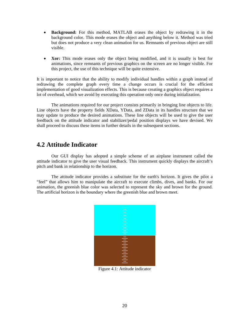
It is important to notice that the ability to modify individual handles within a graph instead of redrawing the complete graph every time a change occurs is crucial for the efficient implementation of good visualization effects. This is because creating a graphics object requires a lot of overhead, which we avoid by executing this operation only once during initialization. The animations required for our project consists primarily in bringing line objects to life. Line objects have the property fields XData, YData, and ZData in its handles structure that we may update to produce the desired animations. These line objects will be used to give the user feedback on the attitude indicator and stabilizer/pedal position displays we have devised. We shall proceed to discuss these items in further details in the subsequent sections. 4.2 Attitude Indicator Our GUI display has adopted a simple scheme of an airplane instrument called the attitude indicator to give the user visual feedback. This instrument quickly displays the aircraft’s pitch and bank in relationship to the horizon. The attitude indicator provides a substitute for the earth's horizon. It gives the pilot a “feel” that allows him to manipulate the aircraft to execute climbs, dives, and banks. For our animation, the greenish blue color was selected to represent the sky and brown for the ground. The artificial horizon is the boundary where the greenish blue and brown meet.

Figure 4.1: Attitude indicator

20

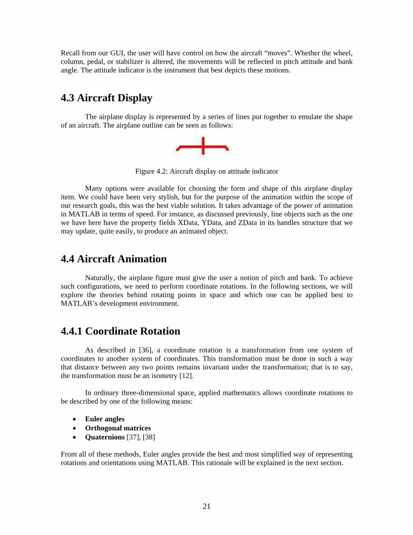
Recall from our GUI, the user will have control on how the aircraft “moves”. Whether the wheel, column, pedal, or stabilizer is altered, the movements will be reflected in pitch attitude and bank angle. The attitude indicator is the instrument that best depicts these motions. 4.3 Aircraft Display The airplane display is represented by a series of lines put together to emulate the shape of an aircraft. The airplane outline can be seen as follows:

Figure 4.2: Aircraft display on attitude indicator

Many options were available for choosing the form and shape of this airplane display

item. We could have been very stylish, but for the purpose of the animation within the scope of our research goals, this was the best viable solution. It takes advantage of the power of animation in MATLAB in terms of speed. For instance, as discussed previously, line objects such as the one we have here have the property fields XData, YData, and ZData in its handles structure that we may update, quite easily, to produce an animated object. 4.4 Aircraft Animation Naturally, the airplane figure must give the user a notion of pitch and bank. To achieve such configurations, we need to perform coordinate rotations. In the following sections, we will explore the theories behind rotating points in space and which one can be applied best to MATLAB’s development environment. 4.4.1 Coordinate Rotation As described in [36], a coordinate rotation is a transformation from one system of coordinates to another system of coordinates. This transformation must be done in such a way that distance between any two points remains invariant under the transformation; that is to say, the transformation must be an isometry [12]. In ordinary three-dimensional space, applied mathematics allows coordinate rotations to be described by one of the following means:

• Euler angles • Orthogonal matrices • Quaternions [37], [38]

From all of these methods, Euler angles provide the best and most simplified way of representing rotations and orientations using MATLAB. This rationale will be explained in the next section.

21

4.4.2 Euler Angles From [43], Euler angles are the means by which the relative position of coordinate systems may be described. They are the classical way of representing rotations in 3-dimensional Euclidean space. The advantage of Euler angles is that they split the complete rotation of a Cartesian coordinate system into three simpler rotations about the axes of this system [44]. For instance, note the following rotations in the x, y and z axes, respectively.

Figure 4.3: X-axis, Y-axis, and Z-axis rotation matrices [45]

A disadvantage of Euler angles that is worth noting is that when we store rotation as Euler angles, there can be tiny amounts of round off error [44].

Euler angles are used extensively in the classical mechanics of rigid bodies. In our case, the figure of the plane is treated as a rigid body pivoting, or rotating, about a point. On the other hand, for flight and aerospace engineers, they are even more useful since yaw, pitch, and roll correspond perfectly with the x, y, and z axes. Hence, our prevailing inclination to their use in the project is quite obvious. 4.4.3 Translation and Rotation

MATLAB provides us with some functions that allow for translation and rotation operations to be executed. Some of the techniques explored follow:

1. Rotate command: The rotate function rotates a graphics object in three-dimensional space, according to the right-hand rule. It is based on the rotation matrixes listed in Figure 4.3.

2. Hgtransform command: An hgtransform is an object in MATLAB used to group

items together. Objects of this category are usually parented to axes. The hgtransform allows us to transform objects as a group. For instance, to execute a translation or rotation, which is what we are interested in, in three-dimensional space, we simply perform one operation instead of one for every object contained in the group.

To achieve the aircraft animation, a combination of these techniques was implemented.

First, to attain the desired movements, the figure was defined as a group using hgtransform. This allowed us to take advantage of using the translation property of the hgtransform to produce the effect of pitch animation. On the other hand, the rotate command was issued to perform the effects of roll. For further details on how this was achieved, please refer to Appendix C. The expected output for the range of motions the previous method depicts are described as follows:

• Pitch*: The airplane figure is moved up or down. • Roll**: One wingtip moves up and the other down.

22

• Yaw**: Not depicted, only displayed as a numerical value, involves turning the plane left or right. In reality, no instrument is used to depict this motion in a cockpit.

* Positive pitch indicates plane is climbing. Negative pitch designates a descent. ** Positive roll/yaw is a turn to the right. A negative roll/yaw corresponds to a left turn. In addition, we assumed a zero rotation and translation condition refers to a straight and level flight path. 4.5 Stabilizer and Pedal Position Displays The Stabilizer and Pedal Position Displays, depicted in Figure 4.3, are used to give the user an idea of how much the stabilizer/pedal inputs have been deflected. The color scheme used is based on industry standards. Most liquid crystal displays (LCDs) in a cockpit use black as the default background color. Noticed on the stabilizer position display, a green neon color is used to indicate the normal deflection position of this pilot control input. Red is mostly for items that change, or things that are dynamic in nature (e.g. a stabilizer surface movement).

Figure 4.4: Stabilizer and rudder position displays, respectively

The above images were created using Paint, a simple picture editing software built into Windows. To be accurate with the animations, the images had to be developed using almost exact pixel measurements. This is because MATLAB tends to use pixels when working with images. (A pixel is equal to 1/72 of an inch.) [3]

Initially developed as a test bed for executing animations, we decided to keep these position indicators because they do not consume much of our computer resources. Additionally, their surface movement is limited to a narrow range and change little to none in any given flight condition. 4.6 Interacting with SIMULINK The key to animations is a continuous update of the screen display. When interfacing a GUI and SIMULINK, the best technique encountered involves the use of S-functions. The following sections describe what an S-function is and the advantages it provides to the programmer.

23

4.6.1 S-Functions An S-function is a SIMULINK block that allows us to build a general purpose function to perform any task we desire. S-functions have the flexibility of being built from various sources, including M-files, C, C++, ADA, FORTRAN, just to mention a few. S-functions can be used for many applications, such as [46]:

• Adding new general purpose blocks to SIMULINK. • Adding blocks that represent hardware device drivers. • Incorporating existing C code into a simulation. • Describing a system as a set of mathematical equations. • Using graphical animations.

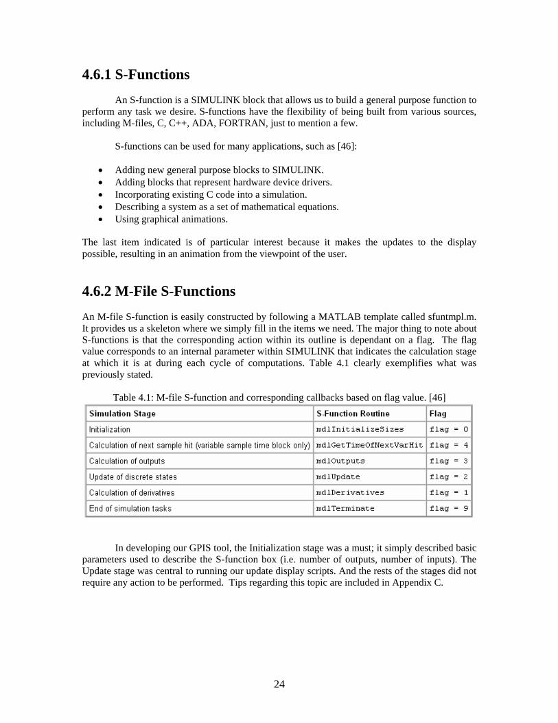
The last item indicated is of particular interest because it makes the updates to the display possible, resulting in an animation from the viewpoint of the user. 4.6.2 M-File S-Functions An M-file S-function is easily constructed by following a MATLAB template called sfuntmpl.m. It provides us a skeleton where we simply fill in the items we need. The major thing to note about S-functions is that the corresponding action within its outline is dependant on a flag. The flag value corresponds to an internal parameter within SIMULINK that indicates the calculation stage at which it is at during each cycle of computations. Table 4.1 clearly exemplifies what was previously stated.

Table 4.1: M-file S-function and corresponding callbacks based on flag value. [46]

In developing our GPIS tool, the Initialization stage was a must; it simply described basic parameters used to describe the S-function box (i.e. number of outputs, number of inputs). The Update stage was central to running our update display scripts. And the rests of the stages did not require any action to be performed. Tips regarding this topic are included in Appendix C.

24

Chapter 5 Conclusion In this project, we have described a tool that provides real-time simulation of a Boeing 747-100/200 using pilot command inputs. We have built the GPIS tool to provide FTLAB747 [1], [2], [28] an interactive front capable of delivering a more realistic flight simulation environment. Applications similar to GPIS demand a certain level of speed and realism. The techniques that have been developed here keep these requirements in mind. The main ideas we can itemize that have come from our research and tool development efforts are the following:

• Simulation is a more accurate tool to reflect dynamic systems, as it is an attempt to emulate the reality. It allows users to understand the interrelation between design and performance parameters, to identify potential problem areas, and so implement and test appropriate design modifications. By enabling the assessment of different scenarios, it is a powerful tool for assessing options, and as a result the final design is more precise.

• We have demonstrated the functionality and utility of using simulation as a tool for flight

simulation. Graphics allow us to focus on the interpretation of the results, as opposed to processing information. Through the use of graphics in simulation, more people can gain a better understanding of the systems being modeled.

• As the efficiency and flexibility of the code improves, simulation is becoming more

widely adopted for production systems. In addition, it offers flexibility and capacity for quick iteration.

• Chapters 3 and 4 provided a general guide about developing a GUI and basic animations

in MATLB. Understanding MATLAB’s programming environment, capabilities and limitations that were discussed are valuable information that may be extended to other model simulation and animation research projects.

Thus, we have demonstrated that a real time simulation environment can be developed

using MATLAB. We have increased the flexibility and the simulation power of the FTLAB747 tool. To my knowledge, this is the only tool of its kind associated with this model. 5.1 Summary of Contributions The main contributions of our work we can enumerate are as follows:

• Support the idea that simulation is effective.

• Test accuracy of the model.

• Provide a ‘tip’ guide to building GUIs and basic animations in MATLAB.

25

• Contribute a useful tool to allow more realistic flight conditions on our flight simulator

model.

• Explore the feature set built into the FTLAB747 model.

• Expand analysis capabilities of Boeing 747-100/200 SIMULINK model. 5.2 Limitations and Future Research This section mentions the major limitations of the research tool presented. We try to address these items with ideas for future work. This project suggests many directions to take on developing GUIs, creating animations, and the GPIS tool itself. The list of concerns we may propose includes, but is not limited to the following:

• The development of a tracking controller is strongly suggested. From reading [47], designing a tracking controller would seem like a very feasible addition to the model. A tracking controller would minimize input error and guarantee the pilot command inputs are accurately put into the system.

• Integrate GPIS to other software solutions to produce more dynamically real animations.

This would help increase the model’s utility more than what was presented in this project. For instance, the use of AVDS (Aviator Visual Design Simulator), a simulation tool for the development and evaluation of aircraft and flight control systems [49], has been suggested.

• The model includes components that will allow fault detection and correction

experiments to be carried out. This will take the pilot command inputs and FTC (fault tolerant control) / FDI (fault detection and isolation) to a higher level of practical testing. This also suggests the need for an additional user-friendly interface to address FTC/FDC studies.

• The current analysis methods (i.e. output graphs) provided by FTLAB747 are very

primitive. Since it was not the aim of this project to develop more advanced performance measures’ tools, we have replicated the same ones in FTLAB747 as a function called graph.m.

• Animation quality is subject to hardware components on which MATLAB is run. We

must keep in mind when an animation becomes too sluggish, its usefulness wanes; therefore, we must consider running it on a more powerful computer, such as Super Mike [48]. This will not only improve animation capabilities, but also allow faster, more accurate simulation replication and recurrence.

• The simulation software presented here has been optimized to the best of our knowledge.

As new techniques and options become available, the graphics routines developed here can be improved. Likewise, the software should support different hardware platforms that can provide the graphics horsepower to meet our modeling needs. Keep in mind, the GPIS tool was not run on other platforms (e.g. Linux, Mac).

26

• Another interesting possibility is to extend the animation manipulations done with GPIS

to quaternion theory. From our readings of [37], [38], they seem like a better choice since they are more natural to the flight testing area. In addition, they offer many advantages over Euler angles that might be worth investigating further in terms of practical use and functionality.

We hope the techniques introduced here allow others to achieve more interactive levels of simulation and higher level GUI animations. The advantages of simulation and visualization given to the scientists are unsurpassed by any other method.

27

Bibliography [1] Van Der Linden, C.A.A.M., DASMAT – Delft University Aircraft Simulation Model and Analysis Tool. Delft, 1996. Report LR-781, Technical University Delft. [2] M.H. Smaili. FLIGHTLAB 747 Benchmark for Advanced Flight Control Engineering v4.03. Delft, 1999. Technical University Delft. [3] P. Marchand and O.T. Holland, Graphics and GUIs with MATLAB, 3rd Edition, Chapman & Hall/CRC, 2003 [4] Mathworks, MATLAB support, Creating Graphical User Interfaces, [Online document], Available HTTP: http://www.mathworks.com/access/helpdesk/help/techdoc/creating_guis/creating_guis.html [5] Boeing, Jetliner Safety, [Online document], Available HTTP: http://www.boeing.com/commercial/safety/pf/pf_whatmakes.html [6] NASA, Aviation Safety and Security Program, [Online document], Available HTTP: http://avsp.larc.nasa.gov/program_saap.html [7] M.J. Harris, "Real-Time Cloud Simulation and Rendering," PhD dissertation, Department of Computer Science, University of North Carolina at Chapel Hill 2003, [8] Guided Flight Discovery, Instrument/Commercial Textbook, 2005, Jeppesen [9] Irvin N. Gleim, Pilot Handbook, Seventh Edition, 2003, Gleim [10] Fatalities by Accident Categories, Boeing,[Online reference], Available HTTP: http://www.boeing.com/commercial/safety/pf/pf_fatalities_by_accident_categories_cht.html [11] Mission Statement, Federal Aviation Administration, [Online reference], Available HTTP: http://www.faa.gov/about/mission/ [12] MSN Encarta, Microsoft, 2005, [Online encyclopedia], Available HTTP: http://encarta.msn.com/ [13] T. Schouwenaars , J. How and E. Feron, "Decentralized Cooperative Trajectory Planning of Multiple Aircraft with Hard Safety Guarantees", AIAA Guidance, Navigation, and Control Conference, Providence, RI, August 2004 [Online document], Available HTTP: http://gewurtz.mit.edu/papers/SHF04Aug.pdf [14] Technical Solutions, Solution 1-19J7T, MathWorks, 18 Apr 2005 [Online reference] Available HTTP: http://www.mathworks.com/support/solutions/data/ 1-19J7T.html?solution=1-19J7T

28

[15] MATLAB Central File Exchange, Fahad Al Mahmood, “msopen”, 2 Apr 2004, [Online code] Available HTTP: http://www.mathworks.com/matlabcentral/fileexchange/ loadFile.do?objectId=4562&objectType=file [16] Aircraft and Powerplant Corner, Boeing 747-Series, [Online reference], Available HTTP: http://home.swipnet.se/~w65189/transport_aircraft/b747/boeing_747_series.htm [17] Product Support, 1205 - Handles Graphics and Properties Guide, MathWorks, [Online manual], Available HTTP: http://www.mathworks.com/support/tech-notes/1200/1205.html [18] Wikipedia, Simulation, 3 Aug 2005, [Online reference], Available HTTP: http://en.wikipedia.org/wiki/Simulation [19] Simulation Based Tools, Importance of Simulation, [Online reference], Available HTTP: http://www.esru.strath.ac.uk/EandE/Web_sites/ 01-02/sim_mangmt/importance.htm [20] Flinders Meditech, Why is Simulation Training Important?, [Online reference], Available HTTP: http://www.flindersmeditech.com/sim_importance.html [21] J. Clark and G. Daigle, "The Importance of Simulation Techniques in ITS Research and Analysis", Proc. in Winter Simulation Conference, 1997, [Online document], Available HTTP: http://www.informs-sim.org/wsc97papers/1236.PDF [22] University at Buffalo, High Performance Computing and Computational Science, 2002, [Online reference], Available HTTP: http://www.cse.buffalo.edu/research-performance.shtml [23] Wikipedia, Scientific Computing, 28 Jul 2005, [Online reference], Available HTTP: http://en.wikipedia.org/wiki/Computational_science [24] Friedhoff, R. Mark, and W. Benzon, "Visualization, the Second Computer Revolution", Abrams 1989 [25] M. W. Rohrer, "Seeing is Believing: the Importance of Visualization in Manufacturing Simulation", Proc. in Winter Simulation Conference, 2000 [26] S. Wolfram and J. Schmidhuber, "A New Kind of Science", 2002 [27] J.W. Croft, "Refuse-To-Crash", Aerospace America, Mar 2003 [Online document], Available HTTP: http://avsp.larc.nasa.gov/images_saap_RTC.html [28] A. Marcos and G.J. Balas, "A Boeing 747-100/200 Aircraft Fault Tolerant and Fault Diagnostic Benchmark", Aerospace Engineering and Mechanics Department, University of Minnesota, June 2003 [29] T. Benson, "Aircraft Roatations",NASA Glenn Learning Technologies, 27 Feb 2004 [Online reference], Available HTTP: http://www.grc.nasa.gov/WWW/ K-12/airplane/rotations.html

29

[30] Airliners.net, Boeing 747 Cockpit, 28 Sept 2004, [Online image], Available HTTP: http://www.airliners.net/open.file/690415/M [31] MathWorks Documentation, "Simulink", [Online reference], Available HTTP: http://www.mathworks.com/access/helpdesk/help/toolbox/simulink/ [32] Princeton Satellite Systems, " Aircraft Control Toolbox Learning Edition", Nov 2004 [Online document], Available HTTP: http://www.psatellite.com/products/manuals/ACT_LEUsersGuide.pdf [33] MathWorks, "Building GUIs with MATLAB", Version 5, June 1997 [Online document], Available HTTP: http://www-ccs.ucsd.edu/matlab/pdf_doc/matlab/gui/buildgui.pdf [34] Omikron, "Building GUI in MATLAB: One Day Comprehensive Course", June 2005 [Online reference], Available HTTP: http://www.omikron.co.il/Products/Training/MATLAB_Courses/Building_GUI_in_MATLAB/ body_building_gui_in_matlab.html [35] J. Handal, screenshots, Microsoft Paint, 2005 [36] Wikipedia, "Coordinate Rotation", 1 May 2005 [Online reference], Available HTTP: http://www.absoluteastronomy.com/encyclopedia/c/co/coordinate_rotation.htm [37] Wikipedia, "Quaternion", 9 Aug 2005 [Online reference], Available HTTP: http://en.wikipedia.org/wiki/Quaternions [38] Wikipedia, "Quaternions and Spatial Rotation", 6 Aug 2005 [Online reference], Available HTTP: http://en.wikipedia.org/wiki/Quaternions_and_spatial_rotation [39] Eric W. Weisstein. "Quaternion", MathWorld, [Online reference], Available HTTP: http://mathworld.wolfram.com/Quaternion.html [40] NASA-Langely Research Center [Online reference] Available HTTP: http://www.nasa.gov/centers/langley/home/index.html [41] Dam, Koch, Lillholm, "Quaternions, Interpolation and Animation", 17 Jul 1998 [Online document], Available HTTP: http://www.diku.dk/publikationer/tekniske.rapporter/1998/98-5.ps.gz [42] Boeing Commercial Airplane Company, "747 Airplane Characteristics: Airport Planning", May 1984, [Online document], Available HTTP: http://www.boeing.com/assocproducts/aircompat/acaps/7471_toc.pdf [43] Wikipedia, "Euler Angles", 16 May 2005 [Online document], Available HTTP: http://en.wikipedia.org/wiki/Euler_angles

30

[44] M. Kraus, "LiveGraphics3D Example: Euler Angles", 28 February 1999 [Online document], Available HTTP: http://wwwvis.informatik.uni-stuttgart.de/~kraus/LiveGraphics3D/examples/Euler.html [45] Eric W. Weisstein. "Rotation Matrix." From MathWorld--A Wolfram Web Resource. [Online reference], Available HTTP: http://mathworld.wolfram.com/RotationMatrix.html [46] MathWorks, "Simulink Blocks: S-Function", [Online document], Available HTTP: http://www.mathworks.com/access/helpdesk/help/toolbox/simulink/slref/slref.html [47] F. Liao, J.L. Wang, G. Yang, "Reliable Robust Flight Tracking Control: An LMI Approach", January 2002, IEEE Transactions on Control Systems Technology, Vol. 10, No. 1 [48] LSU Center for Applied Information Technology and Learning, “SuperMike: LSU’s World-class Supercomputer”, [Online reference], Available HTTP: http://www.phys.lsu.edu/faculty/tohline/capital/beowulf.html [49] RasSimTech Home, [Online Reference], Available HTTP: http://www.rassimtech.com

31

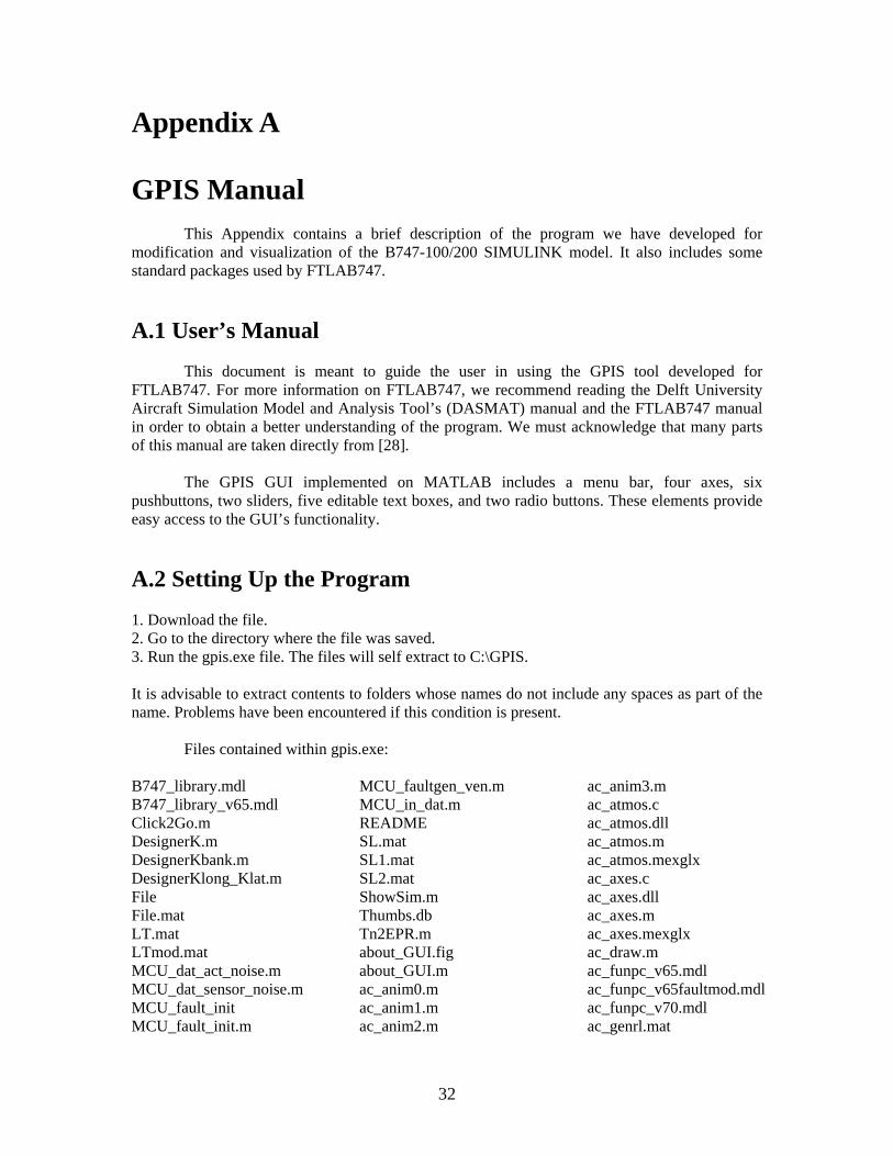
Appendix A GPIS Manual This Appendix contains a brief description of the program we have developed for modification and visualization of the B747-100/200 SIMULINK model. It also includes some standard packages used by FTLAB747. A.1 User’s Manual

This document is meant to guide the user in using the GPIS tool developed for FTLAB747. For more information on FTLAB747, we recommend reading the Delft University Aircraft Simulation Model and Analysis Tool’s (DASMAT) manual and the FTLAB747 manual in order to obtain a better understanding of the program. We must acknowledge that many parts of this manual are taken directly from [28].

The GPIS GUI implemented on MATLAB includes a menu bar, four axes, six

pushbuttons, two sliders, five editable text boxes, and two radio buttons. These elements provide easy access to the GUI’s functionality.

A.2 Setting Up the Program 1. Download the file. 2. Go to the directory where the file was saved. 3. Run the gpis.exe file. The files will self extract to C:\GPIS. It is advisable to extract contents to folders whose names do not include any spaces as part of the name. Problems have been encountered if this condition is present.

Files contained within gpis.exe:

B747_library.mdl B747_library_v65.mdl Click2Go.m DesignerK.m DesignerKbank.m DesignerKlong_Klat.m File File.mat LT.mat LTmod.mat MCU_dat_act_noise.m MCU_dat_sensor_noise.m MCU_fault_init MCU_fault_init.m

MCU_faultgen_ven.m MCU_in_dat.m README SL.mat SL1.mat SL2.mat ShowSim.m Thumbs.db Tn2EPR.m about_GUI.fig about_GUI.m ac_anim0.m ac_anim1.m ac_anim2.m

ac_anim3.m ac_atmos.c ac_atmos.dll ac_atmos.m ac_atmos.mexglx ac_axes.c ac_axes.dll ac_axes.m ac_axes.mexglx ac_draw.m ac_funpc_v65.mdl ac_funpc_v65faultmod.mdl ac_funpc_v70.mdl ac_genrl.mat

32

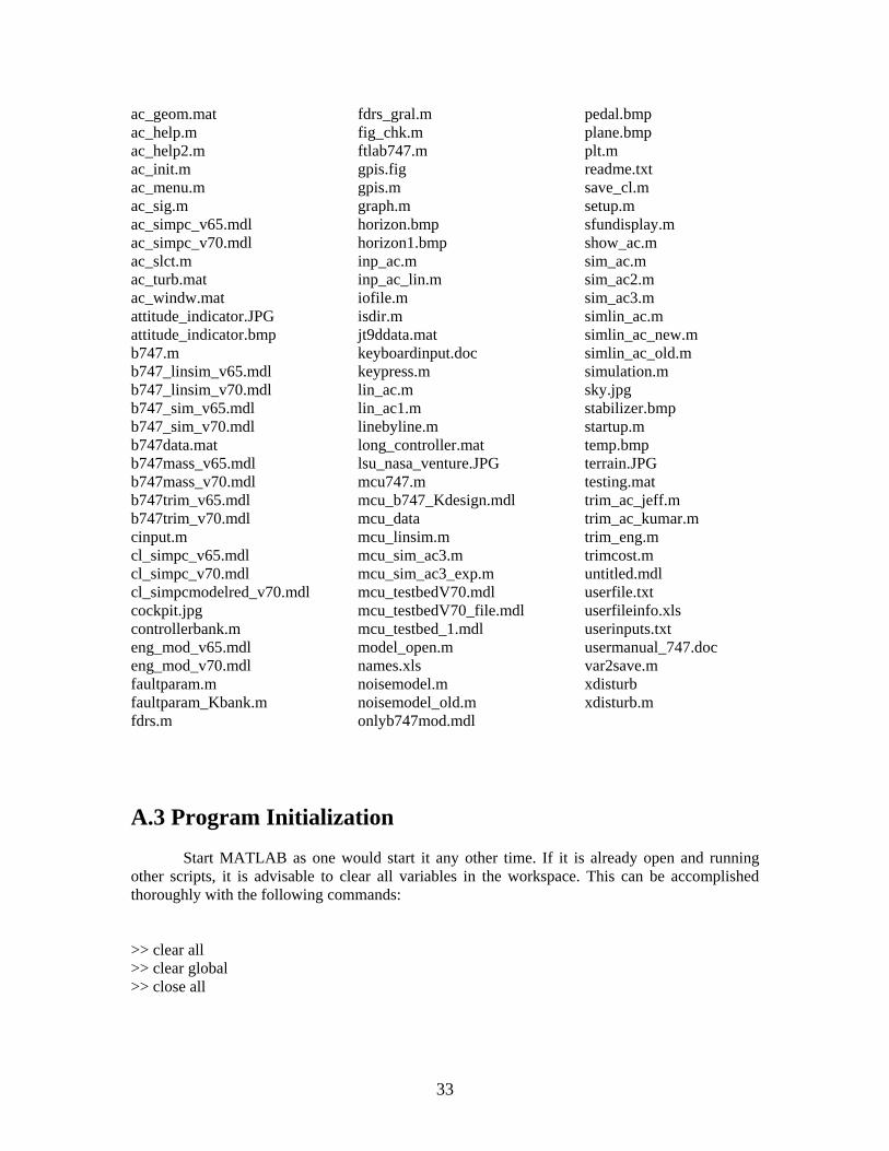
pedal.bmp fdrs_gral.m ac_geom.mat plane.bmp fig_chk.m ac_help.m plt.m ftlab747.m ac_help2.m readme.txt gpis.fig ac_init.m save_cl.m gpis.m ac_menu.m

ac_sig.m setup.m graph.m sfundisplay.m horizon.bmp ac_simpc_v65.mdl show_ac.m horizon1.bmp ac_simpc_v70.mdl sim_ac.m inp_ac.m ac_slct.m sim_ac2.m inp_ac_lin.m ac_turb.mat sim_ac3.m iofile.m ac_windw.mat simlin_ac.m isdir.m attitude_indicator.JPG simlin_ac_new.m jt9ddata.mat attitude_indicator.bmp simlin_ac_old.m keyboardinput.doc b747.m simulation.m keypress.m b747_linsim_v65.mdl sky.jpg lin_ac.m b747_linsim_v70.mdl stabilizer.bmp lin_ac1.m b747_sim_v65.mdl startup.m linebyline.m b747_sim_v70.mdl temp.bmp long_controller.mat b747data.mat terrain.JPG lsu_nasa_venture.JPG

mcu747.m b747mass_v65.mdl

testing.mat b747mass_v70.mdl trim_ac_jeff.m mcu_b747_Kdesign.mdl b747trim_v65.mdl trim_ac_kumar.m mcu_data b747trim_v70.mdl trim_eng.m mcu_linsim.m cinput.m trimcost.m mcu_sim_ac3.m cl_simpc_v65.mdl untitled.mdl mcu_sim_ac3_exp.m cl_simpc_v70.mdl userfile.txt mcu_testbedV70.mdl cl_simpcmodelred_v70.mdl userfileinfo.xls mcu_testbedV70_file.mdl cockpit.jpg userinputs.txt mcu_testbed_1.mdl controllerbank.m usermanual_747.doc model_open.m eng_mod_v65.mdl var2save.m names.xls eng_mod_v70.mdl xdisturb noisemodel.m faultparam.m xdisturb.m noisemodel_old.m faultparam_Kbank.m onlyb747mod.mdl fdrs.m

A.3 Program Initialization

Start MATLAB as one would start it any other time. If it is already open and running other scripts, it is advisable to clear all variables in the workspace. This can be accomplished thoroughly with the following commands: >> clear all >> clear global >> close all

33

The next step is to assure that MATLAB is in the correct directory for the program to run. This should be done as follows:

1. Change the directory to GPIS. 2. Type at the MATLAB prompt: >> cd C:\GPIS A.3.1 Trimming the Aircraft The first thing to do is to trim the aircraft at a specific point of the flight envelope. Running the setup.m file takes the user through the trim routine similar to that of FTLAB747. A trim is necessary to prepare the model for execution and modification by our GPIS tool. The GUI will start and the user will have the option to make changes or start the simulation. The first part of the setup routine sets the weight and balance prerequisites of the airplane. This is depicted by the screenshot in Figure A.1:

Figure A.1: Weight and balance setup of airplane

Once this is done, the next screen will ask for the configuration point and flight

condition. The configuration point is determined by the altitude and Mach number. Depending which flight condition was selected, the program will ask you for different parameters (e.g. FPA = Flight Path Angle, n = load factor, sideslip angle). Refer to the DASMAT manual [1] for more information.

34

Figure A.2: Configuration point and flight condition

After the trimming is achieved the values obtained are shown (Figure A.3). It is important

to note that it is not always possible to trim the aircraft at all flight conditions. Before starting, some engineering decisions should be made, such as what kind of flight envelope and conditions will be of interest and possible to achieve. Note: Flight conditions 5 and 6, beta-trim and specific-power-turn respectively, are not reliable in any of the FTLAB747 versions.

Figure A.3: Trim conditions results

After the trimming subroutine has ended the user is allowed to determine if faults should

be introduced into the system. This item is a topic of advanced research left to those after us. Finally, our GPIS tool is launched, with the SIMULINK model in the background. The sections that follow are intended to provide the user with basic use and description of the parts developed for the GPIS tool.

35

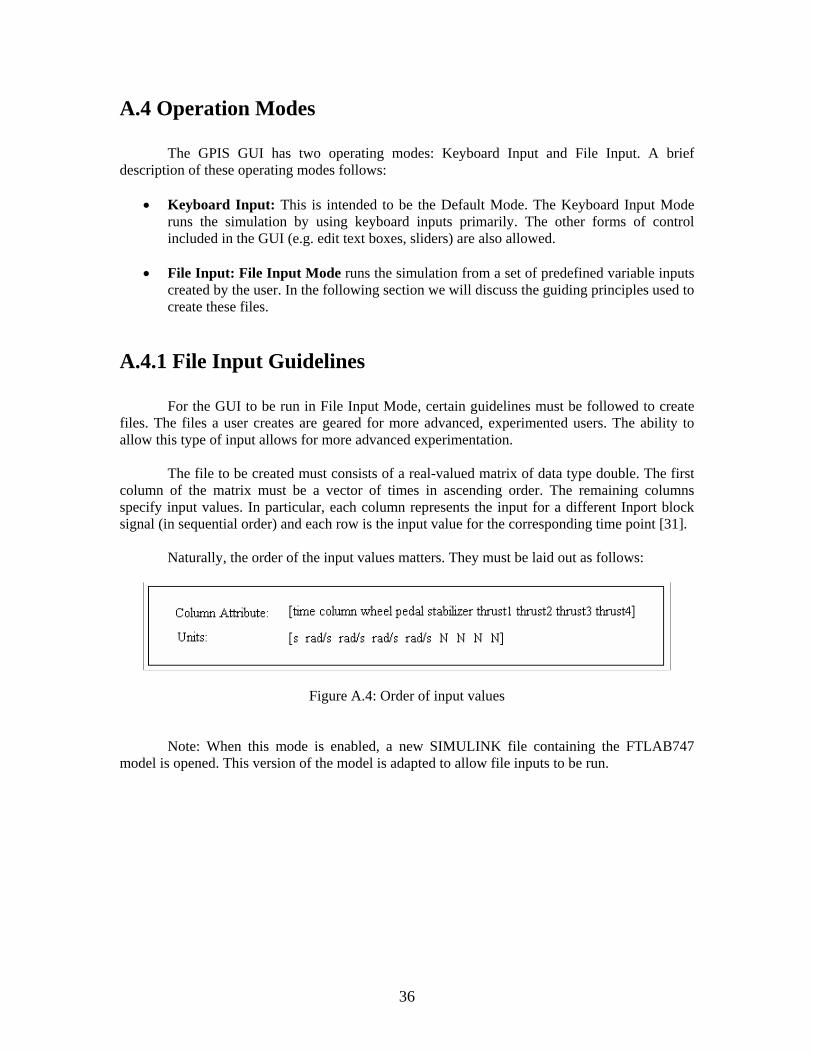
A.4 Operation Modes The GPIS GUI has two operating modes: Keyboard Input and File Input. A brief description of these operating modes follows:

• Keyboard Input: This is intended to be the Default Mode. The Keyboard Input Mode runs the simulation by using keyboard inputs primarily. The other forms of control included in the GUI (e.g. edit text boxes, sliders) are also allowed.

• File Input: File Input Mode runs the simulation from a set of predefined variable inputs

created by the user. In the following section we will discuss the guiding principles used to create these files.

A.4.1 File Input Guidelines For the GUI to be run in File Input Mode, certain guidelines must be followed to create files. The files a user creates are geared for more advanced, experimented users. The ability to allow this type of input allows for more advanced experimentation. The file to be created must consists of a real-valued matrix of data type double. The first column of the matrix must be a vector of times in ascending order. The remaining columns specify input values. In particular, each column represents the input for a different Inport block signal (in sequential order) and each row is the input value for the corresponding time point [31]. Naturally, the order of the input values matters. They must be laid out as follows:

Figure A.4: Order of input values Note: When this mode is enabled, a new SIMULINK file containing the FTLAB747 model is opened. This version of the model is adapted to allow file inputs to be run.

36

A.5 Menu Bar The GPIS GUI contains three menus: File, Help, and Exit. The options provided in each menu are described in the section that follows.

o File Menu:

The File menu includes the following options:

• Setup Simulator… Sets GPIS to a starting point.

• Background… Allows user to switch background image.

• Print Print snapshot of GUI’s present state.

• Print Setup Configure print options.

• Save Saves output generated by SIMULINK model into a file.

• Close Closes GPIS.

o Help Menu: The Help menu includes the following options:

• Keyboard Inputs Opens document containing table of operable keys.

• User Manual Opens User Manual PDF document.

• About GPIS Displays the GPIS version information.

o Exit Menu: The Exit menu does not have any options. It simply closes the GPIS and all associated figures, including the SIMULINK windows. A.6 Pushbuttons The GPIS GUI contains several pushbuttons: Simulate, Pause, Update, End Simulation, Reset, Help, and Close. The actions performed by each pushbutton are described in the section that follows.

• Simulate Start simulation in the background SIMULINK model.

• Pause Pause SIMULINK model.

37

• Update Pause SIMULINK model, update, and then continue.

• End Simulation Stop SIMULINK model; save simulated flight.*

• Reset Retune SIMULINK model to starting parameters.

• Help Open PDF document with this help reference.

• Close Close all windows, including SIMULINK and GPIS. * Once the simulation is over, the user is given the possibility of saving the simulated flight. The results may later be analyzed with the plot utility graph.m A.7 Pilot Control Inputs The following table summarizes the access a user has using a keyboard to manipulate the model. The keys selected are a product of location and ease of operability for the user.

Table A.1: Pilot keyboard actions. Keyboard

Stroke: Action: Aircraft Change:

Up Arrow Dive Elevator surface raised. Decrease angle of attack.

Down arrow Climb Elevator surface lowered. Increase angle of attack

Left Arrow Left turn Left aileron up. Right aileron down. Right Arrow Right turn Right aileron up. Left aileron down. Minus Sign (-) Speed down Throttle decrease. Plus Sign (+) Speed up Throttle increase. A Slight dive Stabilizer surface angle decreased. Z Slight climb Stabilizer surface angle increased. Q Nose shift left Rudder surface deflected left. W Nose shift right Rudder surface deflected right. Space Bar Update SIMULINK model None.

** The mouse may be used to change parameters by adjusting the sliders. Typing in the editable text boxes allows for user input also. A.8 Other Aids for User Keeping the design of GPIS as user friendly as possible, other forms of aid incorporated into this research tool include:

• ToolTipString property: It is a property of certain uicontrols that allows the programmer to specify, in the form of text, tips to the user regarding the associated

38

uicontrol. It is activated when the user moves the mouse pointer over the control and leaves it there, tool tip is displayed.

• Help pushbutton: Performs same action as the Keyboard Inputs and User Manual fields

under the Help menu, except information is bundled up into single PDF file.

• Help menu: contents previously described. A.9 Feedback For comments, suggestions, and general feedback feel free to send an email to the following address: [email protected].

39

Appendix B Conventions

In this report we have used following conventions: B.1 Coordinate System for Attitude Indicator

We use a right-handed coordinate system. In computer graphics it is common to use a left-handed coordinate system. This allows the z-axis to point ``into'' the screen which seems natural. Since the rotation methods used primarily coordinates for mathematical derivations, we have chosen to use the mathematical standard --- the right-handed coordinate system. B.2 Rotation

Still using the mathematical standard, we rotate counter-clockwise. The direction of rotation about an axis is obtained by the right-hand rule: Hold the axis with right hand and the thumb pointing in the positive direction of the axis. A positive rotation will now rotate in the direction of the fingers (apart from the thumb). This is illustrated below:

Figure B.1: Coordinate system for rotations [41]

B.3 Pilot Control Sign Convention From the use of FTLAB747, the sign convention must remain the same and, as described in [28], is as follows:

• Column deflection: A positive deflection (towards the pilot) yields a positive body pitching moment. A negative deflection (away from the pilot) produces a negative body pitching moment.

• Stabilizer deflection: It produces similar effects to the column deflection in terms of

body pitching input.

• Wheel deflection: A positive wheel deflection is equivalent to a clockwise rotation. • Pedal deflection: Similar to wheel when either right/left pedal is pressed respectively.

40

Appendix C Implementation Tips Appendix C highlights a few items worth noting that allowed for the completion of this project. They may be regarded as tips to be used by others as required.

• Initializing GUIs:

Every time a GUI is run, a function referred to as the ‘Opening Function’ is executed before the GUI is visible to the user. It is here where we perform tasks that need to be completed before the user accesses the GUI. For example, some of the actions that should be performed here are: initialization of displays, creation of variables, reading data from base workspace.

Following is an example where a function is called to set background display of GUI variables.

function gpis_OpeningFcn(hObject, eventdata, handles, varargin)

% Choose default command line output for gpis handles.output = hObject;

% Initialize values handles.Geaux = 0; %do not activate keyboard handles.pilot = [0 0 0 0 0 0 0 0]; % Initialize Displays

% Initialize background: name = 'terrain.jpg'; %default background handles = initialize_background(hObject, handles, name);

{other functions}

%Update handles structure guidata(hObject, handles);

Also, we need to note the assignment of variables used by the GUI. The other lines of code (i.e. handles.output and guidata) noted are standard for all GUI opening functions.

• Slider-edit box link:

This tip greatly emphasizes the flexibility that the handles structure gives the programmer when working with GUIs. As we will see next, the snippet of code provided shows how the slider and edit text box are interconnected.

41

Edit text box callback: function wheel_edit_Callback(hObject, eventdata, handles) %hObject refers to edit box

% Obtain value placed in edit box disp_wheel= str2double(get(handles.wheel_edit,'String'));

% Determine whether disp_wheel iswthin range If isnumeric(disp_wheel) & ...

disp_wheel >= get(handles.wheel_slider,'Min') & ... disp_wheel <= get(handles.wheel_slider,'Max') % Display entered value in edit box set(hObject,'String', disp_wheel); % Place value for slider set(handles.wheel_slider,'Value',disp_wheel); else {issue some error message or some adjustment}

Slider callback:

function wheel_slider_Callback(hObject, eventdata, handles) set(handles.wheel_edit,'String',num2str(get(handles.wheel_slider,'Value')));

They rely on each others property fields to get and set information. The use of the handles structure passed to each callback function makes this quite easy.

• Mouse-keyboard recognition: Each figure created in MATLAB has a particular set of properties associated with it. Of

particular interest for us are the KeyPressFcn and WindowButtonDownFcn fields. These property fields allow the name of an M-file to be defined. This means that every time a mouse button is clicked over the figure or a key is pressed when the window is active, MATLAB will execute the M-file in the KeyPressFcn or WindowButtonDownFcn property, accordingly. For instance, note the following exerpt from keypress.m (Appendix D):

key = double(get(handles.output,'CurrentCharacter')); % get key pressed if key = 28 %left arrow {execute code for left arrow action} Note that keypress.m relies on CurrentCharacter property to inquire what key was pressed from the keyboard. The key assignments used by MATLAB are standard ASCII code key assignments.

• Figure property manipulation for animations:

MATLAB offers many operating options that can be molded to our specific needs. In our case, we needed to make GPIS efficient at producing animations that were not ‘sluggish’. To do so, a variety of property fields were changed to achieve the objective. Other than the options discussed in this text, other options discovered to be useful included the following:

42

o BackingStore: off

Also known as off screen pixel buffer [4], it is set to “off” to reduce memory consumption. It allows the speed of animations to be increased because it eliminates the need to draw the figure both on and off the screen.

o DoubleBuffer: on As defined in [3], double buffering is the process of drawing to an off-screen pixel buffer and

then copying the buffer contents to the screen once the drawing is complete. Setting double buffering to “on” generally produces flash-free rendering for simple animations.

o IntegerHandle: off

MATLAB generally stores figure handles as integers. Turning IntegerHandles to the off position makes MATLAB assign non-reusable real numbers (e.g. 34.00235) to the handles instead. The advantage of doing this is to reduce the likelihood of inadvertently drawing into other GUI figures, such as dialog boxes.

o Renderer: painters

This property allows the programmer to select a method used by MATLAB to render graphics for the screen and printing. MATLAB allows for three methods: painters, zbuffer, and OpenGL. The fastest method is OpenGL, since it enables MATLAB to access graphics hardware that is available on some systems [3]. For simple graphics, such as the ones encountered in this project, painters suffices.

• Making an hgtransform group: Hgtransform is a MATLAB function for graphics that’s allows a group of objects to be

considered as a single entity. This is done by parenting objects to a single “hgtransform” object. For example, % Create an hgtransform object: handles.transform = hgtransform('Parent',handles.horizon_axes); % Set paret:t set(handles.line,'Parent',handles.transform); The main advantage of parenting objects to an hgtransform object is that it provides the ability to perform a single action (e.g. rotation or translation) on the child objects in unison. The end result is to save processing time, which results in very efficient programming.

43

• Translation and rotation of aircraft figure: Hgtransform has a sister function, makehgtform, which allows for translation operations to be

computed. The translation about the y axis portrays a pitch application. The matrix used for such computation follows:

Figure C.1: Translation about the y-axis. ‘y’ corresponds to the pitch angle in degrees.

To perform a translation of an hgtransform group, its Matrix field property is manipulated as we can see in the following code:

% Translate takes you directly to pitch angle desired.

pitch = makehgtform('translate',[0 anglep 0]); set(handles.transform,'Matrix',pitch); The rotation command applied to the whole figure allows for the roll angle to be depicted.

Keep in mind the rotation to perform is about the z-axis, since we are limited to a two dimensional view by the computer screen.

The basic fact to using the rotate command appropriately is not to confuse the direction of the

axes. For instance, a roll to the right was defined as a positive angle, while a negative roll angle is a left turn. Another key factor was to store, compare, and make absolute comparisons between the current angle and the current one computed by each SIMULINK cycle. These ingenious steps can be noted in the following code fragment:

angle_roll = rad2deg(handles.xobs(7)); % new rotation angle % previous rotation angle rotation_angle = get(handles.line(1),'UserData'); center = [100 100 0]; zdir = [0 0 1]; % axis about which we rotate if rotation_angle > angle_roll angle = - abs(rotation_angle - angle_roll); if angle_roll < 0 rotate(handles.line,zdir,-angle, center); else rotate(handles.line,zdir,-angle, center); end set(handles.line(1),'UserData', (rotation_angle + angle)); elseif rotation_angle < angle_roll angle = abs(angle_roll - rotation_angle); if angle_roll < 0 rotate(handles.line,zdir,angle, center);

44

else rotate(handles.line,zdir,-angle, center); end set(handles.line(1),'UserData', (rotation_angle + angle)); else angle = 0; rotate(handles.line,zdir,angle, center); set(handles.line(1),'UserData',rotation_angle); end

• Pixel units for the axes:

A key concept in creating exact animations, as the ones required by this tool, is the use of pixels as the measurement units. Using any image editing program, such as Microsoft Paint, images (e.g. the attitude indicator or the stabilizer position display) must be done by means of exact pixel dimensional. The rational to doing this is that each pixel is viewed as an element in a matrix, which is MATLAB’s means of operation.

To make our pixel units match how MATLAB interprets the image on the computer screen,

the Units property field must be selected to ‘pixels’ for them to match up correctly.

• S-function callback method options:

Selection of the stage to execute code plays a very important role in how the GUI-

SIMULINK relationship works. To exemplify our warning, deciding which flag to select for running the update-display routine for the GUI was determined by trial and error. The lesson learned dictates that the display-update routine must be done when a flag of value 2 (Update stage) is issued. Our first thoughts lead us to choose a flag of value 3 (Output stage) initially. This proved to be problematic because the GUI figure would lose its status of being the current figure. The consequences of this broke our keyboard input capabilities. At flag value of 2, optimal animation display is maintained, GUI figure remains active, and our simulation runs according to our intentions.

45

Appendix D MATLAB Source Code Included is MATLAB code developed for GPIS GUI. Modifications done to files from FTLAB747 not included. setup.m %%%%%%%%%%%%%%%%%%%%%%%%%%%%%%%%%%%%%%%%%%%%%%%%%%%%%%%%%%%%%%%%%%%%%%%%%%%%%%%%%%%%%%% % PROGRAM NAME: Graphical Pilot Interface Simulator GUI Coding started: 01/19/05 % Last revision: 08/24/05 % % % PURPOSE: Setup Simulink model and initialize GPIS GUI % % % FUNCTIONS USED : Various functions from ftlab747 customized for our % purposes, gpis % % REMARKS: Matlab 6.5 can be used. %%%%%%%%%%%%%%%%%%%%%%%%%%%%%%%%%%%%%%%%%%%%%%%%%%%%%%%%%%%%%%%%%%%%%%%%%%%%%%%%%%%%%%% clear all close all % Create variable in base workspace pilot = [0 0 0 0 0 0 0 0 ]; % pilot = [ column wheel pedal stabilizer thrust1 thrust2 thrust3 trust4] % Initialization: clc; simrun = []; % Variable to run simulaton from file. trimval = 1; sim_flag = 1; ac_init; % Setup Simulink model trim_ac_jeff; % Check for crucial variables to set starting point for GPIS: if ~exist('u0','var') | ~exist('Tn0','var')| ~exist('x0','var') errordlg('Variables missing u0, Tn0, and x0.', 'Trim File Error'); else variables_exist = 1; end % Give control to GUI gpis;

46

Click2Go.m %%%%%%%%%%%%%%%%%%%%%%%%%%%%%%%%%%%%%%%%%%%%%%%%%%%%%%%%%%%%%%%%%%%%%%%%%%%%%%%%%%%%%%% % FUNCTION NAME: Click2Go Coding started: 01/19/05 % Last revision: 07/23/05 % % PURPOSE: Activate display. % % ACTIONS: Gets current GUI information, makes keyboard active, % and updates GUI. % % % REMARKS: Matlab 6.5 can be used. %%%%%%%%%%%%%%%%%%%%%%%%%%%%%%%%%%%%%%%%%%%%%%%%%%%%%%%%%%%%%%%%%%%%%%%%%%%%%%%%%%%%%%% function Click2Go handles = guidata(gcf); % Allow action to start handles.Geaux = 1; % Update handles structure guidata(gcf,handles);

47

keypress.m %%%%%%%%%%%%%%%%%%%%%%%%%%%%%%%%%%%%%%%%%%%%%%%%%%%%%%%%%%%%%%%%%%%%%%%%%%%%%%%%%%%%%%% % FUNCTION NAME: keypress Coding started: 01/19/05 % Last revision: 08/24/05 % % % PURPOSE: Read keyboard input from user and perform requested action. % % KEY ACTIONS: Up decrease column angle % Down increase column angle % Right increase wheel angle % Left decrease wheel angle % - decrease thrust % + increase thrust % q decrease pedal angle % w increase pedal angle % a decrease stabilizer angle % z increase stabilizer angle % Space Bar update model % % REMARKS: Matlab 6.5 can be used. %%%%%%%%%%%%%%%%%%%%%%%%%%%%%%%%%%%%%%%%%%%%%%%%%%%%%%%%%%%%%%%%%%%%%%%%%%%%%%%%%%%%%%% function keypress handles = guidata(gcf); if handles.Geaux % make sure that figure is active window key = double(get(handles.output,'CurrentCharacter')); % get key pressed if key == 28 %left arrow val = get(handles.wheel_slider,'Value'); val = val - 2; if val >= get(handles.wheel_slider,'Min') & val <= get(handles.wheel_slider,'Max') set(handles.wheel_edit,'String',num2str(val));% set string for text edit box set(handles.wheel_slider,'Value',val);% set value for slider to update % Store changed attribute handles.pilot(2) = deg2rad(val); assignin('base','pilot',handles.pilot); end elseif key == 29 %right arrow val = get(handles.wheel_slider,'Value'); val = val + 2; if val >= get(handles.wheel_slider,'Min') & val <= get(handles.wheel_slider,'Max') set(handles.wheel_edit,'String',num2str(val));% set string for text edit box set(handles.wheel_slider,'Value',val);% set value for slider to update % Store changed attribute handles.pilot(2) = deg2rad(val); assignin('base','pilot',handles.pilot); end elseif key == 30 %up arrow val = get(handles.column_slider,'Value'); val = val - 0.5; if val >= get(handles.column_slider,'Min') & val <= get(handles.column_slider,'Max') set(handles.column_edit,'String',num2str(val));% set string for text edit box set(handles.column_slider,'Value',val);% set value for slider to update % Store changed attribute handles.pilot(1) = deg2rad(val); assignin('base','pilot',handles.pilot); end elseif key == 31 %down arrow val = get(handles.column_slider,'Value'); val = val + 0.5; if val >= get(handles.column_slider,'Min') & val <= get(handles.column_slider,'Max')

48

set(handles.column_edit,'String',num2str(val));%set string for text edit box set(handles.column_slider,'Value',val);%set value for slider to update % Store changed attribute handles.pilot(1) = deg2rad(val); assignin('base','pilot',handles.pilot); end elseif key == 113 | key == 81 %q key val = str2num(get(handles.pedal_edit,'String')); deflection_range = get(handles.pedal_edit,'UserData'); % deflection range val = val - 0.5; if val >= deflection_range(1) & val <= deflection_range(2) set(handles.pedal_edit,'String',num2str(val));% set string for text edit box % Update stabilizer animation: axes(handles.pedal_axes); hold on; pedal_x = 68 + (val * 3.3); set(handles.pedal_line,'XData',[pedal_x, pedal_x]); drawnow; hold off; % Store changed attribute handles.pilot(3) = deg2rad(-val); assignin('base','pilot',handles.pilot); end elseif key == 119 | key == 87 %w key val = str2num(get(handles.pedal_edit,'String')); deflection_range = get(handles.pedal_edit,'UserData'); % deflection range val = val + 0.5; if val >= deflection_range(1) & val <= deflection_range(2) set(handles.pedal_edit,'String',num2str(val));% set string for text edit box % Update stabilizer animation: axes(handles.pedal_axes); hold on; pedal_x = 68 + (val * 3.3); set(handles.pedal_line,'XData',[pedal_x, pedal_x]); drawnow; hold off; % Store changed attribute handles.pilot(3) = deg2rad(-val); assignin('base','pilot',handles.pilot); end elseif key == 97 | key == 65 %a key val = str2num(get(handles.stabilizer_edit,'String')); deflection_range = get(handles.stabilizer_edit,'UserData'); val = val - 0.5; if val >= deflection_range(1) & val <= deflection_range(2) set(handles.stabilizer_edit,'String',num2str(val));% set string for text edit box % Update stabilizer animation: axes(handles.stabilizer_axes); hold on; stabilizer_y = 18.75 + (val * 10.1); set(handles.stabilizer_line,'YData',[stabilizer_y, stabilizer_y]); drawnow; hold off; % Store changed attribute handles.pilot(4) = deg2rad(val); assignin('base','pilot',handles.pilot); end elseif key == 122 | key == 90 %z key val = str2num(get(handles.stabilizer_edit,'String')); deflection_range = get(handles.stabilizer_edit,'UserData'); val = val + 0.5; if val >= deflection_range(1) & val <= deflection_range(2) set(handles.stabilizer_edit,'String',num2str(val));%set string for text edit box

49

% Update stabilizer animation: axes(handles.stabilizer_axes); hold on; stabilizer_y = 18.75 + (val * 10.1); set(handles.stabilizer_line,'YData',[stabilizer_y, stabilizer_y]); drawnow; hold off; % Store changed attribute handles.pilot(4) = deg2rad(val); assignin('base','pilot',handles.pilot); end elseif key == 45 %- key val = get(handles.throttle_slider,'Value'); val = val - 1; if val >= get(handles.throttle_slider,'Min') & val <= get(handles.throttle_slider,'Max') set(handles.throttle_edit,'String',num2str(val));% set string for text edit box set(handles.throttle_slider,'Value',val);% set value for slider to update % Value of thrust in Newtons N = (val / 100 ) * 222400; % Store changed attribute handles.pilot(5:8) = N; assignin('base','pilot',handles.pilot); end elseif key == 43 %+ key val = get(handles.throttle_slider,'Value'); val = val + 1; if val >= get(handles.throttle_slider,'Min') & val <= get(handles.throttle_slider,'Max') set(handles.throttle_edit,'String',num2str(val));% set string for text edit box set(handles.throttle_slider,'Value',val);% set value for slider to update % Value of thrust in Newtons N = (val / 100 ) * 222400; % Store changed attribute handles.pilot(5:8) = N; assignin('base','pilot',handles.pilot); end elseif key == 32 %space bar set_param('mcu_testbedV70','SimulationCommand','update');% update model end % Update model every 5 key strokes: if handles.delay >= 5 set_param('mcu_testbedV70','SimulationCommand','update');% update model handles.delay = 0; % reset else handles.delay = handles.delay + 1; % increment counter end guidata(handles.flight_GUI,handles); end

50

gpis.m %%%%%%%%%%%%%%%%%%%%%%%%%%%%%%%%%%%%%%%%%%%%%%%%%%%%%%%%%%%%%%%%%%%%%%%%%%%%%%%%%%%%%%% % PROGRAM NAME: Graphical Pilot Interface Simulator GUI Coding started: 01/19/05 % Last revision: 10/24/05 % % PURPOSE: Apply the fault detection and fault tolerant models to untrimmed % conditions of flight. % % % FUNCTIONS USED : Click2Go, model_open, keypress, sfundisplay % % INPUT EXPECTED: Keyboard or mouse inputs. % % OUTPUT EXPECTED: GUI that allows user to interactively input pilot commands to be % tested. % % REMARKS: Matlab 6.5 can be used. %%%%%%%%%%%%%%%%%%%%%%%%%%%%%%%%%%%%%%%%%%%%%%%%%%%%%%%%%%%%%%%%%%%%%%%%%%%%%%%%%%%%%%% function varargout = gpis(varargin) % GPIS M-file for gpis.fig % Last Modified by GUIDE v2.5 06-Sep-2005 21:38:52 % Begin initialization code - DO NOT EDIT gui_Singleton = 1; gui_State = struct('gui_Name', mfilename, ... 'gui_Singleton', gui_Singleton, ... 'gui_OpeningFcn', @gpis_OpeningFcn, ... 'gui_OutputFcn', @gpis_OutputFcn, ... 'gui_LayoutFcn', [] , ... 'gui_Callback', []); if nargin & isstr(varargin{1}) gui_State.gui_Callback = str2func(varargin{1}); end if nargout [varargout{1:nargout}] = gui_mainfcn(gui_State, varargin{:}); else gui_mainfcn(gui_State, varargin{:}); end % End initialization code - DO NOT EDIT %========================================================================% % --- Executes just before gpis is made visible. function gpis_OpeningFcn(hObject, eventdata, handles, varargin) % This function has no output args, see OutputFcn. % hObject handle to figure % eventdata reserved - to be defined in a future version of MATLAB % handles structure with handles and user data (see GUIDATA) % varargin command line arguments to gpis (see VARARGIN) % Choose default command line output for gpis handles.output = hObject; % Initialize values handles.Geaux = 0; % do not activate keyboard handles.delay = 0; % controlled access to keyboard update handles.pilot = [0 0 0 0 0 0 0 0]; handles.reset = 0; % reset button not triggered handles.file = 0; % file will not run simulation % Ensure model is open

51

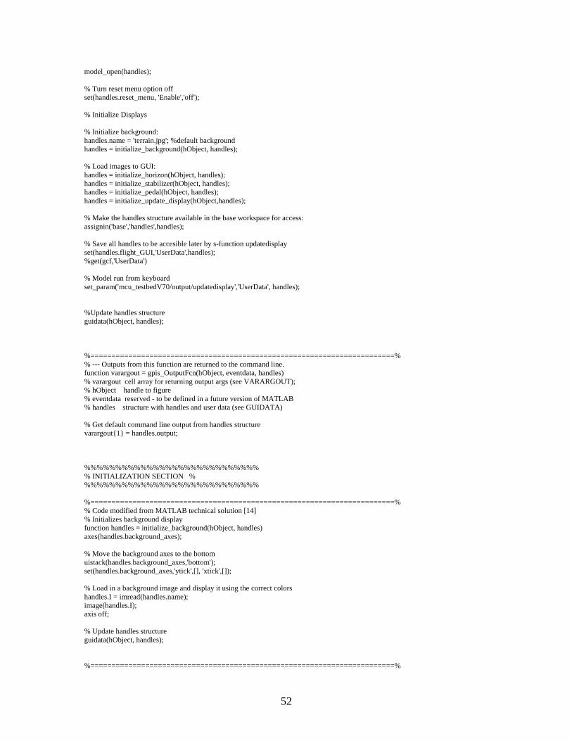
model_open(handles); % Turn reset menu option off set(handles.reset_menu, 'Enable','off'); % Initialize Displays % Initialize background: handles.name = 'terrain.jpg'; %default background handles = initialize_background(hObject, handles); % Load images to GUI: handles = initialize_horizon(hObject, handles); handles = initialize_stabilizer(hObject, handles); handles = initialize_pedal(hObject, handles); handles = initialize_update_display(hObject,handles); % Make the handles structure available in the base workspace for access: assignin('base','handles',handles); % Save all handles to be accesible later by s-function updatedisplay set(handles.flight_GUI,'UserData',handles); %get(gcf,'UserData') % Model run from keyboard set_param('mcu_testbedV70/output/updatedisplay','UserData', handles); %Update handles structure guidata(hObject, handles); %========================================================================% % --- Outputs from this function are returned to the command line. function varargout = gpis_OutputFcn(hObject, eventdata, handles) % varargout cell array for returning output args (see VARARGOUT); % hObject handle to figure % eventdata reserved - to be defined in a future version of MATLAB % handles structure with handles and user data (see GUIDATA) % Get default command line output from handles structure varargout{1} = handles.output; %%%%%%%%%%%%%%%%%%%%%%%%%%%% % INITIALIZATION SECTION % %%%%%%%%%%%%%%%%%%%%%%%%%%%% %========================================================================% % Code modified from MATLAB technical solution [14] % Initializes background display function handles = initialize_background(hObject, handles) axes(handles.background_axes); % Move the background axes to the bottom uistack(handles.background_axes,'bottom'); set(handles.background_axes,'ytick',[], 'xtick',[]); % Load in a background image and display it using the correct colors handles.I = imread(handles.name); image(handles.I); axis off; % Update handles structure guidata(hObject, handles); %========================================================================%

52

% Create attitude indicator display function handles = initialize_horizon(hObject, handles) axes(handles.horizon_axes); set(handles.horizon_axes,'visible','off'); image(imread('attitude_indicator.bmp')); % Remove tickmarks and labels that are inserted when using IMAGE: set(handles.horizon_axes,'ytick',[],'xtick',[],'ydir', 'normal'); hold on; % Plotting the initial position of the aircraft figure: handles.line(1) = plot([65 135], [100 100], 'r','LineWidth',[3]); %main handles.line(2) = plot([100 100], [85 115], 'r', 'LineWidth',[3]);%center handles.line(3) = plot([55 65], [95 100], 'r', 'LineWidth',[3]);%leftedge handles.line(4) = plot([135 145], [100 95], 'r', 'LineWidth',[3]);%rightedge hold off; % Initialize value to be used in rotation computations later: set(handles.line(1),'UserData',0); % Create hgtransform object: handles.transform = hgtransform('Parent',handles.horizon_axes); set(handles.line,'Parent',handles.transform); % Update handles structure guidata(hObject, handles); %========================================================================% % Create stabilizer display function handles = initialize_stabilizer(hObject, handles) axes(handles.stabilizer_axes); set(handles.stabilizer_axes,'Visible','off'); image(imread('stabilizer.bmp')); % Remove tickmarks and labels that are inserted when using IMAGE: set(handles.stabilizer_axes,'ytick',[],'xtick',[]); hold on; %Plotting the initial position of the stabilizer: handles.stabilizer_line = plot([6 14], [18.75 18.75], 'g', 'EraseMode', 'xor','LineWidth',[1.5]); hold off; % Variable for record keeping: handles.stabilizer_prev_value = 0; % Update handles structure guidata(hObject, handles); %========================================================================% % Create pedal display function handles = initialize_pedal(hObject, handles) axes(handles.pedal_axes); set(handles.pedal_axes,'Visible','off'); image(imread('pedal.bmp')); % Remove tickmarks and labels that are inserted when using IMAGE: set(handles.pedal_axes,'ytick',[],'xtick',[]); hold on; %Plotting the initial position of the pedal: handles.pedal_line = plot([68 68], [32 46], 'g', 'EraseMode', 'xor','LineWidth',[2]); hold off; % Variable for record keeping: handles.pedal_prev_value = 0; % Update handles structure guidata(hObject, handles);

53

%========================================================================% % Routine to set GUI to trim values; function handles = initialize_update_display(hObject, handles) % Variable to check setup was executed: ok = evalin('base','setup_ok'); if ok handles.u0 = evalin('base','u0'); % u0 = [dl_stab dl_w dl_p dl_c dl_sbh NaN dl_fh gear] handles.Tn0 =evalin('base','Tn0'); % Tn0 = [Tn1 Tn2 Tn3 Tn4] values for the four thrust engines handles.x0 = evalin('base','x0'); % x0 = [p q r Vtas alpha beta phi theta psi he xe ye]; handles.throttle_value = handles.Tn0(1); % Initial values for display set(handles.pedal_edit,'String', num2str(round(rad2deg(handles.u0(3))))); set(handles.column_edit,'String', num2str(round(rad2deg(handles.u0(4))))); set(handles.column_slider,'Value', rad2deg(handles.u0(4))); set(handles.stabilizer_edit,'String', num2str(round(rad2deg(handles.u0(1))))); set(handles.wheel_edit,'String', num2str(round(rad2deg(handles.u0(2))))); set(handles.wheel_slider,'Value', rad2deg(handles.u0(2))); set(handles.throttle_edit,'String', num2str(round(100 * (handles.throttle_value / 222400)))); set(handles.throttle_slider,'Value', round(100 * (handles.throttle_value / 222400))); set(handles.show_height_text,'String', num2str(round(handles.x0(10)))); set(handles.show_vtas_text,'String', num2str(round(handles.x0(4)))); set(handles.show_yaw_angle_text,'String', num2str(round(rad2deg(handles.x0(9))))); % Update display images: % Update stabilizer animation: axes(handles.stabilizer_axes); hold on; stabilizer_y = 18.75 + (round(rad2deg(handles.u0(1))) * 10.1); set(handles.stabilizer_line,'YData',[stabilizer_y, stabilizer_y]); drawnow; hold off; % Update pedal animation: axes(handles.pedal_axes); hold on; pedal_x = 68 + (round(rad2deg(handles.u0(3))) * 3.3); set(handles.pedal_line,'XData',[pedal_x, pedal_x]); drawnow; hold off; % Update aircraft figure: axes(handles.horizon_axes); hold on; % Height adjustment: % Pitch angle: anglep = rad2deg(handles.x0(8)); % Translate takes you directly to pitch angle desired. pitch = makehgtform('translate',[0 anglep 0]); set(handles.transform,'Matrix',pitch); % Bank adjustment: % Roll angle: if handles.reset == 1 rotation_angle = get(handles.line(1),'UserData'); % Turn reset flag off: handles.reset = 0;

54

else rotation_angle = 0; end angle_roll = rad2deg(handles.x0(7)); center = [100 100 0]; zdir = [0 0 1]; if rotation_angle > angle_roll angle = - abs(rotation_angle - angle_roll); if angle_roll < 0 rotate(handles.line,zdir,-angle, center); else rotate(handles.line,zdir,-angle, center); end set(handles.line(1),'UserData', (rotation_angle + angle)); elseif rotation_angle < angle_roll angle = abs(angle_roll - rotation_angle); if angle_roll < 0 rotate(handles.line,zdir,angle, center); else rotate(handles.line,zdir,-angle, center); end set(handles.line(1),'UserData', (rotation_angle + angle)); else angle = 0; rotate(handles.line,zdir,angle, center); set(handles.line(1),'UserData',rotation_angle); end hold off; % Update pilot variable for model: handles.pilot = [handles.u0(4) handles.u0(2) handles.u0(3) handles.u0(1)... handles.Tn0(1) handles.Tn0(2) handles.Tn0(3) handles.Tn0(4)]; assignin('base','pilot',handles.pilot); % pilot = [ column wheel pedal stabilizer thrust1 thrust2 thrust3 trust4] % Update handles structure guidata(hObject, handles); else errordlg('Initialization error. Restart application', 'GPIS Initialization Error'); end %%%%%%%%%%%%%%%%%%%%%%%%%%%%% % SLIDER/EDIT BOX SECTION % %%%%%%%%%%%%%%%%%%%%%%%%%%%%% %========================================================================% % --- Executes during object creation, after setting all properties. function pedal_edit_CreateFcn(hObject, eventdata, handles) % hObject handle to pedal_edit (see GCBO) % eventdata reserved - to be defined in a future version of MATLAB % handles empty - handles not created until after all CreateFcns called if ispc set(hObject,'BackgroundColor','white'); else set(hObject,'BackgroundColor',get(0,'defaultUicontrolBackgroundColor')); end %========================================================================% function pedal_edit_Callback(hObject, eventdata, handles) % hObject handle to pedal_edit (see GCBO)

55

% eventdata reserved - to be defined in a future version of MATLAB % handles structure with handles and user data (see GUIDATA) % Ensure model is open model_open(handles); disp_pedal = str2double(get(handles.pedal_edit,'String')); % Get range information stored in user data: deflection_range = get(handles.pedal_edit,'UserData'); % Determine whether disp_pedal is a number between -13 and 13 if isnumeric(disp_pedal) & ... disp_pedal >= deflection_range(1) & ... disp_pedal <= deflection_range(2) set(hObject,'String', disp_pedal); % Update stabilizer animation: axes(handles.pedal_axes); hold on; pedal_x = 68 + (disp_pedal * 3.3); set(handles.pedal_line,'XData',[pedal_x, pedal_x]); drawnow; hold off; % Store changed attribute handles.pilot(3) = deg2rad(-disp_pedal); assignin('base','pilot',handles.pilot); handles.pedal_prev_value = disp_pedal; guidata(hObject,handles); % store the changes else % Display previous value guidata(hObject,handles); % store the changes set(handles.pedal_edit,'String', handles.pedal_prev_value); end %========================================================================% % --- Executes during object creation, after setting all properties. function wheel_edit_CreateFcn(hObject, eventdata, handles) % hObject handle to wheel_edit (see GCBO) % eventdata reserved - to be defined in a future version of MATLAB % handles empty - handles not created until after all CreateFcns called if ispc set(hObject,'BackgroundColor','white'); else set(hObject,'BackgroundColor',get(0,'defaultUicontrolBackgroundColor')); end %========================================================================% function wheel_edit_Callback(hObject, eventdata, handles) % hObject handle to wheel_edit (see GCBO) % eventdata reserved - to be defined in a future version of MATLAB % handles structure with handles and user data (see GUIDATA) % Ensure model is open model_open(handles); disp_wheel= str2double(get(handles.wheel_edit,'String')); % Determine whether disp_wheelis a number between -88 and 88 if isnumeric(disp_wheel) & ... disp_wheel >= get(handles.wheel_slider,'Min') & ... disp_wheel <= get(handles.wheel_slider,'Max') set(hObject,'String', disp_wheel); set(handles.wheel_slider,'Value',disp_wheel);

56

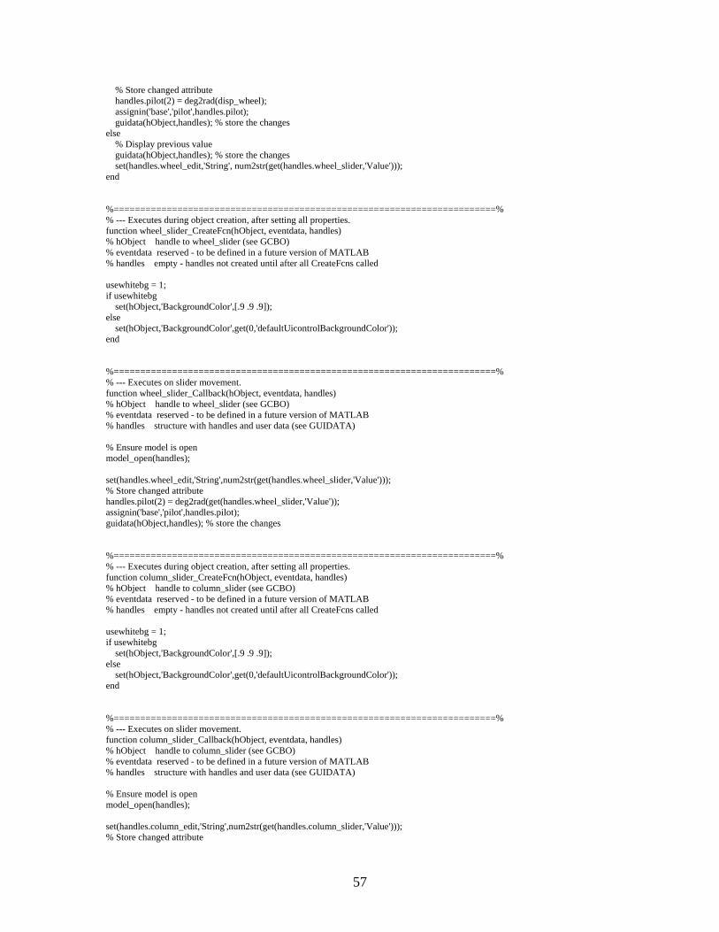
% Store changed attribute handles.pilot(2) = deg2rad(disp_wheel); assignin('base','pilot',handles.pilot); guidata(hObject,handles); % store the changes else % Display previous value guidata(hObject,handles); % store the changes set(handles.wheel_edit,'String', num2str(get(handles.wheel_slider,'Value'))); end %========================================================================% % --- Executes during object creation, after setting all properties. function wheel_slider_CreateFcn(hObject, eventdata, handles) % hObject handle to wheel_slider (see GCBO) % eventdata reserved - to be defined in a future version of MATLAB % handles empty - handles not created until after all CreateFcns called usewhitebg = 1; if usewhitebg set(hObject,'BackgroundColor',[.9 .9 .9]); else set(hObject,'BackgroundColor',get(0,'defaultUicontrolBackgroundColor')); end %========================================================================% % --- Executes on slider movement. function wheel_slider_Callback(hObject, eventdata, handles) % hObject handle to wheel_slider (see GCBO) % eventdata reserved - to be defined in a future version of MATLAB % handles structure with handles and user data (see GUIDATA) % Ensure model is open model_open(handles); set(handles.wheel_edit,'String',num2str(get(handles.wheel_slider,'Value'))); % Store changed attribute handles.pilot(2) = deg2rad(get(handles.wheel_slider,'Value')); assignin('base','pilot',handles.pilot); guidata(hObject,handles); % store the changes %========================================================================% % --- Executes during object creation, after setting all properties. function column_slider_CreateFcn(hObject, eventdata, handles) % hObject handle to column_slider (see GCBO) % eventdata reserved - to be defined in a future version of MATLAB % handles empty - handles not created until after all CreateFcns called usewhitebg = 1; if usewhitebg set(hObject,'BackgroundColor',[.9 .9 .9]); else set(hObject,'BackgroundColor',get(0,'defaultUicontrolBackgroundColor')); end %========================================================================% % --- Executes on slider movement. function column_slider_Callback(hObject, eventdata, handles) % hObject handle to column_slider (see GCBO) % eventdata reserved - to be defined in a future version of MATLAB % handles structure with handles and user data (see GUIDATA) % Ensure model is open model_open(handles); set(handles.column_edit,'String',num2str(get(handles.column_slider,'Value'))); % Store changed attribute

57

handles.pilot(1) = deg2rad(get(handles.column_slider,'Value')); assignin('base','pilot',handles.pilot); guidata(hObject,handles); % store the changes %========================================================================% % --- Executes during object creation, after setting all properties. function column_edit_CreateFcn(hObject, eventdata, handles) % hObject handle to column_edit (see GCBO) % eventdata reserved - to be defined in a future version of MATLAB % handles empty - handles not created until after all CreateFcns called if ispc set(hObject,'BackgroundColor','white'); else set(hObject,'BackgroundColor',get(0,'defaultUicontrolBackgroundColor')); end %========================================================================% function column_edit_Callback(hObject, eventdata, handles) % hObject handle to column_edit (see GCBO) % eventdata reserved - to be defined in a future version of MATLAB % handles structure with handles and user data (see GUIDATA) % Ensure model is open model_open(handles); disp_column = str2double(get(handles.column_edit,'String')); % Determine whether disp_column is a number between -12 and 12 if isnumeric(disp_column) & ... disp_column >= get(handles.column_slider,'Min') & ... disp_column <= get(handles.column_slider,'Max') set(hObject,'String', disp_column); set(handles.column_slider,'Value',disp_column); % Store changed attribute handles.pilot(1) = deg2rad(disp_column); assignin('base','pilot',handles.pilot); guidata(hObject,handles); % store the changes else % Display previous value guidata(hObject,handles); % store the changes set(handles.column_edit,'String',num2str(get(handles.column_slider,'Value'))); end %========================================================================% % --- Executes during object creation, after setting all properties. function throttle_slider_CreateFcn(hObject, eventdata, handles) % hObject handle to throttle_slider (see GCBO) % eventdata reserved - to be defined in a future version of MATLAB % handles empty - handles not created until after all CreateFcns called % Hint: slider controls usually have a light gray background, change % 'usewhitebg' to 0 to use default. See ISPC and COMPUTER. usewhitebg = 1; if usewhitebg set(hObject,'BackgroundColor',[.9 .9 .9]); else set(hObject,'BackgroundColor',get(0,'defaultUicontrolBackgroundColor')); end %========================================================================% % --- Executes on slider movement. function throttle_slider_Callback(hObject, eventdata, handles) % hObject handle to throttle_slider (see GCBO) % eventdata reserved - to be defined in a future version of MATLAB % handles structure with handles and user data (see GUIDATA)

58

% Ensure model is open model_open(handles); set(handles.throttle_edit,'String',num2str(get(handles.throttle_slider,'Value'))); %Value of thrust in Newtons handles.throttle_value = ((get(handles.throttle_slider,'Value')) / 100 ) * 222400; % Store changed attribute handles.pilot(5:8) = handles.throttle_value; %replicate value to all Tn positions assignin('base','pilot',handles.pilot); guidata(hObject,handles); % store the changes %========================================================================% % --- Executes during object creation, after setting all properties. function throttle_edit_CreateFcn(hObject, eventdata, handles) % hObject handle to throttle_edit (see GCBO) % eventdata reserved - to be defined in a future version of MATLAB % handles empty - handles not created until after all CreateFcns called if ispc set(hObject,'BackgroundColor','white'); else set(hObject,'BackgroundColor',get(0,'defaultUicontrolBackgroundColor')); end %========================================================================% function throttle_edit_Callback(hObject, eventdata, handles) % hObject handle to throttle_edit (see GCBO) % eventdata reserved - to be defined in a future version of MATLAB % handles structure with handles and user data (see GUIDATA) % Ensure model is open model_open(handles); disp_throttle = str2double(get(handles.throttle_edit,'String')); % Determine whether disp_throttle is a number from 0 to 100 percent if isnumeric(disp_throttle) & ... disp_throttle >= get(handles.throttle_slider,'Min') & ... disp_throttle <= get(handles.throttle_slider,'Max') set(hObject,'String', disp_throttle); set(handles.throttle_slider,'Value',disp_throttle); %Value of thrust in Newtons handles.throttle_value = (disp_throttle / 100 ) * 222400; % Store changed attribute handles.pilot(5:8) = handles.throttle_value; assignin('base','pilot',handles.pilot); guidata(hObject,handles); % store the changes else % Display previous value guidata(hObject,handles); % store the changes set(handles.throttle_edit,'String',num2str(get(handles.throttle_slider,'Value'))); end %========================================================================% % --- Executes during object creation, after setting all properties. function stabilizer_edit_CreateFcn(hObject, eventdata, handles) % hObject handle to stabilizer_edit (see GCBO) % eventdata reserved - to be defined in a future version of MATLAB % handles empty - handles not created until after all CreateFcns called if ispc set(hObject,'BackgroundColor','white'); else set(hObject,'BackgroundColor',get(0,'defaultUicontrolBackgroundColor')); end

59

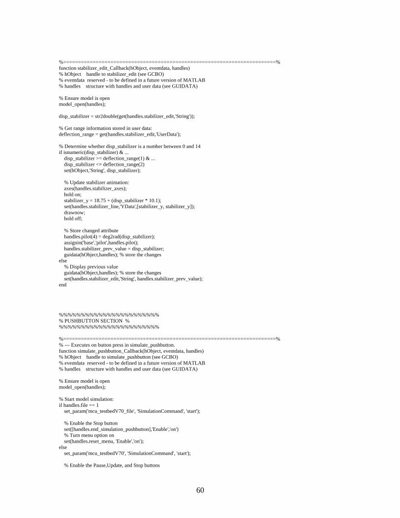
%========================================================================% function stabilizer_edit_Callback(hObject, eventdata, handles) % hObject handle to stabilizer_edit (see GCBO) % eventdata reserved - to be defined in a future version of MATLAB % handles structure with handles and user data (see GUIDATA) % Ensure model is open model_open(handles); disp_stabilizer = str2double(get(handles.stabilizer_edit,'String')); % Get range information stored in user data: deflection_range = get(handles.stabilizer_edit,'UserData'); % Determine whether disp_stabilizer is a number between 0 and 14 if isnumeric(disp_stabilizer) & ... disp_stabilizer >= deflection_range(1) & ... disp_stabilizer <= deflection_range(2) set(hObject,'String', disp_stabilizer); % Update stabilizer animation: axes(handles.stabilizer_axes); hold on; stabilizer_y = 18.75 + (disp_stabilizer * 10.1); set(handles.stabilizer_line,'YData',[stabilizer_y, stabilizer_y]); drawnow; hold off; % Store changed attribute handles.pilot(4) = deg2rad(disp_stabilizer); assignin('base','pilot',handles.pilot); handles.stabilizer_prev_value = disp_stabilizer; guidata(hObject,handles); % store the changes else % Display previous value guidata(hObject,handles); % store the changes set(handles.stabilizer_edit,'String', handles.stabilizer_prev_value); end %%%%%%%%%%%%%%%%%%%%%%% % PUSHBUTTON SECTION % %%%%%%%%%%%%%%%%%%%%%%% %========================================================================% % --- Executes on button press in simulate_pushbutton. function simulate_pushbutton_Callback(hObject, eventdata, handles) % hObject handle to simulate_pushbutton (see GCBO) % eventdata reserved - to be defined in a future version of MATLAB % handles structure with handles and user data (see GUIDATA) % Ensure model is open model_open(handles); % Start model simulation: if handles.file == 1 set_param('mcu_testbedV70_file', 'SimulationCommand', 'start'); % Enable the Stop button set([handles.end_simulation_pushbutton],'Enable','on') % Turn menu option on set(handles.reset_menu, 'Enable','on'); else set_param('mcu_testbedV70', 'SimulationCommand', 'start'); % Enable the Pause,Update, and Stop buttons

60

set([handles.pause_pushbutton,handles.update_pushbutton,handles.end_simulation_pushbutton],'Enable','on') % Turn menu option on set(handles.reset_menu, 'Enable','on'); end guidata(hObject,handles); % store the changes %========================================================================% % --- Executes on button press in pause_pushbutton. function pause_pushbutton_Callback(hObject, eventdata, handles) % hObject handle to pause_pushbutton (see GCBO) % eventdata reserved - to be defined in a future version of MATLAB % handles structure with handles and user data (see GUIDATA) set_param('mcu_testbedV70', 'SimulationCommand', 'pause'); set_param('mcu_testbedV70', 'SimulationCommand', 'pause'); set_param('mcu_testbedV70', 'SimulationCommand', 'pause'); %========================================================================% % --- Executes on button press in update_pushbutton. function update_pushbutton_Callback(hObject, eventdata, handles) % hObject handle to update_pushbutton (see GCBO) % eventdata reserved - to be defined in a future version of MATLAB % handles structure with handles and user data (see GUIDATA) %Check status of simulation: status = get_param('mcu_testbedV70', 'SimulationStatus'); if strcmp(status,'paused') set_param('mcu_testbedV70', 'SimulationCommand', 'update'); set_param('mcu_testbedV70', 'SimulationCommand', 'continue'); elseif strcmp(status,'stopped') set_param('mcu_testbedV70', 'SimulationCommand', 'update'); set_param('mcu_testbedV70', 'SimulationCommand', 'continue'); else errordlg('Simulation must be paused first.', 'Simulation Run Error'); end %========================================================================% % --- Executes on button press in end_simulation_pushbutton. function end_simulation_pushbutton_Callback(hObject, eventdata, handles) % hObject handle to end_simulation_pushbutton (see GCBO) % eventdata reserved - to be defined in a future version of MATLAB % handles structure with handles and user data (see GUIDATA) % End simulation: if handles.file == 1 set_param('mcu_testbedV70_file', 'SimulationCommand', 'stop'); set_param('mcu_testbedV70_file', 'SimulationCommand', 'stop'); set_param('mcu_testbedV70_file', 'SimulationCommand', 'stop'); else set_param('mcu_testbedV70', 'SimulationCommand', 'stop'); set_param('mcu_testbedV70', 'SimulationCommand', 'stop'); set_param('mcu_testbedV70', 'SimulationCommand', 'stop'); end %Parameters sent to base workspace: % x, xobs, xdotobs, yobs, yacc, deltas, y, u, ut, uctrl, Tn, uact_surf, uact_eng, % ref. The last three are not important. % Variables of interest in base workspace are: % - uctrl control surface deflection in degrees % - xobs variations in displacement(height, speed),airplane body angles (roll, pitch, yaw) % - Tn engine thrust variations uctrl = evalin('base','uctrl');

61

xobs = evalin('base','xobs'); Tn = evalin('base','Tn'); t = evalin('base','t'); vars = ['uctrl';'xobs ';'Tn ';'t ']; filename = 'outputs'; uisave(vars,filename); guidata(hObject, handles); % store changes % Turn reset button on set(handles.reset_pushbutton, 'Visible','on'); % Disable the Pause,Update, and Stop buttons set([handles.pause_pushbutton,handles.update_pushbutton,handles.end_simulation_pushbutton],'Enable','off') %========================================================================% % --- Executes on button press in reset_pushbutton. function reset_pushbutton_Callback(hObject, eventdata, handles) % hObject handle to reset_pushbutton (see GCBO) % eventdata reserved - to be defined in a future version of MATLAB % handles structure with handles and user data (see GUIDATA) % Reset button triggered: handles.reset = 1; % Update handles structure guidata(hObject, handles); % Update display to starting point: handles = initialize_update_display(hObject, handles); %handles = initialize_background(hObject, handles); % Turn button off set(handles.reset_pushbutton, 'Visible','off'); % Turn reset menu off set(handles.reset_menu, 'Enable','off'); % Update handles structure guidata(hObject, handles); %========================================================================% % --- Executes on button press in help_button. function help_button_Callback(hObject, eventdata, handles) % hObject handle to help_button (see GCBO) % eventdata reserved - to be defined in a future version of MATLAB % handles structure with handles and user data (see GUIDATA) path = which('B747SimpleHowTo.pdf'); open(path); %========================================================================% % --- Executes on button press in close_button. function close_button_Callback(hObject, eventdata, handles) % hObject handle to close_button (see GCBO) % eventdata reserved - to be defined in a future version of MATLAB % handles structure with handles and user data (see GUIDATA) selection = questdlg(['Are you sure you want to exit ' get(handles.output,'Name') '?'],... ['Confirm Close'],'Yes','No','Yes'); if strcmp(selection,'No') return; end close(handles.output); if handles.file == 1

62

close_system('mcu_testbedV70_file',0); else close_system('mcu_testbedV70',0); end clear all; %%%%%%%%%%%%%%%%%%%%%%% % MENU SECTION % %%%%%%%%%%%%%%%%%%%%%%% %========================================================================% function file_menu_Callback(hObject, eventdata, handles) % hObject handle to file_menu (see GCBO) % eventdata reserved - to be defined in a future version of MATLAB % handles structure with handles and user data (see GUIDATA) %========================================================================% function reset_menu_Callback(hObject, eventdata, handles) % hObject handle to reset_menu (see GCBO) % eventdata reserved - to be defined in a future version of MATLAB % handles structure with handles and user data (see GUIDATA) % Reset triggered: handles.reset = 1; % Update handles structure guidata(hObject, handles); % Update display to starting point: handles = initialize_update_display(hObject, handles); %handles = initialize_background(hObject, handles); % Turn menu option off set(handles.reset_menu, 'Enable','off'); % Turn button off set(handles.reset_pushbutton, 'Visible','off'); % Update handles structure guidata(hObject, handles); %========================================================================% function setup_menu_Callback(hObject, eventdata, handles) % hObject handle to load_menu (see GCBO) % eventdata reserved - to be defined in a future version of MATLAB % handles structure with handles and user data (see GUIDATA) % Restart process: setup; %========================================================================% function background_menu_Callback(hObject, eventdata, handles) % hObject handle to Untitled_1 (see GCBO) % eventdata reserved - to be defined in a future version of MATLAB % handles structure with handles and user data (see GUIDATA) selection = questdlg('Background display desired:', 'Background Selection', 'Cockpit','Sky','Terrain','Terrain'); switch selection case 'Cockpit' handles.name = 'cockpit.jpg'; initialize_background(hObject, handles); case 'Sky' handles.name = 'sky.jpg'; initialize_background(hObject, handles);

63

case 'Terrain' handles.name = 'terrain.jpg'; initialize_background(hObject, handles); end %end switch %========================================================================% function save_menu_Callback(hObject, eventdata, handles) % hObject handle to save_menu (see GCBO) % eventdata reserved - to be defined in a future version of MATLAB % handles structure with handles and user data (see GUIDATA) %Parameters sent to base workspace: % x, xobs, xdotobs, yobs, yacc, deltas, y, u, ut, uctrl, Tn, uact_surf, uact_eng, % ref. The last three are not important. % Variables of interest in base workspace are: % - uctrl control surface deflection in degrees % - xobs variations in displacement(height, speed),airplane body angles (roll, pitch, yaw) % - Tn engine thrust variations uctrl = evalin('base','uctrl'); xobs = evalin('base','xobs'); Tn = evalin('base','Tn'); t = evalin('base','t'); vars = ['uctrl';'xobs ';'Tn ';'t ']; filename = 'outputs'; uisave(vars,filename); guidata(hObject, handles); %========================================================================% function print_menu_Callback(hObject, eventdata, handles) % hObject handle to print_menu (see GCBO) % eventdata reserved - to be defined in a future version of MATLAB % handles structure with handles and user data (see GUIDATA) printdlg(handles.output) %========================================================================% function print_setup_menu_Callback(hObject, eventdata, handles) % hObject handle to print_setup_menu (see GCBO) % eventdata reserved - to be defined in a future version of MATLAB % handles structure with handles and user data (see GUIDATA) printdlg('-setup',handles.output) %========================================================================% function close_menu_Callback(hObject, eventdata, handles) % hObject handle to cloae_menu (see GCBO) % eventdata reserved - to be defined in a future version of MATLAB % handles structure with handles and user data (see GUIDATA) selection = questdlg(['Are you sure you want to exit ' get(handles.output,'Name') '?'],... ['Confirm Close'], 'Yes','No','Yes'); if strcmp(selection,'No') return; end close(handles.output); if handles.file == 1 close_system('mcu_testbedV70_file',0); else close_system('mcu_testbedV70',0); end clear all; %========================================================================% function help_menu_Callback(hObject, eventdata, handles)

64

% hObject handle to help_menu (see GCBO) % eventdata reserved - to be defined in a future version of MATLAB % handles structure with handles and user data (see GUIDATA) %========================================================================% function keyboard_menu_Callback(hObject, eventdata, handles) % hObject handle to keybozrd_menu (see GCBO) % eventdata reserved - to be defined in a future version of MATLAB % handles structure with handles and user data (see GUIDATA) % Assume file is in same directory path = which('keyboardinput.doc'); % Code modified from [15] word = actxserver('Word.Application'); set(word,'Visible',1); try invoke(word.Documents, 'Open', [path]); catch error('Cannot open file and/or file does not exist!'); end % end try %========================================================================% function manual_menu_Callback(hObject, eventdata, handles) % hObject handle to manual_menu (see GCBO) % eventdata reserved - to be defined in a future version of MATLAB % handles structure with handles and user data (see GUIDATA) % Assume file is in same directory path = which('usermanual.pdf'); open(path); %========================================================================% function about_menu_Callback(hObject, eventdata, handles) % hObject handle to about_menu (see GCBO) % eventdata reserved - to be defined in a future version of MATLAB % handles structure with handles and user data (see GUIDATA) about_GUI; %========================================================================% function exit_menu_Callback(hObject, eventdata, handles) % hObject handle to exit_menu (see GCBO) % eventdata reserved - to be defined in a future version of MATLAB % handles structure with handles and user data (see GUIDATA) selection = questdlg(['Are you sure you want to exit ' get(handles.output,'Name') '?'],... ['Confirm Close'], 'Yes','No','Yes'); if strcmp(selection,'No') return; end close(handles.flight_GUI); if handles.file == 1 close_system('mcu_testbedV70_file',0); else close_system('mcu_testbedV70',0); end clear all;

65

%%%%%%%%%%%%%%%%%%%%%%%%%%%%%%% % RADIOBUTTONS SECTION % %%%%%%%%%%%%%%%%%%%%%%%%%%%%%%% %========================================================================% % --- Executes on button press in keyboard_radiobutton. function keyboard_radiobutton_Callback(hObject, eventdata, handles) % hObject handle to keyboard_radiobutton (see GCBO) % eventdata reserved - to be defined in a future version of MATLAB % handles structure with handles and user data (see GUIDATA) % Check status of simulation: if handles.file == 1 status = get_param('mcu_testbedV70_file', 'SimulationStatus'); else status = get_param('mcu_testbedV70', 'SimulationStatus'); end if (status ~= 'stopped') if handles.file == 1 set_param('mcu_testbedV70_file', 'SimulationCommand', 'stop'); else set_param('mcu_testbedV70', 'SimulationCommand', 'stop'); end end if (get(hObject,'Value') == get(hObject,'Max'))% Radio button is selected % Ensure other radiobutton is off set(handles.file_radiobutton,'Value',0); set(handles.flight_GUI, 'KeyPressFcn','keypress'); handles.file = 0; % simulation controlled by keyboard % Ensure proper model is open model_open(handles); % Model run from keyboard set_param('mcu_testbedV70/output/updatedisplay','UserData', handles); guidata(hObject,handles); % store the changes % Warn user that simulation must be restarted: errordlg('Operation mode changed. Simulation must be restarted.', 'Operation Mode Changed'); end % Do nothing if radio button is not selected %========================================================================% % --- Executes on button press in file_radiobutton. function file_radiobutton_Callback(hObject, eventdata, handles) % hObject handle to file_radiobutton (see GCBO) % eventdata reserved - to be defined in a future version of MATLAB % handles structure with handles and user data (see GUIDATA) %Check status os simulation: status = get_param('mcu_testbedV70', 'SimulationStatus'); if (status ~= 'stopped') set_param('mcu_testbedV70', 'SimulationCommand', 'stop'); end if (get(hObject,'Value') == get(hObject,'Max'))% Radio button is selected % Ensure other radiobutton is off set(handles.keyboard_radiobutton,'Value',0); set(handles.flight_GUI, 'KeyPressFcn',[]); % File will run simulation: handles.file = 1;

66

[filename,pathname] = uigetfile('',' Select file to execute simulation:'); if isequal([filename,pathname],[0,0]) % Issue error dialog box: errordlg('No file was selected.', 'File Selection Error'); handles.file = 0; else file = fullfile(pathname,filename); % Must load variables called simrun and time load testing %load file; % NOTE: path must not contain blank spaces. % Variable to calculate time variables: %temp = length(simrun); % Final time to execute simulation: %tstop = temp * 0.2; % Create appropiate time variable to run file mode %time = (0 : (temp - 1))'; % Save loaded variable in base workspace to be accessed by Simulink assignin('base','simrun', simrun); assignin('base','time', time); %assignin('base','tstop', tstop); % Ensure proper model is open model_open(handles); % Model run from file set_param('mcu_testbedV70_file/output/updatedisplay','UserData', handles); % Warn user that simulation must be restarted: errordlg('Operation mode changed. Simulation must be restarted.', 'Operation Mode Changed'); end guidata(hObject,handles); % store the changes end % Do nothing if radio button is not selected

67

sfundisplay.m %%%%%%%%%%%%%%%%%%%%%%%%%%%%%%%%%%%%%%%%%%%%%%%%%%%%%%%%%%%%%%%%%%%%%%%%%%%%%%%%%%%%%%% % FUNCTION NAME: sfundisplay Coding started: 01/19/05 % Last revision: 08/24/05 % % PURPOSE: Update display. % % ACTIONS: Gets xobs and handles structure from base workspace. % Use parameters to update GUI. % % % REMARKS: Built from s-function template (Copyright 1990-2002 The MathWorks, Inc.) % Revision: 1.18 % Matlab 6.5 can be used. %%%%%%%%%%%%%%%%%%%%%%%%%%%%%%%%%%%%%%%%%%%%%%%%%%%%%%%%%%%%%%%%%%%%%%%%%%%%%%%%%%%%%%% function [sys,x0,str,ts] = sfundisplay(t,x,u,flag) switch flag, %%%%%%%%%%%%%%%%%% % Initialization % %%%%%%%%%%%%%%%%%% case 0, [sys,x0,str,ts]= mdlInitializeSizes; %%%%%%%%%% % Update % %%%%%%%%%% case 2, sys = mdlUpdate(t,x,u); %%%%%%%%%%%%%%%%%%% % Unhandled flags % %%%%%%%%%%%%%%%%%%% case { 1, 3, 4, 9 } % Don't do anything %%%%%%%%%%%%%%%%%%%% % Unexpected flags % %%%%%%%%%%%%%%%%%%%% otherwise error(['Unhandled flag = ',num2str(flag)]); end %%============================================================================= % mdlInitializeSizes % Return the sizes, initial conditions, and sample times for the S-function. %============================================================================= function [sys,x0,str,ts]=mdlInitializeSizes sizes = simsizes; sizes.NumContStates = 0; sizes.NumDiscStates = 0; sizes.NumOutputs = 0; sizes.NumInputs = 12;

68

sizes.DirFeedthrough = 1; sizes.NumSampleTimes = 1; % at least one sample time is needed sys = simsizes(sizes); % initialize the initial conditions x0 = []; % str is always an empty matrix str = []; % initialize the array of sample times ts = [0 0]; % end mdlInitializeSizes %============================================================================= % mdlUpdate % Handle discrete state updates, sample time hits, and major time step % requirements. %============================================================================= function sys=mdlUpdate(t,x,u) sys = []; xobs = [u(1) u(2) u(3) u(4) u(5) u(6) u(7) u(8) u(9) u(10) u(11) u(12)] ; % fig_handle is handle of figure where animation takes place: block_handle = gcb; handles = get_param(block_handle,'UserData'); fig_handles = handles.flight_GUI; % Check figure has been opened: if ~ishandle(fig_handles) gpis; end % Update display: handles.xobs = xobs; % xobs = [p q r Vtas alpha beta phi theta psi he xe ye]; disp_height = handles.xobs(10); if disp_height <= -1 % Don't forget that I is uint8 which is integer. You can convert it % to double by: crashed_I = double(handles.I); r = crashed_I(:,:,1); % red component r = (r + 1000); % you can increase by any number r = r * 255 / max(max(r)); % to scale between [0,255] % Add modified red component to image crashed_I(:,:,1) = r; image(uint8(crashed_I)); % convert back and display image % Log error message: errordlg('Aircraft crashed!', 'Simulation Ended'); % Stop simulation: set_param('mcu_testbedV70', 'SimulationCommand', 'stop'); % Disable the Pause,Update, and Stop buttons set([handles.pause_pushbutton,handles.update_pushbutton,handles.end_simulation_pushbutton],'Enable','off') % Turn reset button on set(handles.reset_pushbutton, 'Visible','on'); end % Values for display set(handles.show_height_text,'String', num2str(round(handles.xobs(10)))); set(handles.show_vtas_text,'String', num2str(round(handles.xobs(4)))); set(handles.show_yaw_angle_text,'String', num2str(round(rad2deg(handles.xobs(9))))); %Update display images:

69

%Update aircraft figure: axes(handles.horizon_axes); % Height adjustment: % Pitch angle: anglep = rad2deg(handles.xobs(8)); % Translate takes you directly to pitch angle desired. pitch = makehgtform('translate',[0 anglep 0]); set(handles.transform,'Matrix',pitch); % Bank adjustment: % Roll angle: angle_roll = rad2deg(handles.xobs(7)); % new rotation angle % previous rotation angle rotation_angle = get(handles.line(1),'UserData'); center = [100 100 0]; zdir = [0 0 1]; % axis about which we rotate if rotation_angle > angle_roll angle = - abs(rotation_angle - angle_roll); if angle_roll < 0 rotate(handles.line,zdir,-angle, center); else rotate(handles.line,zdir,-angle, center); end set(handles.line(1),'UserData', (rotation_angle + angle)); elseif rotation_angle < angle_roll angle = abs(angle_roll - rotation_angle); if angle_roll < 0 rotate(handles.line,zdir,angle, center); else rotate(handles.line,zdir,-angle, center); end set(handles.line(1),'UserData', (rotation_angle + angle)); else angle = 0; rotate(handles.line,zdir,angle, center); set(handles.line(1),'UserData',rotation_angle); end % end mdlUpdate

70

graph.m %%%%%%%%%%%%%%%%%%%%%%%%%%%%%%%%%%%%%%%%%%%%%%%%%%%%%%%%%%%%%%%%%%%%%%%%%%%%%%%%%%%%%%% % FUNCTION NAME: graph Coding started: 08/15/05 % Last revision: 08/20/05 % % PURPOSE: Graph outputs to a figure from a previously run simulation. % % KEY ACTIONS: The parameters that are graphed are: uctrl, Tn, and % xobs. They provide the most useful informational for % analysis. % % REMARKS: Code for this function extracted from FTLAB747. % Matlab 6.5 can be used. %%%%%%%%%%%%%%%%%%%%%%%%%%%%%%%%%%%%%%%%%%%%%%%%%%%%%%%%%%%%%%%%%%%%%%%%%%%%%%%%%%%%%%% % Create figure: figure() % Create subplot: subplot(221) plot(t,(180/pi)*uctrl(:,1:4)); title('Control Surfaces'); xlabel('time(sec)'), ylabel('deflection(degrees)'); legend('elevator','aileron','rudder','stablizer'); % Create subplot: subplot(222) plot(t,Tn); title('Engine Thrust'); xlabel('time(sec)'), ylabel('Thrust(N)'); legend('Eng 1','Eng 2','Eng 3', 'Eng 4'); % Create subplot: subplot(223) plot(t,(180/pi)*xobs(:,5:9)); title('Airplane Body Angles'); xlabel('time(sec)'), ylabel('angles(degrees)'); legend('attack ', 'sideslip', 'roll', 'pitch', 'yaw'); % Create subplot: subplot(224) plot(t, [xobs(:,4)/10 xobs(:,10)/100 xobs(:,11)/100 xobs(:,12)/10]) title('Variations in Linear Displacements'); xlabel('time(sec)'), ylabel('linear displacements'); legend('V_{TAS}/10','Height/100','x/100','y/10');

71

Appendix E Boeing 747 Information Appendix E included to provide general information on the performance capabilities of a Boeing 747 today. In addition, we have added a few images to help the user visualize the aircraft in question used for this research initiative. E.1 Cockpit Layout of Boeing 747

The following image is used to give the user a feel of what elements in the cockpit the

GPIS tool is meant to portray.

Figure E.1 Pilot control inputs in a Boeing 747 cockpit [30]

72

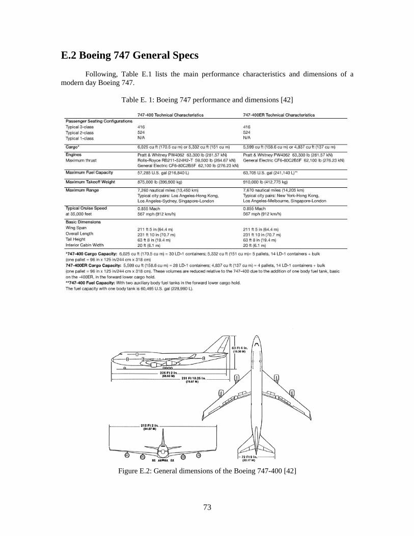
E.2 Boeing 747 General Specs

Following, Table E.1 lists the main performance characteristics and dimensions of a modern day Boeing 747.

Table E. 1: Boeing 747 performance and dimensions [42]

Figure E.2: General dimensions of the Boeing 747-400 [42]

73

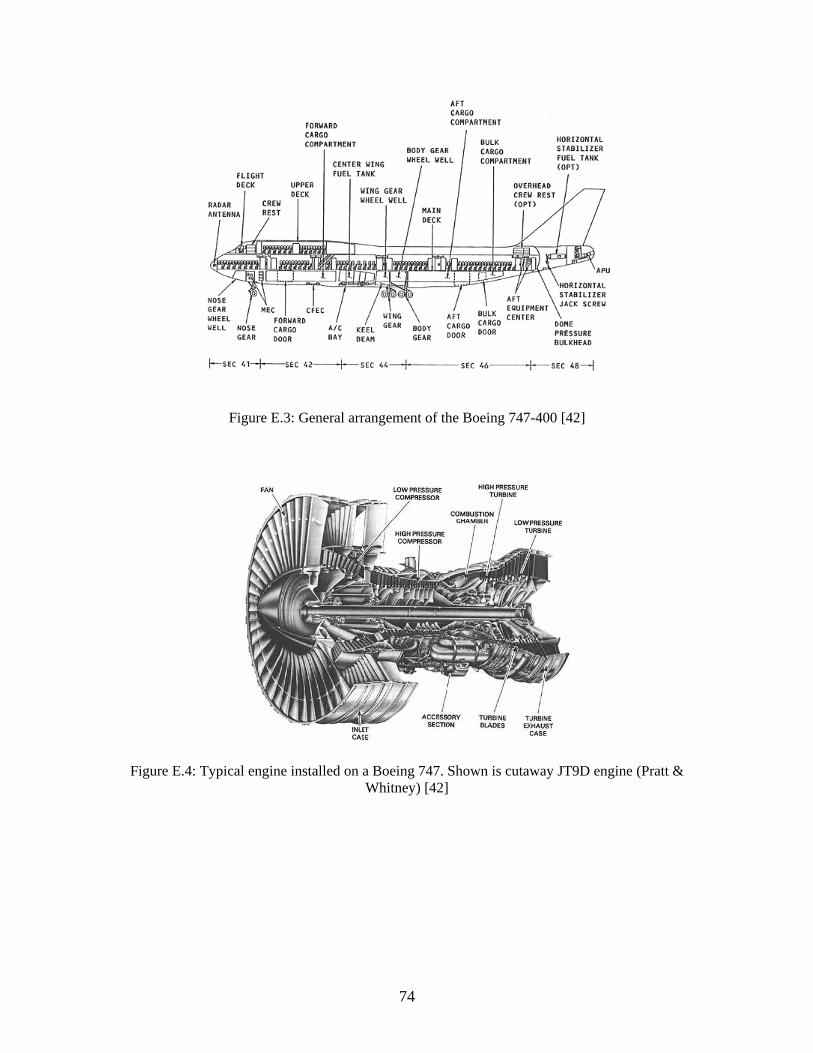
Figure E.3: General arrangement of the Boeing 747-400 [42]

Figure E.4: Typical engine installed on a Boeing 747. Shown is cutaway JT9D engine (Pratt & Whitney) [42]

74

VITA Jeffry Jorge Handal Bendeck was born on January 3, 1982, in Tegucigalpa, Honduras. Brother to three incredible kids, Jorge, Javier, and Joshua; son to two unbelievable parents, Rosemary and Jorge; and part of a great family, will be the first of generations to come to hold a master’s degree. During his graduate studies, Jeffry worked full time for the Office of Telecommunications at LSU, as an engineer. Additionally, he obtained a pilot’s license on September 9, 2004. His plans for the future include: keep working for LSU, obtain more advanced flight ratings, and further his education possibly in the business world. For now, he will remain a humble student until he receives the degree of Master of Science in Electrical Engineering for the Fall Commencement of 2005.

75