graphical models in speech and language...

Graphical Models in Speech and Language Research

Jeff A. BilmesUniversity of Washington

Department of EE, SSLI-Lab

Graphical ModelsJeff A. Bilmes@

Tutorial PhilosophyTutorial Philosophy• Questions?• Ideas?• Confusion?• Suggestions?• Please ask.


Detailed Outline1. Properties

a) Overview and Motivationb) GM Types and Constructsc) Theory and Practice of Dynamic GMsd) Explicit Temporal Structures

2. Specific Modelsa) GMs in Speechb) GMs in Languagec) GMs in Machine Translation

3. Toolkits4. Discussion/Open Questions


Cause and Effect• Fact: At least 196 cows died in Thailand,

Jan/Feb 2004, as have 16 people.• Consequence: Canadian officials in April

2004 killed 19 million birds in British Columbia (chickens, ducks, geese, etc.)

• Possible cause I: Original deaths due to avian influenza (H5N1 or bird flu)

• Possible cause II: They died of old age!


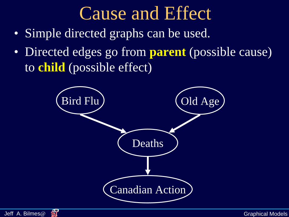
• Simple directed graphs can be used.• Directed edges go from parent (possible cause)

to child (possible effect)

Cause and Effect

Deaths

Bird Flu Old Age

Canadian Action


Cause and Effect

Computing Probabilities:

Deaths

Bird Flu Old Age

Canadian Action• Quantities of interest:

Examples:Pr( Deaths | Flu and Old )Pr( Deaths | Old ) Pr( Bird Flu | Canadian Action )

Examples:• In general, does old age increase the chance that a cow has contracted bird flu (if at all)?• If we know the action by Canada occurred, does having bird flu decrease the chance that it was old when it died?

AskingQuestions:

Very simple scenario, with obvious answers to questions. What happens with more complicated real-world problems?


Realistic Domains• Graph Represents relational structure of domain. • Regardless of graph complexity, same set of

algorithms used to compute desirable quantities and answer all questions.

• Example: Is Pr(A|B) larger or smaller than Pr(A|B,C)?

• Graphs are natural way to explain complex situations on an intuitive visual level.

• Graphs are used everywhere, for many different purposes. Here they have a specific meaning: Random variables and conditional independence.

B

C

A


Graphical Models (GMs)

• Structure• Algorithms• Language• Approximations• Data-Bases


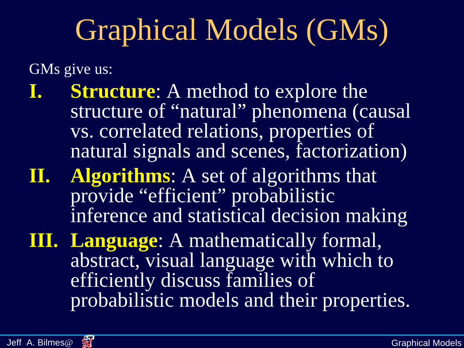
Graphical Models (GMs)GMs give us:I. Structure: A method to explore the

structure of “natural” phenomena (causal vs. correlated relations, properties of natural signals and scenes, factorization)

II. Algorithms: A set of algorithms that provide “efficient” probabilistic inference and statistical decision making

III. Language: A mathematically formal, abstract, visual language with which to efficiently discuss families of probabilistic models and their properties.


Graphical Models (GMs)GMs give us (cont):IV. Approximation: Methods to explore

systems of approximation and their implications. E.g., what are the consequences of a (perhaps known to be) wrong assumption?

V. Data-base: Provide a probabilistic “data-base” and corresponding “search algorithms” for making queries about properties in such model families.


Topology of Graphical ModelsGraphical Models

Chain GraphsCausal Models

DGMsUGMs

Bayesian Networks

MRFs

Gibbs/BoltzmanDistributions

DBNs Mixture Models

Decision Trees

Simple Models

PCA

LDAHMM

Factorial HMM/Mixed Memory Markov Models

BMMs

Kalman

Other Semantics

FST

Dependency Networks

Segment Models

AR

ZMs

Factor Graphs


A Pause For QuestionsA Pause For Questions• Questions?• Ideas?• Confusion?• Suggestions?• Please ask.


Outline1. Properties





Three Important Graph Types

• Three (of many) types of GM– Bayesian Networks– Undirected Graphical Models– Factor Graphs

• Each conveys a different family• Each type of graph conveys factorization of

probability distributions in some way.


Factorization and Conditional Independence

• Factorization of probability distributions usually (but not always) implies some form of conditional independence.

• Conditional Independence:

• Holds if and only if there are functions f() and g() such that:

|A B CX X X⊥⊥

( , , ) ( , ) ( , )A B C A C B Cp x x x g x x h x x=

Notation: XA is a set of random variable indexed by the set A. So if A =

{1,2,4}, then XA = {X1, X2, X4}


Bayesian Networks

Sub-family specification:Directed acyclic graph

(DAG)• Nodes - random variables • Edges - direct “influence”

Instantiation: Set of conditional probability distributions

0.9 0.1

e

be

0.2 0.8

0.01 0.99

0.9 0.1

bebb

e

BE P(A | E,B)Earthquake

Radio

Burglary

Alarm

Call

• Only one type of graphical model (many others exist)• Compact representation: factors of probabilities of

children given parents.

Together:Defines a unique distribution in a factored form

( , , , , ) ( ) ( ) ( | , ) ( | ) ( | )P B E A C R P B P E P A B E P R E P C A=


Bayesian Networks• When is ?• Only when C d-separates A from B, i.e. if:

for all paths from A to B, there is a v on the path that is blocked. Node v is blocked if either:

1. →v→ or ←v→ and v∈ C2. →v← and neither v nor any descendants are in C

• Equivalent to “directed local Markov property”– A variable is conditionally independent of its non-

descendants given its parents• See Lauritzen ’96 for other properties.• Distribution factors as product of conditional probability

distributions of child given its parents P(c|parents)

|A B CX X X⊥⊥


Three Basic Cases• Graphs encode conditional independence

via factorization.V1

V2 V3

2 3 1|V V V⊥⊥

V1

V2 V3

2 3V V¬⊥⊥2 3V V⊥⊥

2 3 1|V V V¬⊥⊥

V1

V2 V3

2 3 1|V V V⊥⊥

2 3V V¬⊥⊥


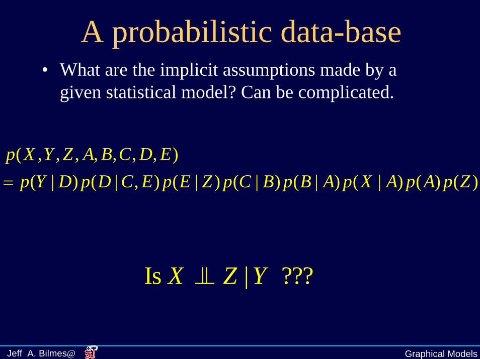
A probabilistic data-base• What are the implicit assumptions made by a

given statistical model? Can be complicated.

( , , , , , , , )( | ) ( | , ) ( | ) ( | ) ( | ) ( | ) ( ) ( )

p X Y Z A B C D Ep Y D p D C E p E Z p C B p B A p X A p A p Z=

Is | ???X Z Y⊥⊥


A probabilistic data-base• GMs can help illuminate the answer.

( , , , , , , , )( | ) ( | , ) ( | ) ( | ) ( | ) ( | ) ( ) ( )

p X Y Z A B C D Ep Y D p D C E p E Z p C B p B A p X A p A p Z=

Y

D

C E

B ZX

A| ???X Z Y⊥⊥

No!!


Hidden Variables• Hidden variables can introduce significant

capabilities for probabilistic queries (called inference).

ObservedObserved

∑=2

122313 )|()|()|(v

vvpvvpvvpV1 V2 V3

Hidden )|(),|( 23213 vvpvvvp =


Nodes as Inputs and/or Outputs

• Variables in a GM can be both an input or an output variable at different times (unlike a neural network). This can be very useful.

OutputInput

3 1( | )p v vV1 V2 V3

InputOutput

1 3( | )p v vV1 V2 V3


Undirected GMs (UGMs)• When is XA || XB | XC?• Only when C separates A from B. I.e., if:

for all paths from A to B, there is a v on the path s.t. v∈ C

• Simpler semantics than Bayesian networks.• Equivalent to “global Markov property”, plus

others (again see Lauritzen ‘96)


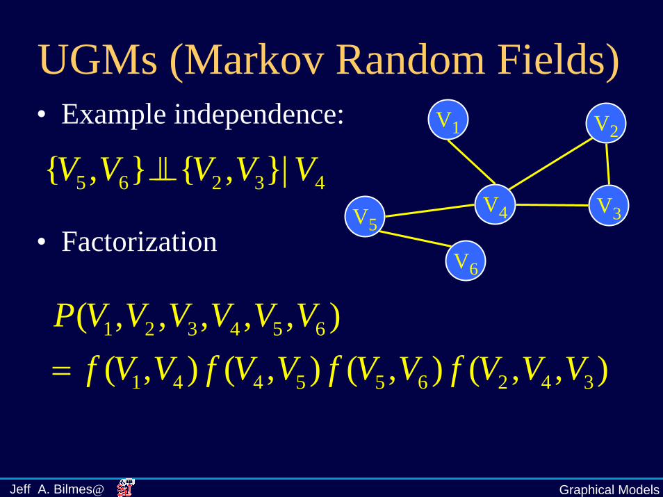
UGMs (Markov Random Fields)• Example independence:

• Factorization

V1 V2

V3V4V5

V6

5 6 2 3 4{ , } { , }|V V V V V⊥⊥

1 2 3 4 5 6

1 4 4 5 5 6 2 4 3

( , , , , , )( , ) ( , ) ( , ) ( , , )

P V V V V V Vf V V f V V f V V f V V V=


Example: Undirected GMs (UGMs)∏Ψ=

ccX X

ZXP

c)(1)(

)}(1exp{1

0

xUTkZ

−=

)()( cc

X xHxUc∑=

If Gibbs:

Semantics: Simple SeparationXA || XB | XC if XC separates XA from XB in graph.

c = cliques (completely connected nodes) in graph.

W X

Y ZCliques are: { (W,X), (X,Z), (Z,Y), (Y,W) }

UGMs are the same as MRFs


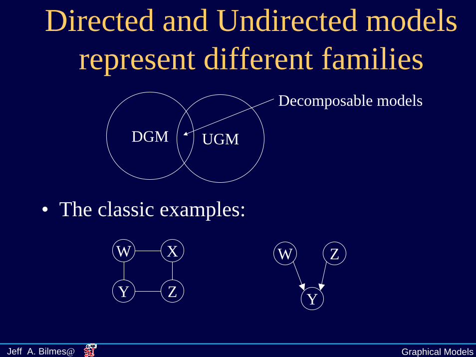
Directed and Undirected models represent different families

Decomposable models

DGM UGM

• The classic examples:

W X

Y Z

W

Y

Z


Factor Graphs• Graph represents all possible factorizations

of a distribution.• Simplest example:

1 2 3 1 2 2 3 3 1( , , ) ( , ) ( , ) ( , )P V V V f V V f V V f V V=V1

V2 V3


Dynamic Bayesian Networks(DBNs)

• Most appropriate for speech/language.• DBNs are Bayesian Networks over time• Specified using a “rolled up” template• In unrolled DBN, all variables sharing same

origin in template have tied parameters.• Allows for specifying graph over arbitrary

length series.


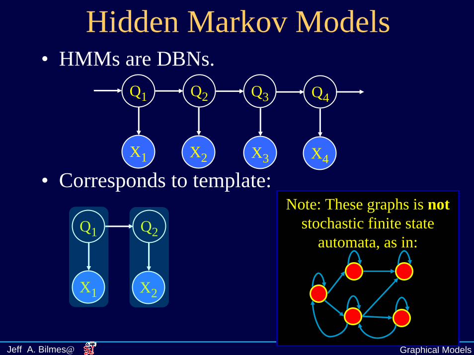
Hidden Markov Models

Q1 Q2 Q3 Q4

X1 X2 X3 X4

• HMMs are DBNs.

• Corresponds to template:

Q1 Q2

X1 X2

Note: These graphs is notstochastic finite state

automata, as in:


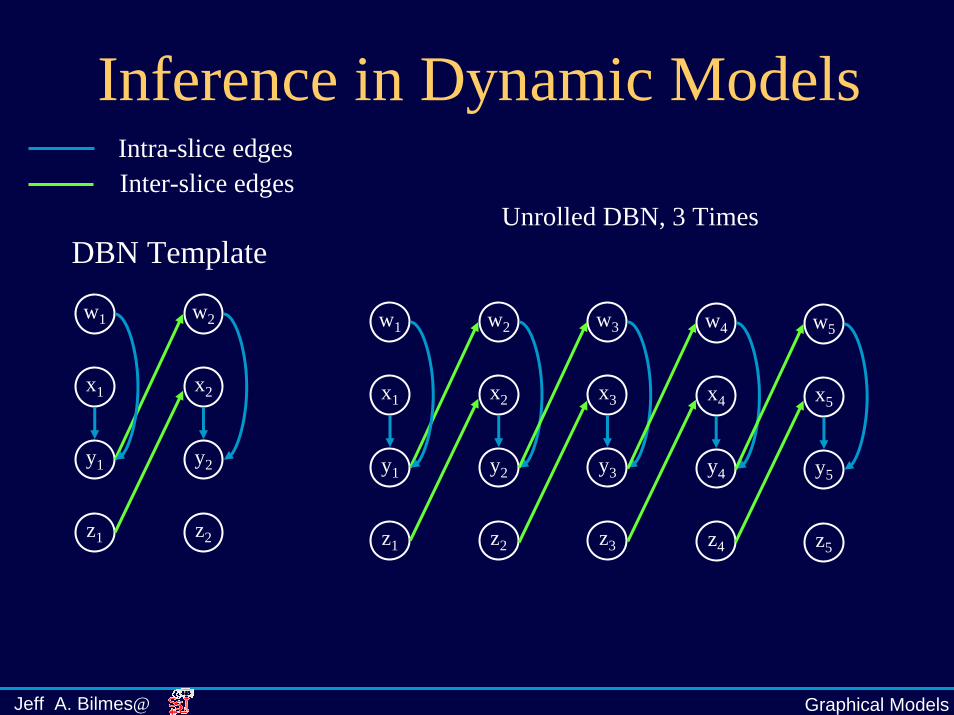
Dynamic Bayesian Networks• More generally, DBN specifies template to

be unrolled:Intra-slice edgesInter-slice edges Unrolled DBN, 3 Times

DBN Template


General Probabilistic Inference

X1

X3

X2

X5

X6

X4

)(),(5:2

6:161 ∑=x

xpxxP)(/),()|( 66161 xpxxpxxP =

Exploit local structure to provide for efficient inference O(r3) rather than O(r6)(variable elimination algorithm)

2:5

2:5

2 3 5 4

1 2 3 4 5 6

1 2 1 3 1 4 2 6 2 5 5 3

1 2 1 3 1 6 2 5 5 3 4 2

( , , , , , )

( ) ( | ) ( | ) ( | ) ( | , ) ( | )

( ) ( | ) ( | ) ( | , ) ( | ) ( | )

x

x

x x x x

P x x x x x x

P x P x x P x x P x x P x x x P x x

P x P x x P x x P x x x P x x P x x

=

=

∑

∑

∑ ∑ ∑ ∑

• Way in which sums are distributed into products corresponds to different ways of running the junction tree algorithm (generalization of Baum Welsh)


Moralization & Triangulation, lead to Junction Tree

B

A

CD

E F G

H I

B

A

CD

E F G

H I

B

A

CD

E F G

H I

A,B,C,D

B,C,D,F

B,E,F F,D,G

E,F,H F,G,I

Triangulated/Decomposable/Eliminatable

Original Moralized

Complexity of inference:

))((∑c

csO ||)( crcs ≈Junction Tree


Moralization & Triangulation• Moralization

– why ok? More edges, fewer independence assumptions, bigger family

– why needed? So UGM doesn’t violate BN semantics, summations include parents in cliques.

• Triangulation– why ok? Fewer independencies -> bigger family– why needed? To get a decomposable graph, where

junction tree (with running intersection property) exists and message passing algorithm is correct (i.e., local consistency implies global consistency)


Inference: Message Passing in JT

A,B,C,D

B,C,D,F

B,E,F F,D,G

E,F,H F,G,I

Select Root of JT

1. Collect Evidence Phase2. Distribute Evidence Phase

Now, All cliques equal the joint of their variables and any evidence (observations), e.g., P(A,B,C,D,Obs), P(B,C,D,F,Obs), etc.


Inference in Dynamic Models

• Inference procedures are equivalent to forming a “dynamic” Junction Tree

• Generalizes Forward/Backward (Baum/Welch) procedure in HMMs

• Dynamic Junction Tree is much wider than higher.


Inference in Dynamic ModelsIntra-slice edgesInter-slice edges

Unrolled DBN, 3 TimesDBN Template

x1

y1

w1

z1

x2

y2

w2

z2

x1

y1

w1

z1

x2

y2

w2

z2

x3

y3

w3

z3

x4

y4

w4

z4

x5

y5

w5

z5


Inference in Dynamic ModelsIntra-slice edgesInter-slice edgesMoralization edges

Moralized DBN

x1

y1

w1

z1

x2

y2

w2

z2

x3

y3

w3

z3

x4

y4

w4

z4

x5

y5

w5

z5


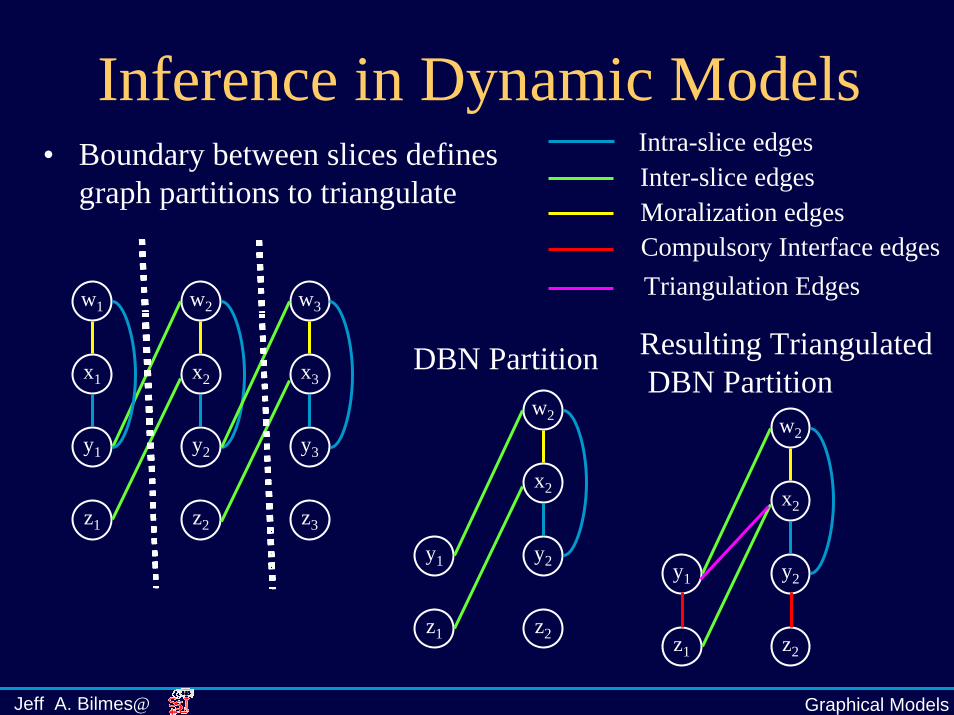
Inference in Dynamic ModelsIntra-slice edges• Boundary between slices defines

graph partitions to triangulate Inter-slice edgesMoralization edgesCompulsory Interface edges

x1

y1

w1

z1

x2

y2

w2

z2

x3

y3

w3

z3

Triangulation Edges

Resulting TriangulatedDBN Partition

DBN Partition

y1

z1

x2

y2

w2

z2

y1

z1

x2

y2

w2

z2


Inference in Dynamic Models• Each partition is stitched together to create

what is guaranteed to be a triangulated DBN

Resulting Triangulated DBN

x1

y1

w1

z1

x2

y2

w2

z2

x3

y3

w3

z3

x4

y4

w4

z4

x5

y5

w5

z5

Intra-slice edgesInter-slice edgesMoralization edgesCompulsory Interface edgesTriangulation Edges


Inference in Dynamic Models• Resulting Junction Tree (note: better ones exist, see

Bilmes&Bartels UAI’03 on triangulating DBNs)

• Junction “Tree” in this case is a Markov chain

• Not dissimilar to Hidden Markov Model alpha-recursion, but here the “cliques” oscillate between two forms.

x1

y1

w1

z1

x2

y2

w2

z2

x3

y3

w3

z3

x4

y4

w4

z4

x5

y5

w5

z5

W1,X1,Y1

Y1,Z1,W2,X2

W2,X2,Y2

Y2,Z2,W3,X3

W3,X3,Y3

Y3,Z3,W4,X4

W4,X4,Y4

Y4,Z4,W5,X5

W5,X5,Y5

Y5,Z5


Inference is Hard• NP complete (exponentially difficult) to perform

inference.• Goal: find small cliques, since complexity is

exponential in clique size (also hard, NP)• Approximate inference schemes exist for harder

problems– variational approaches– sampling techniques (MCMC, Gibbs, etc.) – loopy belief propagation (LDPC & turbo codes)– Pruning procedures


“Learning” Graphical Models• Five scenarios for learning:

1. Structure known, no hidden variables2. Structure known, hidden variables3. Structure unknown, no hidden variables4. Structure unknown, edges unknown over known

hidden variables5. Structure unknown,unknown set of hidden variables.

• Typically, we need to do 5 for speech/language/machine translation recognition.


Why Graphical Models for Speech and Language Processing

• Expressive concise way to describe properties of families of distributions

• Rapid movement from novel idea to implementation (with right toolkit) – All graphs utilize exactly same inference algorithm! Researcher concentrates on model and can stay focused on domain.

• GMs include many standard techniques but GM space is hardly explored.

• Dynamic graphical models can represent important structure in “natural” time signals but ignore what is unimportant for a given task (example parsimony through structural discriminability)


Four Main Goals for GMs in Speech/Language

1. Explicit Control: Derive graph structures that themselves explicitly represent control constructs

• E.g., parameter tying/sharing, state sequencing, smoothing, mixing, backing off, etc.

2. Latent Modeling: Use graphs to represent latent information in speech/language

3. Observation Modeling: represent structure over observations.

4. Structure learning: Derive structureautomatically, ideally to improve error rate while simultaneously minimizing computational cost.


Graph Control Structure Approaches• The “implicit” graph structure approach

– Implementation of dependencies determine sequencing through time-series model

– Everything is flattened, all edge implementations are random but are very sparse (most but not all entries are zero)

• The “explicit” graph structure approach– Graph structure itself represents control sequence mechanism

and parameter tying in a statistical model.


• Structure for the word “yamaha”, note that /aa/ occurs in multiple places preceding different phones.

Basic Triangle Structures:A basic explicit approach for parameter tying

6

aa

1

hh

5

1

Nodes & Edge Colors:

Red ⇔RANDOM

Green ⇔Deterministic


Red ⇔RANDOM


ξ

aa

4

1

y

1

1

aa

2

0

aa

2

1

m

3

1

Counter

Transition

Phone

Observation

End of word observationZweig & Russel, ‘99


Key Points• Graph explicitly represents parameter sharing• Same phone at different parts of the word are the same:

phone /aa/ in positions 2, 4, and 6 of the word “yamaha”• Phone-dependent transition indicator variables yield

geometric phone duration distributions for each phone• Counter variable ensures /aa/’s at different positions

move only to correct next phone • Some edge implementations are deterministic (green)

and others are random (red)• End of word observation, gives zero probability to

variable assignments corresponding to incomplete words.

GMs in Audio, Speech, and LanguageJeff A. Bilmes

Explicit Bi-gram Training Graph Structure

Observation

State

State Transition

State Counter

Word

End-of-Utterance Observation=1

Skip Silence

WordCounter

Word TransitionNodes & Edge Colors:

Red ⇔RANDOM



Red ⇔RANDOM


...

...


Explicit Bi-gram Training Graph Structure

Observation

State

State Transition

State Counter

Word


Skip Silence

WordCounter


Red ⇔RANDOM



Red ⇔RANDOM


...

...


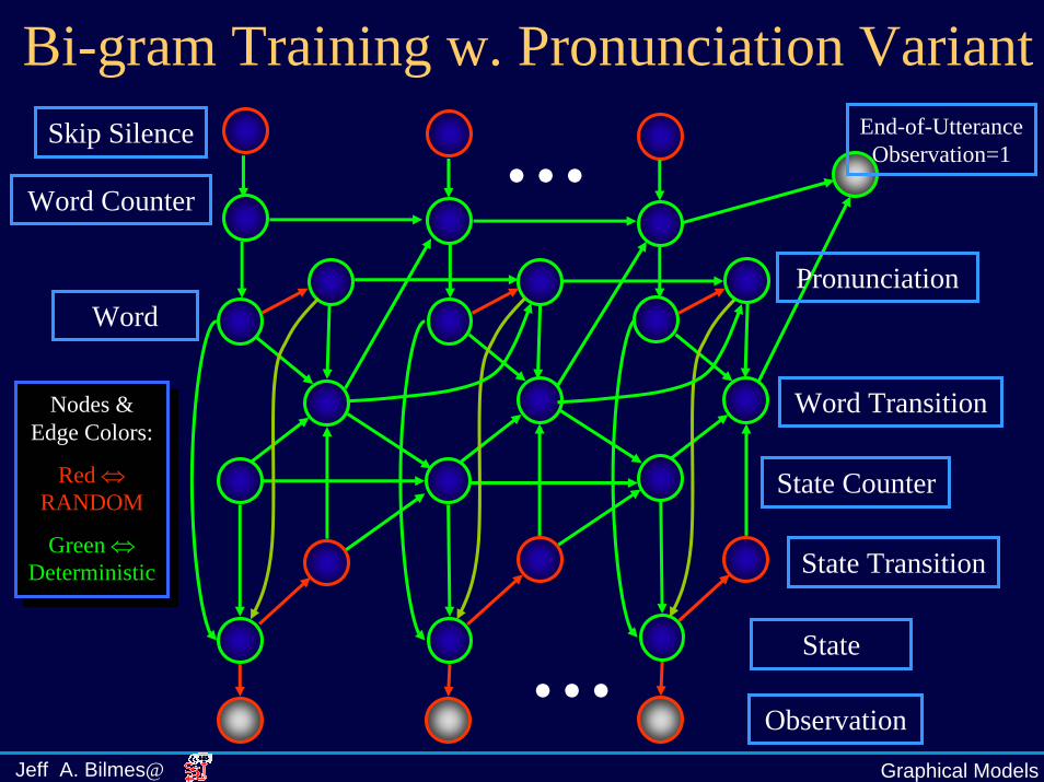
Bi-gram Training w. Pronunciation Variant

Observation

State

State Transition

State Counter

Word


Skip Silence

Word Counter


Red ⇔RANDOM



Red ⇔RANDOM


...

...Pronunciation


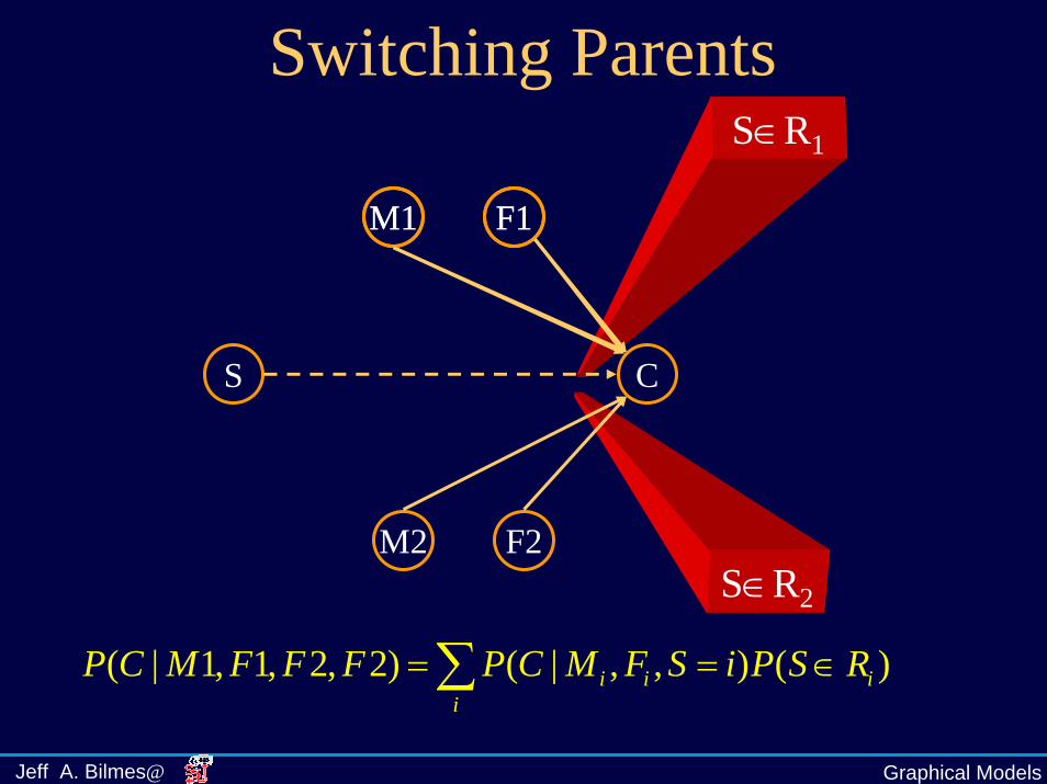
Switching Parents: Value-specific conditional independence

S∈R1

C

M1 F1

M2 F2

S

M1 F1

S∈R2

( | 1, 1, 2, 2) ( | , , ) ( )i i i ii

P C M F F F P C M F S R P S R= ∈ ∈∑


Explicit bi-gram Decoder

Nodes & Edges:

• Red ⇔RANDOM

• Green ⇔Deterministic

•Dashed line

⇔

Switching Parent

Nodes & Edges:

• Red ⇔RANDOM


•Dashed line

⇔

Switching Parent

Word

Word Transition

State Counter

State Transition

State

Observation...


WordTransition is a switching parent of Word. It switches the implementation of Word(t) to either be a copy of Word(t-1) or to invoke the bi-gram 1( | )t tP w w −


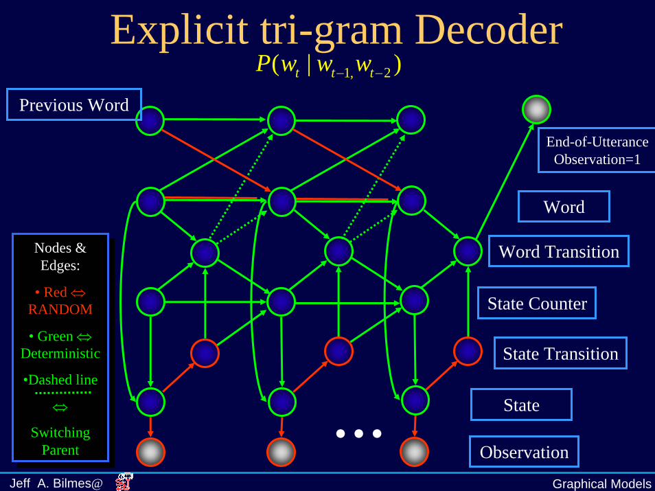
Explicit tri-gram Decoder

Word

Word Transition

State Counter

State Transition

State

Observation...


Previous Word

Nodes & Edges:

• Red ⇔RANDOM


•Dashed line

⇔

Switching Parent

Nodes & Edges:

• Red ⇔RANDOM


•Dashed line

⇔

Switching Parent

1, 2( | )t t tP w w w− −


“Auto-regressive” HMMs• Observation is no longer independent of

other observations given current state• Can not be represented by an HMM• One of the first HMM extensions tried in

speech recognition.

Q1 Q2 Q3 Q4

X1 X2 X3 X4


Observed Modeling

X

Qt-2=qt-2 Qt-1=qt-1 Qt=qt Qt+1=qt+1

Say, for this element (suppose we name it Xti)

These are the featureelements that comprise

z

The implementation of

these edges determines f(z).

Could be linear Bzor non-linear

The Hidden Variable Cloud


Buried Markov Models (BMMs)• Markov chain is “further hidden” (buried) by

specific element-wise cross-observation edges• Switching dependencies between observation

elements conditioned on the hidden chain.Q1:T=q1:T Q1:T=q’1:T


Q1:T=q1:T Q1:T=q’1:T

Multi-stream buried Markov models


Conversational M

odel

Word

Word Transition

...

Previous Word

I IIIII

AcousticModel

Observation

AcousticModel

AcousticModel

...AcousticModel

AcousticModel

AcousticModel

Cha

nnel

1C

hann

el 2

Observation

Word Transition

Word

Previous Word

End-of-Conv.


Markov Decision Processes (a digression)State of

the World

Action taken by agent

World

Policy of agent

Reward

Goal: maximize the sum of rewards, obtainable using normal forward algorithm (dynamic programming)


From Explicit Control to Latent Modeling

1. In latent modeling, we move more towards representing and learning additional information in (factored) hidden space.

2. Factored representations place constraints on what would be flattened HMM transition matrix parameters thereby potentially improving estimation quality.


Latent Modeling

Observations

Qt-2=qt-2 Qt-1=qt-1 Qt=qt Qt+1=qt+1The Hidden Variable Cloud

1:TX• Key Questions: What are the most important

“causes” or latent explanations of the temporal evolution of the statistics of the vector observation sequence?

• How best can we factor these causes to improve parameter estimation, reduce computation, etc.?


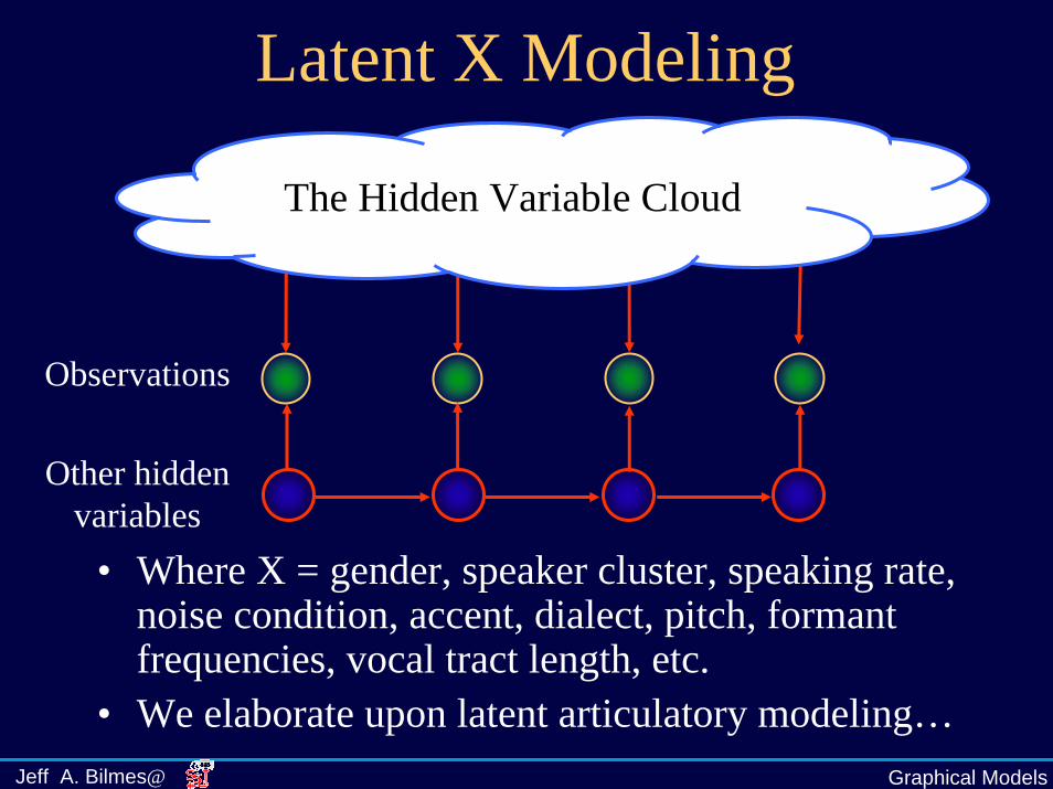
Latent X ModelingQt-2=qt-2 Qt-1=qt-1 Qt=qt Qt+1=qt+1

The Hidden Variable Cloud

Observations

Other hidden variables

• Where X = gender, speaker cluster, speaking rate, noise condition, accent, dialect, pitch, formant frequencies, vocal tract length, etc.

• We elaborate upon latent articulatory modeling…


Ex: Latent Articulatory Modeling

Pictures from Linguistics 001, University of Pennsylvania


Phone-free Articulatory Graph(by Karen Livescu)


Part of speech Tagging• Represent and find part-of-speech tags (noun,

adjective, verb, etc.) for a string of words• HMMs for word tagging

Tags

Words

• Discriminative models for this task

• Label bias issue and selection bias.

Tags

Words


Standard Language Modeling

321( | ) ( | , , )tt t ttt wP w h P w w w− −−=• Example: standard 4-gram

tW1tW −2tW −3tW −4tW −


Interpolated Uni-,Bi-,Tri-Grams

1

1 2

( | ) ( 1) ( ) ( 2) ( | )( 3) ( | , )

t t t t t t t

t t t t

P w h P P w P P w wP p w w w

α αα

−

− −

= = + =+ =

• Nothing gets zero probability


Conditional mixture tri-gram1 2

1 2 1

1 2 1 2

( | ) ( 1| , ) ( )( 2 | , ) ( | )( 3 | , ) ( | , )

t t t t t t

t t t t t

t t t t t t

P w h P w w P wP w w P w wP w w p w w w

ααα

− −

− − −

− − − −

= =+ =

+ =


Skip Bi-gram• Often there is silence between words

– “fool me once <sil> shame on <sil> shame on you”• Silence might not be good predictor of next word• But silence lexemes should be represented since

other graph modules might depend on them (e.g., acoustics, prosody, meaning in silence for MT).

• Goal: allow silence between words, but retain true word predictability skipping silence regions.

• Switching parents can facilitate such a model.


Skip Bi-gram1

1( | , ) t t

t t

r r tt t t

r w t

if w silp r w r

if w sil

δ

δ−=

−=

=⎧⎪= ⎨ ≠⎪⎩

11

1( | , )

( | ) 0tw sil t

t t tbigram t t t

if sp w s r

p w r if s

δ =

−−

=⎧⎪= ⎨ =⎪⎩( 1) Pr( )tp s silence= =


Skip bi-gram with conditional mixtures

1 1

1 1

( | ) ( 1| ) ( )

( 2 | ) ( | )bigram t t t t t

t t t t

p w r P w P w

P w P w r

α

α− −

− −

= =

+ =


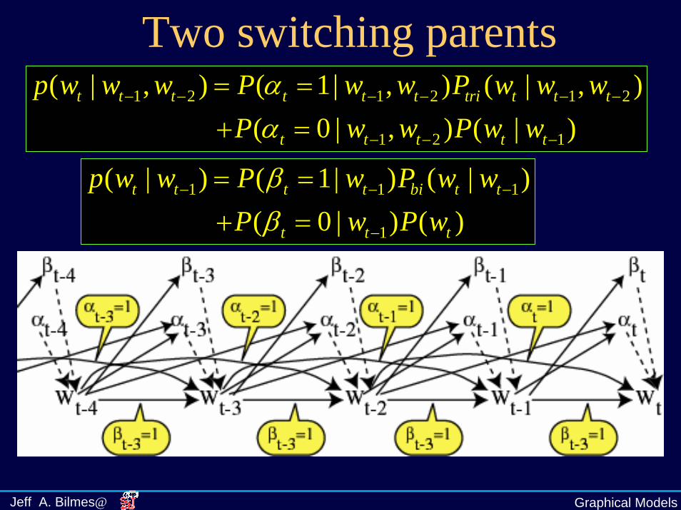
Two switching parents1 2 1 2 1 2

1 2 1

( | , ) ( 1| , ) ( | , )( 0 | , ) ( | )

t t t t t t tri t t t

t t t t t

p w w w P w w P w w wP w w P w wαα

− − − − − −

− − −

= =+ =

1 1 1

1

( | ) ( 1| ) ( | )( 0 | ) ( )

t t t t bi t t

t t t

p w w P w P w wP w P w

ββ

− − −

−

= =+ =


Skip trigram• Similar to skip bi-gram, but skips over two

previous <sil> tokens.• P(City|<sil>,York,<sil>,New) =

P(City|York,New)


Putting it together: mixture and skip tri-gram.


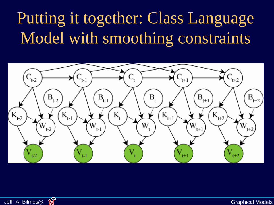
Class Language Model• When number of words large (>60k), can be

better to represent clusters/classes of words• Clusters can be grammatical or data-driven• Just an HMM (perhaps higher-order)


Explicit Smoothing• Disjoint partition of vocabulary based on training-data

counts: = {unk}∪ ∪

• = singletons, = “many-tons”, unk=unknown• ML distribution gives zero probability to unk.• Goal: Directed GM that represents and learns α:

• Word variable is like a switching parent of itself (but of course can’t be, no directed cycles allowed.)

(1 ) ( ) if( ) ( ) if

( ) otherwise

ml

ml

ml

p w unkp w p w w

p w

αα− =⎧

⎪= ∈⎨⎪⎩

S)S


Explicit Smoothing• Introduce two hidden variables K and B and one child

observed variables V=1.• Hidden variables are switching parents

– K = indicator of singleton+unk (K=1) vs. “many-ton” (K=0)– B = indicator of singleton (B=1) vs. unknown word (B=0)

• Fixed observation child V induces “reverse causal” phenomena via its dependency implementation– I.e., child says “if you want me to give you non-zero

probability on this observation, you parents had better do X”

W

V

KB


Explicit Smoothing

W

V

KB ( 1) 1 ( 0)P B P B α= = − = =

( 1) 1 ( 0) ( )P K P K P= = − = = S

( ) if 0( | , ) ( ) if 1 and 1

if 1 and 0t

M

S

w unk

p w kp w k b p w k b

k bδ =

⎧ =⎪

= = =⎨⎪ = =⎩

Singleton+unkvs. Manyton

Singleton vs. Unk

(1 ) ( ) if( ) ( ) if

( ) otherwise

ml

ml

ml

p w unkp w p w w

p w

αα− =⎧

⎪= ∈⎨⎪⎩

S)S

Goal

( 1| , ) ( , 0) or ( , 1)

or ( , 1)

{1}

P V w k w k w k

w unk k

= = ∈ = ∈ =

= =

M S

( ) if( )( )

0 else

ml

mlM

p w wpp w

⎧ ∈⎪= ⎨⎪⎩

MM

( ) if( )( )

0 else

ml

mlS

p w wpp w

⎧ ∈⎪= ⎨⎪⎩

SS


Putting it together: Class Language Model with smoothing constraints


Factored Language Models(Katrin Kirchhoff)

2tF2

1tF −22tF −

23tF −

1tF1

1tF −1

2tF −1

3tF −

3tF3

1tF −32tF −

33tF −


Switching ParentsS∈R1

C

M1 F1

M2 F2

S

M1 F1

S∈R2

( | 1, 1, 2, 2) ( | , , ) ( )i i ii

P C M F F F P C M F S i P S R= = ∈∑


“Switching Existence” Variables

• Random variables whose values determine the number of other variables in the graph

• Can represent a random number of random variables

• E.g.: can represent the length of hidden sequences, fertility in IBM models 3-5, etc.


Switching Existence: Parameter Tying and Connection to HMMs

• Parameter tying is key for implementing switching existence variables: when a new variable comes into existence, it needs some way to obtain its parameters

• Time homogeneous HMMs are also implicitly based on parameter tying, i.e., all state variables share the same transition matrix

• Probabilistic Relational Models also use a similar mechanism: a variable number of instances of an object class share the same parameters


MT Noisy Channel Graphical Model

• Goal: translate a French string,

to an English string

• Model: Noisy channel --is a noisy version of

• Inference: recover most likely given

fr

e1 e2 eM

f0 f1 fL

er

er fr

MM fffff ...211 ==

r

Lee 1=r

Observed variable

Hidden variable

Graphs by Karim Filali


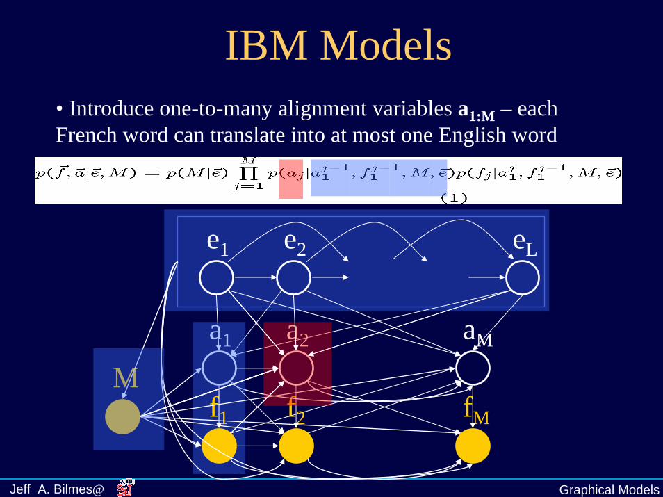
IBM Models

e1 e2 eL

f1 f2 fM

a1 a2 aM

M

• Introduce one-to-many alignment variables a1:M – each French word can translate into at most one English word


IBM Model 1

• Independence assumptions:

e2 eL

f2

a2

e1

Note: parameters for a1:M are tied(i.e. position independent)

1

f1 fM

a1 aM

L

switching parents

Existence variable


GMTK: Graphical Models Toolkit

• A GM-based software system for speech, language, and time-series modeling

• One system – Many different underlying statistical models (more than an HMM)

• Complements rather than replaces other ASR and GM systems (e.g., HTK, AT&T, ISIP, BNT, BUGS, Hugin, etc.)

• Freely available, to be open-source


GMTK Features1. Textual Graph Language2. Switching Parent Functionality3. Forwards and Backwards time links4. Multi-rate models with extended DBN templates.5. Linear Dependencies on observations6. Arbitrary low-level parameter sharing (EM/GEM training)7. Gaussian Vanishing/Splitting algorithm.8. Decision-Tree-Based implementations of dependencies

(deterministic, sparse, formula leaf nodes)9. Full inference, single pass decoding possible 10. Sampling Methods11. Linear and Island Algorithm (O(logT)) Exact Inference


GMTK Structure file for HMM• Structure file defines a prologue , chunk

, and epilog . E.g., for the basic HMM:

Q1 Q2 Q3

X1 X2 X3

Prologue, firstGroup of frames

Chunk, RepeatedUntil T frames

Epilogue, lastGroup of frames


GMTK Unrolled structure• Chunk is unrolled T-size(prologue)-

size(epilog) times (if 1 frame in chunk)

Q1

X1

Q2

X2

Q3

X3

QT

XT

QT-1

XT-1

…Prologue, first

group of framesChunk, Repeated

until T frames is obtained.Epilog, last

group of frames


Multiframe Repeating ChunksPrologue Repeating Chunk Epilogue

Prologue Chunk Unrolled 1 time Epilogue

…


GMTK Structure file for HMMframe : 0 {

variable : state {type : discrete hidden cardinality 4000;switchingparents : nil;conditionalparents : nil using DenseCPT(“pi”);

}variable : observation {

type : continuous observed 0:39;switchingparents : nil;conditionalparents : state(0) using mixGaussian mapping(“state2obs”);

}}frame : 1 {

variable : state {type : discrete hidden cardinality 4000;switchingparents : nil;conditionalparents : state(-1) using DenseCPT(“transitions”);

}variable : observation {

type : continuous observed 0:39;switchingparents : nil;conditionalparents : state(0) using mixGaussian mapping(“state2obs”);

}}


variable : S {type : discrete hidden cardinality 100;switchingparents : nil;conditionalparents : nil using DenseCPT(“pi”);

}variable : M1 {...}variable : F1 {...}variable : M2 {...}variable : F2 {...}variable : C {

type : discrete hidden cardinality 30;switchingparents : S(0) using mapping(“S-mapping”);conditionalparents :

M1(0),F1(0) using DenseCPT(“M1F1”)| M2(0),F2(0) using DenseCPT(“M2F2”);

}

GMTK Switching Structure

C

M1 F1

M2 F2

S

M1 F1


Decision-tree implementation of discrete dependencies

X1

X2

Q1

Q2 Q3

Q4 Q5 Q6 Q7

Q1(X1)=T Q1(X1)=F

PA(X2) PB(X2) PC(X2) PD(X2)


Gaussians and Directed Models

' ( ) ' ( )K U DU I B D I B= = − −

•A Gaussian can be viewed as a directed graphical model• FSICMs, obtained via U’DU factorization, provides the edge coefficients

1 1 112 13 14

2 2 223 24

3 3 334

4 4 4

00 00 0 00 0 0 0

x xb b bx xb bx xbx x

εεεε

⎡ ⎤ ⎡ ⎤ ⎡ ⎤⎡ ⎤⎢ ⎥ ⎢ ⎥ ⎢ ⎥⎢ ⎥⎢ ⎥ ⎢ ⎥ ⎢ ⎥⎢ ⎥= +⎢ ⎥ ⎢ ⎥ ⎢ ⎥⎢ ⎥⎢ ⎥ ⎢ ⎥ ⎢ ⎥⎢ ⎥⎢ ⎥ ⎢ ⎥ ⎢ ⎥⎣ ⎦⎣ ⎦ ⎣ ⎦ ⎣ ⎦

X1 X2 X3 X4( ) ( | )i

ii

f x f x xπ=∏


GMTK Splitting/Vanishing Algorithm

• Determines number Gaussian components/state• Split Gaussian if it’s component probability

(“responsibility”) rises above a number-of-components dependent threshold

• Vanish Gaussian if it’s component probability falls below a number-of-components dependent threshold

• Use a splitting/vanishing schedule, one set of thresholds per each EM training iteration.


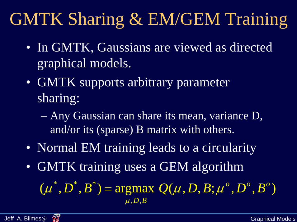
GMTK Sharing & EM/GEM Training• In GMTK, Gaussians are viewed as directed

graphical models.• GMTK supports arbitrary parameter

sharing: – Any Gaussian can share its mean, variance D,

and/or its (sparse) B matrix with others.• Normal EM training leads to a circularity• GMTK training uses a GEM algorithm

* * *

, ,( , , ) argmax ( , , ; , , )o o o

D BD B Q D B D B

µµ µ µ=


Exact inference in DBNs• Triangulation in DBNs

– Standard triangulation heuristics typically poor for DBNssince they are short and wide

– Slice-by-slice triangulation via elimination: severely limit number of elimination orders without limiting optimal triangulation quality

– Triangulation quality is lower-bounded by size of interface to previous (or next) slice

– Can allow interfaces to span multiple slices, which can make interface quality much better (“On Triangulating Dynamic Graphical Models, UAI’2003,”, Bilmes & Bartels).

• Use message passing order in junction tree that respects directed deterministic dependencies when possible (to cut down on state space)


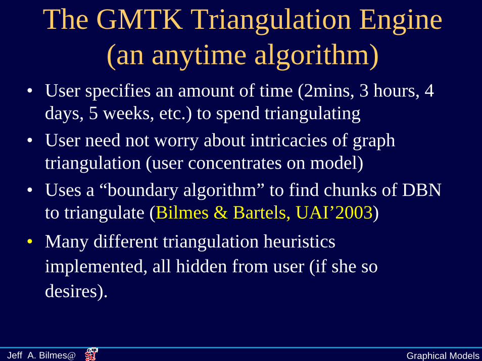
The GMTK Triangulation Engine(an anytime algorithm)

• User specifies an amount of time (2mins, 3 hours, 4 days, 5 weeks, etc.) to spend triangulating

• User need not worry about intricacies of graph triangulation (user concentrates on model)

• Uses a “boundary algorithm” to find chunks of DBN to triangulate (Bilmes & Bartels, UAI’2003)

• Many different triangulation heuristics implemented, all hidden from user (if she so desires).


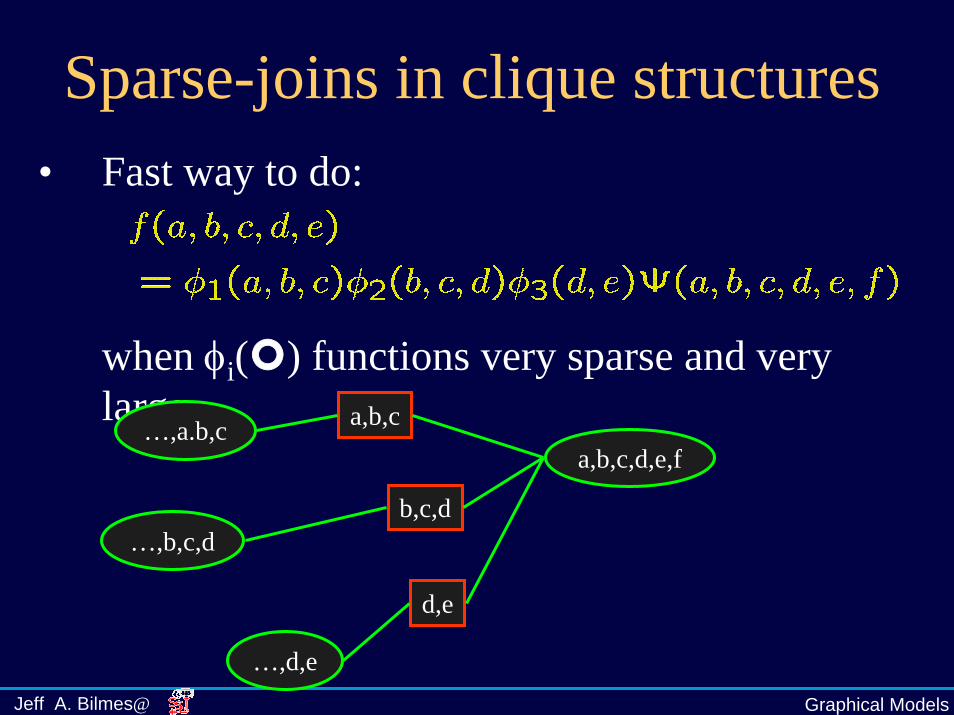
Sparse-joins in clique structures• Fast way to do:

when φi( ) functions very sparse and very large.

a,b,c,d,e,fa,b,c

b,c,d

d,e

…,a.b,c

…,b,c,d

…,d,e


Linear and Island Algorithm (log space) exact inference

• Exact inference O(T*S) space and time complexity, S = clique state space size

• Log-space inference O(log(T)*S) space at an extra cost of a factor of log(T) time.

• Can use both linear and log space inference at same time (for optimal tradeoff).

• This is called the Island Algorithm (Binder et. al. 1997)


Example: Linear-Space in HMM( ) ( 1) ( )i j ji i t

jt t a b xα α= −∑

1( ) ( 1) ( )i j ij j tj

t t a b xβ β += +∑


Example: One recursions Log Space( ) ( 1) ( )i j ji i t


1( ) ( 1) ( )i j ij j tj

t t a b xβ β += +∑


Example: Two recursions Log Space( ) ( 1) ( )i j ji i t


1( ) ( 1) ( )i j ij j tj

t t a b xβ β += +∑


GMTK is infrastructure• GMTK does not solve speech and language

processing problems, but provides tools to help to simplify testing modeling, and does so in novel ways.

• The space of possible solutions is quite large, and its exploration has only just started.


Current StatusCurrent StatusI. Old version (developed by Jeff Bilmes & Geoff

Zweig) available at:A. http://ssli.ee.washington.edu/~bilmes/gmtkB. ~100 pages of documentationC. Book chapter on use of graphical models for speech

and languageD. JHU’2001 Workshop technical report

II. New Version Running, Much Faster and with many new features. End Summer’04 beta release.

http://ssli.ee.washington.edu/~bilmes/gmtk


Other GM Toolkits• Best place to look:

http://www.ai.mit.edu/~murphyk/Software/BNT/bnsoft.html contains a great comparison of various toolboxes.

• GMTK – optimized for speech/language and DBNs. Summer’04 version will be even more so.

• Other tools– HTK– AT&T Finite State Tools

http://www.ai.mit.edu/~murphyk/Software/BNT/bnsoft.html




DiscussionDiscussion• Questions?• Ideas?• Confusion?• Suggestions?• Please ask.


Conclusions• Graphical Models are very flexible!!• With right toolkit, possible to rapidly build up a

novel statistical idea.• Space of models is still relatively unexplored,

young research area for speech/language/NLP.


The Endthank you!


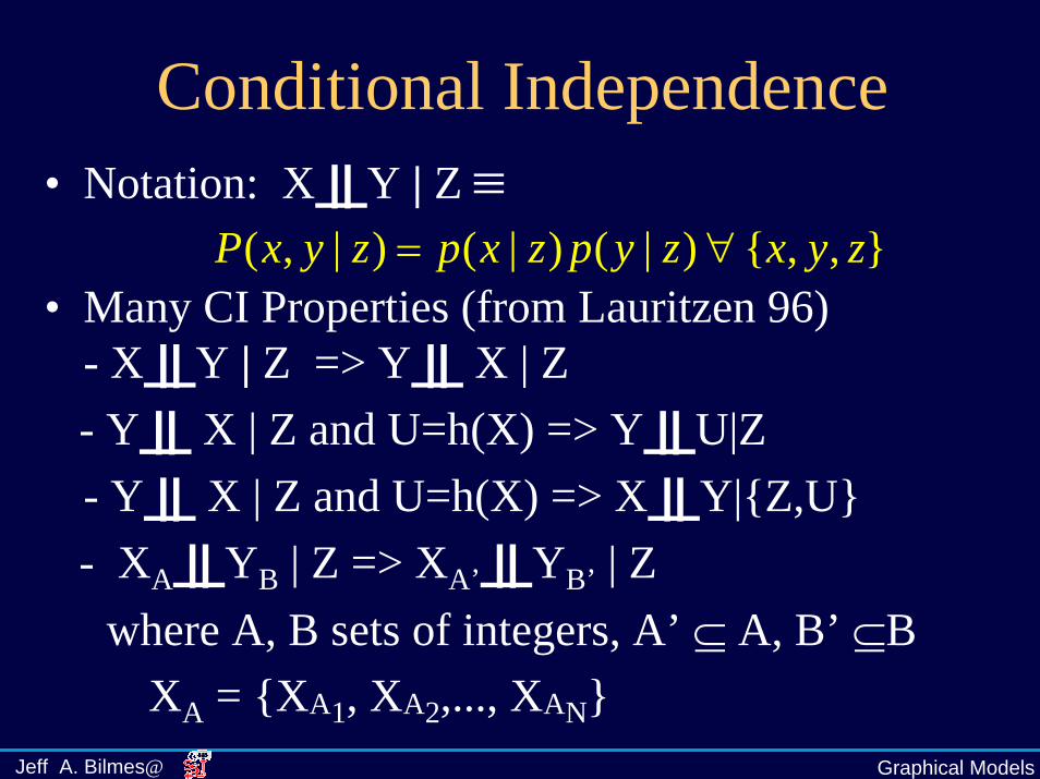
Conditional Independence• Notation: X || Y | Z ≡

• Many CI Properties (from Lauritzen 96)- X || Y | Z => Y || X | Z- Y || X | Z and U=h(X) => Y || U|Z- Y || X | Z and U=h(X) => X || Y|{Z,U}- XA || YB | Z => XA’ || YB’ | Z

where A, B sets of integers, A’ ⊆ A, B’ ⊆BXA = {XA1, XA2,..., XAN}

},,{)|()|()|,( zyxzypzxpzyxP ∀=

graphical models in speech and language...

Documents