Graphical diagnostics of endogeneity∗

Xavier de Lunaa and Per Johanssonba Department of Economics, Umea University,

S-90187 Umea, Sweden.

E-mail: xavier.deluna@econ.umu.seb IFAU - Office of Labour Market Policy Evaluation,

S-75120 Uppsala, Sweden.

E-mail: per.johansson@ifau.uu.se

Abstract

We show that in sorting cross-sectional data, the endogeneity ofa variable may be successfully detected by graphically examining thecumulative sum of the recursive residuals. An interesting case ariseswith a continuous or ordered (e.g., years of schooling) endogenous vari-able. Then, a graphical test for misspecification due to endogeneity(e.g., self selection) can be obtained without instrumental variables.Moreover, the sign of the bias implied by this endogeneity becomesdeducible through such graphs.

Keywords: CUSUM plot; Recursive residuals; Return to schooling;Self selection.

JEL: C32, C52.

∗The first author would like to acknowledge the Wikstrom Foundation for its financialsupport.

1

1 Introduction

In regression models for continuous responses, all sorts of model misspecifi-cations may be diagnosed by an analysis of ordinary residuals, i.e., from anordinary least square (OLS) estimator. Endogeneity of variables is a notableexception, however; with linear models, this is due to the OLS estimatedparameter being consistent for the reduced form parameter (other than thestructural parameter).The purpose of this paper is to show how recursive residuals associated

with a specific ordering of the data can be successfully analyzed in orderto diagnose the endogeneity of a variable. In particular, we show that agraphical display of the cumulative sum of the recursive residuals obtainedby assuming exogeneity is helpful in diagnosing the presence of endogeneity.Moreover, the sign of the bias implied by this endogeneity (e.g., the directionof a self selection bias) is also deducible through such graphs. The useof recursive residuals was earlier advocated by Harvey and Collier (1977) totest for functional misspecification in regression analysis.1 In particular, theyproposed a t-statistic to test that the residuals have expectation zero. Thistest is directly applicable to test against endogeneity when the data is sortedadequately. Instruments may be needed to obtain such a sorting.However, an interesting case arises with a continuous or ordered (e.g.,

years of schooling) variable whose endogeneity is due to selectivity. Sortingthe data with respect to this variable and looking at recursive residuals ob-tained with a model where exogeneity is assumed allow us to diagnose themisspecification. In this case, endogeneity can thus be diagnosed withoutspecifying a model for the alternative, in contrast with the Hausman test (cf.Hausman, 1978) for which certain instruments are needed.In Section 2, we start by presenting a framework allowing us to intro-

duce special orderings of the data that are useful for diagnosing endogeneity.Section 3 presents the methodology based on the calculation of recursiveresiduals associated with a relevant ordering of the data. Graphical displaysof these residuals as well as the Harvey-Collier test statistic are proposedto diagnose the endogeneity of a variable. Sections 4 to 6 present differentareas of application. Thus, Section 4 looks at a text-book example of en-dogeneity due to simultaneity of two variables. Section 5 considers Garen’s

1Endogeneity of a variable is often equivalent to a functional misspecification. Forinstance, if a random coefficient is associated to a continuous endogenous variable (e.g.Garen’s (1984) model), the outcome equation is implicitely non-linear in that variable.

2

(1984) model of selectivity based on a random coefficient. In particular, areal data set concerning returns to schooling is analyzed in detail. Finally,Section 6 discusses the case of endogenous treatment where the propensityscore (Rosenbaum and Rubin, 1983) can be used to sort the data to identifyself-selection. The paper is concluded with a discussion in Section 7.

2 Sorting scores for endogeneity

We consider an observational study where independent observations are avail-able for a response y, together with a set of exogenous variables x and apossibly endogenous variable z (denoted the treatment in the sequel). Thefollowing linear statistical model is considered

y = x0β + γz + ε,

where ε is a zero mean error term. The exogeneity of x implies that itsmarginal density, p(x; δ), δ ∈ D ⊆ Rd, can be ignored without loss of infor-mation about β and γ (see, e.g., Gourieroux and Monfort, 1995, Chap. 1.5).Similarly, if treatment z is exogenous, its effect can be studied by the solespecification of p(y|z,x;β, γ), that is, the density of the error term. How-ever, in a typical observational study, the exogeneity of treatment z must beassessed.We propose graphical diagnostics of endogeneity by sorting the data with

respect to a sorting score. The sorted data should then not be distinguishablefrom any other random ordering, only under the exogeneity of the variableof interest.In general, there is no unique sorting score for a given problem, but certain

sorting scores will be more useful than others. In order to present results, wemust give a minimal description of the alternative hypothesis of endogeneity.Hence, let us consider an unobserved variable u such that

E(ε|x, z, u) = u. (1)

Let

m(x, z;θ) = x0β + γz,

where θ = (β0, γ)0. Under H0 : ”z is exogenous”, implying within this frame-work that E(u|x, z) = 0, we have that m(x, z;θ) = E(y|z,x), the unbiased

3

and optimal (with minimum mean squared error of prediction) predictor ofy, given x and z.Let us define θc (possibly a function of c) as

θc = argminθE[y −m(x,z;θ)2|z,x, s < c],

where s is a random variable. We call this variable a sorting score when it issuch that θc = θ, a constant, only under H0. Such sorting scores will allowus to identify endogeneity by fitting m(x, z;θc) recursively to data sortedwith respect to s and looking for evidence of a varying parameter θc. Wenow define a class of particularly useful sorting scores.

Definition 1 A monotone sorting score s for E(y|x, z) is such that ∀c ∈ Ωs,

m(x, z;θc) ≶ E(y|z,x) for all x, z such that s > c,when H0 does not hold.

We start by a preliminary result.

Lemma 1 If u = λz, and hence sorting with respect to u or z is identical,then for s = u, ∀c ∈ Ωs, m(x, z;θc) = E(y|z,x) for all x, z.Proof. We have that E(y|z,x) = x0β + (γ + λ)z. Moreover, θc is solutionof

E(y −m(x, z;θc)|z,x, s < c) = 0,∀c ∈ Ωs. But here, E(y −m(x, z;θc)|z,x, s < c) = E(y −m(x, z;θc)|z,x)and θc = (β

0, γ + λ)0. The lemma is then proved.Thus, in the situation of the lemma, s = u is not monotone and will not

help us identify endogeneity. In fact, λ and γ are not identifiable in such asituation. On the other hand, let u and z be not proportional but linearlydependent as

u = ξ1z + ξ2, (2)

where ξi, i = 1, 2 are random variables with E(ξi|x, z) = αi, α1 6= 0, andV (ξi|x, z) ≥ 0, for any z. The latter inequality is assumed to be strict forat least one i, i = 1, 2. Furthermore, when V (ξ1|x, z) > 0, z is assumed tobe either always non-negative or always non-positive. Then, it can be shownthat u is a monotone sorting score:

4

Proposition 1 Let u in (1) be such that under endogeneity of z, u and zare linearly dependent as described by (2). Then, u is a monotone sortingscore.

Proof.We assume endogeneity of z. We can write

E(y|x, z, u) = β0x+ γz + u

and

E(y|x, z) = β0x+ γz +E(u|x,z),where E(u|x, z) 6= 0. Furthermore, for a constant c ∈ Ωu (the sample spaceof u),

E(y|x, z, u < c) = β0x+ γz +E(u|x, z, u < c).By the linearity assumption (2), we can write E(u|x, z, u < c) = αc2 + αc1z,where αci = E(ξi|x, z, u < c), i = 1, 2, are constants although functions of c.Hence,

E(y|x, z, u < c) = β0x+ γz + αc2 + αc1z,

which is linear and equivalent to m(x, z; θc). Moreover, because αci < αiwhen V (ξi|x, z) > 0 (this is true for at least one i), E(u|x, z, u < c) <E(u|x, z) for any positive z and E(u|x, z, u < c) > E(u|x, z) for any negativez. Thereby the monotonicity of u as sorting score is implied.Even if u is unobserved, this result is of practical use because the ordering

of u can be retrieved by studying z and its relation to certain instruments,see the example sections below.A most convenient case arises when z is a monotone sorting score in itself,

since no instrumental variables are then required. This situation can arisewhen E(u|z) is non-linear in z which is, for instance, the case with randomcoefficient models; see Section 5.

3 Graphical diagnostics

Graphical diagnostics are informal tools for analysis but, at the same time,a very powerful medium for conveying information. A graph may tell morethan the value of a test statistic, although both are obviously complementary.Since ordinary residuals are not really appropriate to identify the endogeneitymisspecification, we base our analysis on recursive residuals.

5

3.1 Recursive residuals

Let a set of independent observations (yi,xi, zi), i = 1, . . . , n, be generatedby a model with corresponding density p(y|z,x;β). For each k = q, . . . , n−1,a consistent estimate bβk of β, based on (yi,xi, zi), i = 1, . . . , k, is assumedto be available. Recursive residuals are then obtained by predicting yj with

E(yj|zj,xj; bβj−1), j = q + 1, . . . n. This prediction is an estimate, based onobservations (yi,xi, zi), i = 1, . . . , j − 1, of the optimal (mean squared errorsense) predictor E(yj|zj,xj;β). The recursive residuals are then standardizedprediction errors:

wj =yj − E(yj|zj,xj; bβj−1)

V ar(yj −E(yj|zj,xj; bβj−1)|zj,xj) , j = q + 1, . . . n.

Assuming that the involved moments exist and that the model is well spec-ified, these recursive residuals are, at least asymptotically, independent andidentically distributed with mean zero and variance one. These propertieshold exactly when β is known.

Example 1 The linear Gaussian model, yi = x0iβ+ εi with εi independently

and normally distributed with mean zero and variance σ2, is an importantparticular case for which recursive residuals were originally studied, e.g., byBrown et al. (1975). For this model, we have, for j = q + 1, . . . n,

wj =yj − x0jbβj−1

σ(1 + x0j(X0j−1Xj−1)−1xj)1/2

,

where Xj−1 = (x01, . . . ,x0j−1)

0. Assuming that X0j−1Xj−1 are invertible, wj

are homoscedastic, independent, and with standard normal distribution (Brownet al., 1975). No asymptotic argument is needed here.

Kianifard and Swallow (1996) review the application of recursive residu-als, see also Dawid (1984) and de Luna and Johansson (2000).

3.2 Cumulative sum and the Harvey-Collier test

A graphical diagnostic tool is obtained by graphically displaying recursiveresiduals. Their cumulative sum (CUSUM) is most useful. Asymptotically,

6

the recursive residuals have mean zero for a well-specified model. When miss-specification arises, in our case when exogeneity of the treatment does nothold, the recursive residuals will typically have non-zero mean. If we thensort the data with respect to s, a monotone sorting score, the residuals willhave positive (or negative) mean throughout the recursion.The results of Section 2 can be used to obtain such sortings. In the

time series context, the aim when inspecting cumulative sums is to detect achange of the parameter values, see e.g. Brown et al. (1975). Most oftenthis is believed to be an abrupt structural change at a unknown point intime. The endogeneity misspecification is instead translated by small butsystematic biases in predictions. Thus, a monotone sorting score shouldbe used for these biases to accumulate instead of cancelling each other out,thereby guaranteeing the best visual effect when plotting the cumulative sumof the recursive residuals. Examples illustrate these issues in the next section.The constancy of the bias sign is also relevant for the test presented belowto have power.Harvey and Collier (1977) proposed a simple test based on the sum of

the recursive residuals to identify functional misspecification in a regressionmodel. In our context, write

w =1

n− qnX

i=q+1

wi

the average of the recursive residuals. Then, under H0, asymptotically (ex-actly under the normal model), w is normally distributed with mean zeroand variance 1/(n − q), and constitutes a test statistic for H0. This test isa necessary complement to the CUSUM plot. Note that a simulation studyconducted in de Luna and Johansson (2000) showed the good properties ofthe Harvey-Collier test in comparison with, for example, a classic Hausmantest.

4 Application I: consumption and income

Consider the model for y and z:

y = βx1 + γz + ε,

7

where variable z is endogenous, such that

z = αx2 + ν,

with ε and ν correlated2. Denote x = (x1, x2). Assuming E(ε|ν) to be linearin ν (e.g., bivariate normality), we have

E(y|x, z) = βx1 + γz + λ(z − αx2), (3)

where λ = 0 if and only if ε and ν are uncorrelated. Here, s = (z − αx2) ischosen as a sorting score. Note that λs(x2, z) plays the role of the omittedvariable u in (1). The assumptions of Proposition 1 are met when, for in-stance, x2 and z are jointly normal

3 (so that E(x2|z) is linear in z), in whichcase we can say that s is a monotone sorting score. It can be approximatedby (z− bαx2), where bα is a consistent estimate. Note that x2 = x1 would leadto the non-identifiability of γ, and the non-applicability of Proposition 1.

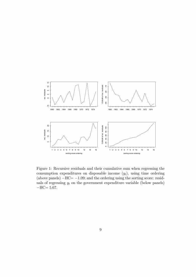
Example 2 We use data on U.S. consumption expenditures (ct), disposableincome (yt) and government expenditure (gt), in billions of 1982 dollars, foryear t between 1975-1986.4 We assume:

ct = γ0 + γ1yt + εt,

where yt is endogenous such that

yt = α0 + α1gt + νt. (4)

Figure 8 shows how the endogeneity of yt is revealed by using the residualsfrom (4) as a sorting score.

2Classical examples include: i) y is a quantity of goods and z its price, ii) y is aconsumption measure and z disposable income.

3This assumption might seem restrictive, but is only needed to ensure that Proposition1 can be applied. It should be observed, however, that the linearity of E(s|z) is not anecessary condition for monotonicity.

4This data is described in Hill, Griffiths and Judge (1997) and obtained fromhttp:\\www.wiley.com.

8

rec.

resi

dual

s

1960 1962 1964 1966 1968 1970 1972 1974

-15

-50

510

15

CU

SUM

of r

ec. r

esid

uals

1960 1962 1964 1966 1968 1970 1972 1974

-40

-30

-20

-10

sorting score ordering

rec.

resi

dual

s

1 2 3 4 5 6 7 8 9 10 12 14 16

510

1520

sorting score ordering

CU

SUM

of r

ec. r

esid

uals

1 2 3 4 5 6 7 8 9 10 12 14 16

020

4060

8010

0

Figure 1: Recursive residuals and their cumulative sum when regressing theconsumption expenditures on disposable income (yt), using time ordering(above panels) −HC= −1.09; and the ordering using the sorting score: resid-uals of regressing yt on the government expenditure variable (below panels)−HC= 5.67.

9

5 Application II: return to schooling

5.1 The Garen model

We now consider the selectivity model proposed by Garen (1984, 1988)

y = x0β + zδ + zr + ε, (5)

z = f(x∗) + ν,

where E(ε|x∗, z, r) = 0 and x∗ contains all the variables in x and possiblyothers.5 For this model,

E(y|x∗, z) = x0β + zδ + zE(r|ν). (6)

AssumingE(r|ν) to be linear in ν (e.g., bivariate normality), we haveE(r|ν) =λ(z − f(x∗)). Exogeneity of z corresponds to λ = 0, i.e. uncorrelated r andν variables. Here, heteroscedasticity is present even if z is exogenous:

V (y|x∗, z) = z2V (r|ν) + σ2, (7)

where σ2 is the variance of ε. In this case, neglecting the endogeneity of zleads to a misspecification of the conditional expectation, by assuming it tobe linear while zE(r|ν) is non-linear in x∗ and z.In this example, not accounting for the endogeneity of z corresponds to

omitting the variable6 z(z − f(x∗)) in (6) which corresponds to u in (1).The non-linearity of E(y|x, z) may often be hidden by the heteroscedasticnoise when examining conventional residuals. On the other hand, recursiveresiduals can often identify the systematic bias in predictions obtained withthe sorting score s = z(z − f(x∗))7 as illustrated in Example 3. Becausef is unknown, an approximate sorting score must be used to estimate thisfunction, yielding z(z − bf(x∗)). Notice that within this framework, it ispossible to proceed without specifying a parametric form for f but insteadusing a non-parametric estimate.

5Garen also considered a pure random effect, i.e. y = x0β + zδ + zr + η + ε, withE(y|x∗, z) = x0β + zδ + zE(r|ν) +E(η|v) and E(η|v) = ρv. Here, we omit η for clarity.

6The omitted variable is a sorting score since λ = 0 under exogeneity.7Note that Proposition 1 does not apply here since E(s|z) is not linear in z. However,

E(s|z) is quadratic in z and therefore, fitting a linear model in z leads to a systematicunder-prediction of y and hence, s is a monotone sorting score.

10

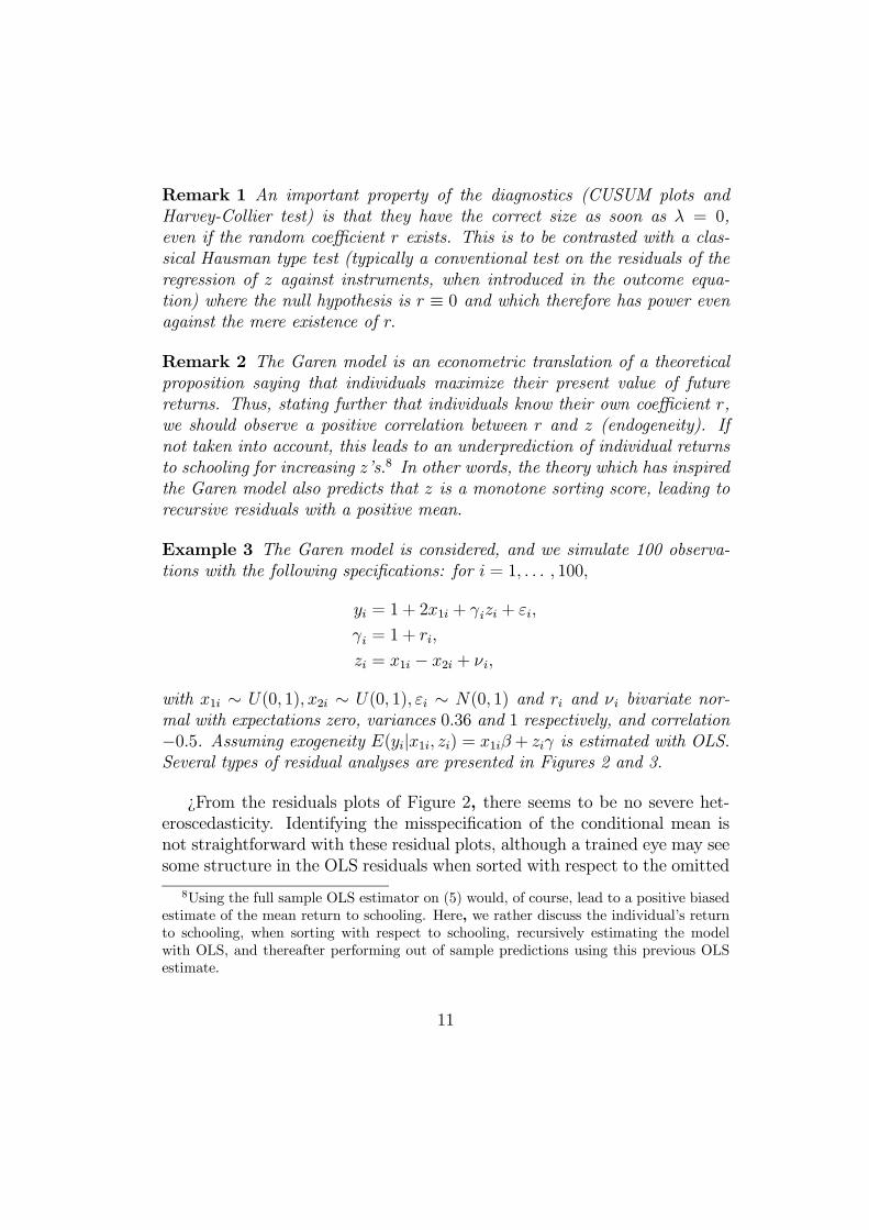
Remark 1 An important property of the diagnostics (CUSUM plots andHarvey-Collier test) is that they have the correct size as soon as λ = 0,even if the random coefficient r exists. This is to be contrasted with a clas-sical Hausman type test (typically a conventional test on the residuals of theregression of z against instruments, when introduced in the outcome equa-tion) where the null hypothesis is r ≡ 0 and which therefore has power evenagainst the mere existence of r.

Remark 2 The Garen model is an econometric translation of a theoreticalproposition saying that individuals maximize their present value of futurereturns. Thus, stating further that individuals know their own coefficient r,we should observe a positive correlation between r and z (endogeneity). Ifnot taken into account, this leads to an underprediction of individual returnsto schooling for increasing z’s.8 In other words, the theory which has inspiredthe Garen model also predicts that z is a monotone sorting score, leading torecursive residuals with a positive mean.

Example 3 The Garen model is considered, and we simulate 100 observa-tions with the following specifications: for i = 1, . . . , 100,

yi = 1 + 2x1i + γizi + εi,

γi = 1 + ri,

zi = x1i − x2i + νi,

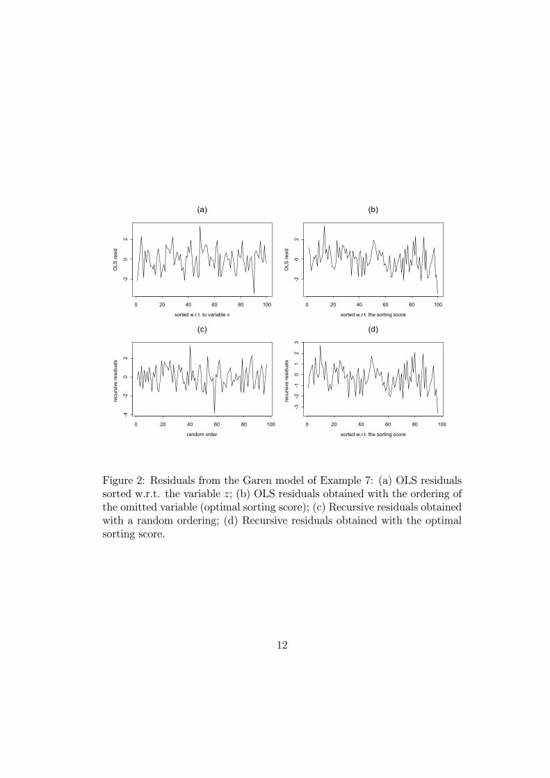
with x1i ∼ U(0, 1), x2i ∼ U(0, 1), εi ∼ N(0, 1) and ri and νi bivariate nor-mal with expectations zero, variances 0.36 and 1 respectively, and correlation−0.5. Assuming exogeneity E(yi|x1i, zi) = x1iβ + ziγ is estimated with OLS.Several types of residual analyses are presented in Figures 2 and 3.

¿From the residuals plots of Figure 2, there seems to be no severe het-eroscedasticity. Identifying the misspecification of the conditional mean isnot straightforward with these residual plots, although a trained eye may seesome structure in the OLS residuals when sorted with respect to the omitted

8Using the full sample OLS estimator on (5) would, of course, lead to a positive biasedestimate of the mean return to schooling. Here, we rather discuss the individual’s returnto schooling, when sorting with respect to schooling, recursively estimating the modelwith OLS, and thereafter performing out of sample predictions using this previous OLSestimate.

11

sorted w.r.t. to variable x

OLS

resi

d

0 20 40 60 80 100

-20

2

(a)

sorted w.r.t. the sorting score

OLS

resi

d

0 20 40 60 80 100

-20

2

(b)

random order

recu

rsiv

e re

sidu

als

0 20 40 60 80 100

-4-2

02

(c)

sorted w.r.t. the sorting score

recu

rsiv

e re

sidu

als

0 20 40 60 80 100

-3-2

-10

12

3

(d)

Figure 2: Residuals from the Garen model of Example 7: (a) OLS residualssorted w.r.t. the variable z; (b) OLS residuals obtained with the ordering ofthe omitted variable (optimal sorting score); (c) Recursive residuals obtainedwith a random ordering; (d) Recursive residuals obtained with the optimalsorting score.

12

sorted w.r.t. the sorting score

CU

SUM

of O

LS re

sid

0 20 40 60 80 100

05

1015

(a)

random order

CU

SUM

of r

ecur

sive

resi

dual

s

0 20 40 60 80 100

-22

46

8

(b)

sorted w.r.t. the sorting score

CU

SUM

of r

ecur

sive

resi

dual

s

0 20 40 60 80 100

-25

-15

-55

(c)

sorted w.r.t. the estimatedsorting score

CU

SUM

of r

ecur

sive

resi

dual

s

0 20 40 60 80 100

-25

-15

-5

(d)

sorted w.r.t. to variable z

CU

SUM

of r

ecur

sive

resi

dual

s

0 20 40 60 80 100

-30

-10

(e)

sorted w.r.t. residuals from regress.of z against x

CU

SUM

of r

ecur

sive

resi

dual

s

0 20 40 60 80 100

-40

-20

0

(f)

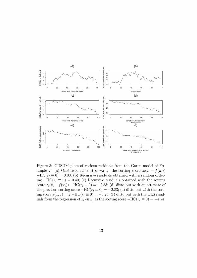
Figure 3: CUSUM plots of various residuals from the Garen model of Ex-ample 2: (a) OLS residuals sorted w.r.t. the sorting score zi(zi − f(xi))−HC(ri ≡ 0) = 0.00; (b) Recursive residuals obtained with a random order-ing −HC(ri ≡ 0) = 0.40; (c) Recursive residuals obtained with the sortingscore zi(zi − f(xi)) −HC(ri ≡ 0) = −2.53; (d) ditto but with an estimate ofthe previous sorting score −HC(ri ≡ 0) = −2.83; (e) ditto but with the sort-ing score s(x, z) = z −HC(ri ≡ 0) = −3.75; (f) ditto but with the OLS resid-uals from the regression of zi on xi as the sorting score −HC(ri ≡ 0) = −4.74.

13

variable, graph (b), and in the recursive residuals obtained with this samesorting score, graph (d). The CUSUM plots in Figure 3 are more interest-ing. We note that the recursive residuals obtained with well chosen sortingscores all provide a clear sign of the misspecification of the conditional meanof the model (endogenous treatment) by displaying a systematic departurefrom zero for the CUSUM trajectory. This neat visual effect is due to themonotonicity property. Note that, as in Section 4, the residuals of the selec-tion equation as well as the endogenous variable itself also seem to providemonotone sorting scores, see the bottom panel of Figure 3. The values ofthe HC test (for H0 : ri ≡ 0), given in the caption of the figure, confirm thevisual impression.

5.2 U.S. data on return to schooling

The data set9 analyzed in this section was used by Angrist and Krueger(1991) to study the effects of compulsory school attendance, see also Angristet al. (1999). It consists of a sample of 329 500 men born in 1930-39 from the1980 US census. This data set will help us illustrate the kind of insights agraphical display of CUSUM recursive residuals can yield when investigatingthe exogeneity of a covariate.The linear model of interest tries to explain the log weekly wage by the

number of schooling years, while controlling for an age effect (assumed to beexogenous). Schooling systems differ between states, see Angrist and Krueger(1991, Appendix 2), and for that reason, we perform state-specific analyses.As argued in the previous section, the explanatory variable describing schoolattendance can be used as sorting score to check its endogeneity which ispredicted by the theory. We discard individuals with zero to eleven years ofeducation, in order to avoid effects due to compulsory schooling laws.10 Inparticular, the compulsory schooling period should not suffer from a selectionbias.Recursive residuals are computed starting from 13 years of education, 1-

12 years cases serving as starting values, together with one individual with 13years to allow for estimability.11 In a sense, the question of interest is whether

9The data set is available at the following address: http://qed.econ.queensu.ca/jae/10Compulsory schooling laws may in some instances push students to complete a high

school degree, see Angrist and Krueger (1991, pp. 1004-1005).11In this application, we have multiple observations for a given number of years of

eduction. These are left in their original ordering.

14

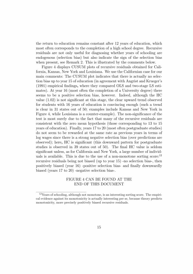
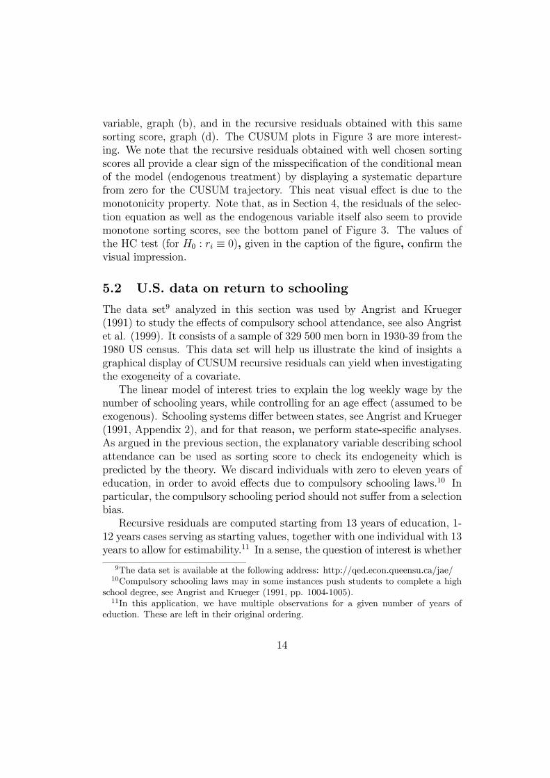
the return to education remains constant after 12 years of education, whichmost often corresponds to the completion of a high school degree. Recursiveresiduals are not only useful for diagnosing whether years of schooling areendogenous (selection bias) but also indicate the sign of the selection biaswhen present, see Remark 2. This is illustrated by the comments below.Figure 4 displays CUSUM plots of recursive residuals obtained for Cali-

fornia, Kansas, New York and Louisiana. We use the Californian case for ourmain comments: The CUSUM plot indicates that there is actually no selec-tion bias up to year 15 of education (in agreement with Angrist and Krueger’s(1991) empirical findings, where they compared OLS and two-stage LS esti-mates). At year 16 (most often the completion of a University degree) thereseems to be a positive selection bias, however. Indeed, although the HCvalue (1.02) is not significant at this stage, the clear upward trend observedfor students with 16 years of education is convincing enough (such a trendis clear in 31 states out of 50; examples include Kansas and New York inFigure 4, while Louisiana is a counter-example). The non-significance of thetest is most surely due to the fact that many of the recursive residuals areconsistent with the zero mean hypothesis (those corresponding to 13 to 15years of education). Finally, years 17 to 20 (most often postgraduate studies)do not seem to be rewarded at the same rate as previous years in terms oflog wages since there is a strong negative selection bias (over predictions areobserved); here, HC is significant (this downward pattern for postgraduatestudies is observed in 39 states out of 50). The final HC value is seldomsignificant unless, as for California and New York, a large number of individ-uals is available. This is due to the use of a non-monotone sorting score:12

recursive residuals being not biased (up to year 15) -no selection bias-, thenpositively biased (year 16) -positive selection bias- and finally downwardlybiased (years 17 to 20) -negative selection bias-.

FIGURE 4 CAN BE FOUND AT THEEND OF THIS DOCUMENT

12Years of schooling, although not monotone, is an interesting sorting score. The empiri-cal evidence against its monotonicity is actually interesting per se, because theory predictsmonotonicity, more precisely positively biased recursive residuals.

15

Figure 4: Vertical bars indicate years of education; for instance, residualsbefore the first bar correspond to 13 years, residuals between the first andthe second bar are for individuals with 14 years of education and so on, upto 20 years. HC values are: -2.13 for California, 0.73 for Kansas, -5.23 forNew York and -1.34 for Louisiana.

6 Application III: self-selection into programs

The standard endogenous treatment model (cf. Heckman, 1978) is such thatthe choice is described by

z∗ = x∗0α+ ε1

z = I(z∗ > 0), (8)

and the outcome equation is:

y = x0β + zδ + ε2. (9)

where z∗ is an unobserved latent variable and endogeneity implies that ε1 andε2 are correlated. If ε1 and ε2 are bivariate normal and correlated, we havethat E(ε2|x∗, z) = ρσ−12 (λz − eλ(1 − z)), where λ = φ(x∗0α)/(1 − Φ(x∗0α))and eλ = φ(x∗0α)/Φ(x∗0α). We assume that x∗ contains at least one variablenot included in x.Assuming joint normality of ε1 and ε2, and denoting σ21 = 1, σ

22, ρ, their

respective variances and correlation,

E(y|x∗, z) = x0β + ρσ−12 [λz − eλ(1− z)]. (10)

The last term in this equation corresponds to the unobserved variable u in (1).In this case, the hypotheses of Proposition 1 are fulfilled13 and u is thereforea monotone sorting score. Here, the missing variable is not observed but canbe evaluated by using a consistent estimator bα of α.Note that sorting with respect to λz−eλ(1−z) is equivalent to first sorting

the sub-sample for which z = 0 with respect to Φ(x∗0α)− 1, or equivalently,with respect to Pr(z = 1|x∗) = Φ(x∗0α), followed by the sub-sample with

13That is, u can be rewritten as (2).

16

z = 1, which is also sorted with respect to Φ(x∗0α). Pr(z = 1|x∗) is calledthe propensity score.14 More generally, i.e. without the need to specify therelation between (8) and (9), the theory often predicts that the propensityscore is a monotone sorting score (in that individuals maximize the expectedreturn from the treatment, see e.g. Heckman and Robb 1986) allowing us totest this prediction.When there are more than two possible exclusive treatments, m say, the

outcome can be written as

y = x0β +mXk=1

δkzk + ε,

where zki = 1 if individual i takes treatment k, k = 1, . . . ,m, and zerootherwise. Then,

s =mXk=1

zk Pr(zk = 1|x∗)

is a sorting score under the stringent model assumptions of Lee (1983).More generally, treatments can be compared in pairs, e.g., against the non-treatment class, by using data concerning only two such treatments and thenproceeding as in the above binary choice situation.Finally, when there is a natural order and meaningful numbers can be

assigned to treatments, then the situation is similar to a continuous treatmentz and, for instance, the Garen (1984) model may be used, as in the case studyof Section 5.2. Other models are reviewed in Vella (1998), where a controlfunction is always provided, often in the form of generalized residuals. Thiscontrol function corresponds to the unobserved variable u and will oftenprovide a useful sorting score.

7 Discussion

In this paper, a graphical analysis of the recursive residuals associated with asorting of the data has been advocated as a tool for diagnosing endogeneity.

14Note that sorting the whole sample with respect to the propensity score does not yieldexactly the same sorting. In the latter case, the two sub-samples defined by z = 0 and1 will generally not be fully separated by the sorting, since a non-treated individual mayin fact have a similar, and indeed even higher, propensity to be treated than one who isactually treated.

17

We expect practitioners to find this type of analysis a useful complementto existing tests for exogeneity. A major application area arises when theendogenous variable is continuous or ordered. Indeed, it is then possible totest against endogeneity without instrumental variable, by sorting the datawith respect to the endogenous variable and looking at the residuals obtainedfrom recursively fitting the outcome equation through the sorted data set.An interesting by-product is that in case of endogeneity, the direction ofthe bias implied by the endogenous variable is directly available from theCUSUM plot of the recursive residuals, as illustrated with the U.S. data onreturns to schooling.When instruments are available, our approach is complementary to Haus-

man-type tests by providing an appealing graphical diagnostic tool. The pro-posed Harvey-Collier test has, moreover, the advantage of having no poweragainst the presence of a random coefficient in front of an exogenous variable,see Remark 1.Monotone sorting scores have been emphasized because they ensure the

best power when looking at CUSUM plots of recursive residuals. However, assoon as endogeneity implies non-linearity of the conditional expectation, e.g.random coefficient models or non-normality of the error term in the regres-sion equation for the endogenous variable, then any sorting, even a randomsorting, may allow the analyst to diagnose endogeneity (by identifying thenon-linearity). In this case, even ordinary least squares residuals may be suf-ficient. This is, however, far from certain because this non-linearity is oftenweak and the residuals heteroscedastic. In this article, we have shown howrecursive residuals associated with a monotone sorting score may overcomethis difficulty.

8 Reference

Angrist J.D. and Krueger A.B. (1991). ”Does Compulsory School At-tendance Affect Schooling and Earnings?,” Quarterly Journal of Eco-nomics, CVI, 979-1014.

Angrist J.D., Imbens G.W. and Krueger A.B. (1999). ”Jackknife Instru-mental Variables Estimation,” Journal of Applied Econometrics, 14,57-67.

Brown, R.L., Durbin, J. and Evans, J. M. (1975). ”Techniques for Testing

18

the Constancy of Regression Relationships over Time (with Discus-sion),” Journal of the Royal Statistical Society Series B, 37, 149-192.

Dawid, A.P. (1984). ”Statistical Theory: The Prequential Approach,” Jour-nal of the Royal Statistical Society Series A, 147, 278-292.

de Luna, X. and Johansson, P. (2000). ”Testing Exogeneity in Cross-sectionRegression by Sorting Data,” IFAU Working Paper 2000:2.

Garen, J. (1984). ”The returns to Schooling: A Selectivity Bias Approachwith a Continuous Choice variable,” Econometrica, 52, 1199-1218.

Garen, J. (1988). ”Compensating Wage Differentials and Endogeneity ofJob Riskiness,” Review of Economics and Statistics, 70, 9-16.

Gourieroux, C. and Montfort, A. (1995). Statistics and Econometric Models,Cambridge University Press. Cambridge.

Harvey, A. and Collier G. (1977). ”Testing for Functional Misspecificationin Regression Analysis,” Journal of Econometrics, 6, 103-119.

Hausman, J.A. (1978). ”Specification Test in Econometrics” Econometrica,46, 1251-1271.

Heckman, J.J. (1978). ”Dummy Endogenous Variables in a SimultaneousEquation System,” Econometrica, 46, 931-959.

Heckman J.J. and Robb R. (1986). ”Alternative Identifying Assumptionsin Econometric Models of Selection Bias,” in: H. Wainer, ed., Drawinginfernce from Self selected samples. Springer-Verlag, Berlin, Germany,63-107.

Hill, R.C., Griffiths, W.E. and G.G. Judge (1997). Undergraduate Econo-metrics, John Wiley & Sons, Inc. New York.

Kianifard, F. and Swallow W.H. (1996). ”A Review of the Developmentand Application of Recursive Residuals in Linear Models,” Journal ofthe American Statistical Association, 91, 391-400.

Lee, L.-F., (1983). ”Generalized Econometric Models with Selectivity,”Econometrica 51, 507-512.

19

Rosenbaum, P.R. and Rubin, D.B. (1983). ”The Central Role of the Propen-sity Score in Observational Studies for Causal Effect,” Biometrika, 70,41-55.

Vella, F. (1998). ”Estimating Models with Sample Selection Bias: A Sur-vey,” Journal of Human Resources, 38, 127-169.

20

0 1000 2000 3000 4000 5000 6000

-100

-50

050

California

0 500 1000 1500 2000

020

4060

Kansas

0 5000 10000 15000

-400

-200

010

0

New York

0 500 1000 1500 2000

-40

-30

-20

-10

010

Louisiana