graph coloring with local and global constraintsdmarx/papers/marx-phd.pdf · graph coloring with...
TRANSCRIPT
Graph Coloring with Local and Global Constraints

Graph Coloring with Local and Global
Constraints
by
Daniel Marx
Under the supervision of
Dr. Katalin Friedl
Department of Computer Science and Information TheoryBudapest University of Technology and Economics
Budapest
2004

Alulırott Marx Daniel kijelentem, hogy ezt a doktori ertekezest magam keszıtettem es abban csak amegadott forrasokat hasznaltam fel. Minden olyan reszt, amelyet szo szerint, vagy azonos tartalomban,de atfogalmazva mas forrasbol atvettem, egyertelmuen, a forras megadasaval megjeloltem.
Budapest, 2004. oktober 12.
Marx Daniel
Az ertekezes bıralatai es a vedesrol keszult jegyzokonyv megtekintheto a Budapesti Muszaki es Gaz-dasagtudomanyi Egyetem Villamosmernoki es Informatikai Karanak Dekani Hivatalaban.

Contents
Acknowledgments ix
1 Introduction 1
2 List coloring 92.1 List edge coloring planar graphs . . . . . . . . . . . . . . . . . . . . . . . . . . . . . . . . 10
2.1.1 Planar bipartite graphs . . . . . . . . . . . . . . . . . . . . . . . . . . . . . . . . . 112.1.2 Outerplanar graphs . . . . . . . . . . . . . . . . . . . . . . . . . . . . . . . . . . . 12
2.2 List multicoloring of trees . . . . . . . . . . . . . . . . . . . . . . . . . . . . . . . . . . . . 152.3 Graphs with few cycles . . . . . . . . . . . . . . . . . . . . . . . . . . . . . . . . . . . . . . 16
2.3.1 A polynomial case . . . . . . . . . . . . . . . . . . . . . . . . . . . . . . . . . . . . 172.3.2 Graphs with few cycles . . . . . . . . . . . . . . . . . . . . . . . . . . . . . . . . . 202.3.3 Applications and extensions . . . . . . . . . . . . . . . . . . . . . . . . . . . . . . . 22
3 Precoloring extension 253.1 Chordal graphs . . . . . . . . . . . . . . . . . . . . . . . . . . . . . . . . . . . . . . . . . . 26
3.1.1 Tree decomposition . . . . . . . . . . . . . . . . . . . . . . . . . . . . . . . . . . . . 273.1.2 System of extensions . . . . . . . . . . . . . . . . . . . . . . . . . . . . . . . . . . . 293.1.3 The algorithm . . . . . . . . . . . . . . . . . . . . . . . . . . . . . . . . . . . . . . 303.1.4 Matroidal systems . . . . . . . . . . . . . . . . . . . . . . . . . . . . . . . . . . . . 353.1.5 Applications . . . . . . . . . . . . . . . . . . . . . . . . . . . . . . . . . . . . . . . 37
3.2 The Eulerian disjoint paths problem . . . . . . . . . . . . . . . . . . . . . . . . . . . . . . 383.2.1 The reduction . . . . . . . . . . . . . . . . . . . . . . . . . . . . . . . . . . . . . . . 39
3.3 Unit interval graphs . . . . . . . . . . . . . . . . . . . . . . . . . . . . . . . . . . . . . . . 453.3.1 The reduction . . . . . . . . . . . . . . . . . . . . . . . . . . . . . . . . . . . . . . . 45
3.4 Complexity of edge precoloring extension . . . . . . . . . . . . . . . . . . . . . . . . . . . 49
4 Minimum sum coloring 514.1 Minimum sum edge coloring . . . . . . . . . . . . . . . . . . . . . . . . . . . . . . . . . . . 534.2 Bipartite graphs . . . . . . . . . . . . . . . . . . . . . . . . . . . . . . . . . . . . . . . . . 55
4.2.1 Planar graphs . . . . . . . . . . . . . . . . . . . . . . . . . . . . . . . . . . . . . . . 554.2.2 Approximability . . . . . . . . . . . . . . . . . . . . . . . . . . . . . . . . . . . . . 57
4.3 Partial 2-trees . . . . . . . . . . . . . . . . . . . . . . . . . . . . . . . . . . . . . . . . . . . 60
viii CONTENTS
4.4 Chromatic strength . . . . . . . . . . . . . . . . . . . . . . . . . . . . . . . . . . . . . . . . 684.4.1 Vertex strength of bipartite graphs . . . . . . . . . . . . . . . . . . . . . . . . . . . 694.4.2 Graphs with s′(G) > χ′(G) . . . . . . . . . . . . . . . . . . . . . . . . . . . . . . . 714.4.3 The complexity class Θp
2 . . . . . . . . . . . . . . . . . . . . . . . . . . . . . . . . . 724.4.4 The reduction . . . . . . . . . . . . . . . . . . . . . . . . . . . . . . . . . . . . . . . 774.4.5 Special vertex gadget . . . . . . . . . . . . . . . . . . . . . . . . . . . . . . . . . . 80
5 Minimum sum multicoloring 875.1 Number of preemptions . . . . . . . . . . . . . . . . . . . . . . . . . . . . . . . . . . . . . 89
5.1.1 Preliminaries . . . . . . . . . . . . . . . . . . . . . . . . . . . . . . . . . . . . . . . 905.1.2 Operations . . . . . . . . . . . . . . . . . . . . . . . . . . . . . . . . . . . . . . . . 905.1.3 Bounding the reduced sequence . . . . . . . . . . . . . . . . . . . . . . . . . . . . . 945.1.4 Optimum coloring . . . . . . . . . . . . . . . . . . . . . . . . . . . . . . . . . . . . 985.1.5 Perfect graphs . . . . . . . . . . . . . . . . . . . . . . . . . . . . . . . . . . . . . . 100
5.2 Complexity of minimum sum multicoloring for trees . . . . . . . . . . . . . . . . . . . . . 1025.2.1 The penalty gadgets . . . . . . . . . . . . . . . . . . . . . . . . . . . . . . . . . . . 1035.2.2 The reduction . . . . . . . . . . . . . . . . . . . . . . . . . . . . . . . . . . . . . . . 106
5.3 Complexity of minimum sum edge multicoloring for trees . . . . . . . . . . . . . . . . . . 1085.4 Approximating minimum sum multicoloring on the edges of trees . . . . . . . . . . . . . . 110
5.4.1 Preliminaries . . . . . . . . . . . . . . . . . . . . . . . . . . . . . . . . . . . . . . . 1115.4.2 Scaling and rounding . . . . . . . . . . . . . . . . . . . . . . . . . . . . . . . . . . . 1135.4.3 Bounded demand . . . . . . . . . . . . . . . . . . . . . . . . . . . . . . . . . . . . . 1165.4.4 Bounded degree . . . . . . . . . . . . . . . . . . . . . . . . . . . . . . . . . . . . . . 1185.4.5 The general case . . . . . . . . . . . . . . . . . . . . . . . . . . . . . . . . . . . . . 122
6 Clique coloring 1276.1 Preliminaries . . . . . . . . . . . . . . . . . . . . . . . . . . . . . . . . . . . . . . . . . . . 1286.2 Complexity of clique coloring . . . . . . . . . . . . . . . . . . . . . . . . . . . . . . . . . . 1306.3 Clique choosability . . . . . . . . . . . . . . . . . . . . . . . . . . . . . . . . . . . . . . . . 1336.4 Hereditary clique coloring . . . . . . . . . . . . . . . . . . . . . . . . . . . . . . . . . . . . 137
7 Open questions 145
8 Conclusions 147
A Technical background 149A.1 Treewidth . . . . . . . . . . . . . . . . . . . . . . . . . . . . . . . . . . . . . . . . . . . . . 149A.2 Approximation algorithms . . . . . . . . . . . . . . . . . . . . . . . . . . . . . . . . . . . . 152A.3 Oracles and the polynomial hierarchy . . . . . . . . . . . . . . . . . . . . . . . . . . . . . 154
Bibliography 155
Acknowledgments
I’m grateful to my supervisor Katalin Friedl for her kind guidance throughout the years. She gave tonsof advice on my manuscripts, teaching me how to write papers. Judit Csima and Lajos Ronyai providedvaluable comments on some of my papers.
The most important years of my mathematical education were my high school years in Szent IstvanGimnazium, Budapest, where Laszlo Lacko was my teacher. He taught me what mathematics is, and hisclasses had a lasting effect on my career.
I would like to thank my colleagues at the Department of Computer Science and Information Theoryof the Budapest University of Technology and Economics, and especially Andras Recski for providing apleasant working environment. The financial support of the OTKA grants 30122, 44733, 42559, and 42706of the Hungarian National Science Fund are gratefully acknowledged.
Last but not least I would like to thank the love and support of my family, without which this projectwould not have been possible.

CHAPTER 1
Introduction
Color possesses me. I don’t have to pursue it.It will possess me always, I know it.
That is the meaning of this happy hour:Color and I are one. I am a painter.
Paul Klee (1879–1940)
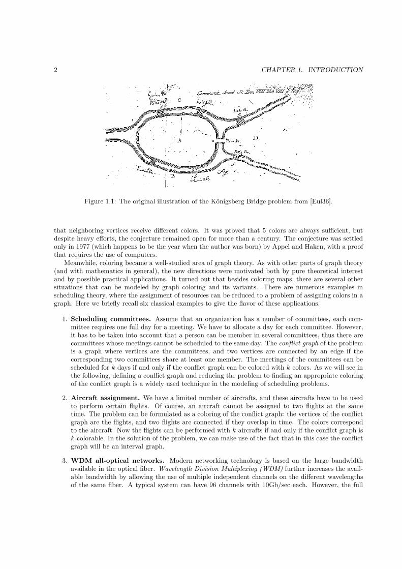
The birth of graph theory is usually attributed to Leonhard Euler’s solution of the Konigsberg Bridgeproblem. The citizens of Konigsberg (now Kaliningrad, Russia) asked the famous mathematician whetherit is possible to visit all the bridges of the city in such a way that we go through every bridge exactlyonce. Euler observed that if such a walk exists, then there can be at most two land masses (the islandsand the two banks of the river Pregel) that have odd number of bridges. There were more than two suchislands in Konigsberg (see Figure 1.1), hence he concluded that it is not possible to have a walk thatvisits each bridge exactly once. Possibly this negative answer made the citizens disappointed, but theargument opened a new chapter in mathematics. In order to answer the question, Euler reasoned aboutobjects (land masses in this case) and connections between objects (bridges). This is precisely the notionof graph, hence graph theory was born.
Graph theory opened a treasure trove of deep questions and results. There seems to be an unstoppableflow of interesting questions about graphs. Some of these questions were investigated because they appearto be very fundamental and natural (in the mathematical sense), or follow naturally from earlier results.Moreover, this new paradigm of “objects” and “connections” turned out to be a very powerful tool inmodeling a wide range of real-life problems. For example, the German physicist Kirchhoff analyzedelectrical circuits using graphs. Roads, railways, and other transportation networks can be describedas graphs. More recently, computer networks and the internet offer a particularly good example wheregraph-theoretic concepts and methods can be used successfully to solve real-life engineering problems.But graphs are useful not only in situations involving network-like physical structures, they can be usedto model more abstract problems. For example, graphs hold the key to the solution in such diverseapplication areas as optimizing register allocations in compilers or reassembling DNA fragments.
Graph coloring is one of the earliest areas of graph theory. It was motivated by the famous Four ColorConjecture. Map makers in the nineteenth century observed that apparently every planar map can becolored using four colors in such a way that countries sharing a boundary have different colors. In thelanguage of graph theory, the conjecture says that every planar graph can be colored with 4 colors such
2 CHAPTER 1. INTRODUCTION
Figure 1.1: The original illustration of the Konigsberg Bridge problem from [Eul36].
that neighboring vertices receive different colors. It was proved that 5 colors are always sufficient, butdespite heavy efforts, the conjecture remained open for more than a century. The conjecture was settledonly in 1977 (which happens to be the year when the author was born) by Appel and Haken, with a proofthat requires the use of computers.
Meanwhile, coloring became a well-studied area of graph theory. As with other parts of graph theory(and with mathematics in general), the new directions were motivated both by pure theoretical interestand by possible practical applications. It turned out that besides coloring maps, there are several othersituations that can be modeled by graph coloring and its variants. There are numerous examples inscheduling theory, where the assignment of resources can be reduced to a problem of assigning colors in agraph. Here we briefly recall six classical examples to give the flavor of these applications.
1. Scheduling committees. Assume that an organization has a number of committees, each com-mittee requires one full day for a meeting. We have to allocate a day for each committee. However,it has to be taken into account that a person can be member in several committees, thus there arecommittees whose meetings cannot be scheduled to the same day. The conflict graph of the problemis a graph where vertices are the committees, and two vertices are connected by an edge if thecorresponding two committees share at least one member. The meetings of the committees can bescheduled for k days if and only if the conflict graph can be colored with k colors. As we will see inthe following, defining a conflict graph and reducing the problem to finding an appropriate coloringof the conflict graph is a widely used technique in the modeling of scheduling problems.
2. Aircraft assignment. We have a limited number of aircrafts, and these aircrafts have to be usedto perform certain flights. Of course, an aircraft cannot be assigned to two flights at the sametime. The problem can be formulated as a coloring of the conflict graph: the vertices of the conflictgraph are the flights, and two flights are connected if they overlap in time. The colors correspondto the aircraft. Now the flights can be performed with k aircrafts if and only if the conflict graph isk-colorable. In the solution of the problem, we can make use of the fact that in this case the conflictgraph will be an interval graph.
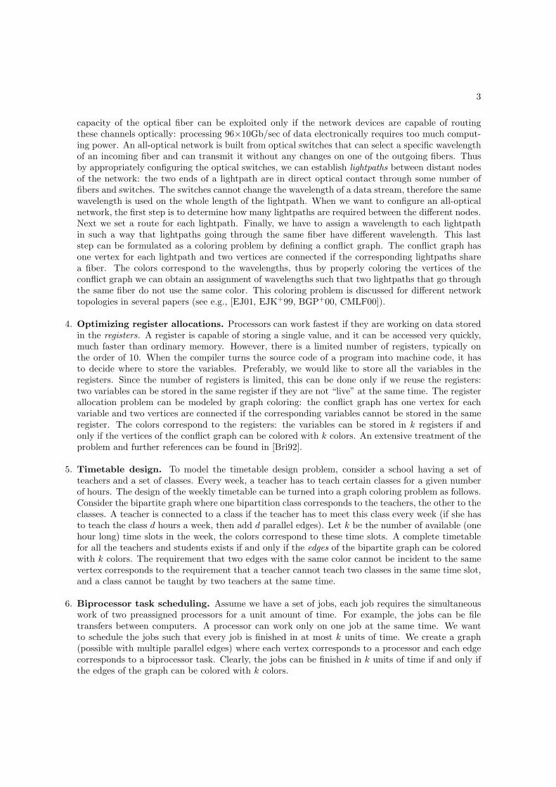
3. WDM all-optical networks. Modern networking technology is based on the large bandwidthavailable in the optical fiber. Wavelength Division Multiplexing (WDM) further increases the avail-able bandwidth by allowing the use of multiple independent channels on the different wavelengthsof the same fiber. A typical system can have 96 channels with 10Gb/sec each. However, the full
3
capacity of the optical fiber can be exploited only if the network devices are capable of routingthese channels optically: processing 96×10Gb/sec of data electronically requires too much comput-ing power. An all-optical network is built from optical switches that can select a specific wavelengthof an incoming fiber and can transmit it without any changes on one of the outgoing fibers. Thusby appropriately configuring the optical switches, we can establish lightpaths between distant nodesof the network: the two ends of a lightpath are in direct optical contact through some number offibers and switches. The switches cannot change the wavelength of a data stream, therefore the samewavelength is used on the whole length of the lightpath. When we want to configure an all-opticalnetwork, the first step is to determine how many lightpaths are required between the different nodes.Next we set a route for each lightpath. Finally, we have to assign a wavelength to each lightpathin such a way that lightpaths going through the same fiber have different wavelength. This laststep can be formulated as a coloring problem by defining a conflict graph. The conflict graph hasone vertex for each lightpath and two vertices are connected if the corresponding lightpaths sharea fiber. The colors correspond to the wavelengths, thus by properly coloring the vertices of theconflict graph we can obtain an assignment of wavelengths such that two lightpaths that go throughthe same fiber do not use the same color. This coloring problem is discussed for different networktopologies in several papers (see e.g., [EJ01, EJK+99, BGP+00, CMLF00]).
4. Optimizing register allocations. Processors can work fastest if they are working on data storedin the registers. A register is capable of storing a single value, and it can be accessed very quickly,much faster than ordinary memory. However, there is a limited number of registers, typically onthe order of 10. When the compiler turns the source code of a program into machine code, it hasto decide where to store the variables. Preferably, we would like to store all the variables in theregisters. Since the number of registers is limited, this can be done only if we reuse the registers:two variables can be stored in the same register if they are not “live” at the same time. The registerallocation problem can be modeled by graph coloring: the conflict graph has one vertex for eachvariable and two vertices are connected if the corresponding variables cannot be stored in the sameregister. The colors correspond to the registers: the variables can be stored in k registers if andonly if the vertices of the conflict graph can be colored with k colors. An extensive treatment of theproblem and further references can be found in [Bri92].
5. Timetable design. To model the timetable design problem, consider a school having a set ofteachers and a set of classes. Every week, a teacher has to teach certain classes for a given numberof hours. The design of the weekly timetable can be turned into a graph coloring problem as follows.Consider the bipartite graph where one bipartition class corresponds to the teachers, the other to theclasses. A teacher is connected to a class if the teacher has to meet this class every week (if she hasto teach the class d hours a week, then add d parallel edges). Let k be the number of available (onehour long) time slots in the week, the colors correspond to these time slots. A complete timetablefor all the teachers and students exists if and only if the edges of the bipartite graph can be coloredwith k colors. The requirement that two edges with the same color cannot be incident to the samevertex corresponds to the requirement that a teacher cannot teach two classes in the same time slot,and a class cannot be taught by two teachers at the same time.
6. Biprocessor task scheduling. Assume we have a set of jobs, each job requires the simultaneouswork of two preassigned processors for a unit amount of time. For example, the jobs can be filetransfers between computers. A processor can work only on one job at the same time. We wantto schedule the jobs such that every job is finished in at most k units of time. We create a graph(possible with multiple parallel edges) where each vertex corresponds to a processor and each edgecorresponds to a biprocessor task. Clearly, the jobs can be finished in k units of time if and only ifthe edges of the graph can be colored with k colors.
4 CHAPTER 1. INTRODUCTION
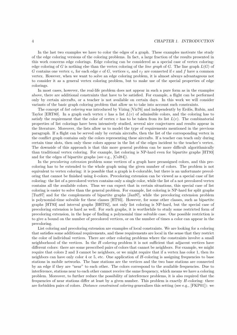
In the last two examples we have to color the edges of a graph. These examples motivate the studyof the edge coloring versions of the coloring problems. In fact, a large fraction of the results presented inthis work concerns edge colorings. Edge coloring can be considered as a special case of vertex coloring:edge coloring of G is nothing else than the vertex coloring of the line graph of G. The line graph L(G) ofG contains one vertex ve for each edge e of G, vertices ve and vf are connected if e and f have a commonvertex. However, when we want to solve an edge coloring problem, it is almost always advantageous notto consider it as a general vertex coloring problem, but to make use of the special properties of edgecolorings.
In most cases, however, the real-life problem does not appear in such a pure form as in the examplesabove, there are additional constraints that have to be satisfied. For example, a flight can be performedonly by certain aircrafts, or a teacher is not available on certain days. In this work we will considervariants of the basic graph coloring problem that allow us to take into account such constraints.
The concept of list coloring was introduced by Vizing [Viz76] and independently by Erdos, Rubin, andTaylor [ERT80]. In a graph each vertex v has a list L(v) of admissible colors, and the coloring has tosatisfy the requirement that the color of vertex v has to be taken from its list L(v). The combinatorialproperties of list colorings have been intensively studied, several nice conjectures and results appear inthe literature. Moreover, the lists allow us to model the type of requirements mentioned in the previousparagraph. If a flight can be served only by certain aircrafts, then the list of the corresponding vertex inthe conflict graph contains only the colors representing these aircrafts. If a teacher can teach only duringcertain time slots, then only these colors appear in the list of the edges incident to the teacher’s vertex.The downside of this approach is that this more general problem can be more difficult algorithmicallythan traditional vertex coloring. For example, list coloring is NP-hard even for bipartite graphs [HT93]and for the edges of bipartite graphs (see e.g., [Col84]).
In the precoloring extension problem some vertices of a graph have preassigned colors, and this pre-coloring has to be extended to the whole graph using the given number of colors. The problem is notequivalent to vertex coloring: it is possible that a graph is k-colorable, but there is an unfortunate precol-oring that cannot be finished using k-colors. Precoloring extension can be viewed as a special case of listcoloring: the list of a precolored vertex contains only a single color, while the list of a not precolored vertexcontains all the available colors. Thus we can expect that in certain situations, this special case of listcoloring is easier to solve than the general problem. For example, list coloring is NP-hard for split graphs[Tuz97] and for the complements of bipartite graphs [Jan97], while the precoloring extension problemis polynomial-time solvable for these classes [HT93]. However, for some other classes, such as bipartitegraphs [HT93] and interval graphs [BHT92], not only list coloring is NP-hard, but the special case ofprecoloring extension is hard as well. For such graphs, it is worthwhile to study some restricted form ofprecoloring extension, in the hope of finding a polynomial time solvable case. One possible restriction isto give a bound on the number of precolored vertices, or on the number of times a color can appear in theprecoloring.
List coloring and precoloring extension are examples of local constraints. We are looking for a coloringthat satisfies some additional requirements, and these requirements are local in the sense that they restrictthe color of individual vertices. There are other coloring problems where the constraints involve a smallneighborhood of the vertices. In the H-coloring problem it is not sufficient that adjacent vertices havedifferent colors: there are some prescribed pairs of colors that cannot be neighbors. For example, we mightrequire that colors 2 and 3 cannot be neighbors, or we might require that if a vertex has color 1, then itsneighbors can have only color 4 or 5, etc. One application of H-coloring is assigning frequencies to basestations in mobile networks. The base stations are the vertices and the two base stations are connectedby an edge if they are “near” to each other. The colors correspond to the available frequencies. Due tointerference, stations near to each other cannot receive the same frequency, which means we have a coloringproblem. Moreover, to further reduce the possibility of interference problems, it is also required that thefrequencies of near stations differ at least by a given number. This problem is exactly H-coloring: thereare forbidden pairs of colors. Distance constrained coloring generalizes this setting (see e.g., [FKP01]): we
5
have two parameters p, q, now the requirement is that the colors of neighboring vertices differ by at leastp, and the colors of vertices at distance 2 differ by at least q. This is also a local requirement: whether acolor is allowed on a vertex or not depends only on the coloring of a small neighborhood of the vertex.
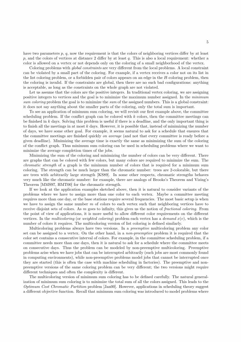
Coloring problems with global constraints are very different from the local problems. A local constraintcan be violated by a small part of the coloring. For example, if a vertex receives a color not on its list inthe list coloring problem, or a forbidden pair of colors appears on an edge in the H-coloring problem, thenthe coloring is invalid. If the constraints are global, then there are no such bad configurations: anythingis acceptable, as long as the constraints on the whole graph are not violated.
Let us assume that the colors are the positive integers. In traditional vertex coloring, we are assigningpositive integers to vertices and the goal is to minimize the maximum number assigned. In the minimumsum coloring problem the goal is to minimize the sum of the assigned numbers. This is a global constraint:it does not say anything about the smaller parts of the coloring, only the total sum is important.
To see an application of minimum sum coloring, we will revisit our first example above, the committeescheduling problem. If the conflict graph can be colored with k colors, then the committee meetings canbe finished in k days. Solving this problem is useful if there is a deadline, and the only important thing isto finish all the meetings in at most k days. However, it is possible that, instead of minimizing the numberof days, we have some other goal. For example, it seems natural to ask for a schedule that ensures thatthe committee meetings are finished quickly on average (and not that every committee is ready before agiven deadline). Minimizing the average time is exactly the same as minimizing the sum of the coloringof the conflict graph. Thus minimum sum coloring can be used in scheduling problems where we want tominimize the average completion times of the jobs.
Minimizing the sum of the coloring and minimizing the number of colors can be very different. Thereare graphs that can be colored with few colors, but many colors are required to minimize the sum. Thechromatic strength of a graph is the minimum number of colors that is required for a minimum sumcoloring. The strength can be much larger than the chromatic number: trees are 2-colorable, but thereare trees with arbitrarily large strength [KS89]. In some other respects, chromatic strengths behavesvery much like the chromatic number: for example, there are analogs of Brooks’s Theorem and Vizing’sTheorem [MMS97, HMT00] for the chromatic strength.
If we look at the application examples sketched above, then it is natural to consider variants of theproblems where we have to assign more than one color to each vertex. Maybe a committee meetingrequires more than one day, or the base stations require several frequencies. The most basic setup is whenwe have to assign the same number m of colors to each vertex such that neighboring vertices have toreceive disjoint sets of colors. As m goes to infinity, this gives us the notion of fractional coloring. Fromthe point of view of applications, it is more useful to allow different color requirements on the differentvertices. In the multicoloring (or weighted coloring) problem each vertex has a demand x(v), which is thenumber of colors it requires. The multicoloring version of list coloring is defined similarly.
Multicoloring problems always have two versions. In a preemptive multicoloring problem any colorset can be assigned to a vertex. On the other hand, in a non-preemptive problem it is required that thecolor set contains a consecutive interval of colors. For example, in the committee scheduling problem, if acommittee needs more than one days, then it is natural to ask for a schedule where the committee meetson consecutive days. Thus the problem can be modeled by non-preemptive multicoloring. Preemptiveproblems arise when we have jobs that can be interrupted arbitrarily (such jobs are most commonly foundin computing environments), while non-preemptive problems model jobs that cannot be interrupted oncethey are started (this is often the case with machine scheduling in factories). The preemptive and non-preemptive versions of the same coloring problem can be very different; the two versions might requiredifferent techniques and often the complexity is different.
The multicoloring version of minimum sum coloring has to be defined carefully. The natural general-ization of minimum sum coloring is to minimize the total sum of all the colors assigned. This leads to theOptimum Cost Chromatic Partition problem [Jan00]. However, applications in scheduling theory suggesta different objective function. Recall that minimum sum coloring was introduced to model problems where
6 CHAPTER 1. INTRODUCTION
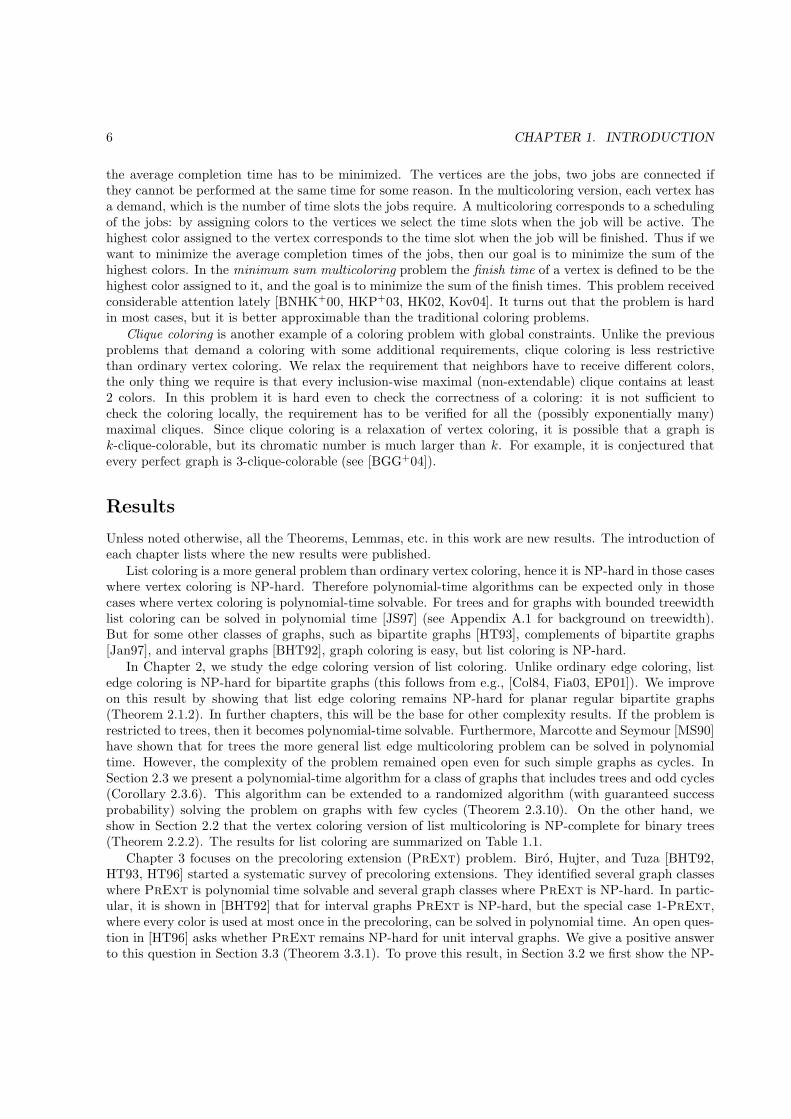
the average completion time has to be minimized. The vertices are the jobs, two jobs are connected ifthey cannot be performed at the same time for some reason. In the multicoloring version, each vertex hasa demand, which is the number of time slots the jobs require. A multicoloring corresponds to a schedulingof the jobs: by assigning colors to the vertices we select the time slots when the job will be active. Thehighest color assigned to the vertex corresponds to the time slot when the job will be finished. Thus if wewant to minimize the average completion times of the jobs, then our goal is to minimize the sum of thehighest colors. In the minimum sum multicoloring problem the finish time of a vertex is defined to be thehighest color assigned to it, and the goal is to minimize the sum of the finish times. This problem receivedconsiderable attention lately [BNHK+00, HKP+03, HK02, Kov04]. It turns out that the problem is hardin most cases, but it is better approximable than the traditional coloring problems.
Clique coloring is another example of a coloring problem with global constraints. Unlike the previousproblems that demand a coloring with some additional requirements, clique coloring is less restrictivethan ordinary vertex coloring. We relax the requirement that neighbors have to receive different colors,the only thing we require is that every inclusion-wise maximal (non-extendable) clique contains at least2 colors. In this problem it is hard even to check the correctness of a coloring: it is not sufficient tocheck the coloring locally, the requirement has to be verified for all the (possibly exponentially many)maximal cliques. Since clique coloring is a relaxation of vertex coloring, it is possible that a graph isk-clique-colorable, but its chromatic number is much larger than k. For example, it is conjectured thatevery perfect graph is 3-clique-colorable (see [BGG+04]).
Results
Unless noted otherwise, all the Theorems, Lemmas, etc. in this work are new results. The introduction ofeach chapter lists where the new results were published.
List coloring is a more general problem than ordinary vertex coloring, hence it is NP-hard in those caseswhere vertex coloring is NP-hard. Therefore polynomial-time algorithms can be expected only in thosecases where vertex coloring is polynomial-time solvable. For trees and for graphs with bounded treewidthlist coloring can be solved in polynomial time [JS97] (see Appendix A.1 for background on treewidth).But for some other classes of graphs, such as bipartite graphs [HT93], complements of bipartite graphs[Jan97], and interval graphs [BHT92], graph coloring is easy, but list coloring is NP-hard.
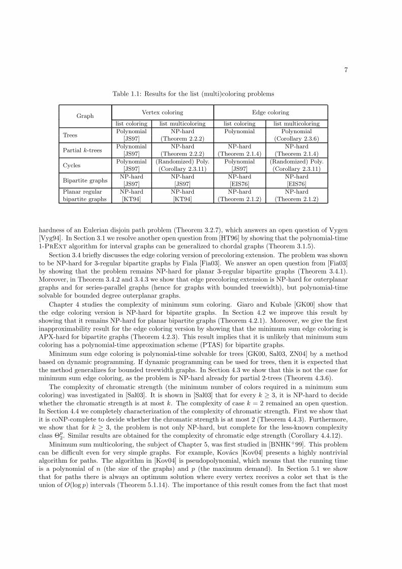
In Chapter 2, we study the edge coloring version of list coloring. Unlike ordinary edge coloring, listedge coloring is NP-hard for bipartite graphs (this follows from e.g., [Col84, Fia03, EP01]). We improveon this result by showing that list edge coloring remains NP-hard for planar regular bipartite graphs(Theorem 2.1.2). In further chapters, this will be the base for other complexity results. If the problem isrestricted to trees, then it becomes polynomial-time solvable. Furthermore, Marcotte and Seymour [MS90]have shown that for trees the more general list edge multicoloring problem can be solved in polynomialtime. However, the complexity of the problem remained open even for such simple graphs as cycles. InSection 2.3 we present a polynomial-time algorithm for a class of graphs that includes trees and odd cycles(Corollary 2.3.6). This algorithm can be extended to a randomized algorithm (with guaranteed successprobability) solving the problem on graphs with few cycles (Theorem 2.3.10). On the other hand, weshow in Section 2.2 that the vertex coloring version of list multicoloring is NP-complete for binary trees(Theorem 2.2.2). The results for list coloring are summarized on Table 1.1.
Chapter 3 focuses on the precoloring extension (PrExt) problem. Biro, Hujter, and Tuza [BHT92,HT93, HT96] started a systematic survey of precoloring extensions. They identified several graph classeswhere PrExt is polynomial time solvable and several graph classes where PrExt is NP-hard. In partic-ular, it is shown in [BHT92] that for interval graphs PrExt is NP-hard, but the special case 1-PrExt,where every color is used at most once in the precoloring, can be solved in polynomial time. An open ques-tion in [HT96] asks whether PrExt remains NP-hard for unit interval graphs. We give a positive answerto this question in Section 3.3 (Theorem 3.3.1). To prove this result, in Section 3.2 we first show the NP-
7
Table 1.1: Results for the list (multi)coloring problems
Vertex coloring Edge coloringGraph
list coloring list multicoloring list coloring list multicoloring
TreesPolynomial NP-hard Polynomial Polynomial
[JS97] (Theorem 2.2.2) (Corollary 2.3.6)
Partial k-treesPolynomial NP-hard NP-hard NP-hard
[JS97] (Theorem 2.2.2) (Theorem 2.1.4) (Theorem 2.1.4)
CyclesPolynomial (Randomized) Poly. Polynomial (Randomized) Poly.
[JS97] (Corollary 2.3.11) [JS97] (Corollary 2.3.11)
Bipartite graphsNP-hard NP-hard NP-hard NP-hard[JS97] [JS97] [EIS76] [EIS76]
Planar regular NP-hard NP-hard NP-hard NP-hardbipartite graphs [KT94] [KT94] (Theorem 2.1.2) (Theorem 2.1.2)
hardness of an Eulerian disjoin path problem (Theorem 3.2.7), which answers an open question of Vygen[Vyg94]. In Section 3.1 we resolve another open question from [HT96] by showing that the polynomial-time1-PrExt algorithm for interval graphs can be generalized to chordal graphs (Theorem 3.1.5).
Section 3.4 briefly discusses the edge coloring version of precoloring extension. The problem was shownto be NP-hard for 3-regular bipartite graphs by Fiala [Fia03]. We answer an open question from [Fia03]by showing that the problem remains NP-hard for planar 3-regular bipartite graphs (Theorem 3.4.1).Moreover, in Theorem 3.4.2 and 3.4.3 we show that edge precoloring extension is NP-hard for outerplanargraphs and for series-parallel graphs (hence for graphs with bounded treewidth), but polynomial-timesolvable for bounded degree outerplanar graphs.
Chapter 4 studies the complexity of minimum sum coloring. Giaro and Kubale [GK00] show thatthe edge coloring version is NP-hard for bipartite graphs. In Section 4.2 we improve this result byshowing that it remains NP-hard for planar bipartite graphs (Theorem 4.2.1). Moreover, we give the firstinapproximability result for the edge coloring version by showing that the minimum sum edge coloring isAPX-hard for bipartite graphs (Theorem 4.2.3). This result implies that it is unlikely that minimum sumcoloring has a polynomial-time approximation scheme (PTAS) for bipartite graphs.
Minimum sum edge coloring is polynomial-time solvable for trees [GK00, Sal03, ZN04] by a methodbased on dynamic programming. If dynamic programming can be used for trees, then it is expected thatthe method generalizes for bounded treewidth graphs. In Section 4.3 we show that this is not the case forminimum sum edge coloring, as the problem is NP-hard already for partial 2-trees (Theorem 4.3.6).
The complexity of chromatic strength (the minimum number of colors required in a minimum sumcoloring) was investigated in [Sal03]. It is shown in [Sal03] that for every k ≥ 3, it is NP-hard to decidewhether the chromatic strength is at most k. The complexity of case k = 2 remained an open question.In Section 4.4 we completely characterization of the complexity of chromatic strength. First we show thatit is coNP-complete to decide whether the chromatic strength is at most 2 (Theorem 4.4.3). Furthermore,we show that for k ≥ 3, the problem is not only NP-hard, but complete for the less-known complexityclass Θp
2. Similar results are obtained for the complexity of chromatic edge strength (Corollary 4.4.12).
Minimum sum multicoloring, the subject of Chapter 5, was first studied in [BNHK+99]. This problemcan be difficult even for very simple graphs. For example, Kovacs [Kov04] presents a highly nontrivialalgorithm for paths. The algorithm in [Kov04] is pseudopolynomial, which means that the running timeis a polynomial of n (the size of the graphs) and p (the maximum demand). In Section 5.1 we showthat for paths there is always an optimum solution where every vertex receives a color set that is theunion of O(log p) intervals (Theorem 5.1.14). The importance of this result comes from the fact that most
8 CHAPTER 1. INTRODUCTION
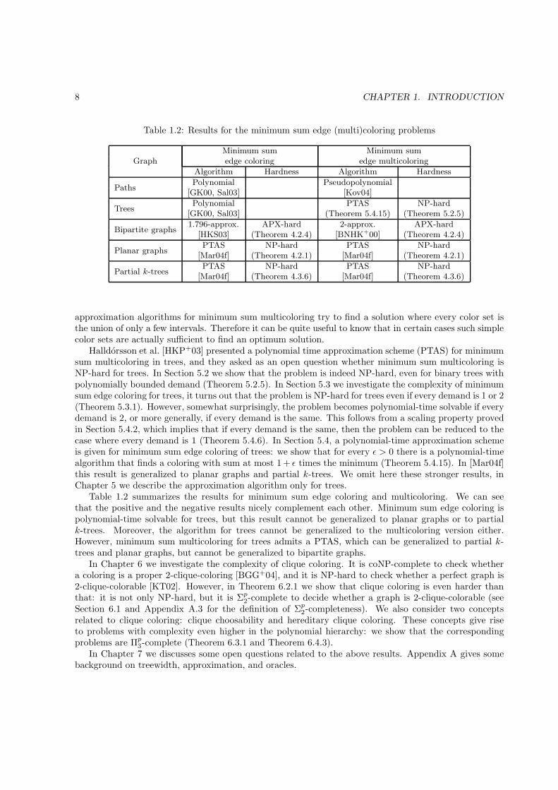
Table 1.2: Results for the minimum sum edge (multi)coloring problems
Minimum sum Minimum sumGraph edge coloring edge multicoloring
Algorithm Hardness Algorithm Hardness
PathsPolynomial Pseudopolynomial
[GK00, Sal03] [Kov04]
TreesPolynomial PTAS NP-hard
[GK00, Sal03] (Theorem 5.4.15) (Theorem 5.2.5)
Bipartite graphs1.796-approx. APX-hard 2-approx. APX-hard
[HKS03] (Theorem 4.2.4) [BNHK+00] (Theorem 4.2.4)
Planar graphsPTAS NP-hard PTAS NP-hard
[Mar04f] (Theorem 4.2.1) [Mar04f] (Theorem 4.2.1)
Partial k-treesPTAS NP-hard PTAS NP-hard
[Mar04f] (Theorem 4.3.6) [Mar04f] (Theorem 4.3.6)
approximation algorithms for minimum sum multicoloring try to find a solution where every color set isthe union of only a few intervals. Therefore it can be quite useful to know that in certain cases such simplecolor sets are actually sufficient to find an optimum solution.
Halldorsson et al. [HKP+03] presented a polynomial time approximation scheme (PTAS) for minimumsum multicoloring in trees, and they asked as an open question whether minimum sum multicoloring isNP-hard for trees. In Section 5.2 we show that the problem is indeed NP-hard, even for binary trees withpolynomially bounded demand (Theorem 5.2.5). In Section 5.3 we investigate the complexity of minimumsum edge coloring for trees, it turns out that the problem is NP-hard for trees even if every demand is 1 or 2(Theorem 5.3.1). However, somewhat surprisingly, the problem becomes polynomial-time solvable if everydemand is 2, or more generally, if every demand is the same. This follows from a scaling property provedin Section 5.4.2, which implies that if every demand is the same, then the problem can be reduced to thecase where every demand is 1 (Theorem 5.4.6). In Section 5.4, a polynomial-time approximation schemeis given for minimum sum edge coloring of trees: we show that for every ǫ > 0 there is a polynomial-timealgorithm that finds a coloring with sum at most 1 + ǫ times the minimum (Theorem 5.4.15). In [Mar04f]this result is generalized to planar graphs and partial k-trees. We omit here these stronger results, inChapter 5 we describe the approximation algorithm only for trees.
Table 1.2 summarizes the results for minimum sum edge coloring and multicoloring. We can seethat the positive and the negative results nicely complement each other. Minimum sum edge coloring ispolynomial-time solvable for trees, but this result cannot be generalized to planar graphs or to partialk-trees. Moreover, the algorithm for trees cannot be generalized to the multicoloring version either.However, minimum sum multicoloring for trees admits a PTAS, which can be generalized to partial k-trees and planar graphs, but cannot be generalized to bipartite graphs.
In Chapter 6 we investigate the complexity of clique coloring. It is coNP-complete to check whethera coloring is a proper 2-clique-coloring [BGG+04], and it is NP-hard to check whether a perfect graph is2-clique-colorable [KT02]. However, in Theorem 6.2.1 we show that clique coloring is even harder thanthat: it is not only NP-hard, but it is Σp2-complete to decide whether a graph is 2-clique-colorable (seeSection 6.1 and Appendix A.3 for the definition of Σp2-completeness). We also consider two conceptsrelated to clique coloring: clique choosability and hereditary clique coloring. These concepts give riseto problems with complexity even higher in the polynomial hierarchy: we show that the correspondingproblems are Πp
3-complete (Theorem 6.3.1 and Theorem 6.4.3).In Chapter 7 we discusses some open questions related to the above results. Appendix A gives some
background on treewidth, approximation, and oracles.
CHAPTER 2
List coloring
People can have the Model T in any color—so long as it’s black.Henry Ford (1863–1947)
The concept of list coloring was introduced independently by Vizing [Viz76] and by Erdos, Rubin, andTaylor [ERT80]. Given a graph G(V,E), a list assignment L is a function that assigns to each vertex v ∈ Va set of admissible colors L(v). The list assignment is called a k-assignment if |L(v)| = k for every v ∈ V .Graph G is L-colorable if there is a coloring ψ of the vertices such that ψ(v) ∈ L(v), and ψ(u) 6= ψ(v)whenever u and v are neighbors.
Much of the research done on list coloring concerns the notion of choosability. A graph G is k-choosableif it has an L-coloring for every k-assignment L. The list chromatic number of a graph is k if the graphis k-choosable but not (k − 1)-choosable. It is obvious that the list chromatic number cannot be smallerthan the chromatic number. On the other hand, there can be an arbitrarily large gap between the twoparameters: for example, there are bipartite graphs with arbitrarily large list chromatic number [ERT80].There are several deep results and conjectures in the literature on the combinatorial properties of the listchromatic number. However, here we approach list coloring from the algorithmic and complexity theoreticpoint of view. Choosability will be considered only in Section 6, in the context of clique colorings.
List coloring, being a generalization of vertex coloring, is NP-complete on every class of graphs wherevertex coloring is NP-complete. Furthermore, there are cases where vertex coloring is easy, but listcoloring is hard. For example, list coloring is NP-hard for bipartite graphs [HT93], complements ofbipartite graphs [Jan97], and interval graphs [BHT92], while there are efficient coloring algorithms forthese classes of perfect graphs. There are very few cases where list coloring is polynomial time solvable:it can be solved in linear time for trees, and more generally, for partial k-trees [JS97]. Moreover, if everylist contains at most 2 colors, then the problem can be solved in linear time by a reduction to 2SAT.
In this chapter we consider the edge coloring version of list coloring. Ordinary edge coloring is NP-hard[Hol81, LG83], but can be solved in polynomial time for bipartite graphs. In fact, Konig’s Line ColoringTheorem states that the edges of a bipartite graph can be colored with k colors if and only if the maximumdegree is at most k. On the other hand, as observed in [Kub93], it follows from an old result of Even,Itai, and Shamir [EIS76] on the timetable problem that list edge coloring is NP-hard for bipartite graphswith maximum degree 3. In Section 2.1.1 we strengthen this result by showing that the problem remainsNP-hard for planar, 3-regular bipartite graphs.
10 CHAPTER 2. LIST COLORING
In [FZN03, FIZN03, JMT99, Wu00] the list edge coloring problem is considered for series-parallelgraphs, sufficient conditions are given for some special cases. In Section 2.1.2 we investigate the com-putational complexity of the problem. An easy argument shows that list edge coloring can be solved inpolynomial time for bounded degree series-parallel graphs. However, we prove that the problem becomesNP-hard for series-parallel graphs if the maximum degree can be arbitrary. The same results hold forouterplanar graphs as well.
Using a method that combines dynamic programming and matching, list edge coloring can be solvedin polynomial time for trees [Tuz97]. However, unlike in the vertex coloring case, this approach cannot begeneralized to partial k-trees: outerplanar and series-parallel graphs have treewidth at most 2, thus theresults mentioned in the previous paragraph show that list edge coloring is NP-complete for partial 2-trees(see Appendix A.1 for the definition of treewidth and partial k-trees). This is somewhat surprising, sincethere are very few problems that are polynomial time solvable for trees but NP-hard for partial 2-trees.Usually it is expected that if a dynamic programming approach works for trees, then it can be generalizedto partial k-trees. Another recent example where the problem is easy for trees but NP-hard for partial2-trees is the edge disjoint paths problem [NVZ01].
In the list multicoloring problem each vertex v has a demand x(v), and we have to assign v a subset Ψ(v)of L(v) that has size x(v). Of course, the color sets assigned to neighboring vertices have to be disjoint.How does the complexity of the problem changes if we move from list coloring to list multicoloring? Is itpossible to generalize the polynomial-time solvable cases of list coloring to the multicoloring problem? InSection 2.2 we show that list multicoloring is NP-hard for binary trees, thus the dynamic programmingmethod for trees and for partial k-trees cannot be generalized to the multicoloring case. On the otherhand, Marcotte and Seymour [MS90] proved a good characterization theorem for list edge multicoloringof trees. The proof can be turned into a polynomial-time algorithm for the list edge multicoloring oftrees. In Section 2.3, we give a polynomial-time algorithm for a slightly more general class of graphs,which includes odd cycles, for example. With some further work, the algorithm can be extended to arandomized polynomial-time algorithm that works for graphs that have only a constant number of cycles.Randomized algorithm here means that the algorithm uses random numbers, and depending on the randomnumbers, there is a small constant probability that the result is wrong. However, this probability can bemade arbitrarily small by repeating the algorithm multiple times.
Section 2.1 will appear as part of [Mar04i]. The results in Section 2.2 are taken from [Mar02]. Sec-tion 2.3 contains the results of [Mar03a] and in [Mar04e].
2.1 List edge coloring planar graphs
In this section we prove that list edge coloring is NP-complete restricted to various classes of planar graphs.Formally, we study the following problem:
List edge coloring
Input: A graph G(V,E), a set of colors C and a color list L: E → 2C for each edge.
Question: Is there an edge coloring ψ: E → C such that
• ψ(e) ∈ L(e) for every e ∈ E, and
• ψ(e1) 6= ψ(e2) if e1 and e2 are incident to the same vertex in G?
Section 2.1.1 shows that the problem is NP-complete for planar 3-regular bipartite graphs. Section 2.1.2shows that the problem is NP-complete for outerplanar and series-parallel graphs.
2.1. LIST EDGE COLORING PLANAR GRAPHS 11
C1 2323
23
313131
12
12
121212
12D1 B1
A1
B3
D3
C2
D2
A2
B2
A3
C3
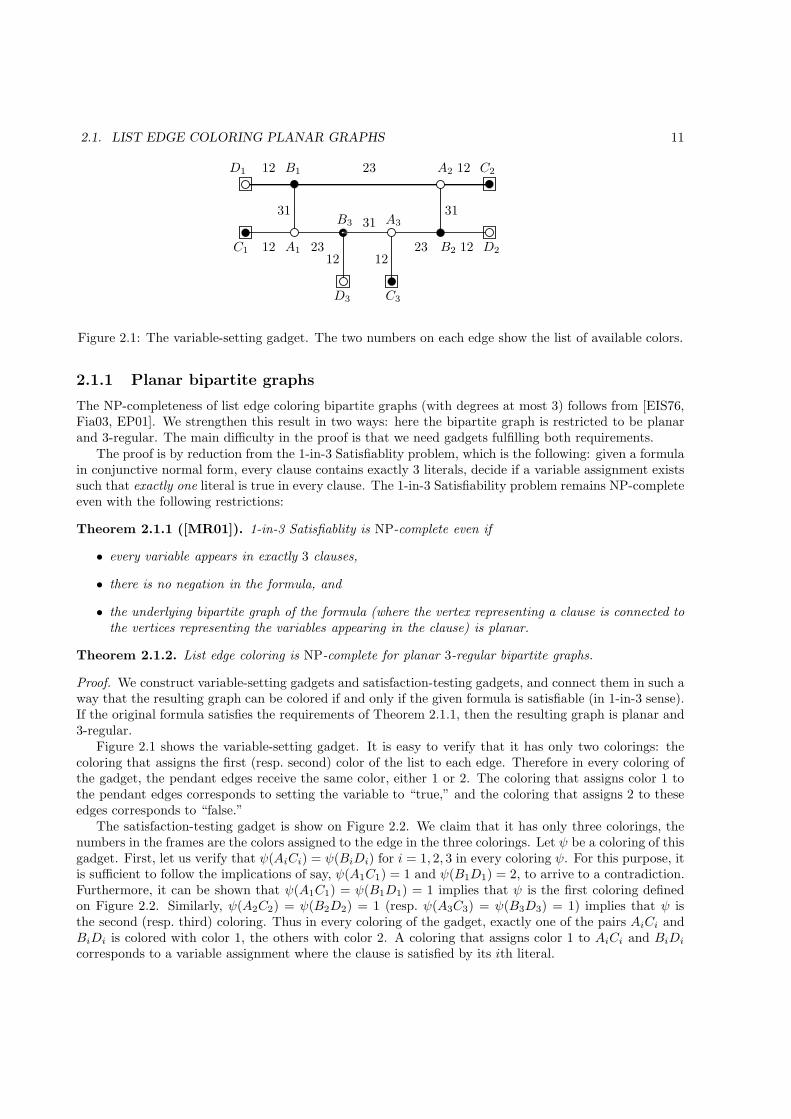
Figure 2.1: The variable-setting gadget. The two numbers on each edge show the list of available colors.
2.1.1 Planar bipartite graphs
The NP-completeness of list edge coloring bipartite graphs (with degrees at most 3) follows from [EIS76,Fia03, EP01]. We strengthen this result in two ways: here the bipartite graph is restricted to be planarand 3-regular. The main difficulty in the proof is that we need gadgets fulfilling both requirements.
The proof is by reduction from the 1-in-3 Satisfiablity problem, which is the following: given a formulain conjunctive normal form, every clause contains exactly 3 literals, decide if a variable assignment existssuch that exactly one literal is true in every clause. The 1-in-3 Satisfiability problem remains NP-completeeven with the following restrictions:
Theorem 2.1.1 ([MR01]). 1-in-3 Satisfiablity is NP-complete even if
• every variable appears in exactly 3 clauses,
• there is no negation in the formula, and
• the underlying bipartite graph of the formula (where the vertex representing a clause is connected tothe vertices representing the variables appearing in the clause) is planar.
Theorem 2.1.2. List edge coloring is NP-complete for planar 3-regular bipartite graphs.
Proof. We construct variable-setting gadgets and satisfaction-testing gadgets, and connect them in such away that the resulting graph can be colored if and only if the given formula is satisfiable (in 1-in-3 sense).If the original formula satisfies the requirements of Theorem 2.1.1, then the resulting graph is planar and3-regular.
Figure 2.1 shows the variable-setting gadget. It is easy to verify that it has only two colorings: thecoloring that assigns the first (resp. second) color of the list to each edge. Therefore in every coloring ofthe gadget, the pendant edges receive the same color, either 1 or 2. The coloring that assigns color 1 tothe pendant edges corresponds to setting the variable to “true,” and the coloring that assigns 2 to theseedges corresponds to “false.”
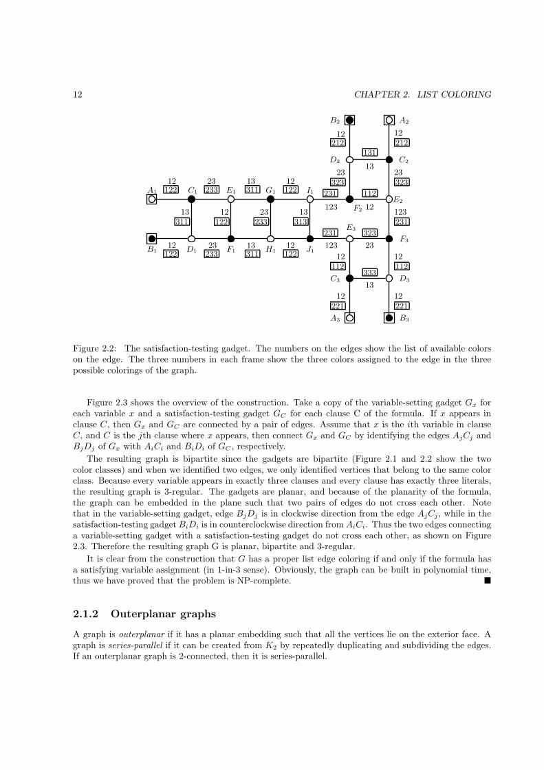
The satisfaction-testing gadget is show on Figure 2.2. We claim that it has only three colorings, thenumbers in the frames are the colors assigned to the edge in the three colorings. Let ψ be a coloring of thisgadget. First, let us verify that ψ(AiCi) = ψ(BiDi) for i = 1, 2, 3 in every coloring ψ. For this purpose, itis sufficient to follow the implications of say, ψ(A1C1) = 1 and ψ(B1D1) = 2, to arrive to a contradiction.Furthermore, it can be shown that ψ(A1C1) = ψ(B1D1) = 1 implies that ψ is the first coloring definedon Figure 2.2. Similarly, ψ(A2C2) = ψ(B2D2) = 1 (resp. ψ(A3C3) = ψ(B3D3) = 1) implies that ψ isthe second (resp. third) coloring. Thus in every coloring of the gadget, exactly one of the pairs AiCi andBiDi is colored with color 1, the others with color 2. A coloring that assigns color 1 to AiCi and BiDi
corresponds to a variable assignment where the clause is satisfied by its ith literal.
12 CHAPTER 2. LIST COLORING
313
333C3 D3
112 112
323E3
F3
123
123
231123
231
231
323 323
112
13 13
311233122 122
311233122 122D1 F1B1 H1 J1
I1E1 G1C1A1
1212 1323
311 122 233
B2
F2
D2 C2
A2
12
12
12
12
23
23
12
12
12
2313
13
13
212212131
E212
1212 2323
A3
221
B3
221
Figure 2.2: The satisfaction-testing gadget. The numbers on the edges show the list of available colorson the edge. The three numbers in each frame show the three colors assigned to the edge in the threepossible colorings of the graph.
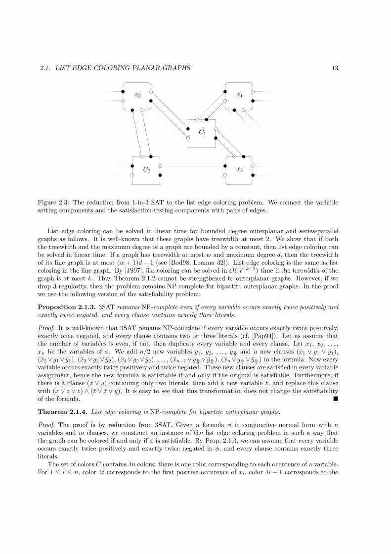
Figure 2.3 shows the overview of the construction. Take a copy of the variable-setting gadget Gx foreach variable x and a satisfaction-testing gadget GC for each clause C of the formula. If x appears inclause C, then Gx and GC are connected by a pair of edges. Assume that x is the ith variable in clauseC, and C is the jth clause where x appears, then connect Gx and GC by identifying the edges AjCj andBjDj of Gx with AiCi and BiDi of GC , respectively.
The resulting graph is bipartite since the gadgets are bipartite (Figure 2.1 and 2.2 show the twocolor classes) and when we identified two edges, we only identified vertices that belong to the same colorclass. Because every variable appears in exactly three clauses and every clause has exactly three literals,the resulting graph is 3-regular. The gadgets are planar, and because of the planarity of the formula,the graph can be embedded in the plane such that two pairs of edges do not cross each other. Notethat in the variable-setting gadget, edge BjDj is in clockwise direction from the edge AjCj , while in thesatisfaction-testing gadgetBiDi is in counterclockwise direction from AiCi. Thus the two edges connectinga variable-setting gadget with a satisfaction-testing gadget do not cross each other, as shown on Figure2.3. Therefore the resulting graph G is planar, bipartite and 3-regular.
It is clear from the construction that G has a proper list edge coloring if and only if the formula hasa satisfying variable assignment (in 1-in-3 sense). Obviously, the graph can be built in polynomial time,thus we have proved that the problem is NP-complete. �
2.1.2 Outerplanar graphs
A graph is outerplanar if it has a planar embedding such that all the vertices lie on the exterior face. Agraph is series-parallel if it can be created from K2 by repeatedly duplicating and subdividing the edges.If an outerplanar graph is 2-connected, then it is series-parallel.
2.1. LIST EDGE COLORING PLANAR GRAPHS 13
x1
C1
C2 x3
x2
Figure 2.3: The reduction from 1-in-3 SAT to the list edge coloring problem. We connect the variablesetting components and the satisfaction-testing components with pairs of edges.
List edge coloring can be solved in linear time for bounded degree outerplanar and series-parallelgraphs as follows. It is well-known that these graphs have treewidth at most 2. We show that if boththe treewidth and the maximum degree of a graph are bounded by a constant, then list edge coloring canbe solved in linear time. If a graph has treewidth at most w and maximum degree d, then the treewidthof its line graph is at most (w + 1)d − 1 (see [Bod98, Lemma 32]). List edge coloring is the same as listcoloring in the line graph. By [JS97], list coloring can be solved in O(|V |k+2) time if the treewidth of thegraph is at most k. Thus Theorem 2.1.2 cannot be strengthened to outerplanar graphs. However, if wedrop 3-regularity, then the problem remains NP-complete for bipartite outerplanar graphs. In the proofwe use the following version of the satisfiability problem:
Proposition 2.1.3. 3SAT remains NP-complete even if every variable occurs exactly twice positively andexactly twice negated, and every clause contains exactly three literals.
Proof. It is well-known that 3SAT remains NP-complete if every variable occurs exactly twice positively,exactly once negated, and every clause contains two or three literals (cf. [Pap94]). Let us assume thatthe number of variables is even, if not, then duplicate every variable and every clause. Let x1, x2, . . . ,xn be the variables of φ. We add n/2 new variables y1, y2, . . . , yn
2and n new clauses (x1 ∨ y1 ∨ y1),
(x2∨y1∨ y1), (x3∨y2∨ y2), (x4∨y2∨ y2), . . . , (xn−1∨yn2∨ yn
2), (xn∨yn
2∨ yn
2) to the formula. Now every
variable occurs exactly twice positively and twice negated. These new clauses are satisfied in every variableassignment, hence the new formula is satisfiable if and only if the original is satisfiable. Furthermore, ifthere is a clause (x ∨ y) containing only two literals, then add a new variable z, and replace this clausewith (x ∨ z ∨ z) ∧ (z ∨ z ∨ y). It is easy to see that this transformation does not change the satisfiabilityof the formula. �
Theorem 2.1.4. List edge coloring is NP-complete for bipartite outerplanar graphs.
Proof. The proof is by reduction from 3SAT. Given a formula φ in conjunctive normal form with nvariables and m clauses, we construct an instance of the list edge coloring problem in such a way thatthe graph can be colored if and only if φ is satisfiable. By Prop. 2.1.3, we can assume that every variableoccurs exactly twice positively and exactly twice negated in φ, and every clause contains exactly threeliterals.
The set of colors C contains 4n colors: there is one color corresponding to each occurence of a variable.For 1 ≤ i ≤ n, color 4i corresponds to the first positive occurence of xi, color 4i − 1 corresponds to the
14 CHAPTER 2. LIST COLORING
{4i−
3, 4i−
1}
{4i−
2,4i}
{4i − 1, 4i − 2}{4i, 4i − 1}{4i, 4i − 3} {4i − 1, 4i}
v
ai bi ci di ei
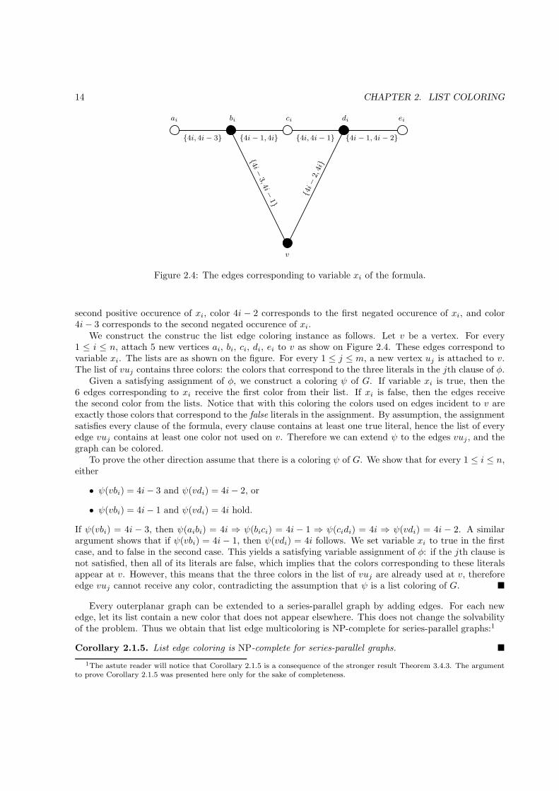
Figure 2.4: The edges corresponding to variable xi of the formula.
second positive occurence of xi, color 4i − 2 corresponds to the first negated occurence of xi, and color4i− 3 corresponds to the second negated occurence of xi.
We construct the construc the list edge coloring instance as follows. Let v be a vertex. For every1 ≤ i ≤ n, attach 5 new vertices ai, bi, ci, di, ei to v as show on Figure 2.4. These edges correspond tovariable xi. The lists are as shown on the figure. For every 1 ≤ j ≤ m, a new vertex uj is attached to v.The list of vuj contains three colors: the colors that correspond to the three literals in the jth clause of φ.
Given a satisfying assignment of φ, we construct a coloring ψ of G. If variable xi is true, then the6 edges corresponding to xi receive the first color from their list. If xi is false, then the edges receivethe second color from the lists. Notice that with this coloring the colors used on edges incident to v areexactly those colors that correspond to the false literals in the assignment. By assumption, the assignmentsatisfies every clause of the formula, every clause contains at least one true literal, hence the list of everyedge vuj contains at least one color not used on v. Therefore we can extend ψ to the edges vuj , and thegraph can be colored.
To prove the other direction assume that there is a coloring ψ of G. We show that for every 1 ≤ i ≤ n,either
• ψ(vbi) = 4i− 3 and ψ(vdi) = 4i− 2, or
• ψ(vbi) = 4i− 1 and ψ(vdi) = 4i hold.
If ψ(vbi) = 4i − 3, then ψ(aibi) = 4i ⇒ ψ(bici) = 4i − 1 ⇒ ψ(cidi) = 4i ⇒ ψ(vdi) = 4i − 2. A similarargument shows that if ψ(vbi) = 4i− 1, then ψ(vdi) = 4i follows. We set variable xi to true in the firstcase, and to false in the second case. This yields a satisfying variable assignment of φ: if the jth clause isnot satisfied, then all of its literals are false, which implies that the colors corresponding to these literalsappear at v. However, this means that the three colors in the list of vuj are already used at v, thereforeedge vuj cannot receive any color, contradicting the assumption that ψ is a list coloring of G. �
Every outerplanar graph can be extended to a series-parallel graph by adding edges. For each newedge, let its list contain a new color that does not appear elsewhere. This does not change the solvabilityof the problem. Thus we obtain that list edge multicoloring is NP-complete for series-parallel graphs:1
Corollary 2.1.5. List edge coloring is NP-complete for series-parallel graphs. �
1The astute reader will notice that Corollary 2.1.5 is a consequence of the stronger result Theorem 3.4.3. The argumentto prove Corollary 2.1.5 was presented here only for the sake of completeness.
2.2. LIST MULTICOLORING OF TREES 15
2.2 List multicoloring of trees
In this section we study the list multicoloring problem, which is defined as follows:
List Multicoloring
Input: A graph G(V,E), a demand function x: V → N, a set of colors C and a color list L:V → 2C for each vertex.
Question: Is there a multicoloring Ψ: V → 2C such that
• Ψ(v) ⊆ L(v) for every v ∈ V ,
• Ψ(u) ∩ Ψ(v) = ∅ if u and v are neighbors in G, and
• |Ψ(v)| = x(v) for every v ∈ V ?
We show that list multicoloring is NP-hard for trees, even if the degree of every node is at most three.But before that we briefly discuss how list coloring can be solved for trees, and why the algorithm for listcoloring cannot be generalized to list multicoloring. We present two algorithms from [JS97, Tuz97], butneither of them works in the case of multicoloring.
Algorithm 1. A list coloring of a tree can be found the following way. First, if there is a vertex v whoselist contains only one color c, then this vertex can be removed from the problem: assign color c to v, deletec from the lists of the neighbors of v, and remove v from the graph. Therefore it can be assumed thatevery list contains at least two colors. We claim that the tree can be colored with the lists. We prove thisby induction on the number of vertices. Let v be a leaf of the tree. Delete v from the tree, the remainingtree can be colored by the induction hypothesis. This coloring assigns some color c to the neighbor ofv. Since the list of v contains at least two colors, thus we can assign to v a color different from v, whichextends the coloring to the whole tree, completing the induction.
Algorithm 2. Another, slightly more complicated possibility is to use dynamic programming for thesubtrees of the tree. This approach has the advantage that it readily generalizes to partial k-trees. Assumethat the tree is rooted. Let Tv be the subtree rooted at node v. The set L′(v) consists of those colorsc for which there is a list coloring of Tv such that node v receives color c. Clearly, the tree has a listcoloring if and only if L′(r) is not empty for the root r. We can determine the sets L′(v) in a bottom-upfashion. If v is a leaf, then trivially L′(v) = L(v). Now assume that v1, v2, . . . , vt are the children of v,and L′(v1), . . . , L′(vt) are already determined. A color c ∈ L(v) is in L′(v) if each of the sets L′(v1), . . . ,L′(vt) contain a color different from c. In this case the subtrees Tv1 , . . . , Tvt
can be colored such thattheir roots do not have color c, thus v can receive this color. This way we can determine the sets L′(v)one by one, and when the root is reached, it can be checked whether L′(r) is empty or not.
This approach breaks down if the demands of the vertices can be greater than one. The problem is thatwe would have to determine all the possible color sets that can appear on v in a coloring of Tv. However,if the demand of v is large, then there could be exponentially many such color sets, thus it would be toomuch work to enumerate all of them. The following theorem shows that list multicoloring is NP-completefor binary trees, thus it seems that there is no way to get around this problem.
Theorem 2.2.1. The list multicoloring problem is NP-complete for trees.
Proof. The reduction is from the maximum independent set problem. For every graph G(V,E) and integerk, we will construct a tree T (in fact, a star), a demand function, and a color list for each node, suchthat the tree can be colored with the lists if and only if G has an independent set of size k. The colors

16 CHAPTER 2. LIST COLORING
correspond to the vertices of G, the leaves of the star correspond to the edges of G. The construction willensure that the colors given to the central node correspond to an independent set in G.
Let e1, e2, . . . , em be the edges of G and denote by ui,1 and ui,2 the two end vertices of edge ei. Thetree T is a star with a central node v and m leaves v1, . . . , vm. The demand of v is k and the demand ofevery leaf is 1. The set of colors C corresponds to the vertex set V . The color list of the central node v isthe set C, the list of node vi is the set {ui,1, ui,2}.
Assume that there is a proper list coloring of T . It assigns k colors to v. The corresponding set of kvertices will be independent in G: at least one end vertex of each edge ei is not contained in this set sincenode vi must be colored with either ui,1 or ui,2. On the other hand, if there is an independent set of sizek in G, then we can assign this k colors to v and extend the coloring to the nodes vi: either ui,1 or ui,2 isnot contained in the independent set, thus it can be assigned to vi. �
In order to prove that the problem is NP-complete for binary trees, we use a “color copying” trick tosplit a high-degree node into several nodes:
Theorem 2.2.2. The list multicoloring problem remains NP-complete restricted to binary trees.
Proof. The proof is essentially the same as in Theorem 2.2.1, but the degree m central node of the staris replaced by a path v′1, v
′2, . . . , v
′2m−1 of 2m − 1 nodes. The m neighbors of v are connected to the m
nodes v′1, v′3, . . . , v
′2m−1 one by one. The list of every node v′i is C, the demands are x(v′2i+1) = k and
x(v′2i) = |C|−k. It is easy to see that in every proper multicoloring of the tree, the nodes v′1, v′3, . . . , v
′2m−1
receive the same set of k colors. Furthermore, as in the previous proof, this set corresponds to anindependent set in G. �
We remark here that list multicoloring is polynomial-time solvable for paths [KG02]. Therefore Theo-rem 2.2.2 cannot be strengthened to trees with maximum degree 2.
2.3 Graphs with few cycles
In this section we consider the edge coloring version of list multicoloring:
List edge multicoloring
Input: A graph G(V,E), a demand function x: E → N and a color list L: E → 2N for eachedge.
Question: Is there a multicoloring Ψ: E → 2N such that
• Ψ(e) ⊆ L(e) for all e ∈ E,
• Ψ(e1) ∩ Ψ(e2) = ∅ if e1 and e2 are incident to the same vertex in G and
• |Ψ(e)| = x(e) for all e ∈ E?
In this section “coloring” will always mean list edge multicoloring. Marcotte and Seymour gave a goodcharacterization for this problem in the special case when G is a tree. Denote by Ec ⊆ E the set of thoseedges whose lists contain the color c, and for all X ⊆ E, let νc(X) = ν(X ∩Ec) be the maximum numberof independent edges in X whose lists contain c.
Theorem 2.3.1 (Marcotte and Seymour, 1990, [MS90]). Let G be a tree. The list edge multicoloringproblem has a solution if and only if for every X ⊆ E we have
∑
c∈N
νc(X) ≥∑
e∈X
x(e). (2.1)
2.3. GRAPHS WITH FEW CYCLES 17
2, 3
(b)
1, 4
2, 33, 4
(a)
1 1
1, 21, 2
1, 3
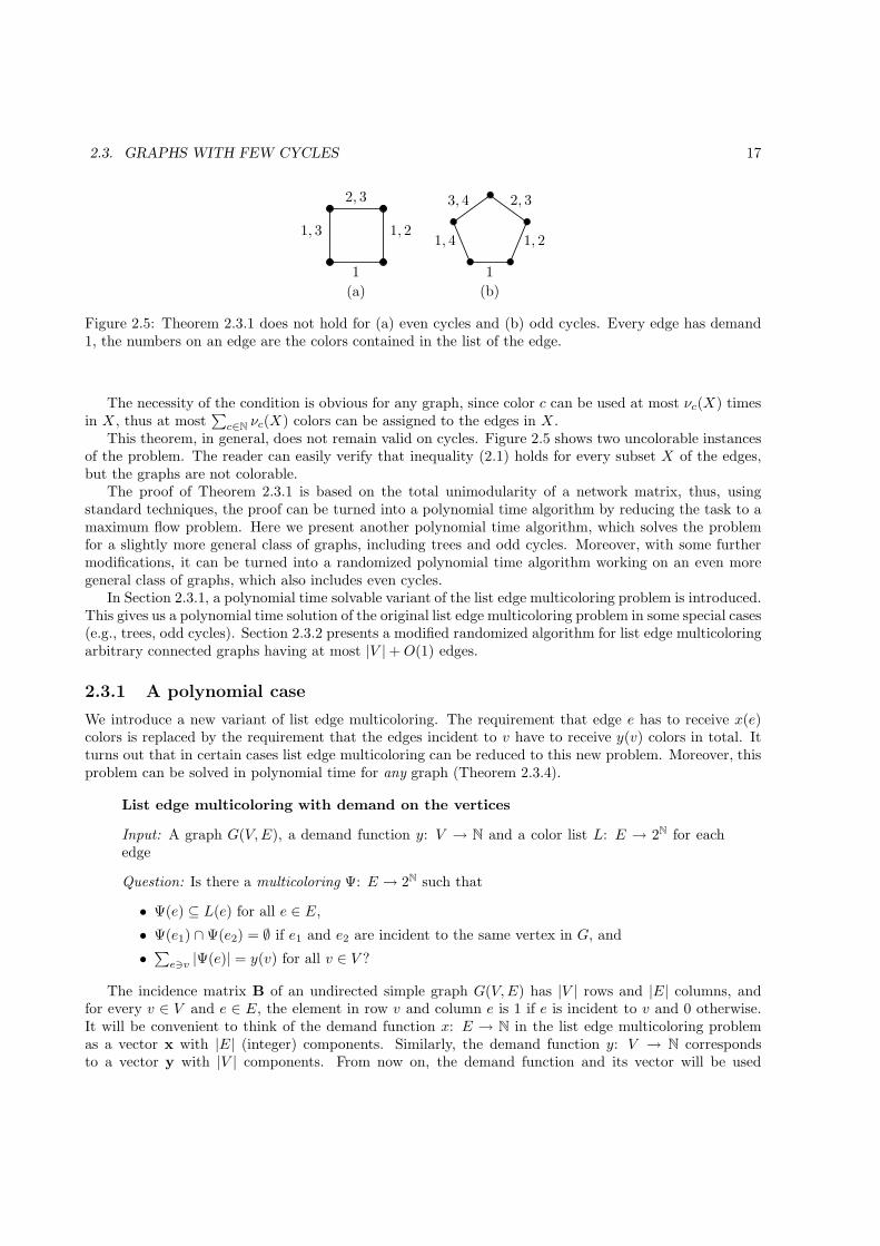
Figure 2.5: Theorem 2.3.1 does not hold for (a) even cycles and (b) odd cycles. Every edge has demand1, the numbers on an edge are the colors contained in the list of the edge.
The necessity of the condition is obvious for any graph, since color c can be used at most νc(X) timesin X , thus at most
∑c∈N
νc(X) colors can be assigned to the edges in X .This theorem, in general, does not remain valid on cycles. Figure 2.5 shows two uncolorable instances
of the problem. The reader can easily verify that inequality (2.1) holds for every subset X of the edges,but the graphs are not colorable.
The proof of Theorem 2.3.1 is based on the total unimodularity of a network matrix, thus, usingstandard techniques, the proof can be turned into a polynomial time algorithm by reducing the task to amaximum flow problem. Here we present another polynomial time algorithm, which solves the problemfor a slightly more general class of graphs, including trees and odd cycles. Moreover, with some furthermodifications, it can be turned into a randomized polynomial time algorithm working on an even moregeneral class of graphs, which also includes even cycles.
In Section 2.3.1, a polynomial time solvable variant of the list edge multicoloring problem is introduced.This gives us a polynomial time solution of the original list edge multicoloring problem in some special cases(e.g., trees, odd cycles). Section 2.3.2 presents a modified randomized algorithm for list edge multicoloringarbitrary connected graphs having at most |V | +O(1) edges.
2.3.1 A polynomial case
We introduce a new variant of list edge multicoloring. The requirement that edge e has to receive x(e)colors is replaced by the requirement that the edges incident to v have to receive y(v) colors in total. Itturns out that in certain cases list edge multicoloring can be reduced to this new problem. Moreover, thisproblem can be solved in polynomial time for any graph (Theorem 2.3.4).
List edge multicoloring with demand on the vertices
Input: A graph G(V,E), a demand function y: V → N and a color list L: E → 2N for eachedge
Question: Is there a multicoloring Ψ: E → 2N such that
• Ψ(e) ⊆ L(e) for all e ∈ E,
• Ψ(e1) ∩ Ψ(e2) = ∅ if e1 and e2 are incident to the same vertex in G, and
•∑
e∋v |Ψ(e)| = y(v) for all v ∈ V ?
The incidence matrix B of an undirected simple graph G(V,E) has |V | rows and |E| columns, andfor every v ∈ V and e ∈ E, the element in row v and column e is 1 if e is incident to v and 0 otherwise.It will be convenient to think of the demand function x: E → N in the list edge multicoloring problemas a vector x with |E| (integer) components. Similarly, the demand function y: V → N correspondsto a vector y with |V | components. From now on, the demand function and its vector will be used
18 CHAPTER 2. LIST COLORING
1, 2, 3
4
4
1, 2, 3
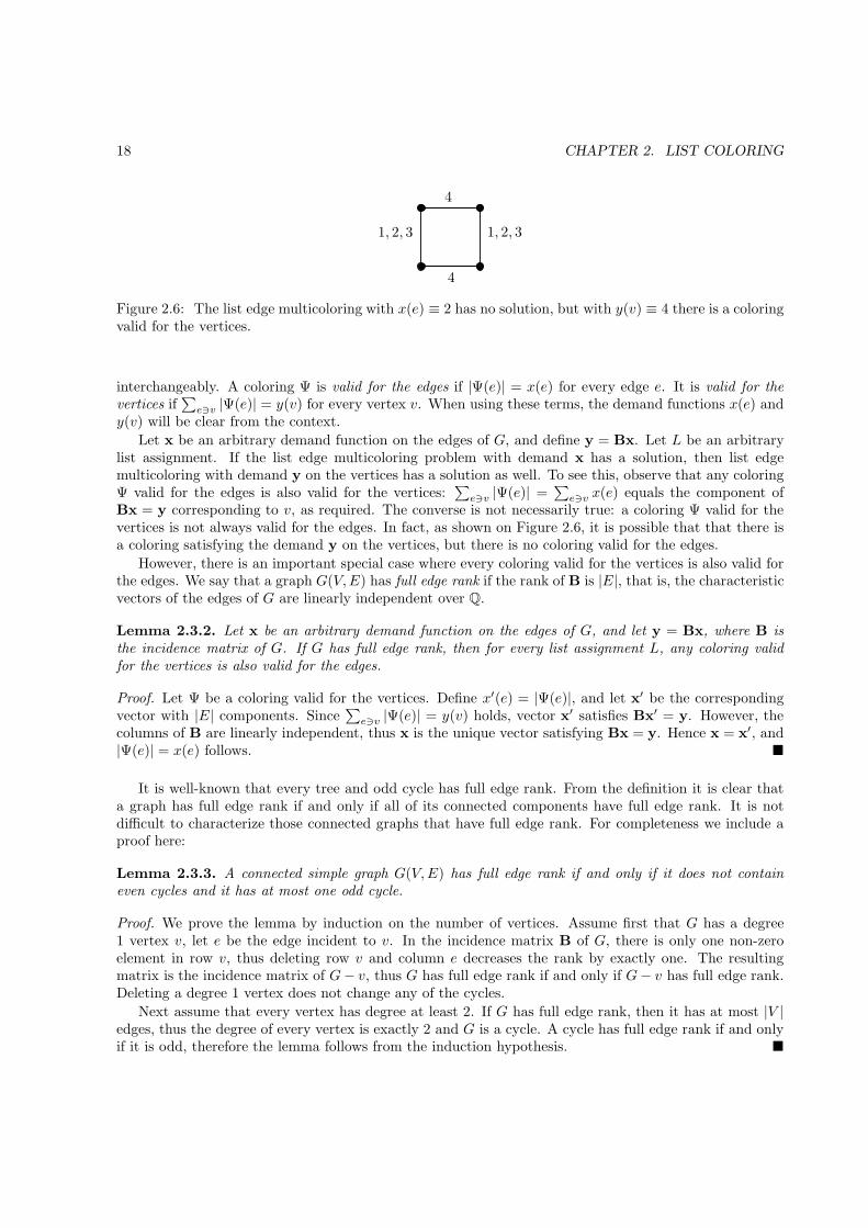
Figure 2.6: The list edge multicoloring with x(e) ≡ 2 has no solution, but with y(v) ≡ 4 there is a coloringvalid for the vertices.
interchangeably. A coloring Ψ is valid for the edges if |Ψ(e)| = x(e) for every edge e. It is valid for thevertices if
∑e∋v |Ψ(e)| = y(v) for every vertex v. When using these terms, the demand functions x(e) and
y(v) will be clear from the context.
Let x be an arbitrary demand function on the edges of G, and define y = Bx. Let L be an arbitrarylist assignment. If the list edge multicoloring problem with demand x has a solution, then list edgemulticoloring with demand y on the vertices has a solution as well. To see this, observe that any coloringΨ valid for the edges is also valid for the vertices:
∑e∋v |Ψ(e)| =
∑e∋v x(e) equals the component of
Bx = y corresponding to v, as required. The converse is not necessarily true: a coloring Ψ valid for thevertices is not always valid for the edges. In fact, as shown on Figure 2.6, it is possible that that there isa coloring satisfying the demand y on the vertices, but there is no coloring valid for the edges.
However, there is an important special case where every coloring valid for the vertices is also valid forthe edges. We say that a graph G(V,E) has full edge rank if the rank of B is |E|, that is, the characteristicvectors of the edges of G are linearly independent over Q.
Lemma 2.3.2. Let x be an arbitrary demand function on the edges of G, and let y = Bx, where B isthe incidence matrix of G. If G has full edge rank, then for every list assignment L, any coloring validfor the vertices is also valid for the edges.
Proof. Let Ψ be a coloring valid for the vertices. Define x′(e) = |Ψ(e)|, and let x′ be the correspondingvector with |E| components. Since
∑e∋v |Ψ(e)| = y(v) holds, vector x′ satisfies Bx′ = y. However, the
columns of B are linearly independent, thus x is the unique vector satisfying Bx = y. Hence x = x′, and|Ψ(e)| = x(e) follows. �
It is well-known that every tree and odd cycle has full edge rank. From the definition it is clear thata graph has full edge rank if and only if all of its connected components have full edge rank. It is notdifficult to characterize those connected graphs that have full edge rank. For completeness we include aproof here:
Lemma 2.3.3. A connected simple graph G(V,E) has full edge rank if and only if it does not containeven cycles and it has at most one odd cycle.
Proof. We prove the lemma by induction on the number of vertices. Assume first that G has a degree1 vertex v, let e be the edge incident to v. In the incidence matrix B of G, there is only one non-zeroelement in row v, thus deleting row v and column e decreases the rank by exactly one. The resultingmatrix is the incidence matrix of G− v, thus G has full edge rank if and only if G− v has full edge rank.Deleting a degree 1 vertex does not change any of the cycles.
Next assume that every vertex has degree at least 2. If G has full edge rank, then it has at most |V |edges, thus the degree of every vertex is exactly 2 and G is a cycle. A cycle has full edge rank if and onlyif it is odd, therefore the lemma follows from the induction hypothesis. �
2.3. GRAPHS WITH FEW CYCLES 19
We show that list edge multicoloring with demand on the vertices can be solved in polynomial time.Together with Lemma 2.3.2, this implies that the list edge multicoloring problem also can be solved inpolynomial time if the graph has full edge rank.
Theorem 2.3.4. For every simple graph G, list edge multicoloring with demand on the vertices can besolved in polynomial time.
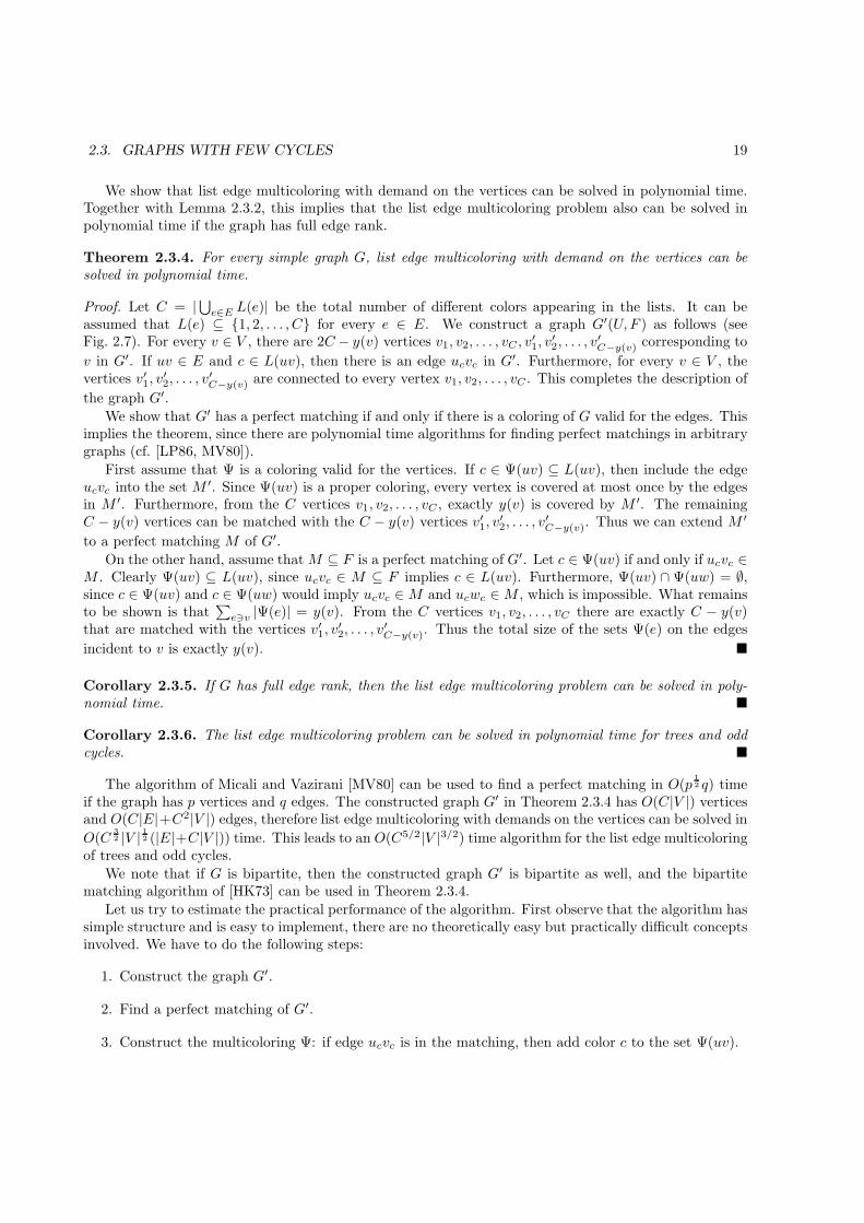
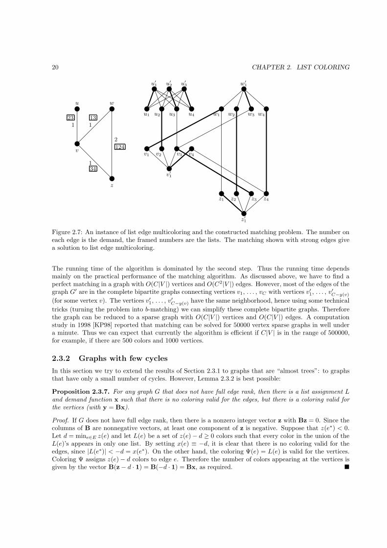
Proof. Let C = |⋃e∈E L(e)| be the total number of different colors appearing in the lists. It can be
assumed that L(e) ⊆ {1, 2, . . . , C} for every e ∈ E. We construct a graph G′(U,F ) as follows (seeFig. 2.7). For every v ∈ V , there are 2C − y(v) vertices v1, v2, . . . , vC , v
′1, v
′2, . . . , v
′C−y(v) corresponding to
v in G′. If uv ∈ E and c ∈ L(uv), then there is an edge ucvc in G′. Furthermore, for every v ∈ V , thevertices v′1, v
′2, . . . , v
′C−y(v) are connected to every vertex v1, v2, . . . , vC . This completes the description of
the graph G′.
We show that G′ has a perfect matching if and only if there is a coloring of G valid for the edges. Thisimplies the theorem, since there are polynomial time algorithms for finding perfect matchings in arbitrarygraphs (cf. [LP86, MV80]).
First assume that Ψ is a coloring valid for the vertices. If c ∈ Ψ(uv) ⊆ L(uv), then include the edgeucvc into the set M ′. Since Ψ(uv) is a proper coloring, every vertex is covered at most once by the edgesin M ′. Furthermore, from the C vertices v1, v2, . . . , vC , exactly y(v) is covered by M ′. The remainingC − y(v) vertices can be matched with the C − y(v) vertices v′1, v
′2, . . . , v
′C−y(v). Thus we can extend M ′
to a perfect matching M of G′.
On the other hand, assume that M ⊆ F is a perfect matching of G′. Let c ∈ Ψ(uv) if and only if ucvc ∈M . Clearly Ψ(uv) ⊆ L(uv), since ucvc ∈ M ⊆ F implies c ∈ L(uv). Furthermore, Ψ(uv) ∩ Ψ(uw) = ∅,since c ∈ Ψ(uv) and c ∈ Ψ(uw) would imply ucvc ∈M and ucwc ∈M , which is impossible. What remainsto be shown is that
∑e∋v |Ψ(e)| = y(v). From the C vertices v1, v2, . . . , vC there are exactly C − y(v)
that are matched with the vertices v′1, v′2, . . . , v
′C−y(v). Thus the total size of the sets Ψ(e) on the edges
incident to v is exactly y(v). �
Corollary 2.3.5. If G has full edge rank, then the list edge multicoloring problem can be solved in poly-nomial time. �
Corollary 2.3.6. The list edge multicoloring problem can be solved in polynomial time for trees and oddcycles. �
The algorithm of Micali and Vazirani [MV80] can be used to find a perfect matching in O(p12 q) time
if the graph has p vertices and q edges. The constructed graph G′ in Theorem 2.3.4 has O(C|V |) verticesand O(C|E|+C2|V |) edges, therefore list edge multicoloring with demands on the vertices can be solved in
O(C32 |V |
12 (|E|+C|V |)) time. This leads to an O(C5/2|V |3/2) time algorithm for the list edge multicoloring
of trees and odd cycles.
We note that if G is bipartite, then the constructed graph G′ is bipartite as well, and the bipartitematching algorithm of [HK73] can be used in Theorem 2.3.4.
Let us try to estimate the practical performance of the algorithm. First observe that the algorithm hassimple structure and is easy to implement, there are no theoretically easy but practically difficult conceptsinvolved. We have to do the following steps:
1. Construct the graph G′.
2. Find a perfect matching of G′.
3. Construct the multicoloring Ψ: if edge ucvc is in the matching, then add color c to the set Ψ(uv).
20 CHAPTER 2. LIST COLORING
w′
1
u3u2 u4u1
2
134
13
124
1123
u w
v
z
v1 v4v3v2
v′1
u′
1 u′
2 u′
3
z′1
z1 z2 z3 z4
w3 w4w1 w2
Figure 2.7: An instance of list edge multicoloring and the constructed matching problem. The number oneach edge is the demand, the framed numbers are the lists. The matching shown with strong edges givea solution to list edge multicoloring.
The running time of the algorithm is dominated by the second step. Thus the running time dependsmainly on the practical performance of the matching algorithm. As discussed above, we have to find aperfect matching in a graph with O(C|V |) vertices and O(C2|V |) edges. However, most of the edges of thegraph G′ are in the complete bipartite graphs connecting vertices v1, . . . , vC with vertices v′1, . . . , v′C−y(v)
(for some vertex v). The vertices v′1, . . . , v′C−y(v) have the same neighborhood, hence using some technical
tricks (turning the problem into b-matching) we can simplify these complete bipartite graphs. Thereforethe graph can be reduced to a sparse graph with O(C|V |) vertices and O(C|V |) edges. A computationstudy in 1998 [KP98] reported that matching can be solved for 50000 vertex sparse graphs in well undera minute. Thus we can expect that currently the algorithm is efficient if C|V | is in the range of 500000,for example, if there are 500 colors and 1000 vertices.
2.3.2 Graphs with few cycles
In this section we try to extend the results of Section 2.3.1 to graphs that are “almost trees”: to graphsthat have only a small number of cycles. However, Lemma 2.3.2 is best possible:
Proposition 2.3.7. For any graph G that does not have full edge rank, then there is a list assignment Land demand function x such that there is no coloring valid for the edges, but there is a coloring valid forthe vertices (with y = Bx).
Proof. If G does not have full edge rank, then there is a nonzero integer vector z with Bz = 0. Since thecolumns of B are nonnegative vectors, at least one component of z is negative. Suppose that z(e∗) < 0.Let d = mine∈E z(e) and let L(e) be a set of z(e) − d ≥ 0 colors such that every color in the union of theL(e)’s appears in only one list. By setting x(e) ≡ −d, it is clear that there is no coloring valid for theedges, since |L(e∗)| < −d = x(e∗). On the other hand, the coloring Ψ(e) = L(e) is valid for the vertices.Coloring Ψ assigns z(e) − d colors to edge e. Therefore the number of colors appearing at the vertices isgiven by the vector B(z − d · 1) = B(−d · 1) = Bx, as required. �
2.3. GRAPHS WITH FEW CYCLES 21
On the other hand, we show that if a coloring Ψ is valid for the vertices and it satisfies some additionalconstraints, then it is also valid for the edges.
Lemma 2.3.8. Let G(V,E) be an arbitrary graph, and let E′ ⊆ E be a subset of edges such that the graphG′(V,E \E′) has full edge rank. For an arbitrary demand function x and list assignment L, if coloring Ψis valid for the vertices and it satisfies |Ψ(e)| = x(e) for every e ∈ E′, then Ψ is also valid for the edges.
Proof. It can be assumed that the edges in E′ correspond to the first |E′| columns of B. Therefore B canbe written as B = (B1 B2), where B1 has |E′| columns. Similarly x =
(x1
x2
)and x1 has |E′| components.
Clearly, y = Bx = B1x1 + B2x2.
Let x′(e) = |Ψ(e)| and let x′ =(x′
1
x′
2
)be the corresponding vector. Since Ψ is valid for the vertices, it
follows that Bx′ = Bx = y, that is
B1x′1 + B2x
′2 = B1x1 + B2x2 = y.
Moreover, since |Ψ(e)| = x(e) for every e ∈ E′, we have that x′1 = x1, B1x
′1 = B1x1, and B2x
′2 = B2x2
follows. Since G′(V,E \ E′) has full edge rank, the columns of the matrix B2 are linearly independent,hence x′
2 = x2. Therefore x′ = x, and Ψ is valid for the edges. �
Since every coloring that is valid for the edges is also valid for the vertices, the list edge multicoloringproblem has a solution if and only if there is a coloring valid for the vertices that satisfies the requirementsin Lemma 2.3.8. We reduce the problem of finding such a coloring to a variant of the exact matchingproblem, which can be solved in randomized polynomial time. Before presenting the reduction (whichis essentially the same as in the proof of Theorem 2.3.4), we briefly overview exact matching and somerelated problems.
There are strongly polynomial time algorithms for finding a maximum weight perfect matching ina graph (cf. [LP86]). That is, it can be decided in polynomial time whether a perfect matching withweight at least K exists. In the exact matching problem we have to find a perfect matching whose weightequals K. The exact matching problem can be solved in randomized polynomial time if every weight isan integer smaller than some polynomial of the size of the graph [MVV87]. That is, there is a polynomialtime algorithm that answers “no” if there is no matching with weight exactly K, and answers “yes” withprobability at least 1
2 if there is such a matching. It is an open question whether there exists a deterministicpolynomial time algorithm for this problem.
A related problem is the following: given a graph G(V,E), a set of edges F ⊆ E, and an integer k,find a perfect matching M of G with |M ∩ F | = k. This can be reduced to the exact matching problem:let every edge in F have weight 1 and every other edge weight 0. Now a matching M has |M ∩ F | = k ifand only if its weight equals k. More generally, we can consider more than one subset of the edges:
Proposition 2.3.9. Assume that we are given a graph G(V,E), pairwise disjoint subsets F0, F1, . . . , Fℓ ⊆E, and integers k0, k1, . . . , kℓ. If ℓ is fixed, then it can be decided in randomized polynomial time whetherthere is a perfect matching M with |M ∩ Fi| = ki for every 0 ≤ i ≤ ℓ.
Proof. This problem can be reduced to exact matching: let e ∈ Fi have weight (|E| + 1)i, edges in
E \ (F0 ∪ · · · ∪Fℓ) have weight 0, and set K =∑ℓ
i=0 ki(|E|+ 1)i. It is easy to see that a matching satisfiesthe requirements if and only if it has weight K. If ℓ is a fixed constant, then the weight of every edge ispolynomially bounded in the size of the graph, thus the problem can be solved in randomized polynomialtime. �
Theorem 2.3.10. For every fixed ℓ, there is a randomized polynomial time algorithm for list edge multi-coloring in connected graphs having at most |V | + ℓ edges.
22 CHAPTER 2. LIST COLORING
Proof. Let T be a spanning tree of G(V,E), and let E′ = {e0, e1, . . . , eℓ} be the |E| − (|V | − 1) = ℓ + 1edges not in T . Notice that E \E′ has full edge rank (it is a tree). Construct the graph G′, as in the proofof Theorem 2.3.4. For every 0 ≤ i ≤ ℓ, let Fi contain the |L(ei)| edges in G′ that corresponds to edge ei.That is, if ei = uv and L(ei) = {c1, c2, . . . , cr}, then Fi = {uc1vc1 , uc2vc2 , . . . , ucr
vcr}. Set ki to x(ei).
We show that the list edge multicoloring problem has a solution if and only if G′ has a perfect matchingM with |Fi ∩M | = ki for every 0 ≤ i ≤ ℓ. By Prop. 2.3.9, the latter problem can be solved in randomizedpolynomial time, hence the theorem follows.
If there is a perfect matching M in G such that |Fi ∩M | = ki for every 0 ≤ i ≤ ℓ, then construct acoloring Ψ valid for the vertices, as in the proof of Theorem 2.3.4. Clearly, |Ψ(ei)| = ki = x(ei). Thus byLemma 2.3.8, Ψ is valid for the edges.
The other direction also follows easily: since any coloring Ψ valid for the edges is also valid for thevertices, one can find a perfect matching M of G′ based on Ψ. It is clear from the construction that Mhas exactly ki edges from Fi, since |Ψ(ei)| = x(ei) = ki. �
Corollary 2.3.11. List edge multicoloring can be solved in randomized polynomial time for even cycles.�
2.3.3 Applications and extensions
List edge multicoloring can be applied to model the scheduling of file transfers between processors. Letthe vertices be the processors, if there is an edge e with demand x(e) between two vertices, then thismeans that there is a direct connection between the two processors and a file has to be transfered on thisconnection. The file transfer represented by the edge e requires x(e) time slots. The colors correspond tothe time slots, thus by assigning color sets to the edges we can schedule the file transfers. The requirementthat every color appears at most once at a vertex ensures that a processor performs at most one transferat the same time. Furthermore, by setting the lists of the edges appropriately, we can express additionalconstraints. For example, we can require that a transfer is not started before a certain time, or it isfinished before a certain deadline. Corollary 2.3.6 and Theorem 2.3.10 give efficient algorithms for thisproblem if the topology of the network is almost a tree. The same method can be applied to model themutual diagnostic testing of processors: in this case an edge e with demand x(e) means that the twoprocessors have to test each other for x(e) units of time.
In the application examples of the previous paragraph we have assumed that a processor can do onlyone thing at the same time. This requirement can be weakened: we can consider the variant of the problemwhere a processor can participate in at most f file transfers simultaneously. More generally, this numberf can be different for the different processors. This leads to the f -coloring problem [ZN99, ZFN00]: givena function f on the vertices, we have to find a coloring where every color appears at most f(v) times atvertex v. This more general problem can be handled with a similar reduction to matching. However, nowwe have to allow that at most f(v) edges incident to a vertex vc are selected into the matching. Thusthe problem can be formulated as a b-matching, we omit the straightforward details. (The b-matchingproblem is a generalization of matching: we have a function b on the vertices, and the task is to find a setof edges such that exactly b(v) edges are incident to vertex v.)
List edge multicoloring turns out to be useful in a different scheduling model as well. Let us assumethat there are n days and m workers. On the ith day x(i) workers are required. The jth worker isavailable only on days W (i) ⊆ {1, . . . , n} and it is not allowed to use a worker on two consecutive days.This problem can be formulated as list edge multicoloring on a path: the edges e1, e2, . . . , en of the pathcorrespond to the days, the colors correspond to the workers. The demand of edge ei is x(i) and its list is{j : i ∈W (j)}, the set of workers available on the ith day. A list edge multicoloring of the path is clearlyequivalent to an allowed job assignment. List multicoloring of paths, which is the same problem as thelist edge multicoloring of paths, was investigated [KG02].
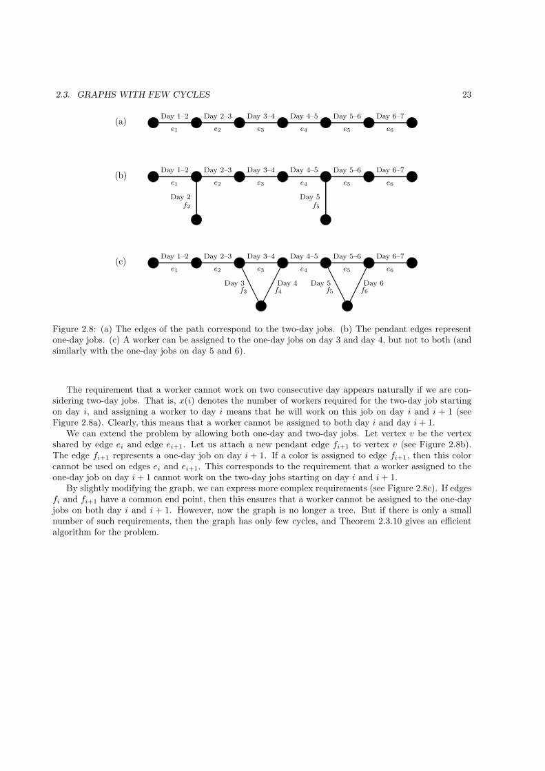
2.3. GRAPHS WITH FEW CYCLES 23
e2
e2
e2
e3
e3
e3
e4
e4
e4
e5
e5
e5
e6
e6
e6
(a)
f2
f6f5
f5
f4f3
(b)
Day 2
Day 1–2
Day 1–2
Day 1–2
Day 2–3
Day 2–3
Day 2–3
Day 3–4
Day 3–4
Day 3–4
Day 4–5
Day 4–5
Day 4–5
Day 5–6
Day 5–6
Day 5–6
Day 6–7
Day 6–7
Day 6–7
Day 4Day 3 Day 5
Day 5
Day 6
(c)e1
e1
e1
Figure 2.8: (a) The edges of the path correspond to the two-day jobs. (b) The pendant edges representone-day jobs. (c) A worker can be assigned to the one-day jobs on day 3 and day 4, but not to both (andsimilarly with the one-day jobs on day 5 and 6).
The requirement that a worker cannot work on two consecutive day appears naturally if we are con-sidering two-day jobs. That is, x(i) denotes the number of workers required for the two-day job startingon day i, and assigning a worker to day i means that he will work on this job on day i and i + 1 (seeFigure 2.8a). Clearly, this means that a worker cannot be assigned to both day i and day i+ 1.
We can extend the problem by allowing both one-day and two-day jobs. Let vertex v be the vertexshared by edge ei and edge ei+1. Let us attach a new pendant edge fi+1 to vertex v (see Figure 2.8b).The edge fi+1 represents a one-day job on day i + 1. If a color is assigned to edge fi+1, then this colorcannot be used on edges ei and ei+1. This corresponds to the requirement that a worker assigned to theone-day job on day i+ 1 cannot work on the two-day jobs starting on day i and i+ 1.
By slightly modifying the graph, we can express more complex requirements (see Figure 2.8c). If edgesfi and fi+1 have a common end point, then this ensures that a worker cannot be assigned to the one-dayjobs on both day i and i + 1. However, now the graph is no longer a tree. But if there is only a smallnumber of such requirements, then the graph has only few cycles, and Theorem 2.3.10 gives an efficientalgorithm for the problem.

CHAPTER 3
Precoloring extension
To finish a work? To finish a picture? What nonsense! To finish itmeans to be through with it, to kill it, to rid it of its soul,
to give it its final blow . . . the coup de gracefor the painter as well as for the picture.
Pablo Picasso (1881–1973)
In the precoloring extension problem we are given a graph G(V,E) with a subset W of precoloredvertices, and it has to be decided whether this coloring can be extended to the whole graph. The problemis formally defined as follows:
Precoloring Extension (PrExt)
Input: A graph G(V,E), a subset W ⊆ V , a coloring ψ′ of W and an integer k.
Question: Is there a proper k-coloring ψ of G extending the coloring ψ′ (that is, ψ(v) = ψ′(v)for every v ∈ W )?
The special case of the problem where every color is used at most d times in the precoloring will bedenoted by d-PrExt. In particular, we will focus on the 1-PrExt problem.
Since vertex coloring is a special case of precoloring extension with W = ∅, thus PrExt is NP-complete for every class of graphs where vertex coloring is NP-complete. Therefore we can hope to solvePrExt efficiently only on graphs that are easy to color. In the 90s, Biro, Hujter and Tuza [BHT92,HT93, HT96] started a systematic study of precoloring extension in perfect graphs, where coloring canbe done in polynomial time. It turns out that for some classes of perfect graphs, e.g., split graphs[HT93], complements of bipartite graphs [HT93], and cographs [HT96, JS97], the precoloring extensionproblem can be solved in polynomial time. On the other hand, for some other classes like bipartitegraphs [HT93, BJW94], line graphs of bipartite graphs [EP01, Col84, Fia03], and interval graphs [BHT92],precoloring extension is NP-complete.
Precoloring extension can be also thought of as a special case of list coloring. The list of a precoloredvertex contains only a single color, while if a vertex is not precolored, then its list contains all the availablecolors. Therefore any hardness result obtained for precoloring extension applies also for list coloring.
26 CHAPTER 3. PRECOLORING EXTENSION
Motivated by the aircraft scheduling application presented in Chapter 1, Biro, Hujter, and Tuza studiedthe precoloring extension problem for interval graphs [BHT92, BHT93]. They have shown that PrExt
(in fact, even 2-PrExt) is NP-complete for interval graphs, but 1-PrExt is polynomial-time solvable. In[HT96] they formulate two open questions concerning the possible strengthening of these results:
• Is it possible to solve 1-PrExt in polynomial time for chordal graphs? (A graph is chordal if it doesnot contain induced cycles of length greater than 3. Every interval graph is chordal.)
• Does PrExt remain NP-complete restricted to unit interval graphs? (A unit interval graph is aninterval graph that can be represented by unit length intervals.)
We give positive answers to both questions. In Section 3.1 a polynomial-time algorithm is presented for1-PrExt on chordal graphs, a class generalizing interval graphs. In Section 3.3 we show that PrExt
is NP-complete not only for interval graphs, but even for the smaller class of unit interval graphs. Theproof is by reduction from a disjoint paths problem. The NP-completeness of this disjoint paths problemis proved in Section 3.2. The result on the disjoint paths problem is of independent interest: it answersan open question of Vygen [Vyg94].
Finally, Section 3.4 gives complexity results on the edge coloring version of precoloring extension.Easton and Parker [EP01], and independently Fiala [Fia03] have shown that the problem is NP-completefor bipartite graphs of maximum degree 3. In Section 3.4 we strengthen this result by showing that theproblem remains NP-complete for planar 3-regular bipartite graphs. This result will be used in Section 5.2to prove that minimum sum edge coloring is NP-hard for planar bipartite graphs. Section 3.4 also showsthat precoloring edge extension is NP-complete for outerplanar and series-parallel graphs. The reductionsare from the corresponding list edge coloring problems investigated in Section 2.1.1.
The results in Section 3.1 were presented in [Mar04j]. The results of Section 3.2 appeared in [Mar04d].The results of Section 3.3 and Section 3.4 will appear in [Mar04k] and [Mar04i], respectively.
3.1 Chordal graphs
The aim of this section is to prove that 1-PrExt is polynomial-time solvable for chordal graphs, whichanswers an open question of Hujter and Tuza [HT96]. It is easy to reduce PrExt to 1-PrExt: collapsethe vertices precolored with the same color to a single vertex. Therefore 1-PrExt is not easier thanPrExt on classes of graphs that are closed for this operation. One can also show that 1-PrExt isNP-complete on bipartite graphs [HT93, BJW94].
However, there are cases where 1-PrExt is strictly easier than PrExt. For planar bipartite graphs,if the set of colors C contains only 3 colors, then PrExt is NP-complete [Kra93], while 1-PrExt can besolved in polynomial time [MTW98]. For interval graphs already 2-PrExt is NP-complete [BHT92], but1-PrExt can be solved in polynomial time [BHT92].
Every chordal graph is perfect and interval graphs form a subset of chordal graphs (cf. [Gol80]).Therefore from the NP-completeness of 2-PrExt for interval graphs [BHT92] it follows that the problemis NP-complete for chordal graphs as well. The complexity of 1-PrExt on chordal graphs is posed byHujter and Tuza as an open question [HT96]. Here we show that 1-PrExt can be solved in polynomialtime also for chordal graphs. The algorithm is a generalization of the method of [BHT92] for intervalgraphs. As in [BHT92], 1-PrExt is reduced to a network flow problem, but for chordal graphs a moreelaborate construction is required than for interval graphs.
In Section 3.1.1 we review some known properties of chordal graphs. In Section 3.1.2 we define a setsystem that will be crucial in the analysis of the algorithm. The algorithm is presented in Section 3.1.3.In Section 3.1.4 we discuss some connections of the problem with matroid theory.
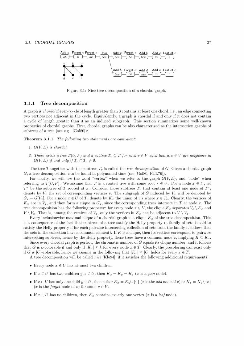
3.1. CHORDAL GRAPHS 27
cdv
ab bvJoinAdd a Forget v Forget c
bc
av
d
b
b
Leaf of c
e
e
Leaf of eAdd v
Add v
Forget e Add b
Add b
Add ccebce
cc
cv cv
bcv
bcv
bcv
Forget d Add d
Figure 3.1: Nice tree decomposition of a chordal graph.
3.1.1 Tree decomposition
A graph is chordal if every cycle of length greater than 3 contains at least one chord, i.e., an edge connectingtwo vertices not adjacent in the cycle. Equivalently, a graph is chordal if and only if it does not containa cycle of length greater than 3 as an induced subgraph. This section summarizes some well-knownproperties of chordal graphs. First, chordal graphs can be also characterized as the intersection graphs ofsubtrees of a tree (see e.g., [Gol80]):
Theorem 3.1.1. The following two statements are equivalent:
1. G(V,E) is chordal.
2. There exists a tree T (U,F ) and a subtree Tv ⊆ T for each v ∈ V such that u, v ∈ V are neighbors inG(V,E) if and only if Tu ∩ Tv 6= ∅.
The tree T together with the subtrees Tv is called the tree decomposition of G. Given a chordal graphG, a tree decomposition can be found in polynomial time (see [Gol80, RTL76]).
For clarity, we will use the word “vertex” when we refer to the graph G(V,E), and “node” whenreferring to T (U,F ). We assume that T is a rooted tree with some root r ∈ U . For a node x ∈ U , letT x be the subtree of T rooted at x. Consider those subtrees Tv that contain at least one node of T x,denote by Vx the set of corresponding vertices v. The subgraph of G induced by Vx will be denoted byGx = G[Vx]. For a node x ∈ U of T , denote by Kx the union of v’s where x ∈ Tv. Clearly, the vertices ofKx are in Vx, and they form a clique in Gx, since the corresponding trees intersect in T at node x. Thetree decomposition has the following property: for every node x ∈ U , the clique Kx separates Vx \Kx andV \ Vx. That is, among the vertices of Vx, only the vertices in Kx can be adjacent to V \ Vx.
Every inclusionwise maximal clique of a chordal graph is a clique Kx of the tree decomposition. Thisis a consequence of the fact that subtrees of a tree satisfy the Helly property (a family of sets is said tosatisfy the Helly property if for each pairwise intersecting collection of sets from the family it follows thatthe sets in the collection have a common element). If K is a clique, then its vertices correspond to pairwiseintersecting subtrees, hence by the Helly property, these trees have a common node x, implying K ⊆ Kx.
Since every chordal graph is perfect, the chromatic number of G equals its clique number, and it followsthat G is k-colorable if and only if |Kx| ≤ k for every node x ∈ T . Clearly, the precoloring can exist onlyif G is |C|-colorable, hence we assume in the following that |Kx| ≤ |C| holds for every x ∈ T .
A tree decomposition will be called nice [Klo94], if it satisfies the following additional requirements:
• Every node x ∈ U has at most two children.
• If x ∈ U has two children y, z ∈ U , then Kx = Ky = Kz (x is a join node).
• If x ∈ U has only one child y ∈ U , then either Kx = Ky∪{v} (x is the add node of v) or Kx = Ky\{v}(x is the forget node of v) for some v ∈ V .
• If x ∈ U has no children, then Kx contains exactly one vertex (x is a leaf node).
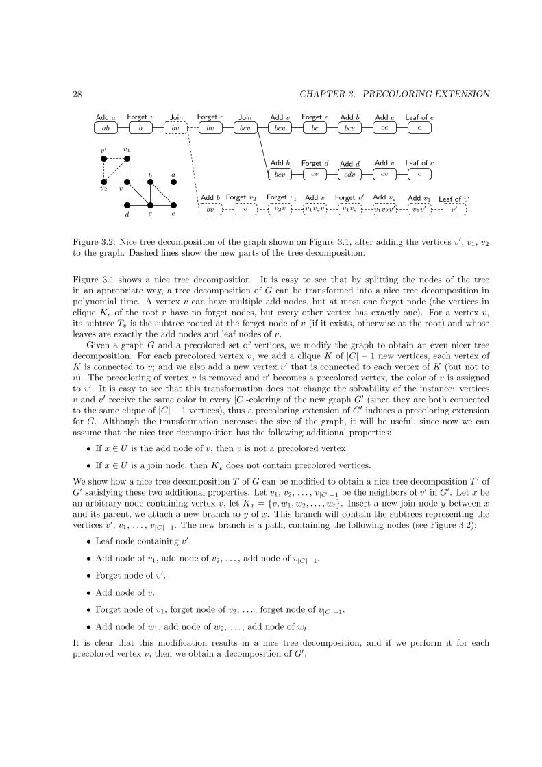
28 CHAPTER 3. PRECOLORING EXTENSION
a
bc
Leaf of eForget e Add c
cebce
Forget vAdd a
ab
Forget c JoinJoin
v1v2vvbv
bvbv
v1v2 v1v2v′ v1v′Leaf of v′Add v1Add v2Forget v′Forget v1
v2v
Forget v2
bcv
bcv bcv
cvcv
Leaf of cAdd v
Add v
Add v
Add b
Add b
Add b
Forget d Add d
cdv
v2
v′
v′
v1
v
b
b
c
c
e
e
d
Figure 3.2: Nice tree decomposition of the graph shown on Figure 3.1, after adding the vertices v′, v1, v2to the graph. Dashed lines show the new parts of the tree decomposition.
Figure 3.1 shows a nice tree decomposition. It is easy to see that by splitting the nodes of the treein an appropriate way, a tree decomposition of G can be transformed into a nice tree decomposition inpolynomial time. A vertex v can have multiple add nodes, but at most one forget node (the vertices inclique Kr of the root r have no forget nodes, but every other vertex has exactly one). For a vertex v,its subtree Tv is the subtree rooted at the forget node of v (if it exists, otherwise at the root) and whoseleaves are exactly the add nodes and leaf nodes of v.
Given a graph G and a precolored set of vertices, we modify the graph to obtain an even nicer treedecomposition. For each precolored vertex v, we add a clique K of |C| − 1 new vertices, each vertex ofK is connected to v; and we also add a new vertex v′ that is connected to each vertex of K (but not tov). The precoloring of vertex v is removed and v′ becomes a precolored vertex, the color of v is assignedto v′. It is easy to see that this transformation does not change the solvability of the instance: verticesv and v′ receive the same color in every |C|-coloring of the new graph G′ (since they are both connectedto the same clique of |C| − 1 vertices), thus a precoloring extension of G′ induces a precoloring extensionfor G. Although the transformation increases the size of the graph, it will be useful, since now we canassume that the nice tree decomposition has the following additional properties:
• If x ∈ U is the add node of v, then v is not a precolored vertex.
• If x ∈ U is a join node, then Kx does not contain precolored vertices.
We show how a nice tree decomposition T of G can be modified to obtain a nice tree decomposition T ′ ofG′ satisfying these two additional properties. Let v1, v2, . . . , v|C|−1 be the neighbors of v′ in G′. Let x bean arbitrary node containing vertex v, let Kx = {v, w1, w2, . . . , wt}. Insert a new join node y between xand its parent, we attach a new branch to y of x. This branch will contain the subtrees representing thevertices v′, v1, . . . , v|C|−1. The new branch is a path, containing the following nodes (see Figure 3.2):
• Leaf node containing v′.
• Add node of v1, add node of v2, . . . , add node of v|C|−1.
• Forget node of v′.
• Add node of v.
• Forget node of v1, forget node of v2, . . . , forget node of v|C|−1.
• Add node of w1, add node of w2, . . . , add node of wt.
It is clear that this modification results in a nice tree decomposition, and if we perform it for eachprecolored vertex v, then we obtain a decomposition of G′.
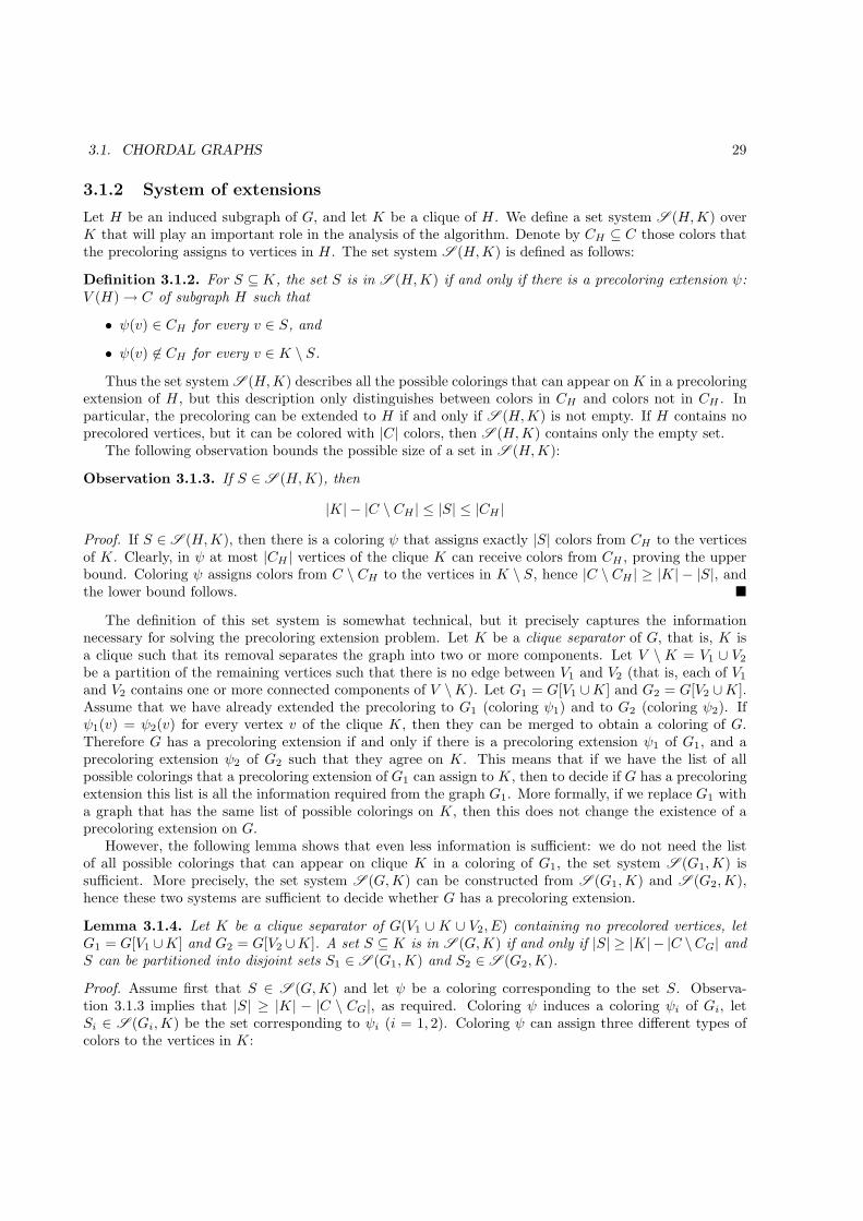
3.1. CHORDAL GRAPHS 29
3.1.2 System of extensions
Let H be an induced subgraph of G, and let K be a clique of H . We define a set system S (H,K) overK that will play an important role in the analysis of the algorithm. Denote by CH ⊆ C those colors thatthe precoloring assigns to vertices in H . The set system S (H,K) is defined as follows:
Definition 3.1.2. For S ⊆ K, the set S is in S (H,K) if and only if there is a precoloring extension ψ:V (H) → C of subgraph H such that
• ψ(v) ∈ CH for every v ∈ S, and
• ψ(v) 6∈ CH for every v ∈ K \ S.
Thus the set system S (H,K) describes all the possible colorings that can appear on K in a precoloringextension of H , but this description only distinguishes between colors in CH and colors not in CH . Inparticular, the precoloring can be extended to H if and only if S (H,K) is not empty. If H contains noprecolored vertices, but it can be colored with |C| colors, then S (H,K) contains only the empty set.
The following observation bounds the possible size of a set in S (H,K):
Observation 3.1.3. If S ∈ S (H,K), then
|K| − |C \ CH | ≤ |S| ≤ |CH |
Proof. If S ∈ S (H,K), then there is a coloring ψ that assigns exactly |S| colors from CH to the verticesof K. Clearly, in ψ at most |CH | vertices of the clique K can receive colors from CH , proving the upperbound. Coloring ψ assigns colors from C \ CH to the vertices in K \ S, hence |C \ CH | ≥ |K| − |S|, andthe lower bound follows. �
The definition of this set system is somewhat technical, but it precisely captures the informationnecessary for solving the precoloring extension problem. Let K be a clique separator of G, that is, K isa clique such that its removal separates the graph into two or more components. Let V \ K = V1 ∪ V2
be a partition of the remaining vertices such that there is no edge between V1 and V2 (that is, each of V1
and V2 contains one or more connected components of V \K). Let G1 = G[V1 ∪K] and G2 = G[V2 ∪K].Assume that we have already extended the precoloring to G1 (coloring ψ1) and to G2 (coloring ψ2). Ifψ1(v) = ψ2(v) for every vertex v of the clique K, then they can be merged to obtain a coloring of G.Therefore G has a precoloring extension if and only if there is a precoloring extension ψ1 of G1, and aprecoloring extension ψ2 of G2 such that they agree on K. This means that if we have the list of allpossible colorings that a precoloring extension of G1 can assign to K, then to decide if G has a precoloringextension this list is all the information required from the graph G1. More formally, if we replace G1 witha graph that has the same list of possible colorings on K, then this does not change the existence of aprecoloring extension on G.
However, the following lemma shows that even less information is sufficient: we do not need the listof all possible colorings that can appear on clique K in a coloring of G1, the set system S (G1,K) issufficient. More precisely, the set system S (G,K) can be constructed from S (G1,K) and S (G2,K),hence these two systems are sufficient to decide whether G has a precoloring extension.
Lemma 3.1.4. Let K be a clique separator of G(V1 ∪ K ∪ V2, E) containing no precolored vertices, letG1 = G[V1 ∪K] and G2 = G[V2 ∪K]. A set S ⊆ K is in S (G,K) if and only if |S| ≥ |K| − |C \CG| andS can be partitioned into disjoint sets S1 ∈ S (G1,K) and S2 ∈ S (G2,K).
Proof. Assume first that S ∈ S (G,K) and let ψ be a coloring corresponding to the set S. Observa-tion 3.1.3 implies that |S| ≥ |K| − |C \ CG|, as required. Coloring ψ induces a coloring ψi of Gi, letSi ∈ S (Gi,K) be the set corresponding to ψi (i = 1, 2). Coloring ψ can assign three different types ofcolors to the vertices in K:

30 CHAPTER 3. PRECOLORING EXTENSION
• If ψ(v) 6∈ CG (i.e., ψ(v) is not used in the precoloring), then v 6∈ S, S1, S2.
• If the precoloring uses ψ(v) in V1, then v ∈ (S ∩ S1) \ S2. (Since each color is used at most once inthe precoloring, ψ(v) cannot appear in V2 on a precolored vertex.)
• If the precoloring uses ψ(v) in V2, then v ∈ (S ∩ S2) \ S1.
Note that v cannot be a precolored vertex, hence the precoloring cannot use ψ(v) in K. Therefore S isthe disjoint union of S1 and S2, as required.
Now assume that S can be partitioned into disjoint sets S1 ∈ S (G1,K) and S2 ∈ S (G2,K), let ψ1
and ψ2 be the two corresponding colorings. In general, ψ1 and ψ2 might be different on K, thus theycannot be combined to obtain a coloring of G. However, with some permutations of colors we modifythe two colorings in such a way that they assign the same color to every vertex of K. Let C1 (resp. C2)be the colors of the precolored vertices in V1 (resp. V2). Notice that both ψ1 and ψ2 assign colors fromC \ C1 to S2, (since S1 and S2 are disjoint). Modify coloring ψ1: permute the colors of C \ C1 such thatψ1(v) = ψ2(v) holds for every v ∈ S2 (this can be done since K is a clique, hence both ψ1 and ψ2 assigndistinct colors to the vertices in S2). Since the precolored vertices in V1 have colors only from C1, coloringψ1 remains a valid precoloring extension for G1. Similarly, in coloring ψ2, permute the colors of C \ C2
such that ψ1(v) = ψ2(v) for every v ∈ S1. Now we have that ψ1 and ψ2 agree on S, there might bedifferences only on K \ S. Moreover, ψ1 uses only colors from C \ C1 on K \ S, and ψ2 uses colors onlyfrom C \C2 on this set. Now select a set C′ ⊆ C \CG such that |C′| = |K \S| (here we use the assumption|S| ≥ |K| − |C \ CG|, which implies that there are enough colors in C \ CG). Permute again the colorsof C \ C1 in coloring ψ1 such that ψ1 assigns to K \ S exactly the colors in C′. Similarly, permute thecolors of C \C2 in coloring ψ2 such that ψ2 also uses C′ on K \ S. Now the colorings ψ1 and ψ2 agree onK, hence we can combine them to obtain a coloring ψ of G. This coloring proves that S = S1 ∪ S2 is inS (G,K), what we had to show. �
Lemma 3.1.4 implies that if we know the set systems S (G1,K) and S (G2,K), then the set systemS (G,K) can be also determined. This suggests the following algorithm: for each node x of the treedecomposition, determine S (Gx,Kx). In principle, this can be done in a bottom-up fashion: the setsystem for node x can be determined from the systems of its children. Unfortunately, the size of S (Gx,Kx)can be exponential, thus it cannot be constructed explicitly during the algorithm. However, ifG is a chordalgraph, then these set systems have nice combinatorial structure that allows a compact representation. Themain idea of the algorithm in Section 3.1.3 is to use network flows to represent the set systems S (Gx,Kx).In Section 3.1.4 we discuss formally what is this nice structure that makes possible the representation withflows: it turns out that if G is chordal and K is a clique of G, then S (G,K) is the projection of a matroid.
3.1.3 The algorithm
Here we prove the main result of this section:
Theorem 3.1.5. 1-PrExt can be solved in polynomial time for chordal graphs.
Given an instance of the 1-PrExt problem, we construct a network flow problem that has a feasibleflow if and only if there is a solution to 1-PrExt. We use the following variant of the flow problem. Thenetwork is a directed graph D(U,A), each arc e ∈ A has an integer capacity c(e). The set of arcs entering(resp. leaving) node v will be denoted by δ−(v) (resp. δ+(v)). The set of sources is S ⊆ U , and T ⊆ Uis the set of terminals in the network (we require S ∩ T = ∅). Every source v ∈ S produces exactly oneunit amount of flow, and every terminal v ∈ T has a capacity w(v), it can consume up to w(v) units.Formally, a feasible flow is a function f : A → Z+ that satisfies 0 ≤ f(e) ≤ c(e) for every arc e ∈ A, andthe following holds for every node v ∈ U :
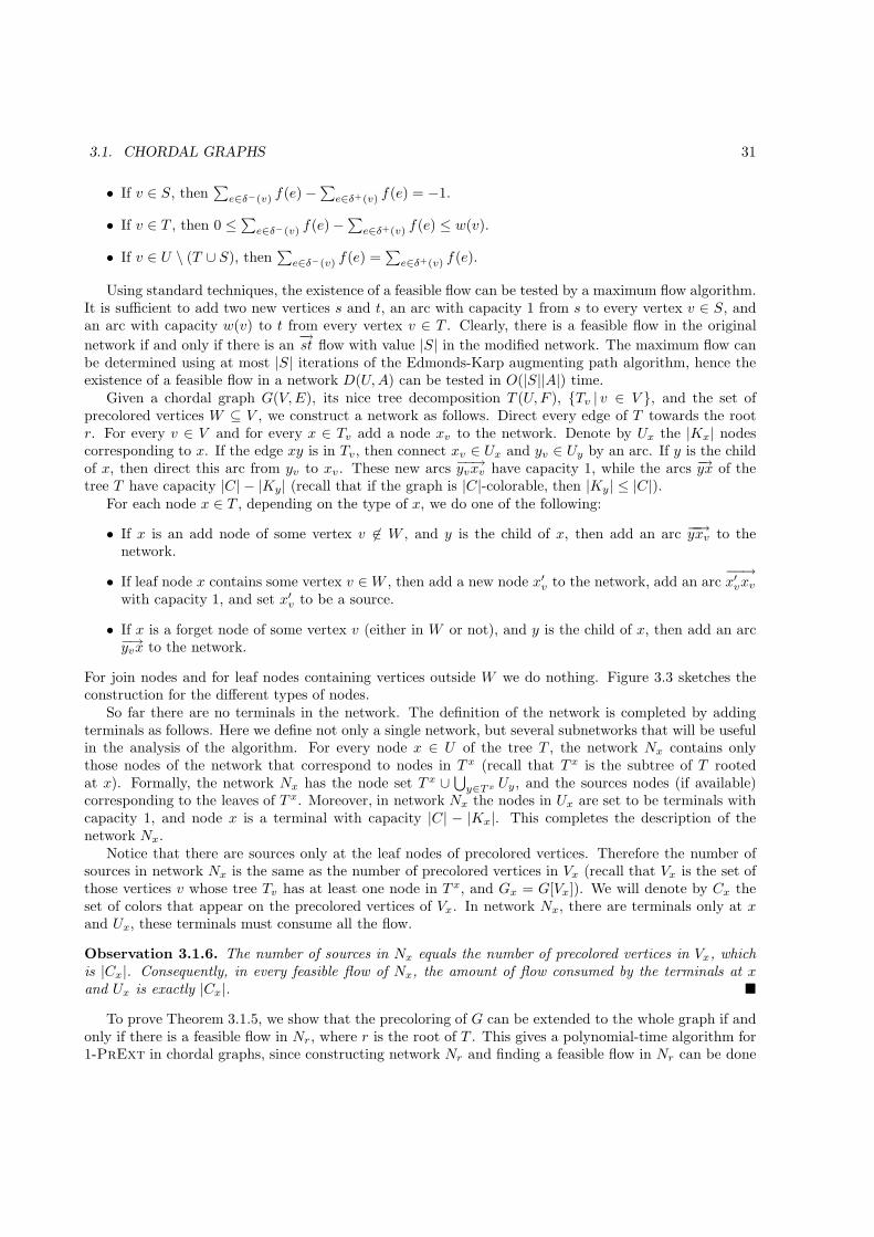
3.1. CHORDAL GRAPHS 31
• If v ∈ S, then∑
e∈δ−(v) f(e) −∑e∈δ+(v) f(e) = −1.
• If v ∈ T , then 0 ≤∑
e∈δ−(v) f(e) −∑
e∈δ+(v) f(e) ≤ w(v).
• If v ∈ U \ (T ∪ S), then∑
e∈δ−(v) f(e) =∑
e∈δ+(v) f(e).
Using standard techniques, the existence of a feasible flow can be tested by a maximum flow algorithm.It is sufficient to add two new vertices s and t, an arc with capacity 1 from s to every vertex v ∈ S, andan arc with capacity w(v) to t from every vertex v ∈ T . Clearly, there is a feasible flow in the original
network if and only if there is an−→st flow with value |S| in the modified network. The maximum flow can
be determined using at most |S| iterations of the Edmonds-Karp augmenting path algorithm, hence theexistence of a feasible flow in a network D(U,A) can be tested in O(|S||A|) time.
Given a chordal graph G(V,E), its nice tree decomposition T (U,F ), {Tv | v ∈ V }, and the set ofprecolored vertices W ⊆ V , we construct a network as follows. Direct every edge of T towards the rootr. For every v ∈ V and for every x ∈ Tv add a node xv to the network. Denote by Ux the |Kx| nodescorresponding to x. If the edge xy is in Tv, then connect xv ∈ Ux and yv ∈ Uy by an arc. If y is the childof x, then direct this arc from yv to xv. These new arcs −−→yvxv have capacity 1, while the arcs −→yx of thetree T have capacity |C| − |Ky| (recall that if the graph is |C|-colorable, then |Ky| ≤ |C|).
For each node x ∈ T , depending on the type of x, we do one of the following:
• If x is an add node of some vertex v 6∈ W , and y is the child of x, then add an arc −−→yxv to thenetwork.
• If leaf node x contains some vertex v ∈W , then add a new node x′v to the network, add an arc−−→x′vxv
with capacity 1, and set x′v to be a source.
• If x is a forget node of some vertex v (either in W or not), and y is the child of x, then add an arc−→yvx to the network.
For join nodes and for leaf nodes containing vertices outside W we do nothing. Figure 3.3 sketches theconstruction for the different types of nodes.
So far there are no terminals in the network. The definition of the network is completed by addingterminals as follows. Here we define not only a single network, but several subnetworks that will be usefulin the analysis of the algorithm. For every node x ∈ U of the tree T , the network Nx contains onlythose nodes of the network that correspond to nodes in T x (recall that T x is the subtree of T rootedat x). Formally, the network Nx has the node set T x ∪
⋃y∈Tx Uy, and the sources nodes (if available)
corresponding to the leaves of T x. Moreover, in network Nx the nodes in Ux are set to be terminals withcapacity 1, and node x is a terminal with capacity |C| − |Kx|. This completes the description of thenetwork Nx.
Notice that there are sources only at the leaf nodes of precolored vertices. Therefore the number ofsources in network Nx is the same as the number of precolored vertices in Vx (recall that Vx is the set ofthose vertices v whose tree Tv has at least one node in T x, and Gx = G[Vx]). We will denote by Cx theset of colors that appear on the precolored vertices of Vx. In network Nx, there are terminals only at xand Ux, these terminals must consume all the flow.
Observation 3.1.6. The number of sources in Nx equals the number of precolored vertices in Vx, whichis |Cx|. Consequently, in every feasible flow of Nx, the amount of flow consumed by the terminals at xand Ux is exactly |Cx|. �
To prove Theorem 3.1.5, we show that the precoloring of G can be extended to the whole graph if andonly if there is a feasible flow in Nr, where r is the root of T . This gives a polynomial-time algorithm for1-PrExt in chordal graphs, since constructing network Nr and finding a feasible flow in Nr can be done
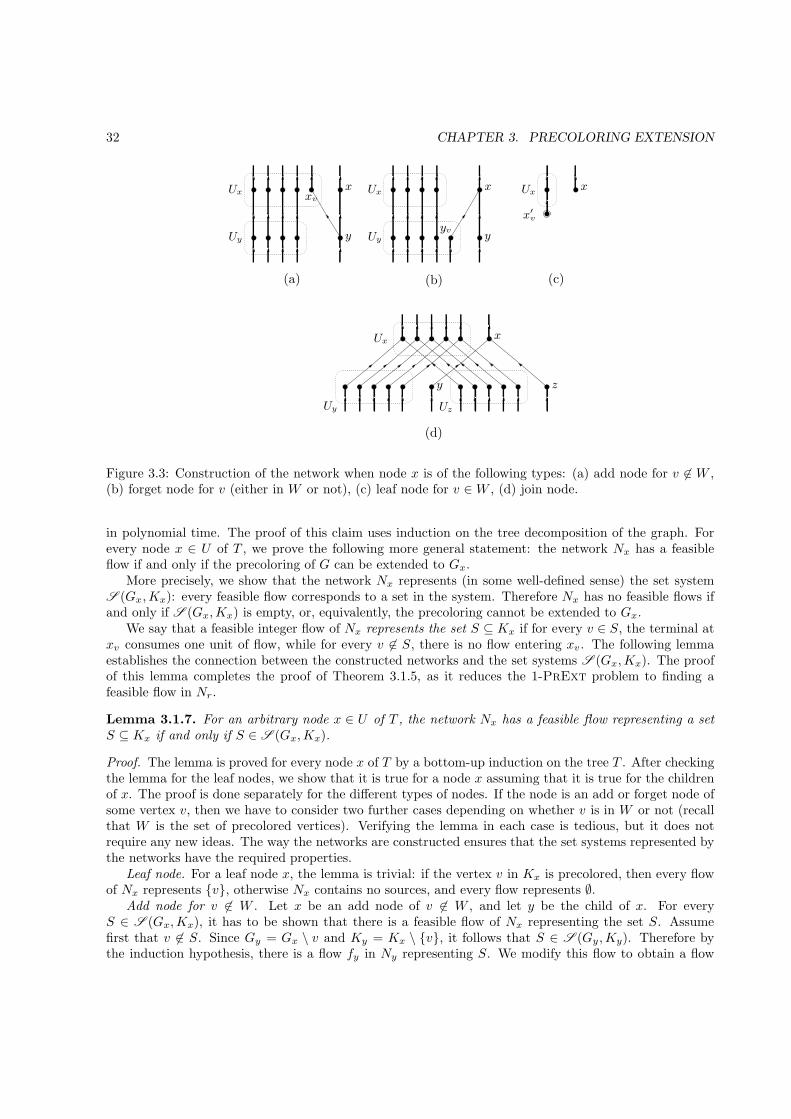
32 CHAPTER 3. PRECOLORING EXTENSION
(a)
x′
v
xv
yv
z
x
xx x
Ux
UxUx Ux
y
yy
Uy
UyUy
Uz
(d)
(c)(b)
Figure 3.3: Construction of the network when node x is of the following types: (a) add node for v 6∈ W ,(b) forget node for v (either in W or not), (c) leaf node for v ∈W , (d) join node.
in polynomial time. The proof of this claim uses induction on the tree decomposition of the graph. Forevery node x ∈ U of T , we prove the following more general statement: the network Nx has a feasibleflow if and only if the precoloring of G can be extended to Gx.
More precisely, we show that the network Nx represents (in some well-defined sense) the set systemS (Gx,Kx): every feasible flow corresponds to a set in the system. Therefore Nx has no feasible flows ifand only if S (Gx,Kx) is empty, or, equivalently, the precoloring cannot be extended to Gx.
We say that a feasible integer flow of Nx represents the set S ⊆ Kx if for every v ∈ S, the terminal atxv consumes one unit of flow, while for every v 6∈ S, there is no flow entering xv. The following lemmaestablishes the connection between the constructed networks and the set systems S (Gx,Kx). The proofof this lemma completes the proof of Theorem 3.1.5, as it reduces the 1-PrExt problem to finding afeasible flow in Nr.
Lemma 3.1.7. For an arbitrary node x ∈ U of T , the network Nx has a feasible flow representing a setS ⊆ Kx if and only if S ∈ S (Gx,Kx).
Proof. The lemma is proved for every node x of T by a bottom-up induction on the tree T . After checkingthe lemma for the leaf nodes, we show that it is true for a node x assuming that it is true for the childrenof x. The proof is done separately for the different types of nodes. If the node is an add or forget node ofsome vertex v, then we have to consider two further cases depending on whether v is in W or not (recallthat W is the set of precolored vertices). Verifying the lemma in each case is tedious, but it does notrequire any new ideas. The way the networks are constructed ensures that the set systems represented bythe networks have the required properties.
Leaf node. For a leaf node x, the lemma is trivial: if the vertex v in Kx is precolored, then every flowof Nx represents {v}, otherwise Nx contains no sources, and every flow represents ∅.
Add node for v 6∈ W . Let x be an add node of v 6∈ W , and let y be the child of x. For everyS ∈ S (Gx,Kx), it has to be shown that there is a feasible flow of Nx representing the set S. Assumefirst that v 6∈ S. Since Gy = Gx \ v and Ky = Kx \ {v}, it follows that S ∈ S (Gy ,Ky). Therefore bythe induction hypothesis, there is a flow fy in Ny representing S. We modify this flow to obtain a flow
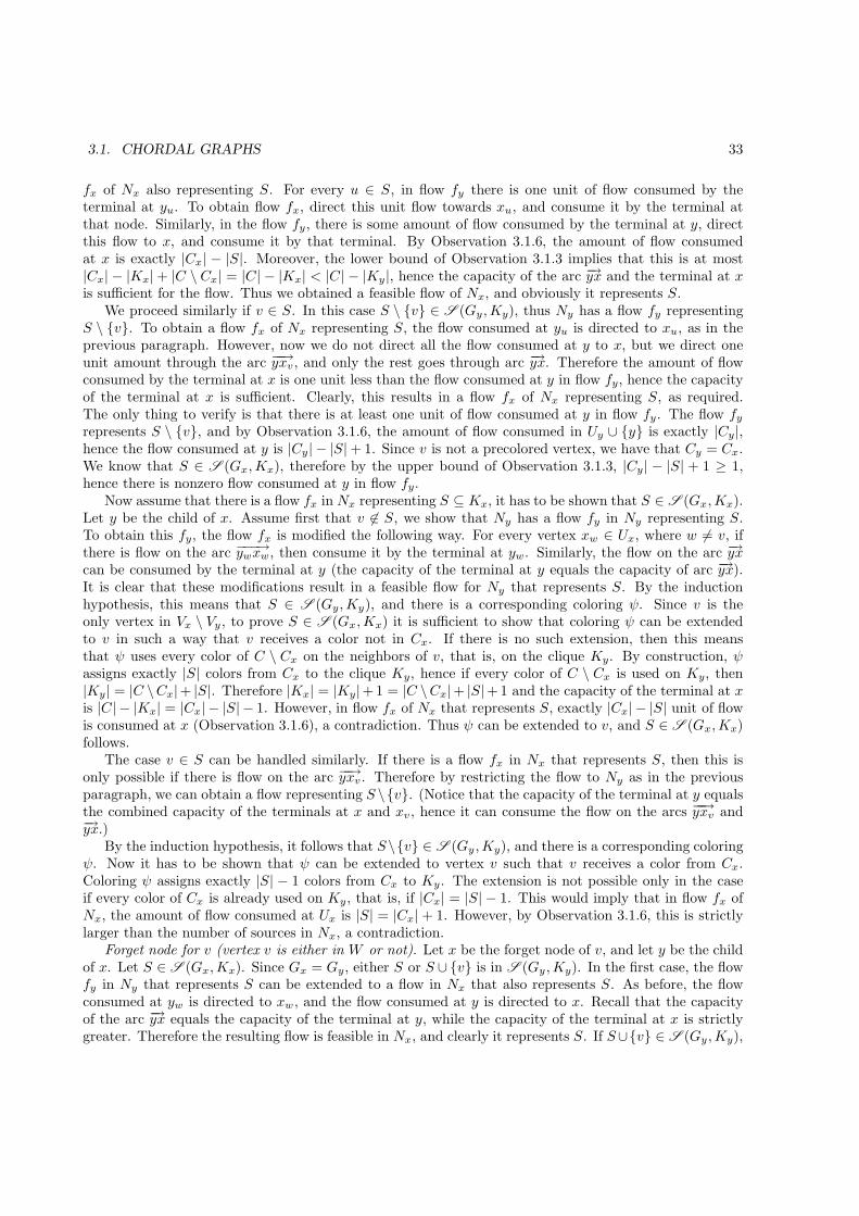
3.1. CHORDAL GRAPHS 33
fx of Nx also representing S. For every u ∈ S, in flow fy there is one unit of flow consumed by theterminal at yu. To obtain flow fx, direct this unit flow towards xu, and consume it by the terminal atthat node. Similarly, in the flow fy, there is some amount of flow consumed by the terminal at y, directthis flow to x, and consume it by that terminal. By Observation 3.1.6, the amount of flow consumedat x is exactly |Cx| − |S|. Moreover, the lower bound of Observation 3.1.3 implies that this is at most|Cx| − |Kx| + |C \ Cx| = |C| − |Kx| < |C| − |Ky|, hence the capacity of the arc −→yx and the terminal at xis sufficient for the flow. Thus we obtained a feasible flow of Nx, and obviously it represents S.
We proceed similarly if v ∈ S. In this case S \ {v} ∈ S (Gy ,Ky), thus Ny has a flow fy representingS \ {v}. To obtain a flow fx of Nx representing S, the flow consumed at yu is directed to xu, as in theprevious paragraph. However, now we do not direct all the flow consumed at y to x, but we direct oneunit amount through the arc −−→yxv, and only the rest goes through arc −→yx. Therefore the amount of flowconsumed by the terminal at x is one unit less than the flow consumed at y in flow fy, hence the capacityof the terminal at x is sufficient. Clearly, this results in a flow fx of Nx representing S, as required.The only thing to verify is that there is at least one unit of flow consumed at y in flow fy. The flow fyrepresents S \ {v}, and by Observation 3.1.6, the amount of flow consumed in Uy ∪ {y} is exactly |Cy|,hence the flow consumed at y is |Cy| − |S| + 1. Since v is not a precolored vertex, we have that Cy = Cx.We know that S ∈ S (Gx,Kx), therefore by the upper bound of Observation 3.1.3, |Cy| − |S| + 1 ≥ 1,hence there is nonzero flow consumed at y in flow fy.
Now assume that there is a flow fx in Nx representing S ⊆ Kx, it has to be shown that S ∈ S (Gx,Kx).Let y be the child of x. Assume first that v 6∈ S, we show that Ny has a flow fy in Ny representing S.To obtain this fy, the flow fx is modified the following way. For every vertex xw ∈ Ux, where w 6= v, ifthere is flow on the arc −−−→ywxw, then consume it by the terminal at yw. Similarly, the flow on the arc −→yxcan be consumed by the terminal at y (the capacity of the terminal at y equals the capacity of arc −→yx).It is clear that these modifications result in a feasible flow for Ny that represents S. By the inductionhypothesis, this means that S ∈ S (Gy,Ky), and there is a corresponding coloring ψ. Since v is theonly vertex in Vx \ Vy , to prove S ∈ S (Gx,Kx) it is sufficient to show that coloring ψ can be extendedto v in such a way that v receives a color not in Cx. If there is no such extension, then this meansthat ψ uses every color of C \ Cx on the neighbors of v, that is, on the clique Ky. By construction, ψassigns exactly |S| colors from Cx to the clique Ky, hence if every color of C \ Cx is used on Ky, then|Ky| = |C \Cx|+ |S|. Therefore |Kx| = |Ky|+ 1 = |C \Cx|+ |S|+ 1 and the capacity of the terminal at xis |C| − |Kx| = |Cx| − |S| − 1. However, in flow fx of Nx that represents S, exactly |Cx| − |S| unit of flowis consumed at x (Observation 3.1.6), a contradiction. Thus ψ can be extended to v, and S ∈ S (Gx,Kx)follows.
The case v ∈ S can be handled similarly. If there is a flow fx in Nx that represents S, then this isonly possible if there is flow on the arc −−→yxv. Therefore by restricting the flow to Ny as in the previousparagraph, we can obtain a flow representing S \{v}. (Notice that the capacity of the terminal at y equalsthe combined capacity of the terminals at x and xv, hence it can consume the flow on the arcs −−→yxv and−→yx.)
By the induction hypothesis, it follows that S\{v} ∈ S (Gy ,Ky), and there is a corresponding coloringψ. Now it has to be shown that ψ can be extended to vertex v such that v receives a color from Cx.Coloring ψ assigns exactly |S| − 1 colors from Cx to Ky. The extension is not possible only in the caseif every color of Cx is already used on Ky, that is, if |Cx| = |S| − 1. This would imply that in flow fx ofNx, the amount of flow consumed at Ux is |S| = |Cx| + 1. However, by Observation 3.1.6, this is strictlylarger than the number of sources in Nx, a contradiction.
Forget node for v (vertex v is either in W or not). Let x be the forget node of v, and let y be the childof x. Let S ∈ S (Gx,Kx). Since Gx = Gy, either S or S ∪ {v} is in S (Gy ,Ky). In the first case, the flowfy in Ny that represents S can be extended to a flow in Nx that also represents S. As before, the flowconsumed at yw is directed to xw , and the flow consumed at y is directed to x. Recall that the capacityof the arc −→yx equals the capacity of the terminal at y, while the capacity of the terminal at x is strictlygreater. Therefore the resulting flow is feasible in Nx, and clearly it represents S. If S∪{v} ∈ S (Gy ,Ky),

34 CHAPTER 3. PRECOLORING EXTENSION
then we do the same, but the flow consumed at yv is directed to x through the arc −→yvx. The resultingflow is feasible in Nx and represents S.
To prove the other direction, assume that Nx has a flow fx representing S ⊆ Kx. Restrict this flow toNy, that is, modify the flow such that the terminals at y and Uy consume all the flow. This results in afeasible flow fy of Ny that represents S or S ∪ {v}. Notice that the terminal at y has the same capacityas the arc −→yx, hence this terminal can consume all the flow going through the arc. Therefore, by theinduction hypothesis, either S or S ∪ {v} is in S (Gy ,Ky), depending on whether there is flow consumedat yv or not. In either case, S ∈ S (Gx,Ky) follows since Gx = Gy and Kx = Ky \ {v}.
Join node. Let y and z be the two children of the join node x. Let S ∈ S (Gx,Kx). By Lemma 3.1.4this means that
|S| ≥ |Kx| − |C \ Cx| (3.1)
and S can be partitioned into disjoint sets S1 ∈ S (Gy,Ky) and S2 ∈ S (Gz ,Kz). By the inductionhypothesis, this implies that there are flows fy, fz in Ny and Nz that represent the sets S1 and S2,respectively. We combine these two flows to obtain a flow fx of Nx that represents the set S. If thereis flow consumed at a node yv ∈ Uy (resp. zv ∈ Uz) in fy (resp. fz), then direct this flow on the arc−−→yvxv (resp. −−→zvxv) to node xv, and consume it there. The capacity of the terminal at xv is 1, but thedisjointness of S1 and S2 implies that at most one unit of flow is directed to xv. The flow consumed atnode y and z is directed to x on the arc −→yx, −→zx, respectively. Since there are exactly |S| units of flowconsumed in Ux, therefore |Cx| − |S| units of flow has to be consumed at x. By (3.1), this is at most|Cx| − |Kx|+ |C \Cx| = |C| − |Kx|, thus the capacity of the terminal at x is sufficient for consuming thisflow. Therefore we have obtained a flow fx in network Nx that represents S.
Now assume that Nx has a flow fx that represents S. Since the terminal at x has capacity at most|C| − |Kx|, and by Observation 3.1.6, the amount of flow consumed in x ∪ Ux is |Cx|, it follows that
|S| ≥ |Cx| − (|C| − |Kx|) = |Kx| − |C \Cx|. (3.2)
If flow is consumed at a node xv ∈ Ux, then the flow arrives to this node either from yv or from zv. Definethe sets S1, S2 ⊆ Kx such that v ∈ S1 (resp. v ∈ S2) if there is flow on arc −−→yvxv (resp. −−→zvxv).
Based on the flow fx of Nx representing S, we create a flow fy of Ny that represents S1 and a flow fz ofNz that represents S2. The flows fy and fz are constructed as follows. For every yv ∈ Uy, if there is flowgoing through the arc −−→yvxv, then consume this flow at yv, and similarly for the nodes zv ∈ Uz. The flowon arcs −→yx and −→zx are consumed at y and z, respectively (the capacity of nodes x, y, and z are the same|C| − |Kx| = |C| − |Ky| = |C| − |Kz|). Clearly, flows fy and fz represent S1 and S2, respectively. By theinduction hypothesis, the flows fx and fy imply that S1 ∈ S (Gy,Ky) and S2 ∈ S (Gz ,Kz). Furthermore,it is clear that S1 and S2 are disjoint, and S = S1 ∪ S2. Therefore by Lemma 3.1.4 and Inequality (3.2),this proves that S ∈ S (Gx,Kx), as required.
�
To determine the running time of the algorithm, we have to consider two main steps: the constructionof the network and the solution of the flow problem. First of all, the transformation introduced at theend of Section 3.1.1 can increase the size of the graph by at most a factor of n. Given a chordal graphG(V,E), its tree decomposition can be constructed by first finding a perfect vertex elimination scheme[Gol80, RTL76]. Based on this ordering of the vertices, one can build a tree T (U,F ) of size |V |, and onesubtree for each vertex of the graph. This tree decomposition can be found in time linear in the size ofthe output, that is, in O(|V |2) time. Converting T (U,F ) to a nice tree decomposition can introduce anincrease of factor at most |V |, thus it can be done in O(|V |3) time. The network defined by the algorithmhas size linear in the total size of the tree decomposition (size of T (U,F ) and the sum of the size of thesubtrees), and clearly it can be constructed in linear time. Therefore the constructed network has O(|V |3)nodes and O(|V |3) arcs, and the construction takes O(|V |3) time.
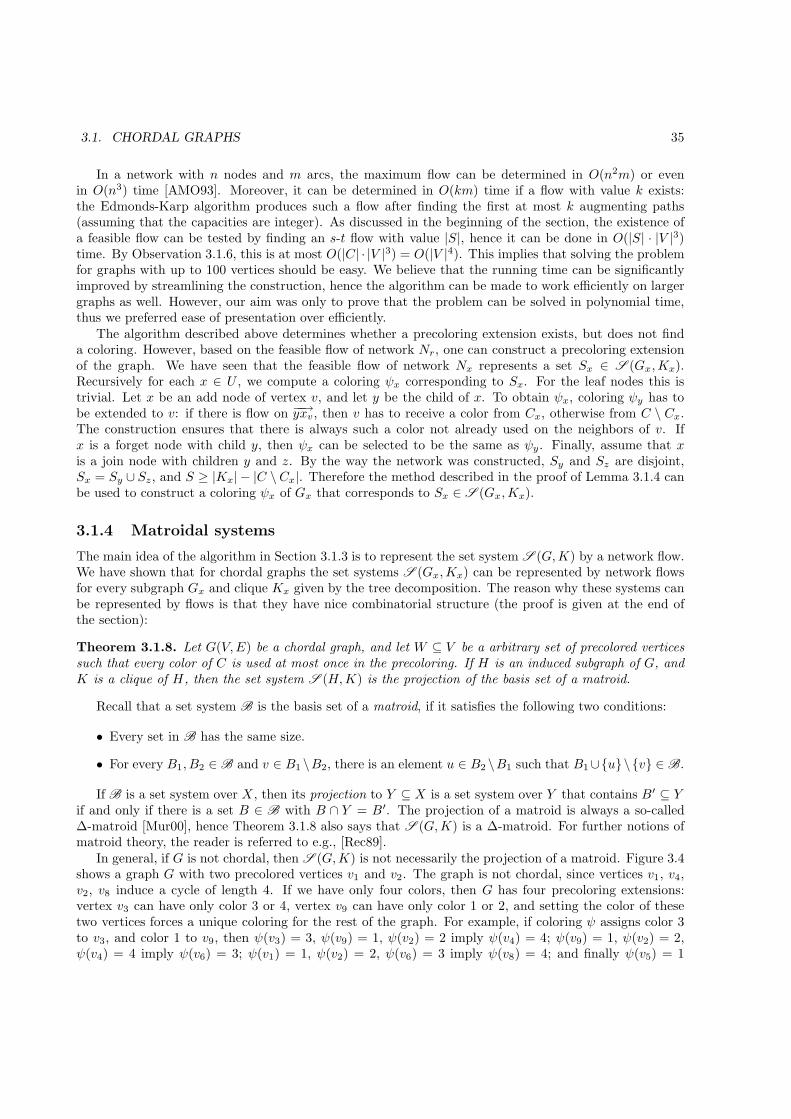
3.1. CHORDAL GRAPHS 35
In a network with n nodes and m arcs, the maximum flow can be determined in O(n2m) or evenin O(n3) time [AMO93]. Moreover, it can be determined in O(km) time if a flow with value k exists:the Edmonds-Karp algorithm produces such a flow after finding the first at most k augmenting paths(assuming that the capacities are integer). As discussed in the beginning of the section, the existence ofa feasible flow can be tested by finding an s-t flow with value |S|, hence it can be done in O(|S| · |V |3)time. By Observation 3.1.6, this is at most O(|C| · |V |3) = O(|V |4). This implies that solving the problemfor graphs with up to 100 vertices should be easy. We believe that the running time can be significantlyimproved by streamlining the construction, hence the algorithm can be made to work efficiently on largergraphs as well. However, our aim was only to prove that the problem can be solved in polynomial time,thus we preferred ease of presentation over efficiently.
The algorithm described above determines whether a precoloring extension exists, but does not finda coloring. However, based on the feasible flow of network Nr, one can construct a precoloring extensionof the graph. We have seen that the feasible flow of network Nx represents a set Sx ∈ S (Gx,Kx).Recursively for each x ∈ U , we compute a coloring ψx corresponding to Sx. For the leaf nodes this istrivial. Let x be an add node of vertex v, and let y be the child of x. To obtain ψx, coloring ψy has tobe extended to v: if there is flow on −−→yxv, then v has to receive a color from Cx, otherwise from C \ Cx.The construction ensures that there is always such a color not already used on the neighbors of v. Ifx is a forget node with child y, then ψx can be selected to be the same as ψy. Finally, assume that xis a join node with children y and z. By the way the network was constructed, Sy and Sz are disjoint,Sx = Sy ∪ Sz, and S ≥ |Kx| − |C \Cx|. Therefore the method described in the proof of Lemma 3.1.4 canbe used to construct a coloring ψx of Gx that corresponds to Sx ∈ S (Gx,Kx).
3.1.4 Matroidal systems
The main idea of the algorithm in Section 3.1.3 is to represent the set system S (G,K) by a network flow.We have shown that for chordal graphs the set systems S (Gx,Kx) can be represented by network flowsfor every subgraph Gx and clique Kx given by the tree decomposition. The reason why these systems canbe represented by flows is that they have nice combinatorial structure (the proof is given at the end ofthe section):
Theorem 3.1.8. Let G(V,E) be a chordal graph, and let W ⊆ V be a arbitrary set of precolored verticessuch that every color of C is used at most once in the precoloring. If H is an induced subgraph of G, andK is a clique of H, then the set system S (H,K) is the projection of the basis set of a matroid.
Recall that a set system B is the basis set of a matroid, if it satisfies the following two conditions:
• Every set in B has the same size.
• For every B1, B2 ∈ B and v ∈ B1 \B2, there is an element u ∈ B2 \B1 such that B1∪{u}\{v} ∈ B.
If B is a set system over X , then its projection to Y ⊆ X is a set system over Y that contains B′ ⊆ Yif and only if there is a set B ∈ B with B ∩ Y = B′. The projection of a matroid is always a so-called∆-matroid [Mur00], hence Theorem 3.1.8 also says that S (G,K) is a ∆-matroid. For further notions ofmatroid theory, the reader is referred to e.g., [Rec89].
In general, if G is not chordal, then S (G,K) is not necessarily the projection of a matroid. Figure 3.4shows a graph G with two precolored vertices v1 and v2. The graph is not chordal, since vertices v1, v4,v2, v8 induce a cycle of length 4. If we have only four colors, then G has four precoloring extensions:vertex v3 can have only color 3 or 4, vertex v9 can have only color 1 or 2, and setting the color of thesetwo vertices forces a unique coloring for the rest of the graph. For example, if coloring ψ assigns color 3to v3, and color 1 to v9, then ψ(v3) = 3, ψ(v9) = 1, ψ(v2) = 2 imply ψ(v4) = 4; ψ(v9) = 1, ψ(v2) = 2,ψ(v4) = 4 imply ψ(v6) = 3; ψ(v1) = 1, ψ(v2) = 2, ψ(v6) = 3 imply ψ(v8) = 4; and finally ψ(v5) = 1
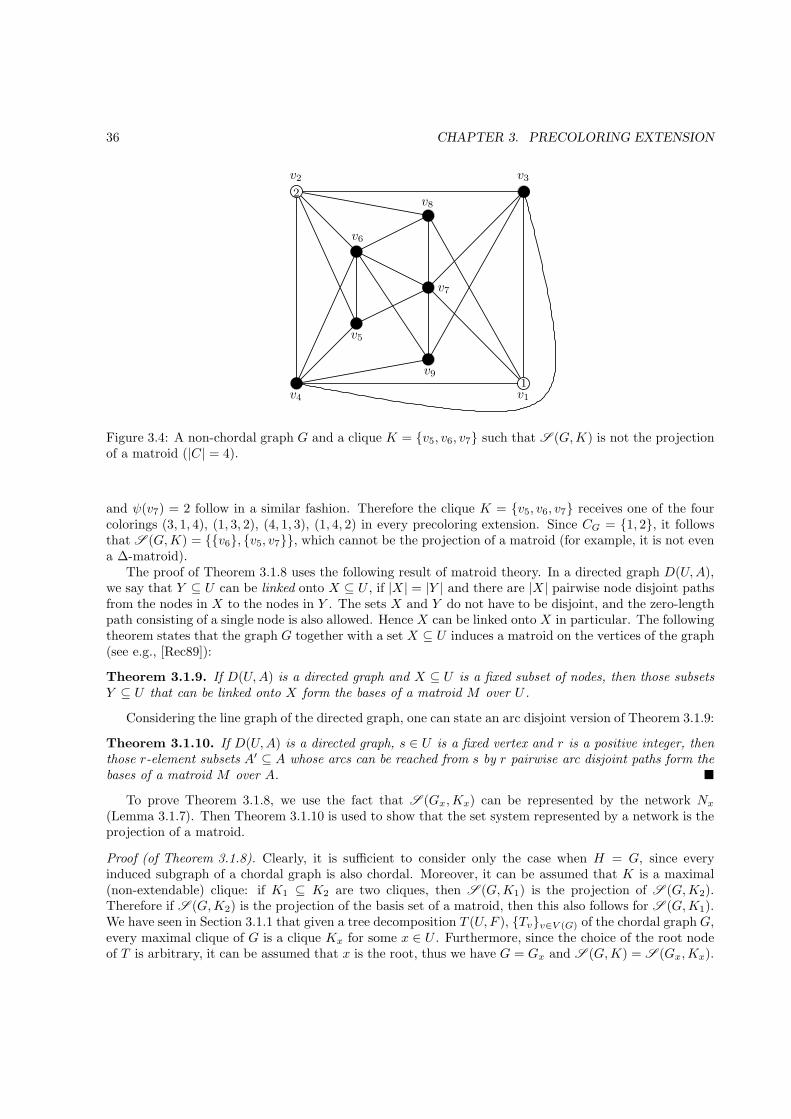
36 CHAPTER 3. PRECOLORING EXTENSION
v4
v5
v6
v2 v3
v1
v8
v9
v7
1
2
Figure 3.4: A non-chordal graph G and a clique K = {v5, v6, v7} such that S (G,K) is not the projectionof a matroid (|C| = 4).
and ψ(v7) = 2 follow in a similar fashion. Therefore the clique K = {v5, v6, v7} receives one of the fourcolorings (3, 1, 4), (1, 3, 2), (4, 1, 3), (1, 4, 2) in every precoloring extension. Since CG = {1, 2}, it followsthat S (G,K) = {{v6}, {v5, v7}}, which cannot be the projection of a matroid (for example, it is not evena ∆-matroid).
The proof of Theorem 3.1.8 uses the following result of matroid theory. In a directed graph D(U,A),we say that Y ⊆ U can be linked onto X ⊆ U , if |X | = |Y | and there are |X | pairwise node disjoint pathsfrom the nodes in X to the nodes in Y . The sets X and Y do not have to be disjoint, and the zero-lengthpath consisting of a single node is also allowed. Hence X can be linked onto X in particular. The followingtheorem states that the graph G together with a set X ⊆ U induces a matroid on the vertices of the graph(see e.g., [Rec89]):
Theorem 3.1.9. If D(U,A) is a directed graph and X ⊆ U is a fixed subset of nodes, then those subsetsY ⊆ U that can be linked onto X form the bases of a matroid M over U .
Considering the line graph of the directed graph, one can state an arc disjoint version of Theorem 3.1.9:
Theorem 3.1.10. If D(U,A) is a directed graph, s ∈ U is a fixed vertex and r is a positive integer, thenthose r-element subsets A′ ⊆ A whose arcs can be reached from s by r pairwise arc disjoint paths form thebases of a matroid M over A. �
To prove Theorem 3.1.8, we use the fact that S (Gx,Kx) can be represented by the network Nx(Lemma 3.1.7). Then Theorem 3.1.10 is used to show that the set system represented by a network is theprojection of a matroid.
Proof (of Theorem 3.1.8). Clearly, it is sufficient to consider only the case when H = G, since everyinduced subgraph of a chordal graph is also chordal. Moreover, it can be assumed that K is a maximal(non-extendable) clique: if K1 ⊆ K2 are two cliques, then S (G,K1) is the projection of S (G,K2).Therefore if S (G,K2) is the projection of the basis set of a matroid, then this also follows for S (G,K1).We have seen in Section 3.1.1 that given a tree decomposition T (U,F ), {Tv}v∈V (G) of the chordal graph G,every maximal clique of G is a clique Kx for some x ∈ U . Furthermore, since the choice of the root nodeof T is arbitrary, it can be assumed that x is the root, thus we have G = Gx and S (G,K) = S (Gx,Kx).
3.1. CHORDAL GRAPHS 37
By Lemma 3.1.7, the sets in S (Gx,Kx) are exactly the sets represented by the feasible flows of thenetwork Nx. Now, as described at the beginning of Section 3.1.3, add two new nodes s, t to the network,add an arc with unit capacity from s to every source, and for every terminal x, add an arc from x to t thathas capacity equal to the capacity of x. Furthermore, replace every arc e having capacity c(e) with c(e)parallel arcs of unit capacity, clearly this does not change the problem. Call the resulting network N ′
x. ByObservation 3.1.6, the number of sources in Nx is r = |Cx|, hence every feasible flow of Nx corresponds
to an−→st flow with value r in N ′
x. Since every arc has unit capacity in N ′x, an integral
−→st flow with value
r corresponds to r arc disjoint paths from s to t. Now consider the matroid M given by Lemma 3.1.10.Denote by At the arcs incident to t, and let matroid Mt be the restriction of matroid M to At. LetA′t ⊆ At be those arcs of At that originate from some node xv ∈ Ux (and not from x). We claim that
S (G,Kx) is isomorphic to the projection of Mt to A′t (vertex v ∈ Kx maps to arc
−→xvt). By Lemma 3.1.7,
if S ∈ S (G,Kx), then there is a feasible flow in Nx where flow is consumed only by those terminals of
Ux that correspond to the elements in S. Based on this flow, one can find r arc disjoint−→st paths in N ′
x,and it follows that the matroid Mt has a base whose intersection with A′
t is exactly S, hence S is in theprojection of Mt to A′
t. It is easy to show the other direction as well: if S is in the projection of Mt, thenthere is a feasible flow of Nx where only the terminals corresponding to S consume flow in Ux. Thus byLemma 3.1.7, S ∈ S (G,Kx), as required. �
3.1.5 Applications
A possible application area for Theorem 3.1.5 is the design and configuration of Wavelength DivisionMultiplexing (WDM) optical networks. WDM technology allows us to establish several data channels ina single optical fiber using the different wavelengths. All-optical switches can route the different channelsof an incoming fiber to different outgoing fibers. Therefore by configuring the switches appropriately,we can create direct optical connections between distant nodes of the network. However, in order toconfigure the network, we have to assign a wavelength to each connection such that connections that usethe same fiber receive different wavelengths. This wavelength assignment problem is a coloring problem.The conflict graph of the network has one vertex for each connection, and two vertices are neighbors ifthe corresponding two connections share a fiber. If the number of wavelengths in a fiber is k, then thewavelength assignment problem can be solved if and only if the conflict graph is k-colorable.
The WDM network configuration problem was studied by several papers in the literature, with aparticular emphasis on tree and tree-like networks [EJ01, Erl99, EJK+99, EJ98, ART01]. However, themodel becomes slightly different if we consider another type of optical switches. The simplest opticalswitch is the passive star that selects one incoming fiber for each wavelength, and transmits the data onthis wavelength to every outgoing fiber. If we have this type of switches, then connections having the samewavelength cannot go through the same switch. That is, the connections with the same wavelength haveto be vertex disjoint, not only edge disjoint. We can take into account this restriction by modifying thedefinition of the conflict graph: connect those vertices where the corresponding connections go through thesame switch. As discussed in Section 3.1.1, the intersection graph of paths in a tree is always chordal, hencethe conflict graph in this problem will be a chordal graph. Vertex coloring is polynomial-time solvable forchordal graphs, hence we can determine in polynomial time whether the wavelength assignment problemcan be solved. The algorithm in Theorem 3.1.5 gives a method for solving the slightly more generalproblem where some of the connections already have a wavelength, but every wavelength is assigned to atmost one connection. For example, this is the case if all the connections going through a particular switchare already assigned a wavelength, but we are free to assign any wavelength to the remaining connections.
We remark that with chordal graphs we can model a more general problem as well. The intersectiongraph of the subtrees in tree gives a chordal graph, thus if the connections are not paths but trees, thenthe same method works. This observation might be useful if we have to establish broadcast connectionsbetween multiple parties.
38 CHAPTER 3. PRECOLORING EXTENSION
3.2 The Eulerian disjoint paths problem
Disjoint paths problems arise naturally in practical applications such as network routing and VLSI-design.The problem is also interesting from the theoretical point of view: there are several beautiful goodcharacterization theorems for some restricted cases. The restriction to planar graphs, and in particularto planar grid graphs is both of practical and theoretical interest. Here we prove the NP-completeness ofa planar case of the problem, settling an open question of Vygen [Vyg94]. This complements the goodcharacterization theorem of Okamura and Seymour. Moreover, this result will be used in Section 3.3 toprove the NP-completeness of precoloring extension on unit interval graphs.
In the disjoint paths problem we are given a graph G and a set of source–destination pairs (s1, t1),(s2, t2), . . . , (sk, tk) called the terminals, and we have to find k disjoint paths P1, . . . , Pk such that pathPi connects vertex si to vertex ti. There are four basic variants of the problem: the graph can be directedor undirected, and we can require edge disjoint or vertex disjoint paths. The problem is often describedin terms of a supply graph and a demand graph, as follows:
Disjoint Paths
Input: The supply graph G and the demand graph H on the same set of vertices.
Task: Find a path Pe in G for each e ∈ E(H) such that these paths are pairwise disjoint andpath Pe together with edge e forms a circuit.
The graphs G and H can have parallel edges but no loops. For vertex disjoint paths we allow theirendpoints to be the same. In the directed version of the problem both G and H are directed. With aslight abuse of terminology, we say in the directed case that a demand −→uv ∈ H starts in v and ends inu (since the directed path satisfying this demand starts in v and ends in u). Moreover, given a solutionof the disjoint paths problem, we identify a demand with the path satisfying it. That is, we say that“demand α uses supply edge e” instead of “the path satisfying demand α uses edge e”. An undirectedgraph is called Eulerian if every vertex has even degree, and a directed graph is Eulerian if the indegreeequals the outdegree at every vertex.
The disjoint paths problem and its variants were intensively studied, for an overview see [Fra90, Vyg94].In particular, all four variants of the problem (directed/undirected, edge disjoint/vertex disjoint) are NP-complete, even when G is planar. In this paper we consider only the (directed and undirected) edgedisjoint paths problem in the grid, thus henceforth disjoint means edge disjoint.
If there exist disjoint paths in G(V,E) with the given endpoints, then every cut (V ′, V \ V ′) has tocontain at least as many edges from G as from H , otherwise there would be more demands crossing thiscut than edges connecting V ′ and V \ V ′. We say that the cut criterion holds for G and H if this is truefor every cut (V ′, V \ V ′). In general, the cut criterion is only a necessary condition, but in an importantspecial case it is also sufficient:
Theorem 3.2.1 (Okamura and Seymour, 1981, [OS81]). Assume that G is planar, undirected,G+H is Eulerian, and every edge of H lies on the outer face of G. The edge disjoint paths problem hasa solution if and only if the cut criterion is satisfied.
A graph is a grid graph if it is a finite subgraph of the rectangular grid. A directed grid graph is agrid graph with the horizontal edges directed to the right and the vertical edges directed to the bottom.Clearly, every directed grid graph is acyclic. A rectangle is a grid graph with n × m nodes such thatvi,j (1 ≤ i ≤ n, 1 ≤ j ≤ m) is connected to vi′,j′ if and only if |i − i′| = 1 and j = j′, or i = i′ and|j − j′| = 1. The study of grid and rectangle graphs is motivated by applications in VLSI-layout.
The special case of Theorem 3.2.1 when G is a rectangle is investigated in [Fra82]. The requirementthat the edges of H lie on the outer face of G cannot be dropped even in this restricted case: Figure 3.5shows an example where G+H is Eulerian, the cut criterion holds, but the terminals cannot be connected
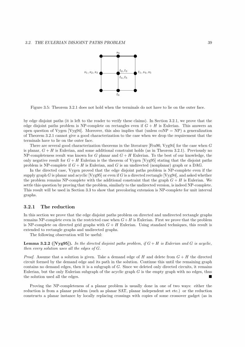
3.2. THE EULERIAN DISJOINT PATHS PROBLEM 39
t2, t3
t4, t5
s6
t6
s1, s2, s3 t1, s4, s5
Figure 3.5: Theorem 3.2.1 does not hold when the terminals do not have to lie on the outer face.
by edge disjoint paths (it is left to the reader to verify these claims). In Section 3.2.1, we prove that theedge disjoint paths problem is NP-complete on rectangles even if G + H is Eulerian. This answers anopen question of Vygen [Vyg94]. Moreover, this also implies that (unless coNP = NP) a generalizationof Theorem 3.2.1 cannot give a good characterization to the case when we drop the requirement that theterminals have to lie on the outer face.
There are several good characterization theorems in the literature [Fra90, Vyg94] for the case when Gis planar, G + H is Eulerian, and some additional constraint holds (as in Theorem 3.2.1). Previously noNP-completeness result was known for G planar and G+H Eulerian. To the best of our knowledge, theonly negative result for G + H Eulerian is the theorem of Vygen [Vyg95] stating that the disjoint pathsproblem is NP-complete if G+H is Eulerian, and G is an undirected (nonplanar) graph or a DAG.
In the directed case, Vygen proved that the edge disjoint paths problem is NP-complete even if thesupply graphG is planar and acyclic [Vyg95] or even if G is a directed rectangle [Vyg94], and asked whetherthe problem remains NP-complete with the additional constraint that the graph G + H is Eulerian. Wesettle this question by proving that the problem, similarly to the undirected version, is indeed NP-complete.This result will be used in Section 3.3 to show that precoloring extension is NP-complete for unit intervalgraphs.
3.2.1 The reduction
In this section we prove that the edge disjoint paths problem on directed and undirected rectangle graphsremains NP-complete even in the restricted case when G+H is Eulerian. First we prove that the problemis NP-complete on directed grid graphs with G + H Eulerian. Using standard techniques, this result isextended to rectangle graphs and undirected graphs.
The following observation will be useful:
Lemma 3.2.2 ([Vyg95]). In the directed disjoint paths problem, if G+H is Eulerian and G is acyclic,then every solution uses all the edges of G.
Proof. Assume that a solution is given. Take a demand edge of H and delete from G + H the directedcircuit formed by the demand edge and its path in the solution. Continue this until the remaining graphcontains no demand edges, then it is a subgraph of G. Since we deleted only directed circuits, it remainsEulerian, but the only Eulerian subgraph of the acyclic graph G is the empty graph with no edges, thusthe solution used all the edges. �
Proving the NP-completeness of a planar problem is usually done in one of two ways: either thereduction is from a planar problem (such as planar SAT, planar independent set etc.) or the reductionconstructs a planar instance by locally replacing crossings with copies of some crossover gadget (as in
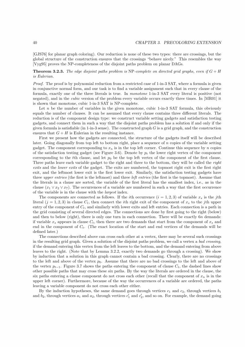
40 CHAPTER 3. PRECOLORING EXTENSION
[GJS76] for planar graph coloring). Our reduction is none of these two types: there are crossings, but theglobal structure of the construction ensures that the crossings “behave nicely.” This resembles the way[Vyg95] proves the NP-completeness of the disjoint paths problem on planar DAGs.
Theorem 3.2.3. The edge disjoint paths problem is NP-complete on directed grid graphs, even if G+His Eulerian.
Proof. The proof is by polynomial reduction from a restricted case of 1-in-3 SAT, where a formula is givenin conjunctive normal form, and our task is to find a variable assignment such that in every clause of theformula, exactly one of the three literals is true. In monotone 1-in-3 SAT every literal is positive (notnegated), and in the cubic version of the problem every variable occurs exactly three times. In [MR01] itis shown that monotone, cubic 1-in-3 SAT is NP-complete.
Let n be the number of variables in the given monotone, cubic 1-in-3 SAT formula, this obviouslyequals the number of clauses. It can be assumed that every clause contains three different literals. Thereduction is of the component design type: we construct variable setting gadgets and satisfaction testinggadgets, and connect them in such a way that the disjoint paths problem has a solution if and only if thegiven formula is satisfiable (in 1-in-3 sense). The constructed graph G is a grid graph, and the constructionensures that G+H is Eulerian in the resulting instance.
First we present how the gadgets are connected, the structure of the gadgets itself will be describedlater. Going diagonally from top left to bottom right, place a sequence of n copies of the variable settinggadget. The component corresponding to xn is in the top left corner. Continue this sequence by n copiesof the satisfaction testing gadget (see Figure 3.6). Denote by pt the lower right vertex of the componentcorresponding to the tth clause, and let p0 be the top left vertex of the component of the first clause.Three paths leave each variable gadget to the right and three to the bottom, they will be called the rightexits and the lower exits of the gadget. The exits are numbered, the topmost right exit is the first rightexit, and the leftmost lower exit is the first lower exit. Similarly, the satisfaction testing gadgets havethree upper entries (the first is the leftmost) and three left entries (the first is the topmost). Assume thatthe literals in a clause are sorted, the variable of the first literal has the smallest index, i.e., as in theclause (x1 ∨ x2 ∨ x7). The occurrences of a variable are numbered in such a way that the first occurrenceof the variable is in the clause with the largest index.
The components are connected as follows. If the ith occurrence (i = 1, 2, 3) of variable xs is the jthliteral (j = 1, 2, 3) in clause Ct, then connect the ith right exit of the component of xs to the jth upperentry of the component of Ct, and similarly with lower exits and left entries. Each connection is a path inthe grid consisting of several directed edges. The connections are done by first going to the right (below)and then to below (right), there is only one turn in each connection. There will be exactly 6n demands:if variable xs appears in clause Ct, then there are two demands that start from the component of xs andend in the component of Ct. (The exact location of the start and end vertices of the demands will bedefined later.)
The connections described above can cross each other at a vertex, there may be several such crossingsin the resulting grid graph. Given a solution of the disjoint paths problem, we call a vertex a bad crossing,if the demand entering this vertex from the left leaves to the bottom, and the demand entering from aboveleaves to the right. (Note that by Lemma 3.2.2, exactly two demands go through a crossing). We showby induction that a solution in this graph cannot contain a bad crossing. Clearly, there are no crossingsto the left and above of the vertex p0. Assume that there are no bad crossings to the left and above ofthe vertex pt−1. Figure 3.7 shows the paths entering the component of clause Ct, the dashed lines showother possible paths that may cross these six paths. By the way the literals are ordered in the clause, thesix paths entering a clause component do not cross each other (recall that the component of xn is in theupper left corner). Furthermore, because of the way the occurrences of a variable are ordered, the pathsleaving a variable component do not cross each other either.
By the induction hypotheses, the same demand goes through vertices c1 and c2, through vertices b1and b2, through vertices a1 and a2, through vertices c′1 and c′2, and so on. For example, the demand going
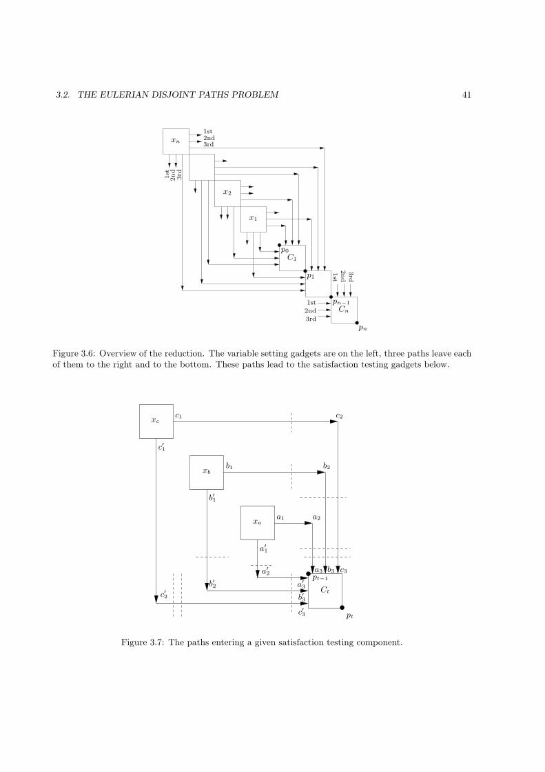
3.2. THE EULERIAN DISJOINT PATHS PROBLEM 41
p1
pn−1
pn
p0
x1
Cn
C1
xn
x2
3rd
3rd
3rd
2nd
2nd
2nd
1st
1st
1st
2nd3rd
1st
Figure 3.6: Overview of the reduction. The variable setting gadgets are on the left, three paths leave eachof them to the right and to the bottom. These paths lead to the satisfaction testing gadgets below.
Ct
pt
pt−1
c′3
b′3
a′3
a′2
b′2c′2
a′1
c′1
b′1
c3b3a3
a2
b2
c2
a1
b1
c1xc
xb
xa
Figure 3.7: The paths entering a given satisfaction testing component.
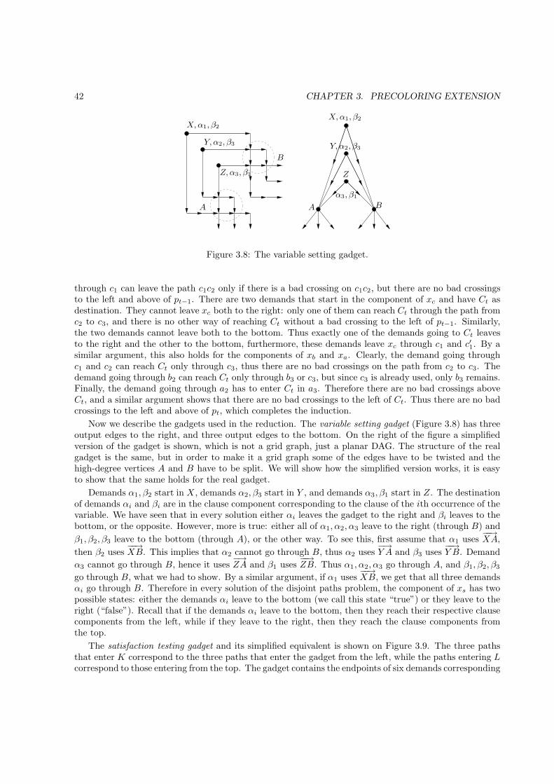
42 CHAPTER 3. PRECOLORING EXTENSION
α3, β1
Y, α2, β3
X,α1, β2
B
B
Z,α3, β1
Y, α2, β3
X,α1, β2
A A
Z
Figure 3.8: The variable setting gadget.
through c1 can leave the path c1c2 only if there is a bad crossing on c1c2, but there are no bad crossingsto the left and above of pt−1. There are two demands that start in the component of xc and have Ct asdestination. They cannot leave xc both to the right: only one of them can reach Ct through the path fromc2 to c3, and there is no other way of reaching Ct without a bad crossing to the left of pt−1. Similarly,the two demands cannot leave both to the bottom. Thus exactly one of the demands going to Ct leavesto the right and the other to the bottom, furthermore, these demands leave xc through c1 and c′1. By asimilar argument, this also holds for the components of xb and xa. Clearly, the demand going throughc1 and c2 can reach Ct only through c3, thus there are no bad crossings on the path from c2 to c3. Thedemand going through b2 can reach Ct only through b3 or c3, but since c3 is already used, only b3 remains.Finally, the demand going through a2 has to enter Ct in a3. Therefore there are no bad crossings aboveCt, and a similar argument shows that there are no bad crossings to the left of Ct. Thus there are no badcrossings to the left and above of pt, which completes the induction.
Now we describe the gadgets used in the reduction. The variable setting gadget (Figure 3.8) has threeoutput edges to the right, and three output edges to the bottom. On the right of the figure a simplifiedversion of the gadget is shown, which is not a grid graph, just a planar DAG. The structure of the realgadget is the same, but in order to make it a grid graph some of the edges have to be twisted and thehigh-degree vertices A and B have to be split. We will show how the simplified version works, it is easyto show that the same holds for the real gadget.
Demands α1, β2 start in X , demands α2, β3 start in Y , and demands α3, β1 start in Z. The destinationof demands αi and βi are in the clause component corresponding to the clause of the ith occurrence of thevariable. We have seen that in every solution either αi leaves the gadget to the right and βi leaves to thebottom, or the opposite. However, more is true: either all of α1, α2, α3 leave to the right (through B) and
β1, β2, β3 leave to the bottom (through A), or the other way. To see this, first assume that α1 uses−−→XA,
then β2 uses−−→XB. This implies that α2 cannot go through B, thus α2 uses
−→Y A and β3 uses
−−→Y B. Demand
α3 cannot go through B, hence it uses−→ZA and β1 uses
−−→ZB. Thus α1, α2, α3 go through A, and β1, β2, β3
go through B, what we had to show. By a similar argument, if α1 uses−−→XB, we get that all three demands
αi go through B. Therefore in every solution of the disjoint paths problem, the component of xs has twopossible states: either the demands αi leave to the bottom (we call this state “true”) or they leave to theright (“false”). Recall that if the demands αi leave to the bottom, then they reach their respective clausecomponents from the left, while if they leave to the right, then they reach the clause components fromthe top.
The satisfaction testing gadget and its simplified equivalent is shown on Figure 3.9. The three pathsthat enter K correspond to the three paths that enter the gadget from the left, while the paths entering Lcorrespond to those entering from the top. The gadget contains the endpoints of six demands corresponding
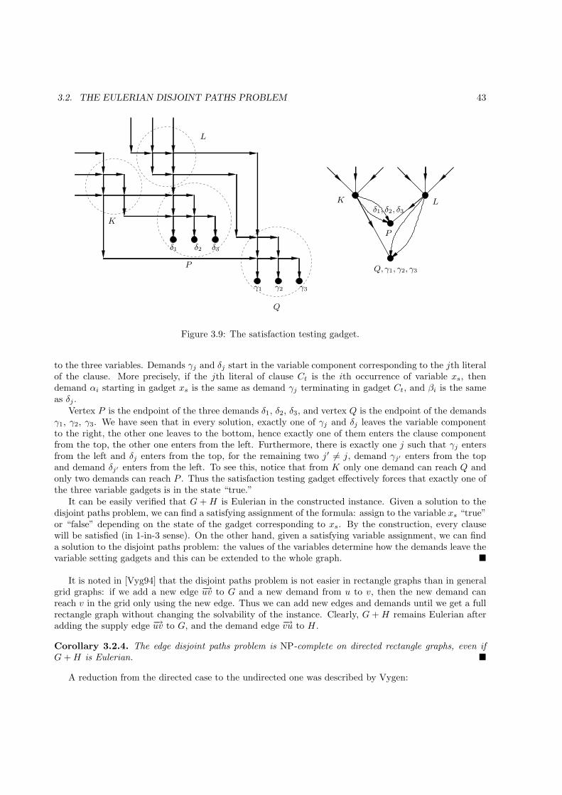
3.2. THE EULERIAN DISJOINT PATHS PROBLEM 43
Q
Q,γ1, γ2, γ3
δ1, δ2, δ3
γ3γ2γ1
δ3δ1 δ2
K L
L
K
P
P
Figure 3.9: The satisfaction testing gadget.
to the three variables. Demands γj and δj start in the variable component corresponding to the jth literalof the clause. More precisely, if the jth literal of clause Ct is the ith occurrence of variable xs, thendemand αi starting in gadget xs is the same as demand γj terminating in gadget Ct, and βi is the sameas δj .
Vertex P is the endpoint of the three demands δ1, δ2, δ3, and vertex Q is the endpoint of the demandsγ1, γ2, γ3. We have seen that in every solution, exactly one of γj and δj leaves the variable componentto the right, the other one leaves to the bottom, hence exactly one of them enters the clause componentfrom the top, the other one enters from the left. Furthermore, there is exactly one j such that γj entersfrom the left and δj enters from the top, for the remaining two j′ 6= j, demand γj′ enters from the topand demand δj′ enters from the left. To see this, notice that from K only one demand can reach Q andonly two demands can reach P . Thus the satisfaction testing gadget effectively forces that exactly one ofthe three variable gadgets is in the state “true.”
It can be easily verified that G + H is Eulerian in the constructed instance. Given a solution to thedisjoint paths problem, we can find a satisfying assignment of the formula: assign to the variable xs “true”or “false” depending on the state of the gadget corresponding to xs. By the construction, every clausewill be satisfied (in 1-in-3 sense). On the other hand, given a satisfying variable assignment, we can finda solution to the disjoint paths problem: the values of the variables determine how the demands leave thevariable setting gadgets and this can be extended to the whole graph. �
It is noted in [Vyg94] that the disjoint paths problem is not easier in rectangle graphs than in generalgrid graphs: if we add a new edge −→uv to G and a new demand from u to v, then the new demand canreach v in the grid only using the new edge. Thus we can add new edges and demands until we get a fullrectangle graph without changing the solvability of the instance. Clearly, G + H remains Eulerian afteradding the supply edge −→uv to G, and the demand edge −→vu to H .
Corollary 3.2.4. The edge disjoint paths problem is NP-complete on directed rectangle graphs, even ifG+H is Eulerian. �
A reduction from the directed case to the undirected one was described by Vygen:
44 CHAPTER 3. PRECOLORING EXTENSION
Lemma 3.2.5 ([Vyg95]). If (G,H) is an instance of the directed edge disjoint paths problem, where Gis acyclic, G + H is Eulerian, and the undirected graphs G′, H ′ result from neglecting the orientation ofG,H, then every solution of (G,H) is also the solution of (G′, H ′) and vice versa.
Combining Corollary 3.2.4 and Lemma 3.2.5, we obtain the following corollary, settling another openquestion from [Vyg94]:
Corollary 3.2.6. The undirected edge disjoint paths problem is NP-complete on rectangle graphs, even ifG+H is Eulerian. �
For technical reasons, we introduce the following variant of the disjoint paths problem. For everydemand, not only the terminals are given, but here also the first and last edge of the path is also prescribed:
Directed Edge Disjoint Paths with Terminal Edges
Input: The supply graph G and the demand graph H on the same set of vertices (both of themdirected), and for every edge e ∈ H , a pair of edges (se, te) of G.
Question: Find a path Pe in G for each e ∈ E(H) such that these paths are edge disjoint, Peand e form a directed circuit and the first/last edge of Pe is se, te, respectively.
As shown in the following theorem, this variant of the problem is NP-complete as well. This problemwill be used in Section 3.3: it will be the basis of the reduction when proving the NP-completeness ofprecoloring extension for unit interval graphs.
Theorem 3.2.7. The Directed Edge Disjoint Paths with Terminal Edges problem is NP-complete onrectangle graphs, even when G+H is Eulerian.
Proof. The reduction in Theorem 3.2.3 constructs grid graphs with the following additional properties:
• at most one demand ends in each vertex v,
• if a demand ends in v, then exactly one edge of G enters v,
• at most two demands start in each vertex u,
• if a demand stars in u, then no edge of G enters u.
If two demands α and β start at a vertex u, then we slightly modify G and H . Two new supply edges−→xu and −→yu are attached to u, there is place for these edges since no edge enters u in G. Demand graph His modified such that the start vertex of demand α is set to x, the start vertex of β is set to y. Clearly,these modifications do not change the solvability of the instance, and G remains a grid graph. Moreover,G +H remains Eulerian. Therefore we can assume that the instance has the following two properties aswell:
• At most one demand starts from each vertex u,
• If a demand starts in u, then exactly one edge of G leaves u.
If these properties hold, then in every solution of the disjoint paths problem a demand going from u tov has to leave u on the unique edge leaving u, and has to enter v on the unique edge entering v. Thereforeprescribing the first and the last edge of every demand does not change the problem. Thus we can concludethat the disjoint paths with terminal edges problem is NP-complete in grid graphs. Furthermore, whenwe add new edges to G and H to make G a rectangle (as described in the remark before Theorem 3.2.4),then obviously it can be prescribed that the first and the last edge of the new demand is the new edge,hence it follows that the problem is NP-complete on directed rectangles as well. �
3.3. UNIT INTERVAL GRAPHS 45
3.3 Unit interval graphs
A graph is an interval graph if it can be represented as the intersection graph of a set of intervals: a vertexcorresponds to each interval, and two vertices are connected if the corresponding intervals have nonemptyintersection. Furthermore, the graph is a unit interval graph if it can be represented by intervals of unitlength, and it is a proper interval graph if it can be represented in such a way that no interval is properlycontained in another. It can be shown that these two latter classes of graphs are the same [BW99], in factthey are exactly the interval graphs that are claw-free [Rob69] (contain no induced K1,3). These intervalgraphs are also called indifference graphs.
Interval graph coloring arises in various applications including scheduling [BHT93] and single row VLSIrouting [Rec92]. There is a simple greedy algorithm that colors an interval graph with minimum numberof colors. However, Biro, Hujter and Tuza [BHT92] proved that the precoloring extension problem isNP-complete on interval graphs, even if every color is used at most twice in the precoloring (they alsogave a polynomial time algorithm for the case where every color is used only once). In [HT96] they askedwhat is the complexity of the precoloring extension problem in the more restricted case of unit intervalgraphs. In Section 3.3.1, we prove that this problem is also NP-complete. The proof is by reduction froma disjoint paths problem whose NP-completeness was proved in Section 3.2.
3.3.1 The reduction
In [BHT92] the NP-completeness of precoloring extension on interval graphs is proved by a reductionfrom circular arc graph coloring. A similar reduction is possible from proper circular arc coloring to theprecoloring extension of proper interval graphs, but the analogy doesn’t help here, because proper circulararc coloring can be done in polynomial time [OBB81, TT85]. In this section, we follow a different path:the NP-completeness of precoloring extension on proper interval graphs is proved by reduction from aplanar disjoint paths problem investigated in Section 3.2.
An important idea of the proof is demonstrated on Figure 3.10. Every interval graph in this sectionis assumed to be open. In any k-coloring of the intervals in (a), for all i, interval I1,i has the same coloras I0,i: interval I1,0 must receive the only color not used by I0,1, I0,2, . . . , I0,k−1; interval I1,1 must receivethe color not used by I1,0, I0,2, I0,3, . . . , I0,k−1, and so on. In case (b), the intervals are slightly modified.If all the I0,i intervals are colored, then there are two possibilities: either the color of I1,i is the same asthe color of I0,i for i = 0, . . . , k − 1, or we swap the colors of I1,1 and I1,2. Blocks of type (a) and (b) willbe the building blocks of our reduction.
Theorem 3.3.1. The precoloring extension problem is NP-complete on proper interval graphs.
Proof. The reduction is from the Eulerian directed edge disjoint paths with terminal edges problem onrectangle graphs, whose NP-completeness was shown in Theorem 3.2.7. First we modify the given rectanglegraph G. As in the remark before Theorem 3.2.4, new edges are added to the rectangle KLMN to obtainthe shape shown on Figure 3.11, without changing the solvability of the instance. Hereinafter it is assumedthat G has such a form. The entire G is contained between the two diagonal lines X and Y , the verticeson X have outdegree 1, the vertices on Y have indegree 1 and the vertices of G between X and Y areEulerian. If the rectangle KLMN contains r×s vertices, then there are m = r+s vertices on both X andY , and every directed path from a vertex of X to a vertex of Y has length m. Now consider the paralleldiagonal lines A0, A1, . . . , Am−1 as shown on the figure, and denote by Ei the set of edges intersected byAi. Clearly this forms a partition of the edges, and every set Ei has size m. Let Ei = {ei,0, . . . , ei,m−1},ordered in such a way that ei,0 is the lower left edge.
We can assume that H is a DAG, otherwise there would be no solution, since G is acyclic. Exactlyone demand starts from each vertex on line X , exactly one demand terminates at each vertex on Y , andthe indegree equals the outdegree in every other vertex of H , this follows from G + H Eulerian. Fromthese facts, it is easy to see that H can be decomposed into m disjoint paths D1, . . . , Dm such that every
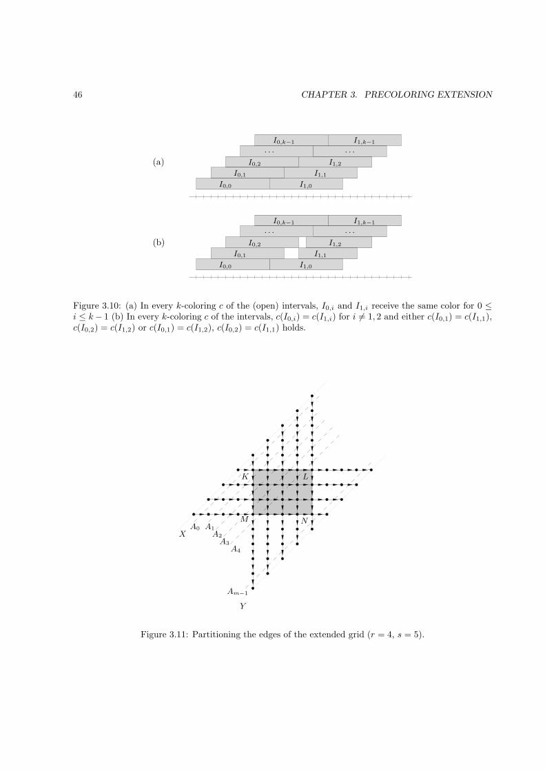
46 CHAPTER 3. PRECOLORING EXTENSION
(a)
(b)
I1,2
I1,2
I1,k−1
I1,k−1
I0,k−1
I0,k−1
I1,1
I1,1
. . . . . .
. . .. . .
I0,0
I0,0
I0,1
I0,1
I0,2
I0,2
I1,0
I1,0
Figure 3.10: (a) In every k-coloring c of the (open) intervals, I0,i and I1,i receive the same color for 0 ≤i ≤ k− 1 (b) In every k-coloring c of the intervals, c(I0,i) = c(I1,i) for i 6= 1, 2 and either c(I0,1) = c(I1,1),c(I0,2) = c(I1,2) or c(I0,1) = c(I1,2), c(I0,2) = c(I1,1) holds.
Am−1
A3A4
A2
A1A0
Y
X
NM
LK
Figure 3.11: Partitioning the edges of the extended grid (r = 4, s = 5).
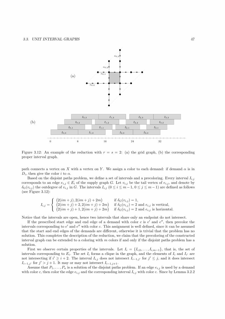
3.3. UNIT INTERVAL GRAPHS 47
(a)
e0,3
e0,2
e0,1
e0,0
(b)
32241680
I3,3
I3,2
I3,1
I3,0
I2,3
I2,2
I2,1
I2,0
I1,3
I1,2
I1,1
I1,0
I0,3
I0,2
I0,1
I0,0
Figure 3.12: An example of the reduction with r = s = 2: (a) the grid graph, (b) the correspondingproper interval graph.
path connects a vertex on X with a vertex on Y . We assign a color to each demand: if demand α is inDi, then give the color i to α.
Based on the disjoint paths problem, we define a set of intervals and a precoloring. Every interval Ii,jcorresponds to an edge ei,j ∈ Ei of the supply graph G. Let vi,j be the tail vertex of ei,j, and denote byδG(vi,j) the outdegree of vi,j in G. The intervals Ii,j (0 ≤ i ≤ m− 1, 0 ≤ j ≤ m− 1) are defined as follows(see Figure 3.12):
Ii,j =
(2(im+ j), 2(im+ j) + 2m
)if δG(vi,j) = 1,(
2(im+ j) + 2, 2(im+ j) + 2m)
if δG(vi,j) = 2 and ei,j is vertical,(2(im+ j) + 1, 2(im+ j) + 2m
)if δG(vi,j) = 2 and ei,j is horizontal.
Notice that the intervals are open, hence two intervals that share only an endpoint do not intersect.If the prescribed start edge and end edge of a demand with color c is e′ and e′′, then precolor the
intervals corresponding to e′ and e′′ with color c. This assignment is well defined, since it can be assumedthat the start and end edges of the demands are different, otherwise it is trivial that the problem has nosolution. This completes the description of the reduction, we claim that the precoloring of the constructedinterval graph can be extended to a coloring with m colors if and only if the disjoint paths problem has asolution.
First we observe certain properties of the intervals. Let Ii = {Ii,0, . . . , Ii,m−1}, that is, the set ofintervals corresponding to Ei. The set Ii forms a clique in the graph, and the elements of Ii and Ii′ arenot intersecting if i′ ≥ i + 2. The interval Ii,j does not intersect Ii−1,j′ for j′ ≤ j, and it does intersectIi−1,j′ for j′ > j + 1. It may or may not intersect Ii−1,j+1.
Assume that P1, . . . , Pn is a solution of the disjoint paths problem. If an edge ei,j is used by a demandwith color c, then color the edge ei,j and the corresponding interval Ii,j with color c. Since by Lemma 3.2.2
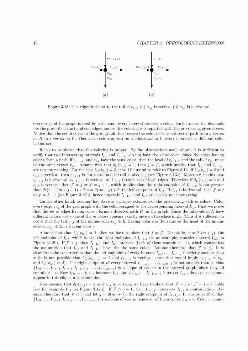
48 CHAPTER 3. PRECOLORING EXTENSION
ei,j−1
ei−1,j
ei−1,j−1 ei,jei,j+1ei−1,j
ei−1,j+1
ei,j
vi,j vi,j
(b)(a)
Figure 3.13: The edges incident to the tail of ei,j . (a) ei,j is vertical (b) ei,j is horizontal
every edge of the graph is used by a demand, every interval receives a color. Furthermore, the demandsuse the prescribed start and end edges, and so this coloring is compatible with the precoloring given above.Notice that the set of edges in the grid graph that receive the color c forms a directed path from a vertexon X to a vertex on Y . Thus all m colors appear on the intervals in Ii, every interval has different colorin this set.
It has to be shown that this coloring is proper. By the observations made above, it is sufficient toverify that two intersecting intervals Ii,j and Ii−1,j′ do not have the same color. Since the edges havingcolor c form a path, if ei−1,j′ and ei,j have the same color, then the head of ei−1,j′ and the tail of ei,j mustbe the same vertex vi,j . Assume first that δG(vi,j) = 1, then j = j′, which implies that Ii,j and Ii−1,j′
are not intersecting. For the case δG(vi,j) = 2, it will be useful to refer to Figure 3.13. If δG(vi,j) = 2 andei,j is vertical, then ei,j+1 is horizontal and its tail is also vi,j (see Figure 3.13a). Moreover, in this caseei−1,j is horizontal, ei−1,j+1 is vertical, and vi,j is the head of both edges. Therefore if δG(vi,j) = 2 andei,j is vertical, then j′ = j or j′ = j + 1, which implies that the right endpoint of Ii−1,j′ is not greaterthan 2((i− 1)m+ j + 1) + 2m = 2(im+ j) + 2, the left endpoint of Ii,j . If ei,j is horizontal, then j′ = jor j′ = j − 1 (see Figure 3.13b), hence intervals Ii−1,j′ and Ii,j are clearly not intersecting.
On the other hand, assume that there is a proper extension of the precoloring with m colors. Colorevery edge ei,j of the grid graph with the color assigned to the corresponding interval Ii,j . First we provethat the set of edges having color c forms a directed path Rc in the graph. Since the intervals in Ii havedifferent colors, every one of the m colors appears exactly once on the edges in Ei. Thus it is sufficient toprove that the tail vi,j of the unique edge ei,j ∈ Ei having color c is the same as the head of the uniqueedge ei−1,j′ ∈ Ei−1 having color c.
Assume first that δG(vi,j) = 1, then we have to show that j = j′. Denote by x = 2(im + j), theleft endpoint of Ii,j , which is also the right endpoint of Ii−1,j (as an example, consider interval I1,3 onFigure 3.12b). If j′ > j, then Ii−1,j′ and Ii,j intersect (both of them contain x + ǫ), which contradictsthe assumption that Ii,j and Ii−1,j′ have the the same color. Assume therefore that j′ < j. It isclear from the construction that the left endpoint of every interval Ii,1, . . . , Ii,j−1 is strictly smaller thanx (it is not possible that δG(vi,j−1) = 2 and ei,j−1 is vertical, since that would imply vi,j−1 = vi,jand δG(vi,j) = 2). The right endpoint of every interval Ii−1,j , . . . , Ii−1,m−1 is not smaller than x, thus{Ii,0, . . . , Ii,j−1, Ii−1,j , Ii−1,j+1, . . . , Ii−1,m−1} is a clique of size m in the interval graph, since they allcontain x− ǫ. Now Ii,0, . . . , Ii,j−1 intersect Ii,j , and Ii−1,j , . . . Ii−1,m−1 intersect Ii,j′ , thus color c cannotappear in this clique, a contradiction.
Now assume that δG(ei,j) = 2 and ei,j is vertical, we have to show that j′ = j or j′ = j + 1 holds(see for example I1,1 on Figure 3.12b). If j′ > j + 1, then Ii−1,j′ intersects Ii,j , a contradiction. As-sume therefore that j′ < j and let y = 2(im + j), the right endpoint of Ii−1,j . It can be verified that{Ii,0, . . . , Ii,j−1, Ii−1,j , . . . , Ii−1,m−1} is a clique of size m, since all of them contain y − ǫ. Color c cannot
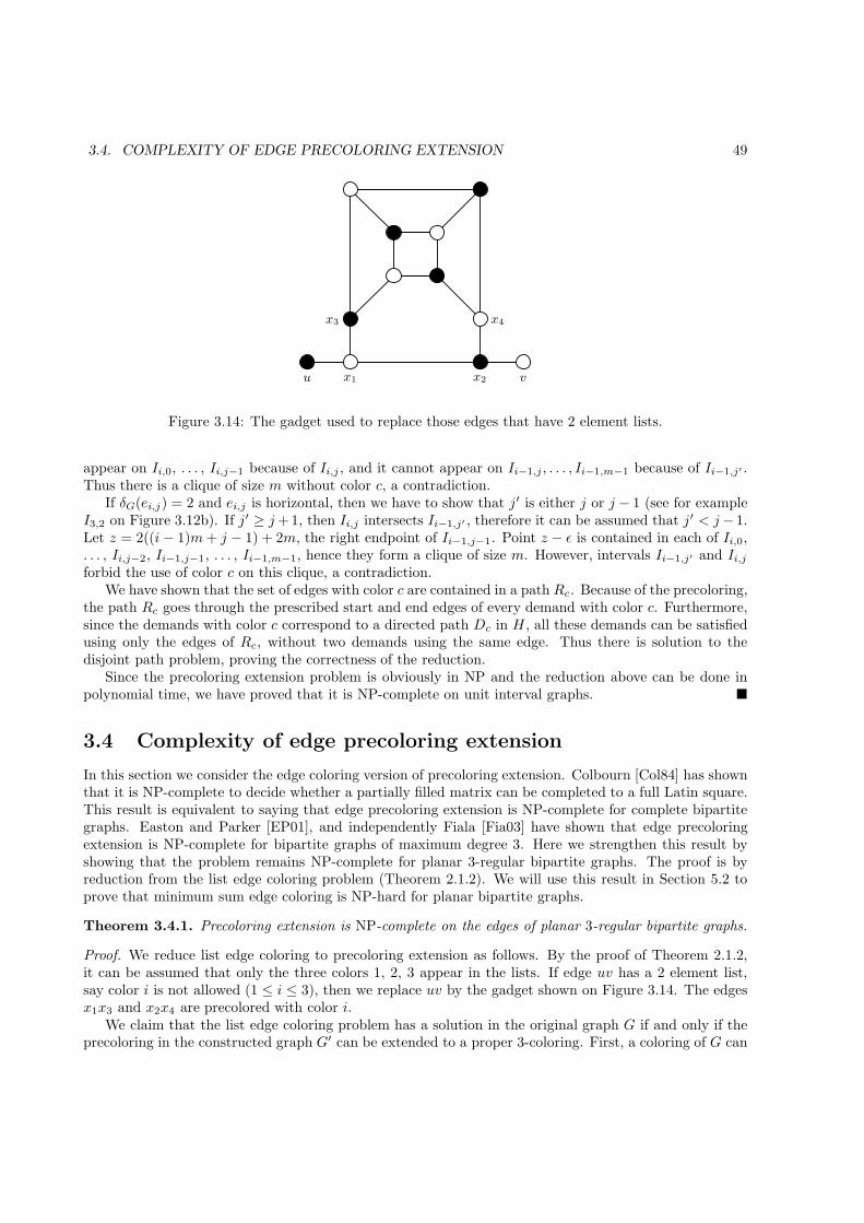
3.4. COMPLEXITY OF EDGE PRECOLORING EXTENSION 49
u x1 x2 v
x3 x4
Figure 3.14: The gadget used to replace those edges that have 2 element lists.
appear on Ii,0, . . . , Ii,j−1 because of Ii,j , and it cannot appear on Ii−1,j , . . . , Ii−1,m−1 because of Ii−1,j′ .Thus there is a clique of size m without color c, a contradiction.
If δG(ei,j) = 2 and ei,j is horizontal, then we have to show that j′ is either j or j − 1 (see for exampleI3,2 on Figure 3.12b). If j′ ≥ j+ 1, then Ii,j intersects Ii−1,j′ , therefore it can be assumed that j′ < j− 1.Let z = 2((i− 1)m+ j − 1) + 2m, the right endpoint of Ii−1,j−1. Point z − ǫ is contained in each of Ii,0,. . . , Ii,j−2, Ii−1,j−1, . . . , Ii−1,m−1, hence they form a clique of size m. However, intervals Ii−1,j′ and Ii,jforbid the use of color c on this clique, a contradiction.
We have shown that the set of edges with color c are contained in a path Rc. Because of the precoloring,the path Rc goes through the prescribed start and end edges of every demand with color c. Furthermore,since the demands with color c correspond to a directed path Dc in H , all these demands can be satisfiedusing only the edges of Rc, without two demands using the same edge. Thus there is solution to thedisjoint path problem, proving the correctness of the reduction.
Since the precoloring extension problem is obviously in NP and the reduction above can be done inpolynomial time, we have proved that it is NP-complete on unit interval graphs. �
3.4 Complexity of edge precoloring extension
In this section we consider the edge coloring version of precoloring extension. Colbourn [Col84] has shownthat it is NP-complete to decide whether a partially filled matrix can be completed to a full Latin square.This result is equivalent to saying that edge precoloring extension is NP-complete for complete bipartitegraphs. Easton and Parker [EP01], and independently Fiala [Fia03] have shown that edge precoloringextension is NP-complete for bipartite graphs of maximum degree 3. Here we strengthen this result byshowing that the problem remains NP-complete for planar 3-regular bipartite graphs. The proof is byreduction from the list edge coloring problem (Theorem 2.1.2). We will use this result in Section 5.2 toprove that minimum sum edge coloring is NP-hard for planar bipartite graphs.
Theorem 3.4.1. Precoloring extension is NP-complete on the edges of planar 3-regular bipartite graphs.
Proof. We reduce list edge coloring to precoloring extension as follows. By the proof of Theorem 2.1.2,it can be assumed that only the three colors 1, 2, 3 appear in the lists. If edge uv has a 2 element list,say color i is not allowed (1 ≤ i ≤ 3), then we replace uv by the gadget shown on Figure 3.14. The edgesx1x3 and x2x4 are precolored with color i.
We claim that the list edge coloring problem has a solution in the original graph G if and only if theprecoloring in the constructed graph G′ can be extended to a proper 3-coloring. First, a coloring of G can
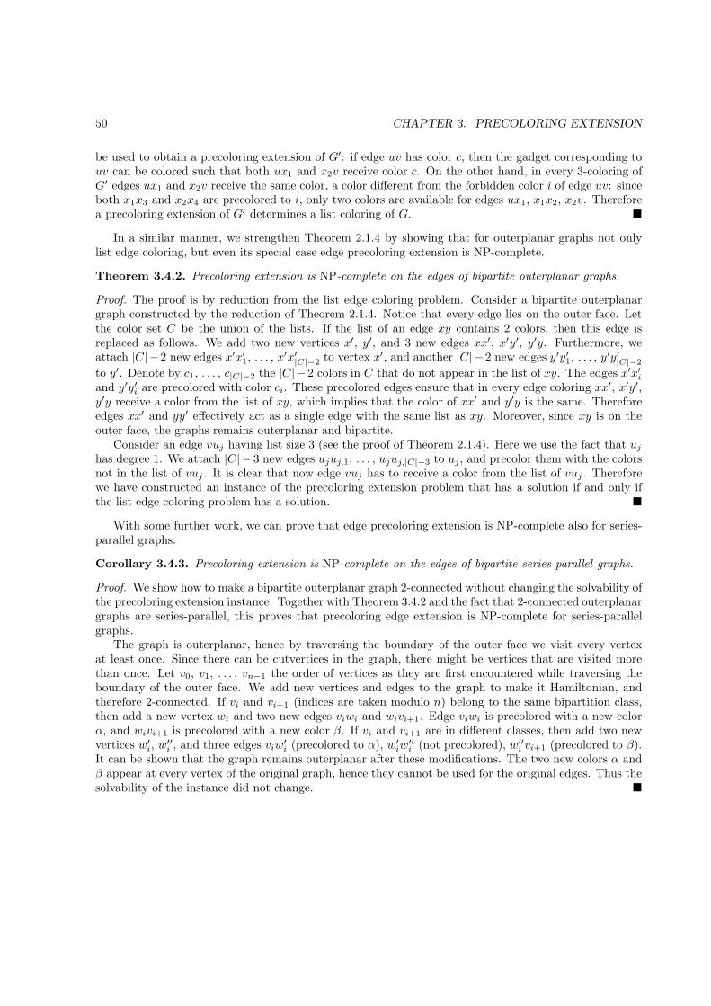
50 CHAPTER 3. PRECOLORING EXTENSION
be used to obtain a precoloring extension of G′: if edge uv has color c, then the gadget corresponding touv can be colored such that both ux1 and x2v receive color c. On the other hand, in every 3-coloring ofG′ edges ux1 and x2v receive the same color, a color different from the forbidden color i of edge uv: sinceboth x1x3 and x2x4 are precolored to i, only two colors are available for edges ux1, x1x2, x2v. Thereforea precoloring extension of G′ determines a list coloring of G. �
In a similar manner, we strengthen Theorem 2.1.4 by showing that for outerplanar graphs not onlylist edge coloring, but even its special case edge precoloring extension is NP-complete.
Theorem 3.4.2. Precoloring extension is NP-complete on the edges of bipartite outerplanar graphs.
Proof. The proof is by reduction from the list edge coloring problem. Consider a bipartite outerplanargraph constructed by the reduction of Theorem 2.1.4. Notice that every edge lies on the outer face. Letthe color set C be the union of the lists. If the list of an edge xy contains 2 colors, then this edge isreplaced as follows. We add two new vertices x′, y′, and 3 new edges xx′, x′y′, y′y. Furthermore, weattach |C|−2 new edges x′x′1, . . . , x′x′|C|−2 to vertex x′, and another |C|−2 new edges y′y′1, . . . , y′y′|C|−2
to y′. Denote by c1, . . . , c|C|−2 the |C|−2 colors in C that do not appear in the list of xy. The edges x′x′iand y′y′i are precolored with color ci. These precolored edges ensure that in every edge coloring xx′, x′y′,y′y receive a color from the list of xy, which implies that the color of xx′ and y′y is the same. Thereforeedges xx′ and yy′ effectively act as a single edge with the same list as xy. Moreover, since xy is on theouter face, the graphs remains outerplanar and bipartite.
Consider an edge vuj having list size 3 (see the proof of Theorem 2.1.4). Here we use the fact that ujhas degree 1. We attach |C| − 3 new edges ujuj,1, . . . , ujuj,|C|−3 to uj, and precolor them with the colorsnot in the list of vuj . It is clear that now edge vuj has to receive a color from the list of vuj . Thereforewe have constructed an instance of the precoloring extension problem that has a solution if and only ifthe list edge coloring problem has a solution. �
With some further work, we can prove that edge precoloring extension is NP-complete also for series-parallel graphs:
Corollary 3.4.3. Precoloring extension is NP-complete on the edges of bipartite series-parallel graphs.
Proof. We show how to make a bipartite outerplanar graph 2-connected without changing the solvability ofthe precoloring extension instance. Together with Theorem 3.4.2 and the fact that 2-connected outerplanargraphs are series-parallel, this proves that precoloring edge extension is NP-complete for series-parallelgraphs.
The graph is outerplanar, hence by traversing the boundary of the outer face we visit every vertexat least once. Since there can be cutvertices in the graph, there might be vertices that are visited morethan once. Let v0, v1, . . . , vn−1 the order of vertices as they are first encountered while traversing theboundary of the outer face. We add new vertices and edges to the graph to make it Hamiltonian, andtherefore 2-connected. If vi and vi+1 (indices are taken modulo n) belong to the same bipartition class,then add a new vertex wi and two new edges viwi and wivi+1. Edge viwi is precolored with a new colorα, and wivi+1 is precolored with a new color β. If vi and vi+1 are in different classes, then add two newvertices w′
i, w′′i , and three edges viw
′i (precolored to α), w′
iw′′i (not precolored), w′′
i vi+1 (precolored to β).It can be shown that the graph remains outerplanar after these modifications. The two new colors α andβ appear at every vertex of the original graph, hence they cannot be used for the original edges. Thus thesolvability of the instance did not change. �
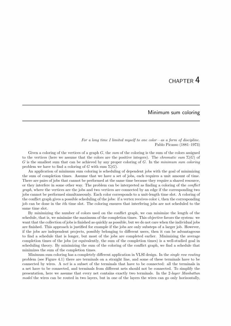
CHAPTER 4
Minimum sum coloring
For a long time I limited myself to one color—as a form of discipline.Pablo Picasso (1881–1973)
Given a coloring of the vertices of a graph G, the sum of the coloring is the sum of the colors assignedto the vertices (here we assume that the colors are the positive integers). The chromatic sum Σ(G) ofG is the smallest sum that can be achieved by any proper coloring of G. In the minimum sum coloringproblem we have to find a coloring of G with sum Σ(G).
An application of minimum sum coloring is scheduling of dependent jobs with the goal of minimizingthe sum of completion times. Assume that we have a set of jobs, each requires a unit amount of time.There are pairs of jobs that cannot be performed at the same time because they require a shared resource,or they interfere in some other way. The problem can be interpreted as finding a coloring of the conflictgraph, where the vertices are the jobs and two vertices are connected by an edge if the corresponding twojobs cannot be performed simultaneously. Each color corresponds to a unit-length time slot. A coloring ofthe conflict graph gives a possible scheduling of the jobs: if a vertex receives color i, then the correspondingjob can be done in the ith time slot. The coloring ensures that interfering jobs are not scheduled to thesame time slot.
By minimizing the number of colors used on the conflict graph, we can minimize the length of theschedule, that is, we minimize the maximum of the completion times. This objective favors the system: wewant that the collection of jobs is finished as quickly as possible, but we do not care when the individual jobsare finished. This approach is justified for example if the jobs are only substeps of a larger job. However,if the jobs are independent projects, possibly belonging to different users, then it can be advantageousto find a schedule that is longer, but most of the jobs are completed earlier. Minimizing the averagecompletion times of the jobs (or equivalently, the sum of the completion times) is a well-studied goal inscheduling theory. By minimizing the sum of the coloring of the conflict graph, we find a schedule thatminimizes the sum of the completion times.
Minimum sum coloring has a completely different application in VLSI design. In the single row routingproblem (see Figure 4.1) there are terminals on a straight line, and some of these terminals have to beconnected by wires. A net is a subset of the terminals that have to be connected: all the terminals ina net have to be connected, and terminals from different nets should not be connected. To simplify thepresentation, here we assume that every net contains exactly two terminals. In the 2-layer Manhattanmodel the wires can be routed in two layers, but in one of the layers the wires can go only horizontally,
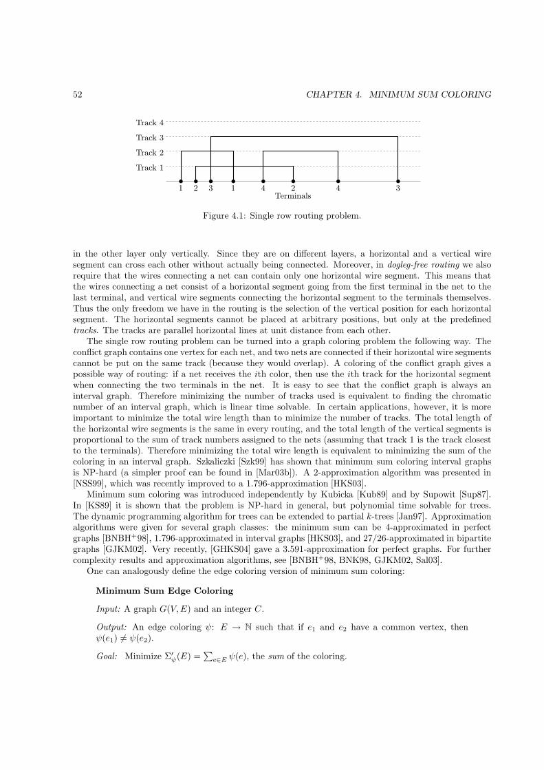
52 CHAPTER 4. MINIMUM SUM COLORING
PSfrag
11 22 44 33
Track 4
Track 1
Track 2
Track 3
Terminals
Figure 4.1: Single row routing problem.
in the other layer only vertically. Since they are on different layers, a horizontal and a vertical wiresegment can cross each other without actually being connected. Moreover, in dogleg-free routing we alsorequire that the wires connecting a net can contain only one horizontal wire segment. This means thatthe wires connecting a net consist of a horizontal segment going from the first terminal in the net to thelast terminal, and vertical wire segments connecting the horizontal segment to the terminals themselves.Thus the only freedom we have in the routing is the selection of the vertical position for each horizontalsegment. The horizontal segments cannot be placed at arbitrary positions, but only at the predefinedtracks. The tracks are parallel horizontal lines at unit distance from each other.
The single row routing problem can be turned into a graph coloring problem the following way. Theconflict graph contains one vertex for each net, and two nets are connected if their horizontal wire segmentscannot be put on the same track (because they would overlap). A coloring of the conflict graph gives apossible way of routing: if a net receives the ith color, then use the ith track for the horizontal segmentwhen connecting the two terminals in the net. It is easy to see that the conflict graph is always aninterval graph. Therefore minimizing the number of tracks used is equivalent to finding the chromaticnumber of an interval graph, which is linear time solvable. In certain applications, however, it is moreimportant to minimize the total wire length than to minimize the number of tracks. The total length ofthe horizontal wire segments is the same in every routing, and the total length of the vertical segments isproportional to the sum of track numbers assigned to the nets (assuming that track 1 is the track closestto the terminals). Therefore minimizing the total wire length is equivalent to minimizing the sum of thecoloring in an interval graph. Szkaliczki [Szk99] has shown that minimum sum coloring interval graphsis NP-hard (a simpler proof can be found in [Mar03b]). A 2-approximation algorithm was presented in[NSS99], which was recently improved to a 1.796-approximation [HKS03].
Minimum sum coloring was introduced independently by Kubicka [Kub89] and by Supowit [Sup87].In [KS89] it is shown that the problem is NP-hard in general, but polynomial time solvable for trees.The dynamic programming algorithm for trees can be extended to partial k-trees [Jan97]. Approximationalgorithms were given for several graph classes: the minimum sum can be 4-approximated in perfectgraphs [BNBH+98], 1.796-approximated in interval graphs [HKS03], and 27/26-approximated in bipartitegraphs [GJKM02]. Very recently, [GHKS04] gave a 3.591-approximation for perfect graphs. For furthercomplexity results and approximation algorithms, see [BNBH+98, BNK98, GJKM02, Sal03].
One can analogously define the edge coloring version of minimum sum coloring:
Minimum Sum Edge Coloring
Input: A graph G(V,E) and an integer C.
Output: An edge coloring ψ: E → N such that if e1 and e2 have a common vertex, thenψ(e1) 6= ψ(e2).
Goal: Minimize Σ′ψ(E) =
∑e∈E ψ(e), the sum of the coloring.
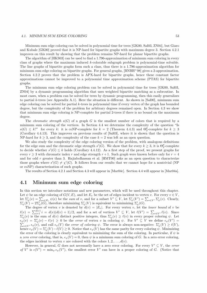
4.1. MINIMUM SUM EDGE COLORING 53
Minimum sum edge coloring can be solved in polynomial time for trees [GK00, Sal03, ZN04], but Giaroand Kubale [GK00] proved that it is NP-hard for bipartite graphs with maximum degree 3. Section 4.2.1improves on this result by showing that the problem remains NP-hard for planar bipartite graphs.
The algorithm of [HKS03] can be used to find a 1.796-approximation of minimum sum coloring in everyclass of graphs where the maximum induced k-colorable subgraph problem is polynomial-time solvable.The line graphs of bipartite graphs form such a class, thus there is a 1.796-approximation algorithm forminimum sum edge coloring on bipartite graphs. For general graphs, [BNBH+98] gives a 2-approximation.Section 4.2.2 proves that the problem is APX-hard for bipartite graphs, hence these constant factorapproximations cannot be improved to a polynomial time approximation scheme (PTAS) for bipartitegraphs.
The minimum sum edge coloring problem can be solved in polynomial time for trees [GK00, Sal03,ZN04] by a dynamic programming algorithm that uses weighted bipartite matching as a subroutine. Inmost cases, when a problem can be solved for trees by dynamic programming, then this easily generalizesto partial k-trees (see Appendix A.1). Here the situation is different. As shown in [Sal00], minimum sumedge coloring can be solved for partial k-trees in polynomial time if every vertex of the graph has boundeddegree, but the complexity of the problem for arbitrary degrees remained open. In Section 4.3 we showthat minimum sum edge coloring is NP-complete for partial 2-trees if there is no bound on the maximumdegree.
The chromatic strength s(G) of a graph G is the smallest number of colors that is required by aminimum sum coloring of the vertices. In Section 4.4 we determine the complexity of the question “Iss(G) ≤ k?” for every k: it is coNP-complete for k = 2 (Theorem 4.4.3) and Θp
2-complete for k ≥ 3(Corollary 4.4.13). This improves on previous results of [Sal03], where it is shown that the question isNP-hard for k ≥ 3, and the complexity of the case k = 2 was left as an open question.
We also study the complexity of the edge coloring version of the problem, with analogous definitionsfor the edge sum and the chromatic edge strength s′(G). We show that for every k ≥ 3, it is Θp
2-completeto decide whether s′(G) ≤ k holds (Corollary 4.4.12). As a first step of the proof, we present graphs forevery r ≥ 3 with chromatic index r and edge strength r+ 1. Such graph were known before only for r = 4and for odd r greater than 3. Hajiabolhassan et al. [HMT00] asks as an open question to characterizethose graphs where s′(G) 6= χ′(G). It follows from our results that we cannot hope for a nontrivial (NPor coNP) characterization of such graphs.
The results of Section 4.2.1 and Section 4.3 will appear in [Mar04c]. Section 4.4 will appear in [Mar04a].
4.1 Minimum sum edge coloring
In this section we introduce notations and new parameters, which will be used throughout this chapter.Let ψ be an edge coloring of G(V,E), and let Ev be the set of edges incident to vertex v. For every v ∈ V ,let Σ′
ψ(v) =∑
e∈Evψ(e) be the sum of v, and for a subset V ′ ⊆ V , let Σ′
ψ(V ′) =∑v∈V ′ Σ′
ψ(v). Clearly,Σ′ψ(V ) = 2Σ′
ψ(G), therefore minimizing Σ′ψ(V ) is equivalent to minimizing Σ′
ψ(G).The degree of vertex v is denoted by d(v) = |Ev|. For every vertex v, let the lower bound of v be
ℓ(v) =∑d(v)i=1 i = d(v)(d(v) + 1)/2, and for a set of vertices V ′ ⊆ V , let ℓ(V ′) =
∑v∈V ′ ℓ(v). Since
Σ′ψ(v) is the sum of d(v) distinct positive integers, thus Σ′
ψ(v) ≥ ℓ(v) in every proper coloring ψ. Letǫψ(v) = Σ′
ψ(v) − ℓ(v) ≥ 0 be the error of vertex v in coloring ψ. For V ′ ⊆ V we define ǫψ(V ′) =∑v∈V ′ ǫψ(v), and call ǫψ(V ) the error of coloring ψ. The error is always non-negative: Σ′
ψ(V ) ≥ ℓ(V ),hence ǫψ(V ) = Σ′
ψ(V )−ℓ(V ) ≥ 0. Notice that ǫψ(V ) has the same parity for every coloring ψ. Minimizingthe error of the coloring is clearly equivalent to minimizing the sum of the coloring. In particular, if ψ isa zero error coloring, that is, ǫψ(V ) = 0, then ψ is a minimum sum coloring of G. In a zero error coloring,the edges incident to vertex v are colored with the colors 1, 2, . . . , d(v).
However, in general, G does not necessarily have a zero error coloring. For every V ′ ⊆ V , the errorof V ′ is ǫ(V ′) = minψ ǫψ(V ′), the smallest error V ′ can have in a proper coloring of G. (Notice that

54 CHAPTER 4. MINIMUM SUM COLORING
ǫ(V ′) =∑
v∈V ′ ǫ({v}) does not always hold, in fact, ǫ({v}) = 0 for every v ∈ V ). Deciding whether Ghas a zero error coloring is a special case of the minimum sum edge coloring problem. It might be worthpointing out that finding a zero error coloring is very different from finding a minimum sum coloring: zeroerror is a local constraint on the coloring (every vertex has to have zero error), while minimizing the sumis a global constraint. In Section 4.2, when we prove the NP-completeness of minimum sum edge coloringfor planar bipartite graphs, we will utilize this connection to reduce a local problem, edge precoloringextension, to the global problem of minimizing the sum.
Quasigraphs. Parallel edges are not allowed for the graphs considered here. However, for conveniencewe extend the problem by introducing half-loops. Following [Lov97], a half-loop is a loop that contributesonly 1 to the degree of its end vertex. Every vertex has at most one half-loop. If a graph is allowed tohave at most one half-loop at every vertex, then it will be called a quasigraph. In a quasigraph, the sumof an edge coloring is defined to be the sum of the color of the edges plus half the sum of the color of thehalf-loops, therefore the sum of a quasigraph is not necessarily integer. However, the error of a coloring isalways integer, and with these definitions it remains true that the sum of the vertices is twice the sum ofthe edges. A quasigraph will be called bipartite if removing the half-loops gives a bipartite graph.
The following observation shows that allowing half-loops does not make determining the minimumedge sum or the chromatic edge strength more difficult:
Proposition 4.1.1. Given a quasigraph G, one can create in polynomial time a graph G′ such thatΣ′(G′) = 2Σ′(G) and s′(G′) = s′(G).
Proof. To obtain G′, take two disjoint copies G1, G2 of G and remove every half-loop. If there was ahalf-loop at v in G, then add an edge v1v2 to G′, where v1 and v2 are the vertices corresponding to v inG1 and G2, respectively. In graph G′, to every edge give the color of the corresponding edge in G. If thesum of the coloring in G was S, then we obtain a coloring in G′ with sum 2S: two edges of G′ correspondto every edge of G, but only one edge corresponds to every half-loop of G.
On the other hand, one can show that if G′ has a k-coloring with sum S, than G has a k-coloring withsum at most S/2. The edges of G′ can be partitioned into three sets E1, E2, E
′: set Ei contains the edgesinduced by Gi (i = 1, 2), and E′ contains the edges corresponding to the half-loops. It can be assumedthat every edge in E1 has the same color as its counterpart in E2: otherwise if the sum of the edges in,say, E1 is not greater than the sum of the edges in E2, then recoloring every edge in E2 with the color ofits pair in E1 results in a proper coloring without increasing the sum. Now color every edge of G with thecolor of its two corresponding edges in G′, and color every half-loop with the color of its correspondingedge in G′. The sum of this coloring is exactly half the sum of the coloring of G′. �
Therefore finding a minimum sum edge coloring on the quasigraph G is the same problem as findinga minimum sum edge coloring on the corresponding graph G′. In particular, the edge strength of G andG′ are the same. In Section 4.4.4, we show that it is Θp
2-complete to determine the edge strength of aquasigraph. By the above construction, Θp
2-completeness follows for ordinary simple graphs as well.Notice that if G is bipartite, then G′ is bipartite as well. On the other hand, the transformation does
not preserve planarity in general.
Gadgets. The reductions in this chapter are of the component design type: we build “gadgets” cor-responding to vertices and edges, and in the reduction a larger graph is constructed from these smallergraphs. In some cases, these gadgets themselves are also built from smaller gadgets. Here we introducethe terminology and the notational conventions that will be used while working with gadgets.
A gadget is a graph whose vertices are divided into external and internal vertices. On the figures,the external vertices of the gadgets are framed (see for example Figure 4.5 or Figure 4.6). If an externalvertex has degree one, then the edge incident to it will be called a pendant edge (for example, the gadgeton Figure 4.5 has 3 pendant edges).
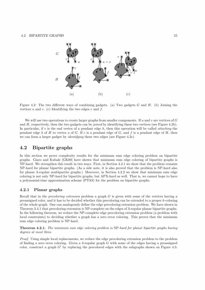
4.2. BIPARTITE GRAPHS 55
v
u = v
(b)(a) (c)
v
u
uf
f
G
H
e e
e = f
Figure 4.2: The two different ways of combining gadgets. (a) Two gadgets G and H . (b) Joining thevertices u and v. (c) Identifying the two edges e and f .
We will use two operations to create larger graphs from smaller components. If u and v are vertices of Gand H , respectively, then the two gadgets can be joined by identifying these two vertices (see Figure 4.2b).In particular, if v is the end vertex of a pendant edge h, then this operation will be called attaching thependant edge h of H to vertex u of G. If e is a pendant edge of G, and f is a pendant edge of H , thenwe can form a larger gadget by identifying these two edges (see Figure 4.2c).
4.2 Bipartite graphs
In this section we prove complexity results for the minimum sum edge coloring problem on bipartitegraphs. Giaro and Kubale [GK00] have shown that minimum sum edge coloring of bipartite graphs isNP-hard. We strengthen this result in two ways. First, in Section 4.2.1 we show that the problem remainsNP-hard for planar bipartite graphs. (As a side note, it is also proved that the problem is NP-hard alsofor planar 3-regular nonbipartite graphs.) Moreover, in Section 4.2.2 we show that minimum sum edgecoloring is not only NP-hard for bipartite graphs, but APX-hard as well. That is, we cannot hope to havea polynomial-time approximation scheme (PTAS) for the problem on bipartite graphs.
4.2.1 Planar graphs
Recall that in the precoloring extension problem a graph G is given with some of the vertices having apreassigned color, and it has to be decided whether this precoloring can be extended to a proper k-coloringof the whole graph. One can analogously define the edge precoloring extension problem. We have shown inTheorem 3.4.1 that precoloring extension is NP-complete on the edges of 3-regular planar bipartite graphs.In the following theorem, we reduce the NP-complete edge precoloring extension problem (a problem withlocal constraints) to deciding whether a graph has a zero error coloring. This proves that the minimumsum edge coloring problem is NP-hard.
Theorem 4.2.1. The minimum sum edge coloring problem is NP-hard for planar bipartite graphs havingdegrees at most three.
Proof. Using simple local replacements, we reduce the edge precoloring extension problem to the problemof finding a zero error coloring. Given a 3-regular graph G with some of the edges having a preassignedcolor, construct a graph G′ by replacing the precolored edges with the subgraphs shown on Figure 4.3.
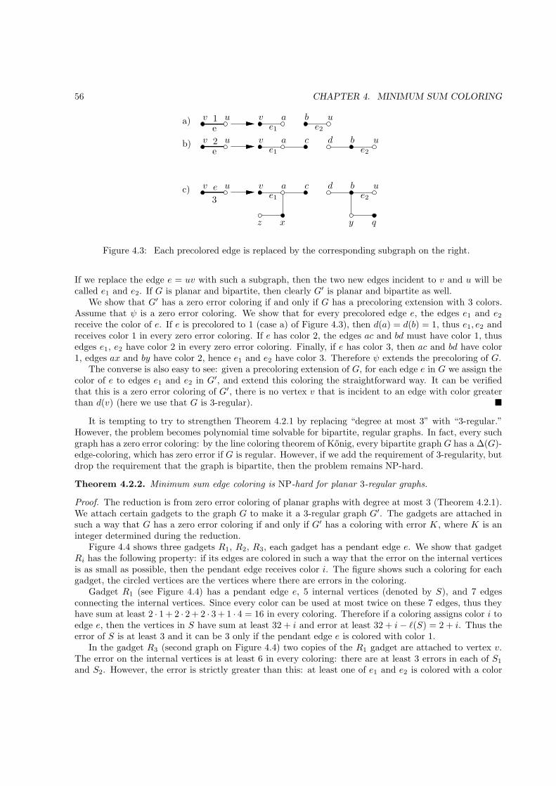
56 CHAPTER 4. MINIMUM SUM COLORING
e
e2
e2
e2
a)
b)
c)3
a
a
a
c
c
b
b
b2
1e
e
d
d
u
u
u
u
u
u
v
v
vv
v
ve1
e1
e1
y qxz
Figure 4.3: Each precolored edge is replaced by the corresponding subgraph on the right.
If we replace the edge e = uv with such a subgraph, then the two new edges incident to v and u will becalled e1 and e2. If G is planar and bipartite, then clearly G′ is planar and bipartite as well.
We show that G′ has a zero error coloring if and only if G has a precoloring extension with 3 colors.Assume that ψ is a zero error coloring. We show that for every precolored edge e, the edges e1 and e2receive the color of e. If e is precolored to 1 (case a) of Figure 4.3), then d(a) = d(b) = 1, thus e1, e2 andreceives color 1 in every zero error coloring. If e has color 2, the edges ac and bd must have color 1, thusedges e1, e2 have color 2 in every zero error coloring. Finally, if e has color 3, then ac and bd have color1, edges ax and by have color 2, hence e1 and e2 have color 3. Therefore ψ extends the precoloring of G.
The converse is also easy to see: given a precoloring extension of G, for each edge e in G we assign thecolor of e to edges e1 and e2 in G′, and extend this coloring the straightforward way. It can be verifiedthat this is a zero error coloring of G′, there is no vertex v that is incident to an edge with color greaterthan d(v) (here we use that G is 3-regular). �
It is tempting to try to strengthen Theorem 4.2.1 by replacing “degree at most 3” with “3-regular.”However, the problem becomes polynomial time solvable for bipartite, regular graphs. In fact, every suchgraph has a zero error coloring: by the line coloring theorem of Konig, every bipartite graph G has a ∆(G)-edge-coloring, which has zero error if G is regular. However, if we add the requirement of 3-regularity, butdrop the requirement that the graph is bipartite, then the problem remains NP-hard.
Theorem 4.2.2. Minimum sum edge coloring is NP-hard for planar 3-regular graphs.
Proof. The reduction is from zero error coloring of planar graphs with degree at most 3 (Theorem 4.2.1).We attach certain gadgets to the graph G to make it a 3-regular graph G′. The gadgets are attached insuch a way that G has a zero error coloring if and only if G′ has a coloring with error K, where K is aninteger determined during the reduction.
Figure 4.4 shows three gadgets R1, R2, R3, each gadget has a pendant edge e. We show that gadgetRi has the following property: if its edges are colored in such a way that the error on the internal verticesis as small as possible, then the pendant edge receives color i. The figure shows such a coloring for eachgadget, the circled vertices are the vertices where there are errors in the coloring.
Gadget R1 (see Figure 4.4) has a pendant edge e, 5 internal vertices (denoted by S), and 7 edgesconnecting the internal vertices. Since every color can be used at most twice on these 7 edges, thus theyhave sum at least 2 · 1 + 2 · 2 + 2 · 3 + 1 · 4 = 16 in every coloring. Therefore if a coloring assigns color i toedge e, then the vertices in S have sum at least 32 + i and error at least 32 + i− ℓ(S) = 2 + i. Thus theerror of S is at least 3 and it can be 3 only if the pendant edge e is colored with color 1.
In the gadget R3 (second graph on Figure 4.4) two copies of the R1 gadget are attached to vertex v.The error on the internal vertices is at least 6 in every coloring: there are at least 3 errors in each of S1
and S2. However, the error is strictly greater than this: at least one of e1 and e2 is colored with a color
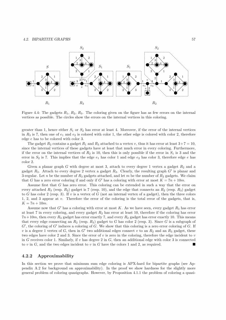
4.2. BIPARTITE GRAPHS 57
R3R1
v
R2
3
22 2
3
3
3
3
3 22 2
11 1
11 1 12
2
2
11
22
2
2
2
2 1
1
1
33
1 11 1
4 4
4
4
4
43 3
3
3
3
3
eve3
e2
e1 e1e e
S2 S2
S1 S1S
Figure 4.4: The gadgets R1, R2, R3. The coloring given on the figure has as few errors on the internalvertices as possible. The circles show the errors on the internal vertices in this coloring.
greater than 1, hence either S1 or S2 has error at least 4. Moreover, if the error of the internal verticesin R3 is 7, then one of e1 and e2 is colored with color 1, the other edge is colored with color 2, thereforeedge e has to be colored with color 3.
The gadget R2 contains a gadget R1 and R3 attached to a vertex v, thus it has error at least 3+7 = 10,since the internal vertices of these gadgets have at least that much error in every coloring. Furthermore,if the error on the internal vertices of R2 is 10, then this is only possible if the error in S1 is 3 and theerror in S2 is 7. This implies that the edge e1 has color 1 and edge e2 has color 3, therefore edge e hascolor 2.
Given a planar graph G with degree at most 3, attach to every degree 1 vertex a gadget R2 and agadget R3. Attach to every degree 2 vertex a gadget R3. Clearly, the resulting graph G′ is planar and3-regular. Let n be the number of R3 gadgets attached, and let m be the number of R2 gadgets. We claimthat G has a zero error coloring if and only if G′ has a coloring with error at most K = 7n+ 10m.
Assume first that G has zero error. This coloring can be extended in such a way that the error onevery attached R3 (resp. R2) gadget is 7 (resp. 10), and the edge that connects an R2 (resp. R3) gadgetto G has color 2 (resp. 3). If v is a vertex of G (not an internal vertex of a gadget), then the three colors1, 2, and 3 appear at v. Therefore the error of the coloring is the total error of the gadgets, that is,K = 7n+ 10m.
Assume now that G′ has a coloring with error at most K. As we have seen, every gadget R3 has errorat least 7 in every coloring, and every gadget R2 has error at least 10, therefore if the coloring has error7n+10m, then every R3 gadget has error exactly 7, and every R2 gadget has error exactly 10. This meansthat every edge connecting an R2 (resp. R3) gadget to G has color 2 (resp. 3). Since G is a subgraph ofG′, the coloring of G′ induces a coloring of G. We show that this coloring is a zero error coloring of G. Ifv is a degree 1 vertex of G, then in G′ two additional edges connect v to an R2 and an R3 gadget, thesetwo edges have color 2 and 3. Since the error of v is zero in the coloring, therefore the edge incident to vin G receives color 1. Similarly, if v has degree 2 in G, then an additional edge with color 3 is connectedto v in G, and the two edges incident to v in G have the colors 1 and 2, as required. �
4.2.2 Approximability
In this section we prove that minimum sum edge coloring is APX-hard for bipartite graphs (see Ap-pendix A.2 for background on approximability). In the proof we show hardness for the slightly moregeneral problem of coloring quasigraphs. However, by Proposition 4.1.1 the problem of coloring a quasi-
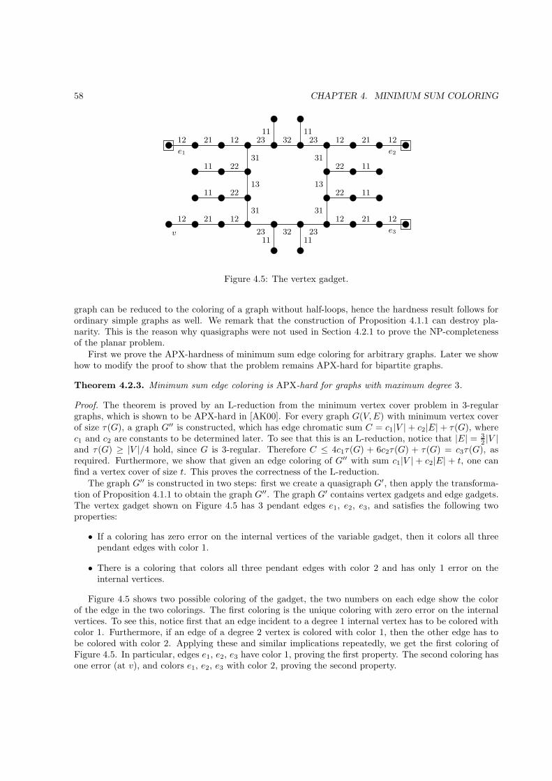
58 CHAPTER 4. MINIMUM SUM COLORING
e3
e2e1
v
3223 23
3223 23
13
31
31
13
31
31
22
2222
2211
11 11
11
11
11
11
11
21
21
21
21
12 12
12 12
12 12
1212
Figure 4.5: The vertex gadget.
graph can be reduced to the coloring of a graph without half-loops, hence the hardness result follows forordinary simple graphs as well. We remark that the construction of Proposition 4.1.1 can destroy pla-narity. This is the reason why quasigraphs were not used in Section 4.2.1 to prove the NP-completenessof the planar problem.
First we prove the APX-hardness of minimum sum edge coloring for arbitrary graphs. Later we showhow to modify the proof to show that the problem remains APX-hard for bipartite graphs.
Theorem 4.2.3. Minimum sum edge coloring is APX-hard for graphs with maximum degree 3.
Proof. The theorem is proved by an L-reduction from the minimum vertex cover problem in 3-regulargraphs, which is shown to be APX-hard in [AK00]. For every graph G(V,E) with minimum vertex coverof size τ(G), a graph G′′ is constructed, which has edge chromatic sum C = c1|V | + c2|E| + τ(G), wherec1 and c2 are constants to be determined later. To see that this is an L-reduction, notice that |E| = 3
2 |V |and τ(G) ≥ |V |/4 hold, since G is 3-regular. Therefore C ≤ 4c1τ(G) + 6c2τ(G) + τ(G) = c3τ(G), asrequired. Furthermore, we show that given an edge coloring of G′′ with sum c1|V | + c2|E| + t, one canfind a vertex cover of size t. This proves the correctness of the L-reduction.
The graph G′′ is constructed in two steps: first we create a quasigraph G′, then apply the transforma-tion of Proposition 4.1.1 to obtain the graph G′′. The graph G′ contains vertex gadgets and edge gadgets.The vertex gadget shown on Figure 4.5 has 3 pendant edges e1, e2, e3, and satisfies the following twoproperties:
• If a coloring has zero error on the internal vertices of the variable gadget, then it colors all threependant edges with color 1.
• There is a coloring that colors all three pendant edges with color 2 and has only 1 error on theinternal vertices.
Figure 4.5 shows two possible coloring of the gadget, the two numbers on each edge show the colorof the edge in the two colorings. The first coloring is the unique coloring with zero error on the internalvertices. To see this, notice first that an edge incident to a degree 1 internal vertex has to be colored withcolor 1. Furthermore, if an edge of a degree 2 vertex is colored with color 1, then the other edge has tobe colored with color 2. Applying these and similar implications repeatedly, we get the first coloring ofFigure 4.5. In particular, edges e1, e2, e3 have color 1, proving the first property. The second coloring hasone error (at v), and colors e1, e2, e3 with color 2, proving the second property.
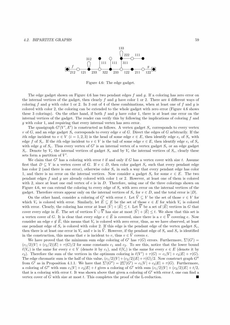
4.2. BIPARTITE GRAPHS 59
133
111
311111 111312
211322233 233121212 122 122
gf
222
Figure 4.6: The edge gadget.
The edge gadget shown on Figure 4.6 has two pendant edges f and g. If a coloring has zero error onthe internal vertices of the gadget, then clearly f and g have color 1 or 2. There are 4 different ways ofcoloring f and g with color 1 or 2. In 3 out of 4 of these combinations, when at least one of f and g iscolored with color 2, the coloring can be extended to the whole gadget with zero error (Figure 4.6 showsthese 3 colorings). On the other hand, if both f and g have color 1, there is at least one error on theinternal vertices of the gadget. The reader can verify this by following the implications of coloring f andg with color 1, and requiring that every internal vertex has zero error.
The quasigraph G′(V ′, E′) is constructed as follows. A vertex gadget Sv corresponds to every vertexv of G, and an edge gadget Se corresponds to every edge e of G. Direct the edges of G arbitrarily. If theith edge incident to v ∈ V (i = 1, 2, 3) is the head of some edge e ∈ E, then identify edge ei of Sv withedge f of Se. If the ith edge incident to v ∈ V is the tail of some edge e ∈ E, then identify edge ei of Svwith edge g of Se. Thus every vertex of G′ is an internal vertex of a vertex gadget Sv or an edge gadgetSe. Denote by Vv the internal vertices of gadget Sv and by Ve the internal vertices of Se, clearly thesesets form a partition of V ′.
We claim that G′ has a coloring with error t if and only if G has a vertex cover with size t. Assumefirst that D ⊆ V is a vertex cover of G. If v ∈ D, then color gadget Sv such that every pendant edgehas color 2 (and there is one error), otherwise color Sv in such a way that every pendant edge has color1, and there is no error on the internal vertices. Now consider a gadget Se for some e ∈ E. The twopendant edges f and g are already colored with color 1 or 2. However, at least one of them is coloredwith 2, since at least one end vertex of e is in D. Therefore, using one of the three colorings shown onFigure 4.6, we can extend the coloring to every edge of Se with zero error on the internal vertices of thegadget. Therefore errors appear only on the internal vertices of Sv for v ∈ D, and the total error is |D|.
On the other hand, consider a coloring of G′ with error t. Let V ⊆ V be the set of those v ∈ V forwhich Vv is colored with error. Similarly, let E ⊆ E be the set of those e ∈ E for which Ve is coloredwith error. Clearly, the coloring has error at least |V | + |E| ≤ t. Let V be a set of |E| vertices in G that
cover every edge in E. The set of vertices V ∪ V has size at most |V | + |E| ≤ t. We show that this set is
a vertex cover of G. It is clear that every edge e ∈ E is covered, since there is a v ∈ V covering e. Nowconsider an edge e 6∈ E, this means that Ve is colored with zero error, thus, as we have observed, at leastone pendant edge of Se is colored with color 2. If this edge is the pendant edge of the vertex gadget Sv,then there is at least one error in Vv and v is in V . However, if the pendant edge of Se and Sv is identifiedin the construction, this means that e is incident to v, thus v ∈ V covers e.
We have proved that the minimum sum edge coloring of G′ has τ(G) errors. Furthermore, Σ′(G′) =(c1/2)|V | + (c2/2)|E| + τ(G)/2 for some constants c1 and c2. To see this, notice that the lower boundℓ(Vv) is the same for every v ∈ V (denote it by c1), and ℓ(Ve) is the same for every e ∈ E (denote it byc2). Therefore the sum of the vertices in the optimum coloring is ℓ(V ′) + τ(G) = c1|V | + c2|E| + τ(G).The edge chromatic sum is the half of this value, (c1/2)|V |+(c2/2)|E|+ τ(G)/2. Now construct graph G′′
from G′ as in Proposition 4.1.1. We have that Σ′(G′′) = 2Σ′(G′) = c1|V | + c2|E| + τ(G). Furthermore,a coloring of G′′ with sum c1|V | + c2|E| + t gives a coloring of G′ with sum (c1/2)|V | + (c2/2)|E| + t/2,that is a coloring with error t. It was shown above that given a coloring of G′ with error t, one can find avertex cover of G with size at most t. This completes the proof of the L-reduction. �
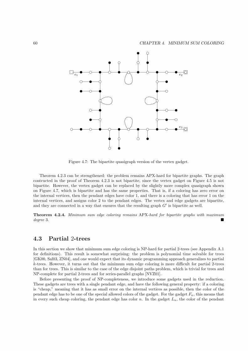
60 CHAPTER 4. MINIMUM SUM COLORING
e2
e3
e1
Figure 4.7: The bipartite quasigraph version of the vertex gadget.
Theorem 4.2.3 can be strengthened: the problem remains APX-hard for bipartite graphs. The graphcontructed in the proof of Theorem 4.2.3 is not bipartite, since the vertex gadget on Figure 4.5 is notbipartite. However, the vertex gadget can be replaced by the slightly more complex quasigraph shownon Figure 4.7, which is bipartite and has the same properties. That is, if a coloring has zero error onthe internal vertices, then the pendant edges have color 1, and there is a coloring that has error 1 on theinternal vertices, and assigns color 2 to the pendant edges. The vertex and edge gadgets are bipartite,and they are connected in a way that ensures that the resulting graph G′ is bipartite as well.
Theorem 4.2.4. Minimum sum edge coloring remains APX-hard for bipartite graphs with maximumdegree 3. �
4.3 Partial 2-trees
In this section we show that minimum sum edge coloring is NP-hard for partial 2-trees (see Appendix A.1for definitions). This result is somewhat surprising: the problem is polynomial time solvable for trees[GK00, Sal03, ZN04], and one would expect that its dynamic programming approach generalizes to partialk-trees. However, it turns out that the minimum sum edge coloring is more difficult for partial 2-treesthan for trees. This is similar to the case of the edge disjoint paths problem, which is trivial for trees andNP-complete for partial 2-trees and for series-parallel graphs [NVZ01].
Before presenting the proof of NP-completeness, we introduce some gadgets used in the reduction.These gadgets are trees with a single pendant edge, and have the following general property: if a coloringis “cheap,” meaning that it has as small error on the internal vertices as possible, then the color of thependant edge has to be one of the special allowed colors of the gadget. For the gadget Fn, this means thatin every such cheap coloring, the pendant edge has color n. In the gadget Ln, the color of the pendant
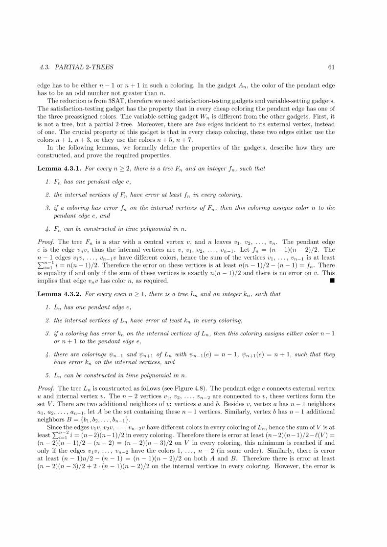
4.3. PARTIAL 2-TREES 61
edge has to be either n− 1 or n+ 1 in such a coloring. In the gadget An, the color of the pendant edgehas to be an odd number not greater than n.
The reduction is from 3SAT, therefore we need satisfaction-testing gadgets and variable-setting gadgets.The satisfaction-testing gadget has the property that in every cheap coloring the pendant edge has one ofthe three preassigned colors. The variable-setting gadget Wn is different from the other gadgets. First, itis not a tree, but a partial 2-tree. Moreover, there are two edges incident to its external vertex, insteadof one. The crucial property of this gadget is that in every cheap coloring, these two edges either use thecolors n+ 1, n+ 3, or they use the colors n+ 5, n+ 7.
In the following lemmas, we formally define the properties of the gadgets, describe how they areconstructed, and prove the required properties.
Lemma 4.3.1. For every n ≥ 2, there is a tree Fn and an integer fn, such that
1. Fn has one pendant edge e,
2. the internal vertices of Fn have error at least fn in every coloring,
3. if a coloring has error fn on the internal vertices of Fn, then this coloring assigns color n to thependant edge e, and
4. Fn can be constructed in time polynomial in n.
Proof. The tree Fn is a star with a central vertex v, and n leaves v1, v2, . . . , vn. The pendant edgee is the edge vnv, thus the internal vertices are v, v1, v2, . . . , vn−1. Let fn = (n − 1)(n − 2)/2. Then − 1 edges v1v, . . . , vn−1v have different colors, hence the sum of the vertices v1, . . . , vn−1 is at least∑n−1
i=1 i = n(n− 1)/2. Therefore the error on these vertices is at least n(n − 1)/2 − (n− 1) = fn. Thereis equality if and only if the sum of these vertices is exactly n(n − 1)/2 and there is no error on v. Thisimplies that edge vnv has color n, as required. �
Lemma 4.3.2. For every even n ≥ 1, there is a tree Ln and an integer kn, such that
1. Ln has one pendant edge e,
2. the internal vertices of Ln have error at least kn in every coloring,
3. if a coloring has error kn on the internal vertices of Ln, then this coloring assigns either color n− 1or n+ 1 to the pendant edge e,
4. there are colorings ψn−1 and ψn+1 of Ln with ψn−1(e) = n − 1, ψn+1(e) = n + 1, such that theyhave error kn on the internal vertices, and
5. Ln can be constructed in time polynomial in n.
Proof. The tree Ln is constructed as follows (see Figure 4.8). The pendant edge e connects external vertexu and internal vertex v. The n − 2 vertices v1, v2, . . . , vn−2 are connected to v, these vertices form theset V . There are two additional neighbors of v: vertices a and b. Besides v, vertex a has n− 1 neighborsa1, a2, . . . , an−1, let A be the set containing these n− 1 vertices. Similarly, vertex b has n− 1 additionalneighbors B = {b1, b2, . . . , bn−1}.
Since the edges v1v, v2v, . . . , vn−2v have different colors in every coloring of Ln, hence the sum of V is atleast
∑n−2i=1 i = (n−2)(n−1)/2 in every coloring. Therefore there is error at least (n−2)(n−1)/2−ℓ(V ) =
(n − 2)(n − 1)/2 − (n − 2) = (n − 2)(n − 3)/2 on V in every coloring, this minimum is reached if andonly if the edges v1v, . . . , vn−2 have the colors 1, . . . , n − 2 (in some order). Similarly, there is errorat least (n − 1)n/2 − (n − 1) = (n − 1)(n − 2)/2 on both A and B. Therefore there is error at least(n − 2)(n − 3)/2 + 2 · (n − 1)(n − 2)/2 on the internal vertices in every coloring. However, the error is
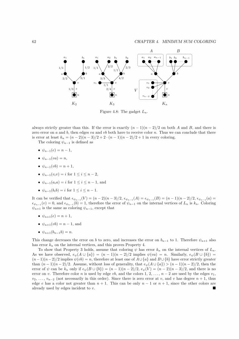
62 CHAPTER 4. MINIMUM SUM COLORING
BA
V
KnK2 K3
1/1
2/3
4/2
2/4
3/3
2/2
1/3
3/1
1/2
2/2
1/1 1/11/1
v1v1
v2
vn−2
. . .. . .
.
.
.
vv v
a1a1 a1 a2a2 an−1 b1b1b1 b2b2 bn−1
aaa bbb
u uu
e ee
Figure 4.8: The gadget Ln.
always strictly greater than this. If the error is exactly (n − 1)(n− 2)/2 on both A and B, and there iszero error on a and b, then edges va and vb both have to receive color n. Thus we can conclude that thereis error at least kn = (n− 2)(n− 3)/2 + 2 · (n− 1)(n− 2)/2 + 1 in every coloring.
The coloring ψn−1 is defined as
• ψn−1(e) = n− 1,
• ψn−1(va) = n,
• ψn−1(vb) = n+ 1,
• ψn−1(viv) = i for 1 ≤ i ≤ n− 2,
• ψn−1(aia) = i for 1 ≤ i ≤ n− 1, and
• ψn−1(bib) = i for 1 ≤ i ≤ n− 1.
It can be verified that ǫψn−1(V ) = (n− 2)(n− 3)/2, ǫψn−1(A) = ǫψn−1(B) = (n− 1)(n− 2)/2, ǫψn−1(a) =ǫψn−1(v) = 0, and ǫψn−1(b) = 1, therefore the error of ψn−1 on the internal vertices of Ln is kn. Coloringψn+1 is the same as coloring ψn−1, except that
• ψn+1(e) = n+ 1,
• ψn+1(vb) = n− 1, and
• ψn+1(bn−1b) = n.
This change decreases the error on b to zero, and increases the error on bn−1 to 1. Therefore ψn+1 alsohas error kn on the internal vertices, and this proves Property 4.
To show that Property 3 holds, assume that coloring ψ has error kn on the internal vertices of Ln.As we have observed, eψ(A ∪ {a}) = (n − 1)(n − 2)/2 implies ψ(va) = n. Similarly, eψ(B ∪ {b}) =(n−1)(n−2)/2 implies ψ(vb) = n, therefore at least one of A∪{a} and B∪{b} have error strictly greaterthan (n− 1)(n− 2)/2. Assume, without loss of generality, that eψ(A ∪ {a}) > (n− 1)(n− 2)/2, then theerror of ψ can be kn only if eψ(B ∪ {b}) = (n − 1)(n − 2)/2, eψ(V ) = (n − 2)(n − 3)/2, and there is noerror on v. Therefore color n is used by edge vb, and the colors 1, 2, . . . , n− 2 are used by the edges v1,v2, . . . , vn−2 (not necessarily in this order). Since there is zero error at v, and v has degree n + 1, thusedge e has a color not greater than n + 1. This can be only n − 1 or n + 1, since the other colors arealready used by edges incident to v. �

4.3. PARTIAL 2-TREES 63
3/1/1
1/3/5
F4
K4F2
K2
v
e
w2
w4v2
v4
u
5/5/32/2/
2
4/4/4
Figure 4.9: The gadget A5.
Lemma 4.3.3. For every odd n ≥ 1, there is a tree An and an integer an such that
1. An has one pendant edge e,
2. the internal vertices of An have error at least an in every coloring,
3. if a coloring ψ has error an on the internal vertices of An, then ψ(e) is odd and ψ(e) ≤ n,
4. for every odd c not greater than n, there is a coloring ψc of An such that ψc(e) = c and it has erroran on the internal vertices,
5. An can be constructed in time polynomial in n.
Proof. The pendant edge e of Ln connects external vertex u and internal vertex v. Attach the pendantedges of the (n − 1)/2 trees F2, F4, . . . , Fn−1 (Lemma 4.3.1) to vertex v, let the pendant edges of thesetrees be v2v, v4v, . . . , vn−1v, respectively (see Figure 4.9). Similarly, attach the pendant edges of the(n − 1)/2 trees L2, L4, . . . , Ln−1 (Lemma 4.3.2) to v, let the pendant edges of these trees be w2v, w4v,. . . , wn−1v, respectively. Therefore the degree of v in An is n.
Let an = (f2 + f4 + · · ·+ fn−1) + (k2 + k4 + · · ·+ kn−1). Since An contains a copy of the trees F2, F4,. . . , Fn−1, and a copy of the trees L2, L4, . . . , Ln−1, thus it is clear that every coloring of An has at leastan errors on the internal vertices. Moreover, if a coloring ψ has error an on the internal vertices, thenψ(viv) = i for i = 2, 4, . . . , n− 1, and the error of v is zero. This implies that ψ(e) ≤ n and not even, asrequired.
The coloring ψc required by Property 4 is the following. For every i = 2, 4, . . . , n−1, coloring ψc colorsthe edges of the tree Fi in such a way that the pendant edge viv receives color i, and there is error fi onthe internal vertices of Fi, by Lemma 4.3.1, there is such a coloring. For every i = 2, 4, . . . , c− 1, the treeLi is colored such that the pendant edge wiv has color i− 1, and there is error ki on the internal verticesof Li. Similarly, for i = c+ 1, . . . , n− 1, the tree Li is colored such that the pendant edge wiv has colori+ 1, and there is error ki on the internal vertices of Li. Coloring ψc assigns color c to edge e, thus everycolor 1, 2, . . . , n appears on exactly one edge incident to v. Therefore the error of v is zero, and there iserror an on the internal vertices of An. �
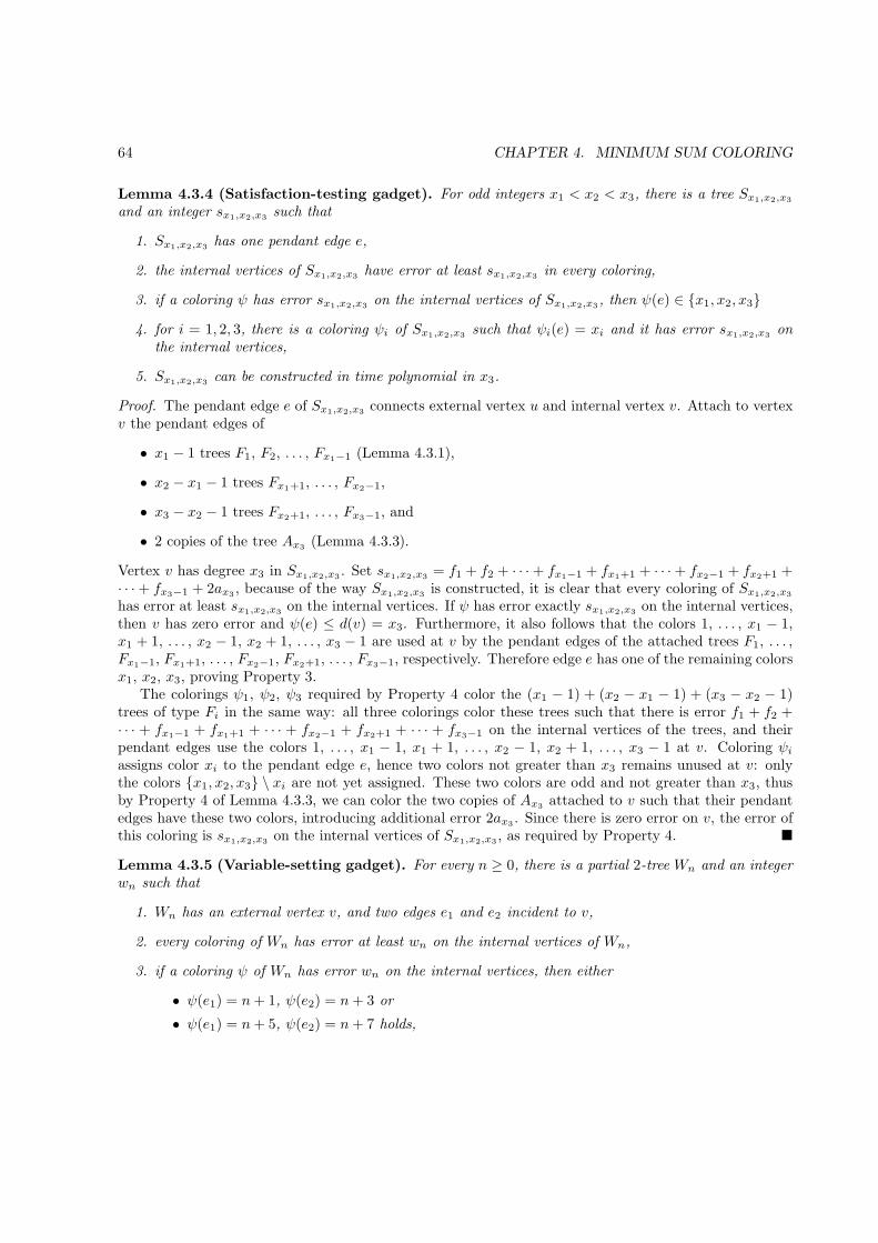
64 CHAPTER 4. MINIMUM SUM COLORING
Lemma 4.3.4 (Satisfaction-testing gadget). For odd integers x1 < x2 < x3, there is a tree Sx1,x2,x3
and an integer sx1,x2,x3 such that
1. Sx1,x2,x3 has one pendant edge e,
2. the internal vertices of Sx1,x2,x3 have error at least sx1,x2,x3 in every coloring,
3. if a coloring ψ has error sx1,x2,x3 on the internal vertices of Sx1,x2,x3 , then ψ(e) ∈ {x1, x2, x3}
4. for i = 1, 2, 3, there is a coloring ψi of Sx1,x2,x3 such that ψi(e) = xi and it has error sx1,x2,x3 onthe internal vertices,
5. Sx1,x2,x3 can be constructed in time polynomial in x3.
Proof. The pendant edge e of Sx1,x2,x3 connects external vertex u and internal vertex v. Attach to vertexv the pendant edges of
• x1 − 1 trees F1, F2, . . . , Fx1−1 (Lemma 4.3.1),
• x2 − x1 − 1 trees Fx1+1, . . . , Fx2−1,
• x3 − x2 − 1 trees Fx2+1, . . . , Fx3−1, and
• 2 copies of the tree Ax3 (Lemma 4.3.3).
Vertex v has degree x3 in Sx1,x2,x3 . Set sx1,x2,x3 = f1 + f2 + · · · + fx1−1 + fx1+1 + · · · + fx2−1 + fx2+1 +· · · + fx3−1 + 2ax3 , because of the way Sx1,x2,x3 is constructed, it is clear that every coloring of Sx1,x2,x3
has error at least sx1,x2,x3 on the internal vertices. If ψ has error exactly sx1,x2,x3 on the internal vertices,then v has zero error and ψ(e) ≤ d(v) = x3. Furthermore, it also follows that the colors 1, . . . , x1 − 1,x1 + 1, . . . , x2 − 1, x2 + 1, . . . , x3 − 1 are used at v by the pendant edges of the attached trees F1, . . . ,Fx1−1, Fx1+1, . . . , Fx2−1, Fx2+1, . . . , Fx3−1, respectively. Therefore edge e has one of the remaining colorsx1, x2, x3, proving Property 3.
The colorings ψ1, ψ2, ψ3 required by Property 4 color the (x1 − 1) + (x2 − x1 − 1) + (x3 − x2 − 1)trees of type Fi in the same way: all three colorings color these trees such that there is error f1 + f2 +· · · + fx1−1 + fx1+1 + · · · + fx2−1 + fx2+1 + · · · + fx3−1 on the internal vertices of the trees, and theirpendant edges use the colors 1, . . . , x1 − 1, x1 + 1, . . . , x2 − 1, x2 + 1, . . . , x3 − 1 at v. Coloring ψiassigns color xi to the pendant edge e, hence two colors not greater than x3 remains unused at v: onlythe colors {x1, x2, x3} \ xi are not yet assigned. These two colors are odd and not greater than x3, thusby Property 4 of Lemma 4.3.3, we can color the two copies of Ax3 attached to v such that their pendantedges have these two colors, introducing additional error 2ax3 . Since there is zero error on v, the error ofthis coloring is sx1,x2,x3 on the internal vertices of Sx1,x2,x3 , as required by Property 4. �
Lemma 4.3.5 (Variable-setting gadget). For every n ≥ 0, there is a partial 2-tree Wn and an integerwn such that
1. Wn has an external vertex v, and two edges e1 and e2 incident to v,
2. every coloring of Wn has error at least wn on the internal vertices of Wn,
3. if a coloring ψ of Wn has error wn on the internal vertices, then either
• ψ(e1) = n+ 1, ψ(e2) = n+ 3 or
• ψ(e1) = n+ 5, ψ(e2) = n+ 7 holds,
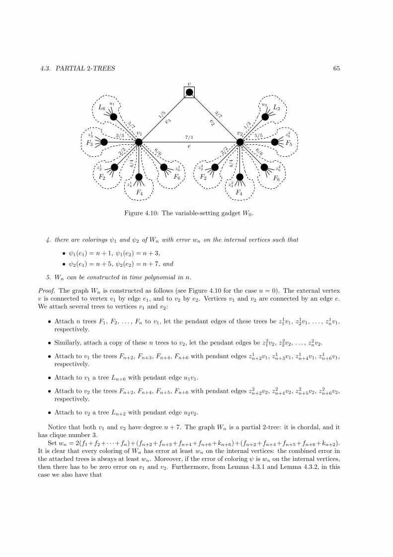
4.3. PARTIAL 2-TREES 65
e25/7
3/3
1/5
F3
L6 L2
F5
F4F4
F2F2 F6
3/7
7/1
4/4
4/4
2/2
2/2 6/6
6/6
e 1
v1 v2
e
v
F6
z12
z14
z16
u1
z13
z24
z26
z25
u2
z22
5/5
1/3
Figure 4.10: The variable-setting gadget W0.
4. there are colorings ψ1 and ψ2 of Wn with error wn on the internal vertices such that
• ψ1(e1) = n+ 1, ψ1(e2) = n+ 3,
• ψ2(e1) = n+ 5, ψ2(e2) = n+ 7, and
5. Wn can be constructed in time polynomial in n.
Proof. The graph Wn is constructed as follows (see Figure 4.10 for the case n = 0). The external vertexv is connected to vertex v1 by edge e1, and to v2 by e2. Vertices v1 and v2 are connected by an edge e.We attach several trees to vertices v1 and v2:
• Attach n trees F1, F2, . . . , Fn to v1, let the pendant edges of these trees be z11v1, z1
2v1, . . . , z1nv1,
respectively.
• Similarly, attach a copy of these n trees to v2, let the pendant edges be z21v2, z2
2v2, . . . , z2nv2.
• Attach to v1 the trees Fn+2, Fn+3, Fn+4, Fn+6 with pendant edges z1n+2v1, z1
n+3v1, z1n+4v1, z1
n+6v1,respectively.
• Attach to v1 a tree Ln+6 with pendant edge u1v1.
• Attach to v2 the trees Fn+2, Fn+4, Fn+5, Fn+6 with pendant edges z2n+2v2, z2
n+4v2, z2n+5v2, z2
n+6v2,respectively.
• Attach to v2 a tree Ln+2 with pendant edge u2v2.
Notice that both v1 and v2 have degree n+ 7. The graph Wn is a partial 2-tree: it is chordal, and ithas clique number 3.
Set wn = 2(f1+f2 + · · ·+fn)+(fn+2 +fn+3+fn+4+fn+6+kn+6)+(fn+2 +fn+4+fn+5+fn+6 +kn+2).It is clear that every coloring of Wn has error at least wn on the internal vertices: the combined error inthe attached trees is always at least wn. Moreover, if the error of coloring ψ is wn on the internal vertices,then there has to be zero error on v1 and v2. Furthermore, from Lemma 4.3.1 and Lemma 4.3.2, in thiscase we also have that
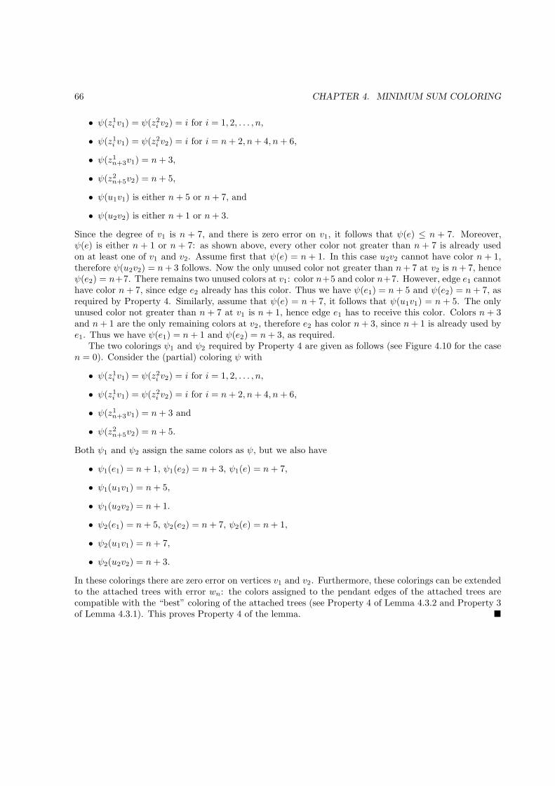
66 CHAPTER 4. MINIMUM SUM COLORING
• ψ(z1i v1) = ψ(z2
i v2) = i for i = 1, 2, . . . , n,
• ψ(z1i v1) = ψ(z2
i v2) = i for i = n+ 2, n+ 4, n+ 6,
• ψ(z1n+3v1) = n+ 3,
• ψ(z2n+5v2) = n+ 5,
• ψ(u1v1) is either n+ 5 or n+ 7, and
• ψ(u2v2) is either n+ 1 or n+ 3.
Since the degree of v1 is n + 7, and there is zero error on v1, it follows that ψ(e) ≤ n + 7. Moreover,ψ(e) is either n + 1 or n + 7: as shown above, every other color not greater than n + 7 is already usedon at least one of v1 and v2. Assume first that ψ(e) = n+ 1. In this case u2v2 cannot have color n + 1,therefore ψ(u2v2) = n+ 3 follows. Now the only unused color not greater than n+ 7 at v2 is n+ 7, henceψ(e2) = n+7. There remains two unused colors at v1: color n+5 and color n+7. However, edge e1 cannothave color n+ 7, since edge e2 already has this color. Thus we have ψ(e1) = n+ 5 and ψ(e2) = n+ 7, asrequired by Property 4. Similarly, assume that ψ(e) = n + 7, it follows that ψ(u1v1) = n + 5. The onlyunused color not greater than n + 7 at v1 is n + 1, hence edge e1 has to receive this color. Colors n+ 3and n+ 1 are the only remaining colors at v2, therefore e2 has color n+ 3, since n+ 1 is already used bye1. Thus we have ψ(e1) = n+ 1 and ψ(e2) = n+ 3, as required.
The two colorings ψ1 and ψ2 required by Property 4 are given as follows (see Figure 4.10 for the casen = 0). Consider the (partial) coloring ψ with
• ψ(z1i v1) = ψ(z2
i v2) = i for i = 1, 2, . . . , n,
• ψ(z1i v1) = ψ(z2
i v2) = i for i = n+ 2, n+ 4, n+ 6,
• ψ(z1n+3v1) = n+ 3 and
• ψ(z2n+5v2) = n+ 5.
Both ψ1 and ψ2 assign the same colors as ψ, but we also have
• ψ1(e1) = n+ 1, ψ1(e2) = n+ 3, ψ1(e) = n+ 7,
• ψ1(u1v1) = n+ 5,
• ψ1(u2v2) = n+ 1.
• ψ2(e1) = n+ 5, ψ2(e2) = n+ 7, ψ2(e) = n+ 1,
• ψ2(u1v1) = n+ 7,
• ψ2(u2v2) = n+ 3.
In these colorings there are zero error on vertices v1 and v2. Furthermore, these colorings can be extendedto the attached trees with error wn: the colors assigned to the pendant edges of the attached trees arecompatible with the “best” coloring of the attached trees (see Property 4 of Lemma 4.3.2 and Property 3of Lemma 4.3.1). This proves Property 4 of the lemma. �

4.3. PARTIAL 2-TREES 67
Theorem 4.3.6. Minimum sum edge coloring is NP-hard for partial 2-trees.
Proof. The proof is by reduction from 3SAT: given a 3CNF formula ϕ, we construct a partial 2-tree Gand determine an integer K such that Σ′(G) ≤ K if and only if ϕ is satisfiable. By Prop. 2.1.3, we canassume that every variable occurs exactly twice positively and exactly twice negated in φ, and every clausecontains exactly three literals.
Let n be the number of variables in ϕ, the variables will be called x0, x1, . . . , xn−1. The number ofclauses is therefore m = 4n/3. For every literal of ϕ, there is a corresponding color, as follows:
• color 8i+ 1 corresponds to the first positive occurence of xi,
• color 8i+ 3 corresponds to the second positive occurence of xi,
• color 8i+ 5 corresponds to the first negated occurence of xi, and
• color 8i+ 7 corresponds to the second negated occurence of xi.
Notice that these numbers are odd, and every odd number not greater than 8n corresponds to a literal.Take a vertex v, we will attach several gadgets to v to obtain the graph G. Attach 4n trees F2, F4,
. . . , F8n to v, let the pendant edges of the attached trees be u2v, u4v, . . . , u8nv, respectively. Attach nvariable-setting gadgets W0, W8, W16, . . . , W8(n−1) to v, let the two edges of W8i incident to v be calledwi,1v and wi,2v. For every clause Cj of ϕ, we attach a satisfaction-testing gadget to v in the followingway: if colors cj,1 < cj,2 < cj,3 correspond to the three literals in clause Cj , then attach a tree Sc1,c2,c3to v, and let sjv be its pendant edge. Finally, attach m/2 copies of the tree A8n−1 to v, let the pendantedges of these trees be t1v, t2v, . . . , tm
2v. This completes the description of the graph G. Since every
gadget is a partial 2-tree (or even a tree), the graph G is a partial 2-tree as well: joining graphs at a singlevertex does not increase the treewidth of the graphs.
Let K(1) = f2 +f4+ · · ·+f8n. In every coloring of G the error is at least K(1) on the internal vertices ofthe 4n attached Fi trees. Let K(2) = w0 +w8 + · · ·+w8(n−1). In every coloring the error is at least K(2) on
the internal vertices of the n variable-setting gadgets. Let K(3) = m/2 · a8n−1. In every coloring the erroris at least K(3) on the internal vertices of the m/2 copies of A8n−1. Let K(4) =
∑mj=1 scj,1,cj,2,cj,3 where cj,k
is the color corresponding to the kth literal in clause Cj . In every coloring of G, the error on the internalvertices of the m satisfaction-testing gadget is at least K(4). Finally, set K = K(1) +K(2) +K(3) +K(4).It is clear that every coloring of G has error at least K. We claim that G has a coloring with error exactlyK if and only if ϕ is satisfiable.
Assume first that coloring ψ has error K. This is possible only if ψ has zero error on v, and thereis exactly K error on the internal vertices of the attached gadgets. By Lemma 4.3.1, Lemma 4.3.3,Lemma 4.3.4, and Lemma 4.3.5 this implies that
• ψ(uiv) = i for i = 2, 4, . . . , 8n,
• for every i = 0, 1, . . . , n− 1, either
– ψ(wi,1v) = 8i+ 1 and ψ(wi,2v) = 8i+ 3, or
– ψ(wi,1v) = 8i+ 5 and ψ(wi,2v) = 8i+ 7,
• ψ(sjv) ∈ {cj,1, cj,2, cj,3} for every j = 1, . . . , m, and
• ψ(tiv) ≤ 8n− 1 and odd for every i = 1, 2, . . . , m/2.
Consider the following variable assignment: set variable xi to true if ψ(wi,1v) = 8i+ 5, ψ(wi,2v) = 8i+ 7,and set xi to false if ψ(wi,1v) = 8i+ 1 and ψ(wi,2v) = 8i+ 3. We show that this is a satisfying assignmentof ϕ, every clause Cj is satisfied. Assume that ψ(sjv) = cj,k for some k = 1, 2, 3, and let the kth literalin clause Cj be an occurence of the variable xi. In this case, the kth literal of clause Cj is true in the
68 CHAPTER 4. MINIMUM SUM COLORING
32
1
1
1
1
1
1
Figure 4.11: A tree with strength 3. The figure shows a minimum sum coloring with sum 11, while every2-coloring has sum 12.
constructed variable assignment: otherwise color cj,w would appear also on edge wi,1v or wi,2v. Thereforeevery clause contains at least one true literal, and the formula is satisfied by the variable assignment.
Now assume that ϕ has a satisfying variable assignment. Consider the following (partial) coloring ψ:
• ψ(uiv) = i for i = 2, 4, . . . , 8n,
• for every i = 0, 1, . . . , n− 1,
– if variable xi is true, then ψ(wi,1v) = 8i+ 5 and ψ(wi,2v) = 8i+ 7,
– if variable xi false, then ψ(wi,1v) = 8i+ 1 and ψ(wi,2v) = 8i+ 3,
It is clear from the construction that for every j = 1, 2, . . . , m, one of the colors cj,1, cj,2, cj,3 is notalready assigned: otherwise this would imply that clause Cj contains only false literals in the satisfyingvariable assignment, a contradiction. Therefore we can set ψ(sjv) to one of these three colors. So farcoloring ψ assigns 4n even and 2n + m odd colors to the edges incident to v, therefore there remainsexactly m/2 odd colors not greater than 8n. Assign these colors to the edges t1v, t2v, . . . , tm
2v in some
order. Now every color not greater than 8n is used exactly once at v, hence there is zero error on vertexv in ψ. It is straightforward to verify that this coloring can be extended to the whole graph G such thatthe resulting coloring has error exactly K: in every gadget, the edges incident to v are colored in such away that makes this extension possible. �
4.4 Chromatic strength
In [KS89] it is noted that the number of colors required by a minimum sum coloring can be much greaterthan the chromatic number of the graph. In particular, for every k ≥ 2, they show a tree where everyminimum sum coloring uses at least k different colors (see Figure 4.11 for an example of the case k = 3).Let s(G) be the chromatic strength of G, which is the smallest number of colors required in a minimumsum coloring of G. The chromatic edge strength s′(G) is defined analogously. Clearly, s(G) ≥ χ(G), butas the trees in [KS89] show, s(G) − χ(G) can be arbitrarily large. On the other hand, [MMS97] andindependently [HMT00] prove an analog of Vizing’s Theorem showing that s′(G) ≤ ∆(G) + 1 in everysimple graph G. Hence we have
∆(G) ≤ χ′(G) ≤ s′(G) ≤ ∆(G) + 1
if G is a simple graph. Harary and Plantholt conjectured (see [Wes95]) that the second inequality is infact an equality, hence if a simple graph is k-edge-colorable, then it has a minimum sum edge coloringwith k colors. However, this conjecture turned out to be false: for every odd integer k ≥ 5, a graph withchromatic index k and edge strength k+ 1 was given in [MMS97]. Moreover, [HMT00] gives such a graphfor k = 4. Thus we can conclude that the chromatic index and the chromatic edge strength are not alwaysthe same.
4.4. CHROMATIC STRENGTH 69
Here we study the computational complexity of determining the chromatic strength and chromaticedge strength of a simple graph. The complexity of the vertex strength is investigated in [Sal03]:
Theorem 4.4.1 ([Sal03]). For every k ≥ 3, it is NP-hard to decide whether s(G) ≤ k holds for a givengraph G.
Notice that it is not clear whether this problem belongs to NP. A minimum sum k-coloring is not agood certificate for s(G) ≤ k, since we cannot verify that it is indeed a minimum sum coloring. On theother hand, the problem does not seem to belong to coNP either: a minimum sum coloring with more thank colors does not certify that s(G) > k, since it does not prove that this sum cannot be achieved usingonly k colors. The main result of this chapter is that we determine the exact complexity of the chromaticstrength problem by showing that for every k ≥ 3, it is Θp
2-complete to decide whether s(G) ≤ k holds.The class Θp
2 contains those problems that can be solved in polynomial time with a logarithmic numberof NP oracle calls (see Appendix A.3 and Section 4.4.3 for definitions). It is interesting to see a naturalcoloring problem that is complete for this less-known complexity class. In [Sal03] the complexity of thecase k = 2 was left as an open question. We answer this question by showing that deciding s(G) ≤ 2 iscoNP-complete.
We obtain our Θp2-completeness result for the chromatic strength by proving the stronger statement
that even the more restricted chromatic edge strength problem is Θp2-complete. The complexity of edge
strength is also treated in [Sal03]. By observing that s′(G) = χ′(G) for every regular simple graph, theyconclude that for regular graphs “Is s′(G) ≤ k?” has the same complexity as “Is χ′(G) ≤ k?”, and thelatter problem is known to be NP-complete for every k ≥ 3 [Hol81, LG83]. However, if we want to provethat edge strength is Θp
2-complete (that is, harder than the chromatic index problem), then necessarilywe have to consider graphs where the edge strength and the chromatic index are not the same. Thereforewe need substantially different (and more complicated) arguments than in [Sal03].
We prove the Θp2-completeness of chromatic edge strength the following way. First we show that
for every k ≥ 3, there is a simple graph Gk with ∆(Gk) = χ′(Gk) = k and s′(Gk) = k + 1. That is,we give counterexamples to the conjecture of Harary and Plantholt in all the remaining cases. Next,in Section 4.4.3 we introduce some new Θp
2-complete problems, which might be of independent interestas well. In particular, we show that it is Θp
2-complete to decide whether every minimum vertex coverof a given graph includes the distinguished vertex v. Finally, we show that if the chromatic index andthe chromatic edge strength are not always the same in graphs with maximum degree k, then it is Θp
2-complete to decide whether the edge strength is k in such a graph. Together with the existence of thecounterexample graphs, this gives the required result.
In Section 4.4.1, we show that it is coNP-complete to decide whether s(G) ≤ 2. In the rest ofthe chapter, we consider only the edge coloring version of the problem. The counterexamples to theconjecture of Harary and Plantholt are given in Section 4.4.2. In Section 4.4.3 we summarize the resultson the complexity class Θp
2, and introduce the new Θp2-complete problems. The reduction for the main
hardness result is presented in Section 4.4.4. The construction of the key gadget of the reduction is givenin Section 4.4.5.
4.4.1 Vertex strength of bipartite graphs
In this section we prove that for k = 2, it is coNP-complete to decide whether s(G) ≤ k holds. Noticethat, unlike in the case k ≥ 3, now it is easy to see that the problem is in coNP. First, the question makessense only if the graph is bipartite, otherwise trivially s(G) ≥ 3. In a bipartite graph the sum of the best2-coloring is easy to determine: each connected component of the graph has exactly two 2-colorings, andtaking the better coloring of each component gives the best 2-coloring of the graph. Therefore a minimumsum coloring with more than 2 colors certifies that s(G) ≤ 2 does not hold: one can determine the sumof the best 2-coloring, and check that it is indeed larger than the sum of the given coloring. Thus theproblem is in coNP.
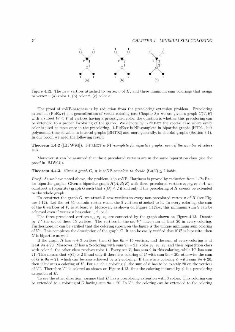
70 CHAPTER 4. MINIMUM SUM COLORING
3
(b)2 2
1
1 1 1 1
2
(a)
v vv
11 11
22
1
(c)
22
Figure 4.12: The new vertices attached to vertex v of H , and three minimum sum colorings that assignto vertex v (a) color 1, (b) color 2, (c) color 3.
The proof of coNP-hardness is by reduction from the precoloring extension problem. Precoloringextension (PrExt) is a generalization of vertex coloring (see Chapter 3): we are given a graph G(V,E)with a subset W ⊆ V of vertices having a preassigned color, the question is whether this precoloring canbe extended to a proper k-coloring of the graph. We denote by 1-PrExt the special case where everycolor is used at most once in the precoloring. 1-PrExt is NP-complete in bipartite graphs [HT93], butpolynomial-time solvable in interval graphs [BHT92] and more generally, in chordal graphs (Section 3.1).In our proof, we need the following result:
Theorem 4.4.2 ([BJW94]). 1-PrExt is NP-complete for bipartite graphs, even if the number of colorsis 3.
Moreover, it can be assumed that the 3 precolored vertices are in the same bipartition class (see theproof in [BJW94]).
Theorem 4.4.3. Given a graph G, it is coNP-complete to decide if s(G) ≤ 2 holds.
Proof. As we have noted above, the problem is in coNP. Hardness is proved by reduction from 1-PrExt
for bipartite graphs. Given a bipartite graph H(A,B;E) with three precolored vertices v1, v2, v3 ∈ A, weconstruct a (bipartite) graph G such that s(G) ≤ 2 if and only if the precoloring of H cannot be extendedto the whole graph.
To construct the graph G, we attach 5 new vertices to every non-precolored vertex v of H (see Fig-ure 4.12). Let the set Vv contain vertex v and the 5 vertices attached to it. In every coloring, the sumof the 6 vertices of Vv is at least 9. Moreover, as shown on Figure 4.12a-c, this minimum sum 9 can beachieved even if vertex v has color 1, 2, or 3.
The three precolored vertices v1, v2, v3 are connected by the graph shown on Figure 4.13. Denoteby V ∗ the set of these 15 vertices. The vertices in the set V ∗ have sum at least 20 in every coloring.Furthermore, it can be verified that the coloring shown on the figure is the unique minimum sum coloringof V ∗. This completes the description of the graph G. It can be easily verified that if H is bipartite, thenG is bipartite as well.
If the graph H has n + 3 vertices, then G has 6n + 15 vertices, and the sum of every coloring is atleast 9n+ 20. Moreover, G has a 2-coloring with sum 9n+ 21: color v1, v2, v3, and their bipartition classwith color 2, the other class receives color 1. Every set Vv has sum 9 in this coloring, while V ∗ has sum21. This means that s(G) > 2 if and only if there is a coloring of G with sum 9n+ 20: otherwise the sumof G is 9n + 21, which can be also achieved by a 2-coloring. If there is a coloring ψ with sum 9n + 20,then it induces a coloring of H . For a such a coloring ψ, the sum of ψ has to be exactly 20 on the verticesof V ∗. Therefore V ∗ is colored as shown on Figure 4.13, thus the coloring induced by ψ is a precoloringextension of H .
To see the other direction, assume that H has a precoloring extension with 3 colors. This coloring canbe extended to a coloring of G having sum 9n+ 20. In V ∗, the coloring can be extended to the coloring
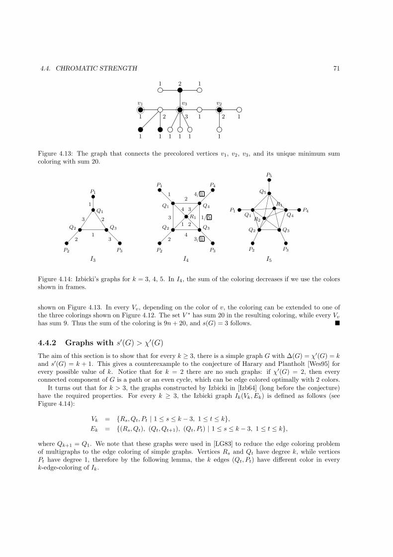
4.4. CHROMATIC STRENGTH 71
11
v3
32 2
v2v1
1
1
1 1 1 1 1
11
2
Figure 4.13: The graph that connects the precolored vertices v1, v2, v3, and its unique minimum sumcoloring with sum 20.
3/ 1
1/ 5
4/ 1
1
Q1
1
P1
P1
22
2
P4
4
2
4
2
3
3
3
31
1
P2P2P2 P3P3P3
P5
P4P1
Q2Q2Q2 Q3
Q3Q3
Q4
Q4
Q1
Q1
Q5
R1
R1 R2
I3 I4 I5
Figure 4.14: Izbicki’s graphs for k = 3, 4, 5. In I4, the sum of the coloring decreases if we use the colorsshown in frames.
shown on Figure 4.13. In every Vv, depending on the color of v, the coloring can be extended to one ofthe three colorings shown on Figure 4.12. The set V ∗ has sum 20 in the resulting coloring, while every Vvhas sum 9. Thus the sum of the coloring is 9n+ 20, and s(G) = 3 follows. �
4.4.2 Graphs with s′(G) > χ′(G)
The aim of this section is to show that for every k ≥ 3, there is a simple graph G with ∆(G) = χ′(G) = kand s′(G) = k + 1. This gives a counterexample to the conjecture of Harary and Plantholt [Wes95] forevery possible value of k. Notice that for k = 2 there are no such graphs: if χ′(G) = 2, then everyconnected component of G is a path or an even cycle, which can be edge colored optimally with 2 colors.
It turns out that for k > 3, the graphs constructed by Izbicki in [Izb64] (long before the conjecture)have the required properties. For every k ≥ 3, the Izbicki graph Ik(Vk, Ek) is defined as follows (seeFigure 4.14):
Vk = {Rs, Qt, Pt | 1 ≤ s ≤ k − 3, 1 ≤ t ≤ k},
Ek = {(Rs, Qt), (Qt, Qt+1), (Qt, Pt) | 1 ≤ s ≤ k − 3, 1 ≤ t ≤ k},
where Qk+1 = Q1. We note that these graphs were used in [LG83] to reduce the edge coloring problemof multigraphs to the edge coloring of simple graphs. Vertices Rs and Qt have degree k, while verticesPt have degree 1, therefore by the following lemma, the k edges (Qt, Pt) have different color in everyk-edge-coloring of Ik.
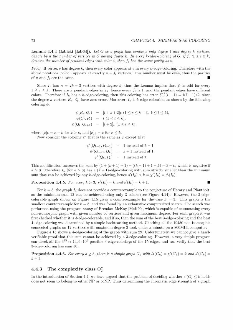
72 CHAPTER 4. MINIMUM SUM COLORING
Lemma 4.4.4 (Izbicki [Izb64]). Let G be a graph that contains only degree 1 and degree k vertices,denote by n the number of vertices in G having degree k. In every k-edge-coloring of G, if fi (1 ≤ i ≤ k)denotes the number of pendant edges with color i, then fi has the same parity as n.
Proof. If vertex v has degree k, then every color appears at v in every k-edge-coloring. Therefore with theabove notations, color i appears at exactly n+ fi vertices. This number must be even, thus the paritiesof n and fi are the same. �
Since Ik has n = 2k − 3 vertices with degree k, thus the Lemma implies that fi is odd for every1 ≤ i ≤ k. There are k pendant edges in Ik, hence every fi is 1, and the pendant edges have differentcolors. Therefore if Ik has a k-edge-coloring, then this coloring has error
∑ki (i − 1) = i(i − 1)/2, since
the degree k vertices Rs, Qt have zero error. Moreover, Ik is k-edge-colorable, as shown by the followingcoloring ψ:
ψ(Rs, Qt) = [t+ s+ 2]k (1 ≤ s ≤ k − 3, 1 ≤ t ≤ k),
ψ(Qt, Pt) = t (1 ≤ t ≤ k),
ψ(Qt, Qt+1) = [t+ 2]k (1 ≤ t ≤ k),
where [x]k = x− k for x > k, and [x]k = x for x ≤ k.Now consider the coloring ψ′ that is the same as ψ except that
ψ′(Qk−1, Pk−1) = 1 instead of k − 1,
ψ′(Qk−1, Qk) = k + 1 instead of 1,
ψ′(Qk, Pk) = 1 instead of k.
This modification increases the sum by (1 + (k + 1) + 1) − ((k − 1) + 1 + k) = 3 − k, which is negative ifk > 3. Therefore Ik (for k > 3) has a (k + 1)-edge-coloring with sum strictly smaller than the minimumsum that can be achieved by any k-edge-coloring, hence s′(Ik) > k = χ′(Ik) = ∆(Ik).
Proposition 4.4.5. For every k > 3, χ′(Ik) = k and s′(Ik) = k + 1. �
For k = 3, the graph I3 does not provide a counterexample to the conjecture of Harary and Plantholt,as the minimum sum 12 can be achieved using only 3 colors (see Figure 4.14). However, the 3-edge-colorable graph shown on Figure 4.15 gives a counterexample for the case k = 3. This graph is thesmallest counterexample for k = 3, and was found by an exhaustive computerized search. The search wasperformed using the program nauty of Brendan McKay [McK90], which is capable of enumerating everynon-isomorphic graph with given number of vertices and given maximum degree. For each graph it wasfirst checked whether it is 3-edge-colorable, and if so, then the sum of the best 3-edge-coloring and the best4-edge-coloring was determined by a simple backtracking method. Checking all the 19430 non-isomorphicconnected graphs on 12 vertices with maximum degree 3 took under a minute on a 800MHz computer.
Figure 4.15 shows a 4-edge-coloring of the graph with sum 29. Unfortunately, we cannot give a hand-verifiable proof that this sum cannot be achieved by a 3-edge-coloring. However, a very simple programcan check all the 315 ≈ 14.3 · 106 possible 3-edge-colorings of the 15 edges, and can verify that the best3-edge-coloring has sum 30.
Proposition 4.4.6. For every k ≥ 3, there is a simple graph Gk with ∆(Gk) = χ′(Gk) = k and s′(Gk) =k + 1.
4.4.3 The complexity class Θp2
In the introduction of Section 4.4, we have argued that the problem of deciding whether s′(G) ≤ k holdsdoes not seem to belong to either NP or coNP. Thus determining the chromatic edge strength of a graph
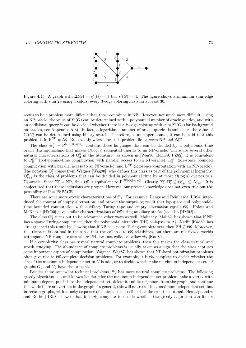
4.4. CHROMATIC STRENGTH 73
233
42
2
1
3
1
1
1
2
2
1
1
Figure 4.15: A graph with ∆(G) = χ′(G) = 3 but s′(G) = 4. The figure shows a minimum sum edgecoloring with sum 29 using 4 colors, every 3-edge-coloring has sum at least 30.
seems to be a problem more difficult than those contained in NP. However, not much more difficult: usingan NP-oracle, the value of Σ′(G) can be determined with a polynomial number of oracle queries, and withan additional query it can be decided whether there is a k-edge-coloring with sum Σ′(G) (for backgroundon oracles, see Appendix A.3). In fact, a logarithmic number of oracle queries is sufficient: the value ofΣ′(G) can be determined using binary search. Therefore, as an upper bound, it can be said that thisproblem is in PNP = ∆p
2. But exactly where does this problem lie between NP and ∆p2?
The class Θp2 = PNP[O(logn)] contains those languages that can be decided by a polynomial-time
oracle Turing-machine that makes O(log n) sequential queries to an NP-oracle. There are several othernatural characterizations of Θp
2 in the literature: as shown in [Wag90, Hem89, PZ82], it is equivalentto PNP
|| (polynomial-time computation with parallel access to an NP-oracle), LNP|| (log-space bounded
computation with parallel access to an NP-oracle), and LNP (log-space computation with an NP-oracle).The notation Θp
2 comes from Wagner [Wag90], who defines this class as part of the polynomial hierarchy:Θpi+1 is the class of problems that can be decided in polynomial time by at most O(log n) queries to a
Σpi -oracle. Since Σp1 = NP, thus Θp2 is equivalent to PNP[O(logn)]. Clearly, Σpi ,Π
pi ⊆ Θp
i+1 ⊆ ∆pi+1. It is
conjectured that these inclusions are proper. However, our present knowledge does not even rule out thepossibility of P = PSPACE.
There are some more exotic characterizations of Θp2. For example, Lange and Reinhardt [LR94] intro-
duced the concept of empty alternation, and proved the surprising result that log-space and polynomial-time bounded computation with auxiliary Turing tape and empty alternation equals Θp
2. Holzer andMcKenzie [HM00] gave similar characterizations of Θp
2 using auxiliary stacks (see also [HM02]).
The class Θp2 turns out to be relevant in other ways as well. Mahaney [Mah82] has shown that if NP
has a sparse Turing-complete set, then the polynomial hierarchy (PH) collapses to ∆p2. Kadin [Kad89] has
strengthened this result by showing that if NP has sparse Turing-complete sets, then PH ⊆ Θp2. Moreover,
this theorem is optimal in the sense that the collapse to Θp2 relativizes, but there are relativized worlds
with sparse NP-complete sets where PH does not collapse bellow Θp2 [Kad89].
If a complexity class has several natural complete problems, then this makes the class natural andworth studying. The abundance of complete problems is usually taken as a sign that the class capturessome important aspect of computation. Wagner [Wag87] has shown that NP-hard optimization problemsoften give rise to Θp
2-complete decision problems. For example, it is Θp2-complete to decide whether the
size of the maximum independent set in G is odd, or to decide whether the maximum independent sets ofgraphs G1 and G2 have the same size.
Besides these somewhat technical problems, Θp2 has more natural complete problems. The following
greedy algorithm is a well-known heuristic for the maximum independent set problem: take a vertex withminimum degree, put it into the independent set, delete it and its neighbors from the graph, and continuethis while there are vertices in the graph. In general, this will not result in a maximum independent set, butin certain graphs, with a lucky sequence of choices, it is possible that the result is optimal. Hemaspaandraand Rothe [HR98] showed that it is Θp
2-complete to decide whether the greedy algorithm can find a

74 CHAPTER 4. MINIMUM SUM COLORING
maximum independent set in the given graph G. More generally, for every rational number r ≥ 1, theyshow that it is Θp
2-complete to decide whether the greedy algorithm can find an r-approximation of theoptimum, that is, an independent set of size at least 1/r times the maximum.
Another example can be found in the study of electoral systems. The Condorcet Paradox statesthat even if every voter has a clear preference order of the candidates, it is not necessary that thereis a “best” candidate who can beat every other candidate in pairwise comparisons (such a candidate iscalled a Condorcet winner). In 1876 Lewis Caroll proposed an electoral system that can be used to finda winner even if there is no such best candidate: let that candidate be the winner who can become aCondorcet winner with a minimal number of changes in the preferences of the voters. Hemaspaandraet al. [HHR97, HH00] showed that it is Θp
2-complete to decide whether candidate X is the winner in thissystem. It is quite fascinating to see that there is a Θp
2-complete problem that was posed more than 100years before the definition of the class Θp
2.In Section 4.4.4, we show that for every k ≥ 3, deciding whether s′(G) ≤ k holds is Θp
2-complete. Inorder to prove this result, we introduce four new Θp
2-complete variants of the maximum independent setproblem:
Maximum Independent Set with v
Input: A graph G(V,E) and a distinguished vertex v ∈ V
Question: [Does at least one/Does every] maximum independent set in G [contains/avoids] v?
The four problems are abbreviated MIS-∃∈, MIS-∃6∈, MIS-∀∈, MIS-∀6∈ (the symbol ∃ stands for “Doesat least one,” ∀ stands for “Does every,” ∈ stands for “contains,” and 6∈ stands for “avoids”). The rest ofthis section is devoted to the proof that these four problems are Θp
2-complete for 3-regular graphs. Thisresult might be of independent interest as well. Wagner [Wag87] presents a general method of turningNP-complete problems into Θp
2-complete problems, our proof follows this path.
Theorem 4.4.7 (Wagner [Wag87]). Let A be an NP-complete set and let χA be its characteristicfunction. For an arbitrary set B, if there is a polynomial-time computable function f such that for allk ≥ 1 and for strings w1, w2, . . . , w2k ∈ Σ∗ with χA(w1) ≥ χA(w2) ≥ · · · ≥ χA(w2k) it holds that
|{wi : wi ∈ A}| is odd ⇐⇒ f(w1, . . . , w2k) ∈ B,
then B is Θp2-hard.
That is, given a sequence of words, it is Θp2-hard to decide whether an odd number of the words belong
to the NP-complete set A, and if this problem is many-one reducible to B, then B is Θp2-hard as well.
Moreover, the problem remains Θp2-hard when restricted to sequences satisfying the technical condition
χA(w1) ≥ χA(w2) ≥ · · · ≥ χA(w2k). This condition means that we have to consider only sequences wherew1, . . . , wℓ ∈ A and wℓ+1, . . . , w2k 6∈ A hold for some ℓ.
Theorem 4.4.8. All four problems MIS-∃∈, MIS-∃6∈, MIS-∀∈, MIS-∀6∈ are Θp2-complete for 3-regular
graphs.
Proof. To see that these problems belong to the class Θp2, observe that by using binary search, a logarithmic
number of adaptive NP-oracle calls are sufficient to determine α(G), the size of the maximum independentset in the graph. Having done that, a single NP or coNP question can answer whether there is anindependent set, whether every independent set of size α(G) has the required property.
First we show the Θp2-completeness of the MIS-∀∈ problem using the method given by Theorem 4.4.7.
By Cook’s Theorem, one can compute in polynomial time a 3CNF formula ϕi for every string wi such thatwi ∈ A if and only if ϕi is satisfiable. It can be assumed that every variable in ϕi occurs at most twicepositively and at most once negated, it is known that the satisfiability problem remains NP-complete with
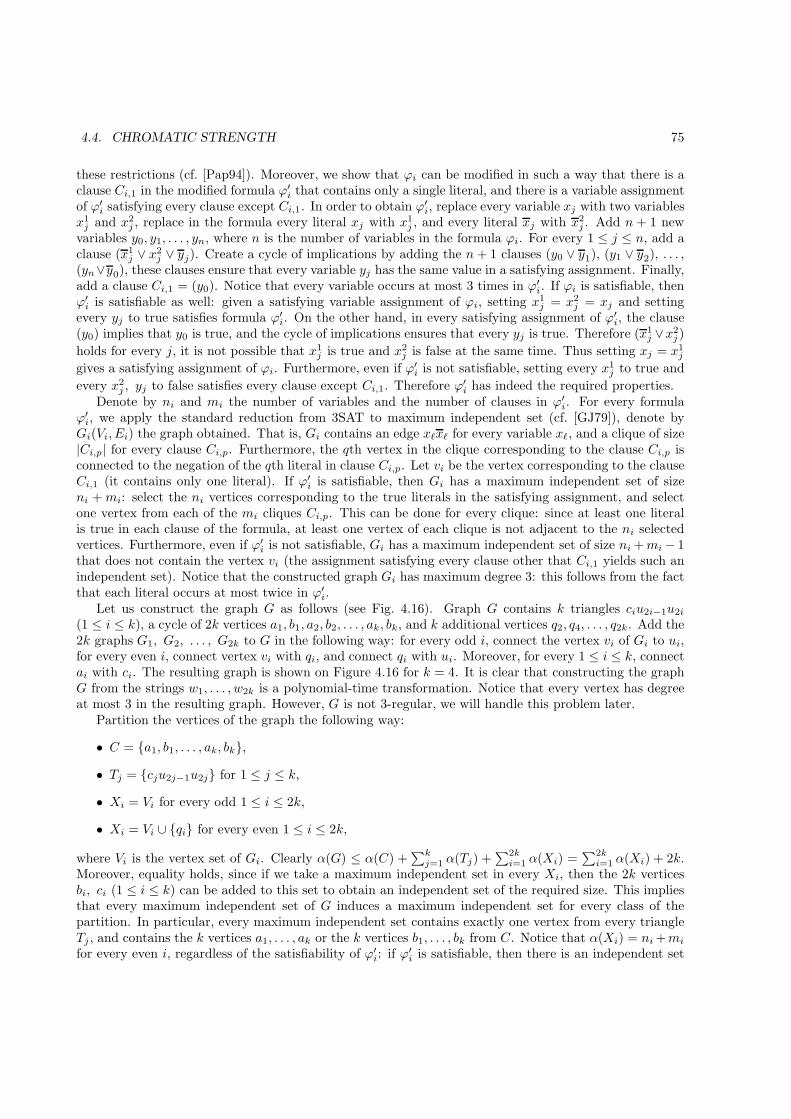
4.4. CHROMATIC STRENGTH 75
these restrictions (cf. [Pap94]). Moreover, we show that ϕi can be modified in such a way that there is aclause Ci,1 in the modified formula ϕ′
i that contains only a single literal, and there is a variable assignmentof ϕ′
i satisfying every clause except Ci,1. In order to obtain ϕ′i, replace every variable xj with two variables
x1j and x2
j , replace in the formula every literal xj with x1j , and every literal xj with x2
j . Add n + 1 newvariables y0, y1, . . . , yn, where n is the number of variables in the formula ϕi. For every 1 ≤ j ≤ n, add aclause (x1
j ∨ x2j ∨ yj). Create a cycle of implications by adding the n+ 1 clauses (y0 ∨ y1), (y1 ∨ y2), . . . ,
(yn∨y0), these clauses ensure that every variable yj has the same value in a satisfying assignment. Finally,add a clause Ci,1 = (y0). Notice that every variable occurs at most 3 times in ϕ′
i. If ϕi is satisfiable, thenϕ′i is satisfiable as well: given a satisfying variable assignment of ϕi, setting x1
j = x2j = xj and setting
every yj to true satisfies formula ϕ′i. On the other hand, in every satisfying assignment of ϕ′
i, the clause(y0) implies that y0 is true, and the cycle of implications ensures that every yj is true. Therefore (x1
j ∨x2j )
holds for every j, it is not possible that x1j is true and x2
j is false at the same time. Thus setting xj = x1j
gives a satisfying assignment of ϕi. Furthermore, even if ϕ′i is not satisfiable, setting every x1
j to true and
every x2j , yj to false satisfies every clause except Ci,1. Therefore ϕ′
i has indeed the required properties.Denote by ni and mi the number of variables and the number of clauses in ϕ′
i. For every formulaϕ′i, we apply the standard reduction from 3SAT to maximum independent set (cf. [GJ79]), denote byGi(Vi, Ei) the graph obtained. That is, Gi contains an edge xℓxℓ for every variable xℓ, and a clique of size|Ci,p| for every clause Ci,p. Furthermore, the qth vertex in the clique corresponding to the clause Ci,p isconnected to the negation of the qth literal in clause Ci,p. Let vi be the vertex corresponding to the clauseCi,1 (it contains only one literal). If ϕ′
i is satisfiable, then Gi has a maximum independent set of sizeni + mi: select the ni vertices corresponding to the true literals in the satisfying assignment, and selectone vertex from each of the mi cliques Ci,p. This can be done for every clique: since at least one literalis true in each clause of the formula, at least one vertex of each clique is not adjacent to the ni selectedvertices. Furthermore, even if ϕ′
i is not satisfiable, Gi has a maximum independent set of size ni +mi− 1that does not contain the vertex vi (the assignment satisfying every clause other that Ci,1 yields such anindependent set). Notice that the constructed graph Gi has maximum degree 3: this follows from the factthat each literal occurs at most twice in ϕ′
i.Let us construct the graph G as follows (see Fig. 4.16). Graph G contains k triangles ciu2i−1u2i
(1 ≤ i ≤ k), a cycle of 2k vertices a1, b1, a2, b2, . . . , ak, bk, and k additional vertices q2, q4, . . . , q2k. Add the2k graphs G1, G2, . . . , G2k to G in the following way: for every odd i, connect the vertex vi of Gi to ui,for every even i, connect vertex vi with qi, and connect qi with ui. Moreover, for every 1 ≤ i ≤ k, connectai with ci. The resulting graph is shown on Figure 4.16 for k = 4. It is clear that constructing the graphG from the strings w1, . . . , w2k is a polynomial-time transformation. Notice that every vertex has degreeat most 3 in the resulting graph. However, G is not 3-regular, we will handle this problem later.
Partition the vertices of the graph the following way:
• C = {a1, b1, . . . , ak, bk},
• Tj = {cju2j−1u2j} for 1 ≤ j ≤ k,
• Xi = Vi for every odd 1 ≤ i ≤ 2k,
• Xi = Vi ∪ {qi} for every even 1 ≤ i ≤ 2k,
where Vi is the vertex set of Gi. Clearly α(G) ≤ α(C) +∑k
j=1 α(Tj) +∑2ki=1 α(Xi) =
∑2ki=1 α(Xi) + 2k.
Moreover, equality holds, since if we take a maximum independent set in every Xi, then the 2k verticesbi, ci (1 ≤ i ≤ k) can be added to this set to obtain an independent set of the required size. This impliesthat every maximum independent set of G induces a maximum independent set for every class of thepartition. In particular, every maximum independent set contains exactly one vertex from every triangleTj , and contains the k vertices a1, . . . , ak or the k vertices b1, . . . , bk from C. Notice that α(Xi) = ni+mi
for every even i, regardless of the satisfiability of ϕ′i: if ϕ′
i is satisfiable, then there is an independent set
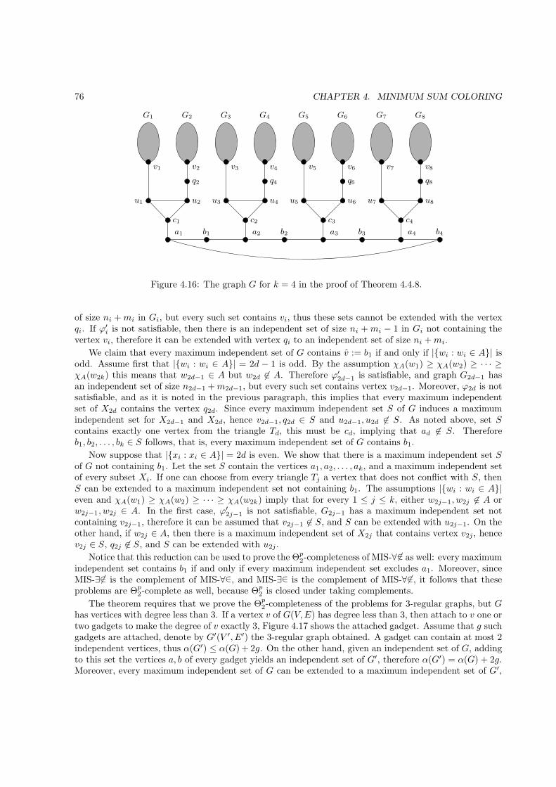
76 CHAPTER 4. MINIMUM SUM COLORING
G1
v3 v4 v5 v6 v7 v8
b4a4
q8
u8u7
b3a3
u6
q6
u5
b2
q4
u4u3
a2a1
v1
u1
v2
q2
u2
b1
G2 G3 G4 G5 G6 G7 G8
c1 c2 c3 c4
Figure 4.16: The graph G for k = 4 in the proof of Theorem 4.4.8.
of size ni + mi in Gi, but every such set contains vi, thus these sets cannot be extended with the vertexqi. If ϕ′
i is not satisfiable, then there is an independent set of size ni + mi − 1 in Gi not containing thevertex vi, therefore it can be extended with vertex qi to an independent set of size ni +mi.
We claim that every maximum independent set of G contains v := b1 if and only if |{wi : wi ∈ A}| isodd. Assume first that |{wi : wi ∈ A}| = 2d − 1 is odd. By the assumption χA(w1) ≥ χA(w2) ≥ · · · ≥χA(w2k) this means that w2d−1 ∈ A but w2d 6∈ A. Therefore ϕ′
2d−1 is satisfiable, and graph G2d−1 hasan independent set of size n2d−1 +m2d−1, but every such set contains vertex v2d−1. Moreover, ϕ2d is notsatisfiable, and as it is noted in the previous paragraph, this implies that every maximum independentset of X2d contains the vertex q2d. Since every maximum independent set S of G induces a maximumindependent set for X2d−1 and X2d, hence v2d−1, q2d ∈ S and u2d−1, u2d 6∈ S. As noted above, set Scontains exactly one vertex from the triangle Td, this must be cd, implying that ad 6∈ S. Thereforeb1, b2, . . . , bk ∈ S follows, that is, every maximum independent set of G contains b1.
Now suppose that |{xi : xi ∈ A}| = 2d is even. We show that there is a maximum independent set Sof G not containing b1. Let the set S contain the vertices a1, a2, . . . , ak, and a maximum independent setof every subset Xi. If one can choose from every triangle Tj a vertex that does not conflict with S, thenS can be extended to a maximum independent set not containing b1. The assumptions |{wi : wi ∈ A}|even and χA(w1) ≥ χA(w2) ≥ · · · ≥ χA(w2k) imply that for every 1 ≤ j ≤ k, either w2j−1, w2j 6∈ A orw2j−1, w2j ∈ A. In the first case, ϕ′
2j−1 is not satisfiable, G2j−1 has a maximum independent set notcontaining v2j−1, therefore it can be assumed that v2j−1 6∈ S, and S can be extended with u2j−1. On theother hand, if w2j ∈ A, then there is a maximum independent set of X2j that contains vertex v2j , hencev2j ∈ S, q2j 6∈ S, and S can be extended with u2j.
Notice that this reduction can be used to prove the Θp2-completeness of MIS-∀6∈ as well: every maximum
independent set contains b1 if and only if every maximum independent set excludes a1. Moreover, sinceMIS-∃6∈ is the complement of MIS-∀∈, and MIS-∃∈ is the complement of MIS-∀6∈, it follows that theseproblems are Θp
2-complete as well, because Θp2 is closed under taking complements.
The theorem requires that we prove the Θp2-completeness of the problems for 3-regular graphs, but G
has vertices with degree less than 3. If a vertex v of G(V,E) has degree less than 3, then attach to v one ortwo gadgets to make the degree of v exactly 3, Figure 4.17 shows the attached gadget. Assume that g suchgadgets are attached, denote by G′(V ′, E′) the 3-regular graph obtained. A gadget can contain at most 2independent vertices, thus α(G′) ≤ α(G) + 2g. On the other hand, given an independent set of G, addingto this set the vertices a, b of every gadget yields an independent set of G′, therefore α(G′) = α(G) + 2g.Moreover, every maximum independent set of G can be extended to a maximum independent set of G′,
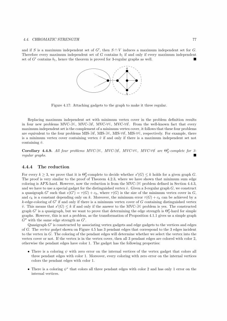
4.4. CHROMATIC STRENGTH 77
and if S is a maximum independent set of G′, then S ∩ V induces a maximum independent set for G.Therefore every maximum independent set of G contains b1 if and only if every maximum independentset of G′ contains b1, hence the theorem is proved for 3-regular graphs as well. �
a
b
Figure 4.17: Attaching gadgets to the graph to make it three regular.
Replacing maximum independent set with minimum vertex cover in the problem definition resultsin four new problems MVC-∃∈, MVC-∃6∈, MVC-∀∈, MVC-∀6∈. From the well-known fact that everymaximum independent set is the complement of a minimum vertex cover, it follows that these four problemsare equivalent to the four problems MIS-∃6∈, MIS-∃∈, MIS-∀6∈, MIS-∀∈, respectively. For example, thereis a minimum vertex cover containing vertex v if and only if there is a maximum independent set notcontaining v.
Corollary 4.4.9. All four problems MVC-∃∈, MVC-∃6∈, MVC-∀∈, MVC-∀6∈ are Θp2-complete for 3-
regular graphs. �
4.4.4 The reduction
For every k ≥ 3, we prove that it is Θp2-complete to decide whether s′(G) ≤ k holds for a given graph G.
The proof is very similar to the proof of Theorem 4.2.3, where we have shown that minimum sum edgecoloring is APX-hard. However, now the reduction is from the MVC-∃∈ problem defined in Section 4.4.3,and we have to use a special gadget for the distinguished vertex v. Given a 3-regular graph G, we constructa quasigraph G′ such that ǫ(G′) = τ(G) + ck, where τ(G) is the size of the minimum vertex cover in G,and ck is a constant depending only on k. Moreover, the minimum error τ(G) + ck can be achieved by ak-edge-coloring of G′ if and only if there is a minimum vertex cover of G containing distinguished vertexv. This means that s′(G) ≤ k if and only if the answer to the MVC-∃∈ problem is yes. The constructedgraph G′ is a quasigraph, but we want to prove that determining the edge strength is Θp
2-hard for simplegraphs. However, this is not a problem, as the transformation of Proposition 4.1.1 gives us a simple graphG′′ with the same edge strength as G′.
Quasigraph G′ is constructed by associating vertex gadgets and edge gadgets to the vertices and edgesof G. The vertex gadget shown on Figure 4.5 has 3 pendant edges that correspond to the 3 edges incidentto the vertex in G. The coloring of the pendant edges will determine whether we select the vertex into thevertex cover or not. If the vertex is in the vertex cover, then all 3 pendant edges are colored with color 2,otherwise the pendant edges have color 1. The gadget has the following properties:
• There is a coloring ψ with zero error on the internal vertices of the vertex gadget that colors allthree pendant edges with color 1. Moreover, every coloring with zero error on the internal verticescolors the pendant edges with color 1.
• There is a coloring ψ∗ that colors all three pendant edges with color 2 and has only 1 error on theinternal vertices.
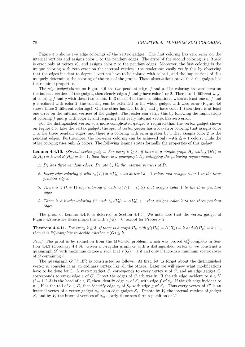
78 CHAPTER 4. MINIMUM SUM COLORING
Figure 4.5 shows two edge colorings of the vertex gadget. The first coloring has zero error on theinternal vertices and assigns color 1 to the pendant edges. The error of the second coloring is 1 (thereis error only at vertex v), and assigns color 2 to the pendant edges. Moreover, the first coloring is theunique coloring with zero error on the internal vertices: the reader can easily verify this by observingthat the edges incident to degree 1 vertices have to be colored with color 1, and the implications of thisuniquely determines the coloring of the rest of the graph. These observations prove that the gadget hasthe required properties.
The edge gadget shown on Figure 4.6 has two pendant edges f and g. If a coloring has zero error onthe internal vertices of the gadget, then clearly edges f and g have color 1 or 2. There are 4 different waysof coloring f and g with these two colors. In 3 out of 4 of these combinations, when at least one of f andg is colored with color 2, the coloring can be extended to the whole gadget with zero error (Figure 4.6shows these 3 different colorings). On the other hand, if both f and g have color 1, then there is at leastone error on the internal vertices of the gadget. The reader can verify this by following the implicationsof coloring f and g with color 1, and requiring that every internal vertex has zero error.
For the distinguished vertex v, a more complicated gadget is required than the vertex gadget shownon Figure 4.5. Like the vertex gadget, the special vertex gadget has a low-error coloring that assigns color1 to the three pendant edges, and there is a coloring with error greater by 1 that assigns color 2 to thependant edges. Furthermore, the low-error coloring can be achieved only with ∆ + 1 colors, while theother coloring uses only ∆ colors. The following lemma states formally the properties of this gadget:
Lemma 4.4.10. (Special vertex gadget) For every k ≥ 3, if there is a simple graph Hk with χ′(Hk) =∆(Hk) = k and s′(Hk) = k + 1, then there is a quasigraph Dk satisfying the following requirements:
1. Dk has three pendant edges. Denote by V0 the internal vertices of D.
2. Every edge coloring ψ with ǫψ(V0) = ǫ(V0) uses at least k + 1 colors and assigns color 1 to the threependant edges.
3. There is a (k + 1)-edge-coloring ψ with ǫψ(V0) = ǫ(V0) that assigns color 1 to the three pendantedges.
4. There is a k-edge-coloring ψ∗ with ǫψ∗(V0) = ǫ(V0) + 1 that assigns color 2 to the three pendantedges.
The proof of Lemma 4.4.10 is deferred to Section 4.4.5. We note here that the vertex gadget ofFigure 4.5 satisfies these properties with ǫ(V0) = 0, except for Property 2.
Theorem 4.4.11. For every k ≥ 3, if there is a graph Hk with χ′(Hk) = ∆(Hk) = k and s′(Hk) = k+ 1,then it is Θp
2-complete to decide whether s′(G) ≤ k.
Proof. The proof is by reduction from the MVC-∃∈ problem, which was proved Θp2-complete in Sec-
tion 4.4.3 (Corollary 4.4.9). Given a 3-regular graph G with a distinguished vertex v, we construct aquasigraph G′ with maximum degree k such that s′(G) = k if and only if there is a minimum vertex coverof G containing v.
The quasigraph G′(V ′, E′) is constructed as follows. At first, let us forget about the distinguishedvertex v, consider it as an ordinary vertex like all the others. Later we will show what modificationshave to be done for v. A vertex gadget Sv corresponds to every vertex v of G, and an edge gadget Secorresponds to every edge e of G. Direct the edges of G arbitrarily. If the ith edge incident to v ∈ V(i = 1, 2, 3) is the head of e ∈ E, then identify edge ei of Sv with edge f of Se. If the ith edge incident tov ∈ V is the tail of e ∈ E, then identify edge ei of Sv with edge g of Se. Thus every vertex of G′ is aninternal vertex of a vertex gadget Sv or an edge gadget Se. Denote by Vv the internal vertices of gadgetSv and by Ve the internal vertices of Se, clearly these sets form a partition of V ′.
4.4. CHROMATIC STRENGTH 79
We claim that G′ has an edge coloring with error t if and only if G has a vertex cover with size t.Assume first that D ⊆ V is a vertex cover of G. If v ∈ D, then color gadget Sv using coloring ψ∗: everypendant edge has color 2 and there is 1 error on the internal vertices. If v 6∈ D, then we use coloring ψ ofthe vertex gadget: every pendant edge of Sv has color 1 and there is no error on the internal vertices. Nowconsider a gadget Se for some e ∈ E. The two pendant edges f and g are already colored with color 1 or2. However, at least one of them is colored with 2, since at least one end vertex of e is in D. Therefore,using one of the three colorings shown on Figure 4.6, we can extend the coloring to every edge of Se withzero error on the internal vertices of the gadget. Therefore errors appear only on the internal vertices ofSv for v ∈ D, and the total error of the coloring is |D|.
On the other hand, consider an edge coloring of G′ with error t. Let V ⊆ V be the set of those v ∈ Vfor which there is error in Vv. Similarly, let E ⊆ E be the set of those e ∈ E for which there is error in Ve.Clearly, the coloring has error at least |V | + |E| ≤ t. Let V be a set of |E| vertices in G that cover every
edge in E. The set of vertices V ∪ V has size at most |V | + |E| ≤ t. We show that this set is a vertex
cover of G. It is clear that every edge e ∈ E is covered, since there is a v ∈ V covering e. Now consider anedge e 6∈ E, this means that Ve is colored with zero error, thus, as we have observed, at least one pendantedge of Se is colored with color 2. If this edge is the pendant edge of the vertex gadget Sv, then thereis at least one error in Vv and v is in V . However, if the pendant edge of Se and Sv is identified in theconstruction, this means that e is incident to v, thus v ∈ V covers e.
We have shown that ǫ(G′) = τ(G). Now we modify slightly G′ to take into account the distinguishedvertex v. The gadget corresponding to vertex v is not the vertex gadget of Figure 4.5, but the specialvertex gadget defined in Lemma 4.4.10. By modifying appropriately the argument presented above, onecan show that ǫ(G′) = τ(G) + ǫ(V0), where ǫ(V0) is the minimum error on the internal vertices of thespecial gadget. Moreover, if G has a minimum vertex cover D containing v, then G′ has a minimum sumedge coloring using only k colors, since in this case we can use coloring ψ∗ on the special gadget. On theother hand, if there is a minimum sum edge coloring using k colors, then by Property 2 of Lemma 4.4.10,the error is more than ǫ(V0) on the internal vertices of the special gadget. This means that vertex v is
contained in the set V defined above, hence the constructed minimum vertex cover contains v. Therefores′(G′) = k if and only if G has a minimum vertex cover containing v, what we had to prove. �
In Section 4.4.2 we have seen that for every k ≥ 3, there is a simple graph with maximum degree andchromatic index k that has edge strength k + 1. Combining this with Theorem 4.4.11 gives
Corollary 4.4.12. For every k ≥ 3, it is Θp2-complete to decide whether s′(G) ≤ k. �
Determining the chromatic edge strength is the special case of determining the chromatic strength:edge strength is simply the strength of the line graph. Therefore Corollary 4.4.12 implies hardness for thechromatic strength as well:
Corollary 4.4.13. For every k ≥ 3, it is Θp2-complete to decide whether s(G) ≤ k. �
In the introduction, we have noted that if G is a simple graph, then s′(G) is either ∆(G) or ∆(G) + 1[MMS97, HMT00], and consequently, s′(G) is either χ′(G) or χ′(G) + 1. In Theorem 4.4.11, we constructa graph with maximum degree and chromatic index k. Therefore comparing s′(G) to ∆(G) or to χ′(G) isalso hard:
Corollary 4.4.14. For every k ≥ 3, it is Θp2-complete to decide for graphs with maximum degree k whether
s′(G) = ∆(G) holds. �
Corollary 4.4.15. For every k ≥ 3, it is Θp2-complete to decide for graphs with maximum degree k whether
s′(G) = χ′(G) holds. �
Hajiabolhassan et al. [HMT00] asks an open question to characterize those graphs where s′(G) 6= χ′(G).Corollary 4.4.15 implies that we cannot hope for a nontrivial (NP or coNP) characterization of such graphs.

80 CHAPTER 4. MINIMUM SUM COLORING
T4T3T2
432e e e e
T1
2 2
22 2
2
1
1
1 1
1 1
1
11
1
1
1
1 1
1
r r r
r r r r
N3N2N1
3
3
Figure 4.18: The trees Ti and Ni.
4.4.5 Special vertex gadget
The aim of this section is to construct the special vertex gadget defined in Lemma 4.4.10. However,some preparations are required before the proof. We recursively construct two families of trees Ti and Ni(i ≥ 1). Every Ti has a pendant edge e, and every Ni has a root r. The trees T1 and N1 consist of a singleedge. The tree Ni is constructed by attaching the pendant edges of a T1, T2, . . . , Ti tree to a common rootr. The tree Ti+1 is the same as Ni, with a pendant edge connected to the root r. The construction isdemonstrated on Figure 4.18.
The properties of these trees are summarized in the following lemma:
Lemma 4.4.16. (a) There is an edge coloring of the tree Ti that has no error on the internal vertices ofTi, and assigns color i to the pendant edge e. Furthermore, every coloring that assigns color j to e haserror at least |j − i| on the internal vertices.(b) There is a zero error edge coloring of the tree Ni that assigns the colors 1, 2, . . . , i to the edges incidentto r. Furthermore, if color j ≤ i is missing at r in a coloring, then this coloring has error at least i− j+ 1on the internal vertices of Ni.
Proof. The proof is by induction on i. Both statements are trivial for i = 1. Now assume that i > 1 andboth (a) and (b) hold for every 1 ≤ j < i. First we prove statement (a). Since Ti − e is an Ni−1 tree,thus it has a zero error coloring by the induction hypotheses. Extending this coloring by assigning colori to edge e does not create errors on the internal vertices of Ti, proving the first part of statement (a).Consider now an edge coloring that assigns color j to e. This coloring colors Ti − e = Ni−1 in such a waythat color j is missing from vertex r. If j < i, then by the induction hypothesis, there is error at least(i − 1) − j + 1 = |j − i| on the internal vertices of Ni−1, and we are ready. On the other hand, if j > i,then in the coloring of Ti the degree i internal vertex r has error at least j − i.
Next we prove statement (b). Let e1, e2, . . . , ei be the edges incident to r in Ni, edge ej is the pendantedge of the Tj tree attached to r. A zero error edge coloring of Ni can be obtained by coloring everyattached tree Tj in such a way that the internal vertices have zero error and edge ej has color j. Clearly,there is no error on r on any other vertex of Ni in this coloring.
Suppose that a color j ≤ i is missing from r in a coloring ψ of Ni. Define the following sequence ofedges: es1 = ej and esk+1
= eψ(esk) until an edge with ψ(esk′
) > i is found (it can be verified that this
sequence is finite). Since eskis the pendant edge of a tree Tsk
, by statement (a), there is error at least|sk − ψ(esk
)| on the internal vertices of Tsk. Therefore the internal vertices of Ni has error at least
|ψ(es1) − s1| + |ψ(es2) − s2| + · · · + |ψ(esk′−1
) − sk′−1| + |ψ(esk′) − sk′ |
≥ (ψ(es1) − s1) + (ψ(es2) − s2) + · · · + (ψ(esk′−1
) − sk′−1) + (ψ(esk′) − sk′)
= ψ(esk′) − s1 ≥ i+ 1 − j
since by definition, ψ(esk) = sk+1 for 1 ≤ k < k′, and ψ(esk′
) > i. �
4.4. CHROMATIC STRENGTH 81
The colorings defined by Lemma 4.4.16 will be called the standard colorings of these gadgets.Denote by Σ′
∆(G) the minimum sum that a ∆(G)-edge-coloring of G can have, clearly Σ′∆(G) ≥ Σ′(G).
Denote by ǫ∆(G) the error of the best ∆(G)-edge-coloring, that is, ǫ∆(G) = 2Σ′∆(G) − ℓ(G).
In the following lemma, we determine how the error on the vertices changes if we attach to vertex vof G1 an edge of G2.
Lemma 4.4.17. Let G1(V1, E1) and G2(V2, E2) be two graphs such that V1 ∩ V2 = {v} and edge e is theonly edge in G2 incident to v. Let d be the degree of v in G1. Let G(V1∪V2, E1∪E2) be the graph obtainedby joining G1 and G2 at vertex v. If ψ1 is an edge coloring of G1, ψ2 is an edge coloring of G2, and thesecolorings assign distinct colors to the edges incident to v, then they can be combined to obtain an edgecoloring ψ of G such that
ǫψ(u) =
ǫψ1(u) if u ∈ V1 \ {v}
ǫψ2(u) if u ∈ V2 \ {v}
ǫψ1(u) + ψ2(e) − (d+ 1) if u = v.
Conversely, if ψ is an edge coloring of G, then it induces an edge coloring ψ1 of G1 such that
ǫψ1(u) =
{ǫψ(u) if u ∈ V1 \ {v}
ǫψ(v) − ψ(e) + d+ 1 if u = v.
Proof. The first statement clearly holds for every vertex u 6= v, since combining the two colorings canchange the error only on v, the only common vertex of the two graphs. Let Ev ⊆ E1 be the edges incidentto v in G1. The error of v in coloring ψ is
ǫψ(v) = Σ′ψ(v) −
d+1∑
i=1
i =∑
f∈Ev
ψ(f) + ψ(e) −d∑
i=1
i− (d+ 1)
=
∑
f∈Ev
ψ1(f) −d∑
i=1
i
+ ψ2(e) − (d+ 1) = ǫψ1(v) + ψ2(e) − (d+ 1).
The second statement can be proved by a similar calculation. �
In particular, if we attach a tree Td(v) to a vertex v, then the error changes as follows:
Lemma 4.4.18. Let v be an arbitrary vertex of simple graph G(V,E), attach to v the pendant edge e ofthe tree Td(v). Denote by G′ the graph obtained.
(a) The error ǫ(G′) is either ǫ(G)− 1 or ǫ(G) + 1, and it is ǫ(G)− 1 if and only if there is a minimumsum edge coloring ψ of G such that some color c ≤ d(v) is missing from v.
(b) If d(v) < ∆(G), then ǫ∆(G′) is either ǫ∆(G) − 1 or ǫ∆(G) + 1, and it is ǫ∆(G) − 1 if and only ifthere is a ∆(G)-edge-coloring with error ǫ∆(G) where some color c′ ≤ d(v) is missing from v.
Proof. Let ψ be a minimum sum edge coloring of G, and let c ≤ d(v) + 1 be the smallest color not presentat v in ψ. Take the standard coloring of Td(v) that has zero error on the internal vertices and assigns colord(v) to edge e (Lemma 4.4.16a). Exchange in Td(v) the colors d(v) and c on the alternating path startingat edge e, this results in a coloring of Td(v) that has |d(v)− c| error the internal vertices and assigns colorc to edge e. This coloring can be combined with ψ to obtain a coloring ψ′ of G′. We use Lemma 4.4.17to calculate the error of ψ′. The total error on the internal vertices of Td(v) is |d(v) − c|, and the error onthe vertices of G is the same as in ψ, except on v, where the error is increased by c− (d(v) + 1). Thereforethe error of ψ′ is ǫψ′(G′) = ǫψ(G) + c− (d(v) + 1) + |d(v)− c|. If c ≤ d(v), then this equals ǫψ(G)− 1, thus
82 CHAPTER 4. MINIMUM SUM COLORING
ǫ(G′) ≤ ǫ(G) − 1. If c = d(v) + 1, then ǫψ′(G) = ǫψ(G) + 1, and ǫ(G′) ≤ ǫ(G) + 1 follows. Therefore wehave obtained that ǫ(G′) ≤ ǫ(G) + 1, and if G has a minimum sum edge coloring where a color c ≤ d(v)is missing from v, then ǫ(G′) ≤ ǫ(G) − 1.
To finish the proof of statement (a), we have to show that ǫ(G′) ≥ ǫ(G) − 1, and if every minimumsum edge coloring of G uses at v every color not greater than d(v), then ǫ(G′) ≥ ǫ(G) + 1. Assume that aminimum sum coloring ψ′ of G′ is given with ψ′(e) = c. By Lemma 4.4.16 there is error at least |d(v)− c|on the internal vertices of the tree Td(v), so there is error at most ǫ(G′) − |d(v) − c| on the vertices V .Coloring ψ′ induces a coloring ψ of G, and by the second part of Lemma 4.4.17,
ǫψ(G) = ǫψ′(V ) − c+ d(v) + 1 ≤ ǫ(G′) − |d(v) − c| − c+ d(v) + 1 ≤ ǫ(G′) + 1,
hence ǫ(G′) ≥ ǫψ(G) − 1 ≥ ǫ(G) − 1. Moreover, equality is only possible if c ≤ d(v) and ψ is a minimumsum edge coloring of G, or in other words, if there is a minimum sum edge coloring of G such that colorc ≤ d(v) is missing from v. Finally, if every minimum sum coloring of G uses every color not greater thand(v) on v, then either c > d(v) or ψ is not a minimum sum coloring of G. In either case, ǫψ′(G′) ≥ ǫ(G)+1follows, completing the proof of statement (a) (recall that if ψ is not a minimum sum coloring of G, thenǫψ(G) ≥ ǫ(G) + 2, since the error of every coloring has the same parity). The proof of statement (b) isexactly the same. Notice that if d(v) < ∆(G), then ∆(G′) = ∆(G). �
The following gadget will be used in the construction of the special vertex gadget.
Lemma 4.4.19. For every k ≥ 1, there is a quasigraph Hk satisfying the following properties (V0 denotesthe internal vertices of Hk):
1. H has two pendant edges f, g.
2. There is a (k + 1)-edge-coloring ψk+1 with ψk+1(f) = k + 1, ψk+1(g) = 1 and ǫψk+1(V0) = 0.
3. For every i ≤ k, there is a (k + 1)-edge-coloring ψi with ψi(f) = i, ψi(g) = 2, and ǫψi(V0) = k − i.
4. For every coloring ψ, if ψ(f) = i ≤ k, then ǫψ(V0) ≥ k − i.
5. For every coloring ψ, if ψ(f) = k + 1 and ǫψ(V0) = 0, then ψ(g) = 1.
Proof. For k = 1, 2, 3, the graph Hk is shown on Figure 4.19. It can be verified directly that they satisfythe requirements of the lemma. Henceforth it is assumed that k ≥ 4.
The graph Hk is constructed as follows. Take a path of 6 vertices v1, v2, v3, v4, v5, v6, let f = v1v2 andg = v5v6. Identify the root of a tree Nk−1 with vertex v2. Attach a half-loop to v3, and attach to v3the pendant edges of k − 2 trees T2, T3, . . . , Tk−1. Attach a half-loop to v4 as well, and attach to v4 thependant edges of k − 3 trees T3, T4, . . . , Tk−1. The resulting graph Hk is demonstrated on Figure 4.19.
The coloring ψk+1 is defined as ψk+1(v1v2) = k+ 1, ψk+1(v2v3) = k, ψk+1(v3v4) = 1, ψk+1(v4v5) = 2,ψk+1(v5v6) = 1, ψk+1(v3v3) = k + 1, ψk+1(v4v4) = k, and it gives the standard coloring to the attachedtrees. It can be verified that ψk+1 is a proper edge coloring and there is zero error on the internalvertices, which gives Property 2. Similarly, the coloring ψk required by Property 3 for i = k is defined asψk(v1v2) = k, ψk(v2v3) = k + 1, ψk(v3v4) = k, ψk(v4v5) = 1, ψk(v5v6) = 2, ψk(v3v3) = 1, ψk(v4v4) = 2.
To obtain the coloring ψi for some i < k (Property 3), take the coloring ψk defined above, and exchangethe colors k and i on the alternating path starting from edge f . This introduces error k − i to only onevertex, namely to the vertex at the other end of the alternating path. Notice that this color exchangecannot affect edge g, since edge v2v3 has color k+ 1. Therefore we obtain a coloring satisfying Property 3.
To see that Property 4 holds, observe that a coloring ψ of Hk induces a coloring of the tree Nk−1, andcolor ψ(f) is missing from the root of Nk−1. Therefore in this coloring of Nk−1, there is error at leastk − 1 − ψ(f) + 1 = k − i on the internal vertices (Lemma 4.4.16b), and this means that ψ has error atleast k − i on the internal vertices of Hk, as required.
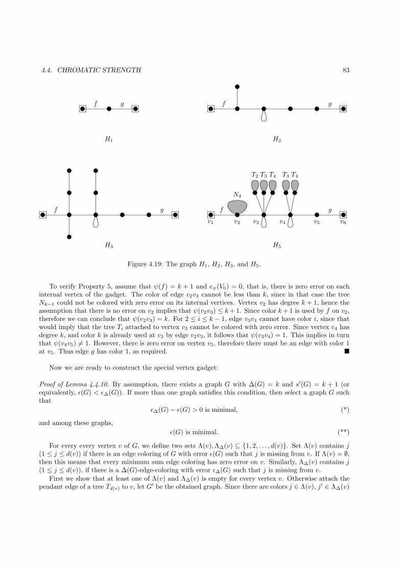
4.4. CHROMATIC STRENGTH 83
v2v1 v5 v6v3 v4
N4
T2 T4T4T3 T3
H5H3
H2H1
f f
f f
g g
g g
Figure 4.19: The graph H1, H2, H3, and H5.
To verify Property 5, assume that ψ(f) = k + 1 and eψ(V0) = 0, that is, there is zero error on eachinternal vertex of the gadget. The color of edge v2v3 cannot be less than k, since in that case the treeNk−1 could not be colored with zero error on its internal vertices. Vertex v2 has degree k + 1, hence theassumption that there is no error on v2 implies that ψ(v2v3) ≤ k+ 1. Since color k+ 1 is used by f on v2,therefore we can conclude that ψ(v2v3) = k. For 2 ≤ i ≤ k − 1, edge v3v4 cannot have color i, since thatwould imply that the tree Ti attached to vertex v3 cannot be colored with zero error. Since vertex v4 hasdegree k, and color k is already used at v3 by edge v2v3, it follows that ψ(v3v4) = 1. This implies in turnthat ψ(v4v5) 6= 1. However, there is zero error on vertex v5, therefore there must be an edge with color 1at v5. Thus edge g has color 1, as required. �
Now we are ready to construct the special vertex gadget:
Proof of Lemma 4.4.10. By assumption, there exists a graph G with ∆(G) = k and s′(G) = k + 1 (orequivalently, ǫ(G) < ǫ∆(G)). If more than one graph satisfies this condition, then select a graph G suchthat
ǫ∆(G) − ǫ(G) > 0 is minimal, (*)
and among these graphs,
ǫ(G) is minimal. (**)
For every every vertex v of G, we define two sets Λ(v),Λ∆(v) ⊆ {1, 2, . . . , d(v)}. Set Λ(v) contains j(1 ≤ j ≤ d(v)) if there is an edge coloring of G with error ǫ(G) such that j is missing from v. If Λ(v) = ∅,then this means that every minimum sum edge coloring has zero error on v. Similarly, Λ∆(v) contains j(1 ≤ j ≤ d(v)), if there is a ∆(G)-edge-coloring with error ǫ∆(G) such that j is missing from v.
First we show that at least one of Λ(v) and Λ∆(v) is empty for every vertex v. Otherwise attach thependant edge of a tree Td(v) to v, let G′ be the obtained graph. Since there are colors j ∈ Λ(v), j′ ∈ Λ∆(v)
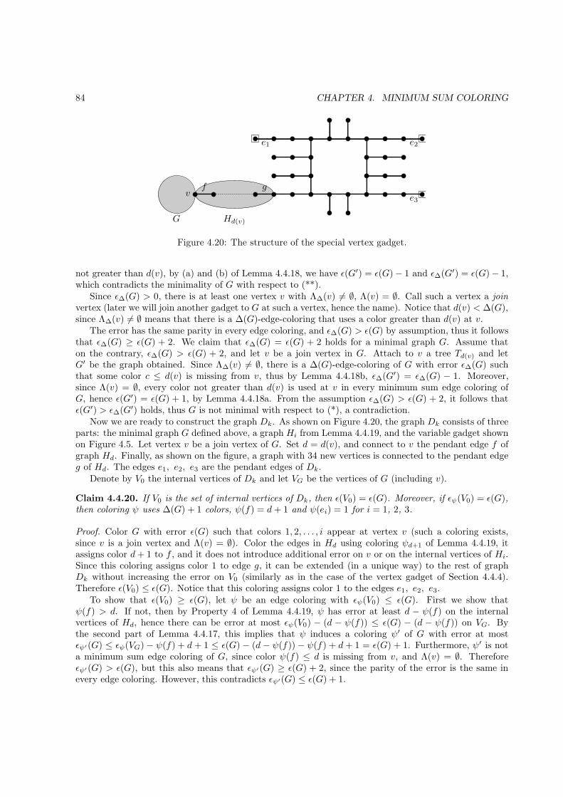
84 CHAPTER 4. MINIMUM SUM COLORING
v
G
e1 e2
e3
Hd(v)
f g
Figure 4.20: The structure of the special vertex gadget.
not greater than d(v), by (a) and (b) of Lemma 4.4.18, we have ǫ(G′) = ǫ(G) − 1 and ǫ∆(G′) = ǫ(G) − 1,which contradicts the minimality of G with respect to (**).
Since ǫ∆(G) > 0, there is at least one vertex v with Λ∆(v) 6= ∅, Λ(v) = ∅. Call such a vertex a joinvertex (later we will join another gadget to G at such a vertex, hence the name). Notice that d(v) < ∆(G),since Λ∆(v) 6= ∅ means that there is a ∆(G)-edge-coloring that uses a color greater than d(v) at v.
The error has the same parity in every edge coloring, and ǫ∆(G) > ǫ(G) by assumption, thus it followsthat ǫ∆(G) ≥ ǫ(G) + 2. We claim that ǫ∆(G) = ǫ(G) + 2 holds for a minimal graph G. Assume thaton the contrary, ǫ∆(G) > ǫ(G) + 2, and let v be a join vertex in G. Attach to v a tree Td(v) and letG′ be the graph obtained. Since Λ∆(v) 6= ∅, there is a ∆(G)-edge-coloring of G with error ǫ∆(G) suchthat some color c ≤ d(v) is missing from v, thus by Lemma 4.4.18b, ǫ∆(G′) = ǫ∆(G) − 1. Moreover,since Λ(v) = ∅, every color not greater than d(v) is used at v in every minimum sum edge coloring ofG, hence ǫ(G′) = ǫ(G) + 1, by Lemma 4.4.18a. From the assumption ǫ∆(G) > ǫ(G) + 2, it follows thatǫ(G′) > ǫ∆(G′) holds, thus G is not minimal with respect to (*), a contradiction.
Now we are ready to construct the graph Dk. As shown on Figure 4.20, the graph Dk consists of threeparts: the minimal graph G defined above, a graph Hi from Lemma 4.4.19, and the variable gadget shownon Figure 4.5. Let vertex v be a join vertex of G. Set d = d(v), and connect to v the pendant edge f ofgraph Hd. Finally, as shown on the figure, a graph with 34 new vertices is connected to the pendant edgeg of Hd. The edges e1, e2, e3 are the pendant edges of Dk.
Denote by V0 the internal vertices of Dk and let VG be the vertices of G (including v).
Claim 4.4.20. If V0 is the set of internal vertices of Dk, then ǫ(V0) = ǫ(G). Moreover, if ǫψ(V0) = ǫ(G),then coloring ψ uses ∆(G) + 1 colors, ψ(f) = d+ 1 and ψ(ei) = 1 for i = 1, 2, 3.
Proof. Color G with error ǫ(G) such that colors 1, 2, . . . , i appear at vertex v (such a coloring exists,since v is a join vertex and Λ(v) = ∅). Color the edges in Hd using coloring ψd+1 of Lemma 4.4.19, itassigns color d+ 1 to f , and it does not introduce additional error on v or on the internal vertices of Hi.Since this coloring assigns color 1 to edge g, it can be extended (in a unique way) to the rest of graphDk without increasing the error on V0 (similarly as in the case of the vertex gadget of Section 4.4.4).Therefore ǫ(V0) ≤ ǫ(G). Notice that this coloring assigns color 1 to the edges e1, e2, e3.
To show that ǫ(V0) ≥ ǫ(G), let ψ be an edge coloring with ǫψ(V0) ≤ ǫ(G). First we show thatψ(f) > d. If not, then by Property 4 of Lemma 4.4.19, ψ has error at least d − ψ(f) on the internalvertices of Hd, hence there can be error at most ǫψ(V0) − (d − ψ(f)) ≤ ǫ(G) − (d − ψ(f)) on VG. Bythe second part of Lemma 4.4.17, this implies that ψ induces a coloring ψ′ of G with error at mostǫψ′(G) ≤ ǫψ(VG) − ψ(f) + d + 1 ≤ ǫ(G) − (d − ψ(f)) − ψ(f) + d + 1 = ǫ(G) + 1. Furthermore, ψ′ is nota minimum sum edge coloring of G, since color ψ(f) ≤ d is missing from v, and Λ(v) = ∅. Thereforeǫψ′(G) > ǫ(G), but this also means that ǫψ′(G) ≥ ǫ(G) + 2, since the parity of the error is the same inevery edge coloring. However, this contradicts ǫψ′(G) ≤ ǫ(G) + 1.

4.4. CHROMATIC STRENGTH 85
Therefore it can be assumed that ψ(f) > d for any coloring with ǫψ(V0) ≤ ǫ(G). Now, again byLemma 4.4.17, ψ induces a coloring ψ′ of G with error ǫψ′(G) = ǫψ(VG) − ψ(f) + (d + 1) ≤ ǫψ(VG) ≤ǫψ(V0) ≤ ǫ(G). Since ǫψ′(G) ≥ ǫ(G), there have to be inequalities throughout. In particular, ψ(f) = d+ 1and ǫψ(V0) = ǫ(G), thus ǫ(V0) cannot be strictly smaller than ǫ(G). Furthermore, every coloring ψ withǫψ(V0) = ǫ(G) induces a coloring ψ′ of G with error ǫ(G). We know that error ǫ(G) can be achieved onlyby using ∆(G) + 1 colors. Therefore ∆(G) + 1 colors are required to achieve error ǫ(V0) = ǫ(G) on V0.Moreover, we have seen that in such a coloring ψ, there is color d + 1 on f and the error on V0 \ V iszero. By Property 5 of Lemma 4.4.19, this implies that ψ(g) = 1 and it follows that the pendant edgese1, e2, e3 also have color 1, as required. �
Property 2 of the Lemma follows immediately from Claim 4.4.20. Moreover, in the proof we haveconstructed a coloring ψ with ǫψ(V0) = ǫ(V0) and ψ(ei) = 1 for i = 1, 2, 3, which implies Property 3.
To show that Property 4 holds, color G using ∆(G) colors with error ǫ∆(G) = ǫ(G) + 2 such that colorc ∈ Λ∆(v) is missing from vertex v, denote by ψ∆ this coloring. Color Hd such that edge f has color d,edge g has color 2, and there is error d−c on the internal vertices of Hd (the coloring ψc from Property 3 ofLemma 4.4.19). This coloring can be extended to a coloring of Dk without introducing further errors on V0
(see the second coloring on Figure 4.5), which gives a coloring ψ∗ that assigns color 2 to the three pendantedges e1, e2, e3. We use the first part of Lemma 4.4.17 to determine ǫψ∗(V0). There is error d−c on V0\V ,and ǫψ∗(u) = ǫψ∆(u) for every u ∈ V \ {v}. By Lemma 4.4.17, ǫψ∗(v) = ǫψ∆(v) + ψ∗(f) − (d(v) + 1) =ǫψ∆(G) + c−d−1. Therefore ǫψ∗(V0) = ǫψ∆(G) + (c−d−1) + (d− c) = ǫ∆(G)−1 = ǫ(G) + 1 = ǫ(V0) + 1,as required. �

CHAPTER 5
Minimum sum multicoloring
There are not more than five primary colors (blue, yellow, red, white, and black),yet in combination they produce more hues than can ever been seen.
Sun Tzu (circa 500 B.C.), The Art Of War
In Chapter 4 we have seen that minimum sum coloring can be used to model the scheduling of dependentjobs if the goal is to minimize the sum of completion times. However, we have assumed that every jobrequires a unit amount of time, exactly one time slot has to be assigned to each job. In this chapter wegeneralize minimum sum coloring in such a way that it can model different time requirements.
In the minimum sum multicoloring problem a graph G(V,E) is given with a demand x(v) for eachvertex. In the scheduling application, this demand will correspond to the number of time slots the jobrequires. The colors are the positive integers, they correspond to the time slots. We have to assign a setof x(v) colors to each vertex v such that neighbors receive disjoint sets of colors. Given a coloring, thecompletion time of a job will be the largest color assigned to the vertex of the job. Thus it is not importantwhat is the color set assigned to a vertex, only the largest color of this color set counts. Therefore tominimize the sum of completion times, we have to minimize the sum of these largest colors. Formally, theproblem is defined as follows:
Minimum Sum Multicoloring
Input: A graph G(V,E) and a demand function x: V → N.
Output: A multicoloring Ψ: V → 2N such that
• |Ψ(v)| = x(v) for every v ∈ V , and
• Ψ(u) ∩ Ψ(v) = ∅ if u and v are neighbors in G.
Goal: Let the finish time of vertex v in coloring Ψ be the highest color assigned to it, fΨ(v) =max{i : i ∈ Ψ(v)}. The goal is to minimize
∑v∈V fΨ(v), the sum of the coloring Ψ.
There are two variants of the problem. In the preemptive version the color set Ψ(v) can be arbitrary. Inthe non-preemptive version we require that Ψ(v) contains a consecutive set of colors. This latter variantcan be used to model non-preemptive scheduling problems, where it is not allowed to interrupt a job

88 CHAPTER 5. MINIMUM SUM MULTICOLORING
once it is started. Such non-preemptive problems can arise when we schedule jobs on machines and itis physically impossible (or very expensive) to stop a job and continue it later. On the other hand, ina computer or network setting it is quite common to preempt a task and continue it later, usually thiscan be done with only a small overhead. The preemptive and non-preemptive versions of a schedulingproblem can be very different. In a preemptive problem we have to assign a set of time slots to eachjob, while in the non-preemptive problem a single number (the starting time or the completion time)is sufficient. Therefore in the non-preemptive problems the search space is usually smaller, which canmake exact solution easier. On the other hand, in a preemptive problem we have more tools to modify asolution, which can be useful when designing approximation algorithms. In this chapter we consider onlythe preemptive version of minimum sum multicoloring. If a set Ψ(v) is assigned to v, then the number ofpreemptions in Ψ(v) is the number of different i’s such that i ≤ fΨ(v), i 6∈ Ψ(v), but i− 1 ∈ Ψ(v). If Ψ(v)is a continuous interval, then it has zero preemptions; if it is the union of two intervals, then it has onepreemption, etc.
Minimum sum multicoloring was introduced in [BNHK+99, BNHK+00]. The problem is hard, andit is hard even to approximate: the best known polynomial-time algorithm has approximation ratioO(n/ log2 n) [BNHK+00]. The same paper gives a 16-approximation algorithm for perfect graphs and a7.184-approximation for interval graphs. However, very recently a 5.436-approximation was found for per-fect graphs, which improves both results. For bipartite graphs [BNHK+00] gives a 1.5-approximation algo-rithm. For trees a polynomial time approximation scheme (PTAS) is given by Halldorsson et al. [HKP+03],which was later generalized for partial k-trees and planar graphs [HK02].
In [HKP+03] a PTAS is given for the minimum sum multicoloring of trees, but no hardness resultwas proved for the problem. It was asked as an open question what is the complexity of minimum summulticoloring on trees, and if it is NP-hard, then whether it is possible to solve the problem in polynomialtime for paths. We answer the first question in Section 5.2 by showing that the problem is NP-hard forbinary trees. Kovacs [Kov04] gave a partial answer to the second question by showing that minimum summulticoloring can be solved in O(n3p) time for a path of length n if the maximum demand is p. Thisalgorithm is only pseudopolynomial, since the maximum demand can be exponentially large. As of thiswriting, it is still an open question whether there is a polynomial time algorithm for the problem on paths.In Section 5.1 we prove a structural result that might help resolving this question. We show that for pathsthere is always an optimum solution where every color set is the union of O(log p) continuous intervals.For bipartite graphs and perfect graphs, we prove the weaker bounds O(n) and O(n2), respectively, onthe number of preemptions required per vertex in an optimum solution.
In Section 5.3 and Section 5.4 we investigate the edge coloring version of minimum sum multicoloring,which can be formulated as follows:
Minimum Sum Edge Multicoloring
Input: A graph G(V,E) and a demand function x: E → N.
Output: A multicoloring Ψ: E → 2N such that
• |Ψ(e)| = x(e) for every edge e, and
• Ψ(e1) ∩ Ψ(e2) = ∅ if e1 and e2 are adjacent in G.
Goal: The finish time of edge e in coloring Ψ is the highest color assigned to it, fΨ(e) =max{c : c ∈ Ψ(e)}. The goal is to minimize fΨ(G) =
∑e∈E fΨ(e), the sum of the coloring Ψ.
An application of edge coloring is to model dedicated scheduling of biprocessor tasks. The verticescorrespond to the processors and each edge e = uv corresponds to a job that requires x(e) time units ofsimultaneous work on the two preassigned processors u and v. The colors correspond to the available timeslots: by assigning x(e) colors to edge e, we select the x(e) time units when the job corresponding to e is
5.1. NUMBER OF PREEMPTIONS 89
executed. A processor cannot work on two jobs at the same time, this corresponds to the requirement thata color can appear at most once on the edges incident to a vertex. The finish time of edge e correspondsto the time slot when job e is completed, therefore minimizing the sum of the finish times is the same asminimizing the sum of completion times of the jobs. Such biprocessor tasks arise when we want to schedulefile transfers between processors [CGJL85] or the mutual diagnostic testing of processors [HvdVV94]. Notethat it is allowed that a job is interrupted and continued later: the set of colors assigned to an edge doesnot have to be consecutive, hence our problem models preemptive scheduling.
Of particular interest is the case where the graph to be colored is bipartite. A possible application ofthe bipartite problem is the following. One bipartition class corresponds to a set of clients, the other classcorresponds to a set of servers. An edge e between two vertices means that the given client has to accessthe given server for x(e) units of time. A client can access only one server at the same time, and a servercannot accept connections from more than one client simultaneously. Clearly, bipartite edge multicoloringmodels this situation.
Minimum sum edge multicoloring is a generalization of minimum sum edge coloring, hence any com-plexity result for the latter problem also applies to the multicoloring version as well. Furthermore, inSection 5.3 we show that although minimum sum edge coloring is polynomial-time solvable for trees[GK00, Sal03], the multicoloring version is NP-hard, even if every demand is 1 or 2. On the other hand,we also show that the problem is polynomial time solvable for trees if every demand is the same. Thisis a consequence of the following scaling property of minimum sum edge multicoloring in trees (provedin Section 5.4.2): if the demand of every edge is multiplied by the same integer q, then the sum of theoptimum solution increases by a factor of q.
In Section 5.4 we give a polynomial time approximation scheme (PTAS) for minimum sum edgemulticoloring of trees. Before that, the 2-approximation algorithm of [BNHK+00] for arbitrary graphswas the only known approximation result for minimum sum edge multicoloring.
The material of Section 5.2 is taken from [Mar02]; Section 5.3 and Section 5.4 appeared as [Mar04g,Mar04h].
5.1 Number of preemptions
The main result of this section is the following. Consider an instance of minimum sum multicoloring on apath. Let p be the maximum demand in the graph, p = maxv∈V x(v). We show that there is a minimumsum multicoloring with at most O(log p) preemptions at every vertex. Such a structural result might beuseful when designing algorithms for the problem.
Besides possible algorithmic applications, there is another reason for trying to bound the number ofpreemptions required by the optimum solutions. If x(v) appears in binary form in the input, then p can beexponentially large. Now it is not at all trivial that the decision version of the problem (is there a coloringwith sum at most C?) is in NP, since it is not obvious how an optimum solution could be described inpolynomial length. Our result shows that for paths the problem is indeed in NP: the optimum solutioncan be compactly represented by describing O(log p) intervals for each vertex. Moreover, we also showthat if the graph is perfect and has n vertices, then there is always an optimum solution with at mostn2 preemptions at every vertex, regardless of the size of p. Thus the optimum solution can be given asn · n2 intervals, hence the problem is in NP for perfect graphs. The proof uses polyhedral arguments. Ifthe graph is bipartite, then simple observations show that there is an optimum solution with at most npreemptions.
Notation and basic observations are given in Section 5.1.1. Section 5.1.2 defines several operations,which will be used to transform colorings. Section 5.1.3 proves a key structural property of optimumcolorings. In Section 5.1.4, this observation is used to bound the number of preemptions required in anoptimum coloring. Section 5.1.5 investigates more general classes of graphs and bounds the number ofpreemptions required in bipartite and perfect graphs.
90 CHAPTER 5. MINIMUM SUM MULTICOLORING
5.1.1 Preliminaries
We slightly extend the problem by allowing x(v) = 0. It is clear that this does not change the problem,but it will be useful for technical reasons. If x(v) = 0 then let fΨ(v) = 0 in every coloring Ψ. Note thatby using this definition the trivial inequality fΨ(v) ≥ x(v) holds even if x(v) = 0.
We introduce some notational conventions. Let fΨ(V ′) =∑
v∈V ′ fΨ(v) for any V ′ ⊆ V and coloringΨ. Similarly, x(V ′) =
∑v∈V ′ x(v). If x(v) = 1, then we will write Ψ(v) = a instead of Ψ(v) = {a}. We
denote the sum of the optimal coloring of G with demand function x by OPT(G, x), or by OPT(G) if thefunction x(v) is clear from the context. The set [a, b] is the set of integers {a, a+ 1, . . . , b}. A node v iscompact in coloring Ψ if fΨ(v) = x(v).
We define a secondary objective function, which is to maximize∑v∈V f
2Ψ(v). Call a coloring Ψ square-
optimal if its sum is minimum, and among such colorings,∑
v∈V f2Ψ(v) is maximum. Note that in an
optimum solution the secondary objective function can be bounded by n ·OPT 2(G).In this section we will always assume that G is a path. Let 1, 2 , . . . , n be the nodes of G along
the path in left to right order. For convenience, we set x(0) = x(n + 1) = fΨ(0) = fΨ(n + 1) = 0 inevery coloring Ψ. Node v is a local maximum in Ψ if fΨ(v) > fΨ(v − 1) and fΨ(v) > fΨ(v + 1), andit is a local minimum if fΨ(v) < fΨ(v − 1) and fΨ(v) < fΨ(v + 1). Node v is an upward step in Ψ iffΨ(v − 1) < fΨ(v) < fΨ(v + 1) and it is a downward step if fΨ(v − 1) > fΨ(v) > fΨ(v + 1).
In [HK02] it is proved that every optimum coloring uses at most O(p · χ(G) · logn) (where p is themaximum demand) colors, for bipartite graphs, this is O(p · logn). It is easy to see that in an optimumcoloring of a path fΨ(i) ≤ 3p holds for every i: the neighbors Ψ(i− 1) and Ψ(i + 1) forbid the use of atmost 2p colors and x(i) ≤ p.
Proposition 5.1.1. If Ψ is an optimum coloring of a path, then fΨ(i) ≤ 3p. �
A coloring Ψ is a conflicting coloring if |Ψ(v)| = x(v) is satisfied for every node v, but Ψ(u)∩Ψ(v) = ∅does not hold for some neighbors u and v. A conflicting coloring contains one or more conflicts, where aconflict is a triple (u, v, c) such that u and v are neighboring nodes and c ∈ Ψ(u), c ∈ Ψ(v). In a path, aconflict is of the form (v, v + 1, c).
5.1.2 Operations
In this section we define several operations that transform a coloring to another one. These transformationswill be used in Section 5.1.3 and 5.1.4 to show certain properties of optimum colorings. Before presentingthe transformations, let us have a note about the figures. In the figures to follow, the horizontal axiscorresponds to the path, and the vertical axis corresponds to the set of colors. The black parts of thecolumns show which colors are assigned to the given node. For example, on Figure 5.1, node v has twointervals of consecutive colors between color a and b.
The parity shift operation from u to v in the range a to b transforms a coloring Ψ to a coloring Φ asfollows. Let Φ(w) = Ψ(w) for all w < u and w > v (see Figure 5.1). Otherwise let x′(w) = |Ψ(w) ∩ [a, b]|and
Φ(w) =
{(Ψ(w) ∩ [1, a− 1]) ∪ (Ψ(w) ∩ [b+ 1,∞]) ∪ [a, a+ x′(w) − 1] if w ≡ u (mod 2)(Ψ(w) ∩ [1, a− 1]) ∪ (Ψ(w) ∩ [b+ 1,∞]) ∪ [b− x′(w) + 1, b] if w 6≡ u (mod 2)
Clearly, |Φ(w)| = x(w), but Φ is not, in general, a proper coloring, there might be conflicts betweenu and u − 1, and between v and v + 1. However, if fΨ(u − 1) < a < b and fΨ(v + 1) < a < b, then Φis a proper coloring. The operation can increase the finish time for only those vertices w that has paritydifferent from u. But if the finish time is greater than b for all such w between u and v, then their finishtime is not increased, hence the sum of Φ is not greater than the sum of Ψ.
The second operation is the change of colors a and b from u to v, resulting in a new coloring Φ. Itdoes not change the colors assigned to nodes w < u and w > v, and for every node u ≤ w ≤ v and
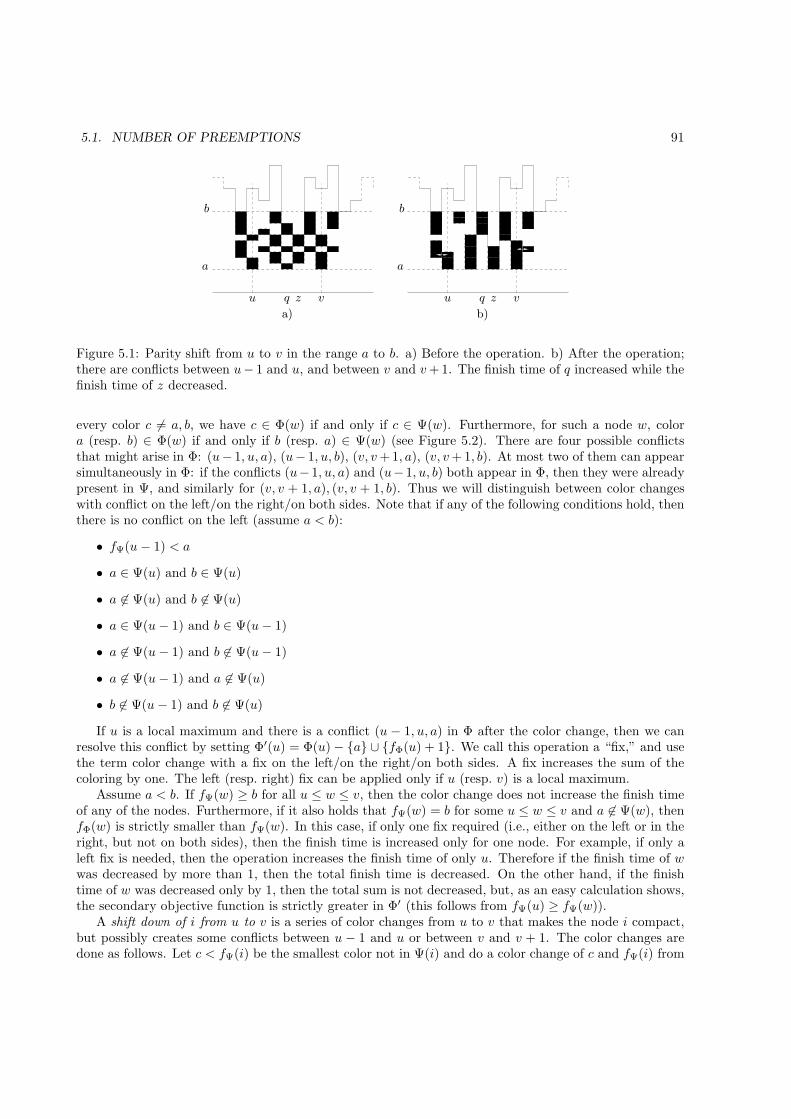
5.1. NUMBER OF PREEMPTIONS 91
q qz z
b b
a a
v vu u
b)a)
Figure 5.1: Parity shift from u to v in the range a to b. a) Before the operation. b) After the operation;there are conflicts between u− 1 and u, and between v and v+ 1. The finish time of q increased while thefinish time of z decreased.
every color c 6= a, b, we have c ∈ Φ(w) if and only if c ∈ Ψ(w). Furthermore, for such a node w, colora (resp. b) ∈ Φ(w) if and only if b (resp. a) ∈ Ψ(w) (see Figure 5.2). There are four possible conflictsthat might arise in Φ: (u− 1, u, a), (u− 1, u, b), (v, v+ 1, a), (v, v+ 1, b). At most two of them can appearsimultaneously in Φ: if the conflicts (u−1, u, a) and (u−1, u, b) both appear in Φ, then they were alreadypresent in Ψ, and similarly for (v, v + 1, a), (v, v + 1, b). Thus we will distinguish between color changeswith conflict on the left/on the right/on both sides. Note that if any of the following conditions hold, thenthere is no conflict on the left (assume a < b):
• fΨ(u − 1) < a
• a ∈ Ψ(u) and b ∈ Ψ(u)
• a 6∈ Ψ(u) and b 6∈ Ψ(u)
• a ∈ Ψ(u− 1) and b ∈ Ψ(u− 1)
• a 6∈ Ψ(u− 1) and b 6∈ Ψ(u− 1)
• a 6∈ Ψ(u− 1) and a 6∈ Ψ(u)
• b 6∈ Ψ(u− 1) and b 6∈ Ψ(u)
If u is a local maximum and there is a conflict (u − 1, u, a) in Φ after the color change, then we canresolve this conflict by setting Φ′(u) = Φ(u) − {a} ∪ {fΦ(u) + 1}. We call this operation a “fix,” and usethe term color change with a fix on the left/on the right/on both sides. A fix increases the sum of thecoloring by one. The left (resp. right) fix can be applied only if u (resp. v) is a local maximum.
Assume a < b. If fΨ(w) ≥ b for all u ≤ w ≤ v, then the color change does not increase the finish timeof any of the nodes. Furthermore, if it also holds that fΨ(w) = b for some u ≤ w ≤ v and a 6∈ Ψ(w), thenfΦ(w) is strictly smaller than fΨ(w). In this case, if only one fix required (i.e., either on the left or in theright, but not on both sides), then the finish time is increased only for one node. For example, if only aleft fix is needed, then the operation increases the finish time of only u. Therefore if the finish time of wwas decreased by more than 1, then the total finish time is decreased. On the other hand, if the finishtime of w was decreased only by 1, then the total sum is not decreased, but, as an easy calculation shows,the secondary objective function is strictly greater in Φ′ (this follows from fΨ(u) ≥ fΨ(w)).
A shift down of i from u to v is a series of color changes from u to v that makes the node i compact,but possibly creates some conflicts between u − 1 and u or between v and v + 1. The color changes aredone as follows. Let c < fΨ(i) be the smallest color not in Ψ(i) and do a color change of c and fΨ(i) from
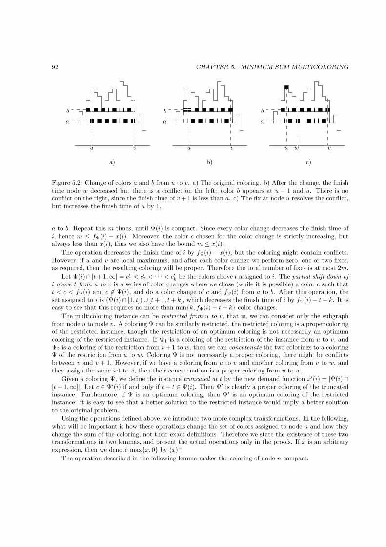
92 CHAPTER 5. MINIMUM SUM MULTICOLORING
\
w
b bb
a aa
u u uv v v
c)a) b)
Figure 5.2: Change of colors a and b from u to v. a) The original coloring. b) After the change, the finishtime node w decreased but there is a conflict on the left: color b appears at u − 1 and u. There is noconflict on the right, since the finish time of v+ 1 is less than a. c) The fix at node u resolves the conflict,but increases the finish time of u by 1.
a to b. Repeat this m times, until Ψ(i) is compact. Since every color change decreases the finish time ofi, hence m ≤ fΨ(i) − x(i). Moreover, the color c chosen for the color change is strictly increasing, butalways less than x(i), thus we also have the bound m ≤ x(i).
The operation decreases the finish time of i by fΨ(i) − x(i), but the coloring might contain conflicts.However, if u and v are local maximums, and after each color change we perform zero, one or two fixes,as required, then the resulting coloring will be proper. Therefore the total number of fixes is at most 2m.
Let Ψ(i)∩ [t+ 1,∞] = c′1 < c′2 < · · · < c′k be the colors above t assigned to i. The partial shift down ofi above t from u to v is a series of color changes where we chose (while it is possible) a color c such thatt < c < fΨ(i) and c 6∈ Ψ(i), and do a color change of c and fΨ(i) from a to b. After this operation, theset assigned to i is (Ψ(i) ∩ [1, t])∪ [t+ 1, t+ k], which decreases the finish time of i by fΨ(i) − t− k. It iseasy to see that this requires no more than min{k, fΨ(i) − t− k} color changes.
The multicoloring instance can be restricted from u to v, that is, we can consider only the subgraphfrom node u to node v. A coloring Ψ can be similarly restricted, the restricted coloring is a proper coloringof the restricted instance, though the restriction of an optimum coloring is not necessarily an optimumcoloring of the restricted instance. If Ψ1 is a coloring of the restriction of the instance from u to v, andΨ2 is a coloring of the restriction from v+ 1 to w, then we can concatenate the two colorings to a coloringΨ of the restriction from u to w. Coloring Ψ is not necessarily a proper coloring, there might be conflictsbetween v and v + 1. However, if we have a coloring from u to v and another coloring from v to w, andthey assign the same set to v, then their concatenation is a proper coloring from u to w.
Given a coloring Ψ, we define the instance truncated at t by the new demand function x′(i) = |Ψ(i) ∩[t+ 1,∞]|. Let c ∈ Ψ′(i) if and only if c+ t ∈ Ψ(i). Then Ψ′ is clearly a proper coloring of the truncatedinstance. Furthermore, if Ψ is an optimum coloring, then Ψ′ is an optimum coloring of the restrictedinstance: it is easy to see that a better solution to the restricted instance would imply a better solutionto the original problem.
Using the operations defined above, we introduce two more complex transformations. In the following,what will be important is how these operations change the set of colors assigned to node n and how theychange the sum of the coloring, not their exact definitions. Therefore we state the existence of these twotransformations in two lemmas, and present the actual operations only in the proofs. If x is an arbitraryexpression, then we denote max{x, 0} by (x)+.
The operation described in the following lemma makes the coloring of node n compact:
5.1. NUMBER OF PREEMPTIONS 93
Lemma 5.1.2. For every coloring Ψ there is a coloring Φ such that Φ(n) = [1, x(n)] and fΦ(V ) ≤fΨ(V ) + (fΨ(n) − fΨ(n− 1))+.
Proof. We consider three cases: (1) fΨ(n) < fΨ(n− 1), (2) fΨ(n− 2) < fΨ(n− 1) < fΨ(n), (3) fΨ(n) >fΨ(n− 1) and fΨ(n− 1) < fΨ(n− 2).
In the first case, let u be the first local maximum to the left of n. It exists because fΨ(0) = x(0) = 0.We do a shift down of n from u to n. This consists of a series of at most fΨ(n)−x(n) color changes, eachof them requires at most one fix, since there is no conflict on the right. The finish time of n is decreasedby fΨ(n) − x(n), thus the total sum is not increased.
In the second case, let s = |Ψ(n − 1) ∩ [1, x(n)]| ≤ fΨ(n) − x(n). The new coloring Φ is the same asΨ except Φ(n) = [1, x(n)] and Φ(n− 1) = (Ψ(n− 1) ∩ [x(n) + 1,∞]) ∪ [fΨ(n) + 1, fΨ(n) + s]. It is easilyverified that this is a proper coloring. The finish time of n is decreased by fΨ(n) − x(n) and the finishtime of n− 1 is increased to fΨ(n) + s, that is, by at most fΨ(n) + fΨ(n) − x(n) − fΨ(n− 1). Thus thetotal increase is at most fΨ(n) − fΨ(n− 1).
In the third case, we let u be the first local maximum to the left of n − 1 and do a shift down of nfrom u to n. This requires at most fΨ(n)− x(n) left fixes, and increases the finish time of n− 1 to fΨ(n),that is, by at most fΨ(n) − fΨ(n− 1). Since the finish time of n is decreased by fΨ(n) − x(n), the totalincrease of the sum is at most fΨ(n) − fΨ(n− 1), what we had to prove. �
The second operation also makes node n compact. However, here we assume that the color set [1, α]is already assigned to n.
Lemma 5.1.3. Assume that Ψ is a coloring and for some α, we have [1, α] ⊆ Ψ(n) and |Ψ(n)∩[α+1,∞]| =β. Then there is a coloring Φ such that Φ(n) = [1, x(n)] and fΦ(V ) ≤ fΨ(V )+β+(fΨ(n)−fΨ(n−1))+ +x(n) − fΨ(n).
Proof. We consider again the previous three cases: (1) fΨ(n) < fΨ(n− 1), (2) fΨ(n − 2) < fΨ(n − 1) <fΨ(n), (3) fΨ(n) > fΨ(n− 1) and fΨ(n− 1) < fΨ(n− 2).
In the first case, let u be the first local maximum to the left of n. We do a partial shift down of n fromu to n above α. This consists of a series of at most β color changes, each of them requires at most onefix, since there cannot be conflict on the right. The finish time of n is decreased by fΨ(n) − x(n), thusthe total increase of the sum is at most β + x(n) − fΨ(n).
In the second case, let s = |Ψ(n − 1) ∩ [α + 1, α + β]| ≤ β. The new coloring Φ is the same as Ψexcept that Φ(n) = [1, x(n)] and Φ(n− 1) = (Ψ(n− 1)∩ [x(n) + 1,∞])∪ [fΨ(n) + 1, fΨ(n) + s]. It is easilyverified that this is a proper coloring (note that α+ β = x(n) holds). The finish time of n is decreased byfΨ(n)−x(n) and the finish time of n−1 is increased to fΨ(n)+s, that is, by at most β+fΨ(n)−fΨ(n−1),thus we are ready with this case.
In the third case, we let u be the first local maximum to the left of n− 1 and do a partial shift downof n from u to n above α. This requires at most β left fixes, and increases the finish time of n− 1 by atmost fΨ(n) − fΨ(n− 1). Since the finish time of n is decreased by fΨ(n) − x(n), the total increase of thesum is at most β + (fΨ(n) − fΨ(n− 1)) + x(n) − fΨ(n), what we had to prove. �
We have seen in Prop. 5.1.1 that the finish time of a node can be bounded by a constant multiple ofthe maximum demand. The following lemma shows that if i is not a local maximum then its finish timecan be bounded in terms of its own demand.
Lemma 5.1.4. If Ψ is an optimum solution and i is not a local maximum, then fΨ(i) ≤ 4x(i).
Proof. Assume first that i is a local minimum, let u (resp. v) be the first local maximum to the left(resp. right) of i. If Ψ(i) is not compact, then we perform a shift down of i from u to v. This requires atmost x(i) color changes. Therefore the fixes increase the sum by at most 2x(i). However, the finish timeof i is decreased by fΨ(i) − x(i). Assuming that Ψ is an optimum coloring, it follows that fΨ(i) ≤ 3x(i).
94 CHAPTER 5. MINIMUM SUM MULTICOLORING
Now assume without loss of generality that i is an upward step. Denote by v the first local maximumto the right of i.
First we first modify the coloring Ψ to achieve that fΨ(i) − fΨ(i − 1) ≤ x(i). We do a partial shiftdown of i above fΨ(i − 1) from i to v. This series of color changes does not require any left fixes. Sinceevery color change decreases the finish time of i by at least one, this shift operation does not increase thetotal sum. After this operation, [fΨ′(i−1)+1, fΨ′(i)] ⊆ Ψ′(i) in the resulting coloring Ψ′, which obviouslyimplies f ′
Ψ(i) − f ′Ψ(i− 1) ≤ x(i). Thus in the following we can assume that fΨ(i) − fΨ(i− 1) ≤ x(i).
Now consider the restriction of the instance from 1 to i. We can apply Lemma 5.1.3 to node iwith α = 0 and β = x(i). Therefore there exists a coloring Φ1 with Φ1(i) = [1, x(i)] and fΦ1([1, i]) ≤fΨ([1, i]) + β + (fΨ(i) − fΨ(i− 1))+ + x(i) − fΨ(i) ≤ fΨ([1, i− 1]) + 3x(i).
Next we restrict the instance and the coloring Ψ from i to n, and do a shift down of i from i to v.This requires at most x(i) fixes on the right and no fixes on the left. The finish time of i is decreased byfΨ(i) − x(i), thus for the resulting coloring Φ2, we have fΦ2([i, n]) ≤ fΨ([i, n]) + x(i) + x(i) − fΨ(i). Wecan concatenate Φ1 and Φ2 to a coloring Φ of the original instance since they assign the same set to i.We can bound the sum of Φ by
fΦ([1, n]) = fΦ1([1, i]) + fΦ2([i, n]) − fΦ2(i) ≤
≤ (fΨ([1, i− 1]) + 3x(i)) + (fΨ([i, n]) + 2x(i) − fΨ(i)) − x(i) =
= fΨ([1, n]) + 4x(i) − fΨ(i)
By assumption, Ψ is an optimum coloring, thus the sum of Φ is not smaller than the sum of Ψ. By theinequalities shown above, this implies 4x(i) − fΨ(i) ≥ 0. �
5.1.3 Bounding the reduced sequence
Let ℓ(i)0 = i be the first element of the left sequence of the node i in a coloring Ψ, and for k ≥ 0 let ℓ
(i)k+1
be the largest j < ℓ(i)k such that fΨ(j) ≤ fΨ(ℓ
(i)k ) (see Figure 5.3). The last element of the sequence is
ℓ(i)L(i) = 0. The right sequence is similarly defined with r
(i)0 = i and r
(i)k+1 is the smallest j > r
(i)k such that
fΨ(j) ≤ fΨ(r(i)k ), the last element of the sequence is r
(i)R(i) = n+ 1. The reduced left (right) sequence is the
sequence truncated at the first compact node, its length is R′(i) (resp. L′(i)). The first compact node inthe sequence is included in the reduced sequence only if its finish time is greater than zero. In particular,if fΨ(i) = x(i) = 0, then L′(i) = R′(i) = 0.
In this section, our aim is to bound the length of the reduced left and right sequence of every node: inSection 5.1.4, Lemma 5.1.13 shows the connection between the length of these sequences and the numberof preemptions required in an optimum coloring. The following series of lemmas will prove that L′(i) isat most logarithmic in p. The bound for R′(i) follows by symmetry.
Lemma 5.1.5. If Ψ is a square-optimal solution, and nodes u and v are local minimums such that atleast one of them is not compact and for all u < w < v, we have fΨ(w) ≥ max{fΨ(u), fΨ(v)}, then u andv have opposite parity.
Proof. Let q be the first local maximum to the left of u and z the first local maximum to the right of v(see Figure 5.4). We do a shift down of u from q to u, with doing the required fixes on the left (but noton the right). This requires at most fΨ(u)− x(u) fixes and decreases the finish time of u by that amount,thus it does not increase the total sum. Similarly, we do a shift down of v from v to z (with doing fixeson the right), this does not increase the total sum either. There might be conflicts between u and u + 1or between v and v − 1, we resolve this by applying a parity shift from u to v in the range from 1 tomax{fΨ(u), fΨ(v)}. This does not change u and v, since they were already compact after the shift down,thus this results in a proper coloring. The parity shift does not increase the finish time of any of the nodesu < w < v, since, by assumption, they have finish time not smaller than max{fΨ(u), fΨ(v)}.
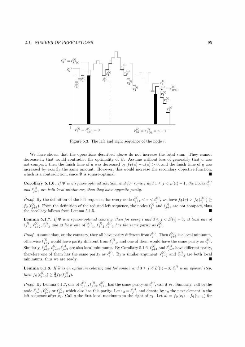
5.1. NUMBER OF PREEMPTIONS 95
i
r(i)10 = r
(i)
R(i) = n+ 1ℓ(i)7 = ℓ
(i)L(i) = 0
r(i)6 = r
(i)R′(i)
ℓ(i)3 = ℓ
(i)
L′(i)
ℓ(i)5
ℓ(i)6
ℓ(i)4
ℓ(i)1
r(i)9
r(i)8
r(i)7
r(i)5
r(i)4
r(i)3
r(i)2
r(i)1
ℓ(i)2
Figure 5.3: The left and right sequence of the node i.
We have shown that the operations described above do not increase the total sum. They cannotdecrease it, that would contradict the optimality of Ψ. Assume without loss of generality that u wasnot compact, then the finish time of u was decreased by fΨ(u) − x(u) > 0, and the finish time of q wasincreased by exactly the same amount. However, this would increase the secondary objective function,which is a contradiction, since Ψ is square-optimal. �
Corollary 5.1.6. If Ψ is a square-optimal solution, and for some i and 1 ≤ j < L′(i) − 1, the nodes ℓ(i)j
and ℓ(i)j+1 are both local minimums, then they have opposite parity.
Proof. By the definition of the left sequence, for every node ℓ(i)j+1 < v < ℓ
(i)j , we have fΨ(v) > fΨ(ℓ
(i)j ) ≥
fΨ(ℓ(i)j+1). From the definition of the reduced left sequence, the nodes ℓ
(i)j and ℓ
(i)j+1 are not compact, thus
the corollary follows from Lemma 5.1.5. �
Lemma 5.1.7. If Ψ is a square-optimal coloring, then for every i and 3 ≤ j < L′(i) − 3, at least one of
ℓ(i)j+1, ℓ
(i)j+2, ℓ
(i)j+3 and at least one of ℓ
(i)j−1, ℓ
(i)j−2, ℓ
(i)j−3 has the same parity as ℓ
(i)j .
Proof. Assume that, on the contrary, they all have parity different from ℓ(i)j . Then ℓ
(i)j+1 is a local minimum,
otherwise ℓ(i)j+2 would have parity different from ℓ
(i)j+1, and one of them would have the same parity as ℓ
(i)j .
Similarly, ℓ(i)j+2, ℓ
(i)j−2, ℓ
(i)j−3 are also local minimums. By Corollary 5.1.6, ℓ
(i)j+1 and ℓ
(i)j+2 have different parity,
therefore one of them has the same parity as ℓ(i)j . By a similar argument, ℓ
(i)j−2 and ℓ
(i)j−3 are both local
minimums, thus we are ready. �
Lemma 5.1.8. If Ψ is an optimum coloring and for some i and 3 ≤ j < L′(i)− 3, ℓ(i)j is an upward step,
then fΨ(ℓ(i)j−3) ≥ 9
8fΨ(ℓ(i)j+4).
Proof. By Lemma 5.1.7, one of ℓ(i)j+1, ℓ
(i)j+2, ℓ
(i)j+3 has the same parity as ℓ
(i)j , call it v1. Similarly, call v3 the
node ℓ(i)j−1, ℓ
(i)j−2 or ℓ
(i)j−3 which also has this parity. Let v2 = ℓ
(i)j , and denote by v0 the next element in the
left sequence after v1. Call q the first local maximum to the right of v3. Let di = fΨ(vi) − fΨ(vi−1) for
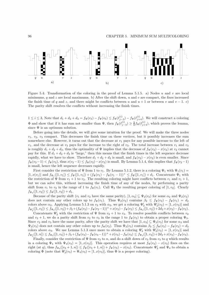
96 CHAPTER 5. MINIMUM SUM MULTICOLORING
replacemen
c)b)
q qq
a)
z z zv v vu u u
Figure 5.4: Transformation of the coloring in the proof of Lemma 5.1.5. a) Nodes u and v are localminimums, q and z are local maximums. b) After the shift down, u and v are compact, the fixes increasedthe finish time of q and z, and there might be conflicts between u and u + 1 or between v and v − 1. c)The parity shift resolves the conflicts without increasing the finish times.
1 ≤ i ≤ 3, Note that d1 + d2 + d3 = fΨ(v3) − fΨ(v0) ≤ fΨ(ℓ(i)j−3) − fΨ(ℓ
(i)j+4). We will construct a coloring
Φ and show that if it has sum not smaller than Ψ, then fΨ(ℓ(i)j−3) ≥ 9
8fΨ(ℓ(i)j+4), which proves the lemma,
since Ψ is an optimum solution.
Before going into the details, we will give some intuition for the proof. We will make the three nodesv1, v2, v3 compact. This decreases the finish time on these vertices, but it possibly increases the sumsomewhere else. However, it turns out that the decrease at v1 pays for any possible increase to the left ofv1, and the decrease at v3 pays for the increase to the right of v3. The total increase between v1 and v3is roughly d1 + d2 + d3, thus the optimality of Ψ implies that the decrease of fΨ(v2) − x(v2) at v2 cannotpay for this. If d1 + d2 + d3 is “large,” then this means that the finish times in the left sequence decreaserapidly, what we have to show. Therefore d1 + d2 + d3 is small, and fΨ(v2) − x(v2) is even smaller. SincefΨ(v2−1) < fΨ(v2), thus x(v2−1) ≤ fΨ(v2)−x(v2) is small. By Lemma 5.1.4, this implies that fΨ(v2−1)is small, hence the left sequence decreases rapidly.
First consider the restriction of Ψ from 1 to v1. By Lemma 5.1.2, there is a coloring Ψ1 with Ψ1(v1) =[1, x(v1)] and fΨ1([1, v1]) ≤ fΨ([1, v1]) + (fΨ(v1) − fΨ(v1 − 1))+ ≤ fΨ([1, v1]) + d1. Concatenate Ψ1 withthe restriction of Ψ from v1 + 1 to v2. The resulting coloring might have conflicts between v1 and v1 + 1,but we can solve this, without increasing the finish time of any of the nodes, by performing a parityshift from v1 to v2 in the range of 1 to fΨ(v1). Call Ψ2 the resulting proper coloring of [1, v2]. ClearlyfΨ2([1, v2]) ≤ fΨ([1, v2]) + d1.
Because of the parity shift (v1 and v2 have the same parity), [1, α2] ⊆ Ψ2(v2) for some α2 and Ψ2(v2)does not contain any other colors up to fΨ(v1). Thus Ψ2(v2) contains β2 ≤ fΨ(v2) − fΨ(v1) = d2
colors above α2. Applying Lemma 5.1.3 on v2 with α2, we get a coloring Ψ′2 with Ψ′
2(v2) = [1, x(v2)] andfΨ′
2([1, v2]) ≤ fΨ2([1, v2])+β2+(fΨ(v2)−fΨ(v2−1))++x(v2)−fΨ(v2) ≤ fΨ2([1, v2])+2d2+x(v2)−fΨ(v2).
Concatenate Ψ′2 with the restriction of Ψ from v2 + 1 to v3. To resolve possible conflicts between v2
and v2 + 1, we do a parity shift from v2 to v3 in the range 1 to fΨ(v2) to obtain a proper coloring Ψ3.Since v2 and v3 have the same parity, after the parity shift we have that [1, α3] ⊆ Ψ3(v3) for some α3 andΨ3(v3) does not contain any other colors up to fΨ(v2). Thus Ψ3(v3) contains β3 ≤ fΨ(v3) − fΨ(v2) = d3
colors above α3. We use Lemma 5.1.3 once more to obtain a coloring Ψ′3 with Ψ′
3(v3) = [1, x(v3)] andfΨ′
3([1, n]) ≤ fΨ3([1, v3])+β3+(fΨ(v3)−fΨ(v3−1))++x(v3)−fΨ(v3) ≤ fΨ3([1, v3])+2d3+x(v3)−fΨ(v3).
Finally, consider the restriction of Ψ from v3 to n, and do a shift down of v3 from v3 to q which resultsin a coloring Ψ4 with Ψ4(v3) = [1, x(v3)]. This operation requires at most fΨ(v3) − x(v3) fixes on theright (at q), thus fΨ4([v3 + 1, n]) ≤ fΨ([v3 + 1, n]) + fΨ(v3) − x(v3). Concatenate Ψ′
3 and Ψ4 to obtain acoloring Φ (note that Ψ′
3(v3) = Ψ4(v3) = [1, x(v3)], thus Φ is a proper coloring).

5.1. NUMBER OF PREEMPTIONS 97
Now we bound the sum of Φ using the inequalities obtained above:
fΦ([1, n]) = fΨ′
3([1, v3]) + fΨ4([v3 + 1, n]) ≤
≤ (fΨ3([1, v3]) + 2d3 + x(v3) − fΨ(v3)) + (fΨ([v3 + 1, n]) + fΨ(v3) − x(v3)) =
= fΨ′
2([1, v2]) + fΨ([v2 + 1, v3]) + 2d3 + fΨ([v3 + 1, n]) ≤
≤ fΨ2([1, v2]) + 2d2 + x(v2) − fΨ(v2) + 2d3 + fΨ([v2 + 1, n]) ≤
≤ fΨ([1, v2]) + d1 + 2d2 + x(v2) − fΨ(v2) + 2d3 + fΨ([v2 + 1, n]) ≤
≤ fΨ([1, n] + 2(d1 + d2 + d3) + x(v2) − fΨ(v2)
By assumption, Ψ is an optimum coloring, thus 2(d1 +d2 +d3) ≥ fΨ(v2)−x(v2). Since v2 is an upwardstep, fΨ(v2) − x(v2) ≥ x(v2 − 1), and by Lemma 5.1.4, fΨ(v2 − 1) ≤ 4x(v2 − 1), hence fΨ(v2) − x(v2) ≥14fΨ(v2−1) ≥ 1
4fΨ(v1). Therefore we have fΨ(v3)−fΨ(v1) ≥ d1 +d2 +d3 ≥ 12 (fΨ(v2)−x(v2)) ≥ 1
8fΨ(v1),which proves the lemma. �
Corollary 5.1.9. If Ψ is a square-optimal coloring, then for every i, the reduced left sequence of i,
ℓ(i)1 , . . . , ℓ
(i)L′(i) contains at most O(log p) upward steps.
Proof. Let m be the number of left steps in the reduced left sequence of i and denote by ℓ(i)s1 , ℓ
(i)s2 , . . . , ℓ
(i)sm
the subsequence that contains all the upward steps of the reduced left sequence. We show that fΨ(ℓ(i)sj ) ≥
98fΨ(ℓ
(i)sj+7) holds for every j. By applying Lemma 5.1.8 for ℓ
(i)sj+3 , we get that fΨ(ℓ
(i)sj+3−3) ≥ 9
8fΨ(ℓ(i)sj+3+4).
Clearly, sj+3 − 3 ≥ sj and sj+3 + 4 ≤ sj + 7, thus the proposed inequality indeed holds. Now, by
Proposition 5.1.1, we have 3p ≥ fΨ(i) ≥ fΨ(ℓ(i)s1 ) ≥ (9
8 )⌊m/7⌋, and the corollary follows. �
Corollary 5.1.9 bounds the number of steps in the reduced left sequence, and by symmetry, a similarbound follows for the reduced right sequence. It remains to give a bound on the number of local minimums.Using the following lemma, we can bound the number of local minimums in the reduced left sequenceusing the bound on the number of steps in the reduced right sequence.
Lemma 5.1.10. If Ψ is a square-optimal coloring, and for some i and 1 ≤ j < L′(i) − 1, v = ℓ(i)j and
u = ℓ(i)j+1 are both local minimums, fΨ(ℓ
(i)j ) > fΨ(ℓ
(i)j+1) and they have different parity, then there is a
1 ≤ k ≤ R′(i) such that fΨ(ℓ(i)j ) > fΨ(r
(i)k ) ≥ fΨ(ℓ
(i)j+1) and r
(i)k is a downward step.
Proof. Let c < fΨ(v) be such that c 6∈ Ψ(v) (note that v is not compact), and let z (resp. w) be the first
local maximum to the left of v (resp. u), respectively, clearly w < u < z < v (see Figure 5.5). Let q = r(i)k
be the first node in the right sequence of i having finish time strictly smaller than fΨ(v), we will showthat this k satisfies the requirements of the Lemma. If there is a v < m < q that is compact (Figure 5.5a),then, by the minimality of k, fΨ(m) ≥ fΨ(v). Now we can do a color change of c and fΨ(v) from z tom, this requires no right fix, since both c and fΨ(y) are contained in Ψ(m), thus it does not increase thesum. Therefore the color change either decreases the sum or increases the secondary objective function,which is a contradiction. This proves that k ≤ R′(i), we have to show that q is a downward step andfΨ(q) ≥ fΨ(u).
If q is a local minimum, then it has the same parity as u or as v. In either case, Lemma 5.1.5 gives acontradiction, by the way we chose q, the conditions hold. Therefore q is a downward step.
Now assume that fΨ(q) < fΨ(u). If fΨ(u) 6∈ Ψ(v), then the color change of fΨ(u) and fΨ(v) from zto q − 1 does not require a right fix and decreases the finish time of v, a contradiction (Figure 5.5b). IffΨ(u) is contained in both of Ψ(u) and Ψ(v), then by the fact that u and v have different parity, it followsthat there is a u < s < v− 1 such that fΨ(u) is contained neither in Ψ(s) nor Ψ(s+ 1) (Figure 5.5c). Letc′ < fΨ(u) be such that c′ 6∈ Ψ(u) and do a color change of c′ and fΨ(u) from w to s, this decreases thefinish time of u but does not require a fix on the right, a contradiction. Thus we proved that fΨ(q) ≥ fΨ(u)and we have seen that q is a downward step, the Lemma follows. �
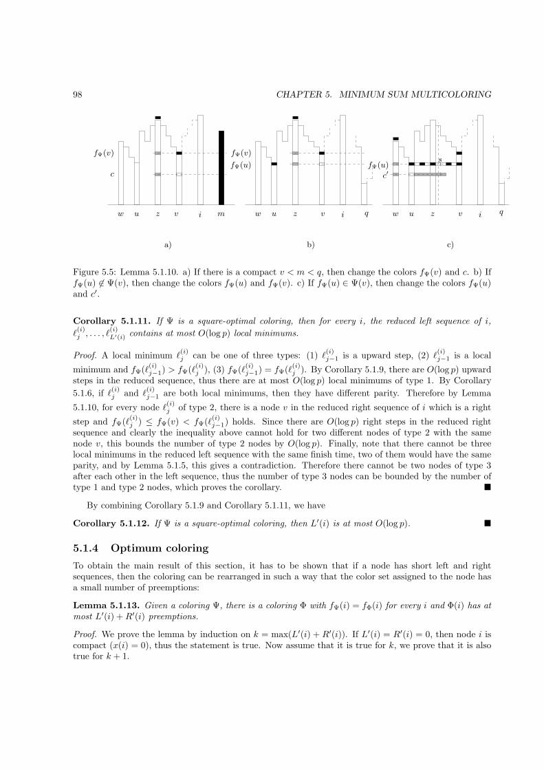
98 CHAPTER 5. MINIMUM SUM MULTICOLORING
m z zz v vv i ii u uu w ww q q
c c′fΨ(u) fΨ(u)
fΨ(v)fΨ(v)s
a) c)b)
Figure 5.5: Lemma 5.1.10. a) If there is a compact v < m < q, then change the colors fΨ(v) and c. b) IffΨ(u) 6∈ Ψ(v), then change the colors fΨ(u) and fΨ(v). c) If fΨ(u) ∈ Ψ(v), then change the colors fΨ(u)and c′.
Corollary 5.1.11. If Ψ is a square-optimal coloring, then for every i, the reduced left sequence of i,
ℓ(i)j , . . . , ℓ
(i)L′(i) contains at most O(log p) local minimums.
Proof. A local minimum ℓ(i)j can be one of three types: (1) ℓ
(i)j−1 is a upward step, (2) ℓ
(i)j−1 is a local
minimum and fΨ(ℓ(i)j−1) > fΨ(ℓ
(i)j ), (3) fΨ(ℓ
(i)j−1) = fΨ(ℓ
(i)j ). By Corollary 5.1.9, there are O(log p) upward
steps in the reduced sequence, thus there are at most O(log p) local minimums of type 1. By Corollary
5.1.6, if ℓ(i)j and ℓ
(i)j−1 are both local minimums, then they have different parity. Therefore by Lemma
5.1.10, for every node ℓ(i)j of type 2, there is a node v in the reduced right sequence of i which is a right
step and fΨ(ℓ(i)j ) ≤ fΨ(v) < fΨ(ℓ
(i)j−1) holds. Since there are O(log p) right steps in the reduced right
sequence and clearly the inequality above cannot hold for two different nodes of type 2 with the samenode v, this bounds the number of type 2 nodes by O(log p). Finally, note that there cannot be threelocal minimums in the reduced left sequence with the same finish time, two of them would have the sameparity, and by Lemma 5.1.5, this gives a contradiction. Therefore there cannot be two nodes of type 3after each other in the left sequence, thus the number of type 3 nodes can be bounded by the number oftype 1 and type 2 nodes, which proves the corollary. �
By combining Corollary 5.1.9 and Corollary 5.1.11, we have
Corollary 5.1.12. If Ψ is a square-optimal coloring, then L′(i) is at most O(log p). �
5.1.4 Optimum coloring
To obtain the main result of this section, it has to be shown that if a node has short left and rightsequences, then the coloring can be rearranged in such a way that the color set assigned to the node hasa small number of preemptions:
Lemma 5.1.13. Given a coloring Ψ, there is a coloring Φ with fΨ(i) = fΦ(i) for every i and Φ(i) has atmost L′(i) +R′(i) preemptions.
Proof. We prove the lemma by induction on k = max(L′(i) + R′(i)). If L′(i) = R′(i) = 0, then node i iscompact (x(i) = 0), thus the statement is true. Now assume that it is true for k, we prove that it is alsotrue for k + 1.
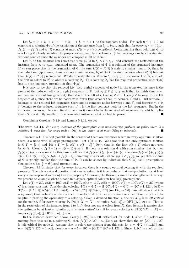
5.1. NUMBER OF PREEMPTIONS 99
Let b0 = 0 < b1 < b2 < · · · < bl−1 < bl = n + 1 be the compact nodes. For each 0 ≤ j < l, weconstruct a coloring Φj of the restriction of the instance from bj to bj+1, such that for every bj ≤ i ≤ bj+1,fΦj
(i) = fΨ(i) and Φj(i) contains at most L′(i) +R′(i) preemptions. Concatenating these colorings Φj toa coloring Φ clearly satisfies the properties required by the lemma. (The colorings can be concatenatedwithout conflict since the bj nodes are compact in all of them.)
Let m be the smallest non-zero finish time fΨ(i) in bj ≤ i ≤ bj+1 and consider the restriction of theinstance from bj to bj+1, truncated at m. The truncation of Ψ is a solution of the truncated instance.If we can prove that in the truncation of Ψ, the sum L′(i) + R′(i) is strictly smaller than in Ψ, then, bythe induction hypotheses, there is an optimum coloring Φ′
j of the truncated instance where Φ′j(i) has less
than L′(i) + R′(i) preemptions. We do a parity shift of Ψ from bj to bj+1 in the range 1 to m, and addthe first m colors to Φ′
j to obtain a coloring Φj. This coloring Φj has the required properties, since Φj(i)has at most one more preemption than Φ′
j(i).It is easy to see that the reduced left (resp. right) sequence of node i in the truncated instance is the
prefix of the reduced left (resp. right) sequence in Ψ. Let bj ≤ i′ ≤ bj+1 such that its finish time is m,and assume without loss generality that it is to the left of i, that is, i′ < i. Clearly i′ belongs to the leftsequence of i, since there are no nodes with finish time smaller than m between i′ and i. Furthermore, i′
belongs to the reduced left sequence: there are no compact nodes between i and i′, and because m > 0,i′ belongs to the reduced sequence even if it is the first compact node in the left sequence. But in thetruncated instance, i′ has zero finish time, thus it cannot be in the reduced left sequence of i, which impliesthat L′(i) is strictly smaller in the truncated instance, what we had to prove. �
Combining Corollary 5.1.9 and Lemma 5.1.13, we get
Theorem 5.1.14. For every instance of the preemptive sum multicoloring problem on paths, there is asolution Ψ such that for every node i, Ψ(i) is the union of at most O(log p) intervals. �
Theorem 5.1.14 is best possible in the sense that there are instances where in every optimum solutionthere is a node with Θ(log p) preemptions. Let x(i) = 4i. We show that the only optimum solutionis Ψ(1) = [1, 4] and Ψ(i + 1) = [1, x(i) + x(i + 1)] \ Ψ(i), that is, the first x(i + 1) colors not usedby Ψ(i). Clearly, fΨ(i + 1) = x(i + 1) + x(i). If there is a solution Φ with sum smaller that Ψ, thenfΦ(i) < fΨ(i) for some i. In this case it follows that fΦ(i−1) ≥ x(i−1)+x(i), therefore fΦ(i−1)+fΦ(i) ≥x(i− 1) +x(i) +x(i) > fΨ(i) + fΨ(i− 1). Summing this for all i where fΦ(i) < fΨ(i), we get that the sumof Ψ is strictly smaller than the sum of Φ. It can be shown by induction that Ψ(2i) has i preemptions,thus node n has n
2 = Θ(log p) preemptions.Theorem 5.1.14 states that for every instance, there is a square-optimal coloring Ψ with the required
property. There is a natural question that can be asked: is it true perhaps that every solution (or at leastevery square-optimal solution) has this property? However, the theorem cannot be strengthened this way:we present an example where a node in a square-optimal solution has Θ(p) preemptions.
Let x(1) = 2C, x(2) = 10C, x(3) = 100C, x(4) = 11C, x(5) = 100C, x(6) = 10C, x(7) = 2C, whereC is a large constant. Consider the coloring Ψ(1) = Ψ(7) = [1, 2C],Ψ(2) = Ψ(6) = [2C + 1, 12C],Ψ(3) =Ψ(5) = [1, C]∪ [12C+ 1, 111C],Ψ(4) = [C+ 1, 2C]∪ [2C+ 1, 12C] (see Figure 5.6). We will show that Ψ isa square-optimal solution of the instance. In order to do this, we introduce a new definition, which will behelpful in proving the optimality of a coloring. Given a demand function x, the set X ⊆ N is left criticalfor the node i, if for every coloring Ψ, |Ψ(i)∩X | = |X |−α implies fΨ([1, i]) ≥ OPT([1, i], x) +α. That is,in the restriction of the instance from 1 to i, if i does not use α colors from X , then its sum is greater thatthe optimum by at least α. Similarly, X is right critical for i, if for every coloring Ψ, |Ψ(i)∩X | = |X | −αimplies fΨ([i, n]) ≥ OPT([i, n], x) + α.
In the instance described above, clearly [1, 2C] is a left critical set for node 1, since if α colors aremissing from this set in a coloring Φ, then fΦ(1) ≥ 2C + α. Next we show that the set [2C + 1, 12C]is left critical for node 2. Assume that α colors are missing from this set: let a = |Φ(2) ∩ [1, 2C]| andb = |Φ(2) ∩ [12C + 1,∞]|, clearly α = a+ b = 10C − |Φ(2) ∩ [2C + 1, 12C]|. Since [1, 2C] is a left critical
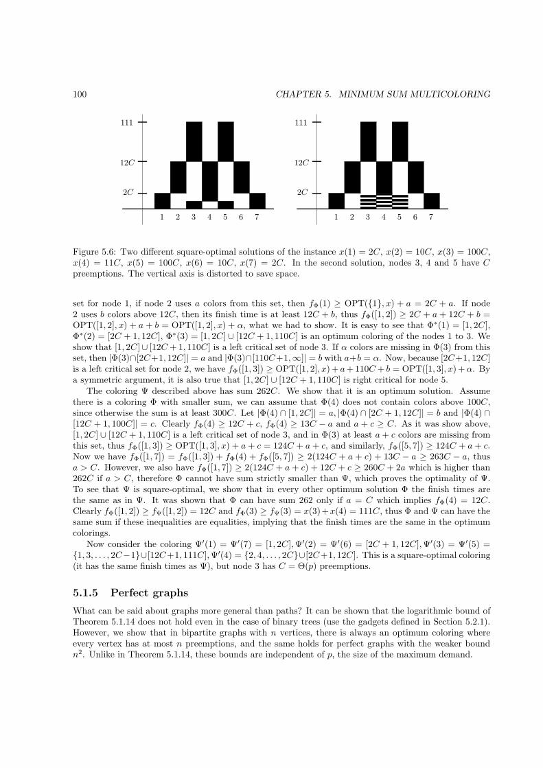
100 CHAPTER 5. MINIMUM SUM MULTICOLORING
11
2C 2C
12C12C
111 111
3 37 76 65 54 42 2
Figure 5.6: Two different square-optimal solutions of the instance x(1) = 2C, x(2) = 10C, x(3) = 100C,x(4) = 11C, x(5) = 100C, x(6) = 10C, x(7) = 2C. In the second solution, nodes 3, 4 and 5 have Cpreemptions. The vertical axis is distorted to save space.
set for node 1, if node 2 uses a colors from this set, then fΦ(1) ≥ OPT({1}, x) + a = 2C + a. If node2 uses b colors above 12C, then its finish time is at least 12C + b, thus fΦ([1, 2]) ≥ 2C + a+ 12C + b =OPT([1, 2], x) + a + b = OPT([1, 2], x) + α, what we had to show. It is easy to see that Φ∗(1) = [1, 2C],Φ∗(2) = [2C + 1, 12C], Φ∗(3) = [1, 2C] ∪ [12C + 1, 110C] is an optimum coloring of the nodes 1 to 3. Weshow that [1, 2C]∪ [12C + 1, 110C] is a left critical set of node 3. If α colors are missing in Φ(3) from thisset, then |Φ(3)∩[2C+1, 12C]| = a and |Φ(3)∩[110C+1,∞]| = b with a+b = α. Now, because [2C+1, 12C]is a left critical set for node 2, we have fΦ([1, 3]) ≥ OPT([1, 2], x) + a+ 110C+ b = OPT([1, 3], x) +α. Bya symmetric argument, it is also true that [1, 2C] ∪ [12C + 1, 110C] is right critical for node 5.
The coloring Ψ described above has sum 262C. We show that it is an optimum solution. Assumethere is a coloring Φ with smaller sum, we can assume that Φ(4) does not contain colors above 100C,since otherwise the sum is at least 300C. Let |Φ(4) ∩ [1, 2C]| = a, |Φ(4) ∩ [2C + 1, 12C]| = b and |Φ(4) ∩[12C + 1, 100C]| = c. Clearly fΦ(4) ≥ 12C + c, fΦ(4) ≥ 13C − a and a + c ≥ C. As it was show above,[1, 2C] ∪ [12C + 1, 110C] is a left critical set of node 3, and in Φ(3) at least a+ c colors are missing fromthis set, thus fΦ([1, 3]) ≥ OPT([1, 3], x) + a+ c = 124C + a+ c, and similarly, fΦ([5, 7]) ≥ 124C + a+ c.Now we have fΦ([1, 7]) = fΦ([1, 3]) + fΦ(4) + fΦ([5, 7]) ≥ 2(124C + a + c) + 13C − a ≥ 263C − a, thusa > C. However, we also have fΦ([1, 7]) ≥ 2(124C + a+ c) + 12C + c ≥ 260C + 2a which is higher than262C if a > C, therefore Φ cannot have sum strictly smaller than Ψ, which proves the optimality of Ψ.To see that Ψ is square-optimal, we show that in every other optimum solution Φ the finish times arethe same as in Ψ. It was shown that Φ can have sum 262 only if a = C which implies fΦ(4) = 12C.Clearly fΦ([1, 2]) ≥ fΨ([1, 2]) = 12C and fΦ(3) ≥ fΨ(3) = x(3)+x(4) = 111C, thus Φ and Ψ can have thesame sum if these inequalities are equalities, implying that the finish times are the same in the optimumcolorings.
Now consider the coloring Ψ′(1) = Ψ′(7) = [1, 2C],Ψ′(2) = Ψ′(6) = [2C + 1, 12C],Ψ′(3) = Ψ′(5) ={1, 3, . . . , 2C−1}∪[12C+1, 111C],Ψ′(4) = {2, 4, . . . , 2C}∪[2C+1, 12C]. This is a square-optimal coloring(it has the same finish times as Ψ), but node 3 has C = Θ(p) preemptions.
5.1.5 Perfect graphs
What can be said about graphs more general than paths? It can be shown that the logarithmic bound ofTheorem 5.1.14 does not hold even in the case of binary trees (use the gadgets defined in Section 5.2.1).However, we show that in bipartite graphs with n vertices, there is always an optimum coloring whereevery vertex has at most n preemptions, and the same holds for perfect graphs with the weaker boundn2. Unlike in Theorem 5.1.14, these bounds are independent of p, the size of the maximum demand.
5.1. NUMBER OF PREEMPTIONS 101
First we introduce a well-studied coloring problem, where the number of different colors used has tobe minimized instead of the total sum. In Lemma 5.1.17, we will show why this problem is relevant tothe study of preemptions in minimum sum coloring.
Minimum Makespan Multicoloring
Input: A graph G(V,E) and a color requirement (or length, demand) function x: V → N.
Output: A multicoloring Ψ : V → 2N such that
• Ψ(u) ∩ Ψ(v) = ∅ if u and v are neighbors in G, and
• |Ψ(v)| = x(v).
Goal: The finish time of vertex v in coloring Ψ is the highest color assigned to it, fΨ(v) =max{i : i ∈ Ψ(v)}. The goal is to minimize maxv∈V fΨ(v), the makespan of the coloring Ψ.
In the case of bipartite graphs, an easy argument shows that there is always a minimum makespancoloring without preemptions.
Lemma 5.1.15. If G is bipartite, then for every demand function x, there is a minimum makespancoloring Ψ where every vertex is colored non-preemptively.
Proof. Let S = maxuv∈E(x(u) + x(v)) be the maximum demand appearing on the endpoints of an edge,clearly at least S colors are required for a proper coloring. We show that there is a non-preemptive coloringusing S colors. Let V1 and V2 be the two bipartition classes of the graph. Let Ψ(v) = [1, x(v)] if x ∈ V1
and let Ψ(v) = [S − x(v) + 1, S(v)] if x ∈ V2. This is a proper coloring: if e = uv, then Ψ(u) ∩ Ψ(v) = ∅follows from x(u) + x(v) ≤ S. �
In order to bound the number of preemptions required in perfect graphs, the polyhedral propertiesof perfect graphs will be used. We only sketch the main idea, the reader is referred to [GLS88] for thebackground.
Lemma 5.1.16. If G is a perfect graph with n vertices, then there is a minimum makespan coloring Ψwhere every vertex has at most n− 1 preemptions.
Proof. Denote by S(G) the set of all independent sets in G. Let A be a |S(G)| times n matrix whose rowsare the characteristic vectors of the sets in S(G). Let the components of the n dimensional vector c bethe values of x(v), and consider the following linear program:
max c′x
Ax ≤ 1 (5.1)
x ≥ 0
It can be easily verified that the integer solutions of the dual program corresponds to the solutions of themakespan problem: we select some independent sets, with possibly selecting a set multiple times, suchthat every vertex v is in at least x(v) selected independent sets. If G is a perfect graph, then it is wellknown that this (5.1) is a Totally Dual Integral system. For every integer vector c, the dual program hasan optimum integral basic solution y. Since A has n columns, the basic solution y has at most n nonzerocomponents, thus there are n independent sets S1, . . . , Sn, and n nonnegative integers y1, . . . , yn such thattaking every independent set Si with multiplicity yi covers every vertex v at least x(v) times, and
∑ni=1 yi
is as small as possible. Now we construct a minimum makespan coloring where every vertex has at mostn− 1 preemptions. The first y1 colors are used only on the vertices in S1, the colors from y1 + 1 to y1 + y2are used only in S2 and so on. Obviously, this is a proper coloring using
∑ni=1 yi colors. �
102 CHAPTER 5. MINIMUM SUM MULTICOLORING
If no vertex has finish time between a and b, then we can reorder the colors between a and b with-out increasing the finish time of any of the vertices. In the following lemma, we perform several suchreorderings, to obtain a minimum sum coloring with few preemptions.
Lemma 5.1.17. Assume that G is a graph such that for every demand function x(v), G has a minimummakespan coloring with at most m preemptions at every vertex. Then for every demand function x(v),there is a minimum sum coloring with at most (m+ 1)n preemptions at every vertex.
Proof. Let Ψ be a minimum sum coloring of G, we transform it into a coloring with (m+1)n preemptionsat every vertex, without increasing the sum. More precisely, if the vertices are ordered such that fΨ(v1) ≤fΨ(v2) ≤ · · · ≤ fΨ(vn), then we construct an optimum coloring where every vertex has at most m + 1preemptions between fΨ(vi) and fΨ(vi+1).
Let fi = fΨ(vi) and let f0 = 0. For every 1 ≤ i ≤ n, we perform the following transformation. Letx′i(v) = |Ψ(v)∩ [fi−1 + 1, fi]|, and let Ψ′
i be a minimum makespan coloring of G with demand function x′i.Obviously, Ψ′
i uses most fi − fi−1 colors, and it can be assumed that every vertex in Ψ′i has at most m
preemptions. Now we replace the range of colors [fi−1 + 1, fi] in Ψ with those appearing in Ψ′i. Formally,
if c ∈ [fi−1 + 1, fi], then let c ∈ Ψ∗(v) if and only if c− fi−1 ∈ Ψ′i(v). It is obvious that in Ψ∗(v), there are
at most m+1 preemptions in the range [fi−1 +1, fi] (it is m+1, not only m, since fi can be a preemptionin Ψ∗(v) even if fi− fi−1, the last color of Ψ′(v) is not a preemption). Repeating this procedure for every1 ≤ i ≤ m results in a coloring with at most (m+ 1)n preemptions at every vertex. �
Combining Lemma 5.1.17 with Lemma 5.1.15 and 5.1.16 gives:
Corollary 5.1.18. If G is a perfect graph with n vertices, then there is an optimum minimum sumcoloring where there are at most n2 preemptions at every vertex. Moreover, if G is bipartite, then thesame holds with at most n preemptions. �
Lemma 5.1.16 shows that in the case of perfect graphs, there is always an optimum solution that canbe represented in size polynomial in the length of the input, even if p is not polynomial in the numberof vertices: it is enough to give at most n2 intervals for each of the n vertices. This can serve as apolynomial-size certificate proving that OPT(G) ≤ k, thus
Corollary 5.1.19. The preemptive sum multicoloring for perfect graphs is in NP, even if p is not poly-nomial in n. �
5.2 Complexity of minimum sum multicoloring for trees
In this section we show that minimum sum multicoloring is NP-hard for binary trees. The proof is inspiredby the proof of Theorem 2.2.1 where it is shown that list multicoloring is NP-hard for trees. We will givea similar reduction from the maximum independent set problem. However, when we were reducing tothe list multicoloring problem, we could use the lists to exclude certain colors from the solution. In theminimum sum multicoloring problem there are no such lists, every color can be used at every vertex.Therefore we will construct “penalty gadgets” that can exclude colors by ensuring that if a forbiddencolor is used, then the gadget can be colored only with large penalty. We will also use the color copyingtrick used in Theorem 2.2.2 to make the reduction work for binary trees.
Let us introduce some notations. If V ′ ⊆ V and Ψ is a coloring then let fΨ(V ′) =∑
v∈V ′ fΨ(v).Similarly, x(V ′) =
∑v∈V ′ x(v). The sum of the optimum coloring of (G, x) is denoted by OPT(G, x),
or by OPT(G) if the function x(v) is clear from the context. The notation [a, b] stands for the set{a, a+ 1, . . . , b} if a ≤ b, otherwise it is the empty set.
5.2. COMPLEXITY OF MINIMUM SUM MULTICOLORING FOR TREES 103
5.2.1 The penalty gadgets
The goal of the penalty gadgets is that by connecting such a gadget to a node v, we can force v not to usecertain colors: if node v uses a forbidden color, then the gadget can be colored only with a “very large”penalty.
For offset t, demand size d and penalty C we define a tree Tt,d,C . The root r of this tree will beconnected to some node v. When the root r of this tree uses the set [t + 1, t + d], then the tree canbe colored optimally. On the other hand, if v uses even one color from [t + 1, t + d], then r cannothave the set [t + 1, t + d] and this constrains the gadget in such a way that it can be colored only withfΨ(Tt,d,C) ≥ OPT (Tt,d,C, x) + C. When C is sufficiently large, then this will force v to use colors not in[t+ 1, t+ d].
Proposition 5.2.1. For integers d, C > t ≥ 0 there is a binary tree Tt,d,C and a demand function x(v)such that
1. The root r has demand x(r) = d.
2. Ψ(r) = [t+ 1, t+ d] in every optimum coloring Ψ.
3. If Ψ(r) 6= [t+ 1, t+ d] for a coloring Ψ, then fΨ(Tt,d,C) ≥ OPT(Tt,d,C , x) + C.
4. The demand x of every vertex is polynomially bounded by d and C.
Furthermore, there is an algorithm which, given t, d and C, outputs the tree Tt,d,C, the demand functionx and the value OPT(Tt,d,C, x) in time polynomial in d and C.
Proof. Let k = ⌈log2(C + t)⌉ and C = 2k. Obviously, C + t ≤ C < 2(C + t). The tree Tt,d,C consists of acomplete binary tree and some attached paths. The complete binary tree T0 has k+ 1 levels, the root r ison level 1 and the leaves, ℓ1, ℓ2, . . . , ℓC , are on level k+ 1. Attach a path of k+ 3 nodes to every leaf: node
ℓi (1 ≤ i ≤ C) is connected to path Pi: ai,k+2, ai,k+1, . . . , ai,2, ai,1, ai,0 (nodes ℓi and ai,k+2 are neighbors).
Figure 5.7 shows the construction for t = 2, d = 4, C = 6. Clearly, Tt,d,C has 2C − 1 + (k + 3)C nodes,which is polynomially bounded in C.
We say that a node is of type j if it is either on the jth level of T0 or it is an ai,j for some 1 ≤ i ≤ C.The demand x(v) will depend only on the type of node v. Let
g(0) = t,
g(1) = d,
g(n) = (3d+ t+ C) · 4n−2 for n ≥ 2.
Obviously, g(n) is monotone and it is easy to see that
g(i+ 1) ≥ 3g(i) + t+ C ≥ g(i− 1) + t+ C
for all i ≥ 1 (these inequalities will be used later).For a node v of type i let x(v) = g(i). This implies that x(r) = g(1) = d for the root r. The maximum
value of x(v) is g(k + 2) = (3d+ t+ C) · 4k, which is bounded by a polynomial of d and C.We describe a proper multicoloring Ψ, which will turn out to be the unique optimum solution. The
same color set is assigned to the nodes of the same type. Start with Ψ(v) = [1, t] for every node v of type0. Then color the different types in increasing order: assign to the nodes of type i the first g(i) colors notused by the type i − 1 nodes. This gives a proper coloring since the already colored neighbors of type inodes are type i− 1 nodes. Notice that the root r receives the set [t+ 1, t+ d], as required. It is easy toprove that the finish time of a node v of type i is fΨ(v) = g(i) + g(i− 1) = x(i) + x(i− 1) since there willbe exactly g(i− 1) “skipped” colors and the finish time of nodes of type i is greater then the finish time
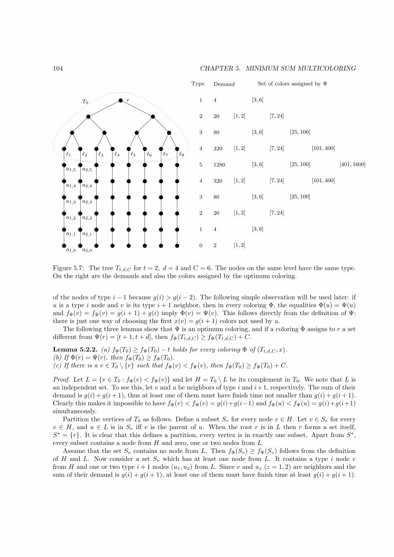
104 CHAPTER 5. MINIMUM SUM MULTICOLORING
ℓ1 ℓ2 ℓ3 ℓ4 ℓ5 ℓ6 ℓ7 ℓ8
a1,5
a1,0
a1,1
a1,2
a1,3
a1,4
a2,5
a2,4
a2,3
a2,2
a2,1
a2,0
rT0
[7, 24]
[7, 24]
[7, 24]
[7, 24]
[25, 100]
[25, 100]
[25, 100]
[101, 400]
[101, 400]
Set of colors assigned by ΨDemand
1280
320
320
80
80
20
20
1
1
5
4
4
4
4
3
3
2
2
20
Type
[1, 2]
[1, 2]
[1, 2]
[1, 2]
[1, 2]
[3, 6]
[3, 6]
[3, 6]
[3, 6]
[3, 6]
[401, 1600]
Figure 5.7: The tree Tt,d,C for t = 2, d = 4 and C = 6. The nodes on the same level have the same type.On the right are the demands and also the colors assigned by the optimum coloring.
of the nodes of type i− 1 because g(i) > g(i− 2). The following simple observation will be used later: ifu is a type i node and v is its type i + 1 neighbor, then in every coloring Φ, the equalities Φ(u) = Ψ(u)and fΦ(v) = fΨ(v) = g(i + 1) + g(i) imply Φ(v) = Ψ(v). This follows directly from the definition of Ψ:there is just one way of choosing the first x(v) = g(i+ 1) colors not used by u.
The following three lemmas show that Ψ is an optimum coloring, and if a coloring Φ assigns to r a setdifferent from Ψ(r) = [t+ 1, t+ d], then fΦ(Tt,d,C) ≥ fΨ(Tt,d,C) + C.
Lemma 5.2.2. (a) fΦ(T0) ≥ fΨ(T0) − t holds for every coloring Φ of (Tt,d,C , x).(b) If Φ(r) = Ψ(r), then fΦ(T0) ≥ fΨ(T0).(c) If there is a v ∈ T0 \ {r} such that fΦ(v) < fΨ(v), then fΦ(T0) ≥ fΨ(T0) + C.
Proof. Let L = {v ∈ T0 : fΦ(v) < fΨ(v)} and let H = T0 \ L be its complement in T0. We note that L isan independent set. To see this, let v and u be neighbors of type i and i+1, respectively. The sum of theirdemand is g(i) + g(i+ 1), thus at least one of them must have finish time not smaller than g(i) + g(i+ 1).Clearly this makes it impossible to have fΦ(v) < fΨ(v) = g(i)+g(i−1) and fΦ(u) < fΨ(u) = g(i)+g(i+1)simultaneously.
Partition the vertices of T0 as follows. Define a subset Sv for every node v ∈ H . Let v ∈ Sv for everyv ∈ H , and u ∈ L is in Sv iff v is the parent of u. When the root r is in L then r forms a set itself,S∗ = {r}. It is clear that this defines a partition, every vertex is in exactly one subset. Apart from S∗,every subset contains a node from H and zero, one or two nodes from L.
Assume that the set Sv contains no node from L. Then fΦ(Sv) ≥ fΨ(Sv) follows from the definitionof H and L. Now consider a set Sv which has at least one node from L. It contains a type i node vfrom H and one or two type i+ 1 nodes (u1, u2) from L. Since v and uz (z = 1, 2) are neighbors and thesum of their demand is g(i) + g(i+ 1), at least one of them must have finish time at least g(i) + g(i+ 1).
5.2. COMPLEXITY OF MINIMUM SUM MULTICOLORING FOR TREES 105
Since uz is in L, we have fΦ(uz) < fΨ(uz) = g(i) + g(i + 1), thus fΦ(v) ≥ g(i) + g(i + 1). Therefore,fΦ(v) − fΨ(v) ≥ (g(i) + g(i+ 1)) − (g(i− 1) + g(i)) = g(i+ 1) − g(i− 1). Since fΨ(uz) = g(i+ 1) + g(i)and x(uz) = g(i+ 1), clearly fΦ(uz) − fΨ(uz) ≥ −g(i). Now
fΦ(Sv) − fΨ(Sv) ≥ (g(i+ 1) − g(i− 1)) − 2g(i) ≥ g(i+ 1) − 3g(i) ≥ C + t,
where the last inequality follows from g(i+ 1) ≥ 3g(i) + C + t.If r is in S∗, then fΦ(S∗) = fΨ(S∗) + (fΦ(r) − fΨ(r)) holds. Therefore fΦ(T0) ≥ fΨ(T0) + (fΦ(r) −
fΨ(r)) ≥ fΨ(T0)− t, since fΦ(r) ≥ d. This proves statement (a), and (b) also follows because Φ(r) = Ψ(r)implies fΦ(r) − fΨ(r) = 0. Furthermore, if fΦ(u) < fΨ(u) for some u ∈ T0 \ {r}, then fΦ(Sv) ≥fΨ(Sv) + C + t for the set Sv of the partition that contains u. This proves statement (c).
�
Lemma 5.2.3. fΦ(Pi) > fΨ(Pi) holds for every coloring Φ 6= Ψ of Tt,d,C and for every 1 ≤ i ≤ C.
Proof. Assume that fΦ(Pi) ≤ fΨ(Pi), define L = {v ∈ Pi : fΦ(v) < fΨ(v)} and H = Pi \ L. IffΦ(Pi) ≤ fΨ(Pi) and Φ is different from Ψ, then there is a v ∈ Pi such that fΦ(v) < fΨ(v), thus L is notempty. As in Lemma 5.2.2, it is easy to see that L is an independent set. The nodes of Pi are partitionedinto |H | classes: if v ∈ H then v is in Sv, if u ∈ L then u is in Sv, where v is the child of u. Notice thatai,0 ∈ H since fΨ(ai,0) = x(ai,0) = g(0) ≤ fΦ(ai,0).
We prove that fΦ(Sv) ≥ fΨ(Sv) for every Sv. If Sv = {v}, then it is clear that fΦ(Sv) ≥ fΨ(Sv) holds.Assume that Sv = {u, v}, node u ∈ L is type j + 1, and v ∈ H (its child) is type j ≥ 0. The finish timeof node v is at least x(u) + x(v) = g(j + 1) + g(j), therefore
fΦ(Sv) ≥ x(u) + (x(u) + x(v)) = g(j + 1) + (g(j + 1) + g(j))
holds. On the other hand, if j ≥ 1, then fΨ(Sv) = (g(j+1)+g(j))+(g(j)+g(j−1)), thus fΦ(Sv) > fΨ(Sv)follows from g(j + 1) > g(j) + g(j − 1). In the case j = 0, we have fΨ(Sv) = t+ (t+ d) = g(j) + (g(j) +g(j + 1)) < fΦ(Sv), since fΦ(Sv) ≥ g(j + 1) + (g(j) + g(j + 1)) = d + (t + d) (recall that t < d). SinceH is not empty, there is at least one subset Sv in the partition with fΦ(Sv) > fΨ(Sv), contradictingfΦ(Pi) ≤ fΨ(Pi). �
Lemma 5.2.4. If Φ(r) 6= Ψ(r) = [t+ 1, t+ d], then fΦ(Tt,d,C) ≥ fΨ(Tt,d,C) + C.
Proof. Denote by P ∗ =⋃Ci=1 Pi = Tt,d,C \ T0 the union of the paths. If there is a node v ∈ T0 \ {r} with
fΦ(v) < fΨ(v), then by part (c) of Lemma 5.2.2 fΦ(T0) ≥ fΨ(T0) + C, and by Lemma 5.2.3 fΦ(P ∗) ≥fΨ(P ∗) follows, which implies fΦ(Tt,d,C) ≥ fΨ(Tt,d,C) +C, and we are done. Therefore it can be assumedthat fΦ(v) ≥ fΨ(v) for every node v ∈ T0\{r}. Furthermore, if there is a v ∈ T0 with fΦ(v) ≥ fΨ(v)+C+t,then fΦ(T0) ≥ fΨ(T0) + C, thus fΦ(P ∗) ≥ fΨ(P ∗) implies fΦ(Tt,d,C) ≥ fΨ(Tt,d,C) + C. In the following,it will be assumed that fΨ(v) ≤ fΦ(v) ≤ fΨ(v) + C + t holds for every v ∈ T0 \ {r}.
Call a vertex v changed in Φ if Φ(v) 6= Ψ(v). The goal is to show that if the root r is changed, then allthe nodes a1,k+2, a2,k+2, . . . , aC,k+2 are changed. Let v be a node of type i in T0 and let u be one of its
children, a node of type i+1. If v is changed, then there is a color j ∈ Φ(v) and j 6∈ Ψ(v). We consider twocases. If j ≤ fΨ(u), then by the fact that j 6∈ Ψ(v) and the way Ψ was defined j ∈ Ψ(u) follows. Thereforeu is also changed since j ∈ Φ(v) implies j 6∈ Φ(u). In the second case, where j > fΨ(u) = g(i+ 1) + g(i)we have
fΦ(v) ≥ j > g(i+ 1) + g(i) = (g(i + 1) − g(i− 1)) + (g(i) + g(i− 1))
= g(i+ 1) − g(i− 1) + fΨ(v) ≥ fΨ(v) + C + t,
contradicting the assumption fΦ(v) ≤ fΨ(v) + C + t.
106 CHAPTER 5. MINIMUM SUM MULTICOLORING
Assume that fΦ(Tt,d,C) < fΨ(Tt,d,C) + C. By applying the previous result inductively, one finds that
all the leaves ℓi and their children ai,k+2 (1 ≤ i ≤ C) are changed. Lemma 5.2.3 ensures that Φ is not
an optimum coloring of Pi, thus fΦ(Pi) ≥ fΨ(Pi) + 1 and fΦ(P ∗) ≥ fΨ(P ∗) + C ≥ fΨ(P ∗) + C + t. ByLemma 5.2.2, fΦ(T0) ≥ fΨ(T0) − t, hence fΦ(Tt,d,C) ≥ fΨ(Tt,d,C) + C. �
To finish the proof of Prop. 5.2.1, we have to show that requirements 2 and 3 hold. If Φ(r) = Ψ(r),then by part (b) of Lemma 5.2.2 and by Lemma 5.2.3, fΦ(Tt,d,C) ≥ fΨ(Tt,d,C). If Φ(r) 6= Ψ(r), then byLemma 5.2.4, fΦ(Tt,d,C) ≥ fΨ(Tt,d,C) + C. Therefore the coloring Ψ is an optimum coloring and the treesatisfies the requirements of the proposition.
Clearly, the tree Tt,d,C and the demand function x can be constructed in polynomial time. The sumof the optimum solution can be also calculated, by adding the appropriate finish time of every node. �
5.2.2 The reduction
We will reduce the maximum independent set problem to the minimum sum coloring problem in binarytrees. In the decision version of the minimum sum coloring problem, the input is a graph G, a demandfunction x(v), and an integer K. The question is whether there exists a multicoloring Ψ with sum lessthan K. The reduction is based on the proof of Theorem 2.2.2. The penalty gadgets Tt,d,C of Section 5.2.1are used to imitate the effect of the color lists.
More precisely, the penalty gadget is used in two different ways: as a lower penalty gadget and asan upper penalty gadget. The lower penalty gadget TLd,C is a tree T0,d,C. By connecting the root of sucha tree to a node v, the node v is forced to use only colors greater than d: otherwise the gadget can becolored only with a penalty C. A tree is a tree of type TL if it is the tree TLd,C for some d and C.
The upper penalty gadget TUd,C is a tree Td,C,C . If this gadget is connected to a node v, then this forcesv to use only colors not greater than d. If v uses only colors at most d, then its finish time is at most d,and the gadget can be colored optimally. If v uses a color greater than d but not greater than d+C, thenthe gadget can be colored only with penalty C. If v uses colors greater than d+C, then it has finish timeat least d+ C, which is a penalty of at least C compared to the case when v uses only colors at most d.
Theorem 5.2.5. The minimum sum preemptive multicoloring problem is NP-complete on binary treeswhen the value of the demand function is polynomially bounded.
Proof. Let a graph G(V,E) and an integer k be given. Denote n = |V |, m = |E|, and let C = 8mn. Letintegers ui,1 < ui,2 denote the two end vertices of the ith edge in G.
We define a binary tree T , which consists of a core T and some attached subtrees of type TL and TU .We start with a path of 2m−1 nodes, a1, b1, a2, b2, . . . , am−1, bm−1, am. Define x(ai) = k (1 ≤ i ≤ m) andx(bi) = C + n− k (1 ≤ i ≤ m− 1). For every 1 ≤ i ≤ m attach a path of 6 nodes to ai. Let these nodesbe ci,1, di,1, ci,2, di,2, ci,3, di,3. Let x(ci,j) = 1, x(di,j) = C + n − 1 (j = 1, 2) and x(ci,3) = 1, x(di,3) =
ui,2 − ui,1 − 1. Clearly, x(v) ≥ 0 for every node v. This completes the definition of T . Now attach trees
of type TL and TU to T as follows (see Figure 5.8):
• a TUC+n,2C to every node bi (1 ≤ i ≤ m− 1),
• a TUn,C to the node a1,
• a TUC+n,2C to every node di,j (1 ≤ i ≤ m, j = 1, 2),
• a TUui,2+1,C to every node ci,1 (1 ≤ i ≤ m),
• a TLui,1−1,C to every node ci,2 (1 ≤ i ≤ m),
• a TLui,1,Cand a TUui,2−1,C to every node di,3 (1 ≤ i ≤ m).
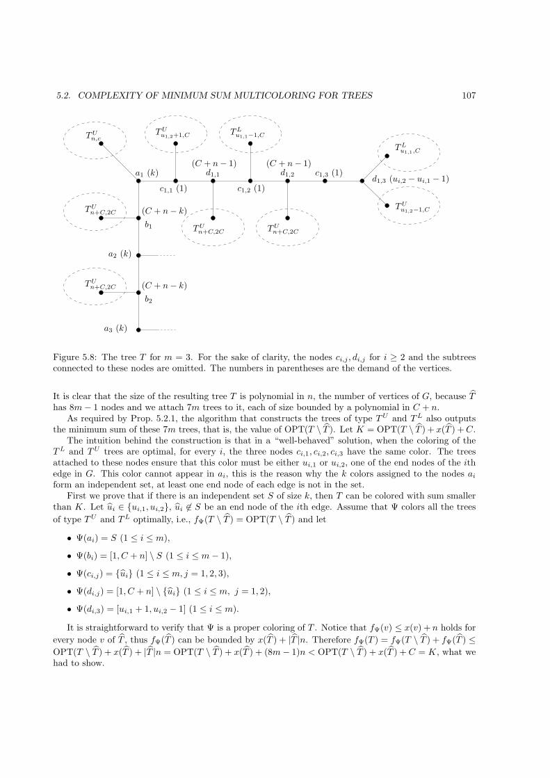
5.2. COMPLEXITY OF MINIMUM SUM MULTICOLORING FOR TREES 107
TUn,c
TUu1,2−1,C
TLu1,1,C
TUn+C,2C
TUn+C,2C
a3 (k)
a2 (k)
b1
b2
(C + n− k)
(C + n− k)
TUn+C,2CTUn+C,2C
c1,3 (1)
c1,1 (1) c1,2 (1)d1,3 (ui,2 − ui,1 − 1)
a1 (k) d1,2
(C + n− 1) (C + n− 1)d1,1
TLu1,1−1,CTUu1,2+1,C
Figure 5.8: The tree T for m = 3. For the sake of clarity, the nodes ci,j , di,j for i ≥ 2 and the subtreesconnected to these nodes are omitted. The numbers in parentheses are the demand of the vertices.
It is clear that the size of the resulting tree T is polynomial in n, the number of vertices of G, because Thas 8m− 1 nodes and we attach 7m trees to it, each of size bounded by a polynomial in C + n.
As required by Prop. 5.2.1, the algorithm that constructs the trees of type TU and TL also outputsthe minimum sum of these 7m trees, that is, the value of OPT(T \ T ). Let K = OPT(T \ T ) + x(T ) +C.
The intuition behind the construction is that in a “well-behaved” solution, when the coloring of theTL and TU trees are optimal, for every i, the three nodes ci,1, ci,2, ci,3 have the same color. The treesattached to these nodes ensure that this color must be either ui,1 or ui,2, one of the end nodes of the ithedge in G. This color cannot appear in ai, this is the reason why the k colors assigned to the nodes aiform an independent set, at least one end node of each edge is not in the set.
First we prove that if there is an independent set S of size k, then T can be colored with sum smallerthan K. Let ui ∈ {ui,1, ui,2}, ui 6∈ S be an end node of the ith edge. Assume that Ψ colors all the trees
of type TU and TL optimally, i.e., fΨ(T \ T ) = OPT(T \ T ) and let
• Ψ(ai) = S (1 ≤ i ≤ m),
• Ψ(bi) = [1, C + n] \ S (1 ≤ i ≤ m− 1),
• Ψ(ci,j) = {ui} (1 ≤ i ≤ m, j = 1, 2, 3),
• Ψ(di,j) = [1, C + n] \ {ui} (1 ≤ i ≤ m, j = 1, 2),
• Ψ(di,3) = [ui,1 + 1, ui,2 − 1] (1 ≤ i ≤ m).
It is straightforward to verify that Ψ is a proper coloring of T . Notice that fΨ(v) ≤ x(v) + n holds for
every node v of T , thus fΨ(T ) can be bounded by x(T ) + |T |n. Therefore fΨ(T ) = fΨ(T \ T ) + fΨ(T ) ≤
OPT(T \ T ) + x(T ) + |T |n = OPT(T \ T ) + x(T ) + (8m− 1)n < OPT(T \ T ) + x(T ) + C = K, what wehad to show.
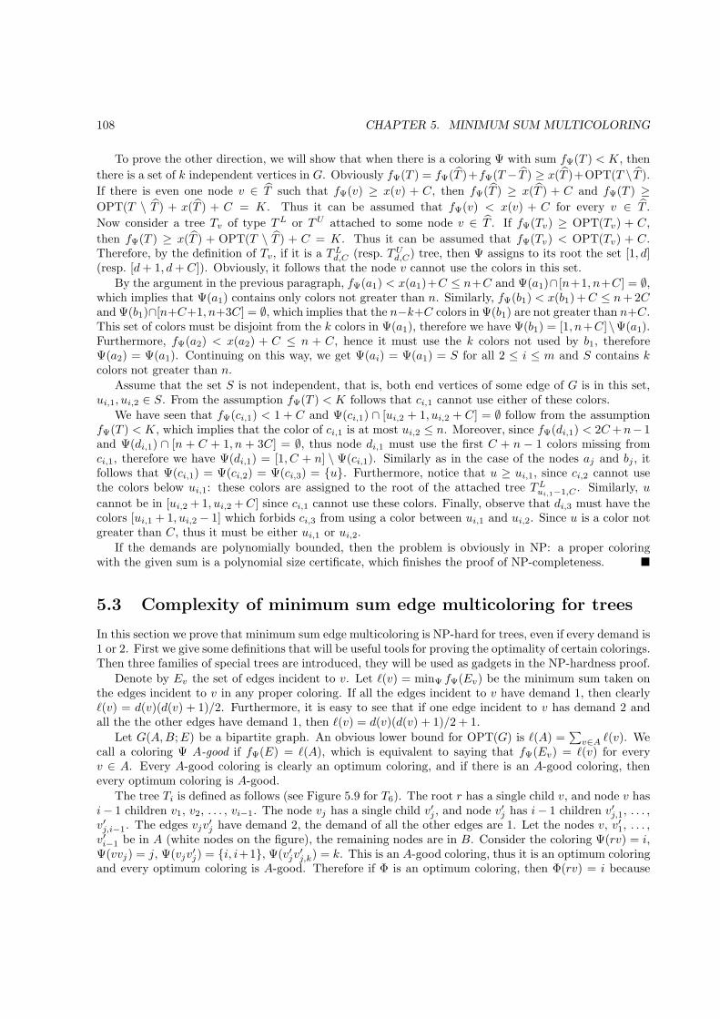
108 CHAPTER 5. MINIMUM SUM MULTICOLORING
To prove the other direction, we will show that when there is a coloring Ψ with sum fΨ(T ) < K, then
there is a set of k independent vertices in G. Obviously fΨ(T ) = fΨ(T )+fΨ(T − T ) ≥ x(T )+OPT(T \ T ).
If there is even one node v ∈ T such that fΨ(v) ≥ x(v) + C, then fΨ(T ) ≥ x(T ) + C and fΨ(T ) ≥
OPT(T \ T ) + x(T ) + C = K. Thus it can be assumed that fΨ(v) < x(v) + C for every v ∈ T .
Now consider a tree Tv of type TL or TU attached to some node v ∈ T . If fΨ(Tv) ≥ OPT(Tv) + C,
then fΨ(T ) ≥ x(T ) + OPT(T \ T ) + C = K. Thus it can be assumed that fΨ(Tv) < OPT(Tv) + C.Therefore, by the definition of Tv, if it is a TLd,C (resp. TUd,C) tree, then Ψ assigns to its root the set [1, d](resp. [d+ 1, d+ C]). Obviously, it follows that the node v cannot use the colors in this set.
By the argument in the previous paragraph, fΨ(a1) < x(a1)+C ≤ n+C and Ψ(a1)∩ [n+1, n+C] = ∅,which implies that Ψ(a1) contains only colors not greater than n. Similarly, fΨ(b1) < x(b1) +C ≤ n+ 2Cand Ψ(b1)∩[n+C+1, n+3C] = ∅, which implies that the n−k+C colors in Ψ(b1) are not greater than n+C.This set of colors must be disjoint from the k colors in Ψ(a1), therefore we have Ψ(b1) = [1, n+C]\Ψ(a1).Furthermore, fΨ(a2) < x(a2) + C ≤ n + C, hence it must use the k colors not used by b1, thereforeΨ(a2) = Ψ(a1). Continuing on this way, we get Ψ(ai) = Ψ(a1) = S for all 2 ≤ i ≤ m and S contains kcolors not greater than n.
Assume that the set S is not independent, that is, both end vertices of some edge of G is in this set,ui,1, ui,2 ∈ S. From the assumption fΨ(T ) < K follows that ci,1 cannot use either of these colors.
We have seen that fΨ(ci,1) < 1 + C and Ψ(ci,1) ∩ [ui,2 + 1, ui,2 + C] = ∅ follow from the assumptionfΨ(T ) < K, which implies that the color of ci,1 is at most ui,2 ≤ n. Moreover, since fΨ(di,1) < 2C+n− 1and Ψ(di,1) ∩ [n + C + 1, n + 3C] = ∅, thus node di,1 must use the first C + n − 1 colors missing fromci,1, therefore we have Ψ(di,1) = [1, C + n] \ Ψ(ci,1). Similarly as in the case of the nodes aj and bj , itfollows that Ψ(ci,1) = Ψ(ci,2) = Ψ(ci,3) = {u}. Furthermore, notice that u ≥ ui,1, since ci,2 cannot usethe colors below ui,1: these colors are assigned to the root of the attached tree TLui,1−1,C . Similarly, u
cannot be in [ui,2 + 1, ui,2 +C] since ci,1 cannot use these colors. Finally, observe that di,3 must have thecolors [ui,1 + 1, ui,2 − 1] which forbids ci,3 from using a color between ui,1 and ui,2. Since u is a color notgreater than C, thus it must be either ui,1 or ui,2.
If the demands are polynomially bounded, then the problem is obviously in NP: a proper coloringwith the given sum is a polynomial size certificate, which finishes the proof of NP-completeness. �
5.3 Complexity of minimum sum edge multicoloring for trees
In this section we prove that minimum sum edge multicoloring is NP-hard for trees, even if every demand is1 or 2. First we give some definitions that will be useful tools for proving the optimality of certain colorings.Then three families of special trees are introduced, they will be used as gadgets in the NP-hardness proof.
Denote by Ev the set of edges incident to v. Let ℓ(v) = minΨ fΨ(Ev) be the minimum sum taken onthe edges incident to v in any proper coloring. If all the edges incident to v have demand 1, then clearlyℓ(v) = d(v)(d(v) + 1)/2. Furthermore, it is easy to see that if one edge incident to v has demand 2 andall the the other edges have demand 1, then ℓ(v) = d(v)(d(v) + 1)/2 + 1.
Let G(A,B;E) be a bipartite graph. An obvious lower bound for OPT(G) is ℓ(A) =∑
v∈A ℓ(v). Wecall a coloring Ψ A-good if fΨ(E) = ℓ(A), which is equivalent to saying that fΨ(Ev) = ℓ(v) for everyv ∈ A. Every A-good coloring is clearly an optimum coloring, and if there is an A-good coloring, thenevery optimum coloring is A-good.
The tree Ti is defined as follows (see Figure 5.9 for T6). The root r has a single child v, and node v hasi− 1 children v1, v2, . . . , vi−1. The node vj has a single child v′j , and node v′j has i− 1 children v′j,1, . . . ,v′j,i−1. The edges vjv
′j have demand 2, the demand of all the other edges are 1. Let the nodes v, v′1, . . . ,
v′i−1 be in A (white nodes on the figure), the remaining nodes are in B. Consider the coloring Ψ(rv) = i,Ψ(vvj) = j, Ψ(vjv
′j) = {i, i+1}, Ψ(v′jv
′j,k) = k. This is an A-good coloring, thus it is an optimum coloring
and every optimum coloring is A-good. Therefore if Φ is an optimum coloring, then Φ(rv) = i because
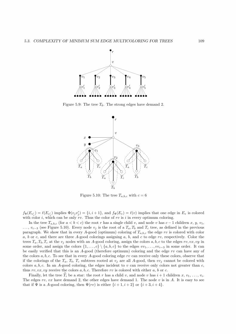
5.3. COMPLEXITY OF MINIMUM SUM EDGE MULTICOLORING FOR TREES 109
v′1 v′2 v′3 v′4 v′5
v5v4v3v2v1
r
v
Figure 5.9: The tree T6. The strong edges have demand 2.
v
Tc
TcTc
Ta
TaTa
Tb
TbTb
v3
v2
v1
x
y
r
Figure 5.10: The tree Ta,b,c with c = 6
fΦ(Ev′j) = ℓ(Ev′
j) implies Φ(vjv
′j) = {i, i+ 1}, and fΦ(Ev) = ℓ(v) implies that one edge in Ev is colored
with color i, which can be only rv. Thus the color of rv is i in every optimum coloring.
In the tree Ta,b,c (for a < b < c) the root r has a single child v, and node v has c− 1 children x, y, v1,. . . , vc−3 (see Figure 5.10). Every node vj is the root of a Ta, Tb and Tc tree, as defined in the previousparagraph. We show that in every A-good (optimum) coloring of Ta,b,c the edge rv is colored with colora, b or c, and there are three A-good colorings assigning a, b, and c to edge rv, respectively. Color thetrees Ta, Tb, Tc at the vj nodes with an A-good coloring, assign the colors a, b, c to the edges rv, vx, vy insome order, and assign the colors {1, . . . , c} \ {a, b, c} to the edges vv1, . . . , vvc−3 in some order. It canbe easily verified that this is an A-good (therefore optimum) coloring and the edge rv can have any ofthe colors a, b, c. To see that in every A-good coloring edge rv can receive only these colors, observe thatif the colorings of the Ta, Tb, Tc subtrees rooted at vj are all A-good, then vvj cannot be colored withcolors a, b, c. In an A-good coloring, the edges incident to v can receive only colors not greater than c,thus rv, vx, vy receive the colors a, b, c. Therefore rv is colored with either a, b or c.
Finally, let the tree Ti be a star: the root r has a child v, and node v has i+ 1 children x, v1, . . . , vi.The edges rv, vx have demand 2, the other edges have demand 1. The node v is in A. It is easy to seethat if Ψ is a A-good coloring, then Ψ(rv) is either {i+ 1, i+ 2} or {i+ 3, i+ 4}.
110 CHAPTER 5. MINIMUM SUM MULTICOLORING
Theorem 5.3.1. The minimum sum edge multicoloring problem is NP-hard for trees, even if every demandis 1 or 2.
Proof. The reduction is from 3-occurrence 3SAT, it can be assumed that every variable occurs at mosttwice positively and at most twice negatively. Given a formula with n variables and m clauses, we constructa tree T and a demand function such that the tree has an A-good coloring (i.e., a coloring with sum atmost ℓ(A)) if and only if the formula is satisfiable.
Consider the variable xk (0 ≤ k < n), which is the hth literal of the ith clause. Let di,h be 4k + 1 ifthis is the first positive occurrence of xk, 4k + 2 if this is the second positive occurrence, 4k + 3 if thisis the first negated occurrence, and 4k + 4 if this is the second negated occurrence. Tree T has a node rwhich is the root of n + m trees. To each variable xj corresponds a tree T4j , and to each clause i a treeTdi,1,di,2,di,3 . This defines T and its demand function.
Assume that a coloring is A-good, then it is an A-good coloring of all the n+m subtrees (since r 6∈ A).
Therefore the root edge of T4j corresponding to variable xj uses either the set {4j + 1, 4j + 2} or the set{4j+ 3, 4j+ 4}. Assign to the variable xj the value “false” in the first case and “true” in the second case.This will be a satisfying assignment: if the root edge of the tree corresponding to clause i uses a color from{4j+ 1, 4j+ 2, 4j+ 3, 4j+ 4}, then variable xj satisfies clause i. More precisely, if it uses 4j+ 1 or 4j+ 2(resp. 4j + 3 or 4j + 4), then xj has the value “true” (resp. ”false”), and because of the construction, xjappears in clause i positively (resp. negatively).
To prove the other direction, given a satisfying assignment, we construct an A-good coloring of thetree. Take an A-good coloring of the subtree T4j corresponding to variable xj such that its root edge usesthe colors {4j + 1, 4j + 2} (resp. {4j + 3, 4j + 4}) if xj is “false” (resp. ”true”). Since every clause issatisfied by some variable, we can choose an A-good coloring for each subtree corresponding to a clausesuch that it does not conflict with any of the trees corresponding to the variables. Clearly, this will be anA-good coloring of the tree.
We have reduced the known NP-complete problem to the minimum sum edge multicoloring problem.The reduction can be done in polynomial time, thus minimum sum edge multicoloring is NP-hard. �
We note that in the proof, the proposed optimum coloring colors non-preemptively every edge withdemand 2. Thus the reduction works even if we impose the additional constraint of non-preemptivecoloring.
Corollary 5.3.2. The non-preemptive version of minimum sum edge multicoloring is NP-hard for trees,even if every demand is 1 or 2. �
5.4 Approximating minimum sum multicoloring on the edges of
trees
In this section we consider the minimum sum edge multicoloring problem restricted to trees. We have seenin Section 5.3 that, unlike the unit demand case, minimum sum edge multicoloring is NP-hard for treesif the demands are allowed to be at most 2. On the other hand, in this section we show that the problemis polynomial time solvable in trees if every demand is the same. This is a consequence of the followingscaling property of minimum sum edge multicoloring in trees: if the demand of every edge is multipliedby the same integer q, then the sum of the optimum solution increases by a factor of q. It is easy to seethat the sum changes by at most a factor of q, the interesting thing is that this factor is exactly q. Themain result in this section is a polynomial time approximation scheme (PTAS) for minimum sum edgemulticoloring in trees.
Recently, the vertex coloring version of minimum sum multicoloring was investigated by several pa-pers [HKP+03, Mar02, HK02, BNHK+00, Kov04], but the edge coloring problem is only mentioned in
5.4. APPROXIMATING MINIMUM SUM MULTICOLORING ON THE EDGES OF TREES 111
[BNHK+00] and [Kub96]. In [HK02, HKP+03] PTAS is given for the vertex coloring version of the prob-lem in the case when the graph is a tree, partial k-tree, or a planar graph. One of their main tools isthe decomposition of colors into layers of geometrically increasing size. This method will be used here aswell. However, most of the other tools in [HK02, HKP+03] cannot be applied in our case, since those toolsassume that the graph can be colored with a constant number of colors. In our case this is not necessarilytrue: if the maximum degree of the tree can be arbitrary, then the line graph of the tree can containarbitrarily large cliques. On one hand, these large cliques make the tools developed for partial k-treesimpossible or very difficult to apply. On the other hand, a large clique helps us in finding an approximatesolution: since the sum of a large clique has to be very large in every coloring (it grows quadratically inthe size of the clique), more errors can be tolerated in an approximate solution, and this gives us moreelbow space in constructing a good approximation.
In Section 5.4.1 we introduce notations and give some preliminary results. The scaling property fortrees is proved in Section 5.4.2. Section 5.4.3 gives a simple PTAS for the problem if the demand of everyedge in the tree is bounded by a constant, while Section 5.4.4 deals with the case where the maximumdegree of the tree is bounded by a constant. Finally, Section 5.4.5 combines the ideas presented in thepreceding two sections to give a PTAS for the general case, where the demands and the degrees can bearbitrary.
In [Mar04f] the results of this section are generalized: the PTAS for trees is extended to partial k-treesand planar graphs. The approximation scheme for partial k-trees is very similar to the one presentedhere for trees, although some new ideas and techniques are also required. Using the layering technique ofBaker [Bak94], the PTAS for partial k-trees can be used to obtain a PTAS for planar graphs. We statehere these results without proof:
Theorem 5.4.1 ([Mar04f]). For every ǫ > 0 and every integer k, there is a linear time (1 + ǫ)-approximation algorithm for solving minimum sum edge multicoloring on partial k-trees.
Theorem 5.4.2 ([Mar04f]). For every ǫ > 0, there is a linear time (1 + ǫ)-approximation algorithm forsolving minimum sum edge multicoloring on planar graphs.
5.4.1 Preliminaries
We extend the notion of finish time to a set E′ of edges by defining fΨ(E′) =∑e∈E′ fΨ(e). Given a graph
G and a demand function x(e) on the edges of G, the minimum sum that can be achieved is denoted byOPT(G, x), or by simply OPT(G), if the demand function is clear from the context.
For a minimization problem, algorithm A is an α-approximation algorithm if it always produces asolution with cost at most α times the optimum. A polynomial time approximation scheme (PTAS) is analgorithm that has a parameter ǫ such that for every ǫ > 0 it produces an (1 + ǫ)-approximate solution,and the running time is polynomial in n for every fixed ǫ, e.g., O(n1/ǫ). A linear time PTAS runs in timeO(f(ǫ)n) where f is an arbitrary function. When designing a PTAS, it can be assumed that ǫ is smallerthan some fixed constant ǫ0. In the following it is assumed that ǫ is sufficiently small and 1/ǫ is an integer.Appendix A.2 contains some more background on approximation algorithms.
Henceforth the graph G is a rooted tree with root r. The root is assumed to be a node of degreeone, the root edge is the edge incident to r. Every edge has an upper node (closer to r) and a lower node(farther from r). Edge f is a child edge of edge e if the upper node of f is the same as the lower node ofe. In this case, edge e is the parent edge of edge f . A node is a leaf node if it has no children, and an edgeis a leaf edge if its lower node is a leaf node. The subtree Te consists of the edge e and the subtree rootedat the lower node of e.
A top-down traversal of the edges is an ordering of the edges in such a way that every edge appearslater than its parent edge. Similarly, in a bottom-up traversal of the edges every edge appears before itsparent. It is clear that such orderings exist and can be found in linear time.
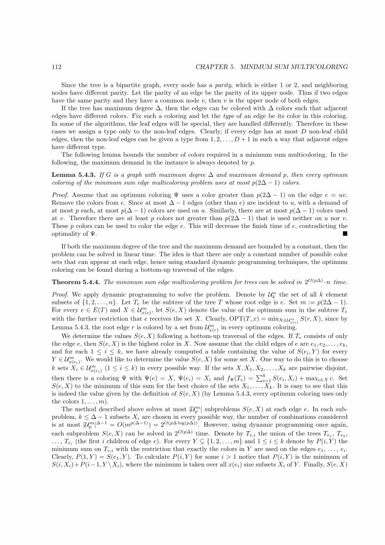
112 CHAPTER 5. MINIMUM SUM MULTICOLORING
Since the tree is a bipartite graph, every node has a parity, which is either 1 or 2, and neighboringnodes have different parity. Let the parity of an edge be the parity of its upper node. Thus if two edgeshave the same parity and they have a common node v, then v is the upper node of both edges.
If the tree has maximum degree ∆, then the edges can be colored with ∆ colors such that adjacentedges have different colors. Fix such a coloring and let the type of an edge be its color in this coloring.In some of the algorithms, the leaf edges will be special, they are handled differently. Therefore in thesecases we assign a type only to the non-leaf edges. Clearly, if every edge has at most D non-leaf childedges, then the non-leaf edges can be given a type from 1, 2, . . . , D+ 1 in such a way that adjacent edgeshave different type.
The following lemma bounds the number of colors required in a minimum sum multicoloring. In thefollowing, the maximum demand in the instance is always denoted by p.
Lemma 5.4.3. If G is a graph with maximum degree ∆ and maximum demand p, then every optimumcoloring of the minimum sum edge multicoloring problem uses at most p(2∆ − 1) colors.
Proof. Assume that an optimum coloring Ψ uses a color greater than p(2∆ − 1) on the edge e = uv.Remove the colors from e. Since at most ∆ − 1 edges (other than e) are incident to u, with a demand ofat most p each, at most p(∆ − 1) colors are used on u. Similarly, there are at most p(∆ − 1) colors usedat v. Therefore there are at least p colors not greater than p(2∆ − 1) that is used neither on u nor v.These p colors can be used to color the edge e. This will decrease the finish time of e, contradicting theoptimality of Ψ. �
If both the maximum degree of the tree and the maximum demand are bounded by a constant, then theproblem can be solved in linear time. The idea is that there are only a constant number of possible colorsets that can appear at each edge, hence using standard dynamic programming techniques, the optimumcoloring can be found during a bottom-up traversal of the edges.
Theorem 5.4.4. The minimum sum edge multicoloring problem for trees can be solved in 2O(p∆) ·n time.
Proof. We apply dynamic programming to solve the problem. Denote by Unk the set of all k elementsubsets of {1, 2, . . . , n}. Let Te be the subtree of the tree T whose root edge is e. Set m := p(2∆ − 1).For every e ∈ E(T ) and X ∈ Umx(e), let S(e,X) denote the value of the optimum sum in the subtree Tewith the further restriction that e receives the set X . Clearly, OPT(T, x) = minX∈Um
x(r)S(r,X), since by
Lemma 5.4.3, the root edge r is colored by a set from Umx(r) in every optimum coloring.
We determine the values S(e,X) following a bottom-up traversal of the edges. If Te consists of onlythe edge e, then S(e,X) is the highest color in X . Now assume that the child edges of e are e1, e2, . . . , ek,and for each 1 ≤ i ≤ k, we have already computed a table containing the value of S(ei, Y ) for everyY ∈ Umx(ei)
. We would like to determine the value S(e,X) for some set X . One way to do this is to choose
k sets Xi ∈ Umx(ei)(1 ≤ i ≤ k) in every possible way. If the sets X,X1, X2, . . . , Xk are pairwise disjoint,
then there is a coloring Ψ with Ψ(e) = X , Ψ(ei) = Xi and fΨ(Te) =∑k
i=1 S(ei, Xi) + maxc∈X c. SetS(e,X) to the minimum of this sum for the best choice of the sets X1, . . . , Xk. It is easy to see that thisis indeed the value given by the definition of S(e,X) (by Lemma 5.4.3, every optimum coloring uses onlythe colors 1, . . . ,m).
The method described above solves at most |Ump | subproblems S(e,X) at each edge e. In each sub-problem, k ≤ ∆ − 1 subsets Xi are chosen in every possible way, the number of combinations consideredis at most |Ump |∆−1 = O(mp(∆−1)) = 2O(p∆ log(p∆)). However, using dynamic programming once again,
each subproblem S(e,X) can be solved in 2O(p∆) time. Denote by Te,i the union of the trees Te1 , Te2 ,. . . , Tei
(the first i children of edge e). For every Y ⊆ {1, 2, . . . ,m} and 1 ≤ i ≤ k denote by P (i, Y ) theminimum sum on Te,i with the restriction that exactly the colors in Y are used on the edges e1, . . . , ei.Clearly, P (1, Y ) = S(e1, Y ). To calculate P (i, Y ) for some i > 1 notice that P (i, Y ) is the minimum ofS(i,Xi)+P (i−1, Y \Xi), where the minimum is taken over all x(ei) size subsets Xi of Y . Finally, S(e,X)
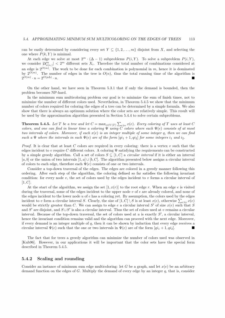
5.4. APPROXIMATING MINIMUM SUM MULTICOLORING ON THE EDGES OF TREES 113
can be easily determined by considering every set Y ⊆ {1, 2, . . . ,m} disjoint from X , and selecting theone where P (k, Y ) is minimal.
At each edge we solve at most 2m · (∆ − 1) subproblems P (i, Y ). To solve a subproblem P (i, Y ),we consider |Umx(ei)
| < 2m different sets Xi. Therefore the total number of combinations considered at
an edge is 2O(m). The work to be done for each combination is polynomial in m, hence it is dominatedby 2O(m). The number of edges in the tree is O(n), thus the total running time of the algorithm is2O(m) · n = 2O(p∆) · n. �
On the other hand, we have seen in Theorem 5.3.1 that if only the demand is bounded, then theproblem becomes NP-hard.
In the minimum sum multicoloring problem our goal is to minimize the sum of finish times, not tominimize the number of different colors used. Nevertheless, in Theorem 5.4.5 we show that the minimumnumber of colors required for coloring the edges of a tree can be determined by a simple formula. We alsoshow that there is always an optimum solution where the color sets are relatively simple. This result willbe used by the approximation algorithm presented in Section 5.4.4 to solve certain subproblems.
Theorem 5.4.5. Let T be a tree and let C = maxv∈V (T )
∑e∋v x(e). Every coloring of T uses at least C
colors, and one can find in linear time a coloring Ψ using C colors where each Ψ(e) consists of at mosttwo intervals of colors. Moreover, if each x(e) is an integer multiple of some integer q, then we can findsuch a Ψ where the intervals in each Ψ(e) are of the form [qi1 + 1, qi2] for some integers i1 and i2.
Proof. It is clear that at least C colors are required in every coloring: there is a vertex v such that theedges incident to v require C different colors. A coloring Ψ satisfying the requirements can be constructedby a simple greedy algorithm. Call a set of colors S ⊆ [1, C] a circular interval if it is either an interval[a, b] or the union of two intervals [1, a]∪ [b, C]. The algorithm presented below assigns a circular intervalof colors to each edge, therefore each Ψ(e) consists of one or two intervals.
Consider a top-down traversal of the edges. The edges are colored in a greedy manner following thisordering. After each step of the algorithm, the coloring defined so far satisfies the following invariantcondition: for every node v, the set of colors used by the edges incident to v forms a circular interval of[1, C].
At the start of the algorithm, we assign the set [1, x(r)] to the root edge r. When an edge e is visitedduring the traversal, some of the edges incident to the upper node v of e are already colored, and none ofthe edges incident to the lower node u of e has a coloring yet. By assumption, the colors used by the edgesincident to v form a circular interval S. Clearly, the size of [1, C] \ S is at least x(e), otherwise
∑e∋v x(e)
would be strictly greater than C. We can assign to edge e a circular interval S′ of size x(e) such that Sand S′ are disjoint, and S∪S′ is also a circular interval. Thus the set of colors used at v remains a circularinterval. Because of the top-down traversal, the set of colors used at u is exactly S′, a circular interval,hence the invariant condition remains valid and the algorithm can proceed with the next edge. Moreover,if every demand is an integer multiple of q, then it can be shown by induction that every edge receives acircular interval Ψ(e) such that the one or two intervals in Ψ(e) are of the form [qi1 + 1, qi2]. �
The fact that for trees a greedy algorithm can minimize the number of colors used was observed in[Kub96]. However, in our applications it will be important that the color sets have the special formdescribed in Theorem 5.4.5.
5.4.2 Scaling and rounding
Consider an instance of minimum sum edge multicoloring: let G be a graph, and let x(e) be an arbitrarydemand function on the edges of G. Multiply the demand of every edge by an integer q, that is, consider
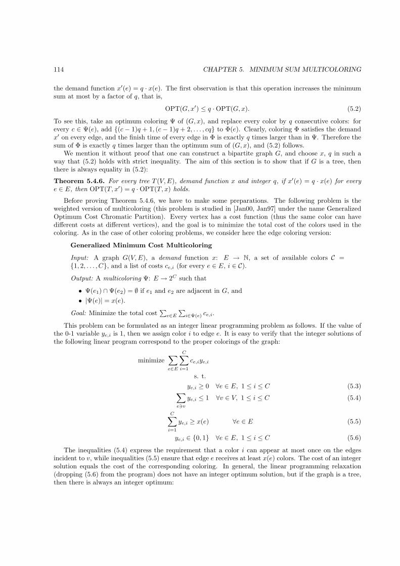
114 CHAPTER 5. MINIMUM SUM MULTICOLORING
the demand function x′(e) = q · x(e). The first observation is that this operation increases the minimumsum at most by a factor of q, that is,
OPT(G, x′) ≤ q · OPT(G, x). (5.2)
To see this, take an optimum coloring Ψ of (G, x), and replace every color by q consecutive colors: forevery c ∈ Ψ(e), add {(c− 1)q + 1, (c− 1)q + 2, . . . , cq} to Φ(e). Clearly, coloring Φ satisfies the demandx′ on every edge, and the finish time of every edge in Φ is exactly q times larger than in Ψ. Therefore thesum of Φ is exactly q times larger than the optimum sum of (G, x), and (5.2) follows.
We mention it without proof that one can construct a bipartite graph G, and choose x, q in such away that (5.2) holds with strict inequality. The aim of this section is to show that if G is a tree, thenthere is always equality in (5.2):
Theorem 5.4.6. For every tree T (V,E), demand function x and integer q, if x′(e) = q · x(e) for everye ∈ E, then OPT(T, x′) = q · OPT(T, x) holds.
Before proving Theorem 5.4.6, we have to make some preparations. The following problem is theweighted version of multicoloring (this problem is studied in [Jan00, Jan97] under the name GeneralizedOptimum Cost Chromatic Partition). Every vertex has a cost function (thus the same color can havedifferent costs at different vertices), and the goal is to minimize the total cost of the colors used in thecoloring. As in the case of other coloring problems, we consider here the edge coloring version:
Generalized Minimum Cost Multicoloring
Input: A graph G(V,E), a demand function x: E → N, a set of available colors C ={1, 2, . . . , C}, and a list of costs ce,i (for every e ∈ E, i ∈ C).
Output: A multicoloring Ψ: E → 2C such that
• Ψ(e1) ∩ Ψ(e2) = ∅ if e1 and e2 are adjacent in G, and
• |Ψ(e)| = x(e).
Goal: Minimize the total cost∑e∈E
∑i∈Ψ(e) ce,i.
This problem can be formulated as an integer linear programming problem as follows. If the value ofthe 0-1 variable ye,i is 1, then we assign color i to edge e. It is easy to verify that the integer solutions ofthe following linear program correspond to the proper colorings of the graph:
minimize∑
e∈E
C∑
i=1
ce,iye,i
s. t.
ye,i ≥ 0 ∀e ∈ E, 1 ≤ i ≤ C (5.3)∑
e∋v
ye,i ≤ 1 ∀v ∈ V, 1 ≤ i ≤ C (5.4)
C∑
i=1
ye,i ≥ x(e) ∀e ∈ E (5.5)
ye,i ∈ {0, 1} ∀e ∈ E, 1 ≤ i ≤ C (5.6)
The inequalities (5.4) express the requirement that a color i can appear at most once on the edgesincident to v, while inequalities (5.5) ensure that edge e receives at least x(e) colors. The cost of an integersolution equals the cost of the corresponding coloring. In general, the linear programming relaxation(dropping (5.6) from the program) does not have an integer optimum solution, but if the graph is a tree,then there is always an integer optimum:
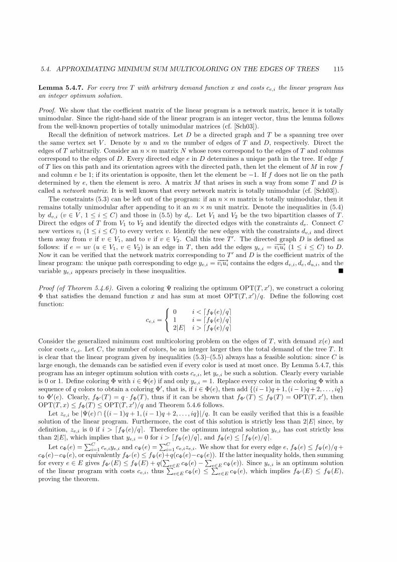
5.4. APPROXIMATING MINIMUM SUM MULTICOLORING ON THE EDGES OF TREES 115
Lemma 5.4.7. For every tree T with arbitrary demand function x and costs ce,i the linear program hasan integer optimum solution.
Proof. We show that the coefficient matrix of the linear program is a network matrix, hence it is totallyunimodular. Since the right-hand side of the linear program is an integer vector, thus the lemma followsfrom the well-known properties of totally unimodular matrices (cf. [Sch03]).
Recall the definition of network matrices. Let D be a directed graph and T be a spanning tree overthe same vertex set V . Denote by n and m the number of edges of T and D, respectively. Direct theedges of T arbitrarily. Consider an n×m matrix N whose rows correspond to the edges of T and columnscorrespond to the edges of D. Every directed edge e in D determines a unique path in the tree. If edge fof T lies on this path and its orientation agrees with the directed path, then let the element of M in row fand column e be 1; if its orientation is opposite, then let the element be −1. If f does not lie on the pathdetermined by e, then the element is zero. A matrix M that arises in such a way from some T and D iscalled a network matrix. It is well known that every network matrix is totally unimodular (cf. [Sch03]).
The constraints (5.3) can be left out of the program: if an n×m matrix is totally unimodular, then itremains totally unimodular after appending to it an m×m unit matrix. Denote the inequalities in (5.4)by dv,i (v ∈ V , 1 ≤ i ≤ C) and those in (5.5) by de. Let V1 and V2 be the two bipartition classes of T .Direct the edges of T from V1 to V2 and identify the directed edges with the constraints de. Connect Cnew vertices vi (1 ≤ i ≤ C) to every vertex v. Identify the new edges with the constraints dv,i and directthem away from v if v ∈ V1, and to v if v ∈ V2. Call this tree T ′. The directed graph D is defined asfollows: if e = uv (u ∈ V1, v ∈ V2) is an edge in T , then add the edges ye,i = −−→viui (1 ≤ i ≤ C) to D.Now it can be verified that the network matrix corresponding to T ′ and D is the coefficient matrix of thelinear program: the unique path corresponding to edge ye,i = −−→viui contains the edges dv,i, de, du,i, and thevariable ye,i appears precisely in these inequalities. �
Proof (of Theorem 5.4.6). Given a coloring Ψ realizing the optimum OPT(T, x′), we construct a coloringΦ that satisfies the demand function x and has sum at most OPT(T, x′)/q. Define the following costfunction:
ce,i =
0 i < ⌈fΨ(e)/q⌉1 i = ⌈fΨ(e)/q⌉2|E| i > ⌈fΨ(e)/q⌉
Consider the generalized minimum cost multicoloring problem on the edges of T , with demand x(e) andcolor costs ce,i. Let C, the number of colors, be an integer larger then the total demand of the tree T . Itis clear that the linear program given by inequalities (5.3)–(5.5) always has a feasible solution: since C islarge enough, the demands can be satisfied even if every color is used at most once. By Lemma 5.4.7, thisprogram has an integer optimum solution with costs ce,i, let ye,i be such a solution. Clearly every variableis 0 or 1. Define coloring Φ with i ∈ Φ(e) if and only ye,i = 1. Replace every color in the coloring Φ with asequence of q colors to obtain a coloring Φ′, that is, if i ∈ Φ(e), then add {(i− 1)q+ 1, (i− 1)q+ 2, . . . , iq}to Φ′(e). Clearly, fΦ′(T ) = q · fΦ(T ), thus if it can be shown that fΦ′(T ) ≤ fΨ(T ) = OPT(T, x′), thenOPT(T, x) ≤ fΦ(T ) ≤ OPT(T, x′)/q and Theorem 5.4.6 follows.
Let ze,i be |Ψ(e) ∩ {(i− 1)q + 1, (i− 1)q + 2, . . . , iq}|/q. It can be easily verified that this is a feasiblesolution of the linear program. Furthermore, the cost of this solution is strictly less than 2|E| since, bydefinition, ze,i is 0 if i > ⌈fΨ(e)/q⌉. Therefore the optimum integral solution ye,i has cost strictly lessthan 2|E|, which implies that ye,i = 0 for i > ⌈fΨ(e)/q⌉, and fΦ(e) ≤ ⌈fΨ(e)/q⌉.
Let cΦ(e) =∑C
i=1 ce,iye,i and cΨ(e) =∑Ci=1 ce,ize,i. We show that for every edge e, fΦ(e) ≤ fΨ(e)/q+
cΦ(e)−cΨ(e), or equivalently fΦ′(e) ≤ fΨ(e)+q(cΦ(e)−cΨ(e)). If the latter inequality holds, then summingfor every e ∈ E gives fΦ′(E) ≤ fΨ(E) + q(
∑e∈E cΦ(e) −
∑e∈E cΨ(e)). Since ye,i is an optimum solution
of the linear program with costs ce,i, thus∑
e∈E cΦ(e) ≤∑
e∈E cΨ(e), which implies fΦ′(E) ≤ fΨ(E),proving the theorem.
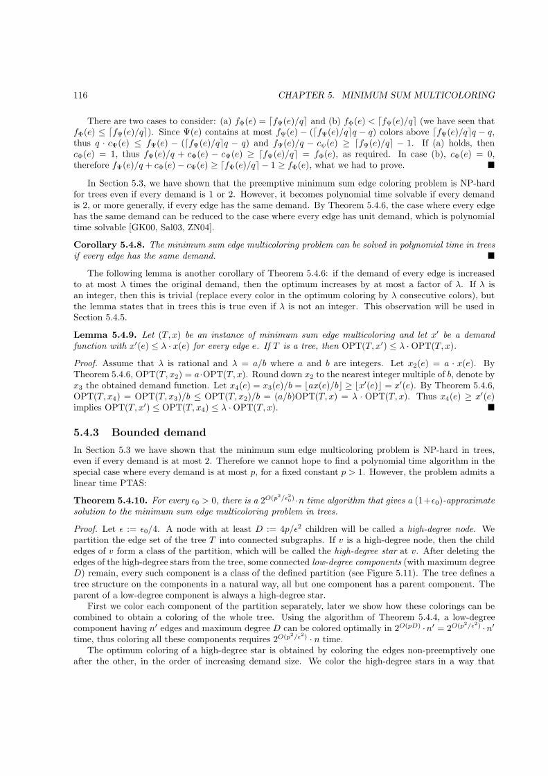
116 CHAPTER 5. MINIMUM SUM MULTICOLORING
There are two cases to consider: (a) fΦ(e) = ⌈fΨ(e)/q⌉ and (b) fΦ(e) < ⌈fΨ(e)/q⌉ (we have seen thatfΦ(e) ≤ ⌈fΨ(e)/q⌉). Since Ψ(e) contains at most fΨ(e) − (⌈fΨ(e)/q⌉q − q) colors above ⌈fΨ(e)/q⌉q − q,thus q · cΨ(e) ≤ fΨ(e) − (⌈fΨ(e)/q⌉q − q) and fΨ(e)/q − cψ(e) ≥ ⌈fΨ(e)/q⌉ − 1. If (a) holds, thencΦ(e) = 1, thus fΨ(e)/q + cΦ(e) − cΨ(e) ≥ ⌈fΨ(e)/q⌉ = fΦ(e), as required. In case (b), cΦ(e) = 0,therefore fΨ(e)/q + cΦ(e) − cΨ(e) ≥ ⌈fΨ(e)/q⌉ − 1 ≥ fΦ(e), what we had to prove. �
In Section 5.3, we have shown that the preemptive minimum sum edge coloring problem is NP-hardfor trees even if every demand is 1 or 2. However, it becomes polynomial time solvable if every demandis 2, or more generally, if every edge has the same demand. By Theorem 5.4.6, the case where every edgehas the same demand can be reduced to the case where every edge has unit demand, which is polynomialtime solvable [GK00, Sal03, ZN04].
Corollary 5.4.8. The minimum sum edge multicoloring problem can be solved in polynomial time in treesif every edge has the same demand. �
The following lemma is another corollary of Theorem 5.4.6: if the demand of every edge is increasedto at most λ times the original demand, then the optimum increases by at most a factor of λ. If λ isan integer, then this is trivial (replace every color in the optimum coloring by λ consecutive colors), butthe lemma states that in trees this is true even if λ is not an integer. This observation will be used inSection 5.4.5.
Lemma 5.4.9. Let (T, x) be an instance of minimum sum edge multicoloring and let x′ be a demandfunction with x′(e) ≤ λ · x(e) for every edge e. If T is a tree, then OPT(T, x′) ≤ λ · OPT(T, x).
Proof. Assume that λ is rational and λ = a/b where a and b are integers. Let x2(e) = a · x(e). ByTheorem 5.4.6, OPT(T, x2) = a·OPT(T, x). Round down x2 to the nearest integer multiple of b, denote byx3 the obtained demand function. Let x4(e) = x3(e)/b = ⌊ax(e)/b⌋ ≥ ⌊x′(e)⌋ = x′(e). By Theorem 5.4.6,OPT(T, x4) = OPT(T, x3)/b ≤ OPT(T, x2)/b = (a/b)OPT(T, x) = λ · OPT(T, x). Thus x4(e) ≥ x′(e)implies OPT(T, x′) ≤ OPT(T, x4) ≤ λ · OPT(T, x). �
5.4.3 Bounded demand
In Section 5.3 we have shown that the minimum sum edge multicoloring problem is NP-hard in trees,even if every demand is at most 2. Therefore we cannot hope to find a polynomial time algorithm in thespecial case where every demand is at most p, for a fixed constant p > 1. However, the problem admits alinear time PTAS:
Theorem 5.4.10. For every ǫ0 > 0, there is a 2O(p2/ǫ20) ·n time algorithm that gives a (1+ǫ0)-approximatesolution to the minimum sum edge multicoloring problem in trees.
Proof. Let ǫ := ǫ0/4. A node with at least D := 4p/ǫ2 children will be called a high-degree node. Wepartition the edge set of the tree T into connected subgraphs. If v is a high-degree node, then the childedges of v form a class of the partition, which will be called the high-degree star at v. After deleting theedges of the high-degree stars from the tree, some connected low-degree components (with maximum degreeD) remain, every such component is a class of the defined partition (see Figure 5.11). The tree defines atree structure on the components in a natural way, all but one component has a parent component. Theparent of a low-degree component is always a high-degree star.
First we color each component of the partition separately, later we show how these colorings can becombined to obtain a coloring of the whole tree. Using the algorithm of Theorem 5.4.4, a low-degreecomponent having n′ edges and maximum degree D can be colored optimally in 2O(pD) ·n′ = 2O(p2/ǫ2) ·n′
time, thus coloring all these components requires 2O(p2/ǫ2) · n time.The optimum coloring of a high-degree star is obtained by coloring the edges non-preemptively one
after the other, in the order of increasing demand size. We color the high-degree stars in a way that
5.4. APPROXIMATING MINIMUM SUM MULTICOLORING ON THE EDGES OF TREES 117
Figure 5.11: Partitioning the tree into high-degree stars (shaded regions) and low-degree components(D = 4).
is slightly worse than this optimum coloring. Assume that the parent component of the star Sv at valready has a coloring, this coloring assigns a set of colors to the edge e that connects v to its parent. Wecolor the edges in the star using only colors greater than B := p/ǫ. The edges are colored in the orderof increasing demand size, starting with the color B + 1, skipping the (at most p) colors used by e, ifnecessary. Compared to the optimum coloring given above, the finish time of every edge in the star isdelayed by at most B+p. Therefore if v has d children, then the sum of the star in this coloring is greaterthan the optimum by at most d(B + p) = d(p/ǫ + p) = dp(1/ǫ + 1) ≤ 2dp/ǫ ≤ dDǫ/2 ≤ ǫd2/2. On the
other hand, the sum of these d edges is at least∑di=1 i > d2/2 in every optimum coloring. Therefore,
ǫ · OPT(Sv) ≥ ǫd2/2
and the sum of the coloring given to Sv is not greater than (1 + ǫ)OPT(Sv).
Putting together the colorings of the components, we obtain a coloring Ψ, which is not necessarilya proper coloring: there might be conflicts between a low-degree component and its parent component,a high-degree star. The second phase of the algorithm resolves these conflicts with only a 1 + ǫ factorincrease in the total sum. First we modify the coloring Ψ such that every color greater than B is shiftedup by p. This increases by p the finish time of those edges that have finish time greater than B, andleaves the edges with finish time at most B unchanged. Therefore the finish time of every node is at most(B + p)/B ≤ 1 + ǫ times the original.
Assume that e = vu is an edge in the high-degree star at v that conflicts with some of the edgesincident to u, the lower node of e. The conflict will be solved the following way: instead of using the (atmost p) colors assigned to e, the child edges of e will use the p colors {B + 1, . . . , B + p} (in any order).This will not increase the finish time of any of the edges since the colors used by e, and therefore theconflicting colors, are all greater than B + p. To see that this modification does not introduce additionalconflicts, notice first that conflicts can appear only between edges that received new colors, since the colors{B+ 1, . . . , B+ p} were not used by any of the edges. Every recolored edge is in a low-degree component,and its parent edge is in a high-degree star. Therefore if two recolored edge are adjacent, then they havea common parent edge e. But this means that there cannot be conflict between the two edges, since everycolor in {B + 1, . . . , B + p} was given to at most one child of e.
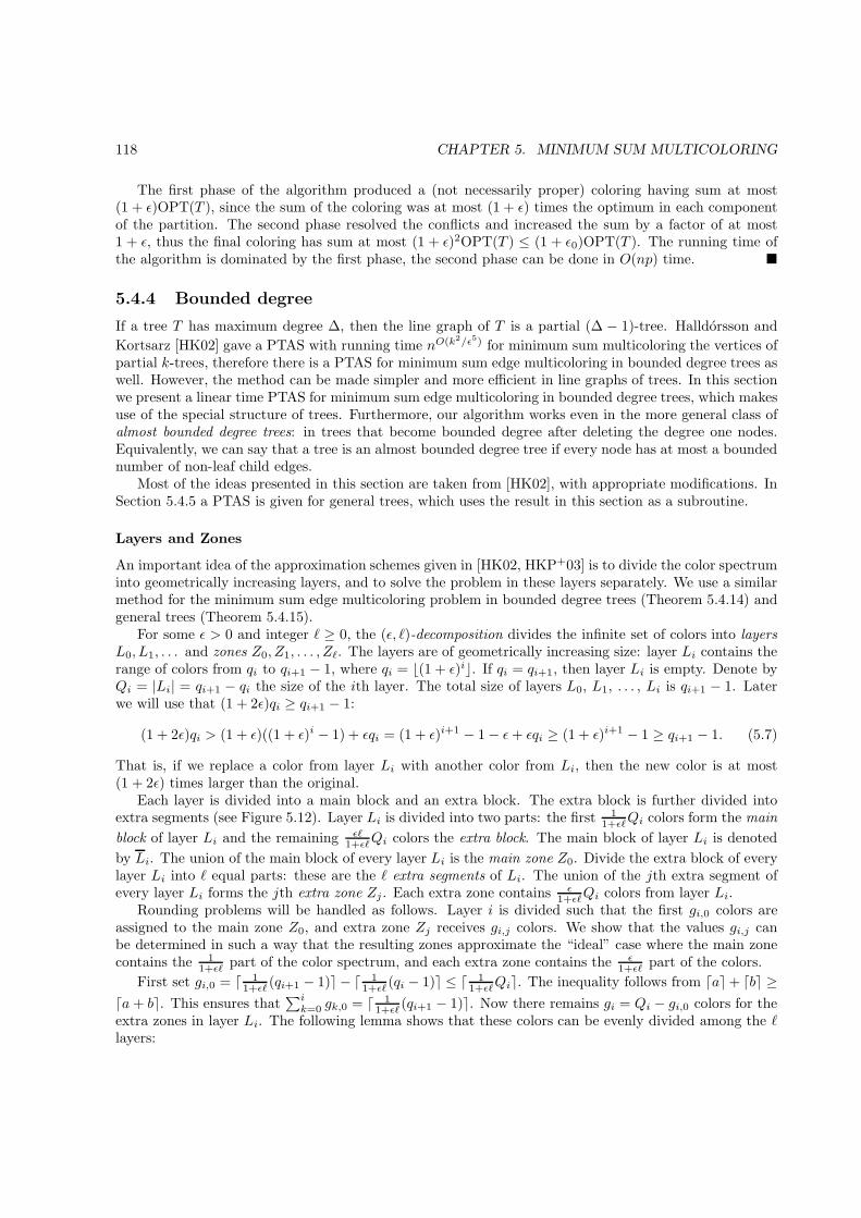
118 CHAPTER 5. MINIMUM SUM MULTICOLORING
The first phase of the algorithm produced a (not necessarily proper) coloring having sum at most(1 + ǫ)OPT(T ), since the sum of the coloring was at most (1 + ǫ) times the optimum in each componentof the partition. The second phase resolved the conflicts and increased the sum by a factor of at most1 + ǫ, thus the final coloring has sum at most (1 + ǫ)2OPT(T ) ≤ (1 + ǫ0)OPT(T ). The running time ofthe algorithm is dominated by the first phase, the second phase can be done in O(np) time. �
5.4.4 Bounded degree
If a tree T has maximum degree ∆, then the line graph of T is a partial (∆ − 1)-tree. Halldorsson and
Kortsarz [HK02] gave a PTAS with running time nO(k2/ǫ5) for minimum sum multicoloring the vertices ofpartial k-trees, therefore there is a PTAS for minimum sum edge multicoloring in bounded degree trees aswell. However, the method can be made simpler and more efficient in line graphs of trees. In this sectionwe present a linear time PTAS for minimum sum edge multicoloring in bounded degree trees, which makesuse of the special structure of trees. Furthermore, our algorithm works even in the more general class ofalmost bounded degree trees: in trees that become bounded degree after deleting the degree one nodes.Equivalently, we can say that a tree is an almost bounded degree tree if every node has at most a boundednumber of non-leaf child edges.
Most of the ideas presented in this section are taken from [HK02], with appropriate modifications. InSection 5.4.5 a PTAS is given for general trees, which uses the result in this section as a subroutine.
Layers and Zones
An important idea of the approximation schemes given in [HK02, HKP+03] is to divide the color spectruminto geometrically increasing layers, and to solve the problem in these layers separately. We use a similarmethod for the minimum sum edge multicoloring problem in bounded degree trees (Theorem 5.4.14) andgeneral trees (Theorem 5.4.15).
For some ǫ > 0 and integer ℓ ≥ 0, the (ǫ, ℓ)-decomposition divides the infinite set of colors into layersL0, L1, . . . and zones Z0, Z1, . . . , Zℓ. The layers are of geometrically increasing size: layer Li contains therange of colors from qi to qi+1 − 1, where qi = ⌊(1 + ǫ)i⌋. If qi = qi+1, then layer Li is empty. Denote byQi = |Li| = qi+1 − qi the size of the ith layer. The total size of layers L0, L1, . . . , Li is qi+1 − 1. Laterwe will use that (1 + 2ǫ)qi ≥ qi+1 − 1:
(1 + 2ǫ)qi > (1 + ǫ)((1 + ǫ)i − 1) + ǫqi = (1 + ǫ)i+1 − 1 − ǫ+ ǫqi ≥ (1 + ǫ)i+1 − 1 ≥ qi+1 − 1. (5.7)
That is, if we replace a color from layer Li with another color from Li, then the new color is at most(1 + 2ǫ) times larger than the original.
Each layer is divided into a main block and an extra block. The extra block is further divided intoextra segments (see Figure 5.12). Layer Li is divided into two parts: the first 1
1+ǫℓQi colors form the main
block of layer Li and the remaining ǫℓ1+ǫℓQi colors the extra block. The main block of layer Li is denoted
by Li. The union of the main block of every layer Li is the main zone Z0. Divide the extra block of everylayer Li into ℓ equal parts: these are the ℓ extra segments of Li. The union of the jth extra segment ofevery layer Li forms the jth extra zone Zj . Each extra zone contains ǫ
1+ǫℓQi colors from layer Li.Rounding problems will be handled as follows. Layer i is divided such that the first gi,0 colors are
assigned to the main zone Z0, and extra zone Zj receives gi,j colors. We show that the values gi,j canbe determined in such a way that the resulting zones approximate the “ideal” case where the main zonecontains the 1
1+ǫℓ part of the color spectrum, and each extra zone contains the ǫ1+ǫℓ part of the colors.
First set gi,0 = ⌈ 11+ǫℓ (qi+1 − 1)⌉ − ⌈ 1
1+ǫℓ(qi − 1)⌉ ≤ ⌈ 11+ǫℓQi⌉. The inequality follows from ⌈a⌉ + ⌈b⌉ ≥
⌈a+ b⌉. This ensures that∑i
k=0 gk,0 = ⌈ 11+ǫℓ(qi+1 − 1)⌉. Now there remains gi = Qi − gi,0 colors for the
extra zones in layer Li. The following lemma shows that these colors can be evenly divided among the ℓlayers:
5.4. APPROXIMATING MINIMUM SUM MULTICOLORING ON THE EDGES OF TREES 119
Extra segments
L0 L1 L2 L3 L4
L1 L2 L3 L4L0
Main zone Z0
Extra zone Z2
Figure 5.12: The decomposition of the colors into layers (ℓ = 3)
Lemma 5.4.11. If ℓ and gi (0 ≤ i ≤ n) are nonnegative integers, then there are nonnegative integers gi,j(0 ≤ i ≤ n, 1 ≤ j ≤ ℓ) such that for every i and j
i∑
k=0
gk,j ≥
⌊1
ℓ
i∑
k=0
gk
⌋(5.8)
andℓ∑
j=1
gi,j ≤ gi (5.9)
hold. Moreover, if∑i
k=0 gk can be calculated with a constant number of arithmetic operations, then eachgi,j can be also calculated with a constant number of arithmetic operations.
Proof. We calculate gi,j by determining the values Gi,j =∑ik=0 gk,j , then gi,j can be obtained as gi,j =
Gi,j −Gi−1,j . Let
Gi,j =
{⌈ 1ℓ
∑ik=0 gk⌉ if j ≤
∑ik=0 gk − ℓ⌊ 1
ℓ
∑ik=0 gk⌋,
⌊ 1ℓ
∑ik=0 gk⌋ otherwise.
Clearly,∑ℓj=1Gi,j =
∑ik=0 gk. It is clear that (5.8) holds, since Gi,j ≥ ⌊ 1
ℓ
∑ik=0 gk⌋. Furthermore, (5.9)
also holds:ℓ∑
j=1
gi,j =
ℓ∑
j=1
(Gi,j −Gi−1,j) =
i∑
k=0
gk −i−1∑
k=0
gk = gi.
Each Gi,j can be calculated from∑ik=0 gk by a constant number of arithmetic operations, and this is
true also for gi,j = Gi,j −Gi−1,j , hence the claim of the lemma follows. �
We will need the following properties of the defined zones:
Lemma 5.4.12. For given ℓ and ǫ ≤ 12ℓ , one can calculate values gi,j such that the resulting (ǫ, ℓ)-
decomposition of the colors has the following properties:
(a) For every c ≥ 1, zone Z0 contains at least c colors not greater than ⌊(1 + ǫℓ)c⌋.
(b) For every c ≥ 1 and 1 ≤ j ≤ ℓ, zone Zj contains at least c colors not greater than 2/ǫ · c.
Moreover, each value gi,j can be calculated using a constant number of arithmetic operations.

120 CHAPTER 5. MINIMUM SUM MULTICOLORING
Proof. Consider the values gi,j given by Lemma 5.4.11. To verify property (a), notice that for every d ≥ 1,there are at least ⌈ 1
1+ǫℓd⌉ colors in the main zone not greater than d. Indeed, if d = qi+1 − 1 (d is the lastcolor of layer Li), then this follows from the way gi,0 was defined, otherwise it follows from the fact thatthe main zone uses the first gi,0 colors of layer Li, hence if it is true for d = qi − 1 and d = qi+1 − 1, thenit is true for every value in between. Thus there are at least ⌈ 1
1+ǫℓ⌊(1 + ǫℓ)c⌋⌉ ≥ c colors below ⌊(1 + ǫℓ)c⌋.To verify property (b), assume that qi − 1 < (1 + ǫℓ)/ǫ · c ≤ qi+1 − 1 for some i. Since (1 + ǫℓ)/ǫ · c
is greater than 1/ǫ, hence (1 + 2ǫ)(1 + ǫℓ)/ǫ · c ≥ (1 + ǫℓ)/ǫ · c + 2 ≥ qi + 1 > (1 + ǫ)i. Multiplying by1 + ǫ we get (1 + ǫ)(1 + 2ǫ)(1 + ǫℓ)/ǫ · c ≥ (1 + ǫ)i+1 > qi+1 − 1. If ǫ ≤ 1
2ℓ is sufficiently small, thenqi+1 − 1 ≤ 2/ǫ · c follows. We use Lemma 5.4.11 to calculate the number of colors in the first i layers (i.e.,up to color qi+1 − 1) that belong to zone Zj :
i∑
k=0
gk,j ≥
⌊1
ℓ
i∑
k=0
gk
⌋=
⌊1
ℓ
i∑
k=0
(Qk − gk,0)
⌋=
⌊1
ℓ
(i∑
k=0
Qk −
⌈i∑
k=0
1
1 + ǫℓQk
⌉)⌋
=
⌊1
ℓ
⌊i∑
k=0
ǫℓ
1 + ǫℓQk
⌋⌋≥
⌊1
ℓ· ℓ
⌊i∑
k=0
ǫ
1 + ǫℓQk
⌋⌋=
⌊i∑
k=0
ǫ
1 + ǫℓQk
⌋
=
⌊ǫ
1 + ǫℓ(qi+1 − 1)
⌋≥
⌊ǫ
1 + ǫℓ· (1 + ǫℓ)/ǫ · c
⌋= c
Therefore there are at least c colors in zone Zj not greater than qi+1−1 ≤ 2/ǫ ·c, proving property (b). �
Given a multicoloring Ψ, the operation (ǫ, ℓ)-augmentation creates a multicoloring Φ as follows. Con-sider the (ǫ, ℓ)-decomposition of the colors, and if Ψ(e) contains color c, then let Φ(e) contain insteadthe cth color from the main zone Z0. By Lemma 5.4.12a, fΦ(e) ≤ ⌊(1 + ǫℓ)fΨ(e)⌋, thus this operationincreases the sum by at most a factor of (1 + ǫℓ). In Φ only the colors of the main zone are used.
PTAS for Bounded Degree Trees
The polynomial time algorithm of Theorem 5.4.4 was based on the observation that we have to consideronly a constant number of different colorings at each edge if both the demand and the maximum degreeare bounded. In general, however, the number of different color sets that can be assigned to an edge isexponentional in the demand. The main idea of the PTAS in [HK02] for vertex coloring partial k-trees isthat one can select a polynomial number of color sets for each vertex in such a way that there is a goodapproximate coloring using only these sets. This gives a PTAS since the best coloring that uses only theselected sets can be found in polynomial time with standard dynamic programming techniques.
Here we also follow this path: Lemma 5.4.13 shows that one can find a good approximate coloring byconsidering only a constant number of different color sets at each edge. This results in a linear time PTASfor the problem.
Lemma 5.4.13. For ǫ > 0, define bi,j = qi+j⌈ǫ2Qi/8⌉. If each vertex of the tree T has at most D non-leafchild edges and ǫ ≤ 1
3D , then it has a (1 + 3Dǫ)-approximate coloring Ψ with the following properties:
1. In the (ǫ,D)-decomposition of the colors, if e is a non-leaf edge, then Ψ(e) contains colors from themain zone only between ǫx(e)/4 and 2x(e)/ǫ.
2. If e is a non-leaf edge of type k, then Ψ(e) contains the first te colors from extra zone Zk (for somete), and it does not contain colors from the other extra zones.
3. If e is a leaf edge, then Ψ(e) contains colors only from the main zone.
4. If e is a non-leaf edge, then Ψ(e) contains at most two continuous intervals of colors from the mainblock of each layer, and the intervals in layer Li are of the form [bi,j1 , bi,j2 − 1] for some j1 and j2.
5.4. APPROXIMATING MINIMUM SUM MULTICOLORING ON THE EDGES OF TREES 121
Proof. Let Φ be an optimum solution, and let Ψ be the result of an (ǫ,D + 1)-augmentation on Φ. ByLemma 5.4.12a, fΨ(e) ≤ (1 + (D + 1)ǫ)fΦ(e) for every e (note that we assumed ǫ ≤ 1
3D < 12(D+1) ).
If fΨ(e) > 2x(e)/ǫ for a non-leaf edge e of type j, then modify Ψ(e) to be the first x(e) colors of zoneZj . By Lemma 5.4.12b, Zj contains at least x(e) colors not greater than 2x(e)/ǫ. Therefore the x(e) colorsassigned to e are not greater than 2x(e)/ǫ, hence fΨ(e) ≤ (1 + (D + 1)ǫ)fΦ(e). In this case requirements2 and 4 are automatically satisfied for e, thus there is nothing else to do with this edge.
If Ψ(e) contains colors in the main zone below ǫx(e)/4, then delete these colors and let Ψ(e) containinstead the first ǫx(e)/4 colors from zone Zj . There are at least ǫx(e)/4 colors in Zi below 2/ǫ · ǫx(e)/4 =x(e)/2. Since the finish time of e is at least x(e), hence this modification does not increase the finish timeof e. Therefore Ψ satisfies the first three properties of the lemma.
Finally, we make Ψ satisfy the fourth requirement as well. For each non-leaf edge e, let xi(e) be|Ψ(e) ∩ Li| rounded down to the next integer multiple of ⌈ǫ2Qi/8⌉. If we use xi as a demand function onthe non-leaf edges of the tree, then there is multicoloring satisfying xi that uses at most |Li| colors: Ψ(e)∩Liis such a coloring. Therefore by Theorem 5.4.5, there is a multicoloring Ψi that uses at most |Li| colors,satisfies xi, and where each Ψ(e) consists of at most two intervals of the form [1 + j1⌈ǫ2Qi/8⌉, j2⌈ǫ2Qi/8⌉]for some j1, j2. Modify coloring Ψ: let Ψi determine how the colors are assigned in the main block oflayer i. Now the third requirement is satisfied, but it is possible that Ψ assigns less than x(e) colors to anedge. We can lose at most ⌈ǫ2Qi/8⌉ − 1 < ǫ2Qi/8 colors in layer i, hence we lose at most the ǫ2/8 partof each layer. Assume that the highest color of Ψ(e) is in layer Li. Since Ψ(e) contains colors only up to2x(e)/ǫ, hence the last color of layer Li is less than 2(1 + 2ǫ)x(e)/ǫ ≤ 4x(e)/ǫ (Inequality (5.7)). Thus welose only at most ǫ2/8 · 4x(e)/ǫ = ǫx(e)/2 colors. If non-leaf edge e is of type j, then we use extra zone Zjto replace the lost colors. So far, edge e uses at most ǫx(e)/2 colors from Zj (previous paragraph), hencethere is still place for at least ǫx(e)/2 colors in Zj below (1 + (D + 1)ǫ)x(e) ≤ (1 + (D + 1)ǫ)fΦ(e).
The modification in the previous paragraph can change the finish times of the non-leaf edges, but thelargest color of each edge remains in the same layer. By Inequality (5.7), (1 + 2ǫ)qi ≥ qi+1 − 1, thereforethe finish time of an edge can increase by at most a factor of (1+2ǫ). Moreover, since we modified only thenon-leaf edges, there can be conflicts between the non-leaf and the leaf edges. But that problem is easy tosolve: since the number of colors used by the non-leaf edges at vertex v from the main block of layer i doesnot increase, there are enough colors in layer i for assigning new colors to the leaf edges. After recoloringthe leaf edges, the largest color of each edge remains in the same layer, hence the finish time of each leafedge can increase by at most a factor of 1 + 2ǫ, and fΨ(e) ≤ (1 + 2ǫ)(1 + (D+ 1)ǫ)fΦ(e) ≤ (1 + 3Dǫ)fΦ(e)follows for every edge e. �
Call a coloring satisfying the requirements of Lemma 5.4.13 a standard coloring. Notice that on anon-leaf edge e only a constant number of different color sets can appear in standard colorings: the mainzone is not empty only in a constant number of layers, and in each layer the (at most two) intervalscan be placed in a constant number of different ways. More precisely, in a standard coloring edge e canuse the main zone only from layer ⌊log1+ǫ ǫx(e)/4⌋ to layer ⌈log1+ǫ 2x(e)/ǫ⌉, that is, only in at mostlog1+ǫ((2x(e)/ǫ)/(ǫx(e)/4)) + 2 = log1+ǫ 8/ǫ2 + 2 = O(1/ǫ · log 1/ǫ) layers. In each layer, the end pointsof the intervals can take only at most 8/ǫ2 different values, hence there are (8/ǫ2)2 different possibilitiesfor each of the two intervals. Therefore if we denote by Ce the different color sets that can appear in astandard coloring on non-leaf edge e, then |Ce| = ((8/ǫ2)4)O((1/ǫ)·log 1/ǫ) = 2O((1/ǫ)·log2 1/ǫ).
Theorem 5.4.14. If every edge of T (V,E) has at most D non-leaf child edges, then for every ǫ0 > 0,
there is a 2O(D2/ǫ0·log2(D/ǫ0)) ·n time algorithm that gives a (1 + ǫ0)-approximate solution to the minimum
sum edge multicoloring problem.
Proof. Set ǫ := ǫ0/3D. We use dynamic programming to find the best standard coloring: for every non-leaf edge e, and every set S ∈ Ce, we determine OPT(e, S), which is defined to be the sum of the beststandard coloring of Te, with the additional requirement that edge e receives color set S. Clearly, if all thevalues {OPT(r, S) : S ∈ Cr} are determined for the root edge r of T , then the minimum of these values is
122 CHAPTER 5. MINIMUM SUM MULTICOLORING
the sum of the best standard coloring, which is by Lemma 5.4.13 at most (1 + 3Dǫ) = (1 + ǫ0) times theminimum sum.
The values OPT(e, S) are calculated in a bottom-up traversal of the edges. Assume that e has knon-leaf child edges e1, e2, . . . , ek and ℓ leaf child edges e′1, e
′2, . . . , e
′ℓ. When OPT(e, S) is determined, the
values OPT(ei, Si) are already available for every 1 ≤ i ≤ k and Si ∈ Cei. In a standard coloring of Te
every edge ei is assigned a color set from Cei. We enumerate all the
∏ki=1 |Cei
| possibilities for these colorsets. For each combination S1 ∈ Ce1 , . . . , Sk ∈ Cek
, we check whether these sets are pairwise disjoint. Ifso, then we determine the minimum sum that a standard coloring can have with these assignments. Theminimum sum of subtree Tei
with color set Si on ei is given by OPT(ei, Si). The finish time of edge ecan be calculated from S. Now only the leaf edges e′1, . . . , e′ℓ remain to be colored. It is easy to see thatthe best thing to do is to order these leaf edges by increasing demand size, and color them one after theother, using the colors not already assigned to e, e1, . . . , ek. Therefore we can calculate the minimumsum corresponding to a choice of color sets S1 ∈ Ce1 , . . . , Sk ∈ Cek
, and we set OPT(e, S) to the minimumover all the combinations.
The algorithm solves at most∑
e∈E |Ce| = n · 2O((1/ǫ)·log2 1/ǫ) subproblems. To solve a subproblem,
at most 2O(D·(1/ǫ)·log2 1/ǫ) different combinations of the sets S1, . . . , Sk have to be considered. Each colorset can be described by O(1/ǫ · log 1/ǫ) intervals, and the time required to handle each combinationis polynomial in D and the number of intervals. Therefore the total running time of the algorithm is2O(D·1/ǫ·log2(1/ǫ)) · n = 2O(D2/ǫ0·log
2(D/ǫ0)) · n. �
5.4.5 The general case
In this section we prove that minimum sum edge multicoloring admits a PTAS for arbitrary trees. Theedges of the tree are partitioned into subtrees in such a way that each subtree is an almost boundeddegree tree (recall that in an almost bounded degree tree each node has a bounded number of non-leafchild edges). Now the algorithm presented in Section 5.4.4 can be used to obtain a good approximatecoloring for each subtree. These colorings can be merged into a coloring of the whole tree, but this coloringwill not be necessarily a proper coloring, since there might be conflicts between edges that were in differentsubtrees. However, using a series of transformations, these conflicts can be resolved with only a smallincrease of the sum.
Theorem 5.4.15. For every ǫ0 > 0, there is a 2O(1/ǫ110 ·log2(1/ǫ0)) · n time algorithm that gives a (1 +ǫ0)-approximate solution to the minimum sum edge multicoloring problem for every tree T and demandfunction x0.
Proof. Let ǫ := ǫ0/32. The algorithm consists of a series of phases. The last phase produces a propercoloring of (T, x0), and has cost at most (1 + ǫ0)OPT(T, x0). In the following we describe these phases.
Phase 1: Rounding the Demands. Let x(e) be the smallest qi that is not smaller than x0(e). Sinceqi+1 ≤ (1 + ǫ)i+1 ≤ (1 + ǫ)(qi + 1), thus x(e) ≤ (1 + ǫ)x0(e). Therefore by Lemma 5.4.9, this modificationincreases the minimum sum by at most a factor of 1 + ǫ. An edge e with demand qi will be called a classi edge (if x(e) = qi for more than one i, then take the smallest i). The class of edge e will be denoted byclass(e).
Phase 2: Partitioning the Tree. We partition the edges of the tree into connected components suchthat in every subtree the number of non-leaf child edges of a node is bounded by a constant. To obtainthis partition, the edges of the tree are divided into large edges, small edges, and frequent edges. It willbe done in such a way that every node has at most D := 6/ǫ5 large child edges. If a node has less thanD children, then its child edges are large edges. Let v be a node with at least D children, and denoteby n(v, i) the number of class i child edges of v. Let N(v) be the largest i such that n(v, i) > 0 and set
5.4. APPROXIMATING MINIMUM SUM MULTICOLORING ON THE EDGES OF TREES 123
F := 6/ǫ3. Let e be a class i child edge of v. If n(v, i) > F , then e is a frequent edge. If n(v, i) ≤ F andi ≤ N(v) − 1/ǫ2, then e is a small edge. Otherwise, if n(v, i) ≤ F and i > N(v) − 1/ǫ2, then e is a largeedge. Clearly, v can have at most F · 1/ǫ2 = 6/ǫ5 = D large child edges: for each class N(v), N(v) − 1,. . . , N(v) − 1/ǫ2 + 1, there are at most F such edges.
The tree is split at the lower node of every small and frequent edge, the connected components of theresulting forest form the classes of the partition. Another way to describe this partition: delete everysmall and large edge, make the connected components of the remaining graph the classes of the partition,and put every deleted edge into the class where its upper node belongs. Clearly, every small and frequentedge becomes a leaf edge in its subtree, thus if every node has at most D large child edges in the tree,then in every subtree each node has at most D non-leaf child edges.
Color each subtree with the algorithm of Theorem 5.4.14. This step can be done in 2O(D2/ǫ·log2(D/ǫ)) ·n = 2O(36/ǫ10·1/ǫ·log2(6/ǫ6)) · n = 2O(1/ǫ11·log2(1/ǫ)) · n time. Each coloring is a (1 + ǫ)-approximate coloringof the given subtree, thus merging these colorings yields a (not necessarily proper) coloring Ψ1 of T suchthat fΨ1(T ) ≤ (1 + ǫ)OPT (T, x). In the rest of the proof, we transform Ψ1 into a proper coloring in sucha way that the sum of the coloring does not increase too much.
Phase 3: Small Edges. Consider the (ǫ, ℓ)-augmentation of the coloring Ψ1 with ℓ := 6. This resultsin a coloring Ψ2 such that fΨ2(G) ≤ (1 + ǫℓ)fΨ1(G) (see Section 5.4.4). First we modify Ψ2 in sucha way that the small edges use only the extra zones Z1 and Z2. More precisely, if a small edge e hasparity r ∈ {1, 2}, then e is recolored using the colors in Zr (recall that the parity of the edge is the parityof its upper node). Since the extra zones contain only a very small fraction of the color spectrum, therecoloring can significantly increase the finish time of the small edges, but not more than by a factor of 2/ǫ(Lemma 5.4.12b). However, we show that the total demand of the small edges at v is so small comparedto the largest demand on the child edges of v, that their total finish time will be negligible, even after thislarge increase. By definition, the largest child edge of v has demand qN(v).
Let Sv be the set of those small edges whose upper node is v. Let r be the parity of v. Color the edgesin Sv one after the other, in the order of increasing demand size, using only the colors in Zr. Call theresulting coloring Ψ3. We claim that fΨ3(Sv) ≤ ǫqN(v) for every node v, thus transforming Ψ2 into Ψ3
increases the total sum by at most∑
v∈T fΨ3(Sv) ≤ ǫ∑v∈T qN(v) ≤ ǫfΨ2(T ) and fΨ3(T ) ≤ (1 + ǫ)fΨ2(T )
follows. To give an upper bound on fΨ3(Sv), we assume the worst case, that is, n(v, i) = F for everyi ≤ N(v) − 1/ǫ2. Imagine first that the small edges are colored using the full color spectrum, not onlywith the colors of zone Zr. Assume that the small edges are colored in the order of increasing demandsize, and consider a class k edge e. In the coloring, only edges of class not greater than k are coloredbefore e. Hence the finish time of e is at most
k∑
i=0
n(v, i)qi ≤ Fk∑
i=0
(1 + ǫ)i ≤ 6(1 + ǫ)/ǫ4 · (1 + ǫ)k
≤ 14/ǫ4 ·1
2(1 + ǫ)k ≤ 14/ǫ4 · ⌊(1 + ǫ)k⌋ = 14/ǫ4 · qk.
That is, the finish time of an edge is at most 14/ǫ4 times its demand (in the second inequality, we used∑ki=0(1 + ǫ)i = ((1 + ǫ)k+1 − 1)/ǫ < (1 + ǫ)k+1/ǫ). Therefore the total finish time of the small edges is at
most 14/ǫ4 times the total demand, which is
14
ǫ4
N(v)−1/ǫ2∑
i=0
n(v, i)qi ≤84
ǫ7
N(v)−1/ǫ2∑
i=0
(1 + ǫ)i
≤85
ǫ8(1 + ǫ)N(v)−1/ǫ2 ≤
85
ǫ8· 2−1/ǫ · (1 + ǫ)N(v)
≤ǫ2
2·
1
2(1 + ǫ)N(v) ≤
ǫ2
2· ⌊(1 + ǫ)N(v)⌋ =
ǫ2
2· qN(v).
124 CHAPTER 5. MINIMUM SUM MULTICOLORING
(In the third inequality we use (1 + ǫ)1/ǫ ≥ 2, in the fourth inequality it is assumed that ǫ is sufficientlysmall that 21/ǫ ≥ 4 · 85/ǫ10 holds.) However, the small edges do not use the full color spectrum, only thecolors in zone Zr. By Lemma 5.4.12b, zone Zr contains at least c colors up to 2/ǫ · c, thus every finishtime in the calculation above should be multiplied by at most 2/ǫ. Therefore the sum of the small edgesis at most
fΨ3(Sv) ≤ 2/ǫ ·ǫ2
2· qN(v) ≤ ǫqN(v),
as claimed.
Phase 4: Shifting the Frequent Edges. Now we have a coloring Ψ3 that is still not a proper coloring,but conflicts appear only between some frequent edges and their child edges. In Phases 4 and 5 we ensurethat every frequent edge e uses only colors greater than 2x(e)/ǫ from the main zone. In Phase 6, theconflicts are resolved using a set of so far unused colors, the colors in extra zones Z5 and Z6.
Let Fv be the set of frequent child edges of v, and let Λv =⋃e∈Fv
Ψ3(e) be the colors used by thefrequent child edges of node v. We recolor the edges in Fv using only the colors in Λv and some colorsfrom zones Z3 and Z4. Let e1, e2, . . . , e|Fv| be an ordering of the edges in Fv by increasing demand size.Recall that the algorithm in Theorem 5.4.14 assigned the colors to the leaf edges in increasing order ofdemand size, thus it can be assumed that frequent edge e1 uses the first x(e1) colors in Λv, edge e2 usesthe x(e2) colors after that, etc. Denote by t(c) = |{e ∈ Fv : fΨ3(e) ≥ c}| the number of edges whose finishtime is at least c, and denote by t(c, i) = |{e ∈ Fv : fΨ3(e) ≥ c, class(e) = i}| the number of class i edgesamong them. Clearly, t(c) =
∑∞i=0 t(c, i) holds. Moreover, it can be easily verified that the total finish
time of the edges in Fv can be expressed as fΨ3(Fv) =∑∞
c=1 t(c).The first step is to produce a coloring Ψ4 where every frequent edge e has only (1−2ǫ/5)x(e) colors, but
these colors are all greater than 2x(e)/ǫ. The demand function is split into two parts: x(e) = x1(e)+x2(e),where x1(e) is (1− 2ǫ/5)x(e) and x2(e) is 2ǫx(e)/5, but rounding has to be done carefully. What we wantto achieve is that
k∑
j=1
x2(ej) ≤2ǫ
5
k∑
j=1
x(ej) (5.10)
holds for every 1 ≤ k ≤ |Fv|, and the total demand of the class i edges in x1 is at most
∑
e∈Fv , class(e)=i
x1(e) ≤ ⌈n(e, i)(1 − 2ǫ/5)qi⌉. (5.11)
It can be easily verified that these two requirements hold if x1 is defined as x1(e) = ⌈(1− 2ǫ/5)qi⌉ for thefirst m edges of class i, and x1(e) = ⌊(1 − 2ǫ/5)qi⌋ for the rest of the class i edges, where
m = ⌈n(v, i)(1 − 2ǫ/5)qi⌉ − n(v, i) ⌊(1 − 2ǫ/5)qi⌋ .
This phase of the algorithm produces a coloring Ψ4 of Fv that assigns only x1(e) colors to every edgee ∈ Fv, but satisfies the condition that it uses only the colors in Λv, and every edge e receives only colorsgreater than 2x(e)/ǫ. In the next phase we will extend this coloring using the colors in zones Z3 and Z4:every edge e will receive an additional x2(e) colors.
Coloring Ψ4 is defined as follows. Consider the edges e1, . . . , e|Fv| in this order, and assign to ek thefirst x1(ek) colors in Λv greater than 2x(ek)/ǫ and not already assigned to an edge ej (j < k). Noticethe following property of Ψ4: if j < k, then every color in Ψ4(ej) is less than every color in Ψ4(ek).This follows from 2x(ej)/ǫ ≤ 2x(ek)/ǫ: every color usable for ek is also usable for ej if j < k. Definet′(c) = |{e ∈ Fv : fΨ4(e) ≥ c}| and t′(c, i) = |{e ∈ Fv : fΨ4(e) ≥ c, class(e) = i}| as before, but now usingthe coloring Ψ4. We claim that t′(c, i) ≤ (1 + ǫ)t(c, i) holds for every c ≥ 1, i ≥ 0. If this is true, thent′(c) ≤ (1 + ǫ)t(c) holds and fΨ4(Fv) ≤ (1 + ǫ)fΨ3(Fv) follows from fΨ4(Fv) =
∑∞c=1 t
′(c). Summing thisfor every node v gives fΨ4(T ) ≤ (1 + ǫ)fΨ3(T ).
5.4. APPROXIMATING MINIMUM SUM MULTICOLORING ON THE EDGES OF TREES 125
First we show that t′(c, i) ≤ t(c, i) + 2/ǫ. If every class i edge has finish time at least c in Ψ3, thent(c, i) = n(c, i) ≥ t′(c, i) and we are ready. Therefore there is at least one class i edge that has finish timeless than c in Ψ3. This implies that the frequent edges of class 0, 1, . . . , i − 1 use only colors less thanc. Denote by X the total demand of these edges (in the demand function x(e)), and denote by Y thenumber of colors used by the class i edges below c in Ψ3.
Now recall the way Ψ4 was defined, and consider the step when every edge with class less than i isalready colored. At this point at most X colors of Λv are used below c (possibly less, since Ψ4 assigns onlyx1(e) colors to every edge e, and only colors above 2x(e)/ǫ). Therefore at least Y colors are still unusedin Λv below c. From these colors at least Y − 2qi/ǫ of them are above 2qi/ǫ. Thus Ψ4 can color at least(Y − 2qi/ǫ)/qi = Y/qi − 2/ǫ edges of class i using only colors below c. However, Ψ3 uses Y colors below cfor the class i edges, hence it can color at most Y/qi such edges below c, and t′(c, i) ≤ t(c, i) + 2/ǫ follows.
We consider two cases. If t(c, i) ≥ 2/ǫ2, then t′(c, i) ≤ t(c, i) + 2/ǫ ≤ (1 + ǫ)t(c, i), and we are ready.Let us assume therefore that t(c, i) ≤ 2/ǫ2, it will turn out that in this case t′(c, i) = 0. There aren(v, i) − t(c, i) ≥ n(v, i) − 2/ǫ2 class i edges that has finish time less than c in Ψ3. Therefore, as in theprevious paragraph, before Ψ4 starts coloring the class i edges, there are at least (n(v, i)−2/ǫ2) ·qi unusedcolors less than c in Λv. By (5.11), the total demand of the class i edges in demand function x1(e) isat most ⌈n(e, i)(1 − 2ǫ/5)qi⌉. The following calculation shows that the unused colors below c in Λv issufficient to satisfy all these edges, thus Ψ4 assigns to these edges only colors less than c. We have to skipthe colors not greater than 2qi/ǫ, these colors cannot be assigned to the edges of class i, which means thatthe number of usable colors is at least
(n(v, i) − 2/ǫ2) · qi − 2qi/ǫ ≥ (n(v, i) − 12/5ǫ2) · qi + 1
≥ (1 − 2ǫ/5)n(v, i)qi + 1 ≥ ⌈n(e, i)(1 − 2ǫ/5)qi⌉,
since n(v, i) ≥ 6/ǫ3 by the definition of the frequent edges. Therefore Ψ4 assigns to the class i edges onlycolors less than c, and t(c, i) = 0 follows.
Phase 5: Full Demand for the Frequent Edges. The next step is to modify Ψ4 such that everyfrequent edge receives x(e) colors, not only x1(e). Coloring Ψ5 is obtained from Ψ4 by assigning to everyfrequent edge e an additional x2(e) colors from zone Z3 or Z4. More precisely, let v be a node with parityr, and let e1, . . . , e|Fv| be its frequent child edges, ordered in increasing demand size, as before. Assign toe1 the first x2(e1) colors from Z2+r, to e2 the first x2(e2) colors from Z2+r not used by e1, etc. It is clearthat no conflict arises with the assignment of these colors.
We claim that these additional colors do not increase the finish time of the frequent edges. Letx∗i =
∑ij=1 x1(ej) be the total demand in x1 of the first i frequent edges at v. The finish time of ei
in Ψ4 is clearly at least x∗i , since Ψ4 colors every edge ej with j < i before ei. On the other hand, byLemma 5.4.12b, zone Z2+r contains at least ⌊ǫx∗i /2⌋ colors not greater than x∗i . These colors are sufficientto satisfy the additional demand of the first i edges: by (5.10) the first i edges need a total of at most2ǫ5
∑ij=1 x(e) ≤ ǫx∗i /2 colors.
Phase 6: Resolving the Conflicts. Now we have a coloring Ψ5 such that there are conflicts onlybetween frequent edges and their child edges. Furthermore, if e is a frequent edge, then Ψ5(e) containsonly colors greater than 2x(e)/ǫ from the main zone. It is clear from the construction of Ψ5 that only thecolors in the main zone can conflict.
Let e be a frequent edge that conflicts with some of its children. Assume that the child edges of e haveparity r. There are at most x(e) colors that are used by both e and a child of e. We resolve this conflictby recoloring the child edges of e in such a way that they use the first at most x(e) colors in zone Z4+r
instead of the colors in Ψ5(e). It is clear that if this operation is applied for every frequent edge e, thenthe resulting color Ψ6 is a proper coloring.
126 CHAPTER 5. MINIMUM SUM MULTICOLORING
Notice that if a child edge e′ of e is recolored, then it has finish time at least 2x(e)/ǫ, otherwise itdoes not conflict with e. On the other hand, by Lemma 5.4.12b, zone Z4+r contains at least x(e) colorsup to 2x(e)/ǫ, thus the recoloring does not add colors above that. Therefore the finish time of e′ is notincreased.
Analysis. The sum of the coloring Ψ6 can be bounded as follows (assuming that ǫ is sufficiently small):
fΨ6(T ) = fΨ5(T ) = fΨ4(T ) ≤ (1 + ǫ)fΨ3(T )
≤ (1 + ǫ)2fΨ2(T ) ≤ (1 + (ℓ+ 1)ǫ)(1 + ǫ)2fΨ1(T )
≤ (1 + (ℓ+ 1)ǫ)(1 + ǫ)3OPT(T, x) ≤ (1 + (ℓ+ 1)ǫ)(1 + ǫ)4OPT(T, x0)
≤ (1 + 7ǫ)(1 + 8ǫ)OPT(T, x0) ≤ (1 + 32ǫ)OPT(T, x0)
= (1 + ǫ0)OPT(T, x0)
Therefore Ψ6 is a (1 + ǫ0)-approximate solution to the minimum sum edge multicoloring instance (T, x0).The running time of the algorithm is dominated by the coloring of the low-degree components with the
algorithm of Theorem 5.4.14. This phase requires 2O(36/ǫ10·1/ǫ·log2(6/ǫ6)) · n = 2O(1/ǫ110 log2(1/ǫ0)) · n time.The other parts of the algorithm can be done in time linear in the size of the input. Therefore the totalrunning time is 2O(1/ǫ110 log2(1/ǫ0)) · n, which completes the proof of Theorem 5.4.15. �
CHAPTER 6
Clique coloring
The worst cliques are those which consist of one man.George Bernard Shaw (1856–1950)
In clique coloring we have to satisfy weaker requirements than in ordinary vertex coloring. Insteadof requiring that the two end points of each edge have two different colors, we only require that everyinclusionwise maximal (nonextendable) clique contains at least two different colors. It is possible that agraph is k-clique-colorable, but its chromatic number is greater than k. For example, a clique of size n is2-clique-colorable, but its chromatic number is n.
Clique coloring can be also thought of as coloring the clique hypergraph. Given a graph G(V,E), theclique hypergraph C(G) of G is defined on the same vertex set V , and a subset V ′ ⊆ V is a hyperedgeof C(G) if and only if |V ′| > 1 and V ′ induces an inclusionwise maximal clique of G. The study ofthe clique hypergraph was initiated by Gallai. Most of the research on the clique hypergraph focuseson the transversals of C(G), that is, how many vertices are required to meet all the maximal cliques[EGT92, AF96]. However, it is equally natural to study the colorings of the clique hypergraph. Coloringa hypergraph means assigning colors to the vertices in such a way that every hyperedge contains at leasttwo colors. Clearly, a graph G is k-clique-colorable if and only if the hypergraph C(G) is k-colorable. Ifthe graph G is triangle-free, then the maximal cliques are the edges, hence C(G) is the same as G.
Clique coloring can be very different from ordinary vertex coloring. The most notable difference is thatclique coloring is not a hereditary property: it is possible that a graph is k-clique-colorable, but it has asubgraph that is not. The reason why this can happen is that deleting vertices can create new inclusionwisemaximal cliques: it is possible that in the original graph a clique is contained in a larger clique, but afterdeleting some vertices this clique becomes maximal. Another difference is that a large clique is not anobstruction for clique colorability, even 2-clique-colorable graphs can contain large cliques. In fact, itis conjectured that every prefect graph (or perhaps every odd-hole free graph) is 3-clique-colorable (see[BGG+04]). There are no counterexamples known for this conjecture, but so far only some special caseshave been proved.
In this chapter we prove complexity results for clique coloring and related problems. Clique coloringis harder than ordinary vertex coloring: it is coNP-complete even to check whether a 2-clique-coloring isvalid [BGG+04]. The complexity of 2-clique-colorability is investigated in [KT02], where they show thatit is NP-hard to decide whether a perfect graph is 2-clique-colorable. However, it is not clear whether thisproblem belongs to NP. A valid 2-clique-coloring is not a good certificate, since we cannot verify it in
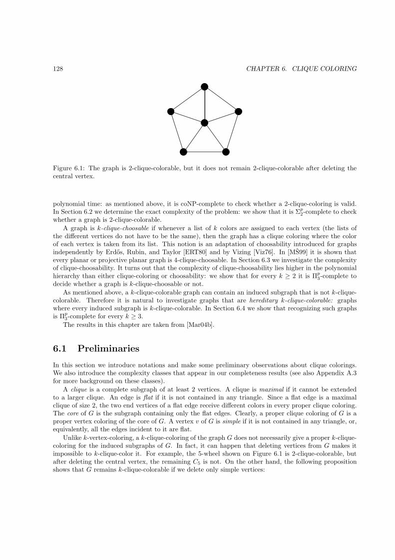
128 CHAPTER 6. CLIQUE COLORING
Figure 6.1: The graph is 2-clique-colorable, but it does not remain 2-clique-colorable after deleting thecentral vertex.
polynomial time: as mentioned above, it is coNP-complete to check whether a 2-clique-coloring is valid.In Section 6.2 we determine the exact complexity of the problem: we show that it is Σp2-complete to checkwhether a graph is 2-clique-colorable.
A graph is k-clique-choosable if whenever a list of k colors are assigned to each vertex (the lists ofthe different vertices do not have to be the same), then the graph has a clique coloring where the colorof each vertex is taken from its list. This notion is an adaptation of choosability introduced for graphsindependently by Erdos, Rubin, and Taylor [ERT80] and by Vizing [Viz76]. In [MS99] it is shown thatevery planar or projective planar graph is 4-clique-choosable. In Section 6.3 we investigate the complexityof clique-choosability. It turns out that the complexity of clique-choosability lies higher in the polynomialhierarchy than either clique-coloring or choosability: we show that for every k ≥ 2 it is Πp
3-complete todecide whether a graph is k-clique-choosable or not.
As mentioned above, a k-clique-colorable graph can contain an induced subgraph that is not k-clique-colorable. Therefore it is natural to investigate graphs that are hereditary k-clique-colorable: graphswhere every induced subgraph is k-clique-colorable. In Section 6.4 we show that recognizing such graphsis Πp
3-complete for every k ≥ 3.
The results in this chapter are taken from [Mar04b].
6.1 Preliminaries
In this section we introduce notations and make some preliminary observations about clique colorings.We also introduce the complexity classes that appear in our completeness results (see also Appendix A.3for more background on these classes).
A clique is a complete subgraph of at least 2 vertices. A clique is maximal if it cannot be extendedto a larger clique. An edge is flat if it is not contained in any triangle. Since a flat edge is a maximalclique of size 2, the two end vertices of a flat edge receive different colors in every proper clique coloring.The core of G is the subgraph containing only the flat edges. Clearly, a proper clique coloring of G is aproper vertex coloring of the core of G. A vertex v of G is simple if it is not contained in any triangle, or,equivalently, all the edges incident to it are flat.
Unlike k-vertex-coloring, a k-clique-coloring of the graph G does not necessarily give a proper k-clique-coloring for the induced subgraphs of G. In fact, it can happen that deleting vertices from G makes itimpossible to k-clique-color it. For example, the 5-wheel shown on Figure 6.1 is 2-clique-colorable, butafter deleting the central vertex, the remaining C5 is not. On the other hand, the following propositionshows that G remains k-clique-colorable if we delete only simple vertices:

6.1. PRELIMINARIES 129
Proposition 6.1.1. Let S ⊆ V be a set of simple vertices in G(V,E). If ψ is a proper clique coloring ofG, then ψ induces a proper clique coloring of G \ S.
Proof. Consider the coloring ψ′ of G \ S induced by ψ. If ψ′ is not a clique coloring of G, then there isa monochromatic maximal clique K in G \ S. This is not a maximal clique in G, otherwise ψ would notbe a proper k-clique-coloring. Therefore K is properly contained in a maximal clique K ′ of G. Since K ′
is not a maximal clique of G \ S, it contains at least one vertex v of S. However, K ′ has size at least 3,contradicting the assumption that vertex v ∈ S is simple. �
The following two propositions will also be useful:
Proposition 6.1.2. Let S ⊆ V be an arbitrary subset of the vertices in G(V,E). If ψ induces a properclique coloring of G \ S, and every vertex in S has different color from its neighbors, then ψ is a properclique coloring of G.
Proof. If there is a monochromatic maximal clique K in G, then it contains a vertex v from S. However,vertex v has different color from its neighbors, a contradiction. �
Proposition 6.1.3. Let S ⊆ V be the set of simple vertices in G(V,E). If ψ is a k-clique-coloring of G,then it induces a proper k-vertex-coloring of G[S], the graph induced by S.
Proof. Observe that every edge in G[S] is a flat edge, they are maximal cliques in G. Therefore ψ assignsdifferent colors to the end vertices of every edge in G[S], thus it induces a proper k-vertex-coloring ofG[S]. �
The complexity class Σp2 = NPNP contains those problems that can be solved by a polynomial timenondeterministic Turing machine equipped with an NP-oracle. An oracle can be thought of as a subroutinethat is capable of solving instantaneously a certain problem. More formally, let L be a language. A Turingmachine equipped with an L oracle has a special tape called the oracle tape. Whenever the Turing machinewishes, it can ask the oracle whether the contents of the oracle tape is a word from L or not (there arespecial states for this purpose). Asking the oracle counts as only one step. If the language L is simple,then this oracle does not help very much. On the other hand, if L is a computationally hard language,then this oracle can increase the power of the Turing machine. We say that a Turing machine is equippedwith an NP-oracle, if the language L is NP-complete. Note that here it is not really important whichparticular NP-complete language is L: any NP-complete language gives the same power to the Turingmachine, up to a polynomial factor. Thus the class Σp2 contains those problems that can be solved inpolynomial time by a polynomial time nondeterministic Turing machine if one NP-complete problem (say,the satisfiability problem) can be solved in constant time.
Similarly to NP, the class Σp2 has an equivalent characterization using certificates. A problem is in NPif there is a polynomial-size certificate for each yes-instance, and verifying this certificate is a problem inP. The characterization of the class Σp2 is similar, but here we require only that verifying the certificateis in coNP (cf. [Pap94] for more details).
Like SAT, which is the canonical complete problem for NP, the problem QSAT2 is the canonicalΣp2-complete problem:
2-Quantified Satisfiability (QSAT2)
Input: An n + m variable boolean 3DNF formula ϕ(x,y) (where x = (x1, . . . , xn), y =(y1, . . . , ym))
Question: Is there a vector x ∈ {0, 1}n such that for every y ∈ {0, 1}m, ϕ(x,y) is true?(Shorthand notation: is it true that ∃x∀yϕ(x,y)?)
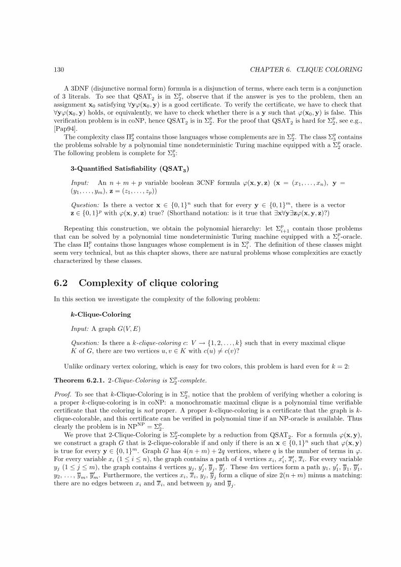
130 CHAPTER 6. CLIQUE COLORING
A 3DNF (disjunctive normal form) formula is a disjunction of terms, where each term is a conjunctionof 3 literals. To see that QSAT2 is in Σp2, observe that if the answer is yes to the problem, then anassignment x0 satisfying ∀yϕ(x0,y) is a good certificate. To verify the certificate, we have to check that∀yϕ(x0,y) holds, or equivalently, we have to check whether there is a y such that ϕ(x0,y) is false. Thisverification problem is in coNP, hence QSAT2 is in Σp2. For the proof that QSAT2 is hard for Σp2, see e.g.,[Pap94].
The complexity class Πp2 contains those languages whose complements are in Σp2. The class Σp3 contains
the problems solvable by a polynomial time nondeterministic Turing machine equipped with a Σp2 oracle.The following problem is complete for Σp3:
3-Quantified Satisfiability (QSAT3)
Input: An n + m + p variable boolean 3CNF formula ϕ(x,y, z) (x = (x1, . . . , xn), y =(y1, . . . , ym), z = (z1, . . . , zp))
Question: Is there a vector x ∈ {0, 1}n such that for every y ∈ {0, 1}m, there is a vectorz ∈ {0, 1}p with ϕ(x,y, z) true? (Shorthand notation: is it true that ∃x∀y∃zϕ(x,y, z)?)
Repeating this construction, we obtain the polynomial hierarchy: let Σpi+1 contain those problemsthat can be solved by a polynomial time nondeterministic Turing machine equipped with a Σpi -oracle.The class Πp
i contains those languages whose complement is in Σpi . The definition of these classes mightseem very technical, but as this chapter shows, there are natural problems whose complexities are exactlycharacterized by these classes.
6.2 Complexity of clique coloring
In this section we investigate the complexity of the following problem:
k-Clique-Coloring
Input: A graph G(V,E)
Question: Is there a k-clique-coloring c: V → {1, 2, . . . , k} such that in every maximal cliqueK of G, there are two vertices u, v ∈ K with c(u) 6= c(v)?
Unlike ordinary vertex coloring, which is easy for two colors, this problem is hard even for k = 2:
Theorem 6.2.1. 2-Clique-Coloring is Σp2-complete.
Proof. To see that k-Clique-Coloring is in Σp2, notice that the problem of verifying whether a coloring isa proper k-clique-coloring is in coNP: a monochromatic maximal clique is a polynomial time verifiablecertificate that the coloring is not proper. A proper k-clique-coloring is a certificate that the graph is k-clique-colorable, and this certificate can be verified in polynomial time if an NP-oracle is available. Thusclearly the problem is in NPNP = Σp2.
We prove that 2-Clique-Coloring is Σp2-complete by a reduction from QSAT2. For a formula ϕ(x,y),we construct a graph G that is 2-clique-colorable if and only if there is an x ∈ {0, 1}n such that ϕ(x,y)is true for every y ∈ {0, 1}m. Graph G has 4(n+ m) + 2q vertices, where q is the number of terms in ϕ.For every variable xi (1 ≤ i ≤ n), the graph contains a path of 4 vertices xi, x
′i, x
′i, xi. For every variable
yj (1 ≤ j ≤ m), the graph contains 4 vertices yj , y′j , yj , y
′j . These 4m vertices form a path y1, y′1, y1, y′1,
y2, . . . , ym, y′m. Furthermore, the vertices xi, xi, yj, yj form a clique of size 2(n+m) minus a matching:there are no edges between xi and xi, and between yj and yj .
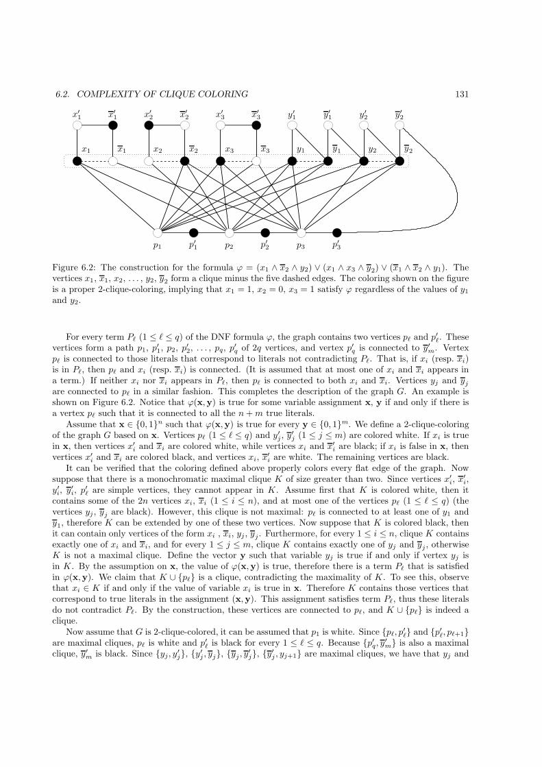
6.2. COMPLEXITY OF CLIQUE COLORING 131
p3 p′3p′2p2p′1p1
y2y2y1y1x3x3x2x2x1x1
y′2y′2y′1y′1x′3x′3x′2x′2x′1x′1
Figure 6.2: The construction for the formula ϕ = (x1 ∧ x2 ∧ y2) ∨ (x1 ∧ x3 ∧ y2) ∨ (x1 ∧ x2 ∧ y1). Thevertices x1, x1, x2, . . . , y2, y2 form a clique minus the five dashed edges. The coloring shown on the figureis a proper 2-clique-coloring, implying that x1 = 1, x2 = 0, x3 = 1 satisfy ϕ regardless of the values of y1and y2.
For every term Pℓ (1 ≤ ℓ ≤ q) of the DNF formula ϕ, the graph contains two vertices pℓ and p′ℓ. Thesevertices form a path p1, p′1, p2, p′2, . . . , pq, p
′q of 2q vertices, and vertex p′q is connected to y′m. Vertex
pℓ is connected to those literals that correspond to literals not contradicting Pℓ. That is, if xi (resp. xi)is in Pℓ, then pℓ and xi (resp. xi) is connected. (It is assumed that at most one of xi and xi appears ina term.) If neither xi nor xi appears in Pℓ, then pℓ is connected to both xi and xi. Vertices yj and yjare connected to pℓ in a similar fashion. This completes the description of the graph G. An example isshown on Figure 6.2. Notice that ϕ(x,y) is true for some variable assignment x, y if and only if there isa vertex pℓ such that it is connected to all the n+m true literals.
Assume that x ∈ {0, 1}n such that ϕ(x,y) is true for every y ∈ {0, 1}m. We define a 2-clique-coloringof the graph G based on x. Vertices pℓ (1 ≤ ℓ ≤ q) and y′j , y
′j (1 ≤ j ≤ m) are colored white. If xi is true
in x, then vertices x′i and xi are colored white, while vertices xi and x′i are black; if xi is false in x, thenvertices x′i and xi are colored black, and vertices xi, x
′i are white. The remaining vertices are black.
It can be verified that the coloring defined above properly colors every flat edge of the graph. Nowsuppose that there is a monochromatic maximal clique K of size greater than two. Since vertices x′i, x
′i,
y′i, y′i, p
′ℓ are simple vertices, they cannot appear in K. Assume first that K is colored white, then it
contains some of the 2n vertices xi, xi (1 ≤ i ≤ n), and at most one of the vertices pℓ (1 ≤ ℓ ≤ q) (thevertices yj , yj are black). However, this clique is not maximal: pℓ is connected to at least one of y1 andy1, therefore K can be extended by one of these two vertices. Now suppose that K is colored black, thenit can contain only vertices of the form xi , xi, yj , yj . Furthermore, for every 1 ≤ i ≤ n, clique K containsexactly one of xi and xi, and for every 1 ≤ j ≤ m, clique K contains exactly one of yj and yj , otherwiseK is not a maximal clique. Define the vector y such that variable yj is true if and only if vertex yj isin K. By the assumption on x, the value of ϕ(x,y) is true, therefore there is a term Pℓ that is satisfiedin ϕ(x,y). We claim that K ∪ {pℓ} is a clique, contradicting the maximality of K. To see this, observethat xi ∈ K if and only if the value of variable xi is true in x. Therefore K contains those vertices thatcorrespond to true literals in the assignment (x,y). This assignment satisfies term Pℓ, thus these literalsdo not contradict Pℓ. By the construction, these vertices are connected to pℓ, and K ∪ {pℓ} is indeed aclique.
Now assume that G is 2-clique-colored, it can be assumed that p1 is white. Since {pℓ, p′ℓ} and {p′ℓ, pℓ+1}are maximal cliques, pℓ is white and p′ℓ is black for every 1 ≤ ℓ ≤ q. Because {p′q, y
′m} is also a maximal
clique, y′m is black. Since {yj, y′j}, {y′j , yj}, {yj , y′j}, {y′j , yj+1} are maximal cliques, we have that yj and
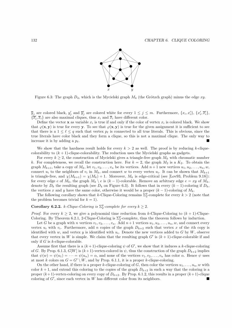
132 CHAPTER 6. CLIQUE COLORING
yx
Figure 6.3: The graph D4, which is the Mycielski graph M4 (the Grotzch graph) minus the edge xy.
yj are colored black, y′j and y′j are colored white for every 1 ≤ j ≤ m. Furthermore, {xi, x′i}, {x′i, x′i},
{x′i, xi} are also maximal cliques, thus xi and xi have different color.Define the vector x as variable xi is true if and only if the color of vertex xi is colored black. We show
that ϕ(x,y) is true for every y. To see that ϕ(x,y) is true for the given assignment it is sufficient to seethat there is a 1 ≤ ℓ ≤ q such that vertex pℓ is connected to all true literals. This is obvious, since thetrue literals have color black and they form a clique, so this is not a maximal clique. The only way toincrease it is by adding a pℓ. �
We show that the hardness result holds for every k > 2 as well. The proof is by reducing k-clique-colorability to (k + 1)-clique-colorability. The reduction uses the Mycielski graphs as gadgets.
For every k ≥ 2, the construction of Mycielski gives a triangle-free graph Mk with chromatic numberk. For completeness, we recall the construction here. For k = 2, the graph M2 is a K2. To obtain thegraph Mk+1, take a copy of Mk, let v1, v2, . . . , vn be its vertices. Add n+ 1 new vertices u1, u2, . . . , un, w,connect ui to the neighbors of vi in Mk, and connect w to every vertex ui. It can be shown that Mk+1
is triangle-free, and χ(Mk+1) = χ(Mk) + 1. Moreover, Mk is edge-critical (see [Lov93, Problem 9.18]):for every edge e of Mk, the graph Mk \ e is (k − 1)-colorable. Remove an arbitrary edge e = xy of Mk,denote by Dk the resulting graph (see D4 on Figure 6.3). It follows that in every (k − 1)-coloring if Dk,the vertices x and y have the same color, otherwise it would be a proper (k − 1)-coloring of Mk.
The following corollary shows that k-Clique-Coloring remains Σp2-complete for every k > 2 (note thatthe problem becomes trivial for k = 1).
Corollary 6.2.2. k-Clique-Coloring is Σp2-complete for every k ≥ 2.
Proof. For every k ≥ 2, we give a polynomial time reduction from k-Clique-Coloring to (k + 1)-Clique-Coloring. By Theorem 6.2.1, 2-Clique-Coloring is Σp2-complete, thus the theorem follows by induction.
Let G be a graph with n vertices v1, v2, . . . , vn. Add n+ 1 vertices u1, u2, . . . , un, w, and connect everyvertex ui with vi. Furthermore, add n copies of the graph Dk+2 such that vertex x of the ith copy isidentified with w, and vertex y is identified with ui. Denote the new vertices added to G by W , observethat every vertex in W is simple. We claim that the resulting graph G′ is (k + 1)-clique-colorable if andonly if G is k-clique-colorable.
Assume first that there is a (k+ 1)-clique-coloring ψ of G′, we show that it induces a k-clique-coloringof G. By Prop. 6.1.3, G[W ] is (k+1)-vertex-colored in ψ, thus the construction of the graph Dk+2 impliesthat ψ(w) = ψ(u1) = · · · = ψ(un) = α, and none of the vertices v1, v2, . . . , vn has color α. Hence ψ usesat most k colors on G = G′ \W , and by Prop. 6.1.1, it is a proper k-clique-coloring.
On the other hand, if there is a proper k-clique-coloring of G, then color the vertices u1, . . . , un, w withcolor k + 1, and extend this coloring to the copies of the graph Dk+2 in such a way that the coloring is aproper (k+1)-vertex-coloring on every copy of Dk+2. By Prop. 6.1.2, this results in a proper (k+1)-cliquecoloring of G′, since each vertex in W has different color from its neighbors. �
6.3. CLIQUE CHOOSABILITY 133
6.3 Clique choosability
We define the list coloring version of clique coloring. In a k-clique-coloring, the vertices can use only thecolors 1, 2, . . . , k. In the list coloring version, each vertex v has a set L(v) of k admissible colors, the colorof the vertex has to be selected from this set. A list assignment L is a k-list assignment if the size of L(v)is k for every vertex v. We say that a graph G(V,E) is k-clique-choosable, if for every k-list assignmentL: V → 2N there is a proper clique coloring ψ of G with ψ(v) ∈ L(v).
k-Clique-Choosability
Input: A graph G(V,E)
Question: Is G k-clique-choosable?
Rubin [ERT80] characterized 2-vertex-choosable graphs, which can be turned into a polynomial timealgorithm for the 2-vertex-choosability problem. Therefore 2-vertex-coloring and 2-vertex-choosabilityhave the same complexity, both can be solved in polynomial time. However, 3-vertex-choosability is harderthan 3-vertex-coloring: the former is Πp
2-complete [Gut96], whereas the latter is “only” NP-complete. Thesituation is different in the case of clique coloring: we show that the 2-Clique-Choosability problem ismore difficult than 2-Clique-Coloring, it lies one level higher in the polynomial hierarchy.
Theorem 6.3.1. 2-Clique-Choosability is Πp3-complete.
Proof. Notice first that deciding whether a graph has a proper clique coloring with the given lists is inΣp2: a proper coloring is a certificate proving that such a coloring exists, and verifying this certificateis in coNP. Therefore k-Clique-Choosability is in Πp
3: if the graph is not k-clique-choosable, then anuncolorable list assignment exists, which is a Σp2 certificate that the graph is not k-clique-choosable.
We prove that the 2-Clique-Choosability problem is Πp3-complete by reducing QSAT3 to the comple-
ment of 2-Clique-Choosability. That is, for every 3CNF formula ϕ(x,y, z), a graph G is constructed insuch a way that G is not 2-clique-choosable if and only if ∃x∀y∃zϕ(x,y, z) holds.
Before describing the construction of the graph G in detail, we present the outline of the proof. Assumefirst that a vector x exists with ∀y∃zϕ(x,y, z), it has to be shown that G is not 2-clique-choosable. Basedon this vector x, we define a 2-list assignment L of G, and claim that G is not clique colorable with thisassignment. If, on the contrary, such a coloring ψ exists, then a vector y is defined based on this coloring.By assumption, there is a vector z with ϕ(x,y, z) true. Based on vectors x, y, z, we construct a clique K,which is monochromatic in ψ, a contradiction. This direction of the proof is summarized in the followingdiagram:
A vectorx with
∀y∃zϕ(x,y, z)⇒
A listassignment L
for G
⇒An L-coloring
ψ of G′ ⇒ A vector y ⇒A vectorz with
ϕ(x,y, z) = 1⇒
A monochro-matic cliqueK in ψ
The other direction is to prove that if G is not 2-clique-choosable, then ∃x∀y∃zϕ(x,y, z). The outlineof this direction is the following. Given an uncolorable 2-list assignment L, we define a vector x. Assumeindirectly that there is a vector y with ∄zϕ(x,y, z). Based on this vector y, an L-coloring ψ of G isdefined. By assumption, ψ is not a proper clique coloring, thus it contains a monochromatic maximalclique K. Based on K, a vector z is constructed satisfying ϕ(x,y, z), a contradiction. (The actual proofis slightly more complicated than this: because of technical reasons, not one vector x, but two vectorsx1,x2 are defined based on the list assignment L). The summary of this direction:
A listassignment L
for G
⇒ A vector x ⇒A vector y
with∄zϕ(x,y, z)
⇒An L-coloring
ψ of G⇒
A monochro-matic cliqueK in ψ
⇒A vectorz with
ϕ(x,y, z) = 1
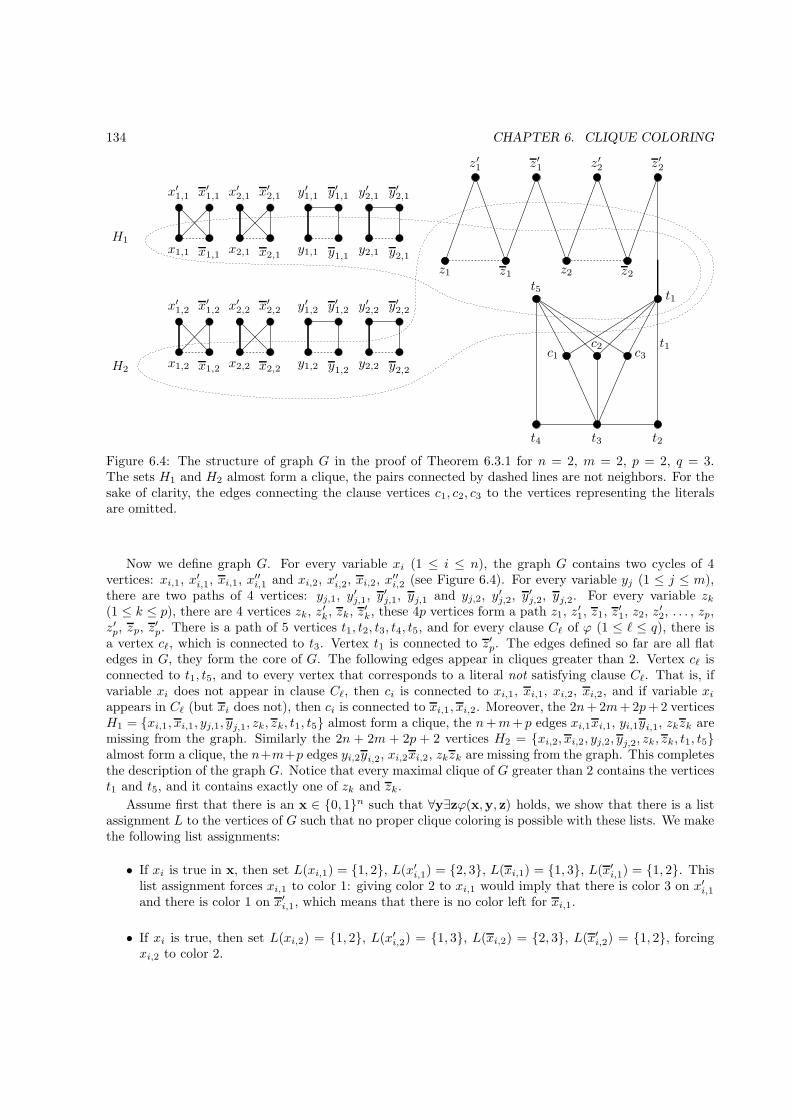
134 CHAPTER 6. CLIQUE COLORING
z1
y′2,2
y2,2y2,2
y′2,2y′1,2
y1,2 y1,2
y′1,2
x2,2
x′2,2x′2,2
x2,2x1,2
x′1,2 x′1,2
x1,2
y′2,1
y2,1 y2,1
y′2,1y′1,1
y1,1y1,1
y′1,1
x2,1
x′2,1 x′2,1
x2,1x1,1
x′1,1x′1,1
x1,1
c1c2
c3
t4 t2t3
t1
t1t5
H2
H1
z′2z′2z′1z′1
z1 z2z2
Figure 6.4: The structure of graph G in the proof of Theorem 6.3.1 for n = 2, m = 2, p = 2, q = 3.The sets H1 and H2 almost form a clique, the pairs connected by dashed lines are not neighbors. For thesake of clarity, the edges connecting the clause vertices c1, c2, c3 to the vertices representing the literalsare omitted.
Now we define graph G. For every variable xi (1 ≤ i ≤ n), the graph G contains two cycles of 4vertices: xi,1, x′i,1, xi,1, x′′i,1 and xi,2, x′i,2, xi,2, x′′i,2 (see Figure 6.4). For every variable yj (1 ≤ j ≤ m),there are two paths of 4 vertices: yj,1, y′j,1, y′j,1, yj,1 and yj,2, y′j,2, y′j,2, yj,2. For every variable zk(1 ≤ k ≤ p), there are 4 vertices zk, z′k, zk, z′k, these 4p vertices form a path z1, z′1, z1, z′1, z2, z′2, . . . , zp,z′p, zp, z
′p. There is a path of 5 vertices t1, t2, t3, t4, t5, and for every clause Cℓ of ϕ (1 ≤ ℓ ≤ q), there is
a vertex cℓ, which is connected to t3. Vertex t1 is connected to z′p. The edges defined so far are all flatedges in G, they form the core of G. The following edges appear in cliques greater than 2. Vertex cℓ isconnected to t1, t5, and to every vertex that corresponds to a literal not satisfying clause Cℓ. That is, ifvariable xi does not appear in clause Cℓ, then ci is connected to xi,1, xi,1, xi,2, xi,2, and if variable xiappears in Cℓ (but xi does not), then ci is connected to xi,1, xi,2. Moreover, the 2n+ 2m+ 2p+ 2 verticesH1 = {xi,1, xi,1, yj,1, yj,1, zk, zk, t1, t5} almost form a clique, the n+m+ p edges xi,1xi,1, yi,1yi,1, zkzk aremissing from the graph. Similarly the 2n + 2m + 2p + 2 vertices H2 = {xi,2, xi,2, yj,2, yj,2, zk, zk, t1, t5}almost form a clique, the n+m+p edges yi,2yi,2, xi,2xi,2, zkzk are missing from the graph. This completesthe description of the graph G. Notice that every maximal clique of G greater than 2 contains the verticest1 and t5, and it contains exactly one of zk and zk.
Assume first that there is an x ∈ {0, 1}n such that ∀y∃zϕ(x,y, z) holds, we show that there is a listassignment L to the vertices of G such that no proper clique coloring is possible with these lists. We makethe following list assignments:
• If xi is true in x, then set L(xi,1) = {1, 2}, L(x′i,1) = {2, 3}, L(xi,1) = {1, 3}, L(x′i,1) = {1, 2}. Thislist assignment forces xi,1 to color 1: giving color 2 to xi,1 would imply that there is color 3 on x′i,1and there is color 1 on x′i,1, which means that there is no color left for xi,1.
• If xi is true, then set L(xi,2) = {1, 2}, L(x′i,2) = {1, 3}, L(xi,2) = {2, 3}, L(x′i,2) = {1, 2}, forcingxi,2 to color 2.
6.3. CLIQUE CHOOSABILITY 135
• If xi is false, then set L(xi,1) = {1, 3}, L(x′i,1) = {2, 3}, L(xi,1) = {1, 2}, L(x′i,1) = {1, 2}, forcingxi,1 to color 1.
• If xi is false, then set L(xi,2) = {2, 3}, L(x′i,2) = {1, 3} L(xi,2) = {1, 2}, L(x′i,2) = {1, 2}, forcing xi,2to color 2.
Set L(v) = {1, 2} for every other vertex v. We claim that there is no proper clique coloring with these listassignments.
Assume that, on the contrary, there is a proper clique coloring ψ. Since the edges titi+1 (1 ≤ i ≤ 4)are flat edges, the vertices t1, t3, t5 have the same color, suppose first that it is color 1. Then every vertexcℓ has color 2 (edge t3cℓ is a flat edge) and the vertices zk, zk (1 ≤ k ≤ p have color 1 (every edge of thepath from z1 to t1 is a flat edge and the vertices in the path have the list {1, 2}). For every 1 ≤ j ≤ m,exactly one of yj,1 and yj,1 have color 1, since edges yj,1y
′j,1, y
′j,1y
′j,1, y
′j,1yj,1 are flat edges. Define the
vector y ∈ {0, 1}m such that variable yj is true if and only if yj,1 has color 1. By assumption, there is avector z such that ϕ(x,y, z) holds. Based on x, y, and z, we can define a clique K of G as follows:
• xi,1 ∈ K iff xi is true,
• xi,1 ∈ K iff xi is false,
• yj,1 ∈ K iff yj is true,
• yj,1 ∈ K iff yj is false,
• zk ∈ K iff zk is true,
• zk ∈ K iff zk is false,
• t1, t5 ∈ K.
Notice that every vertex in clique K has color 1: if xi is true (resp. false) then the list assignments forcexi,1 (resp. xi,1) to color 1. Moreover, exactly one of yj,1 and yj,1 have color 1, and the definition of y andK implies that from these two vertices, the one with color 1 is selected into K. By assumption, ψ is aproper clique coloring, therefore K is not a maximal clique. It is clear that only a vertex cℓ can extendK to a larger clique, thus there is a cℓ such that K ∪ {cℓ} is also a clique. However, by the construction,this means that in ϕ(x,y, z), no variable satisfies clause Cℓ, a contradiction.
If vertices t1, t3, t5 have color 2, then we proceed similarly. Vector y is defined such that yj is true ifand only if yi,2 has color 2. In this case the definition of K is similar, but now K contains the verticesxi,2, xi,2, yj,2, yj,2 instead of xi,1, xi,1, yj,1, yj,1. Every vertex in K has color 2: the list assignment ensuresthat if variable xi is true, then vertex xi,2 has color 2. The other parts of the proof remain the same.
To prove the other direction, we show that if ∃x∀y∃zϕ(x,y, z) does not hold, then there is properclique coloring for every list assignment L. The core of G is the disjoint union of trees and even cycles,hence it is 2-choosable. In particular, the path T = t1, t2, . . . , t5 can be colored with the lists, and everycoloring of T can be extended to an L-coloring of the core of G. If there is a coloring of this path suchthat t1 and t5 have different color, then this can be extended to a proper vertex coloring of the core of G.Moreover, this coloring is also a proper clique coloring of G: every maximal clique greater than 2 containsboth t1 and t5, thus the clique contains at least two different colors. Therefore, if the list assignment isuncolorable, then it can be assumed that in every coloring of the path T , vertices t1 and t5 receive thesame color. It is easy to verify that this is only possible if all 5 vertices of T have the same list, say {1, 2}.In this case we give color 1 to the vertices t1, t3, t5, and color 2 to vertices t2, t4. Color the path from z1to z′p with arbitrary colors. Furthermore, give a color different from 1 to every vertex cℓ.
The rest of the graph is colored as follows. The length 4 cycle formed by the vertices xi,1, x′i,1, xi,1, x
′′i,1
is 2-choosable, thus it can be colored with the given lists. Moreover, it can be verified by a simple case
136 CHAPTER 6. CLIQUE COLORING
analysis that we can choose a coloring that does not assign color 1 to both xi,1 and xi,1. The verticesxi,2, x
′i,2, xi,2, x
′′i,2 are colored similarly. Define the vectors x1,x2 ∈ {0, 1}n such that variable x1
i (resp. x2i )
is true if and only if vertex xi,1 (resp, xi,2) has color 1.By assumption, ∃x∀y∃zϕ(x,y, z) does not hold, thus ∀y∃zϕ(x1 ,y, z) and ∀y∃zϕ(x2 ,y, z) are false
in particular. Therefore there are vectors y1,y2 ∈ {0, 1}m such that ∃zϕ(x1,y1, z) does not hold and∃zϕ(x2,y2, z) does not hold. Based on the vectors y1, y2, we continue the coloring of G. The path yi,1,y′i,1, y′i,1, yi,1 can be colored with the lists. Moreover, this path has a coloring such that yi,1 does not have
color 1, and it has another coloring where yi,1 does not have color 1. If y1i is true (resp. false), then color
the path in such a way that yi,1 (resp. yi,1) has a color different from 1. Color the path yi,2, y′i,2, y′i,2, yi,2analogously. We claim that this coloring is a proper clique coloring. Since the coloring is a proper vertexcoloring of the core of G, it is sufficient to check the maximal cliques greater than 2. Since every suchclique K contains the vertices t1 and t5 having color 1, thus every vertex in K has color 1. This impliesthat K does not contain any of the vertices cℓ, since we have assigned colors different from 1 to thesevertices. For every 1 ≤ k ≤ p, clique K contains exactly one of zk and zk. Define the vector z ∈ {0, 1}p
such that variable zk is true if and only if zk ∈ K. Clique K contains exactly one of xi,1, xi,1, xi,2,xi,2, suppose that it contains xi,1 or xi,1 (the other case is handled analogously). Since K contains onlyvertices with color 1, and at most one of xi,1 and xi,1 has color 1, thus xi,1 ∈ K if and only if x1
i is true.Similarly, K contains exactly one of yi,1 and yi,1, more precisely, yi,1 ∈ K if and only if y1
i is true. Toarrive to a contradiction, we show that ϕ(x1,y1, z) is true. Suppose that clause Cℓ is not satisfied by thisvariable assignment. The vertices in K correspond to the true literals in the variable assignment x1,y1, z,therefore by the construction, cℓ is connected to every vertex in K, contradicting the assumption that Kis a maximal clique. �
The k-Clique-Choosability problem remains Πp3-complete for every k > 2. The proof is similar to the
proof of Corollary 6.2.2: the case k is reduced to the case k+1 by attaching some special graphs. However,here we attach complete bipartite graphs instead of Mycielski graphs.
Lemma 6.3.2. There is k-vertex-choosable bipartite graph Bk with a distinguished vertex x that has thefollowing property: for every color c there is a k-list assignment such that in every list coloring x receivescolor c.
Proof. We claim that the complete bipartite graph Bk = Kk,kk−1 is such a graph, with x ∈ V1 being avertex of the smaller class V1. To see that Bk is k-vertex-choosable, assume first that L(u) ∩ L(v) 6= ∅for some u, v ∈ V1. In this case the k vertices in V1 can be colored such that they receive at most k − 1distinct colors, thus every vertex w ∈ V2 can be given a color from L(w) that is not used by the vertices inV1. If the lists in V1 are disjoint, then V1 can be colored in kk different ways, every such coloring assignsa different set of k colors to the vertices in V1. A coloring of V1 can be extended to V2 unless there is avertex w ∈ V2 whose list contains exactly the k colors used by V1. Since there are only kk − 1 vertices inV2, they can exclude at most kk − 1 colorings of V1, thus at least one of the kk different colorings of V1
can be extended to V2.On the other hand, let V1 = {v1, . . . , vk} and L(vi) = {ci,1, ci,2, . . . , ci,k}. There are kk sets of
the form {c1,i1 , c2,i2 , . . . , ck,ik} with 1 ≤ i1, i2, . . . , ik ≤ k. Assign these sets, with the exception of{c1,1, c2,1, . . . , ck,1}, to the vertices in V2. It is easy to see that with these list assignments, every coloringgives color ci,1 to vertex vi. Therefore x = v1 and c = c1,1 satisfies the requirements. �
Corollary 6.3.3. For every k ≥ 2, k-Clique-Choosability is Πp3-complete.
Proof. For every k ≥ 2, we give a polynomial time reduction from k-Clique-Choosability to (k + 1)-Clique-Choosability. By Theorem 6.3.1, 2-Clique-Choosability is Πp
3-complete, thus the theorem followsby induction.
Let G(V,E) be a graph with n vertices v1, v2, . . . , vn. Add n disjoint copies of the graph Bk+1
(Lemma 6.3.2) such that vertex xi, which is the distinguished vertex x of the ith copy, is connected
6.4. HEREDITARY CLIQUE COLORING 137
to vi. Denote by W the new vertices added to G, observe that every vertex in W is simple (Bk+1 isbipartite, thus it does not contain triangles). We claim that the resulting graph G′(V ∪W,E′) is (k + 1)-clique-choosable if and only if G is k-clique-choosable.
Assume first that G′ is (k + 1)-clique-choosable, we show that G is k-clique-choosable. Let L be anarbitrary k-assignment of G. Let c be a color not appearing in L. Define the (k + 1)-assignment L′ asL′(v) = L(v)∪{c} for every v ∈ V , and extend L′ to W (i.e., to the copies of Bk+1) in such a way that inevery list coloring of G′, the vertices xi receive the color c. By assumption, G′ has a clique coloring ψ withthe lists L′. By Prop. 6.1.3, ψ is a proper vertex coloring of W , therefore ψ(xi) = c for every 1 ≤ i ≤ n.Thus ψ(vi) 6= c and ψ(vi) ∈ L(vi) follow, hence ψ induces a list coloring of G. Moreover, by Prop. 6.1.1,ψ is a proper clique coloring of G, proving this direction of the reduction.
Now assume that G is k-clique-choosable, it has to be shown that G′ is (k + 1)-clique-choosable. LetL be a k + 1 assignment of V ∪W . Since Bk+1 is (k + 1)-choosable, every copy of Bk+1 can be coloredwith these lists, let ψ be this coloring of W . Define the k-assignment L′ of V as L′(vi) = L(vi) \ {ψ(xi)}if ψ(xi) ∈ L(vi), otherwise let L′(vi) an arbitrary k element subset of L(vi). By assumption, there is aproper clique coloring of V with the lists L′, extend ψ to V with these assignment of colors. By Prop. 6.1.2,ψ is also a proper clique coloring of G′. �
6.4 Hereditary clique coloring
Graph G is hereditary k-clique-colorable if every induced subgraph of G is k-clique-colorable. Since cliquecoloring is not a hereditary property in general, an induced subgraph of a k-clique-colorable graph G is notnecessarily k-clique-colorable, thus hereditary k-clique-colorability is not the same as k-clique-colorability.The main result of this section is that we show that Hereditary k-Clique-Coloring is Πp
3-complete for everyk ≥ 3.
Hereditary k-Clique-Coloring
Input: A graph G(V,E)
Question: Is it true that every induced subgraph of G is k-clique-colorable?
The proof follows the same general framework as the proof of Theorem 6.3.1, but selecting an inducedsubgraph of G plays here the same role as selecting a list assignment in that proof. To show that∃x∀y∃zϕ(x,y, z) implies that G is not hereditary 3-clique-colorable, assume that a vector x exists with∀y∃zϕ(x,y, z). Based on this vector x, we select an induced subgraph G(x) of G. If subgraph G(x) hasa 3-clique-coloring ψ, then a vector y can be defined based on ψ. By assumption, there is a vector z suchthat ϕ(x,y, z) is true. We arrive to a contradiction by showing that vectors x,y, z can be used to find amonochromatic maximal clique K in ψ. The overview of this direction:
A vectorx with
∀y∃zϕ(x,y, z)⇒
A subgraphG(x) of G
⇒An arbitrary
coloringψ of G(x)
⇒ A vector y ⇒A vectorz with
ϕ(x,y, z) = 1⇒
A monochro-matic cliqueK in ψ
The proof of the reverse direction is much more delicate. We have to show that if there is an inducedsubgraph G′ of G that is not 3-clique-colorable, then ∃x∀y∃zϕ(x,y, z) holds. If G′ is a subgraph G(x)for some vector x (as defined by the first direction of the proof), then we proceed as follows. Assume that∃x∀y∃zϕ(x,y, z) does not hold, then there is vector y with ∄zϕ(x,y, z). Based on this vector y, one candefine a 3-coloring ψ of G′. By assumption, G′ is not 3-clique-colorable, thus ψ contains a monochromaticmaximal clique K. Now we can a find a vector z satisfying ϕ(x,y, z), a contradiction.
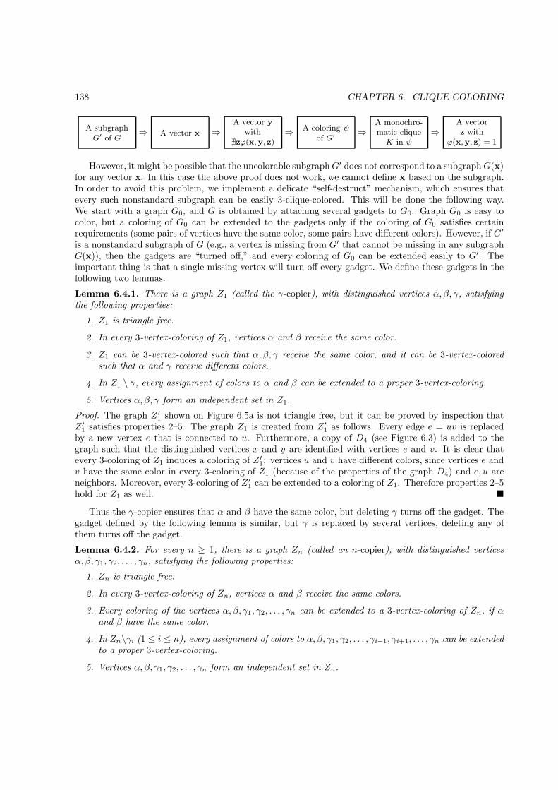
138 CHAPTER 6. CLIQUE COLORING
A subgraphG′ of G
⇒ A vector x ⇒A vector y
with∄zϕ(x,y, z)
⇒ A coloring ψof G′
⇒A monochro-matic cliqueK in ψ
⇒A vectorz with
ϕ(x,y, z) = 1
However, it might be possible that the uncolorable subgraphG′ does not correspond to a subgraphG(x)for any vector x. In this case the above proof does not work, we cannot define x based on the subgraph.In order to avoid this problem, we implement a delicate “self-destruct” mechanism, which ensures thatevery such nonstandard subgraph can be easily 3-clique-colored. This will be done the following way.We start with a graph G0, and G is obtained by attaching several gadgets to G0. Graph G0 is easy tocolor, but a coloring of G0 can be extended to the gadgets only if the coloring of G0 satisfies certainrequirements (some pairs of vertices have the same color, some pairs have different colors). However, if G′
is a nonstandard subgraph of G (e.g., a vertex is missing from G′ that cannot be missing in any subgraphG(x)), then the gadgets are “turned off,” and every coloring of G0 can be extended easily to G′. Theimportant thing is that a single missing vertex will turn off every gadget. We define these gadgets in thefollowing two lemmas.
Lemma 6.4.1. There is a graph Z1 (called the γ-copier), with distinguished vertices α, β, γ, satisfyingthe following properties:
1. Z1 is triangle free.
2. In every 3-vertex-coloring of Z1, vertices α and β receive the same color.
3. Z1 can be 3-vertex-colored such that α, β, γ receive the same color, and it can be 3-vertex-coloredsuch that α and γ receive different colors.
4. In Z1 \ γ, every assignment of colors to α and β can be extended to a proper 3-vertex-coloring.
5. Vertices α, β, γ form an independent set in Z1.
Proof. The graph Z ′1 shown on Figure 6.5a is not triangle free, but it can be proved by inspection that
Z ′1 satisfies properties 2–5. The graph Z1 is created from Z ′
1 as follows. Every edge e = uv is replacedby a new vertex e that is connected to u. Furthermore, a copy of D4 (see Figure 6.3) is added to thegraph such that the distinguished vertices x and y are identified with vertices e and v. It is clear thatevery 3-coloring of Z1 induces a coloring of Z ′
1: vertices u and v have different colors, since vertices e andv have the same color in every 3-coloring of Z1 (because of the properties of the graph D4) and e, u areneighbors. Moreover, every 3-coloring of Z ′
1 can be extended to a coloring of Z1. Therefore properties 2–5hold for Z1 as well. �
Thus the γ-copier ensures that α and β have the same color, but deleting γ turns off the gadget. Thegadget defined by the following lemma is similar, but γ is replaced by several vertices, deleting any ofthem turns off the gadget.
Lemma 6.4.2. For every n ≥ 1, there is a graph Zn (called an n-copier), with distinguished verticesα, β, γ1, γ2, . . . , γn, satisfying the following properties:
1. Zn is triangle free.
2. In every 3-vertex-coloring of Zn, vertices α and β receive the same colors.
3. Every coloring of the vertices α, β, γ1, γ2, . . . , γn can be extended to a 3-vertex-coloring of Zn, if αand β have the same color.
4. In Zn\γi (1 ≤ i ≤ n), every assignment of colors to α, β, γ1, γ2, . . . , γi−1, γi+1, . . . , γn can be extendedto a proper 3-vertex-coloring.
5. Vertices α, β, γ1, γ2, . . . , γn form an independent set in Zn.
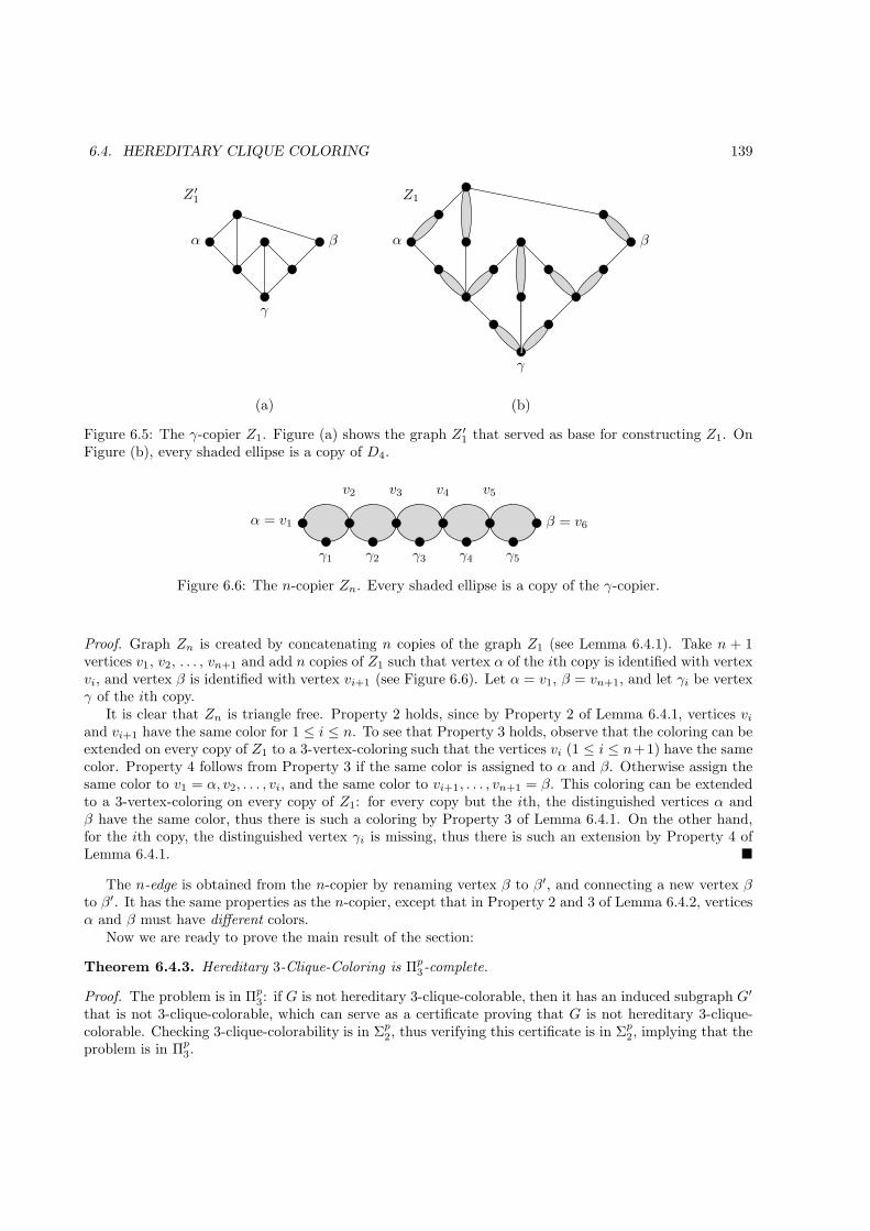
6.4. HEREDITARY CLIQUE COLORING 139
Z1Z ′1
(a) (b)
γ
γ
β βα α
Figure 6.5: The γ-copier Z1. Figure (a) shows the graph Z ′1 that served as base for constructing Z1. On
Figure (b), every shaded ellipse is a copy of D4.
γ1 γ2 γ3 γ4 γ5
α = v1
v2 v3 v4 v5
β = v6
Figure 6.6: The n-copier Zn. Every shaded ellipse is a copy of the γ-copier.
Proof. Graph Zn is created by concatenating n copies of the graph Z1 (see Lemma 6.4.1). Take n + 1vertices v1, v2, . . . , vn+1 and add n copies of Z1 such that vertex α of the ith copy is identified with vertexvi, and vertex β is identified with vertex vi+1 (see Figure 6.6). Let α = v1, β = vn+1, and let γi be vertexγ of the ith copy.
It is clear that Zn is triangle free. Property 2 holds, since by Property 2 of Lemma 6.4.1, vertices viand vi+1 have the same color for 1 ≤ i ≤ n. To see that Property 3 holds, observe that the coloring can beextended on every copy of Z1 to a 3-vertex-coloring such that the vertices vi (1 ≤ i ≤ n+1) have the samecolor. Property 4 follows from Property 3 if the same color is assigned to α and β. Otherwise assign thesame color to v1 = α, v2, . . . , vi, and the same color to vi+1, . . . , vn+1 = β. This coloring can be extendedto a 3-vertex-coloring on every copy of Z1: for every copy but the ith, the distinguished vertices α andβ have the same color, thus there is such a coloring by Property 3 of Lemma 6.4.1. On the other hand,for the ith copy, the distinguished vertex γi is missing, thus there is such an extension by Property 4 ofLemma 6.4.1. �
The n-edge is obtained from the n-copier by renaming vertex β to β′, and connecting a new vertex βto β′. It has the same properties as the n-copier, except that in Property 2 and 3 of Lemma 6.4.2, verticesα and β must have different colors.
Now we are ready to prove the main result of the section:
Theorem 6.4.3. Hereditary 3-Clique-Coloring is Πp3-complete.
Proof. The problem is in Πp3: if G is not hereditary 3-clique-colorable, then it has an induced subgraph G′
that is not 3-clique-colorable, which can serve as a certificate proving that G is not hereditary 3-clique-colorable. Checking 3-clique-colorability is in Σp2, thus verifying this certificate is in Σp2, implying that theproblem is in Πp
3.
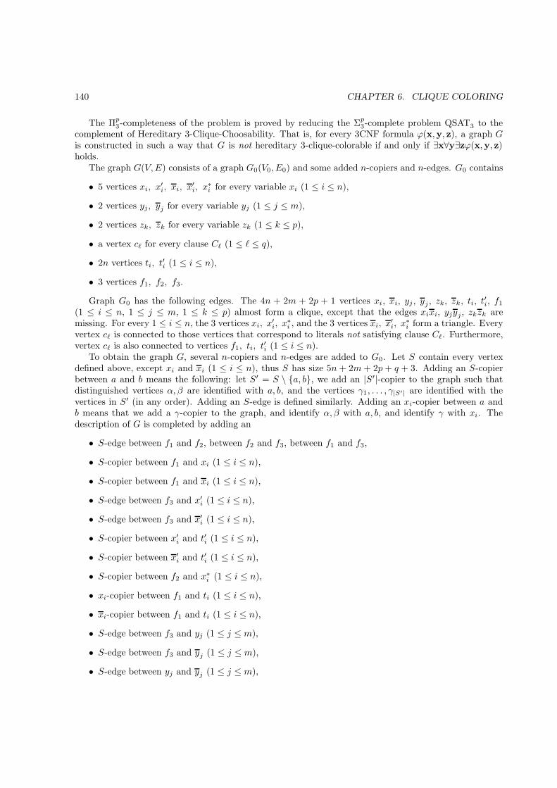
140 CHAPTER 6. CLIQUE COLORING
The Πp3-completeness of the problem is proved by reducing the Σp3-complete problem QSAT3 to the
complement of Hereditary 3-Clique-Choosability. That is, for every 3CNF formula ϕ(x,y, z), a graph Gis constructed in such a way that G is not hereditary 3-clique-colorable if and only if ∃x∀y∃zϕ(x,y, z)holds.
The graph G(V,E) consists of a graph G0(V0, E0) and some added n-copiers and n-edges. G0 contains
• 5 vertices xi, x′i, xi, x
′i, x
∗i for every variable xi (1 ≤ i ≤ n),
• 2 vertices yj, yj for every variable yj (1 ≤ j ≤ m),
• 2 vertices zk, zk for every variable zk (1 ≤ k ≤ p),
• a vertex cℓ for every clause Cℓ (1 ≤ ℓ ≤ q),
• 2n vertices ti, t′i (1 ≤ i ≤ n),
• 3 vertices f1, f2, f3.
Graph G0 has the following edges. The 4n + 2m + 2p + 1 vertices xi, xi, yj , yj , zk, zk, ti, t′i, f1
(1 ≤ i ≤ n, 1 ≤ j ≤ m, 1 ≤ k ≤ p) almost form a clique, except that the edges xixi, yjyj , zkzk aremissing. For every 1 ≤ i ≤ n, the 3 vertices xi, x
′i, x
∗i , and the 3 vertices xi, x
′i, x
∗i form a triangle. Every
vertex cℓ is connected to those vertices that correspond to literals not satisfying clause Cℓ. Furthermore,vertex cℓ is also connected to vertices f1, ti, t
′i (1 ≤ i ≤ n).
To obtain the graph G, several n-copiers and n-edges are added to G0. Let S contain every vertexdefined above, except xi and xi (1 ≤ i ≤ n), thus S has size 5n+ 2m+ 2p+ q + 3. Adding an S-copierbetween a and b means the following: let S′ = S \ {a, b}, we add an |S′|-copier to the graph such thatdistinguished vertices α, β are identified with a, b, and the vertices γ1, . . . , γ|S′| are identified with thevertices in S′ (in any order). Adding an S-edge is defined similarly. Adding an xi-copier between a andb means that we add a γ-copier to the graph, and identify α, β with a, b, and identify γ with xi. Thedescription of G is completed by adding an
• S-edge between f1 and f2, between f2 and f3, between f1 and f3,
• S-copier between f1 and xi (1 ≤ i ≤ n),
• S-copier between f1 and xi (1 ≤ i ≤ n),
• S-edge between f3 and x′i (1 ≤ i ≤ n),
• S-edge between f3 and x′i (1 ≤ i ≤ n),
• S-copier between x′i and t′i (1 ≤ i ≤ n),
• S-copier between x′i and t′i (1 ≤ i ≤ n),
• S-copier between f2 and x∗i (1 ≤ i ≤ n),
• xi-copier between f1 and ti (1 ≤ i ≤ n),
• xi-copier between f1 and ti (1 ≤ i ≤ n),
• S-edge between f3 and yj (1 ≤ j ≤ m),
• S-edge between f3 and yj (1 ≤ j ≤ m),
• S-edge between yj and yj (1 ≤ j ≤ m),
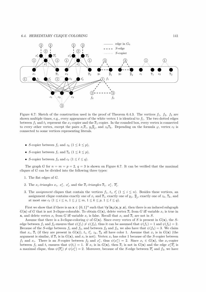
6.4. HEREDITARY CLIQUE COLORING 141
t2
z1
f3
z1
f1
y2y1 y2
t1
x1 y1x1
c3
x2 z2x2
c1 c2
t′2
f2
t′1
z2
x∗
1 x∗
2
x′
1 x′
2x′
1 x′
2
edge in G0
S-edge
S-copier
1 11111
1 1 1
3
333 3
33
3
2
22
Figure 6.7: Sketch of the construction used in the proof of Theorem 6.4.3. The vertices f1, f2, f3 areshown multiple times, e.g., every appearance of the white vertex 1 is identical to f1. The two dotted edgesbetween f1 and t1 represent the x1-copier and the x1-copier. In the rounded box, every vertex is connectedto every other vertex, except the pairs xixi, yjyj , and zkzk. Depending on the formula ϕ, vertex cℓ isconnected to some vertices representing literals.
• S-copier between f1 and zk (1 ≤ k ≤ p),
• S-copier between f1 and zk (1 ≤ k ≤ p),
• S-copier between f3 and cℓ (1 ≤ ℓ ≤ q).
The graph G for n = m = p = 2, q = 3 is shown on Figure 6.7. It can be verified that the maximalcliques of G can be divided into the following three types:
1. The flat edges of G.
2. The xi-triangles xi, x∗i , x
′i, and the xi-triangles xi, x
∗i , x
′i.
3. The assignment cliques that contain the vertices f1, ti, t′i (1 ≤ i ≤ n). Besides these vertices, an
assignment clique contains exactly one of xi and xi, exactly one of yj , yj , exactly one of zk, zk, andat most one cℓ (1 ≤ i ≤ n, 1 ≤ j ≤ m, 1 ≤ k ≤ p, 1 ≤ ℓ ≤ q).
First we show that if there is an x ∈ {0, 1}n such that ∀y∃zϕ(x,y, z), then there is an induced subgraphG(x) of G that is not 3-clique-colorable. To obtain G(x), delete vertex xi from G iff variable xi is true inx, and delete vertex xi from G iff variable xi is false. Recall that xi and xi are not in S.
Assume that there is a 3-clique-coloring ψ of G(x). Since every vertex of S is present in G(x), the S-edge between f1 and f2 ensures that ψ(f1) 6= ψ(f2), thus it can be assumed that ψ(f1) = 1 and ψ(f2) = 2.Because of the S-edge between f1 and f3, and between f2 and f3, we also have that ψ(f3) = 3. We claimthat xi, xi (if they are present in G(x)), ti, t
′i, zk, zk all have color 1. Assume that xi is in G(x) (the
argument is similar, if xi is in G(x), and xi is not). Vertex xi has color 1 because of the S-copier betweenf1 and xi. There is an S-copier between f2 and x∗i , thus ψ(x∗i ) = 2. Since xi ∈ G(x), the xi-copierbetween f1 and ti ensures that ψ(ti) = 1. If xi is in G(x), then xi is not in G(x) and the edge x∗i x
′i is
a maximal clique, thus ψ(x′i) 6= ψ(x∗i ) = 2. Moreover, because of the S-edge between x′i and f3, we have
142 CHAPTER 6. CLIQUE COLORING
ψ(x′i) 6= 3, implying ψ(x′i) = 1. Since there is an S-copier between x′i and t′i, hence ψ(t′i) = 1. Finally, theS-copier between f1 and zk, and between f1 and zk implies that ψ(zk) = ψ(zk) = 1.
The S-edge between f3 and yj , and between f3 and yj ensure that yj and yj have color 1 or 2.Furthermore, because of the S-edge between yj and yj , one of them has color 1, and the other has color 2.Define the vector y ∈ {0, 1}m such that variable yj is true if and only if ψ(yj) = 1. By assumption, thereis a vector z ∈ {0, 1}p such that ϕ(x,y, z) is true. Let K contain all the vertices of G(x) that correspondsto true literals in x,y, z. Moreover, add to K the vertices f1, ti, t
′i (1 ≤ i ≤ n). Clearly, K is a clique.
Furthermore, because of the way K was constructed, every vertex in K has color 1. We claim that K is amonochromatic maximal clique, contradicting the assumption that ψ is a proper 3-clique-coloring of G(x).It is easy to see that only a vertex cℓ corresponding to a clause might extend K to larger clique. However,in this case the assignment x, y, z does not satisfy ϕ since clause Cℓ is not satisfied: otherwise there isa vertex in K that corresponds to a literal satisfying Cℓ, and by the construction cℓ is not connected tothis vertex.
To prove the other direction of the reduction, assume that there is an induced subgraph G′ of Gthat is not 3-clique-colorable, we have to show that ∃x∀y∃zϕ(x,y, z) holds. By Prop. 6.1.1, it can beassumed that G′ contains all the simple vertices of G: adding simple vertices to G′ does not make it3-clique-colorable.
Call an induced subgraph of G standard, if for every 1 ≤ i ≤ n, it contains exactly one of xi and xi,and it contains every other vertex of G (in particular, it contains every vertex of S). First we show thatevery nonstandard subgraph of G is 3-clique-colorable, thus G′ must be standard. Next we show that ifthere is a standard subgraph G′ of G that is not 3-clique-colorable, then there is an x ∈ {0, 1}n satisfying∀y∃zϕ(x,y, z). These two lemmas complete the proof of this direction of the reduction.
Lemma 6.4.4. If G′ is a nonstandard induced subgraph of G, then G′ is 3-clique-colorable.
Proof. Let G′ be a nonstandard subgraph of G. By Lemma 6.1.1 it can be assumed that G′ containsevery simple vertex of G. Moreover, we show that G′ contains every vertex of S. Assume that a vertexv ∈ S is missing from G′. The absence of v turns off the S-copiers and the S-edges, which makes thecoloring very easy. However, the xi-copiers might still be working. Let G′
0 be the induced subgraph of G′
containing only those vertices that are in G0. We show that there is a 3-clique-coloring of G′0 with the
following property: if both f1 and ti are in G′0 for some 1 ≤ i ≤ n, and at least one of xi, xi is in G′
0, thenf1 and ti have the same color. If this is true, then this coloring can be extended to a 3-clique-coloring ofG′: by Property 4 of Lemma 6.4.2, the coloring can be extended to every S-copier and S-edge, since v ∈ Sis missing from G′. Here we use Prop. 6.1.2: if we extend the coloring of G′
0 such that every gadget is3-vertex-colored, then it gives a 3-clique-coloring of G. Moreover, the xi-copier and the xi-copier betweenf1 and ti can be colored as well, since both xi and xi are missing (Property 4 of Lemma 6.4.1), or f1 andti have the same color (Property 3 of Lemma 6.4.1).
To see that such a coloring of G′0 exists, consider the following assignment of colors:
• Vertices f1, x′i, x
′i, ti, t
′i have color 1 (1 ≤ i ≤ n).
• Vertices f2, xi, xi, yj , yj , zk, zk have color 2 (1 ≤ i ≤ n, 1 ≤ j ≤ m, 1 ≤ k ≤ p).
• Vertices f3, x∗i , cℓ have color 3 (1 ≤ i ≤ n, 1 ≤ ℓ ≤ q).
This is a proper 3-clique-coloring of G′0 if at least one of T1 = {f1, x′i, x
′i, ti, t
′i} and at least one of
T2 = {f2, xi, xi, yj , yj , zk, zk} is present in G′0, it can be verified that a clique with color 1 can be extended
by a vertex with color 2, and a clique with color 2 can be extended by a vertex with color 1. The twospecial cases, when either all of T1 or all of T2 is missing, have to be considered separately. However, thesecases are easy to handle, the details are left to the reader.
Now assume that G′ is a nonstandard subgraph of G and every vertex of S is in G′. Since the graph isnonstandard, there is an 1 ≤ i0 ≤ n such that either G′ contains both xi0 and xi0 , or G′ contains neitherxi0 nor xi0 . The following coloring of G′
0 can be extended to a proper 3-clique-coloring of G′:
6.4. HEREDITARY CLIQUE COLORING 143
• Vertices f1, xi, xi, x′i, x
′i, ti, t
′i have color 1, where 1 ≤ i ≤ n and i 6= i0.
• Vertices yj , yj , zk, zk have color 1 (1 ≤ j ≤ m, 1 ≤ k ≤ p)
• Vertices f2, x∗i have color 2 (1 ≤ i ≤ n).
• Vertices f3, cℓ have color 3 (1 ≤ ℓ ≤ q).
• If both xi0 and xi0 are in G′, then x′i0 , x′i0 , t′i0 have color 2 and xi0 , xi0 , ti0 have color 1.
• If neither xi0 nor xi0 are in G′, then x′i0 , x′i0 , t′i0 have color 1 and ti0 has color 2.
This coloring can be extended to G′ in such a way that the flat edges are properly colored (that is, it can beextended to the internal vertices of the copier and edge gadgets). Indeed, it can be verified by inspectionthat the two distinguished vertices of the S-copiers (resp. S-edges) have the same (resp. different) colors,respectively. Moreover, for i 6= i0, both f1 and ti have color 1, thus the coloring can be extended to thexi-copier and xi-copier between f1 and ti. However, if both xi0 and xi0 are missing from G′, then f1has color 1 and ti0 has color 2. But in this case the absence of xi0 and xi0 ensures that the two copiersbetween f1 and ti0 can be colored, regardless of the color of f1 and ti0 (Property 4 of Lemma 6.4.1).
The triangles xi, x∗i , x
′i and xi, x
∗i , x
′i contain both color 1 and 2. Therefore only the assignment
cliques can be monochromatic in this coloring. However, every assignment clique contains ti0 and t′i0 , andthese two vertices have different colors. �
Therefore we can assume that G′ is a standard subgraph. We show that based on G′ we can define anassignment x such that ∀y∃zϕ(x,y, z). The proof is similar to the proof of the first direction.
Lemma 6.4.5. If there is a standard subgraph G′ of G that is not 3-clique-colorable, then there is anx ∈ {0, 1}n satisfying ∀y∃zϕ(x,y, z).
Proof. Define vector x ∈ {0, 1}n by setting variable xi to true if xi ∈ G′, and to false if xi ∈ G′. We claimthat ∀y∃zϕ(x,y, z). Suppose that, on the contrary, there is a vector y ∈ {0, 1}m such that ϕ(x,y, z) isfalse for every z ∈ {0, 1}p.
Consider the following coloring of G′:
• Vertices f1, xi, xi, x′i, x
′i, t
′i, ti, zk, zk have color 1 (1 ≤ i ≤ n, 1 ≤ k ≤ p).
• Vertices f2, x∗i have color 2 (1 ≤ i ≤ n).
• Vertices f3, cℓ have color 3 (1 ≤ ℓ ≤ q).
• If variable yj is true in y, then vertex yj has color 1 and vertex yj has color 2 (1 ≤ j ≤ m).
• If variable yj is false in y, then vertex yj has color 2 and vertex yj has color 1 (1 ≤ j ≤ m).
As in the proof of the previous lemma, this coloring can be extended to the whole G′ in such a way thatevery flat edge and every xi-triangle is properly colored. By assumption, this coloring is not a proper3-clique-coloring, thus there is a monochromatic maximal clique K, which must be an assignment clique.Since every assignment clique contains f1, therefore every vertex of K has color 1. By the definition of thecoloring, this means that K contains yj if and only if yj is true in y. For every 1 ≤ k ≤ p, an assignmentclique contains exactly one of zk and zk, define the vector z ∈ {0, 1}p by setting variable zk to true if andonly if zk ∈ K. Notice that apart from f1, ti, t
′i, clique K contains those vertices that correspond to true
literals in the assignment x,y, z.We claim that ϕ(x,y, z) is true. To see this, assume that clause Cℓ is not satisfied by this assignment.
Vertex cℓ is not in K, since cℓ has color 3. Now clique K contains the vertices f1, ti, t′i, and vertices
corresponding literals not satisfying Cℓ, therefore K ∪ {cℓ} is also a clique, contradicting the maximalityof K. �
Putting together these two lemmas completes the proof of the theorem. �
144 CHAPTER 6. CLIQUE COLORING
Hereditary k-clique-coloring is also Πp3-complete for every k > 3. The proof is analogous to the proof
of Corollary 6.2.2, the same construction can be used to reduce the case of k colors to k + 1 colors.
Corollary 6.4.6. For every k ≥ 3, Hereditary k-Clique-Coloring is Πp3-complete. �
The complexity of the case k = 2 remains an open question. The problems seems to be very differentif there are only 2-colors. For example, we cannot build the copier and edge gadgets.

CHAPTER 7
Open questions
I am sorry that I have had to leave so many problems unsolved.I always have to make this apology, but the world
really is rather puzzling and I cannot help it.Bertrand Russell (1872–1970)
In this chapter we list some open questions related to result discussed in the previous chapters. Re-solving these questions might be fruitful directions for future work.
1. In Section 2.3 we gave a polynomial time algorithm for list edge multicoloring odd cycles, anda randomized polynomial time algorithm for even cycles. Find a deterministic polynomial timealgorithm for even cycles as well.
2. Biro, Hujter, and Tuza [BHT92] have shown that precoloring extension is NP-hard for intervalgraphs, and in Section 3.3 we have strengthened this result by showing that the problem remainsNP-hard for unit interval graphs. However, [BHT92] proves that precoloring extension is NP-hardfor interval graphs even if every color is used at most twice in the precoloring (2-PrExt). Does theproblem remain NP-hard for unit interval graphs with this restriction?
3. For interval graphs and chordal graphs the 1-PrExt problem is easier then the general precoloringextension problem: the former is polynomial-time solvable, while the latter is NP-hard. Are thereany other classes of graphs where 1-PrExt is easy? Line graphs of bipartite graphs or line graphsof planar bipartite graphs might be good candidates.
4. In Section 4.4 we have seen graphs where the chromatic index and the chromatic edge strength aredifferent. In particular, we have presented a 3-edge-colorable graph with chromatic edge strength 4.Can we find such a graph that is planar as well?
5. Kovacs [Kov04] gave a pseudopolynomial algorithm for the minimum sum multicoloring of paths.The algorithm is polynomial only if the demands can be bounded by a polynomial of the size ofthe path. Is it possible to find an algorithm that runs in polynomial time even if the demands areexponentially large?
146 CHAPTER 7. OPEN QUESTIONS
6. In Section 5.3 we have shown that minimum sum edge coloring is NP-hard for trees. In Section 5.4we presented a PTAS for the problem. First we gave a PTAS for bounded degree trees, the PTASfor general trees uses the algorithm for bounded degree trees as a subroutine. But we haven’t shownthat the problem is NP-hard, so it might be possible that there is a polynomial-time algorithm forbounded degree trees. What is the complexity of minimum sum edge multicoloring for boundeddegree trees?
7. In Section 6.4 we have shown that Hereditary k-Clique-Coloring is Πp3-complete for every k ≥ 3. But
what is the complexity of the case k = 2? It seems that in the case of two colors, the combinatoricsof the problem is very different. Thus it might happen that the problem is easier in this case, andit is not Πp
3-complete.
CHAPTER 8
Conclusions
In this dissertation we have considered several different coloring problems. The study of these problems isimportant, since they appear in many applications. Our goal was to better explore the borderline betweenthe polynomial-time solvable and NP-hard cases of these problems. We achieved this goal by presentingalgorithms and proving complexity results.
Tighter complexity results were obtained for the list edge coloring problem. List edge coloring ispolynomial-time solvable for trees, but it turned out that the problem becomes NP-hard for partial 2-trees. This result is somewhat surprising, since usually we expect that the algorithms for trees can begeneralized for partial k-trees.
Algorithms were presented for list edge multicoloring on graphs with few cycles. These algorithms canbe used to schedule file transfers or other biprocessor tasks. The vertices represent the processors, theedges represent the tasks, and the colors correspond to the available time slots. The tasks have to bescheduled in such a way that a processor can work on only one task at the same time (as discussed inSection 2.3.3, the results can be generalized to the case where a processor can participate in at most f taskssimultaneously). Previous algorithms for list edge multicoloring worked only on acyclic graphs, thereforethe new algorithms allow us to solve the problem for more general networks. We also discussed a worker-assignment application that can be modeled by list multicoloring. The problem of assigning workers toone-day and two-day jobs can be reduced to the list edge multicoloring of a tree. Furthermore, we canconsider additional constraints such as a worker cannot be assigned to one-day jobs on two consecutivedays. If we want to handle these constraints, then it is no longer possible to reduce the problem to thelist edge multicoloring of a tree, we have to solve the list edge multicoloring problem in a graph that hascycles. If there are only a few of these additional constraints, then the problem can be efficiently solvedwith the algorithm of Theorem 2.3.10. Thus the new results on list edge multicoloring increase the rangeof problems that can be efficiently solved.
In Chapter 3 we answered two open questions of Hujter and Tuza [HT96] on precoloring extension.First, we have shown that 1-PrExt is polynomial-time solvable for chordal graphs. In Section 3.1.5 wehave discussed an application of this result to the configuration of WDM optical networks. In WDMnetworks we have to assign wavelengths to the connections in such a way that if two connections use thesame optical equipment, then they have to receive different wavelengths. We have investigated a versionof the problem on tree networks. It turned out that the problem can be formulated as the coloring of achordal graph. Using the algorithm developed for precoloring extension, we can solve the more general
148 CHAPTER 8. CONCLUSIONS
problem where the connections going through one of the switches are already configured, and we have toextend this configuration to the whole network.
Answering an open question of Biro, Hujter, and Tuza, we have shown that precoloring extensionremains NP-hard for unit interval graphs. The first step of proving this result was to show the NP-completeness of an Eulerian disjoint paths problem, which answered an open question of Vygen [Vyg94].
Complexity results were given for several cases of minimum sum edge coloring. These results nicelycomplement the positive results. In particular, we know that the problem is polynomial-time solvable fortrees, but NP-hard for partial 2-trees; for planar graphs the problem is NP-hard, but admits a PTAS; andfor bipartite graphs there are constant-factor approximation algorithms, but the problem is APX-hard.The complexity of chromatic strength and chromatic edge strength was also investigated, it turned outthat the less-known complexity class Θp
2 appears naturally in the study of these concepts.The multicoloring version of minimum sum coloring is motivated by applications in scheduling. It
can be used to minimize the average completion time of interfering jobs. The vertices correspond to thejobs, two jobs are connected if they cannot be performed at the same time. The colors correspond to theavailable time slots, the demand of each vertex is the number of time slots required by the correspondingjob. Assigning color sets to the vertices is equivalent to finding a scheduling of the jobs. By minimizing thesum of the largest color at each vertex we minimize the average completion time of the jobs. Minimizingthe average completion time is an important goal if the jobs belong to separate users: the users want theirjobs to be finished quickly, and they are not interested in the length of the schedule.
We answer an open question of Halldorsson et al. [HKP+03] by showing that minimum sum multicol-oring is NP-hard for binary trees. In the edge coloring case we show that minimum sum edge multicoloringis NP-hard for trees, but admits a polynomial-time approximation scheme. For minimum sum edge multi-coloring, there were only constant-factor approximation algorithms known in the literature, this is the firsttime that an approximation scheme is obtained for the problem. The approximation scheme is extendedfor planar graphs and partial k-trees in [Mar04f]. As noted above, edge multicoloring models biprocessortask scheduling (file transfers, mutual diagnostic testing, etc.) if the goal is to minimize the average com-pletion time of the tasks. The approximation schemes give good approximate solutions for these problemsif the network is tree-like or planar. These graph classes are very important, as they often appear inpractical applications.
The clique coloring problem was known to be NP-hard, we have determined the exact complexity of theproblem by showing that the problem is in fact Σp2-complete. The choosability and hereditary versions ofthe problem are also considered, we have shown that these problems lie higher in the polynomial hierarchy:they are Πp
3-complete.
APPENDIX A
Technical background
appendix: /�hpend*ks/ appendices /�hpend*si:z/ or appendixes.Your appendix is a small closed tube inside
your body which is attached to your digestive system.It has no particular function.
COLLINS COBUILD Learner’s Dictionary, 1996
In this appendix we review some of the most important notions and concepts that are used throughoutthis work.
A.1 Treewidth
The notion of treewidth was introduced by Robertson and Seymour in their long series of papers on graphminors [RS86]. Treewidth turned out to be a very powerful tool for designing algorithms and provingstructural results on graphs. For a detailed treatment of treewidth and related concepts, the reader isreferred to [Bod93, Bod98]. Here we summarize the most important facts about treewidth, and give somebackground on its importance to motivate the study of bounded treewidth graphs.
Treewidth can be defined in three equivalent ways. None of the definitions seem overwhelminglynatural, but the applications show that it is indeed an important concept worth studying.
Definition 1: Tree decomposition. Let G(V,E) be an undirected graph. A tree decomposition of Gis a tree T (U,F ) together with a set Sx ⊆ V for each node x ∈ U such that
1.⋃x∈U Sx = V ,
2. if v, w ∈ V are neighbors in G, then there is an x ∈ U with v, w ∈ Sx, and
3. for each x, y, z ∈ U , if y is on the unique path connecting x and z in T , then Sx ∩ Sz ⊆ Sy.
For the sake of clarity, it is customary to call V the vertices of G and U the nodes of T . The widthof a tree decomposition is maxx∈U |Sx| − 1. The treewidth of a graph is the minimum width of its treedecompositions. The only reason for subtracting 1 in the definition is to ensure that every tree has
150 APPENDIX A. TECHNICAL BACKGROUND
treewidth 1. Indeed, it is not difficult to show that every tree has a tree decomposition where every setSx has size 2. (Assume that the graph G is a rooted tree. The nodes in U correspond to the edges of G,the tree T is obtained by connecting x, y ∈ U if the lower end point of edge x is the same as the upperend point of edge y. For every x ∈ U , let Sx contain the two end points of edge x.)
Another way to look at the tree decomposition is the following. Let Tv contain those nodes x of Twhere v ∈ Sx. The third property ensures that Tv is a connected subset of T , that is, it induces a subtreeof T . The second property says that the subtrees of two adjacent vertices have to intersect each other.Therefore a tree decomposition is a way of embedding the graph into a tree such that the subtrees do notoverlap very much. Thus if a graph has small treewidth, then it is “tree-like” in some sense.
Definition 2: Chordal graphs. A graph is chordal if every cycle of length greater than 3 contains atleast one chord, i.e., an edge connecting two vertices not adjacent in the cycle. Equivalently, a graph ischordal if and only if it does not contain a cycle of length greater than 3 as an induced subgraph. Chordalgraphs can be also characterized as the intersection graphs of subtrees of a tree (see e.g., [Gol80]):
Theorem A.1.1. The following two statements are equivalent:
1. G(V,E) is chordal.
2. There exists a tree T (U,F ) and a subtree Tv ⊆ T for each vertex v ∈ V such that vertices u, v ∈ Vare neighbors in G(V,E) if and only if Tu ∩ Tv 6= ∅.
Let x ∈ U be an arbitrary node of T , it is clear that the those vertices whose subtree contain x inducea clique. Therefore Theorem A.1.1 implies that every chordal graph with clique size k + 1 has a widthk tree decomposition. Thus if it is possible to add edges to the graph in such a way that it becomes achordal graph with clique size k+1, then the graph has treewidth at most k. In fact, it can be shown thatthe treewidth of a graph G is minω(H) − 1, where the minimum is taken over all chordal supergraphs Hof G.
Definition 3: Partial k-trees. We define k-trees recursively as follows:
1. A clique of size k is a k-tree.
2. If G is a k-tree and K is clique of size k in G, then the graph obtained by adding a new vertex v toG and connecting v with every vertex of K is also a k-tree.
3. Every k-tree can be obtained with the previous two rules.
In particular, 1-trees are exactly the trees. A graph is a partial k-tree if it is the subgraph of a k-tree.A partial k-tree has clique size at most k + 1. Every k-tree is chordal, hence using the second definitionit follows that every partial k-tree has treewidth at most k. Moreover, it can be shown that a graphis a partial k-tree if and only if it has treewidth at most k, thus we obtain another characterization oftreewidth. We will use the notion of partial k-trees and graphs with bounded treewidth interchangeably.
Algorithms. A large number of NP-hard problems can be solved efficiently for partial k-trees. Mostof these algorithms generalize the dynamic programming method that can solve many problems for trees.To give the flavor of these algorithms, we show how to solve maximum weighted independent set for trees,and briefly sketch how the algorithm can be generalized to partial k-trees.
In the weighted independent set problem a graph is given with a positive integer weight w(v) for eachvertex v. The goal is to find an independent set I such that
∑v∈I w(v) is maximal. Assume that the
graph is a rooted tree with root r. For a node v of T , let T v be the subtree of T rooted at v (i.e., T v
contains v and its descendants). We give a dynamic programming algorithm that solves a large number of
A.1. TREEWIDTH 151
subproblems. Most of these subproblems are of no direct interest to us, but we have to solve all of themto be able to answer the original question.
We solve the weighted maximum independent set problem for each subtree Tv. More precisely, wesolve two subproblems for each node v of T : let Av be the weight of the maximum independent set in Tvwith the further requirement that v has to be in the set, and let Bv be the maximum set if the set mustnot contain v. Clearly, the answer to the problem is max{Ar, Br} for the root r.
The values Av, Bv are determined in a bottom-up fashion. If v is a leaf, then trivially Av = w(v),Bv = 0. Now assume that v1, . . . , vt are the children of v, and Av1 , . . . , Avt
, Bv1 , . . . , Bvtare already
determined. It is easy to see that
Av = w(v) +
t∑
i=1
Bvt,
since if v is selected, then v1, . . . , vt cannot be selected and therefore Bviis the maximum weight that we
can achieve in the subtree Tvi. On the other hand, if v is not selected into the independent set, then the
weight that can be selected from Tviis max{Avi
, Bvi}. Thus we obtain
Bv =
t∑
i=1
max{Avi, Bvi
}.
Using these two recurrence relations repeatedly, we can arrive to the root r, which solves the problem inlinear time.
How can we generalize this method to partial k-trees? Consider the tree decomposition T (U,F ) of thepartial k-tree G(V,E). For a node x ∈ U , let T x be the subtree of T rooted at x. Let Vx =
⋃y∈Tx Sy, that
is, Vx contains those vertices that appear in the set of a node of T x. The subgraph of G induced by Vx willbe denoted by Gx = G[Vx]. The following important property of Gx can be verified directly: if a vertex vof Gx has a neighbor outside Gx, then v is in Sx. When we were considering trees, we used the fact thatfor each subtree only one vertex, the root, can be “seen” from outside. For each subgraph Gx only theat most k + 1 vertices in Sx can be seen from outside Gx. Therefore we will solve 2k+1 subproblems foreach node x ∈ T : for each Z ⊆ Sx we determine the maximum weight of an independent set that containsZ, but does not contain any of Sx \ Z. It can be shown that these subproblems can be solved using abottom-up method similar to the one used in the case of trees. However, the recurrence relations for thesubproblems will be more complicated, we spare the reader the gory details.
Courcelle’s Theorem [Cou90] (see also [DF99, Section 6.5]) gives a clean way of quickly showing thata problem is linear time solvable on bounded treewidth graphs. Sentences in the Extended MonadicSecond Order Logic of Graphs contain quantifiers, logical connectives (¬, ∨, and ∧), vertex variables, edgevariables, vertex set variables, edge set variables, and the following binary relations: ∈, =, inc(e, v) (edgevariable e is incident to vertex variable v), and adj(u, v) (vertex variables u, v are neighbors). If a graphproperty can be described in this language, then this description can be turned into an algorithm:
Theorem A.1.2 (Courcelle [Cou90]). If a graph property can be described in the Extended MonadicSecond Order Logic of Graphs, then for every w, there is a linear-time algorithm for the recognition ofthis property on graphs with treewidth at most w.
For example, we can easily describe 3-colorability in this language. By Theorem A.1.2, this immediatelyimplies that we can decide in linear time whether a partial k-tree is 3-colorable.

152 APPENDIX A. TECHNICAL BACKGROUND
3-colorable(V,E) := ∃C1 ⊆ V, ∃C2 ⊆ V, ∃C3 ⊆ V : (∀v : v ∈ C1 ∨ v ∈ C2 ∨ v ∈ C3)
∧ (∀u, v ∈ V : ¬adj(u, v) ∨ u 6∈ C1 ∨ v 6∈ C1)
∧ (∀u, v ∈ V : ¬adj(u, v) ∨ u 6∈ C2 ∨ v 6∈ C2)
∧ (∀u, v ∈ V : ¬adj(u, v) ∨ u 6∈ C3 ∨ v 6∈ C3)
The three sets C1, C2, C3 correspond to the three color classes. The first line expresses the requirementthat every vertex should belong to one of the color classes. The next three lines ensure that each colorclass is independent.
If a class of graph has bounded treewidth, then the methods for partial k-trees can be used to solveproblems for this graph class. A graph is outerplanar if it can be embedded in the plane such that everyvertex is on the exterior infinite face. Every outerplanar graph has treewidth at most 2, thus the resultsabove imply that weighted maximum independent set and 3-coloring can be solved in linear time for suchgraphs. Series-parallel graphs are defined as follows:
1. The graph consisting only an edge is a series-parallel graph.
2. Subdividing an edge of a series-parallel graph gives another series-parallel graph.
3. Adding a new edge parallel to an old edge of a series-parallel graph gives another series-parallelgraph.
4. Every series-parallel graph can be obtained with these operations.
Every series-parallel graph has treewidth at most 2. The converse is almost true: if a 2-connected graphhas treewidth at most 2, then it is series-parallel.
Besides finding algorithms for special graph classes, treewidth can be useful when handling generalgraphs as well. There are algorithms that first check whether the graph has small treewidth, if so, thenthey use a method suited for partial k-trees, if not, then they make use of the fact that the graph haslarge treewidth and do something else. For example, this pattern is used for finding disjoint paths [RS95].Parameterized complexity (see [DF99]) uses bounded-treewidth methods extensively.
We remark that there are some problems that can be solved in polynomial time for trees, but becomeNP-hard for partial k-trees. For example, the edge disjoint paths problem is trivial for trees: there is aunique path connecting each pair of terminals. However, the problem becomes NP-hard for partial 2-trees[NVZ01]. We show that the situation is similar with the list edge coloring, edge precoloring extension,and minimum sum edge coloring problems. These problems are polynomial-time solvable for trees, butwe prove in Section 2.1.2, 3.4, and 4.3, respectively, that they are NP-hard for partial 2-trees.
A.2 Approximation algorithms
The theory of NP-completeness, introduced by Cook [Coo71], Levin [Lev73] and Karp [Kar72] in theearly 70s, tells us that we should not try to find polynomial-time algorithms for certain problems, becausemost probably no such algorithms exist. It turned out that this theory can be applied to a wide rangeof practically interesting problems. The ubiquity of NP-complete problems made NP-completeness oneof the most important concepts of theoretical computer science. However, proving that certain problemsare hard does not alleviate the need to solve these problems. The most common way to cope with hardproblems is to use heuristic algorithms, which do not guarantee an optimum solution, but we hope thatthey provide solutions that are “good enough.”

A.2. APPROXIMATION ALGORITHMS 153
Approximation algorithms are special kinds of heuristic algorithms: they guarantee that the solutionsthey find are close to the optimum. In a minimization problem (such as minimum vertex cover, travelingsalesperson, etc.) we are trying to find a solution with cost as small as possible. An algorithm fora minimization problem is an α-approximation algorithm if it always produces a solution with cost atmost α times the optimum. Clearly, α is always at least 1, and the closer it is to 1, the better is thealgorithm. If α is a constant, then we say that the algorithm provides a constant-factor approximation.For example, there is a simple 2-approximation algorithm for the minimum vertex cover problem (finda set of vertices such that every edge has a selected vertex). However, for certain problems no suchconstant-factor approximation is known, in every approximation algorithm the value of α is a function ofthe instance size. For example, as shown by Johnson [Joh74] and Lovasz [Lov75], the set cover problem(given a family of sets, find a subset of the elements such that every set contains at least one selectedelement) can be O(log n)-approximated by a simple greedy method. However, as shown by [LY94] and[BGLR93], it is unlikely that the problem has an approximation algorithm significantly better than that.
For a maximization problem, an α-approximation algorithm produces a solution that is always at least1/α times the optimum. As in the case of the minimization problems, the smaller is α, the better is thealgorithm.
There are problems where there is no best approximation algorithm: there is a polynomial-time α-approximation algorithm for every α > 1. In this case we say that the problem admits a polynomial-timeapproximation scheme (PTAS). A PTAS can be also thought of as an algorithm that has an additionalparameter ǫ > 0, and the algorithm produces an (1 + ǫ)-approximate solution. Moreover, for a fixed valueof ǫ, the running time of the PTAS has to be polynomial (typically it is something like O(21/ǫ · n) orO(n1/ǫ)). It is important to realize that the possibility of having an arbitrarily close approximation inpolynomial time does not contradict the fact that finding the optimum is NP-hard.
NP-completeness gives a way of showing that a problem cannot be solved in polynomial time, unlessP = NP. Similarly, we have tools to show that a problem cannot be α-approximated in polynomial timefor some α. Some of these techniques are based on the theory of Probabilistically Checkable Proofs (PCP),which was the most important development of computational complexity in the 90s (see e.g., [ACG+99]).Here we concentrate on how to show that a problem does not have a PTAS.
The class APX contains those optimization problems that have polynomial-time α-approximationalgorithms for some constant value of α. Given a problem instance x, we denote by OPT(x) the cost ofthe optimum solution, and we denote by c(x, s) the cost of a particular solution s. Following [Pap94], wedefine a notion of reducibility between optimization problems. This reduction has the property that if aproblem A is reducible to problem B, and B has a PTAS, then it follows that A has a PTAS as well.Formally, we say that A is L-reducible to B if there are two polynomial-time computable functions f andg, and two positive constants λ and µ such that
• If x is an instance of A, then f(x) is an instance of B with OPT(f(x)) ≤ λ · OPT(x).
• If s is a solution for instance f(x), then g(s) is a solution for instance x with
|c(x, g(s)) − OPT(x)| ≤ µ · |c(f(x), s) − OPT(f(x))|.
That is, an instance of A can be transformed into an instance of B in such a way that the optimum doesnot increase by too much. Moreover, if a solution for the transformed instance is close to the optimum,then we can obtain a solution for the original instance that is also close to the optimum. It is easy to seethat if A is L-reducible to B and B has a PTAS than A has a PTAS as well.
An optimization problem is APX-hard if every problem in APX is L-reducible to it. If an APX-hardproblem has a PTAS, then every problem in APX would have a PTAS, which is considered highly unlikely.Moreover, it can be shown (and here is where the deep results of PCP theory come into play) that if anAPX-hard problem has a PTAS, then P = NP follows, which makes this possibility even less likely.
154 APPENDIX A. TECHNICAL BACKGROUND
As a nice case study, we end this section by briefly summarizing the approximability of the differentvariants of the famous traveling salesperson problem (TSP). Given a set of cities and a distance functiond(x, y) between the cities, the salesperson has to visit every city exactly once. Our goal is to find anordering of the cities such that the total distance between the cities is minimized. Depending on theassumptions we have on the distance function, the complexity of the problem is the following:
• Without any restriction on the distance function, there cannot be a constant factor approximationalgorithm for TSP, unless P = NP. This follows fairly easily from the NP-completeness of theHamiltonian cycle problem (see e.g., [Pap94]).
• In the metric TSP problem we assume that the triangle inequality d(x, y) ≤ d(x, z) + d(z, y) holdsfor every three cities x, y, z. In this case the algorithm of Christofides (see e.g., [ACG+99]) gives a32 -approximation. However, the problem is APX-hard [PY93], thus there is no PTAS unless P = NP.
• In the Euclidean TSP problem the cities are given with coordinates in the 2-dimensional plane, andthe distance is the usual Euclidean distance. Euclidean TSP has a PTAS [Aro98].
• The PTAS for Euclidean TSP can be generalized to the d-dimensional version of the problem forevery fixed d. However, if the dimension can be as high as Θ(logn), then the problem becomesAPX-hard [Tre00].
A.3 Oracles and the polynomial hierarchy
In computational complexity we often want to say statements like “assuming we have a subroutine forproblem A, we can solve problem B.” For example, the main result in Cook’s original paper introducingNP-completeness [Coo71] is stated the following way: if we have a magical subroutine that solves the SATproblem instantaneously, then every language in NP can be solved in polynomial time. (Later Karp [Kar72]introduced many-one reductions, which shows that NP-completeness can be defined without subroutines.)
The formal way of talking about subroutines is to use oracle Turing-machines. Let A be an arbitrarylanguage. A Turing-machine equipped with an A-oracle is a Turing-machine with three special states q?,qyes, qno, and a distinguished tape called the oracle tape. The machine works identically to a classicalTuring-machine, with one exception. If it reaches the query state q?, then the next state is qyes if thecontents of the oracle tape is a member of A, and the next state is qno if the oracle tape is not in A. Thusthe machine can quickly determine whether a word is in A or not: it just copies the word to the oracletape and goes to the state q?. The machine can go to the state q? multiple times during a computation,thus the “subroutine” for A can be called as many times as required.
The important thing is that, however complicated is the language A, the transition from q? to qyes orto qno counts only as one step. Therefore if A has high complexity, then equipping a machine with anA-oracle can highly increase its power. For example, if A is undecidable, then a machine with an A-oraclecan solve problems that no Turing-machine can solve. If A is NP-hard, then it may be possible that amachine with an A-oracle solves in polynomial time a problem that a classical Turing-machine can solveonly in exponential time.
As we have seen above, one use of oracle machines is to define reductions between problems. We saythat a language B is polynomial-time Turing-reducible to language A, if B can be solved in polynomialtime by a polynomial-time Turing-machine equipped with an A-oracle. Therefore Cook’s Theorem isformally stated as every language in NP is polynomial-time Turing-reducible to SAT.
Another use of oracles is to define new complexity classes. If A is an arbitrary language, then we denoteby PA the set of languages that can be decided by a polynomial-time Turing-machine equipped with anA-oracle. The classes NPA, EXPA, etc. are similarly defined.1 Baker, Gill, and Solovay have shown in
1However, we have to be careful with the oracle notation. The notation XA has a meaning only if X is a complexity classdefined by Turing-machines. If X is an arbitrary collection of languages, then we cannot define XA.
A.3. ORACLES AND THE POLYNOMIAL HIERARCHY 155
their seminal paper [BGS75] that there are languages A and B such that PA = NPA and PB 6= NPB.Why is this result important? Its importance comes from the fact that it rules out certain types of
approaches for resolving P?= NP. For example, P 6= EXP can be proved by a simple argument based on
diagonalization. The proof uses just one property of Turing-machines: there are universal Turing-machinesthat can simulate other Turing-machines. Therefore the proof remains the same if we add an A-oracle tothe Turing-machines. We say that the proof of P 6= EXP relativizes, thus PA 6= EXPA follows for every
language A. The result of Baker, Gill, and Solovay implies that P?= NP cannot be resolved by a proof
that relativizes, since there are oracles such that there is equality with one oracle, and there is inequalitywith the other. There are very few proofs that do not relativize, hence we need fundamentally new ideas
to resolve P?= NP.
If A and B are two NP-complete languages, then PA and PB are the same complexity classes: an NP-complete language can simulate another with a polynomial amount of additional work. We will denotethis class by PNP: polynomial-time deterministic computation with an NP-complete oracle. When we useoracle notation and there is a complexity class in the exponent, then this will mean that the oracle is acomplete set for that class, and it doesn’t really matter which complete set we choose.
The polynomial hierarchy was introduced by Stockmeyer [Sto76]. The hierarchy starts with ∆p1 = P,
Σp1 = NP, Πp1 = coNP, and for i > 1 we have
∆pi = PΣp
i−1 ,
Σpi = NPΣp
i−1 ,
Πpi = coNPΣp
i−1 .
We can characterize the class Σpi also by certificates. Recall that a language L is in NP if we can presenta polynomial-time verifiable certificate for each member of L. Formally, a language is in NP if there isa language L′ ∈ P such that if x ∈ L, then there is a polynomially-bounded y with (x, y) ∈ L′, but ifx 6∈ L, then (x, y) 6∈ L′ for any such y. It can be shown that if instead of requiring L′ ∈ P we require onlyL′ ∈ Πp
i , then we obtain the class Σpi+1: the class Σpi+1 contains exactly those problems where there is aΠpi -verifiable certificate. To illustrate these concepts, we finish this section by presenting three problems
complete for higher levels of the polynomial-hierarchy:
• Consider the following problem: given a boolean formula ϕ(x1, x2, . . . , xn, y1, y2, . . . , ym), is it possi-ble to assign values to the variables x1, x2, . . . , xn in such a way that the formula is satisfied no matterwhat values are assigned to y1, . . . , ym? For example, if ϕ(x1, y1, y2, y3) = (x1∨y1∨y2)∧(x1∨y1∨y3),then the answer is yes (set x1 = 1). However, for ϕ(x1, y1, y2, y3) = (x1 ∨ y1) ∧ (y2 ∨ y3) the answeris no. Notice that if the answer is yes, then the assignment to x1, . . . , xn is a certificate for the yesanswer. To verify that the certificate is correct, we have to check whether the formula is satisfied forevery assignment to the variables y1, . . . , ym. Thus checking the certificate is in coNP = Πp
1, there-fore it follows that the problem is in Σp2. It can be shown that the problem is in fact Σp2-complete(see e.g., [Pap94]).
• Given a formula in disjunctive normal form (DNF), is it possible to find an equivalent DNF withlength at most k? This problem is Σp2-complete [Uma01]. If the answer is yes, then an equivalentDNF of length at most k can be a certificate. To verify this certificate, it has to be checked whether itis equivalent to the original formula. It is coNP-complete to check whether two DNFs are equivalent.
• Given a graph G with a set of vertices S, is it true that every 2-coloring of S can be extended toa 3-coloring of G? This problem is Πp
2-complete [Sze02], which means that now we have a coNP-verifiable certificate for every no instance. If the answer is no, then we can certify this by presentinga 2-coloring of S that is not extendable. Checking whether a 2-coloring is really unextendable is incoNP.


Bibliography
If I have seen further it is by standing on the shoulders of giants.Sir Isaac Newton (1642–1727)
Note: At the end of each entry, the page numbers after the symbol “→” show the pages where the entryis referenced.
[ACG+99] G. Ausiello, P. Crescenzi, G. Gambosi, V. Kann, A. Marchetti-Spaccamela, and M. Protasi.Complexity and approximation. Springer-Verlag, Berlin, 1999. → pp. 153–154
[AF96] T. Andreae and C. Flotow. On covering all cliques of a chordal graph. Discrete Math.,149(1-3):299–302, 1996. → p. 127
[AK00] P. Alimonti and V. Kann. Some APX-completeness results for cubic graphs. Theoret. Comput.Sci., 237(1-2):123–134, 2000. → p. 58
[AMO93] R. K. Ahuja, T. L. Magnanti, and J. B. Orlin. Network flows. Prentice Hall Inc., EnglewoodCliffs, NJ, 1993. Theory, algorithms, and applications. → p. 34
[Aro98] S. Arora. Polynomial time approximation schemes for Euclidean traveling salesman and othergeometric problems. J. ACM, 45(5):753–782, 1998. → p. 154
[ART01] D. Amar, A. Raspaud, and O. Togni. All-to-all wavelength-routing in all-optical compoundnetworks. Discrete Math., 235(1-3):353–363, 2001. Combinatorics (Prague, 1998). → p. 37
[Bak94] B. S. Baker. Approximation algorithms for NP-complete problems on planar graphs. J.Assoc. Comput. Mach., 41(1):153–180, 1994. → p. 111
[BGG+04] G. Bacso, S. Gravier, A. Gyarfas, M. Preissmann, and A. Sebo. Coloring the maximal cliquesof graphs. SIAM J. Discrete Math., 17(3):361–376, 2004. → pp. 6, 8, 127
[BGLR93] M. Bellare, S. Goldwasser, C. Lund, and A. Russeli. Efficient probabilistically checkableproofs and applications to approximations. In Proceedings of the twenty-fifth annual ACMsymposium on Theory of computing, pages 294–304. ACM Press, 1993. → p. 152

158 BIBLIOGRAPHY
[BGP+00] J.-C. Bermond, L. Gargano, S. Perennes, A. A. Rescigno, and U. Vaccaro. Efficient collectivecommunciation in optical networks. Theoret. Comput. Sci., 233(1-2):165–189, 2000. → p. 2
[BGS75] T. Baker, J. Gill, and R. Solovay. Relativizations of the P =?NP question. SIAM J. Comput.,4(4):431–442, 1975. → p. 154
[BHT92] M. Biro, M. Hujter, and Zs. Tuza. Precoloring extension. I. Interval graphs. Discrete Math.,100(1-3):267–279, 1992. → pp. 4, 6, 9, 25–26, 45, 69, 145
[BHT93] M. Biro, M. Hujter, and Zs. Tuza. Cross fertilisation of graph theory and aircraft maintenancescheduling. In G. Davidson, editor, Thirty Second Annual Symposium AGIFORS (AirlineGroup of the International Federation of Operation Research Societies, pages 307–317, 1993.
→ pp. 25, 45
[BJW94] H. L. Bodlaender, K. Jansen, and G. J. Woeginger. Scheduling with incompatible jobs.Discrete Appl. Math., 55(3):219–232, 1994. → pp. 25–26, 70
[BNBH+98] A. Bar-Noy, M. Bellare, M. M. Halldorsson, H. Shachnai, and T. Tamir. On chromaticsums and distributed resource allocation. Inform. and Comput., 140(2):183–202, 1998.
→ pp. 52–53
[BNHK+99] A. Bar-Noy, M. M. Halldorsson, G. Kortsarz, R. Salman, and H. Shachnai. Sum multi-coloring of graphs. In Algorithms—ESA ’99 (Prague), pages 390–401. Springer, Berlin, 1999.
→ pp. 7, 88
[BNHK+00] A. Bar-Noy, M. M. Halldorsson, G. Kortsarz, R. Salman, and H. Shachnai. Sum multicoloringof graphs. J. Algorithms, 37(2):422–450, 2000. → pp. 5, 8, 88–89, 110
[BNK98] A. Bar-Noy and G. Kortsarz. Minimum color sum of bipartite graphs. J. Algorithms,28(2):339–365, 1998. → p. 52
[Bod93] H. L. Bodlaender. A tourist guide through treewidth. Acta Cybernet., 11(1-2):1–21, 1993.→ p. 149
[Bod98] H. L. Bodlaender. A partial k-arboretum of graphs with bounded treewidth. Theoret. Com-put. Sci., 209(1-2):1–45, 1998. → pp. 12, 149
[Bri92] P. Briggs. Register Allocation via Graph Coloring. PhD thesis, Rice University, Houston,Texas, 1992. → p. 3
[BW99] K. P. Bogart and D. B. West. A short proof that “proper = unit”. Discrete Math., 201(1-3):21–23, 1999. → p. 44
[CGJL85] E. G. Coffman, Jr., M. R. Garey, D. S. Johnson, and A. S. LaPaugh. Scheduling file transfers.SIAM J. Comput., 14(3):744–780, 1985. → p. 88
[CMLF00] T. Cinkler, D. Marx, C. P. Larsen, and D. Fogaras. Heuristic algorithms for joint configurationof the optical and electrical layer in multi-hop wavelength routing networks. In Proceedingsof IEEE INFOCOM 2000, pages 1000–1009, 2000. → p. 2
[Col84] C. J. Colbourn. The complexity of completing partial Latin squares. Discrete Appl. Math.,8(1):25–30, 1984. → pp. 4, 6, 25, 49
[Coo71] S. A. Cook. The complexity of theorem-proving procedures. In Proceedings of thethird annual ACM symposium on Theory of computing, pages 151–158. ACM Press, 1971.
→ pp. 152, 154
BIBLIOGRAPHY 159
[Cou90] B. Courcelle. Graph rewriting: an algebraic and logic approach. In Handbook of theoreticalcomputer science, Vol. B, pages 193–242. Elsevier, Amsterdam, 1990. → p. 151
[DF99] R. G. Downey and M. R. Fellows. Parameterized complexity. Monographs in ComputerScience. Springer-Verlag, New York, 1999. → pp. 151–152
[EGT92] P. Erdos, T. Gallai, and Zs. Tuza. Covering the cliques of a graph with vertices. DiscreteMath., 108(1-3):279–289, 1992. Topological, algebraical and combinatorial structures. Frolık’smemorial volume. → p. 127
[EIS76] S. Even, A. Itai, and A. Shamir. On the complexity of timetable and multicommodity flowproblems. SIAM J. Comput., 5(4):691–703, 1976. → pp. 6, 9–10
[EJ98] Erlebach and Jansen. Maximizing the number of connections in optimal tree networks. InISAAC: 9th International Symposium on Algorithms and Computation, 1998. → p. 37
[EJ01] T. Erlebach and K. Jansen. The complexity of path coloring and call scheduling. Theoret.Comput. Sci., 255(1-2):33–50, 2001. → pp. 2, 37
[EJK+99] T. Erlebach, K. Jansen, C. Kaklamanis, M. Mihail, and P. Persiano. Optimal wavelengthrouting on directed fiber trees. Theoret. Comput. Sci., 221(1-2):119–137, 1999. ICALP ’97(Bologna). → pp. 2, 37
[EP01] T. Easton and R. G. Parker. On completing Latin squares. Discrete Appl. Math., 113(2-3):167–181, 2001. → pp. 6, 10, 25–26, 49
[Erl99] T. Erlebach. Maximum Weight Edge-Disjoint Paths in Bidirected Trees. In Communicationand Data Management in Large Networks. Workshop of INFORMATIK’99, pages 13–19,1999. → p. 37
[ERT80] P. Erdos, A. L. Rubin, and H. Taylor. Choosability in graphs. In Proceedings ofthe West Coast Conference on Combinatorics, Graph Theory and Computing (HumboldtState Univ., Arcata, Calif., 1979), pages 125–157, Winnipeg, Man., 1980. Utilitas Math.
→ pp. 4, 9, 128, 133
[Eul36] L. Euler. Solutio problematis ad geometriam situs pertinentis. Opera Omnia, 7:128–140,1736. → p. 1
[Fia03] J. Fiala. NP completeness of the edge precoloring extension problem on bipartite graphs. J.Graph Theory, 43(2):156–160, 2003. → pp. 6–7, 10, 25–26, 49
[FIZN03] T. Fujino, I. Isobe, X. Zhou, and T. Nishizeki. Linear algorithm for finding list edge-coloringsof series-parallel graphs. IEICE Trans. Fundamentals, E86-D(No. 2):186–190, 2003. → p. 9
[FKP01] J. Fiala, J. Kratochvıl, and A. Proskurowski. Distance constrained labeling of precoloredtrees. In Theoretical computer science (Torino, 2001), volume 2202 of Lecture Notes inComput. Sci., pages 285–292. Springer, Berlin, 2001. → p. 4
[Fra82] A. Frank. Disjoint paths in a rectilinear grid. Combinatorica, 2(4):361–371, 1982. → p. 38
[Fra90] A. Frank. Packing paths, circuits, and cuts—a survey. In Paths, flows, and VLSI-layout(Bonn, 1988), pages 47–100. Springer, Berlin, 1990. → pp. 38–39
[FZN03] T. Fujino, X. Zhou, and T. Nishizeki. List edge-colorings of series-parallel graphs. IEICETrans. Fundamentals, E86-A(No. 5):1034–1045, 2003. → p. 9
160 BIBLIOGRAPHY
[GHKS04] R. Gandhi, M. M. Halldorsson, G. Kortsarz, and H. Shachnai. Improved bounds for the summulticoloring problem and scheduling dependent jobs with minsum criteria, 2004. To appearin 2nd Workshop on Approximation and Online Algorithms, Bergen, 2004. → p. 52
[GJ79] M. R. Garey and D. S. Johnson. Computers and intractability. W. H. Freeman and Co., SanFrancisco, Calif., 1979. A guide to the theory of NP-completeness, A Series of Books in theMathematical Sciences. → p. 75
[GJKM02] K. Giaro, R. Janczewski, M. Kubale, and M. Ma lafiejski. A 27/26-approximation algorithmfor the chromatic sum coloring of bipartite graphs. In APPROX 2002, volume 2462 of LectureNotes in Comput. Sci., pages 135–145. Springer, Berlin, 2002. → p. 52
[GJS76] M. R. Garey, D. S. Johnson, and L. Stockmeyer. Some simplified NP-complete graph prob-lems. Theoret. Comput. Sci., 1(3):237–267, 1976. → p. 39
[GK00] K. Giaro and M. Kubale. Edge-chromatic sum of trees and bounded cyclicity graphs. Inform.Process. Lett., 75(1-2):65–69, 2000. → pp. 7–8, 52–53, 55, 60, 89, 116
[GLS88] M. Grotschel, L. Lovasz, and A. Schrijver. Geometric algorithms and combinatorial opti-mization. Springer-Verlag, Berlin, 1988. → p. 101
[Gol80] M. C. Golumbic. Algorithmic graph theory and perfect graphs. Academic Press, New York,1980. → pp. 26–27, 34, 150
[Gut96] S. Gutner. The complexity of planar graph choosability. Discrete Math., 159(1-3):119–130,1996. → p. 133
[Hem89] L. A. Hemachandra. The strong exponential hierarchy collapses. J. Comput. System Sci.,39(3):299–322, 1989. → p. 73
[HH00] E. Hemaspaandra and L. A. Hemaspaandra. Computational politics: electoral systems. InMathematical Foundations of Computer Science 2000 (Bratislava), pages 64–83. Springer,Berlin, 2000. → p. 74
[HHR97] E. Hemaspaandra, L. A. Hemaspaandra, and J. Rothe. Exact analysis of Dodgson elections:Lewis Carroll’s 1876 voting system is complete for parallel access to NP. J. ACM, 44(6):806–825, 1997. → p. 74
[HK73] J. E. Hopcroft and R. M. Karp. An n5/2 algorithm for maximum matchings in bipartitegraphs. SIAM J. Comput., 2:225–231, 1973. → p. 19
[HK02] M. M. Halldorsson and G. Kortsarz. Tools for multicoloring with applica-tions to planar graphs and partial k-trees. J. Algorithms, 42(2):334–366, 2002.
→ pp. 5, 88, 90, 110, 118, 120
[HKP+03] M. M. Halldorsson, G. Kortsarz, A. Proskurowski, R. Salman, H. Shachnai, andJ. A. Telle. Multicoloring trees. Inform. and Comput., 180(2):113–129, 2003.
→ pp. 5, 8, 88, 110, 118, 148
[HKS03] M. M. Halldorsson, G. Kortsarz, and H. Shachnai. Sum coloring interval and k-claw freegraphs with application to scheduling dependent jobs. Algorithmica, 37(3):187–209, 2003.
→ pp. 8, 52–53
[HM00] M. Holzer and P. McKenzie. Alternating and empty alternating auxiliary stack automata. InMathematical Foundations of Computer Science 2000 (Bratislava), pages 415–425. Springer,Berlin, 2000. → p. 73
BIBLIOGRAPHY 161
[HM02] M. Holzer and P. McKenzie. On auxiliary pushdown and stack automata. ACM SIGACTNews, 33(1):32–45, 2002. → p. 73
[HMT00] H. Hajiabolhassan, M. L. Mehrabadi, and R. Tusserkani. Minimal coloring and strength ofgraphs. Discrete Math., 215(1-3):265–270, 2000. → pp. 5, 53, 68, 79
[Hol81] I. Holyer. The NP-completeness of edge-coloring. SIAM Journal on Computing, 10(4):718–720, November 1981. → pp. 9, 69
[HR98] E. Hemaspaandra and J. Rothe. Recognizing when greed can approximate maximum inde-pendent sets is complete for parallel access to NP. Inform. Process. Lett., 65(3):151–156,1998. → p. 73
[HT93] M. Hujter and Zs. Tuza. Precoloring extension. II. Graph classes related to bipartite graphs.Acta Mathematica Universitatis Comenianae, 62(1):1–11, 1993. → pp. 4, 6, 9, 25–26, 69
[HT96] M. Hujter and Zs. Tuza. Precoloring extension. III. Classes of perfect graphs. Combin.Probab. Comput., 5(1):35–56, 1996. → pp. 6, 25–26, 45, 147
[HvdVV94] J. A. Hoogeveen, S. L. van de Velde, and B. Veltman. Complexity of scheduling multiprocessortasks with prespecified processor allocations. Discrete Appl. Math., 55(3):259–272, 1994.
→ p. 88
[Izb64] H. Izbicki. An edge colouring problem. In Theory of Graphs and its Applications (Proc.Sympos. Smolenice, 1963), pages 53–61. Publ. House Czechoslovak Acad. Sci., Prague, 1964.
→ p. 71
[Jan97] K. Jansen. The optimum cost chromatic partition problem. In Algorithms and complexity(Rome, 1997), volume 1203 of Lecture Notes in Comput. Sci., pages 25–36. Springer, Berlin,1997. → pp. 4, 6, 9, 52, 114
[Jan00] K. Jansen. Approximation results for the optimum cost chromatic partition problem. J.Algorithms, 34(1):54–89, 2000. → pp. 5, 114
[JMT99] M. Juvan, B. Mohar, and R. Thomas. List edge-colorings of series-parallel graphs. Electron.J. Combin., 6(1):Research Paper 42, 6 pp. (electronic), 1999. → p. 9
[Joh74] D. S. Johnson. Approximation algorithms for combinatorial problems. J. Comput. SystemSci., 9:256–278, 1974. Fifth Annual ACM Symposium on the Theory of Computing (Austin,Tex., 1973). → p. 152
[JS97] K. Jansen and P. Scheffler. Generalized coloring for tree-like graphs. Discrete Appl. Math.,75(2):135–155, 1997. → pp. 6, 9, 12, 15, 25
[Kad89] J. Kadin. PNP[O(logn)] and sparse Turing-complete sets for NP. J. Comput. System Sci.,39(3):282–298, 1989. → p. 73
[Kar72] R. M. Karp. Reducibility among combinatorial problems. In Complexity of computer com-putations (Proc. Sympos., IBM Thomas J. Watson Res. Center, Yorktown Heights, N.Y.,1972), pages 85–103. Plenum, New York, 1972. → pp. 152, 154
[KG02] W. F. Klostermeyer and J. L. Goldwasser. List multi-coloring problems. Bull. Inst. Combin.Appl., 34:71–76, 2002. → pp. 16, 22
[Klo94] T. Kloks. Treewidth, volume 842 of Lecture Notes in Computer Science. Springer-Verlag,Berlin, 1994. Computations and approximations. → p. 27
162 BIBLIOGRAPHY
[Kov04] A. Kovacs. Sum-multicoloring on paths. In STACS 2004: 21st Annual Symposium onTheoretical Aspects of Computer Science., volume 2996 of Lecture Notes in Comput. Sci.,pages 68–80, Heidelberg, 2004. Springer. → pp. 5, 7–8, 88, 110, 145
[KP98] J. Kececioglu and A. Pecqueur. Computing maximum-cardinality matchings in sparse generalgraphs. In 2nd Workshop on Algorithm Engineering (WAE 1998), pages 121–132, 1998.
→ p. 19
[Kra93] J. Kratochvıl. Precoloring extension with fixed color bound. Acta Mathematica UniversitatisComenianae, 62(2):139–153, 1993. → p. 26
[KS89] E. Kubicka and A. J. Schwenk. An introduction to chromatic sums. In Proceedings of theACM Computer Science Conf., pages 15–21. Springer, Berlin, 1989. → pp. 5, 52, 68
[KT94] J. Kratochvıl and Zs. Tuza. Algorithmic complexity of list colorings. Discrete Appl. Math.,50(3):297–302, 1994. → p. 6
[KT02] J. Kratochvıl and Zs. Tuza. On the complexity of bicoloring clique hypergraphs of graphs.J. Algorithms, 45(1):40–54, 2002. → pp. 8, 127
[Kub89] E. Kubicka. The Chromatic Sum of a Graph. PhD thesis, Western Michigan University,1989. → p. 52
[Kub93] M. Kubale. Interval edge coloring of a graph with forbidden colors. Discrete Math., 121(1-3):135–143, 1993. Graph theory (Niedzica Castle, 1990). → p. 9
[Kub96] M. Kubale. Preemptive versus nonpreemptive scheduling of biprocessor tasks on ded-icated processors. European Journal of Operational Research, 94(2):242–251, 1996.
→ pp. 110, 113
[Lev73] L. A. Levin. Universal sorting problems. Problemy Peredachi Informatsii, 9(3):265–266, 1973.In Russian. → p. 152
[LG83] D. Leven and Z. Galil. NP completeness of finding the chromatic index of regular graphs.Journal of Algorithms, 4(1):35–44, March 1983. → pp. 9, 69, 71
[Lov75] L. Lovasz. On the ratio of optimal integral and fractional covers. Discrete Math., 13(4):383–390, 1975. → p. 152
[Lov93] L. Lovasz. Combinatorial problems and exercises. North-Holland Publishing Co., Amsterdam,second edition, 1993. → p. 132
[Lov97] L. Lovasz. The membership problem in jump systems. J. Combin. Theory Ser. B, 70(1):45–66, 1997. → p. 54
[LP86] L. Lovasz and M. D. Plummer. Matching Theory. North-Holland Publishing Co., Amsterdam,1986. Annals of Discrete Mathematics, 29. → pp. 19, 21
[LR94] K.-J. Lange and K. Reinhardt. Empty alternation. In Mathematical Foundations of ComputerScience 1994 (Kosice, 1994), pages 494–503. Springer, Berlin, 1994. → p. 73
[LY94] C. Lund and M. Yannakakis. On the hardness of approximating minimization problems. J.Assoc. Comput. Mach., 41(5):960–981, 1994. → p. 152
[Mah82] S. R. Mahaney. Sparse complete sets for NP: solution of a conjecture of Berman and Hart-manis. J. Comput. System Sci., 25(2):130–143, 1982. → p. 73
BIBLIOGRAPHY 163
[Mar02] D. Marx. The complexity of tree multicolorings. In Mathematical Foundations of ComputerScience 2002 (Warsaw-Otwock), pages 532–542. Springer, Berlin, 2002. → pp. 10, 89, 110
[Mar03a] D. Marx. List edge multicoloring in bounded cyclicity graphs. In Proceedings of the 3rdHungarian-Japanese Symposium on Discrete Mathematics and Its Applications, pages 164–170, 2003. → p. 10
[Mar03b] D. Marx. A short proof of the NP-completeness of minimum sum interval coloring, 2003. Toappear in Operations Research Letters. → p. 52
[Mar04a] D. Marx. Complexity of chromatic strength and chromatic edge strength, 2004. Submitted.→ p. 53
[Mar04b] D. Marx. Complexity of clique coloring and related problems, 2004. Manuscript. → p. 128
[Mar04c] D. Marx. Complexity results for minimum sum edge multicoloring, 2004. Manuscript.→ p. 53
[Mar04d] D. Marx. Eulerian disjoint paths problem in grid graphs is NP-complete. Discrete Appl.Math., 143(1-3):336–341, 2004. → p. 26
[Mar04e] D. Marx. List edge multicoloring in graphs with few cycles. Inform. Process. Lett., 89(2):85–90, 2004. → p. 10
[Mar04f] D. Marx. Minimum sum multicoloring on the edges of planar graphs and partial k-trees,2004. To appear in 2nd Workshop on Approximation and Online Algorithms, Bergen, 2004.
→ pp. 8, 111, 148
[Mar04g] D. Marx. Minimum sum multicoloring on the edges of trees. In 1st International Workshopon Approximation and Online Algorithms (WAOA) 2003 (Budapest), volume 2909 of LectureNotes in Computer Science, pages 214–226. Springer, Berlin, 2004. → p. 89
[Mar04h] D. Marx. Minimum sum multicoloring on the edges of trees, 2004. Submitted. → p. 89
[Mar04i] D. Marx. NP-completeness of list coloring and precoloring extension on the edges of planargraphs, 2004. To appear in Journal of Graph Theory. → pp. 10, 26
[Mar04j] D. Marx. Precoloring extension on chordal graphs, 2004. Manuscript. Preliminary versionpresented at Graph Theory 2004, Paris. → p. 26
[Mar04k] D. Marx. Precoloring extension on unit interval graphs, 2004. Submitted. → p. 26
[McK90] B. McKay. Nauty user’s guide, version 1.5. Technical Report TR-CS-90-02, Computer Science Department, Australian National University, 1990. Alsohttp://cs.anu.edu.au/people/bdm/nauty/. → p. 72
[MMS97] J. Mitchem, P. Morriss, and E. Schmeichel. On the cost chromatic number of outerplanar, pla-nar, and line graphs. Discuss. Math. Graph Theory, 17(2):229–241, 1997. → pp. 5, 68, 79
[MR01] C. Moore and J. M. Robson. Hard tiling problems with simple tiles. Discrete Comput. Geom.,26(4):573–590, 2001. → pp. 11, 40
[MS90] O. Marcotte and P. D. Seymour. Extending an edge-coloring. J. Graph Theory, 14(5):565–573, 1990. → pp. 6, 10, 16
164 BIBLIOGRAPHY
[MS99] B. Mohar and R. Skrekovski. The Grotzsch theorem for the hypergraph of maximal cliques.Electron. J. Combin., 6(1):Research Paper 26, 13 pp., 1999. → p. 128
[MTW98] B. Mohar, Zs. Tuza, and G. Woeginger, 1998. Manuscript. → p. 26
[Mur00] K. Murota. Matrices and matroids for systems analysis, volume 20 of Algorithms and Com-binatorics. Springer-Verlag, Berlin, 2000. → p. 35
[MV80] S. Micali and V. V. Vazirani. An O(√
|V ||E|) algorithm for finding maximum matchingin general graphs. In 21st Annual Symposium on Foundations of Computer Science, pages17–27. IEEE, 1980. → p. 19
[MVV87] K. Mulmuley, U. V. Vazirani, and V. V. Vazirani. Matching is as easy as matrix inversion.Combinatorica, 7(1):105–113, 1987. → p. 21
[NSS99] S. Nicoloso, M. Sarrafzadeh, and X. Song. On the sum coloring problem on interval graphs.Algorithmica, 23(2):109–126, 1999. → p. 52
[NVZ01] T. Nishizeki, J. Vygen, and X. Zhou. The edge-disjoint paths problem is NP-complete forseries-parallel graphs. Discrete Appl. Math., 115(1-3):177–186, 2001. → pp. 10, 60, 152
[OBB81] J. B. Orlin, M. A. Bonuccelli, and D. P. Bovet. An O(n2) algorithm for coloring propercircular arc graphs. SIAM J. Algebraic Discrete Methods, 2(2):88–93, 1981. → p. 45
[OS81] H. Okamura and P. D. Seymour. Multicommodity flows in planar graphs. J. Combin. TheorySer. B, 31(1):75–81, 1981. → p. 38
[Pap94] C. H. Papadimitriou. Computational complexity. Addison-Wesley Publishing Company,Reading, MA, 1994. → pp. 13, 74, 129, 153–155
[PY93] C. H. Papadimitriou and M. Yannakakis. The traveling salesman problem with distances oneand two. Math. Oper. Res., 18(1):1–11, 1993. → p. 154
[PZ82] C. H. Papadimitriou and S. Zachos. Two remarks on the power of counting. In Proceedingsof the 6th GI-Conference on Theoretical Computer Science, pages 269–276. Springer-Verlag,1982. → p. 73
[Rec89] A. Recski. Matroid theory and its applications in electric network theory and statics, volume 6of Algorithms and Combinatorics. Springer-Verlag, Berlin, New York and Akademiai Kiado,Budapest, 1989. → pp. 35–36
[Rec92] A. Recski. Minimax results and polynomial algorithms in VLSI routing. In Fourth Czechoslo-vakian Symposium on Combinatorics, Graphs and Complexity (Prachatice, 1990), pages 261–273. North-Holland, Amsterdam, 1992. → p. 45
[Rob69] F. S. Roberts. Indifference graphs. In Proof Techniques in Graph Theory (Proc. Second AnnArbor Graph Theory Conf., Ann Arbor, Mich., 1968), pages 139–146. Academic Press, NewYork, 1969. → p. 44
[RS86] N. Robertson and P. D. Seymour. Graph minors. II. Algorithmic aspects of tree-width. J.Algorithms, 7(3):309–322, 1986. → p. 149
[RS95] N. Robertson and P. D. Seymour. Graph minors. XIII. The disjoint paths problem. J.Combin. Theory Ser. B, 63(1):65–110, 1995. → p. 152
BIBLIOGRAPHY 165
[RTL76] D. J. Rose, R. E. Tarjan, and G. S. Lueker. Algorithmic aspects of vertex elimination ongraphs. SIAM J. Comput., 5(2):266–283, 1976. → pp. 27, 34
[Sal00] M. Salavatipour. On sum coloring of graphs. Master’s thesis, University of Toronto, 2000.→ p. 53
[Sal03] M. R. Salavatipour. On sum coloring of graphs. Discrete Appl. Math., 127(3):477–488, 2003.→ pp. 7–8, 52–53, 60, 68–69, 89, 116
[Sch03] A. Schrijver. Combinatorial optimization. Polyhedra and efficiency., volume 24 of Algorithmsand Combinatorics. Springer-Verlag, Berlin, 2003. → p. 115
[Sto76] L. J. Stockmeyer. The polynomial-time hierarchy. Theoret. Comput. Sci., 3(1):1–22, 1976.→ p. 155
[Sup87] K. J. Supowit. Finding a maximum planar subset of nets in a channel. IEEE Trans. Comput.Aided Design, 6(1):93–94, 1987. → p. 52
[Sze02] S. Szeider. Generalizations of matched CNF formulas, 2002. To appear in Annals of Mathe-matics and Artificial Intelligence. → p. 155
[Szk99] T. Szkaliczki. Routing with minimum wire length in the dogleg-free Manhattan model isNP-complete. SIAM J. Comput., 29(1):274–287, 1999. → p. 52
[Tre00] L. Trevisan. When Hamming meets Euclid: the approximability of geometric TSP andSteiner tree. SIAM J. Comput., 30(2):475–485, 2000. → p. 154
[TT85] A. Teng and A. Tucker. An O(qn) algorithm to q-color a proper family of circular arcs.Discrete Math., 55(2):233–243, 1985. → p. 45
[Tuz97] Zs. Tuza. Graph colorings with local constraints—a survey. Discuss. Math. Graph Theory,17(2):161–228, 1997. → pp. 4, 10, 15
[Uma01] C. Umans. The minimum equivalent DNF problem and shortest implicants. J. Comput.System Sci., 63(4):597–611, 2001. Special issue on FOCS 98 (Palo Alto, CA). → p. 155
[Viz76] V. G. Vizing. Coloring the vertices of a graph in prescribed colors. Diskret. Analiz, (29Metody Diskret. Anal. v Teorii Kodov i Shem):3–10, 101, 1976. → pp. 4, 9, 128
[Vyg94] J. Vygen. Disjoint paths. Technical Report 94816, Research Institute for Discrete Mathe-mathics, University of Bonn, 1994. → pp. 6, 26, 37–39, 43–44, 148
[Vyg95] J. Vygen. NP-completeness of some edge-disjoint paths problems. Discrete Appl. Math.,61(1):83–90, 1995. → pp. 39, 43
[Wag87] K. W. Wagner. More complicated questions about maxima and minima, and some closuresof NP. Theoret. Comput. Sci., 51(1-2):53–80, 1987. → pp. 73–74
[Wag90] K. W. Wagner. Bounded query classes. SIAM J. Comput., 19(5):833–846, 1990. → p. 73
[Wes95] D. West. Open problems section. The SIAM Activity Group on Discrete MathematicsNewsletter, 5(2):9, Winter 1994–95. → pp. 68, 71
[Wu00] J. L. Wu. List-edge coloring of series-parallel graphs. Shandong Daxue Xuebao Ziran KexueBan, 35(2):144–149, 2000. (in Chinese). → p. 9
166 BIBLIOGRAPHY
[ZFN00] X. Zhou, K. Fuse, and T. Nishizeki. A linear algorithm for finding [g, f ]-colorings of partialk-trees. Algorithmica, 27(3-4):227–243, 2000. → p. 22
[ZN99] X. Zhou and T. Nishizeki. Edge-coloring and f -coloring for various classes of graphs. J.Graph Algorithms Appl., 3:no. 1, 18 pp., 1999. → p. 22
[ZN04] X. Zhou and T. Nishizeki. Algorithm for the cost edge-coloring of trees. J. Comb. Optim.,8(1):97–108, 2004. → pp. 7, 52–53, 60, 116