ANTONIO ÁNGEL SERRANO DE LA TORRE

Tutor: Jesús Riesco Martín

Grant Project nº 15: Training in diagnosis and validation applied to reanalysis

and integrations of climate models. Centro Meteorológico de Málaga

INDEX1.- BASIC KNOWLEDGE ON CLIMATE AND SOFTWARE TOOLS.

2.- WORKING WITH DATA FROM CLIMATE MODELS. Study of the behavior of Azores Anticyclone.

3.- INTERPOLATION TO COMMON GRID OF DATA FROM CLIMATE MODELS OF THE ENSEMBLES PROJECT.

3.- GENERATION OF GRAPHICS OF EVOLUTION FOR SEVEN METEOROLOGICAL VARIABLES IN SPAIN, with data from regional climate models of Ensembles Project.

4.- CURRENT WORK: ADAPTATION AND IMPROVEMENT OF A SEASONAL STATISTICAL FORECASTING MODEL.

1.1. Basic Knowledge:climate

General climatology:Cuadrat, J.M. y Pita, M. F., 2009: Climatología.Deliang C., 2007: The Atmosphere: an introduction to meteorology.Revision of basic concepts about climate models and climate change:Documents from IV Assesment Report of the IPCC:

- Cambio climático 2007: Base de Ciencia Física (IPCC. PNUMA)

- Cambio climático 2007: Informe de Síntesis (IPCC. PNUMA)Document from AEMET: Generación de escenarios regionalizados de cambio climático para España.Several presentations and documents for the adquisition of knowledge related to AOGCM and RCM.Advanced studies on physical and dynamical meteorology:Jonathan E. Martin, 2006. Mid-Latitude Atmospheric Dynamics.Advanced studies on statistical methods for meteorology:Daniel S. Wilks, 2006: Statistical Methods in the Atmospheric Sciences.

1.2. Basic Knowledge: specific software tools

Retrieving data from several servers on the web: ECMWF, IRI, NOAA.

CDO software and netCDF tools.Metview, Magics++ and other graphics

software (Panoply, IDV, etc.).R package.Scripts in linux bash.Fortran (gFortran).Using Magics++ with Fortran.Using NetCDF apis with Fortran.

2. Work with data of climate models

STUDY OF THE AZORES ANTICYCLONE

Objective: familiarization with the use of models data and study of the behavior in the past of the

Azores anticyclone: changes in intensity and position.

2.1. Bibliography

Wenhong Li., Laifang Li., Rong Fu, Yi Deng, Hui Wang., 2011: Changes to the North Atlantic Subtropical High and Its Role in the Intensification of Summer Rainfall Variability in the Southeastern United States. Journal of Climate, 24, 1499–1506

They find a rise along the time, of the influence of the Azores Anticyclone on the climate at southeast of USA. They first establish:

a) A raise of the maximum intensity.

b) A westward displacement of the 1560 gpm isohypse. This is related to the raise of the maximum.

Then, they correlate this change with other variables, like the normalized precipitation index.

2.2. Objectives

Study of the behavior of three significant points of the Azores Anticyclone in summer time (JJA), from 1958 to 2002 (ERA40 data):

1. Anticyclone maximum: value (intensity).2. Easternmost point (EP): longitude.3. Northernmost point (NP): latitude.

Then, the time series of these variables, is studied.

2.2. Objectives

The three significant points

2.3.-Data source

ERA-40 reanalysis data provided by ECMWF.Variable: Geopotential (parameter 129 table

128).Level: 850 hPa.From Sep-1957 to Aug-2002 (the whole

available period).Monthly means of daily means.Area: 65°N 80°W / 15°N 20°EGrid has been interpolated to 0,25ºx0,25º.Grib format.

2.4.-Methodology and Results

Steps to observe tendencies:Retrieval of data from numerical models.Calculations using programs and macros

based on cdo and MetView.Use of the R package to represent graphics

and statistics.

2.4.-Methodology and ResultsRetrieval of Azores data

1.Initial treatment: Selection of JJA and calculation of their average in each year (Metview).

2.Position of EP longitude and NP latitude of an isohypse:We choose regular isohypses (to avoid topographic

effect).

2.4.-Methodology and ResultsResults for intensity of Azores maximum

2.4.-Methodology and ResultsResults for intensity of Azores maximum

Observed tendencies:

Whole data

First 1/2 of the data

Second 1/2 of the data

First 1/3 of the data

Second 1/3 of the

data

Third 1/3 of the data

Point of maximum geopotential height. Intensification (gpm/decade)

0,87 0,13 4,70 2,80 -2,23 3,63

●Value obtained by Wenhong Li, etc. (for the whole period): 0,87 gpm/decade●The tendency is upward in almost all of the sub-periods.●Altogether, there is a clear intensification of the maximum.

2.4.-Methodology and ResultsResults EP longitude1570 gpm isohypse

2.4.-Methodology and ResultsResults EP longitude

Whole data

First 1/2 of the data

Second 1/2 of the data

First 1/3 of the data

Second 1/3 of the data

Third 1/3 of the data

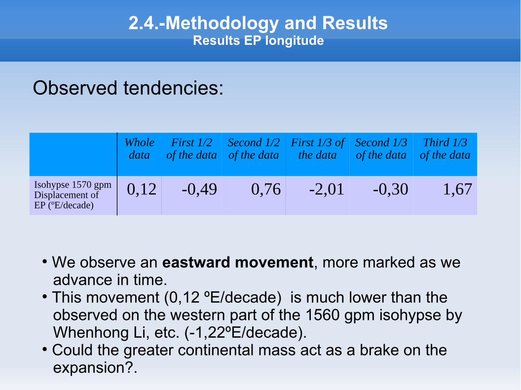
Isohypse 1570 gpm Displacement of EP (ºE/decade)

0,12 -0,49 0,76 -2,01 -0,30 1,67

Observed tendencies:

● We observe an eastward movement, more marked as we advance in time.

● This movement (0,12 ºE/decade) is much lower than the observed on the western part of the 1560 gpm isohypse by Whenhong Li, etc. (-1,22ºE/decade).

● Could the greater continental mass act as a brake on the expansion?.

2.4.-Methodology and ResultsResults NP latitude

2.4.-Methodology and ResultsResults NP latitude

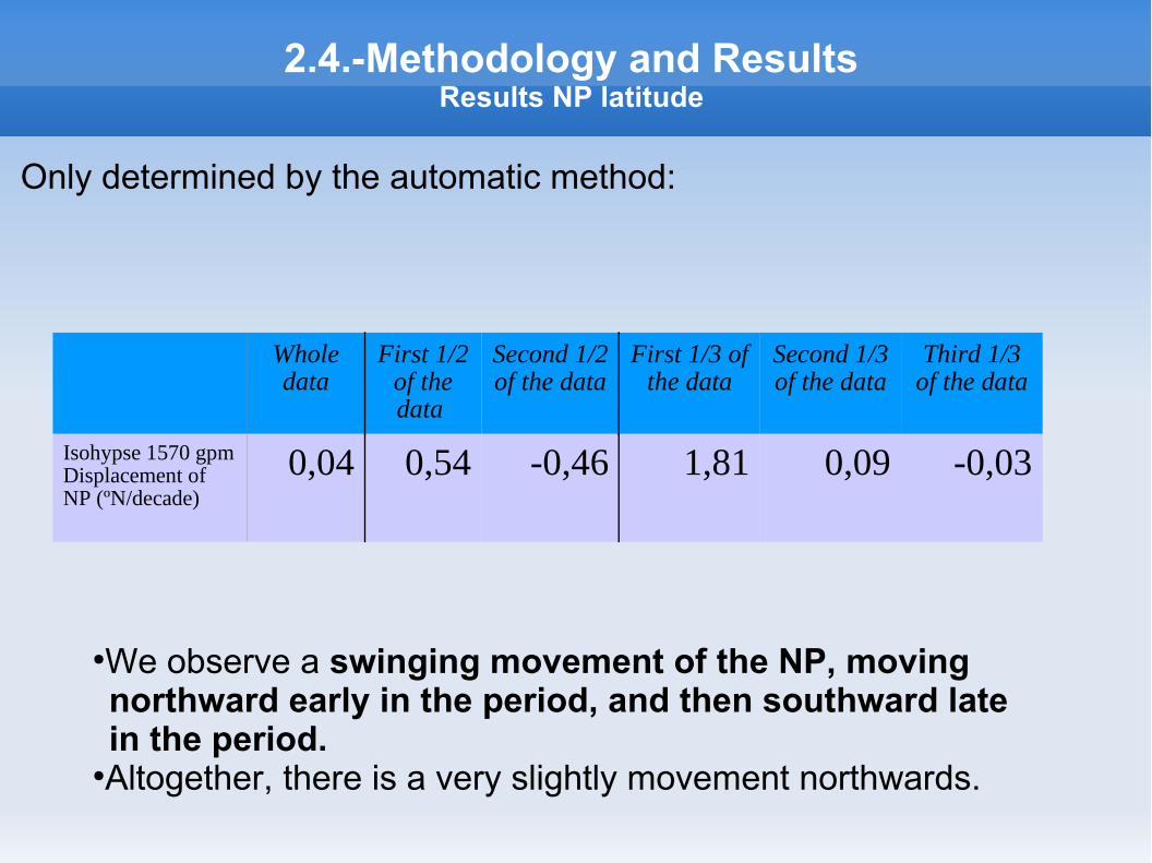
Only determined by the automatic method:

Whole data

First 1/2 of the data

Second 1/2 of the data

First 1/3 of the data

Second 1/3 of the data

Third 1/3 of the data

Isohypse 1570 gpm Displacement of NP (ºN/decade)

0,04 0,54 -0,46 1,81 0,09 -0,03

●We observe a swinging movement of the NP, moving northward early in the period, and then southward late in the period.

●Altogether, there is a very slightly movement northwards.

2.5.-Conclusion (I)

I have observed the intensification of the Maximum and eastward displacement of the easternmost point of 1570 mgp isohypse in the past, in summer time (JJA).

It is interesting to confirm this tendency with climate models projections data.

In the following page, we present an example of eight models that show a similar increasing tendency.

2.5.-Conclusion (II)

For this, we use projections from some RCM of ENSEMBLES PROJECT. RCMs don't have extension enough for containing the whole anticyclone or to properly deal with the 1570 gpm isohypse, so we do not calculate the intensity of the maximum, nor the NP or the EP, but can obtain the geopotential height at a fixed location (39.75 N, -14.74 E) included in the RCMs.

2.5.-Conclusion (II)

●Aladin_ARPEGE seems to be the model that best conforms with the variable we are studying.●It has also the greatest slope in its whole period.●All models have a positive slope in their whole period.●All means of all quarter-centuries are greater than the one in the reference sub-period.●Each mean of each quarter-century sub-period is greater than the precedent quarter-century sub-period, except for the two last models nested in ECHAM5-r3.

●However, models nested in ECHAM5-r3 predict the highest geopotential heights at the end of the century.

ERA40 0.26 0.26 1551.05 1558.77 0.18 1.67 1543.90 1549.37 1552.70 1560.93 1563.40

HadRM3Q0_HadCM3Q0 0.08 1.11 1518.76 1521.27 1523.66 1528.45 1531.40RACMO2_ECHAM5-r3 1.09 1.02 1562.54 1566.04 1566.11 1571.46 1574.99RCA3_HadCM3Q16 1.10 0.91 1512.04 1514.29 1515.55 1520.99 1521.88REMO_ECHAM5-r3 1.37 1.03 1552.33 1555.08 1554.69 1561.11 1564.22RegCM3_ECHAM5-r3 1.40 0.99 1552.67 1556.12 1556.12 1561.16 1564.63PROMES_HadCM3Q0 -1.26 0.58 1530.22 1533.91 1535.79RCA_HadCM3Q3 1.92 1.61 1489.84 1494.19 1499.47 1503.53 1508.71

Model

Slope in ERA40 Period

(1958-2002)

Slope in the whole period of

each model

Mean of reference

Sub-period(1961-2000)

Mean of sub-period 2001-2025

Mean of sub-period 2026-2050

Mean of sub-period 2051-2075

Mean of sub-period 2076-2100

NaN NaN NaNAladin_ARPEGE

NaN NaN

Models ordered by absolute value of difference between their slopes and the slope of ERA40, of the tendency line in the period of ERA40 (see last page).

Slopes are in m/decade and means are in m, except for ERA40 and Aladin_ARPEGE, which are in gpm/decade and gpm.

3. Interpolation to common grid

Objective. Interpolation to common grid of data from Ensembles Project.

– Grid area: 34ºN, -12ºE, 47ºN, 6,5ºE

– Grid resolution: 0.25ºx0.25º

– Interpolated periods: 1961-2000, 2011-2040, 2041-2070, 2071-2100.

Data Source.

– Five regional models: HadRM3Q0, HadRM3Q3, HadRM3Q16, CLM, PROMES.

– Daily means.

3. Interpolation to common grid

Methodology. InterIrr2Reg (Petra Ramos Calzado, Estudios y Desarrollos, Sevilla).

– Data input has to be pre-processed (ncatted, calendar).

– InterIrr2Reg works taking pieces of data as input and generates pieces as output, which has to be ensembled.

– This all has been done in Python.

– The tasks has been parallelized using the library Parallel Python www.parallelpython.com

3. Interpolation to common grid

Results.Generated data can be found at www.aemet.es, Servicios climáticos → Cambio climático → Datos numéricos → Servicio de Escenarios Climáticos de la AEMET → TÉCNICAS DINÁMICAS → PROYECTO ENSEMBLES → Descargar Datos, and then, select appropriate regional model.

PROMES is still awaiting.Development of quality control scripts.

4. Generation of graphics of evolution of seven variables

Objective: Generation of graphics of evolution for seven meteorological variables in spain, with data from regional climate models from the Ensembles Project. Also, csv files with data are generated.The variables are:● Total runoff (mrro = surface runoff + deep runoff)● Evaporation (evspsbl)● Total cloudiness fraction (clt)● 10-meter U wind (uas)● 10-meter V wind (vas)● 10-meter wind speed (wss)● 10-meter daily max. wind speed incl. gust (wsgsmax)

4. Generation of graphics4.1 Kinds of graphics

Two broader types of graphics:Time evolution.Spatial distribution (maps). In three periods:

1961-1990, 2046-2065, 2081-2098.

Showing three statistics:ValuesAnomaliesRelative anomalies

Domains:Spatial: Peninsula and CCAA.Temporal: Annual and seasonal.

4. Generation of graphics4.2 Data source

Ensembles project.Monthly means of daily means.SRESA1B.0.25ºx0.25ºRT2B experiment.Data are pre-processed to achieve quality.

4. Generation of graphics4.2 Methodology

Download dataTest and pre-process data.Cut out to Peninsula and Baleares.Time evolution graphics:

– Select control (1961-1990) and projection (2010-2100) periods.

– Apply mask for Peninsula and CCAA.– Calculate annual mean and seasonal mean in

each year.– Calculate spatial mean in each region.– Graph with R package.

4. Generation of graphics4.2 Methodology

Download dataTest and pre-process data.Cut out to Peninsula and Baleares.Spatial distribution (maps) graphics:

– Select control (1961-1990) and proyection (2046-2065 and 2081-2098) periods.

– Calculate time mean for each model in each period, annual and seasonal.

– Calculate ensemble mean of all models with standard deviation.

– Calculate anomalies and relative anomalies from ensemble means, with standard deviations.

4. Generation of graphics4.2 Methodology

This all has been done:In Bash scripts calling (mainly):

– Cdo– Ncdump

In Fortan programs using the Magics library.

4. Generation of graphics4.2 Results*. Sample images.

The graphics and csv files can be seen and downloaded at intranet of Aemet.

Total runoff, Peninsula, time evolution, anomaly:

4. Generation of graphics4.2 Results. Sample images.

Evaporation, 2081-2098 annual mean, anomaly:

4. Generation of graphics4.2 Results. Sample images.

Evaporation, 2081-2098 annual mean, standard deviation of anomaly:

4. Generation of graphics4.2 Conclusions

Total runoff:General downward tendency in XXI century,

strongest in high mountain areas and Galicia.

Evaporation:General downward tendency.Most important exceptions: Upward tendency in high

mountain regions.

4. Generation of graphics4.2 Conclusions

Evaporation:General downward tendency.Most important exeptions: Upward tendency in high

mountain regions.

Total cloudness (Fraction):General downward tendency (coherent with

precipitation diminution and temperature rise), except in winter for disparate regions like Andalucía and Basque Country.

4. Generation of graphics4.2 Conclusions

10-meter U wind and 10-meter V wind:General tendency: more easterly and less westerly.

And more southerly and less northerly.Anomalies are very small (~ 0.2 m/s).

10-meter wind speed and 10-meter daily max. wind speed incl. gust:General tendency: downward for all wind variables.Exception: summer, upward tendency. Difficult to

explain. Perhaps, higher temperatures implies more energy for winter generation.

Anomalies are very small (~ 0.2 m/s).

5. Current work

ADAPTATION AND IMPROVEMENT OF A STATISTICAL SEASONAL FORECASTING

MODEL

Objective: to put in work a (statistical) seasonal forecasting model for Spain.

Technical manager: Ernesto Rodríguez Camino

5. Current work

Source:

An adaptive multi-regressive method for summer seasonal forecast in the Mediterranean area. Pasqui M., Genesio L., Crisci A., Primicerio J., Benedetti R. and Maracchi G. CNR - IBIMET; 87th AMS Annual Meeting/ 13 January - 16 January 2007, Texas

5. Seasonal forecasting modelMethodology

Search for indices and teleconnections not yet implemented in the program of Ibimet:

– SAI

– PNA

– Arctic ice cover.

– Etc.Install programs and libraries needed by the

program:

– UV-CDAT

Thanks for your attention