Graduate Program in Engineering and Technology Management

Introduction to Simulation

Aslı Sencer

Aslı Sencer 2

Simulation

– Very broad term – methods and applications to imitate or mimic real systems, usually via computer

Applies in many fields and industries Very popular and powerful method

3

Advantages of Simulation

Simulation can tolerate complex systems where analytical solution is not available.

Allows uncertainty, nonstationarity in modeling unlike analytical models

Allows working with hazardous systems Often cheaper to work with the simulated system Can be quicker to get results when simulated

system is experimented.

Aslı Sencer

4

The Bad News

Don’t get exact answers, only approximations, estimates

Requires statistical design and analysis of simulation experiments

Requires simulation expert and compatibility with a simulation software

Softwares and required hardware might be costly Simulation modeling can sometimes be time

consuming.

Aslı Sencer

5

Different Kinds of Simulation Static vs. Dynamic

Does time have a role in the model?

Continuous-change vs. Discrete-change Can the “state” change continuously or only at

discrete points in time?

Deterministic vs. Stochastic Is everything for sure or is there uncertainty?

Aslı Sencer

6

Using Computers to Simulate

General-purpose languages (C, C++, Visual Basic)

Simulation softwares, simulators Subroutines for list processing, bookkeeping, time

advance Widely distributed, widely modified

Spreadsheets Usually static models Financial scenarios, distribution sampling, etc.

Aslı Sencer

7

Simulation Languages and Simulators Simulation languages

GPSS, SIMSCRIPT, SLAM, SIMAN Provides flexibility in programming Syntax knowledge is required

High-level simulators GPSS/H, Automod, Slamsystem, ARENA, Promodel Limited flexibility — model validity? Very easy, graphical interface, no syntax required Domain-restricted (manufacturing, communications)

Aslı Sencer

8

When Simulations are Used

The early years (1950s-1960s) Very expensive, specialized tool to use Required big computers, special training Mostly in FORTRAN (or even Assembler)

The formative years (1970s-early 1980s) Computers got faster, cheaper Value of simulation more widely recognized Simulation software improved, but they were still languages to

be learned, typed, batch processed

Aslı Sencer

9

When Simulations are Used (cont’d.)

The recent past (late 1980s-1990s) Microcomputer power, developments in softwares Wider acceptance across more areas

Traditional manufacturing applications Services Health care “Business processes”

Still mostly in large firms Often a simulation is part of the “specs”

Aslı Sencer

10

When Simulations are Used (cont’d.)

The present Proliferating into smaller firms Becoming a standard tool Being used earlier in design phase Real-time control

The future Exploiting interoperability of operating systems Specialized “templates” for industries, firms Automated statistical design, analysis

Aslı Sencer

11

Popularity of Simulation Consistently ranked as the most useful, popular tool in the

broader area of operations research / management science 1979: Survey 137 large firms, which methods used?

1. Statistical analysis (93% used it)2. Simulation (84%)3. Followed by LP, PERT/CPM, inventory theory, NLP,

1980: (A)IIE O.R. division members First in utility and interest — simulation First in familiarity — LP (simulation was second)

1983, 1989, 1993: Heavy use of simulation consistently reported

1. Statistical analysis 2. SimulationAslı Sencer

12

Today: Popular Topics

Real time simulationWeb based simulationOptimization using simulation

Aslı Sencer

13

Simulation Process

Develop a conceptual model of the system Define the system, goals, objectives, decision

variables, output measures, input variables and parameters.

Input data analysis: Collect data from the real system, obtain probability

distributions of the input parameters by statistical analysis

Build the simulation model: Develop the model in the computer using a HLPL, a

simulation language or a simulation software

Aslı Sencer

14

Simulation Process (cont’d.)

Output Data Analysis: Run the simulation several times and apply statistical

analysis of the ouput data to estimate the performance measures

Verification and Validation of the Model: Verification: Ensuring that the model is free from

logical errors. It does what it is intended to do. Validation: Ensuring that the model is a valid

representation of the whole system. Model outputs are compared with the real system outputs.

Aslı Sencer

15

Simulation Process (cont’d.)

Analyze alternative strategies on the validated simulation model. Use features like Animation Optimization Experimental Design

Sensitivity analysis: How sensitive is the performance measure to the

changes in the input parameters? Is the model robust?

Aslı Sencer

16

Static Simulation:Monte-Carlo Simulation Static Simulation with no time dimension. Experiments are made by a simulation model to estimate

the probability distribution of an outcome variable, that depends on several input variables.

Used the evaluate the expected impact of policy changes and risk involved in decision making.

Ex: What is the probability that 3-year profit will be less than a required amount?

Ex: If the daily order quantity is 100 in a newsboy problem, what is his expected daily cost? (actually we learned how to answer this question analytically)

Aslı Sencer

Example: Estimation of the Area

17

How do we estimate the area of a lake?

a

b

Estimate p by shooting arrows!Consider the experiement:Shoot an arrow into the rectangleEstimate of p = # hits in the lake / # shoots

Let p=area of lake/area of rectangleArea of lake= p. (ab)

. . ..... . . . . .. . . . . . . . . .. . .

Aslı Sencer

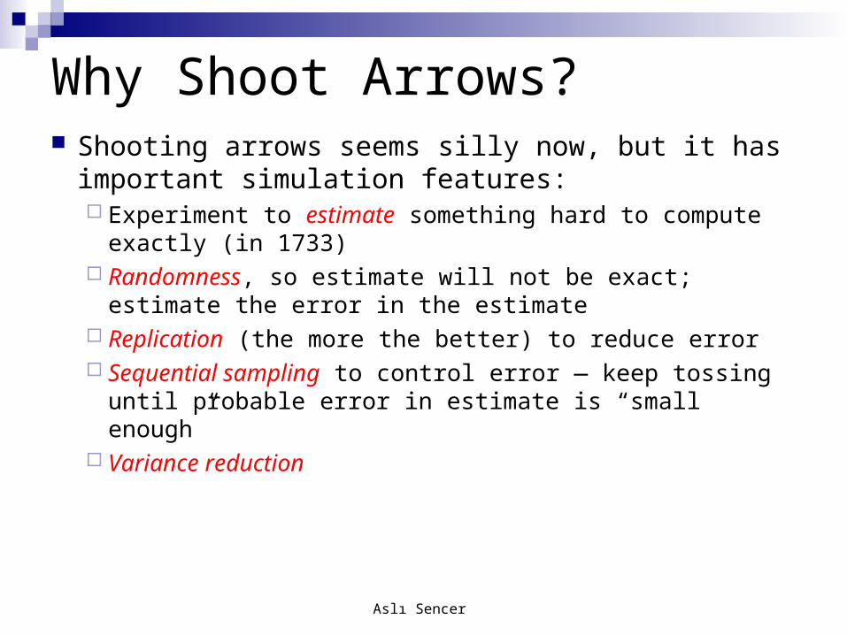
Why Shoot Arrows? Shooting arrows seems silly now, but it has

important simulation features: Experiment to estimate something hard to compute

exactly (in 1733) Randomness, so estimate will not be exact; estimate the

error in the estimate Replication (the more the better) to reduce error Sequential sampling to control error — keep tossing until

probable error in estimate is “small enough” Variance reduction

Aslı Sencer

19

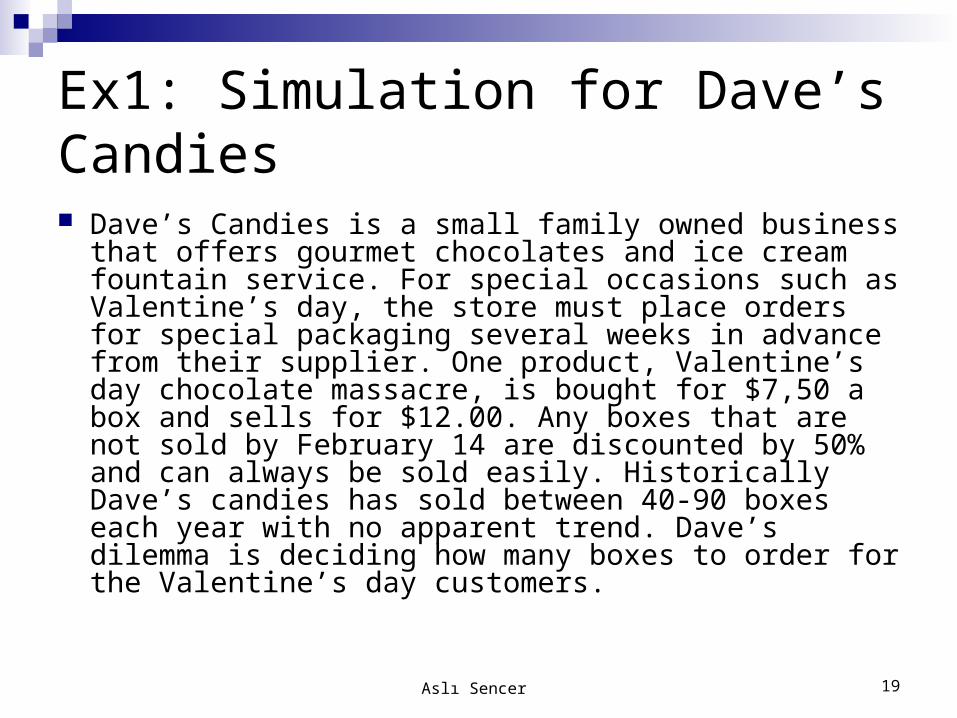
Ex1: Simulation for Dave’s Candies

Dave’s Candies is a small family owned business that offers gourmet chocolates and ice cream fountain service. For special occasions such as Valentine’s day, the store must place orders for special packaging several weeks in advance from their supplier. One product, Valentine’s day chocolate massacre, is bought for $7,50 a box and sells for $12.00. Any boxes that are not sold by February 14 are discounted by 50% and can always be sold easily. Historically Dave’s candies has sold between 40-90 boxes each year with no apparent trend. Dave’s dilemma is deciding how many boxes to order for the Valentine’s day customers.

Aslı Sencer

20

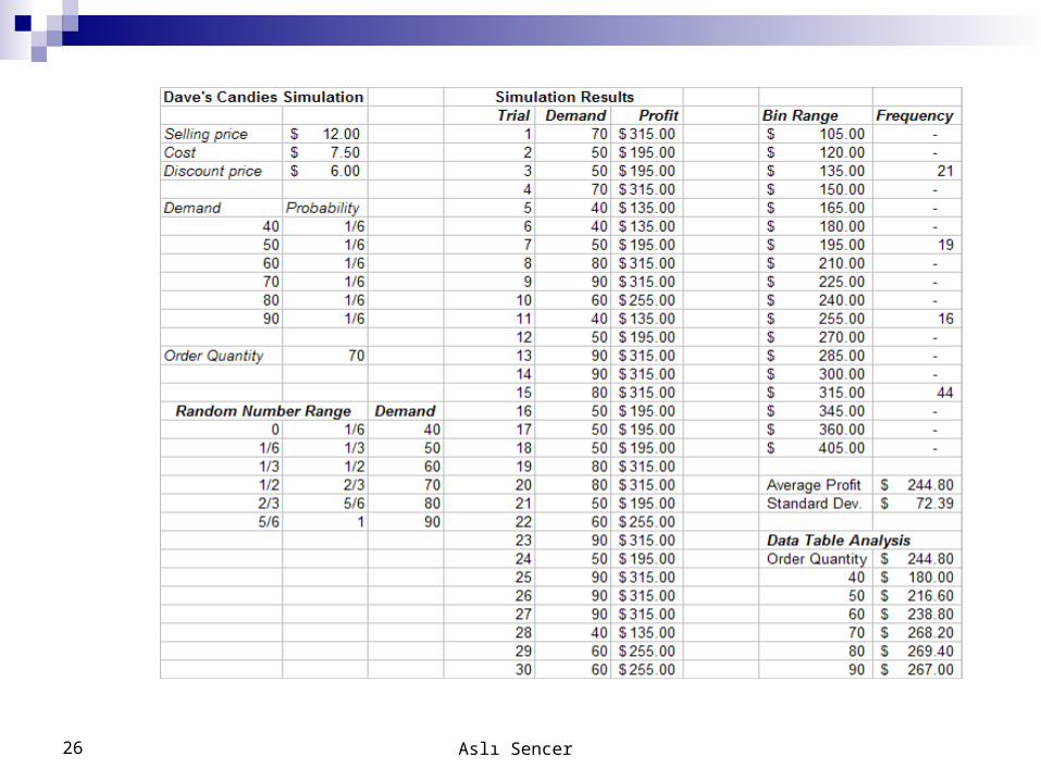
Ex1: Dave's Candies Simulation

If the order quantity, Q is 70, what is the expected profit?Selling price=$12Cost=$7.50Discount price=$6 If D<Q

Profit=selling price*D - cost*Q + discount price*(Q-D) D>Q Profit=selling price*Q-cost*Q

Aslı Sencer

Probability Distribution for Demand

Year Demand

2009 90

2008 80

2007 50

2006 60

2005 40

2004 70

2003 90

. .

. .

Demand Distribution

Demand

(xi, i=1,...,6)

Probability

P(Demand=xi)

40 1/6

50 1/6

60 1/6

70 1/6

80 1/6

90 1/6

Aslı Sencer

Generating Demands Using Random Numbers

During simulation we need to generate demands so that the long run frequencies are identical to the probability distribution found.

Random numbers are used for this purpose. Each random number is used to generate a demand.

Excel generates random numbers between 0-1. These numbers are uniformly distributed between 0-1.

Random numbers

0.12878

0.43483

0.87643

0.65711

0.03742

0.46839

0.04212

0.89900

Aslı Sencer

Generating random demands:Inverse transformation technique

23

P(demand=xi)

(xi)

40 50 60 70 80 90

1/6

P(demand<=xi)

(xi)

40 50 60 70 80 90

1

5/6

4/6

3/6

2/6

1/6

U1

D1=80

U2

D2=50

1. Generate U~UNIFORM(0,1)2. Let U=P(Demand<=D) then D=P-1(U)

Aslı Sencer

24

Generating Demands

Demand

(xi)

Probability

P(Demand=xi)

Cumulative Probability

P(Demand<=xi)Random numbers

40 1/6 1/6 [0-1/6]

50 1/6 2/6 (1/6-2/6]

60 1/6 3/6 (2/6-3/6]

70 1/6 4/6 (3/6-4/6]

80 1/6 5/6 (4/6-5/6]

90 1/6 1 (5/6-1]

Aslı Sencer

25

Ex1: Simulation in Excel for Dave’s CandiesUse the following excel functions to generate a random demand with a given distribution function.

RAND(): Generates a random number which is uniformly distributed between 0-1.VLOOKUP(value, table range, column #): looks up a value in a table to detremine a random demand.IF(condition, value if true, value if false): Used to calculate the total profit according to the random demand.

Aslı Sencer

26 Aslı Sencer