THE GROWH AND YlELD OF TEAK , Z

(Tectona grandis Limi F.)

THOMPSON K. NUNIFU a

A Graduate Thesis Submitted

In Partial Fulfilment of the Requirements

For the Degree of Master of Science in Forestry

Faculty of Forestry

Lakehead University

Thunder Bay, Ontario

December f997

National Library 1*1 of Canada Bibliothèque nationale du Canada

Acquisitions and Acquisitions et Bibliographie Services services bibliographiques

395 Wellington Street 395. rue Wellington Ottawa ON K1A ON4 Ottawa ON KIA ON4 Canada Canada

The author has granted a non- L'auteur a accordé une licence non exclusive licence allowing the exclusive permettant à la National Library of Canada to Bibliothèque nationale du Canada de reproduce, loan, distri'bute or sell reproduire, prêter, distribuer ou copies of this thesis in microform, vendre des copies de cette thèse sous paper or electronic formats. la fonne de microfiche/nlm, de

reproduction sur papier ou sur format électronique.

The author retains ownership of the L'auteur conserve la propriété du copyright in this thesis. Neither the droit d'auteur qui protège cette thèse. thesis nor substantial extracts fkom it Ni la thèse ni des extraits substantiels may be printed or otheMrise de celle-ci ne doivent être imprimés reproduced without the author's ou autrement reproduits sans son permission. autorisation,

A CAUTION TO THE READER

This MscF thesis has been through a semi-forma1 process of review and

cornments by at least two faculty members.

It is made available for loan by the faculty for the purpose of advancing the

practice of professional and scientific forestry.

The reader should realize that opinions expressed in this document are the

opinions and conclusions of the student and do not necessarily reflect the

opinions of either the supervisor, the faculty of the University

ABSTRACT

Nunifu, K. T. 1997. The growth and yield of teak (Tectona grandis Linn F.) plantations in Northem Ghana 1 O1 pp. MScF Thesis, Faculty of Forestry, Lakehead University. Advisor: Dr. H. G. Murchison.

Key Words: Biomass, Biomass equations. Northern Ghana, Teak, Tectona grandis, Volume Tables, Yield rnodels.

Teak (Tectona grandis Linn F.) is a popular exotic species in Ghana. widely grown in industrial plantations and small scale community woodlots. In spite of its importance, Iimited information exists on the growth and yield of this species. Presented here are the results of a preliminary study airned at assessing the growth and yield potential and developing provisional yield models for the management of teak in Northem Ghana. Data were collected from 100 temporary sample plots from plantations in this region, ranging in ages from 3 to 40 years. Local, standard and stand volume equations and tables were constructed from the data. Additive above ground biomass and site index equations, and provisional empirical yield models were also developed and presented. Site index curves were used to classify teak plantations in the region into site classes 1, II and III, in order of decreasing productivity. The assessrnent of growth and yield revealed the potential for growing teak to acceptable timber size on good sites. Yield functions, indicate that teak can be grown on biologically optimum rotations of 31, 38 and 48 years on site classes I , II and III respectively. The diameter distribution was modelled by the three-parameter Weibull function, using the maximum likelihood and the percentile parameter estimators. The diameter distribution showed positive skewness indicating there are more trees in smaller diameter classes. Initial planting spacing of 2 by 2 m could be reduced to accommodate inlial mortality and to achieve optimum stocking levels in order to improve form and timber quality.

TABLE OF CONTENTS

Page

ABSTRACT

LIST OF TABLES

FIGURES

ACKNOVVLEDGEMENTS

1 .O INTRODUCTION

2.0 LITERATURE REVIEW

3.0 MATERIALS AND METHODS

3.1 THE STUDY AREA

3.1.1 The Natural Vegetation Zones

of Ghana

3.1.2 The Guinea Savanna Vegetation

zone

3.2 DATA COLLECTION

3.3 DATA ANALYSIS

3.3.1 Volume Estimations

3.3.2 Biomass Computations

3.3.3 Yield Models

3.3.4 Diameter Distribution Models

i i

vi

vii

viii

1

4.0 RESULTS

4.1 DIAMETER AND HEIGHT GROWH

4.2 VOLUME ESTIMATIONS

4.3 BIOMASS EQUATIONS AND TABLES

4.4 YlELD MODELS AND TABLES

5.0 DISCUSSION

5.1 ASSESSMENT OF GROWH AND YlELD

OF TEAK IN NORTHERN GHANA

5.2 VOLUME EQUATDNS AND TABLES

5.3 BIOMASS EQUATlONS AND TABLES.

5.4 YlELD MODELS AND TABLES.

5.5 DIAMETER DISTRIBUTION MODELS

6.0 CONCLUSIONS AND RECOMMENDATIONS

7.0 LITERATURE CITED

APPENDIX 1 SUMMARIES OF STAND CHARACTERISTICS BY PLANTATIONS

APPENDIX II COMPARISON OF STAND VOLUME ESTIMATES BY TWO-STAGE SIMPLE RANDOM SAMPLING, PROBABILITY PROPORTIONAL TO BASAL AREA, AND THE USE OF VOLUME TABLES

APPENDIX III ABOVEGROUND BIOMASS ESTIMATES IN TONNES PER HECTARE

APPENDIX IV LIST OF STANDARD MODELS FOR VOLUME TABLE CONSTRUCTION

APPENDIX V STANDARD VOLUME TABLES FOR TEAK IN PLANTATIONS NORTHERN GHANA

APPENDlX VI

APPENDIX VI1

APPENDIX Vltl

APPENDIX IX

APPENDIX X

APPENDIX XI

APPENDIX XII

APPENDIX XII1

APPENDIX XIX

LOCAL VOLUME TABLE FOR TEAK PLANTATIONS IN NORTHERN GHANA

ABOVE GROUND BIOMASS TABLES FOR TEAK PLANTATIONS IN NORTHERN GHANA

MEAN OVEN DRY BIOMASS AS PROPORTIONS OF FRESH BIOMASS OF THE ABOVEGROUND TREE COMPONENTS

SUMMARY OF GROVVTH AND YIELD DATA FROM TEAK PLANTATIONS IN THE OFFINSO DISTRICT IN THE HlGH FOREST ZONE OF GHANA

YIELD TABLES FOR TEAK PLANTATIONS IN NORTHERN GHANA

OBSERVED AND PREDICTED DIAMETER CLASS FREQUENCIES BY AGE CLASSES

SITE INDEX CURVES FOR TEAK PLANTATIONS IN NORTHERN GHANA

VOLUME GROWH CURVES FOR TEAK PLANTATIONS IN NORTHERN GHANA

DERIVATION OF THE CUMULATIVE VVEIBULL DISTRIBUTION FUNCTION FROM THE WEIBULL PROBABILITY DENSITY FUNCTION

vi

LIST OF TABLES

Table 1. The Summary Statistics for diameter and height rneasurements

Table 2. The estirnates of the Weibull parameters by the maximum likelihood (MLE) and the percentile methods 53

Table 3. Coefficients and standard errors of the heig ht-d b h eq uation

Table 4. Coefficients of local volume equations by site class

Table 5. Absolute and artificial form factors and fom quotients for teak

Table 6- Coefficients of additive biornass models

Table 7. Regression coefficients for component yield models for plantation teak in Northem Ghana

FIGURES

Page

Figure 1. The Study Area 34

Figure 2. The Natural Vegetation Zones of Ghana. 37

Figure 3. The scatterplot of the standardized residuals from the double entry volume equation against predicted values. 55

Figure 4. The graph of top height against age from site class I in the study area, site class III Indian yield tables and site class II Trinidad yield table.

I wish to thank Dr. H. G. Murchison, my major advisor, Dr. Ulf. Runesson

and Mr. Richie Clarke for their support and guidance by way of constructive

criticism, in preparing this thesis. Special thanks to the Ghana forestry Department

and particularly to James Amaligu, a technical officer, for the cooperation and

support offered me during the data coilection. I will also like to acknowledge the

assistance of the Canadian International Development Agency (CIDA) in funding

my graduate studies at Lakehead University and particularly, this thesis project.

I must not forget my former room mates; Messrs David Nanang and

Hypolite Bayor for the company, fun and inspiration I got from them during the

early stages of my graduate studies. Many thanks to Mrs Crescentia Dakubo,

Messrs Francis Salifu and Ben Donkor, their company and contributions in diverse

ways have been very essential for the success of this thesis. My other Ghanaian

colleagues: Ms Agnes Apusigah, Ms Nana-Ama Asare, Ms Bernice Mensah, Ms

Mercy Boafo, Messrs Anthony Eshun, Isaac Arnponsah, Kofi Poku, Aaron Ankudy

and Yohanes Honu, have been very supportive in one way or the other, and to

them I Say many thanks.

Special thanks to Dr. Moanami of the Department of Econornics, whose

contribution has not only been important for the development of this thesis, but to

my entire career. Finally, I wish to acknowledge the support of special friends:

Tigist Abebe, Ayot Felix and her sister Martha Ottoviano.

To My wife Ruth Nunifu and Our two kids; Yoobat and Suguruman Nunifu,

for their love, patience and the hard times they had to go through without me.

THE GROWTH AND YlELD OF TEAK (Tectona gandis Linn F.) PLANTATIONS IN NORTHERN GHANA.

1 .O INTRODUCTION

Teak (Tectona grandis Linn F. Verbenaceae) is one of the most important

plantation species both in the high forest and the savannah zones of Ghana. The

species was introduced into Ghana between 1900 and 191 0 (FA0 and UNEP

1981). Teak has since acclimatized well and has been widely grown in both

industrial plantations and small community woodlots.

Large scale plantations of teak in Ghana started in the late 1960s, under a

plantation programme that was initiated wlh the help of the Food and Agriculture

Organization (FAO) of the United Nations (Prah 1994). These plantations,

estimated to cover about 45,000 ha (Drechsel and Zech 1994) were to supplement

the supply of wood products from the indigenous natural forests.

Teak, a high quality deciduous timber species, native to Peninsular India, Burma

and Indonesia, has gained importance in Ghana in recent times as a source of

electffc transmission poles for the rural electrification project. A further increase

in teak plantations occurred following the establishment of a 5-year rural

afforestation programme in 1989 under the Ghana Forestry Department, which

2

saw an increase in the extent of existing as well as the establishment of new

plantations in Northern Ghana. Apart from electric and telep hone transmission

poles, the tree is also valued by small scale famers and locai communities as

poles for construction, fencing, rafters, fuel wood, stakes and wind breaks. It has

also become an important source of income for small scale farmers who plant the

species on their farms.

There is a considerable potential for growing teak to timber size on good soils in

Northem Ghana (FA0 and UNEP 1987) and the economic benefits are

undisputed. However, local knowledge on the growth and yield characteristics of

the species which will help in realising this potential and assist in making important

management decisions is still lacking.

This study was therefore designed as a preliminary investigation, aimed at

assessing growth and yield, developing provisional growth and yield models and

tables for management, and to serve as a basis for future studies into the growth

and yield of teak in Northern Ghana. The specific objectives are:

1) to assess the growth and yield of teak,

2) to develop volume and biomass tables for teak,

3) to develop provisional yield functions and tables for teak in plantations

in Northern Ghana.

2.1 CRITICAL SILVICS OF TEAK

2.1.1 General Description and Natural Distribution of teak

Teak, also known comrnercially as teek (Spanish) belongs to the family

Verbenaceae. It grows naturally in Southern Asia, from the Indian Subcontinent,

through Buma and Thailand to Laos, approximately 9' and 25ON latitude and 73"

to 103OE longitude (Troup 1921). As an exotic species, teak grows in several parts

of the worid. According to Hedegart (1 976), the wide distribution of teak attests to

the fact that, teak can survive and grow in a wide range of climatic and edaphic

conditions. It is generally drought and heat resistant.

Teak Vary in size according to locality and conditions of growth. On favourable

sites, it may reach a height of about 40 to 45 m, with a clear bole of up to 25 or 27

m, and a diameter of between 1.8 and 2.4 m (Farmer 1972). According to Kadambi

(1972), records from Thailand reported a teak tree, claimed to be the worlds

largest tree (1965), with approximately 22 feet (6.6 m) diameter at breast height

(dbh) and 151 feet (45 rn) total height. In drier regions, trees are generally small.

The boles are generally straight, cylindrical and clear when Young, but tend to be

fluted and buttressed at the base when mature. They tend to fork when grown in

4

isolation, but are generally shade intolerant.

2.1.2 Site and Soil Reuuirement

Teak grows on a variety of geological formations and soils (Kadambi 1972, Seth

and Yadav 1959), but the quality of growth depends on the depth, structure,

porosity, drainage and moisture holding capacity of the soi1 (Kadambi 1972). Teak

grows best on deep, well drained and fertile soils with a neutral or acid pH

(Kadambi 1972, Watterson 1971), generally on elevations between 200 and 700

m, but exceptionally on elevations up to 1300 m above sea level (Troup 1921).

Wam tropical, moderately moist climate is best for teak growth. Optimum annual

rainfall for teak is 1200 to 1600 mm, but it endures rainfall as low as 500 mm and

as high as 5000 mm (FA0 1983, Hedegart 1976, Kadambi 1972, Troup 1921).

2.1.3 Establishment and Earlv Growth

Plantation grown teak is established using stump plants rather than direct sowing

of teak seeds which does not always give satisfactory results (Borota 1991).

Depending on desired product (fuelwood, poles, lumber or a mixture of products)

and the site quality, the inlial planting spacing generally range from 1.8 by 1.8 m

5

to about 3 by 3 rn (Kadarnbi 1972). When planted in taungyal, spacing could be

as wide as 4.5 rn between rows. Generally, on good soils, wider spacing is used.

This results in better diameter and height growth, and also reduces nursery,

planting and early thinning costs (Kadambi 1972). On sloping terrain, wider

spacings have been suggested to encourage ground cover and to avoid erosion

(Weaver 1 993).

Teak is generally shade intolerant but needs training for improved fom. Closer

than the normal planting spacing is sometirnes adapted to ensure quick canopy

closure, thereby achieving training and reducing weeding cost (Adegbeihn 1982,

Kadam bi 1 972). This practice necessitates early thinning .

The tirne of the first thinning is largely determined by site quality. Lowe (1976)

noted that although thinning may be delayed for 10 to 15 years after planting

without unduly affecting the growth potential of the final crop, very heavy thinning

becomes necessary if the growth of the final tree crop is to be maintained at

satisfactory levels.

The practice where by faners grow food crops with trees on the same piece of land to help raise the tree crop with the agreement that, food crop cornponent be removed when the tree crop gets established.

2.1 -4 Growth and Yield

Teak is generally fast growing when Young, but it's overall growth rates on rotation

basis is not outstanding (FA0 1956). It is considered rnoderate to fast growing

(Briscoe and Ybarra-Conorodo 1971). A study of the standing biomass of teak in

India, showed height growth to be most rapid between 1 0 and 50 years after which

it declined (Weaver 1993).

The rotation of teak in lndia is a function of forest type and management systems

(Ghosh and Singh 1981). Plantation crops have rotations between 50 and 80

years, whereas in areas where teak occurs in mixed stands, rotation is about 70

to 80 years. Coppice systems or coppice with standards have rotations of between

40 and 60 years (Wieaver 1993).

FA0 (1985) quotes the peak ages for the mean annual volume increment at 50

and 75 years respectively, for site classes I and II in Kerala, India, based on

stemwood volume. In lndian yield tables for teak (Laurie and Ram 1940). the

maximum total volume growth occur at ages between 5 and 15 years depending

on site class. Similar estimates in Trinidad (Miller 1969) are bebveen 7 and 12

years. At Mtibwa, Tanzania, Malende and Temu (1 990) estimated the peak ages

of mean and current annual incrernents for teak to be at 42 and 55 years

respectively.

7

At base age 20, the site index for teak was estimated by Malende and Temu

(1 990) to be between 16 and 25 m. In Miller (1 969), the estimate is between 15

and 23 m. Akindele's (1 991) estimate for Northwestern Nigeria was between 10

and 29 m. At the same base age, figures from Laurie and Ram (1 940) ranged frorn

28 m for site class I to 12 m for site class V. Similar results have been reported by

Keogh (1982), Frîday (1 987), and Drechsel and Zeck (1 994). In Ghana, a similar

study for teak in the high forest zone reported indices ranging from 17 m to 26 m

(Anonymous 1992).

Logu et ai. (1988) estimated the above ground biornass production for teak to be

between 2.1 and 273 tlha for ages ranging from 5 to 97 years respectively. The

mean annual biornass increments was estimated to peak at between 10 and 40

years depending on site conditions.

2.2. SAMPLING FOR GROWH AND YIELD

2.2.1 Permanent and Serni-permanent Sample Plots

Permanent sample plots (PSPs) are considered the most reliable sources of data

for estimating and modelling growth and yield (Alder and Synott 1992). Apart from

individual tree increments, PSPs provide information on recruitments and mortality.

These estirnates may not be necessary for monitoring well managed plantations.

8

but are essential components of growth in mixed natural forests (Alder 1980, Alder

and Synott 1992)

PSPs are classified into experimental and passive monitoring plots (Vanclay et al.

1995, Alder and Synott 1992). Passive monitoring plots by definition are

constrained to existing conditions whereas experimental plots are established to

explore novel situations, particularly extreme treatments (Alder and Synott 1992)

such as varying intensities of thinning.

The process of obtaining data frorn PSPs to cover the entire rotation of a stand

takes a long time to complete and the stand may get destroyed by fire, disease or

other catastrophic agencies (Chapman and Meyer 1949). Besides, it has been

argued that, the more times a PSP is measured, the less information it provides

as compared with the previous rneasurement, unless it is growing into an age-site-

stand density stratum that has not been well sampled (Alder 1980). In this case,

sampling is more efficient if plots are replaced after a few re-measurements. This

is particularly true for plantations or even-aged forests (Alder 1980). Semi-

permanent plots offer the best alternative in this regard.

Semi-permanent plots are located in stands of different ages, covering the full

range of site condition, and remeasured for only a few tirnes at suitable intervals.

By the overlapping of the ages chosen, the trend of development is established

9

(Chapman and Meyer 1949). This method is particularly suitable for plantations or

even aged natural forests where records of planting or logging dates are available.

The general disadvantage of PSPs is the high cost of establishment and

maintenance. Plot size and sampling intensity is therefore, often low (Shiver and

Borders 1996, Sheil 1995). There is also the tendency of treating PSPs differently

when they are clearly rnarked for the purpose of re-locating them for

measurements. This brings into question, their representativeness of the

population.

2.2.2 Temporary Sample Plots

Temporary sample plots (TSPs) are primariiy used for estimating relationships that

are not time dependent (Alder 1980). They are used in static inventories to

estimate the amount of growing stock in relation to the land area. However, growth

can be estimated from TSPs by stem analysis if annual growth rings are present.

Based on the principle of cornparison of plots of different ages, TSPs can be used

to construct yield models (Chapman and Meyer 1949). Many plots of different

ages, covering different site condlions are measured and the averages for stands

of the same sites but different ages are combined into a curve, assumed to show

the trend of growth (Chaprnan and Meyer 1949). This way, TSPs are useful

10

alternatives to PSPs when there is an urgent need. However, many plots, covering

the range of site conditions are needed to accurately detemine the growth trend.

In recurrent inventory, growth is estimated from TSPs by the simple difference

between estimates of a stand or tree attribute on two successive occasions. The

standard error of this estimate is high since the estimates on the two occasions are

independent (Shiver and Borders 1996, Philip 1994, Schreuder et al. 1993,

Murchison 1989, Loetsch et al. 1973). TSPs however have the advantage of less

cost and hence pemits higher sampling intensity which can result in accurate

estimates.

2.2.3 Samplina with Partial Replacement

The development of this method of sampling in forestry goes back to Bickford

(1 956) and particulariy to Ware and Cunia (1962). who provided a unifying theory

for this method and compared it to different growth estimators (Shiver and Borders

1996). The basic aim of the theory was to provide estirnators for curent stand

volume and growth with improved precision.

In sampling with partial replacement (SPR) only a portion of the plots or units are

retained for re-rneasurements on the subsequent occasions. These are called the

matched plots and could be permanent or semi-permanent plots. In addition,

11

ternporary (or unrnatched) plots are established and are not re-measured. The

improvement in precision came first from a direct increase in sample size and

second from exploiting the correlation between the matched PSP and the

unmatched TSP estimates on both occasions.

The rnatched plots makes it possible to accurately estimate growth, mortality and

recruitments. Wth many more temporary plots, the estimate of the current growing

stock can be accurately determined. Moreover, the improved estimates of current

growing stock makes growth estimates even more precise (Shiver and Borders

1996). The problem with this inventory design is the choice of optimum

combination of matched and unmatched plots. A combination that minimizes cost

and standard error is often the ideal.

2.3 TREE VOLUME AND YlELD ESTIMATION

Several methods have been developed to estimate stand volume and yield, each

varying in degree of sophistication and precision depending on the complexity of

the system dealt with. For the purpose of this study, stand volume estimation by

the mean tree method and volume tables will be discussed in some detail.

12

2.3.1 The Mean Tree Method of Stand Volume Estimation

The underlying theory of this method is that, the volume obtained by careful

measurement of the tree of mean volume can be multiplied by the nurnber of trees

in the stand or plot to obtain the estimate of the stand or plot volume (Spurr 1952).

The rnost common approach is to obtain the average volume of sub-sarnple trees

in each plot as the plot mean tree volume. From this and the number of trees, the

volume of each plot is calculated and hence the volume per hectare. This

approach is in fact, two-stage sampling with the sub-sample trees constituting the

second stage sample.

The common problern with this method is the sub-sample size, which is usualiy

small, especially when sub-sample trees are to be felled for detailed

measurements. According to Philip (1994), a minimum sub-sample size of about

20 trees per plot is nomially needed to provide a precise estimate of the volume

of the mean tree. Philip (1994) suggested the pooling together of the sub-sample

trees of al1 plots to get a pooled tree of mean volume. He however warned that a

serious bias could result if different plots provide different numbers of trees in the

sub-sarnple and contain different sizes of trees.

Another approach is based on the assumpüon that, the tree of mean basal area

is also the tree of mean volume (Spurr 1952. Crow 1971). Although fairly good

13

results have been obtained by this method, especially when the tree of mean

basal area is also the tree of mean height, the fallacy of the basic assumption has

long been recognized (Spurr 1952). The mean tree in this case is a tree with

diameter as close as possible, to the quadratic mean diameter of a sarnple of trees

from the target stand. This tree is isolated and its volume carefully determined.

The ratio of the volume to basal area of the mean tree can be multiplied by the

total basal area of the plot to obtain plot volume estimate (Schreuder et a/. 1993).

2.3.2. Stand Volume Estimation usina Volume Tables

Since it is not possible to rneasure individual tree volume directly in the field, it

must be estimated by the use of auxiliary variables such as diameter and height

(Murchison 1984). The use of volume equations and tables which relate these

variables to tree volume offers speed and mnvenience in estimating stand volume.

There is no doubt therefore that, the use of volume tables is the most common

approach to estimating yield.

Volume tables may be constructed on the basis of single tree or stand volume.

Single tree volume tables predict volume per tree and stand volume tables predict

volume per unit area (usually per hectare) (Philip 1994). The single tree volume

tables can be distinguished into local (single entry), standard (double entry) and

fonn class (multiple entry) volume tables (Husch et al. 1982). Local volume tables

14

give tree volume in ternis of diameter at breast height (dbh) only. The terni local

is used because, such tables may generally be restricted to the local area for

which the height - dbh relationship that is hidden in the table is relevant (Husch et

al. 1982). Avery and Burkhart (1994) however noted that, the terms "localn and

"standardn as used to describe the single entry and the double entry volume

equations do not suggest the former is inferior to the latter.

Standard volume tables give the volume of the tree in terms of dbh and

merchantable or total height. These are normally prepared for single species, or

a group of species and specific localities (Husch et al. 1982). The third type, the

fom class volume tables give volume in terms of dbh, merchantable or total

height. and some measure of form such as Girard form class or absolute form

quotient (Spurr 1952, Husch et al. 1982, Avery and Burkhart 1994).

Single tree volume tables are generally prepared by three methods; the graphical,

alignrnent chart and the regression methods. The graphical method is the oldest

and requires less mathematical techniques (Spurr 1952). It is however

unsatisfactory as 1 is open to subjectivity and the error in estimated volume cannot

be measured (Philip 1994, Spurr 1952).

The alignment chart method is another old technique of volume table construction.

It was first introduced by Bruce and Reineke (1 931) to correct for curvilinearity in

15

multiple regression equations (Spurr 1952). It produces satisfactory results, though

there are several disadvantages associated with it (Spurr 1952). A common

disadvantage is, prepared base charts are needed which are not always available.

Moreover, the charts cannot be read very accurately and are subject to error

because of dimensional changes in the paper (Spurr 1952).

The graphical and the alignment chart methods have been generally discarded in

favour of mathernatical functions and models (Husch et ai. 1982). These methods

consist of measuring the volume of selected trees in a representative sample,

establishing a relationship between the measurernents taken on the tree and

volume (usually by regression analysis), choosing the best model and verifying the

accuracy of the tables constructed (Philip 1994).

In selecting trees for the construction of volume tables, there is the need to clearly

define the population. This could be by species, geographic location or age. Some

form of stratification becomes necessary if variation in tree size and growth

conditions is high (Demaerschalk and Kozak 1974, Marshall and Demaerschalk

1986). In plantations, age is a useful basis for stratification (Philip 1994).

The choice of appropriate model is based on adequacy of fit as dictated by least

squares regression assumptions; normality of regression residuals, uniformity of

variance across al1 predictor variables, and the independence of the predictor

16

variables and reg ression residuals.

These assumptions are hardly met in practice and often, sorne form of

transformation is necessary. Commonly, the logarithmic transformation is used,

but is shown to have some bias in prediction. Details of this bias and its correction

as proposed by Baskerville (1972), are presented in section 2.4.2. The most

common problem in volume table construction has been heteroscedasticity of

residuals. This is because, larger tree volumes tend to deviate more from the

regression line than smaller ones. Cunia (1964) proposed the use of weighted

least squares to correct for heteroscedasticity in volume table construction.

Once two or more models demonstrate adequacy of fit in ternis of these

assumptions, a number of methods exist for evaluating goodness of fit. The

common ones are; the coefficient of determination (R2), standard error of the

mean, Furnival index (Fumival 1962) and the mean square difference between

predicted and observed volumes (Schlaegel 1981 ). The Furnival index is

calculated as:

Where FI is the Furnival index, SE is the standard error of the fitted regression,

and GM, is the geornetric mean of the dependent variable. The best model is the

17

one wîth high coefficient of determination (R2), srnaIl standard error of the mean

in the measured units, and small Fumival index (Fumival 1961).

Stand volume tables are based on stand variables such as basal area, top height,

mean height and mean dbh. The most cornmon stand volume tables are based on

the regression of volume per hectare on stand basal area per hectare and some

rneasure of height representative of the crop; often the dominant or top height is

used (Philip 1994).

The rneasure of volume per hectare may be obtained by measuring a

representative sample h m the stand or by measuring the volumes of small plots

directly or indirectly by the use of individual tree volume tables. According to Philîp

(1994), the error of prediction in the latter case must be derived from the sum of

error from three sources; residual variance in the single volume table, residual

variance in the stand volume table and the variance in the sarnpling units

themselves. In the former case, only the last two sources of variance are included

in the error. The criteria for judging adequacy of fit is similar to those shown for

single tree volume tables.

18

2.4 FOREST BIOMASS AND YIELD ESTIMATION

The conventional measure of yield in forestry has been related to volume. This is

because of the use of tree stem for wood products such as lumber, plywood,

poles, pilings, pulp and paper (Aldred and Aiemdag 1988). the value of which are

closely related to volume. Consequently, mensuration has been primarily directed

towards developing techniques for expressing forest g rowth and productivity in

ternis of merchantable log volume (Young 1971).

In contrast however, in many established community forests in developing

countries, al1 the forest components are used - branches. foliage and stems

(Applegate et al. 1988). In such situations, biomass estimates are the most

suitable for quantifying products. By definition, biomass is the amount of living

organic matter accumulation on a unit area at a specifÏed point in tirne (Newbould

1967). This is nonally expressed in terms of fresh or oven dry weights on per unit

area bases. The usual measure of biomass in forestry has been the above ground

tree components, which are easily accessible. However, total tree biomass is

defined to include the under ground cornponents (roots).

There are two common techniques for estimating biomass in forestry; the mean

tree method and regression analysis. If available, specific gravity can be used to

convert volume tables into biomass tables.

2.4.1 The Mean Tree Method of Biomass Estimation.

The basic principle is similar to the mean tree method of stand volume estimation;

a tree of mean biornass is isolated and Ït's biomass carefhlly measured. The stand

biomass is then obtained by multiplying this esthate by the number of trees in the

stand. This is accomplished by obtaining estimates of stand attributes that

approximate those of the tree of mean biomass. Crow (1971) used different

measures of stand characteristics to determine the tree of rnean biomass, but

each was shown to have some amount of bias. Some of these are, the tree of

mean total height, tree of mean total height and diameter, tree of rnean diameter,

tree of mean basal area and tree of mean bole volume.

The dificulty of getting measures that closely approximate those of the tree of

mean biomass is the major disadvantage of this method. This results from high

variation in tree size, especially in natural stands. Baskerville (1965)

recornmended the use of a stand table approach in which estimates are based on

the weight of a mean tree within each diarneter class multiplied by the frequency

within the class.

20

2.4.2 Biomass Euuations and Tables.

Perhaps the most widely used and convenient method of quantifying forest

biomass is by the use of equations or the tables constnicted from them. According

to Applegate et a/. (1988), this is so because of the simpiicity in determining

estimates and the ease with which results can be applied. This method relates

easily measured variables such as the diameter and height to the component

biomass of the forest fractions (Baskerville 1972, Madgwick and Satoo 1975).

The principie upon which biomass equations are obtained may be simple; 1) fell

representative sample trees and take sub-samples for oven dry weight

determination, 2) extrapolate from the sub-samples to the whole component and

sum up the various components to obtain the total tree biomass, and 3) develop

a predictive mathematical model relating the easily measured variables to the

component biomass.

The problems however. are in: (i) selecting representative sample trees and parts,

(ii) developing an unbiased predictive model, and (iii) ensuring additivity of the

parts to equal the whole tree biomass (Philip 1994).

Aldred and Alemdag (1 988) noted that, selecting samples for biomass tables must

follow statistically defensible sampling rules to ensure that the population of

21

interest is properiy represented. Simple random sampling of trees or clusters of

trees in a highly varied population rnay not achieve the desired representation,

though this may be quite satisfactory for even-aged pure stands. In general, the

need for some form of stratification has been recommended for uneven-aged

mixed stands (Cunia 1979a).

Sub-sampling of the component fresh biomass is a necessity when trees are

large. in which case weighing al1 tree components become impossible. Reliable

sub-sampling rnethods have been proposed such as, randomised branch sampling

(Jessen 1955, Valentine and Hilton 1977) and importance sampling (Rubstein

1981). Valentine et al. (1984) presented a combination of these two sampling

methods for estimating above ground biornass, woody volume and minerai

contents and discusses the theory and principles. The method is shown tu be

efficient, provides unbias estimates and avoids the time consuming labourious task

of weighing the whole tree.

Most authors have found that total biomass may be predicted satisfactorily from

diameter at breast height (dbh) (eg. Cunia and Briggs 1984). These equations

commonly take the fom of a quadratic in dbh or the allometric form of it. A simple

logarithrnic transformation such as;

In(w) = a + b ln (size).

22

where size is the dbh or basal area or the combination of dbh and height is aiso

in common use. The problem with the quadratic form has been heteroscedasticity

of residuals. It is easily correcteci for by weighted least squares (Cunia 1964).

The logarithmic transformation as above (equation 2) has been noted by Meyer

(1938) to yield biased estimates, a point ernphasized by Satchell et al. (1971),

Baskerville (1 972) and Beauchamp and Olson (1 973). The argument in support

of this fact has been that, if the residuals of the logarithmic transformed variable

are nonnally distributed, the residuals of the untransfomed variable are skewed.

Therefore, failure to account for the skewness when transforming the variable into

the measured units yields the median rather than the mean estimate (Baskerville

1972, Brownlee 1967, Fumival 1961, Finney 1941). The result of this bias is a

systematic underestimation of the dependent variable. Baskerville (1 972)

proposed a correction for the skewness by the addition of one-half the residual

mean square to the estirnated logarithmic mean before transformation as;

Where, Y = estirnated mean in measured units,

=JA2 = estimated variance in rneasured units,

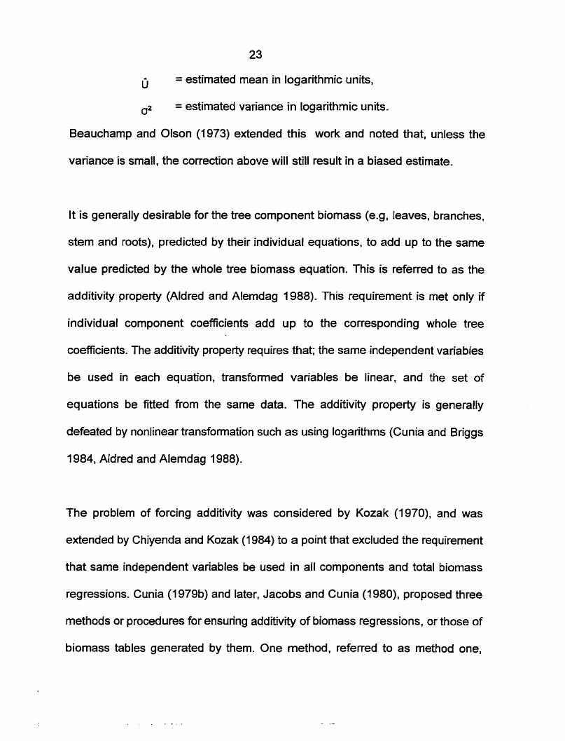
23

û = estirnated mean in logarithmic units,

u2 = estimated variance in logarithmic units.

Beauchamp and Olson (1973) extended this work and noted that. unless the

variance is small, the correction above will still result in a biased estimate.

It is generally desirable for the tree component biomass (e.g, leaves, branches.

stem and roots). predicted by their individual equations. to add up to the sarne

value predicted by the whole tree biomass equation. This is referred to as the

additivity property (Aldred and Alemdag 1988). This requirement is met only if

individual component coefficients add up to the corresponding whole tree

coefficients. The additivity property requires that; the same independent variables

be used in each equation, transformed variables be linear. and the set of

equations be fitted from the same data. The additivity property is generally

defeated by nonlinear transformation such as using logarithms (Cunia and Briggs

1984, Aldred and Alemdag 1988).

The problem of forcing additivity was considered by Kozak (1970), and was

extended by Chiyenda and Kozak (1984) to a point that excluded the requirement

that same independent variables be used in al1 components and total biomass

regressions. Cunia (1979b) and later, Jacobs and Cunia (1 980), proposed three

methods or procedures for ensuring additivity of biomass regressions. or those of

biomass tables generated by them. One method. referred to as method one,

24

requires the calculation of the regression function for each component separateiy

wÏth the regression function of the total defined and calculated as the sum of the

cornponent regressions. This method is simple and convenient to use and

achieves the desired additivity. The disadvantage is, no statement of reliability can

be made about the prediction using such a model.

The second method, designated as method two, ensures additivity by using the

same independent variables in the least squares linear regression of the biomass

of each component and that of the total. The same sets of weights must be used

if required (Cunia and Briggs 1984). The third approach uses linear regression

functions with dumrny variables. A dumrny variable is defined for each component

biomass such that, ui = 1 for cornponent I or total, and ui = O otherwise; where Y

is the dummy variable for component I. The dummy variables are used in

combination with the independent variables to generate new variables, xij = xj for

component I or total, and x, = O otherwise. The independent variables are then

combined to estimate the general equation;

Where, y is the cornponent biomass, B, is the regression coefficient of the new

predictive variable x, derived from the product of the ith dummy variable

with the jth independent variable.

25

This rnethod has the advantage of ensuring additivÏty and providing estimates for

the standard error. The disadvantage is the tedious work required, especially when

dealing with a large sample. The general equation can be estimated by ordinary

weighted least squares (OMS) or the generalized least squares (GLS)(Cunia and

Briggs 1985). Reed and Green (1985) presents an extension of this method to

cover nonlinear models.

2.5 YlELD MODELS AND TABLES

Yield tables present the anticipated yields from an even-aged stand at various

ages, and is one of the oldest approaches to yield estimation. Modem yield tables

often include not only yield, but also, stand height, diameter, number of stems,

stand basal area, and current and mean annual increments (Vanclay 1994).

Yield tables are commonly classified into normal, empirÏcal and variable-density

(Avery and BurkhaC 1994). Normal yield tables are supposed to be based on

"normaln or optimal stocking; hence, stand density is not considered. Empirical

yield tables are supposed to be based on average or actual rather than normal

stocking. Like normal yield tables, empirical yield tables are Iimited in use to the

average stocking condition upon which they are based. Variable density yield

tables include some rneasure of stand density.

26

Yield models are mathematical fundons relating yield to stand age, site index, and

some measure of stand density. The basic form of a yield model has been that

proposed by Schumacher (1939). In its simplest form. the model relates yield in

ternis of volume per hectare to stand age and site index. This model has proved

to be uçeful, reliable and widely used for many pure even-aged stands (Vanclay

1994).

MacKinney and Chaiken (1939) built upon this equation by including a measure

of stand density as an independent variable to develop what is known to be the

first variable density yield model (Clutter et al. 1983). Clutter (1963) adapted the

general form of this equation, given as;

where V is the stand volume per hectare, A is the stand age, S is the site index,

and I is some measure of stand density (usually the logarithrn of stand basal area),

to develop a compatible growth and yield model. This rnodel ensures the

compatibility of estimates of yield from tables on one hand, with figures derived

from successive surnmation of growth estimates on the other hand, based on the

same data (Vanclay 1994).

Also of common use in growth and yield modelling is the Chapman-Richards

27

growth model (Richards 1959, Chapman 1961). The model, supposedly derived

from basic biological considerations has proven to be very flexible in application

(Clutter et al. 1983). The basic form of the Chapman-Richards growth rnodel is;

(Clutter et al. 1983)

where a, p, and y are constants such that, a > O, O c p c 7 , and y > O. lntegrating

this equation gives the yield model. Vanclay (1 994) noted some doubts about the

supposed biological basis of the model, but indicated it had other merits.

Some effort has been made at modelling growth and yield using systems of

simultaneous equations (e.g, Furnival and Wilson 1971, Arnaites et al. 1984,

Borders and Bailey 1986, Borders 1989). For this approach, individual components

of growth are identified and expressed collectively as a system of equations to

predict stand growth and yield (Vanclay 1994). This system of equations are then

estimated by indirect, two-stage or three-stage least squares, or seemingly

unrelated regression techniques (Johnston 1984).

Many growth and yield models provide rather limited information about the forest

stand, but effective management and planning also require information on size

28

and the species contributing to the stand volume (Vanclay 1994). This problem is

solved by the use of diameterdistribution-based yield models.

Many probabiliity density functions can be and are used to describe stand diameter

distributions; the Gram-Charlier (Meyer 1930), beta distribution (Prodan 1953,

Clutter and Bennett 1965), Weibull distribution (Bailey and Dell 1973), gamma

distribution (Nelson 1964), Johnson's SB distribution (Hafley and Schreuder 1977),

Lognomal distribution (Bliss and Reinker 1964). For the purpose of this study, the

Weibull distribution will be discussed.

The Weibull distribution was developed by Weibull (1 95 1) to model the probability

of material failure. Bailey and Dell (1 973) are credited as the first to introduce the

Weibull distribution into forestry to model diameter distributions. The three-

parameter Weibull distribution function is defined by the probability density function

(pdf);

Where, x is a specified diameter and a, b and c are constants such that, x r O, a

O, b > 0, and c > O. The parameter a, commonly termed the location pararneter,

identifies the lower bound of the diameter distribution. For fixed values of b and c,

changes in parameter a simply shifts the entire distribution along the x-axis.

29

Parameter b is the scale parameter, and the point x=a+b corresponds

approxirnately to the 63rd percentile of the distribution (Shifiey and Lentz 1985).

Parameter c indicates the shape of the Weibull distribution. When c s 1, the

distribution has a reverse J-shape, for c > 1, the distribution is mound-shape,

approxirnating nomal distribution for c = 3.6. When c is between 1 and 3.6, the

Weibull distribution is positively skewed, and negatively skewed for c > 3.6 (Bailey

and Dell 1973). The cumulative distribution function derived as an integral of the

pdf (appendix XIV) is given by;

where, a, b and c are parameters as defined before, F(x) is the relative frequency

of a diameter class between a and x. The general expression of the above

equation is given by;

where P is the probability that a diameter is found between two lirnits L (lower limit)

and U (upper limit). For any diameter class, L and U are the lower and upper class

boundaries respectively. Therefore. by rnultiplying P by N, the number of trees in

the stand, the frequency of each diameter class is obtained.

30

There are three common rnethods of estimating the parameters of the Weibull

distribution; the maximum likelihood method (Cohen 1965, Bailey 1974, Schreuder

et ai. 1978, Gove and Fairweather 1989), the percentile method (Zankis 1979,

Clutter et al. 1983) and the method of moments (Shifley and Lentz 1985). The

maximum likelihood estimation is the rnost efficient. The moment estimators offer

speed and ease in exchange for some loss in precision. The percentile estimators

are ako easy to obtain and are even more accurate than the maximum likelihood

estimators when the shape parameter c, is less than or close to 2 (Zankis 1979).

2.6 SlTE INDEX AND SlTE QUALITY EVALUATION

For meaningful growth and yield forecasting, effective evaluation of the site

productivity is required. A lot of effort has been made in this regard to the

development of techniques for quantifying site quality. Clutter et al. (1983)

classified these methods into direct and indirect.

Direct rnethods make use of historical yield records, stand volume and height data,

which are oRen not available for most species. The indirect methods make use of

overstorey interspecies relationships, lesser vegetation characteristics, and

topographie, climatic and edaphic factors. The direct rnethods most invariably,

provide better evaluation than the indirect methods (Clutter et al. 1983).

31

Site index is the oldest indirect and the most widely used concept for evaluating

site productivity (Husch et al. 1982). Site index is conveniently defined as the total

height of specified trees in a stand at an arbitrary base age (Powers 1973). Of

common usage is the top or dominant height, defined as the average height of the

100 fattest or tallest trees per hectare. Site index curves or equations relate

dominant or top height to age. Tree height growth is used because, theoretically,

1 is sensitive to site quality differences, M e affected by varying density levels and

tree composition, relatively stable under varying thinning intensities, and strongly

correlated with volume (Avery and Burkhart 1994).

Data for the development of site index equations commonly come from three

sources; temporary plots (TSPs), PSPs or stem analysis. TSPs provide the most

inexpensive and the quickest source of data, but are based on the assumption

that, full range of site indices are well represented in al1 age classes (Alder 1980,

Clutter et ai. 1983, Avery and Burkhart 1994). This is hardly met in practice. PSPs

and stem analysis offer the most reliable data for site indices, but are relatively

slow and expensive in providing data.

Site index curves may be constructed by graphical methods or by regression

analysis. Statistically, there are three broad approaches; the guided or proportional

curve, the difference equation and the parameter prediction methods (Clutter et

al. 1983). The most frequently used equation forms are Schumacher's (1939) and

32

Chapman-Richards' (Richard 1959, Chapman 1961).

The critical silvics of teak, as well as different approaches to estimating and

modelling yie!d have been reviewed. The best option for this study, given the time

and resource constraints, was to make use of temporary plot data from plantations

of different ages since no PSP data base exists for these stands. However, the

disadvantages of this approach are generally recognized and acknowledged.

3.0 MATERIALS AND METHODS

3.1 THE STUDY AREA

The study was camed out in the Northem Region of Ghana and centered on

Tamale. Sample plantations were selected from four forest districts of the region

between May and July, 1996. These are; the Tamale, Yendi, Savelugu and

Damongo forest districts (see map in figure 1). These districts are al1 located in the

Guinea Savannah vegetation zone of the country (see figure 2).

3.1.1 The Natural Veaetation Zones of Ghana

Ghana is a tropical country with about 238,549 km2 land area. The country lies

between latitudes 4'45" and 1 Io 11" north and longitude Io 14" and 3" 07" west.

Ghana is divided into six vegetation zones as shown in figure 2.

The rainforest and the semideciduous forest zones are broadly classified as the

high forest zone. This zone occupies the southwestern third of the country and

covers an area of about 81,342 km2. The remaining 157,198 km2which constitutes

two-thirds of the country is mainiy the savannahs. These are classified as the

southem and the northem savannahs, based on the location.

10' N UPPER EAST

O 50 'Oo IM Location of Sarnple Plantations - Regional Capital

Figure 2. The study area.

35

The southem savannah type consists of the coastal scnib and grasslands

whereas the northem type is made up of the Sudan savannah and the Guinea

savannah. The Guinea savannah is by far, the largest vegetation zone of the

country (Lawson, 1968).

3.1.2 The Guinea Savannah Vegetation zone

The Guinea savannah is characterised by two distinct seasons of approximately

equal length; the wet (rainy) and the dry seasons. The dry season is characterised

by the harmattan winds, generally called the north-east trade winds. This is a very

dry ainnass, the inception of which marks the beginning of the dry season.

Characteristic of the wet season is the south Atlantic aimass, referred to as the

south-west monsoons, which are moisture laden and are known to bring about

rains. The rnean annual rainfall is between 960 mm and 1200 mm, and falls

between March and October, with the peak in July and August. The mean annual

temperature which is 28.3OC does not Vary significantly during the seasons.

The characteristic vegetation of the Guinea savannah is made up of short

deciduous, widely spaced and heavily branched fire resistant trees. They seldom

fom a closed canopy and overtop an abundance of ground flora of grasses and

shrubs of varying height (Taylor, 1952). The characteristic species are,

Buiymspenum paradoxum and Parkia clappertaniaria, found rnostly on familand.

36

Other cornmon species are, Daniellia oliveri, Burkia afkana, Terminalia spp.

The underlying geology of the zone is varied. The cornmon types however, are

the voltaian sandstone, shales and granites (Boateng, 1966). These geological

formations give rise to two broad groups of soils; the Savannah Ochrosols and the

Groundwater Laterites. The Savannah Ochrosofs are found on the voltaian

sandstones (Boateng, 1966). These consist of well drained porous loams. These

soils are among the best in the zone in spite of their deficiency in nutrients such

as phosphorous and nitrogen.

The Groundwater Laterites are the most extensive soils and are found on the

voltaian s h a h and granites. These are underlain by iron pans or mottled clay

layers, so rich in iron that it hardens to form an iron pan on exposure (Boateng,

1966). Their drainage is very poor and they tend to get waterlogged in the rainy

season and become extremely dry in the dry season. They constitute the poorest

type of soils in the zone.

3.2 DATA COLLECTION

The list of al1 teak plantations in the region was obtained from the Regionai forestry

offices and stratified into one year age classes. Plantations were sampled from

these groups with an effort to equal allocation of three sample plantations to each

Figure 2. Natural vegetation zones of Ghana (Source: Traced from the Atlas for Ghana p12)

'l'ropical R a h Forest Coastal Scnib &

Grassland

38

age group, except for those ages in which the number of plantations was less than

three. For each age group, an effort was also made to cover the full range of site

conditions (from the poorest to the best). A pre-sample inspection was done to

assess the conditions of each plantation considered for sampling . Plantations that

were found to be badly understocked due to mortality or harvesting were discarded

and replaced.

In al1 25 plantations were sampled, ranging in age from 3 to 40 years, with a total

of 100 temporary sample plots. For each sample plantation, the following

operations and rneasurements were carried out;

a) Four circular plots each of radius 7 rn (approximately, 0.01 5 ha) were selected

at random. Circular plots were used to avoid directional bias.

b) For each plot, al1 teak trees enclosed were measured for diameter at breast

height (dbh) (in centimeters), total height (in rneters) and numbered to facilitate

relocation. For trees forking below breast height, the diameter of each leader was

measured separately and their quadratic mean calculated; the height of the tallest

leader was recorded to correspond with the quadratic mean diameter.

c) With the help of a random number generator, three (3) trees were selected at

random from each plot as sub-sample trees and felled for detailed measurements.

39

The srnall sub-sample size was a compromise between data adequacy and

destruction of tree value.

d) For each sub-sample tree;

i) Detaiied measurernents were taken for diameter at the base or sturnp level (DA),

breast height (dbh), at half the height above breast height (D3), at the top 1 cm

(D4) and the total height of the main stem.

ii) All leaves and branches were separated from the bole and weighed and sub-

sarnples taken for oven dry weight detemination;

iii) The main stem was weighed and sub-samples taken for oven dry weight

determination. Samples were taken at strategic positions to minimize error due to

the variation in moisture content along the stem;

iv) The sub-samples of parts taken in ii) and iii) above were clearly labelled by tree

number, plot, and plantation location, and dried in an oven at a temperature of

about 70°C to constant weig ht.

For trees that were too large to be weighed directly in the field, cross-sectional

discs were taken from the base and the top sections of the bole and each

40

weighed. The volume measurements of each disc were taken and by simple

proportions, the fresh weight of the whole bole was detennined. The equipment

used in weighing fresh biomass was a load cell suspended from a tree with a

motorcycle battery as the source of power. Small samples (sub-samples) were

weig hed using an electronic scale.

Growth and yield survey data for teak plantations in the high forest zone of Ghana

were obtained from the Ghana Forestry Department Planning Branch, Kumasi,

Ghana for cornparison. A summary of part of this data is presented in appendix IX.

The ages of these plantations ranged from 13 to 26 years and were al1 from the

Offinso Forest District of the Ashanti Region.

3.3 DATA ANALYSE

3.3.1 Volume Estimations

The volume of each sub-sample tree was computed using Smalian's formula. The

stand volume was estimated by three different methods and compared:

a] As two-stage simple random sampling, the estimated total volume per hectare

and the corresponding variance was calculated from (Cochran 1 977) as;

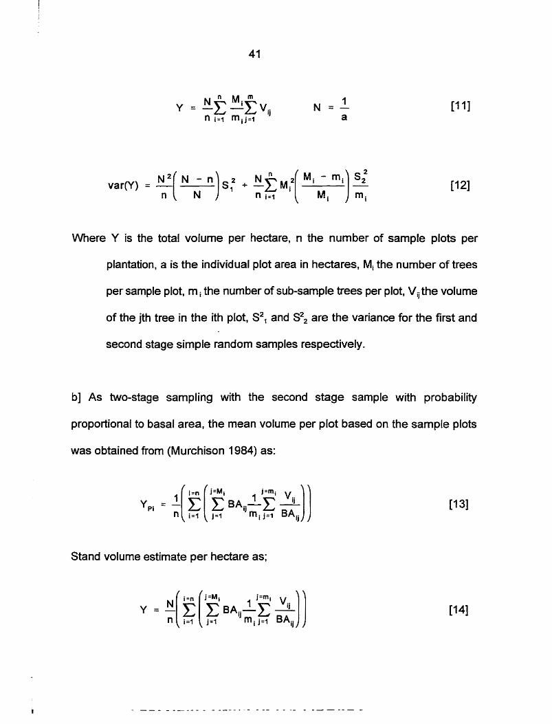
Where Y is the total volume per hectare, n the number of sample plots per

plantation, a is the individual plot area in hectares. Mi the number of trees

per sample plot, m the number of sub-sample trees per plot, Vii the volume

of the jth tree in the ith plot, S2, and S2, are the variance for the first and

second stage simple random samples respectively.

b] As two-stage sampling with the second stage sample with probability

proportional to basal area, the mean volume per plot based on the sample plots

was obtained from (Murchison 1984) as:

Stand volume estirnate per hectare as;

42

where, V,, Mi. mi, Y. N and n are as defined before and BA ,is the basal area of the

jth tree from the I h sample plot and YPi, is the total volume of the ith plot. The

variance was calculated using the formula from Murchison (1984, page 63), given

as;

Where S2, and SZ2 are the first and second stage sample variances, given as;

It should be noted that, S2, is a measure of the variation between individual sub-

sample tree estimates of plot totals; not the variation between individual sub-

sample tree volumes (Murchison 1984).

c] A standard volume equation was constructed using the individual tree dbh,

height and volume measurements. The fifteen most commonly used equations

presented in Unnikrihnan and Singh (1 984) were each tested. The rnodel that

43

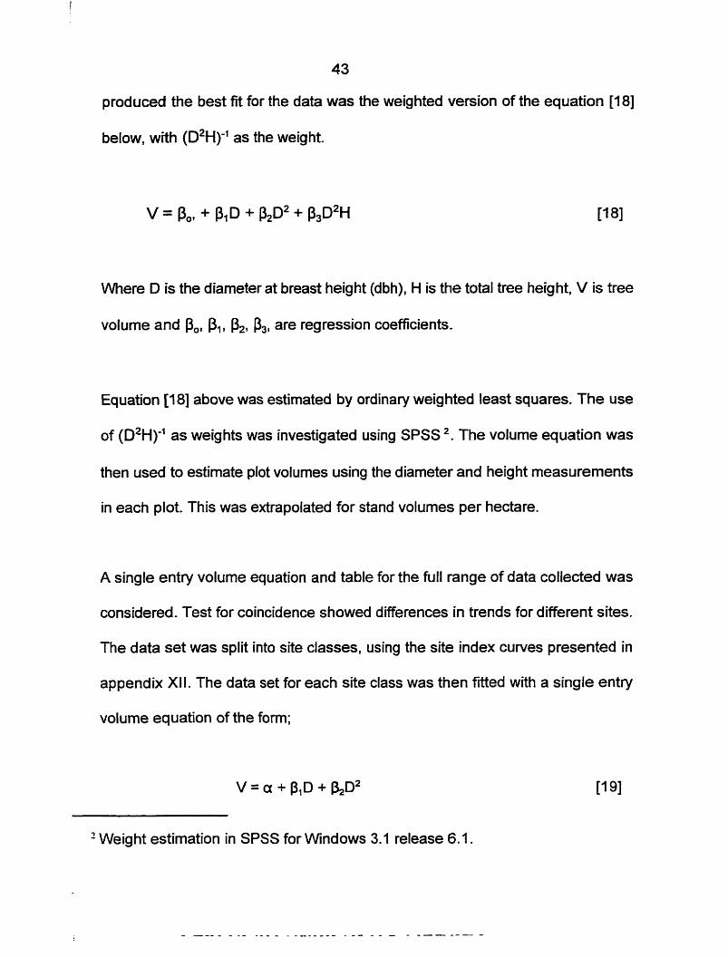
produced the best fit for the data was the weighted version of the equation [18]

below, with (D2H)-' as the weight.

Where D is the diameter at breast height (dbh), H is the total tree height, V is tree

volume and p,, Pl, P,, P3, are regression coefficients.

Equation [18] above was estimated by ordinary weighted least squares. The use

of (D2H)-' as weights was investigated using SPSS 2. The volume equation was

then used to estimate plot volumes using the diameter and height measurements

in each plot. This was extrapolated for stand volumes per hectare.

A single entry volume equation and table for the full range of data collected was

considered. Test for coincidence showed differences in trends for different sites.

The data set was split into site classes, using the site index curves presented in

appendix XII. The data set for each site class was then fitted with a single entry

volume equation of the fom;

Weight estimation in SPSS for Windows 3.1 release 6.1.

44

Heteroscedasticity was corrected for each equation by weighting. The appropriate

weighting variable was determined as a function of dbh, D using SPSS. The

variable D4 produced well behaved residuals and was thus used as weights for

each site class.

Biomass Computations

The oven dry weight of each component of the sub-sample trees was determined

by simple proportions from the weights of theoven dry sarnples. These were

summed up to give the above ground biomass of each tree. Based on the sample

tree dry weig hts, biomass equations were developed for the construction of

biornass tables. To ensure additivity, the dummy variable rnethod (Jacobs and

Cunia 1980. Cunia and Briggs 1984) was used to estimate the biomass equations

by weighed least squares (VVLS). Dummy variables Ui were defined such that; Ui

= 1 for component I and total tree biomass, and Ui = O otherwise. The components

of biomass were leaves, branches and stem. For instance. if the leafy component

biomass is considered. its dummy variable took the value 1 for leaves and total

biomass, and O othennrise.

Prior to estimating the general equation, the equation of each component was

estimated to determine the regression standard errors for each component. The

standard error for the individual cornponents were used in combination with the

45

transformation vector (D)' as weights.

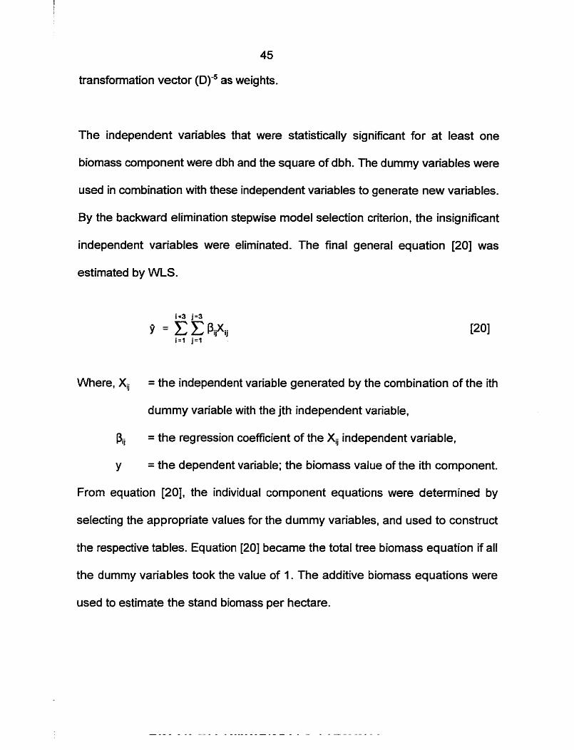
The independent variables that were statistically significant for at least one

biomass component were dbh and the square of dbh. The dummy variables were

used in combination wlh these independent variables to generate new variables.

By the backward elimination stepwise model selection criterion, the insignificant

independent variables were eliminated. The final general equation [20] was

estimated by WLS.

Where, Xij = the independent variable generated by the combination of the ith

dummy variable with the jth independent variable,

pi, = the regression coefficient of the Xi independent variable,

Y = the dependent variable; the biomass value of the ith component.

From equation [20], the individual component equations were determined by

selecting the appropriate values for the dummy variables, and used to construct

the respective tables. Equation [20] became the total tree biomass equation if al1

the dummy variables took the value of 1. The additive biomass equations were

used to estimate the stand biomass per hectare.

3.3.3 Yield Models

Plots were classified using the proportional curves method described by Alder

(1 980). A single equation was fitted to the plot level top heighr - age data, using

the logarithmic transformation of Schumacher's (1 939) equation:

Where T, is the mean top height, T,, is the maximum height the species could

reach on the site, A is the age of the stand, p is regression coefficient and

k is a constant.

By nonlinear regression, the value of k was detenined iteratively for the value that

minimized the sum of squared errors. The value of k was found to be %. This was

used to transform the age variable and by ordinary least squares, the equation;

was estirnateci. Site classes were determined by allowing the regression constant

(which in this case is In TmJ to Vary to produce curves with the sarne gradient and

The average height of the largest 100 trees per hectare.

47

different intercepts (anamorphic curves). This method has been recornmended for

use when only temporary sample plot data such as in this study, are available

(Alder 1980).

Based on the site index curves estimated above, plantations were sorted

according to site classes, and fitted wlh a general yield equation of the form;

Where Q is sorne rneasure of yield (mean dbh, mean Height, stand volume per

hectare, basal area or biomass per hectare), A is plot age, S is the site

index, I is some measure of stand density and Bo R , P,, B, , and k are

constants.

The value of k equal to % was used. Basal area was used as a measure for stand

density for the volume yield equation, but was found to be statistically insignificant

and was dropped from the model. Thus equation [23] was reduced to equation [24]

for each site class.

This was estimated as the yield equation for each measure of yield for each site

48

class. The volume yield model was divided by age to obtain the model for mean

annual volume increment (MAI) (equation [25]). The current annual increment

(CAI) rnodel was obtained by taking the derivative of the volume yield mode1 with

respect to age (equation [26]). The ages of maximum MAI and CA1 respectively

were detemined by taking the derivatives of each of equations [25] and [26],

setting them to zero and solving for A.

MAI = Q/A = (A-') EXP (a + PAX)

Asyrnptotic height - dbh relationship was estimated for the different site classes,

using the Chaprnan-Richards function (Richards 1959). The asymptotic rnodel was

considered because, by it's mathematical fom, it offers flexibiliity for extrapolations

beyond the ernpirical data set (Ganan et al. 1995). Estimation of the equation

parameters was done by nonlinear regression using SPSS. The equation as

presented by Gannan et al. (1 995) is given as:

where, H is the total height. Po, P,, P, are regression constants, Pois the asymptotic

height. A regression equation was generated for each site class.

49

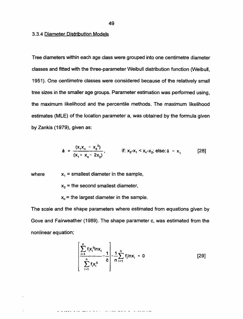
3.3.4 Diameter Distribution Models

Tree diameters within each age class were grouped into one centirnetre diameter

classes and fitted with the three-parameter Weibull distribution function (Weibull.

1951). One centimetre classes were considered because of the relatively small

tree sizes in the smaller age groups. Parameter estimation was performed using,

the maximum likelihood and the percentile methods. The maximum likelihood

estirnates (MLE) of the location parameter a. was obtained by the formula given

by Zankis (1 979), given as:

if: x,-X, < xn-x2; else: â = x, [28]

where x, = smallest diarneter in the sample,

x, = the second smallest diameter,

x,, = the largest diameter in the sample.

The scale and the shape parameters where estimated from equations given by

Gove and Fairweather (1989). The shape parameter c, was estimated from the

nonlinear equation;

50

iteratively, and substituted into the equation;

6 =

for the estirnate of b;

Where, fi is the ith diameter class frequency and x i is the corresponding class

midpoint. The parameter estimates obtained by this method were cross checked

by estimating the three parameter Weibull function iteratively by nonlinear

regression (SPSS).

The percentile estimates (PE) of the parameters were obtained using the

equations proposed by Zankis (1 979). The parameter a was estirnated by equation

[28] above. The pararneters c and b were estimated from:

and

respectively.

Where, pi = 0.16731, p, = 0.97366 and 0.63n = 63rd percentile in the sarnple and

n is sample size.

Goodness of fit was tested by using the KolrnogorovSmimov (KS) criterion (Daniel

1978). This criterion utilizes the maximum absolute differences between the

cumulative observed and predicted diameter probabilities to determine goodness

of fit. These differences are compared with statistics (KS statistics) given in tables

at various probability levels. A hypothesis is rejected if the maximum absolute

difference exceeds the tabulated KS-statistic at the chosen probability level and

sarnple size.

52

4.0 RESULTS

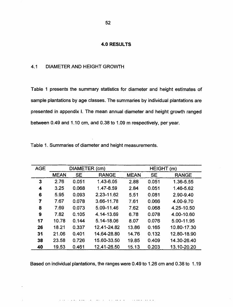
4.1 DIAMETER AND HEIGHT GROVVTH

Table 1 presents the summary statistics for diameter and height estimates of

sample plantations by age classes. The summaries by individual plantations are

presented in appendix i. The mean annual diameter and height growth ranged

between 0.49 and 1 . I O cm, and 0.38 to 1 .O9 m respectively, per year.

Table 1. Summaries of diameter and height measurernents.

AGE DIAMETER (cm) HEIGHT (ml MEAN SE RANGE MEAN SE RANGE

3 2.76 0.051 1.43-6.05 2.88 0.051 1.36-5-55 4 3.25 0.068 1 -47-8.59 2.84 0.051 1.46-5.62 6 5.95 0.093 2.23-1 1.62 5.51 0.081 2.90-9.40 7 7.67 0.078 3.66-1 1.78 7.61 0.066 4-00-9.70 8 7.69 0,073 5.09-1 1.46 7.62 0.068 4.25-1 0.50 9 7.82 0.105 4.14-1 3.69 6.78 0.078 4.00-1 0.60 17 10.78 0.144 5. 1 4-1 8.06 8.07 0.076 5.00-1 1.95 26 18.21 0.337 12.41-24.82 13.86 0.165 10.80-1 7.30 31 21 .O6 0.401 14.64-28.80 14.76 0.1 32 12.80-A 8.90 38 23.58 0.726 15.60-33.50 A9.85 0.409 14.30-26.40 40 19.53 0.461 12.41-26.50 15.13 0.203 13.4'0-20.20

Based on individual plantations, the ranges were 0.49 to 1.26 cm and 0.38 to 1.19

53

m respectively. The mean annual diameter growth recorded for teak plantations

in the high forest zone of Ghana ranged from 1.1 to about 2.0 cm per year

(appendix IX).

Table 2. The estimates of the Weibull parameters by the Maximum likelihood (MLE) and the Percentiles (PE) methods

- - -- - - - - - - - -

AGE MAXIMUM LIKELIHOOD PERCENTILE ESTIMATE C/RS) ESTIMATES

The parameter estimates of the Weibull distribution for teak in Northem Ghana and

the coefficients of the asymptotic heightdbh function are presented in tables 2 and

3 respectively. The surnmaries of observed and predicted diameter frequencies

by the h o parameter estimation methods are presented in appendix XI. Ten out

54

of the eleven hypotheses tested were acceptable for the maximum likelihood

estimates and eight out of the 11 for the percentile estimates at 0.05 probability

level. This is generally an indication of good fit. As indicated by the estimates of

the parameter c, the general shape of the diameter distribution curve is mound-

shaped, and since none of the estirnates exceeds 3.6, the distributions are

positively skewed.

In Table 3, the regression constants Bol represent the maximum total heights on

the sites, pl is a measure of steepness of the cuve and p,is curvature parameter.

As shown in Table 3, if teak is allowed to grow for a long period of time, the

estimated maximum (asyrnptotic) height is 32.84 m on site class 1, 22.50 m on site

class II and 15.91 on site cfass III.

Table 3. Coefficients and standard errors of height - dbh equation.

SITE CLASS ESTIMATES OF COEFFICIENTS

55

4.2 VOLUME ESTIMATION

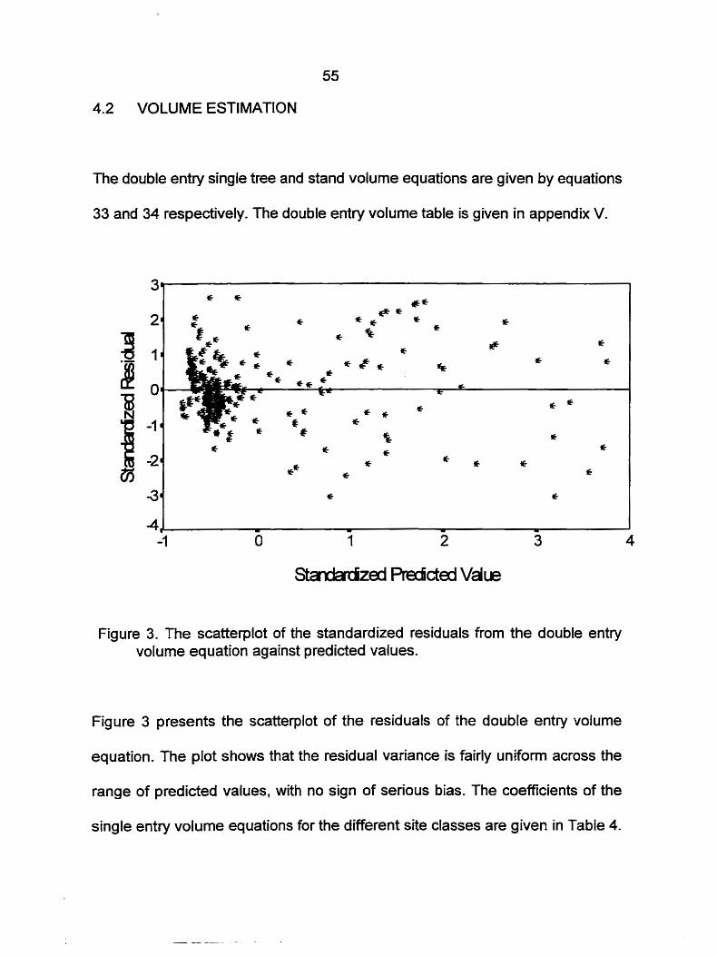
The double entry single tree and stand volume equations are given by equations

33 and 34 respectively. The double entry volume table is given in appendix V.

Figure 3. The scatterplot of the standardized residuals from the double entry volume equation against predicted values.

Figure 3 presents the scatterplot of the residuals of the double entry volume

equation. The plot shows that the residual variance is fairly uniform across the

range of predicted values. with no sign of serious bias. The coefficients of the

single entry volume equations for the different site classes are given in Table 4.

56

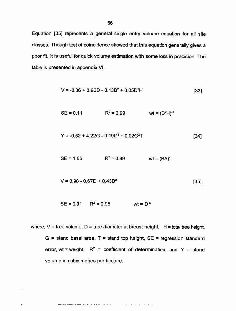
Equation [35] repfesents a general single entry volume equation for al1 site

classes. Though test of coincidence showed that this equation generally gives a

poor fit, it is useful for quick volume estimation with some loss in precision. The

table is presented in appendk VI.

where, V = tree volume, D = tree diameter at breast height, H =total tree height,

G = stand basal area, T = stand top height, SE = regression standard

error, wt = weight, R2 = coefficient of determination, and Y = stand

volume in cubic metres per hectare.

Table 4. Coefficients of local volume equations by site classes.

SITE CLASS COEFFICIENTS

CONSTANT

The summaries of the artificial and absolute cylindrkal form factors, and the

absolute fom quotients are presented in Table 5. The absolute fotm factors are

based on the diameter at the stump level whereas the artificial form factors are

based on diameters at breast height. The absolute fom factors indicates that, tree

volumes tend to be higher than, but closer to those of cones, than they are to

cylinders, of the sarne basal areas. The artificial form factors range from 0.62 to

1.59.

The absolute form quotients are fairly stable and Vary from 0.57 to 0.77. This is the

ratio of the diameter at half the height above breast height to the dbh. The values

show that, there is in general, a 23 to 43% decrease in diameter from breast

height to the point half the height above breast height.

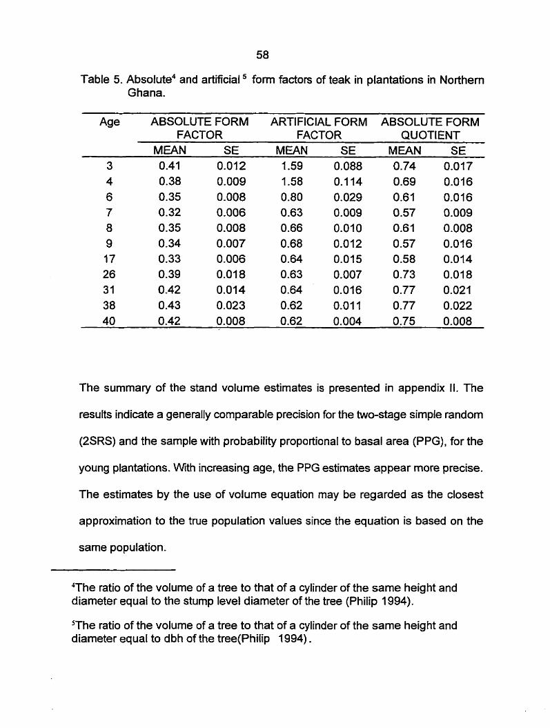
Table 5. Absolute4 and artificial form factors of teak in plantations in Northem Ghana.

Age ABSOLUTE FORM ARTIFlClAL FORM ABSOLUTE FORM FACTOR FACTOR QUOTIENT

The summary of the stand volume estimates is presented in appendix II. The

results indicate a generally comparable precision for the two-stage simple random

(PSRS) and the sample with probability proportional to basal area (PPG), for the

young plantations. Wth increasing age, the PPG estimates appear more precise.

The estimates by the use of volume equation may be regarded as the closest

approximation to the true population values since the equation is based on the

same population.

4The ratio of the volume of a tree to that of a cylinder of the same height and diameter equal to the stump level diameter of the tree (Philip 1994).

5The ratio of the volume of a tree to that of a cylinder of the same height and diameter equal to dbh of the tree(Philip 1994) .

59

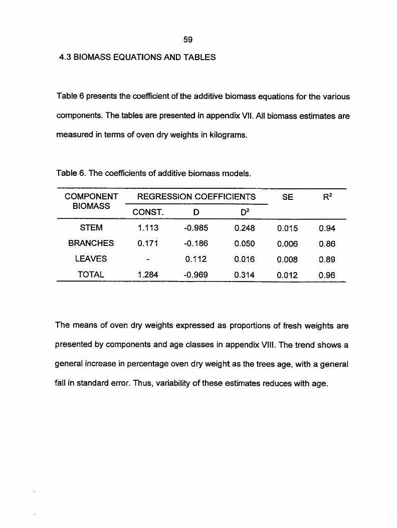
4.3 BIOMASS EQUATIONS AND TABLES

Table 6 presents the coefficient of the additive biomass equations for the various

cornponents. The tables are presented in appendix VII. All biomass estimates are

measured in ternis of oven dry weights in kilograms.

Table 6, The coefficients of additive biomass models.

COMPONENT REGRESSION COEFFICIENTS SE R2

STEM 7.113 -0.985 0.248 0.01 5 0.94

BWNCHES 0.171 -0.186 0.050 0.006 0.86

LEAVES - 0.1 12 0.016 0.008 0.89

TOTAL 1 284 -0.969 0.314 0.012 0.96

The means of oven dry weights expressed as proportions of fresh weights are

presented by components and age classes in appendix VIII. The trend shows a

general increase in percentage oven dry weight as the trees age, with a general

fall in standard error. Thus, variability of these estimates reduces with age.

60

4.4 YIELD MODELS AND TABLES,

Table 7. Regression coefficients for component yield models for plantation teak in northem Ghana from equation [25].

--

YIELD SITE CLASS I SITE CLASS II SITE CLASS III VARIABLE

a P SE a P SE cx B SE

MEAN dbh 4.20 -4.88 0.07 3.94 -5.50 0.09 3.58 -6.20 0.06

BASAL 6.10 -9.20 0.17 5.73 -10.73 0.19 4.95 -1j.75 0.18 AREA

VOLUME 8.10 -11.13 0 1 7.87 -12.33 0.12 7.20 -14.12 0.13

BIOMASS 7.69 -10.68 0.20 7.19 -12.23 0.19 6.62 -12.85 0.19

The regression coefficients of the yield models are given in table 7. The yield table

is presented in appendix X. The mean and current annual incrernent are estimated

to peak at ages; 14 and 31, 17 and 38. and 21 and 48 respectively for Site classes

1, II and III (see appendix X).

The site index curves are presented in appendix XII. The site index equation is;

61

where T is the top height of the plantation, S is the site index of the plantation at

the base age 20 years and A is the stand age.

A plot of the average top heights predicted for site class I in the study area with

figures from the lndian yield tables for site class III (Laurie and Ram 1940) and

Trinidad site class II (Miller 1969) are given in Figure 4. The three curves generally

show a simitar trend.

5.0 DISCUSSION

5.1 ASSESSMENT OF GROWH AND YlELD OF TEAK IN NORTHERN GHANA

The major limitation of this study was time and budget constraints which resulted

in a small data size. This is a general disadvantage of the use of temporary

sample plots in yield modeliing. Besides. there was poor representation of the

older age classes in the sarnple. This was a result of the general lack of

plantations within these age classes. Thus, it is possible that, the average growth

trend might not have been adequately defined.

Also of notable limitation is the sub-sample size, which was small. This was due

to concerns about the value of teak and the amount of destruction that rnay be

associated with large sub-sarnples. The bias that might result from the small sub-

sample size rnay be minimized by the relatively uniforni growth conditions reflected

in the small standard errors observed in appendix 1. Also, sub-samples were

selected at random, which should result in unbiased data.

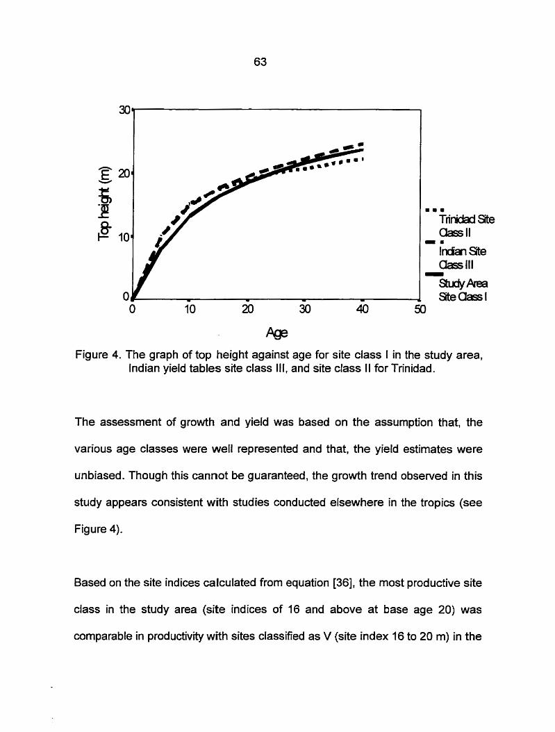
m..

Tririictad Site aass II

- 8

Indian Site aass III

œ

Shdy- SeUass I

Figure 4. The graph of top height against age for site class l in the study area, Indian yield tables site class III. and site class II for Trinidad.

The assessrnent of growth and yield was based on the assumption that, the

various age classes were well represented and that, the yield estimates were

unbiased. Though this cannot be guaranteed. the growth trend observed in this

study appears consistent with studies conducted elsewhere in the tropics (see

Figure 4).

Based on the site indices calculated from equation (361, the most productive site

class in the study area (site indices of 16 and above at base age 20) was

comparable in productivty with sites classified as V (site index 16 to 20 m) in the

64

high forest zone of Ghana (appendix IX). This is not surprising because soils and

climatic conditions in this zone compare much more favourably with average

requirements for the growth of teak than the conditions in the study area. This site

class was also comparable in productivity to site class III in the Indian yield tables

(Laurie and Ram 1940) and to site class II for Trinidad (Miller 1969) (see figure 4).

Thus, if the site indices tnily reflect the productive potential for teak in Northern

Ghana, then the potential for teak in the region is considerable.

An examination of the stocking levels indicates that, plantations in the high forest

zone rarely exceeded 400 stems per hectare. The spacing factors, calculated by

expressing average plant spacing as a percentage of average top height, were

generally between 30 and 40%, as compared to 15 and 20 observed in the study

area for plantations with ages above 17 years. Though the former may represent

slight understocking, it is outside the scope of this study to comment. The

projected mean diameters from the yield table in appendix X at age 40, based on

these growth conditions are, 30.83, 21.55 and 13.46 for site classes I l II, and III

respectively. The corresponding yields on per hectare basis are, 566.91, 372.58

and 143.66 m3 respectively. Though these yields look encouraging, the generally

srnaIl mean diameters indicate that, most of the yield will be trees of smaller sizes.

This is supported by the positive skewness in diameter distribution. This indicates

the lack of and the need for thinning in such plantations.

65

The spacing factors of the very young plantations were very high (above 50%).

This is partly attributed to the time it takes for the species to fully "capture" a site,

due to the relatively low growth rates, and partly due to initial mortality. Mortality

is mainly caused by unfavourable climatic conditions such as lack of rains during

the time of planting. Initial mortality creates gaps, which tend to defeat the

"trainingn of the species in the early stage of the growth, resulting in poor forms.

This is a probable explanation for the generally low absolute form factors

observed, with trees boles tending to be more conical than cylindrical.

It is clear from this assessrnent that, teak has a potential on good sites in the study

area. Considerable improvements in the quality and volume of yield can be

achieved by adopting appropriate management pracüces such as thinning, which

is not done currently.

5.2 STAND VOLUME ESTIMATION

The double entry volume equation presented in this study has been shown to be

unbias. The sarnple size was also large enough (about 289 trees) to adequately

define the volume equations. There is the need for testing of this equation with an

independent set of data to establish the presence of and the nature of any

prediction bias for appropriate correction. It is generally dangerous to extrapolate

for volume rneasurements outside the range of data used in constructing the

volume tables and this is not recomrnended.

The major limitation of the stand volume equation is that. if plantation management

regimes dRer from what is observed in this study, esthates may not be accurate.

Besides, estimates of the input variables are seldom available and will have to be

derived or based on expected optimums. The error in yield estimates will thus

corne from two sources; sampling and measurernent errors in estimating input

variables and error in estimating volume using the equation. This error could be

quite large, affecting the accuracy and reliability of the yield estimates.

The general single entry equation (equation 33) can be used if only rough

estimates are desired, with some loss in accuracy. A casual examinaüon of the

coefficients of these equations (Table 4) shows that, the coefficients for site

classes I and III are close to those of the general model, with those of site class

II appearing much different The general local volume equation may produce good

results for site classes I and III, though no effort was made to investigate this.

When estimates of higher precision are desired, it is recommended that, the

double entry volume equation be used. Diameter and height data are fed into the

model to generate the individual tree volumes. These are then summed to produce

an estirnate for the stand.

67

Using two-stage sampling with probability proportional to basal area at the second

stage (PPG) has been shown to result in improved precision over the rnean tree

method (two-stage simple random sampling). The sub-sample size of three

appeared not to be adequate for the mean tree method especially for the higher

age classes. Apparently, these findings are consistent with those of Murchison

(1990). who found out that, a sub-sample size of 3 to 6 trees per plot was

adequate for the PPG but not for the mean tree method. If absolutely necessary,

the PPG method should be given preference over the mean tree method. The use

of the volume equations is recommended if a compromise is sought between data

adequacy and tree value, limiting the sub-sample size to figures less than or equal

to three.

5.3 BIOMASS EQUATIONS AND TABLES.

The biomass rnodels were developed to ensure additivity. This may be useful for

future studies and research which may require this property. However, for

quantifying products for valuation purposes, this property may not be important.

The method chosen to ensure additivity provides estimates for the standard error

for the total above ground biomass model. This allows for the statement of

reliability to be made. One disadvantage with this method is that, the component

biomass models may not be individually, the best models in ternis of meeting the

68

regression assumptions. Presumably. by using the individual cornponent standard

errors as weights the component additive models should approach their

individually best models.

5.4 YlELD MODELS AND TABLES.

The yield rnodels and tables presented in this study are empirical as they

represent average conditions of stocking only. No consideration is given to stand

density. Plantations included in this study have a history of 2 by 2 rn planting

spacing. No thinning has been done in these plantations and missing trees are

assumed to be the result of natural mortality. Though some random tree cuttings

were observed in some plantations. basal area as a rneasure of stand density was

statistically insignificant in estimating the volume yield model. This rnay be an

indication that these random cuttings did not significantly influence yield estimates.

The mean annual volume increments are estimated to peak at the ages; 31, 38

and 48 respectively for site classes 1, ll and III. These may represent the

biologically optimum rotation ages for teak on the various site classes in Northern

Ghana. At these ages, it may be possible to obtain some trees of timber size and

for electric transmission poles on site classes I and II. The estimated mean annuai

increments at these ages are; 14.40, 9.32 and 4.05 m3 per hectare per year.

69

Yield can be estimated using either the tables or the equations presented in table

7. To estimate yield, there is the need to know the plantation age. Wth the site

class detemined using the site index curves presented in appendix XII, the

appropriate yield table is chosen. The volume yield estirnate is obtained by taking

the product of the stocking factor and the volume yield presented in the tables.

Care rnust be taken when using the tables, not to extrapolate beyond the range

of the data used in the study as this may result in serious bias. The nature of this

bias is not known at present. Bias may be due to under representation of

plantations in the older age classes. The danger is that, if the older plantations

included in the study were generally located on good sites, the tables will tend to

over-estimate yields in those age classes. The reverse is true if they were found

on poor sites. Though ocular observation of the plantation during sampling did not

reveal any of the above, this danger cannot be ruled out.

There is the need for permanent or semi-permanent plots to validate and to

determine the nature of the bias that may be associated with the use of these

tables. Until this is done, these tables remain provisional.

The site index curves were also based on the assumption that, al1 site conditions

have equal likelihood of being represented in each age class. Though a conscious

effort was made to include al1 sites in each age class, sorne age classes were

70

lacking. This assurnption cannot therefore be guaranteed. The curves in Figure 4

however show consistency of results of this study with those of other studies.

Thus, the site index curves presented here can be considered useful until curves

based on larger data sets are available. The functions presented here need

validation with broader data sets. The curves will be useful for classifying sites in

Mure studies, especially when permanent plots are to be established to represent

al1 site classes.

5.5 DIAMETER DISTRIBUTION MODELS

The results of the study show that, the three-parameter Weibull distribution model

is adequate for fitting diameter distribution of teak in Northern Ghana, under the

current management regimes. The maximum likelihood method was superior to

the percentile method in estimating the parameters.

For the younger plantations, the percentile estimates were equally as good in fit

as the maximum likelihood estimates. Zankis (1979) has indicated the percentile

estimators are simple and more accu rate than the maximum likeli hood estimators

when c, the shape parameter is less than 2 and the sample size is small. Zamoch

and Dell(1985) have also shown that the percentile estirnators were comparable

to or even better than the maximum likelihood estirnators when c is close to or less

than 2; but inferior for most forestry applications where c is generally greater than

71

2. For positively skewed distributions a s observed for this study, the predictive

abilïty of the percentile estimators will generally be good.

Zarnoch and Dell (1985) have also demonstrated the insensitivity of the Weibull

function to variation in parameter estimates. Their results showed that though the

parameter estimates may be considerably inaccurate, the resulting percentile

estimates are generally accurate. Therefore, though the percentile estimates rnay

not be precise, their frequency prediction can be expected to be good.

6.0 CONCLUSIONS AND RECOMMENDATIONS

Teak plantations in the study area are generally less productive than plantations

in the high forest zone of Ghana. The most productive sites in the study area are

comparable only to sites classified as class V in the high forest zone in terms of

productivity. The potential of teak on such sites is considerable.

Teak can be grown on an estimated biologically optimum rotations of 31, 38 and

48 years on site classes 1, II and II1 respectively. However, if timber quality is

desired, this period may have to be extended. Maximum current annual

increments are estimated to occur at 14, 17 and 21 years respectively.

Site indices of 19, 14 and 10, at the base age of 20 years, are estirnated for teak

in Northern Ghana, to correspond with site classes 1. II, and III respectively.

The three parameter Weibull probability densty function is adequate for describing

diameter distributions of teak plantations in Northern Ghana. The maximum

likelihood and the percentile methods can be used for parameter estimation.

The site index curves and yield models are provisional and rnust be regarded as

such. There is the need for validating these in further studies, with data from

73

permanent or semi-permanent growth plots.

It is recommended that the current planting spacing of 2 by 2 rn be reduced to

about 1.8 by 1.8 m to accommodate initial mortality. Othewise, "beating upn

should be encouraged to maintain optimum stocking levels. Thinning and other

management practices should be considered sen'ously especially for plantations

on good soifs.

The sub-sample size of three trees per plot was admittedly, too small for

estimating stand volume by the WC-stage simple random sampling method. It is

recommended that, in future studies, the sample size be increased if possible;

othewise the use of the volume tables developed in this study be considered.

Adegbeihn, J. 0. 1982. Preliminary results of the effects of spacing on the growth and yield of Tectona grandis, Linn F. lndian forester 108(6): 423-430.

Akindele, S. 0. 1991. Developrnent of site index equations for teak plantation in Southwestern Nigeria. J. of Trop. For. Science. 4: 162-1 69.

Alder, D. 1980. Forest volume estimation and yield prediction, Vol 2 : Yield prediction. FA0 forestry paper 22. Rome. 194pp.

Alder, D and T. C. Synott. 1992. Permanent sample plot techniques for mixed tropical forests. Tropical forestry paper No. 25. Oxford Forestry Institute. 124pp.

Aldred, A.H. and 1. S. Alemdag. 1988. Guidelines for forest biomass inventory. Canadian Forestry Serv. Info. Rep. PI-X-77. Petawa National Forestry Institute. 134pp.

Amaites, R. L.,Burkhart, H. E., Greber, B. J-, and E. E. Watson. 1984. A cornparison of approaches for predicting multiple product yields from weight scaling data. For. Sci. 3O:WI -998.

Anon. 1992. Summary of survey data for teak. Ghana forestry Department records, Planning Branch, Kumasi, Ghana (Unpub.).

Applegate, G. B., Gilmore, D. A. and B. Mohns. 1988. The use of biomass estimation in the management of forests for fuelwood and fodder production. Comrnonw. For. Rev. 67: 141-147.

Avery, T. E. and H. E. Burkhart. 1994. Forest measurements. 4th ed. McGraw-Hill Book Co. New York. 408pp.

Bailey, R. L. 1974. Announcement: computer programs for quantifying diameter distribution with Weibull function. For. Sci. 20229.

Bailey, R. L. and T. R. Dell. 1973. Quantifying diarneter distribution with the Weibull function. For. Sci. 19: 97-1 04.

Baskerville, C. L. 1965. Estimation of dry weight of tree components and total standing crop in confer stands. Ecology 46: 867-869.

Baskerville. G. L. 1972. Use of logarithmic regressions in the estimation of plant biomass. Can. J. For. Res. 2: 49-53.

Beauchamp, J. J. and J. S. Oison. 1973. Correction for bias in regression estimates after logarithrnic transformation. Ecology 54: 1402-1407.

Bickford, A. C. 1956. Proposed design for continuous inventory: A system of perpetual forest survey for the North US Forest Service Eastern Techniques meeting, Forest survey, Cumberland Falls, K. Y. October 8-1 3, 1956.

Bliss C. L. and K. A Reinker, 1964. Lognormal approach to diarneter distributions in even-aged stands. For. Sci. 10: 350-360.

Boateng, E. A. 1966. A geography of Ghana. 2nd ed. Cambridge Univ. press. 212pp.

Borders, B. E. 1989. A system of equation in forest modelling. For. Sci. 35: 548- 556,

Borders, B. E. and R. L. Bailey. 1986. Compatible systems of growth and yield equations of slash pine fitted with restricted three-stage least squares. For. Sci. 32: 185-201.

Borota, J. 1991. Tropical forests: Sorne Afncan and Asian studies of composition and structure. Elsevier. New York. 274pp.

Briscoe, C. B. And R. Ybarra-Conorodo. 1971. lncreasing the growth of established teak. Res. Notes. ITF-13, Rio Piedras, PR. USDA For. Serv. Inst. of tropical forestry. 6pp.

Brownlee, K. A. 1967. Statistical theory and methodology in science and engineering. 2nd ed. John Wiley and Sons. New York. 400pp.

Bruce, D. and L. H. Reineke. 1931. Correction alignment charts in forest research. USDA Tech. Bu!. 21 0 . 8 7 ~ ~ .

Chapman, D. G. 1961. Statistical problems in dynamics of exploited fisheries population. In Proc. 4th Berkeley Syp. Math. Sat. and Prob. Univ. Calif. Press, Berkeley, pp 1 53-1 68.

Chapman, H. H. and W. H. Meyer. 1949. Forest mensuration. McGraw-Hills Co. New York. 522pp.

Chiyenda, S. S. and A. Kozak. 19û4. Additivity of component biornass regression equations when the underlying model is linear. Can. J. For. Res 14: 441- 446.

Clutter, J. L. 1963. Compatible growth and yield models for loblolly pine . For. Sci. 9: 354-376.

Clutter J. L. and F. A. Bennett. 1965. Diameter distribution in old field slash pine plantations. Georgia For. Res. Council Rep. 13, 9pp.

Clutter, J. L.; Fortson, J. C.; Pienaar, 1. V.; Brister. G. H. and R. L. Bailey. 1983. Timber management - a quantitative approach. John Wiley and Sons, New York. 333pp.

Cochran, W. G. 1977. Sampling Techniques. John Wley and Sons, New York. 4 2 8 ~ ~

Cohen, A. C. Jr. 1965. Maximum likelihood estimation in the Weibull distribution based on complete and censored samples. Technometrics 7: 579-588.

Crow, T. R. 1971. Estimation of biomass in an even aged stand - regression and the "mean treen methods techniques. pp.35-50 ln Young, H. E. (ed.) Forest biomass studies. XVTH IUFRO Congress. Univ. Of Florida. March 15-20 1971 .205~~.

Cunia, T. 1964. Weighted least squares method and the construction of volume tables. For. Sci. 10: 180-1 91.

Cunia, T. 1979a. On sampling trees for biomass table construction: Some statistical comments. In W. E. Frayer (ed.). Forest resource inventories. Vol II. pp 643-664. Colorado State Univ., Fort Collins. 1 O3Opp.

Cunia, T. 1979b. On tree biomass tables and regression: Some statistical cornments. In W. E. Frayer (ed.). Forest resource inventories. Vol II. pp 629-642. Colorado State Univ., Fort Collins. 1030pp.

Cunia, T. and R. D. Briggs. 1984. Forcing additivity of biomass tables: some empirical results. Can. J. For. Res. 14: 376-384.

Cunia, T. and R. D. Briggs. 1985. Forcing additivity of biomass tables using generalized least squares method. Can. J. For. Res. 23-28; 331-340.

Daniel, W. W. 1978. Applied nonparametric statistics. Houghton Mfl in Co. London. 503pp.

Dernaerschalk, J. P. and A. Kozak. 1974. Suggestions and criteria for more effective regression sampling 1. Can. J. For. Res. 4: 341-348.

Drechsel, P. And W. Zech. 1994. DRlS evaluation of teak (Tectona grandis Linn F.) Mineral nutrition and effects of nutrition and site quality on teak growth in West Africa. For. Ecol. and Manag. 70:121 - 133.

FAO. 1956. Tree planting practice in tropical Africa. Rome, Italy. 302pp.

FAO. 1983. Grawth and yield of plantation species in the tropics. Forest Resource Div. Rome, 1 17 - 125.

FAO. 1985. Intensive multiple-use forest management in the tropics: Analysis of case studies from India, Africa, Latin Arnerica and the Caribbean. Rome. l8Opp.

FA0 and UNEP. 1 981. Forest resources of Tropical Africa. Part II: Country biefs. Tropical forest resource assessrnent project. GERMS, UN 23(6). Tech. Report 2. FAO, Rome. 586pp.

Faner, R. H. 1972. Handbook of hardwoods. 2nd ed. HMSO. 243pp.

Finney, O. J. 1941. On the distribution of variate whose logarithm is nonnally distributed. J. R. Stat. Soc. Supplement. 7: 155-1 58.

Friday, K. S. 1987. Site index curves for teak (Tectona grandis. Linn F.) In the limestone regions of Puerto Rico. Commonw. For. Review. 66: 239-252.

Fumival, G. M. 1961. An index for cornparhg equations used in constructing volume tables. For. Sci. 7: 337-341.

Fumival, G. M. and J. W. Wilson. 1971. System of equations for prediding growth and yield. In G. P. Patil, E. C. Pielon and W. E. Walters (eds). Statistical ecology. Penn. State Univ. Press vol 2. pp43-57.

Garman, S. L., Acker, S. A-, Ohmann, J. L. And T. A. Spies. 1995. Asymptotic heightdiarneter equations for twenty-four species in Western Oregon. College of Forestry For. Res. Lab. Rep. Oregon State Univ. 22pp.

Ghosh, R. C. And S. P. Singh. 1981. Trends in rotation. lndian forester, 107: 336- 347.

Gove, J. H. and S. E. Fairweather. 1989. Maximum likelihood estimation of Weibull function parameters using a general interactive optimizer and group data. For. Ecol. Manage. 28: 61-69.

Hafley, W. L. ands H. T. Schreuder. 1977. Statistical distribution for fitting diameter and height data in even-aged stands. Can. J. For. Res. 7: 481- 487.

Hedegart, T. 1976. Breeding systerns, variation and genetic improvement of teak (Tectona grandis Linn F.) In tropical trees. Academic Press Inc. 243pp.

Husch, B. Miller, C. 1. and T:W. Beers. 1982. Forest mensuration. 3rd ed. John Wiley and Sons. New York. 402pp.

Jacobs, M. W. and T. Cunia. 1980. Use of dumrny variables to harmonise tree biomass tables. Can. 3. For. Res. 10: 483490.

Jessen, R. J. 1955. Detemining the fruit count on a tree by randomised branch sampling. Biornetrics 1 1 : 99-1 09.

Johnston, J. 1984. Econornetric rnethods. 3rd ed. McGraw-hills Pub. Co. New York. 568pp.

Kadambi, K. 1972. Silviculture and management of teak. Bul. 24. Nacogdoches, TX, Stephen F. Austin State University School of Forestry. 137pp.

Keogh, R. M. 1982. Teak (Tectona grandis. Linn F.) provisional site classification chart for the Caribbean, Central America, Venezuela and Colombia. For. Ecol. and Manag. 4: 143-1 53.

Kozak, A. 1970. Methods for ensuring additivity of foreçt biomass components by regression analysis. For. Chron. 46(5) 402404.

Laurie, M. V. And B. S. Ram. 1940. Yield and stand tables for teak (Tectona grandis. L. F ) plantations in lndia and Burma. lndian Forest Records No.1. Vol IV-A. 1 1 5 ~ ~ .

Lawson, G. W. 1968. Ghana. pp 81-86 In Inga, H. And H. Olov (eds.). Conservation of vegetation in Africa south of the Sahara. Proc. of a symposium of the 16th planetary meeting of the "Association pour I'etude Taxanomique de la Flore d'Afrique Tropicale" in Uppsala, Sweden, Sept 12-16. 1966.320pp.

Loetsch, F., Zohrer, F. and K. E. Haller. 1973. Forest inventory vol II. BLV Verlagsgesellschaft, Munich. 469pp.

Logu, A. E.. Brown, S. and J. Chaprnan. 1988. Analytical review of production rates and sternwood biomass of tropical forest plantations. For. Ecol. and Manag. 23: 179-200.

Lowe. R. G. 1976. Teak (Tectona grandis. Linn F. ) Thinning experiment in Nigeria. Commonw. For. Rev. 55(3): 189-202.

MacKinney, A. L. and L. E. Chaiken. 1939. Volume, yield and growth of loblolly pine in the mid Atlantic region. US For. Serv. Appalachaian For. Exp. Sta. Tech. Note 33. 30pp.

Madgwick, H. A. and T. Satoo. 1975. On estimating the above ground weight of stands. Ecology 56: 1446-1450.

Malende, Y. H. And A. B. Temu. 1990. Site Index curves and volume growth of teak (Tectona grandis) at Mtibwa, Tantania. For. Ecol. and Manage. 31 : 91-99.

Marshall P. L. and J. P. Demaerschalk. 1986. A strategy for efficient sample selection in simple linear regression problems with unequal per unit sampling cost. For. Chron. 62(1): 16-19.

Meyer, H. A. 1938. Standard error of estimates of tree volume f o n logarithmic volume equation. Jor. Forestry 36: 340-341.

Meyer, W. H. 1930. Diameter distribution series in even-aged forest stands. Yale Univ. School of forestry Bul. 28. 1 O5pp.

Miller, A. D. 1969. Provisional Yield tables for teak in Trinidad. Government Printery; Trinidad and Tobago. 8pp.

Murchison, H. G. 1984. Efficiency of multi-phase and multi-stage sampling for tree heights in forest inventory. Ph.D Thesis. Univ. of Minnesota, St. Paul. MN. l58pp.

Murchison, H. G. 1989. How to collect data - Ternporary sample plots versus permanent sample plots. Paper presented at Growth and yield Workshop. OMNR. North Bay. October 24 to 26. Il pp.

Murchison, H. G. 1990. Simple random versus PPS sub-sampling in two-stage sampling of forest populations when estimating volume. Paper presented at the XIX IUFRO Worid Congress, Montreal, Canada. August 7 - 11, 1990. 2 0 ~ ~ -

Nelson T. C. 1964. Diameter distribution and growth of loblolly pine. For. Sci. 1 O(1): 105-1 14.

Newbould, P. J. 1967. Methods of estimating the primary production of forests, I.B.P. Handbook 2, Backwell Scientific pub. Oxford. 80pp.

Philip. M. S. 1994. Measuring trees and forests. 2nd ed. CAB International, Wallingford, UK. 31 Opp.

Powers, R. 1973. Determining site quality in California. Society of Amencan Foresters annual meeting. Kaiser centre. Oakland, USA.

Prah, E. A. 1994. Sustainable management of tropical high forests of Ghana. Commonwealth Secretariat, IDRC, Vol. 3. London. 73pp.

Prodan, M. 1953. Verteilung des Vorrates gleichaltrigev Hochwaldbestande auf Durchmesserstufen. Allg. Forst - u. Jagdztg. 129: 15-33 (cited in Vanclay, 2 994).

Reed, D. 0. and E. J. Green. 1985. Forcing additivity of biomass tables when using nonlinear rnodels. Can. Jor. For. Res. 15: 11 84-1 187.

Richards, F. S. 1959. Flexible growth function for empirical use. J. Exp. Botany 1 O: 290-300.

Rubinstein, R. Y. 1981. Simulation and the Monte Carlo Method. John Wiley and Sons, New York. 278pp.

Satchell, J. E., Lindly, D. K. and J. K. Hibband. 1971. Computation of confidence limits for estimates of net primary production. In Rosswall, T. (ed.). Systems analysis in Northem coniferous forests. Swed. Nat. Sci. Res. Council Bul. 14: 75-82.

Schlaegel, B. E. 1981. Testing, reporting and using biomass estimation models. pp 95-112. In Gresham, A. C. (ed.). Proc. 1981 Southem biomass workshop. The Belle W. Baruch forest science institute of Clemson Universrty, Clemson, USA. June 11-12 1981. 127pp.

Schreuder, T. H., Gregoire, T. G., and G . B. Wood. 1993. Sampling methods for muliresource inventory. John Wley and Sons. New York. 446pp.

Schreuder, H. T., Hafiey, W. L., Whitehome, E. W., and B. J. Dare. 1978. Maximum likelihood estimation of selected distributions (MLESD). School of Forest Resources, North Carolina State Univ., Raleigh, NC. Tech. Rep. 6 1 . 2 1 ~ ~ .

Schumacher, F. X. 1939. A new growth curve and its application to timber yield studies. J. of forestry 37: 81 9-820.

Seth, S. K. And J. S. P. Yadav. 1959. Teak soils. lndian Forester 85(1), 2-16.

Sheil, D. 1995. A critique of permanent plot rnethods and analysis with examples from Budongo forest, Uganda. For. Ecol. Manage. 77: 11 -34.

Shifley, S and E. Lentz. 1985. Quick estimation of the three-parameter Weibull to describe tree size distribution. For. Ecol. and Manag. 13: 195-203.

Shiver, B. D., and B. E. Borders. 1996. Sampling techniques for forest resource inventory. John Wiley and Sons, New York. 356pp.

Spurr, S. H. 1952. Forest inventory. The Ronald Press Co. New York. 475pp.

Taylor, C. J. 1952. The vegetation zone of the Gold Coast. Government Printery, Accra, Ghana pp 1-12.

Troup, R. S. 1921. The silviculture of lndian trees. Vol. 1. Clarendon Press, Oxford. 678pp.

Unnikrihnan, K. P. and R. Singh. 1984. Construction of volume tables-a generalized approach. lndian forester 1 10: 561-576.

Valentine, H. T. And S. J. Hilton. 1977. Sampling oak foliage by the randomised branch sampling methods. Can. J. For. Res. 7: 295- 298.

Valentine, H. T., Tritton, L. M. and G. M. Furnival. 1984. Subsampling trees for biomass, volume and mineral contents. For. Sci. 30(3): 673-681.

Vanclay, J. K. 1994. Modelling forest growth and yield: Applications to mixed tropical forests. CAB International, Wallingford, UK. 31 2pp.

Vanclay, J. K., Skovsgaard, J. P. And C. P. Hansen. 1995. Assessing the quality of permanent sample plot data for growth rnodelling in plantations. For. Ecol. And Manag. 71 : 177-1 86.

Ware, K. D. and T. Cunia. 1962. Continuous forestry inventory with partial replacement for sarnples. Forest science Manograph 3.

Watterson, K. G. 1971. Growth of teak under different edaphic conditions in Lancetilla valley, Honduras. Turr. 21 : 222-225.

Weaver, P. L. 1993. Teak (Tectona grandis Linn F.). Res. Notes SO-ITF-SM-64. Rio Piedras, PR. USDA Forest Serv. Inst. of Tropical forestry. 18pp.

Weibull, W. 1951. A statistical distribution function of wide applicability. J. of Applied Mechanics 18: 293-297.

Young, H. E. 1971. Biomass Sampling methods of Pucker bush stands In Young, H. E. (ed.). Univ. of Maine Press Orono. pp179-190

Zankis, S. H. 1979. A simulation study of some simple estimation for the three- parameter Weibull distribution. J. Stat. Comp. Simul. 9: 260-1 16.

Zarnoch, S. J. and T. R. Dell. 1985. An evaluation of percentile and maximum likelihood estimators of Weibull parameters. For. Sci. 31 : 260-268.

APPENDICES

APPENDIX 1

SUMMARIES OF STAND CHARACTERISTICS BY PLANTATIONS

-- -

DBH (cm) Heig ht (rn) Plantation No- A W Mean Standard Mean Standard

Error Error

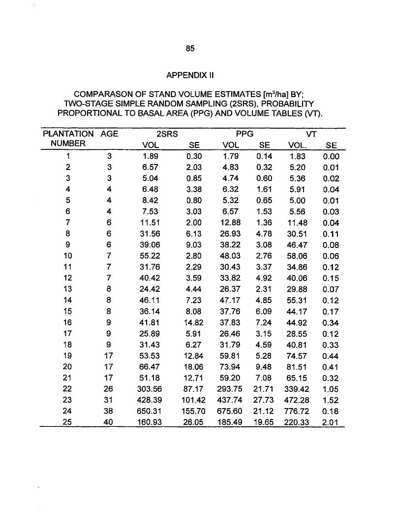
COMPARASON OF STAND VOLUME ESTIMATES [m3/ha] BY; TWO-STAGE SIMPLE RANDOM SAMPLING (2SRS), PROBABILJTY

PROPORTIONAL TO BASAL AREA (PPG) AND VOLUME TABLES (VT).

PLANTATION AGE 2SRS PPG VT NUMBER VOL SE VOL SE VOL. SE

APPENDIX III

ABOVEGROUND STAND BlOMASS ESTIMATES [thal

PLANTATION AGE COMPONENT BIOMASS (t /ha) NUMBER STEM BRANCH LMVE TOTAL

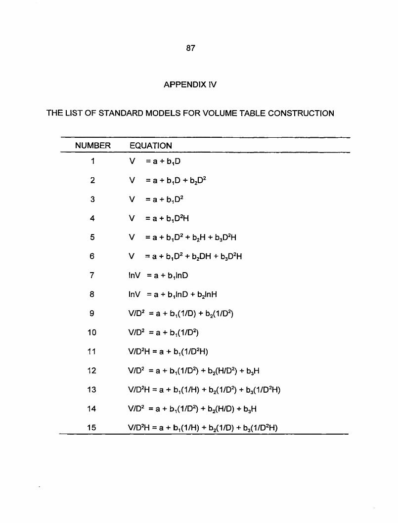
APPENDIX IV

THE LIST OF STANDARD MODELS FOR VOLUME TABLE CONSTRUCTION

NUMBER EQUATION . . . - - - - -. - -

1 V =a+b,D

2 V =a+b,D+b,D2

3 V =a+b,D2

4 V =a+b,DZH

5 V = a + b,D2 + b,H + b,D2H

6 V = a + b,D2 + $DH + b3D2H

7 InV = a + bllnD

8 InV = a + b,hD + b,lnH

9 V/D2 = a + b,(ilD) + b,(l/D2)

1 O VlD2 = a + b,(l/D2)

? 1 V/D2H = a + b,(l/D2H)

12 V/D2 = a + b1(l/D2) + b2(HID2) + b,H

13 V/D2H = a + b,(l IH) + b2(l ID2) + b3(l /D2H)

14 V/D2 = a + b,(l/D2) + bdH/D) + b,H

15 VID2H = a + b,(l /H) + b2(l/D) + b3(l /D2H)

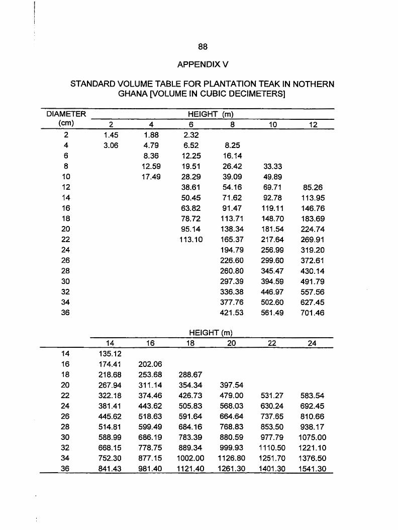
APPENDIX V

STANDARD VOLUME TABLE FOR PLANTATION TEAK IN NOTHERN GHANA VOLUME IN CUBlC DECIMETERS]

DIAMETER HEIGHT (ml

HEIGHT (rn) 14 16 18 20 22 24

14 135.12 16 1 74.41 202.06

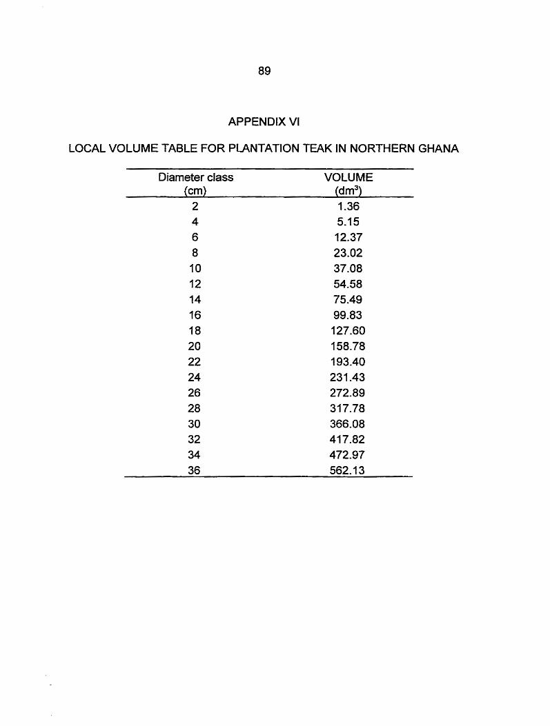
APPENDIX VI

LOCAL VOLUME TABLE FOR PLANTATION TEAK IN NORTHERN GHANA

Diameter class VOLUME (cm) (dm3) 2 1.36

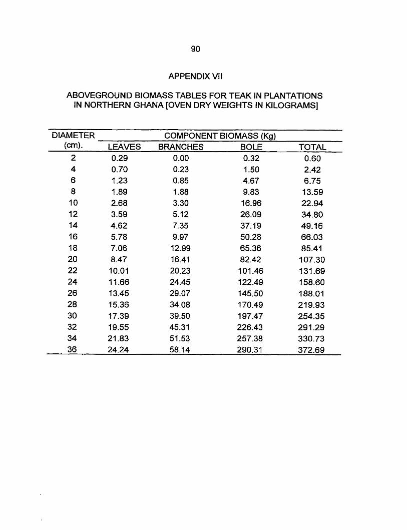
ABOVEGROUND BlOMASS TABLES FOR TEAK IN PiANTATlONS IN NORTHERN GHANA [OVEN DRY WEIGHTS IN KILOGRAMS]

DIAMETER COMPONENT BlOMASS (Kg) LEAVES BRANCHES BOLE TOTAL

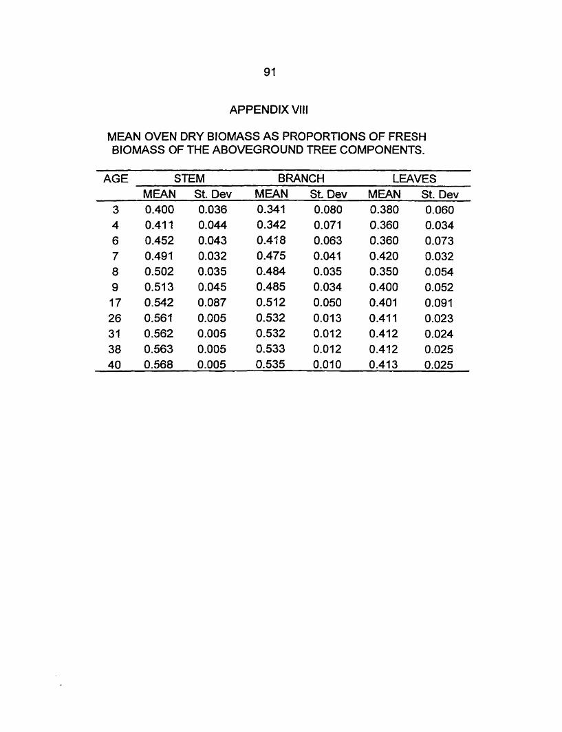
MEAN OVEN DRY BlOMASS AS PROPORTIONS OF FRESH BIOMASS OF THE ABOVEGROUND TREE COMPONENTS.

AGE STEM BRANCH LEAVES MEAN St. Dev MEAN St. Dev MEAN St. Dev

3 0.400 0.036 0.341 0.080 0.380 0.060

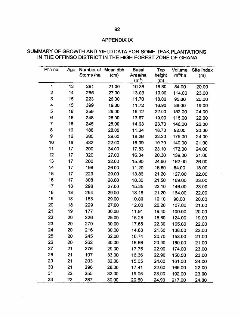
SUMMARY OF GROWTH AND YIELD DATA FOR SOME TEAK PLANTATIONS IN THE OFFINSO DISTRICT IN THE HlGH FOREST ZONE OF GHANA

Pl'n no. Age Number of Mean dbh Basal Top Volume Site Index Stems /ha (cm) Arealha heig hi m3/ha (m)

(m2) (m)

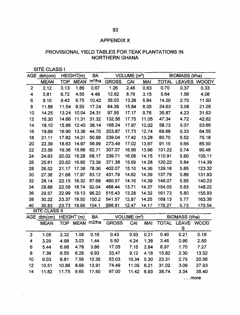
APPENDIX X

PROVISIONAL YlELD TABLES FOR T€AK PLANTATIONS IN NORTHERN GHANA

SlTE CWSS I ---

AGE dbh(cm) HEIGHT(m) BA VOLUME (m3) BIOMASS (tlha) MEAN TOP MEAN m 2 h GROSS CA1 MAI TOTAL LEAVES WOODY

. 30.83 23.73 19.85 104.1 566.91 12.47 14.17 176.27 5.73 î70.54 SlTE CLASS II

AGE dbh(cm) HEtGHT(m) BA -- VOLUME (m3) BIOMASS (üha)

MEAN TOP MEAN m2fha GROSS CA1 MAI TOTAL LEAVE WOOD

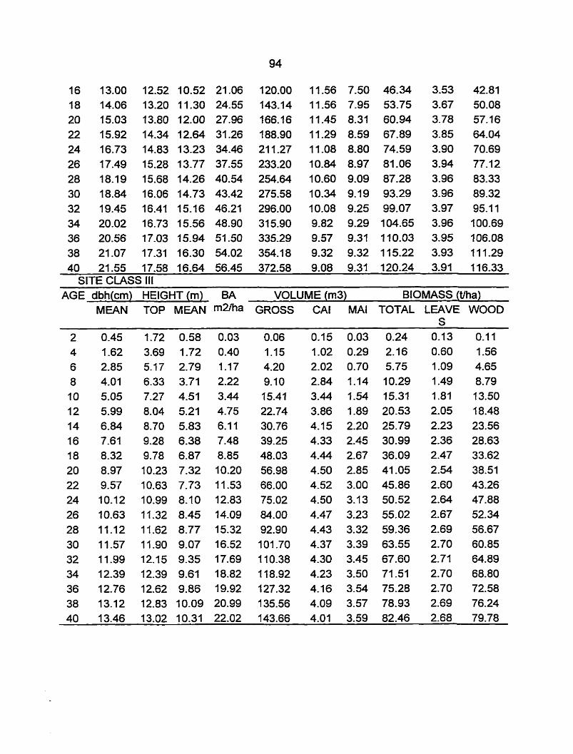
21 -55 17.58 16.64 56.45 372.58 9.08 9-31 120.24 3.91 116.33 SITE CLASS III

AGE dbh(cm) HElGHT(m) BA VOLUME (m3) B IOMASS (tlha) MEAN TOP MEAN maha GROSS CA1 MAI TOTAL LEAVE WOOD

S

APPENDIX XI

OBSERVED AND PREDICTED DIAMETER CLASS FREQUENCIES BY AGE CLASSES

AG€ CLASS DIAMETER DIAMETER FREQUENCIES (PER HACTARE) CUSS (cm) OBSERVED PRED (PT) PRED. (ML)

3 YEAR 1 27 28 21 2 650 682 649 3 567 558 553 4 260 234 265 5 63 67 79 6 16 14 16

TOTAL 1583 1583 1583

4 YEAR 1 22 18 16 2 314 501 310 3 643 61 7 717 4 449 349 424 5 173 117 130 6 22 25 25 7 5 3 6 9 2 O 2

TOTAL 1630 1630 1630

6 YEAR 2 22 18 23 3 135 165 136 4 449 363 429 5 406 455 455 6 384 437 407 7 384 346 320 8 271 233 227 9 89 135 136 10 65 68 70 II 49 30 45 12 5 12 13

TOTAL 2260 2260 2260

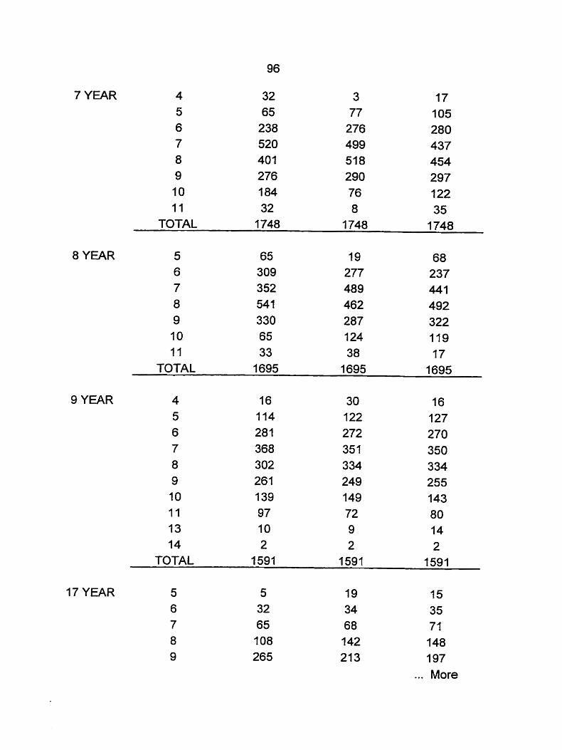
7 YEAR

8 YEAR

9 YEAR

17 YEAR

4 32 3 17 5 65 77 1 05 6 238 276 280 7 520 499 437 8 401 518 454 9 276 290 297 IO 184 76 122 I I 32 8 35

TOTAL 1748 1748 1748

5 65 19 68 6 309 277 237 7 352 489 441 8 541 462 492 9 330 287 322 IO 65 124 119 1 I 33 38 17

TOTAL 1695 1695 1695

4 16 30 16 5 114 'l22 127 6 281 272 270 7 368 35 1 350 8 302 334 334 9 261 249 255 IO 139 149 143 1 1 97 72 80 13 10 9 14 14 2 2 2

TOTAL 1591 1591 1591

15 35 71 148 197

... More

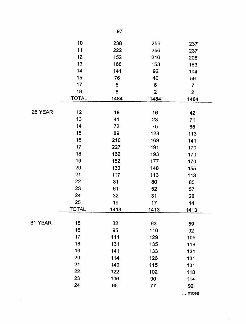
I O 238 256 237 11 222 256 237 12 152 216 208 13 168 153 163 14 141 92 1 04 15 76 46 59 17 6 6 7 18 5 2 2

TOTAL 1484 1484 1484

26 YEAR 12 19 16 42 13 41 23 71 14 72 75 85 15 89 128 113 16 210 169 141 17 227 191 170 18 162 193 170 19 152 177 170 20 130 148 155 21 117 113 113 22 81 80 85 23 61 52 57 24 32 31 28 25 19 17 14

TOTAL 1413 1413 1413

31 YEAR 15 16 17 18 19 20 21 22 23 24

59 92 1 O5 118 131 131 131 118 I l 4 92

... more

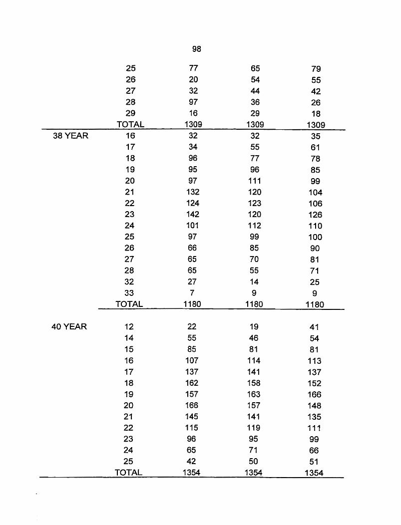
TOTAL 1309 1309 1309 38 YEAR 16 32 32 35

TOTAL 1180 1180 1180

40 YEAR 12 22 19 41 14 55 46 54 15 85 81 81 76 1 07 114 113 17 137 141 137 18 162 158 152 19 157 163 166 20 166 157 148 21 145 141 135 22 115 119 11 7 23 96 95 99 24 65 71 66 25 42 50 51

TOTAL 1354 1354 1354

SITE INDEX CURVES OF TEAK PLANTATIONS IN NORTHERN GHANA

1 O0

APPENDIX Xlll

VOLUME GROVVTH CURVES FOR TEAK PLANTATIONS IN NORTHERN GHANA

O 10 20 30 40 50

AGE

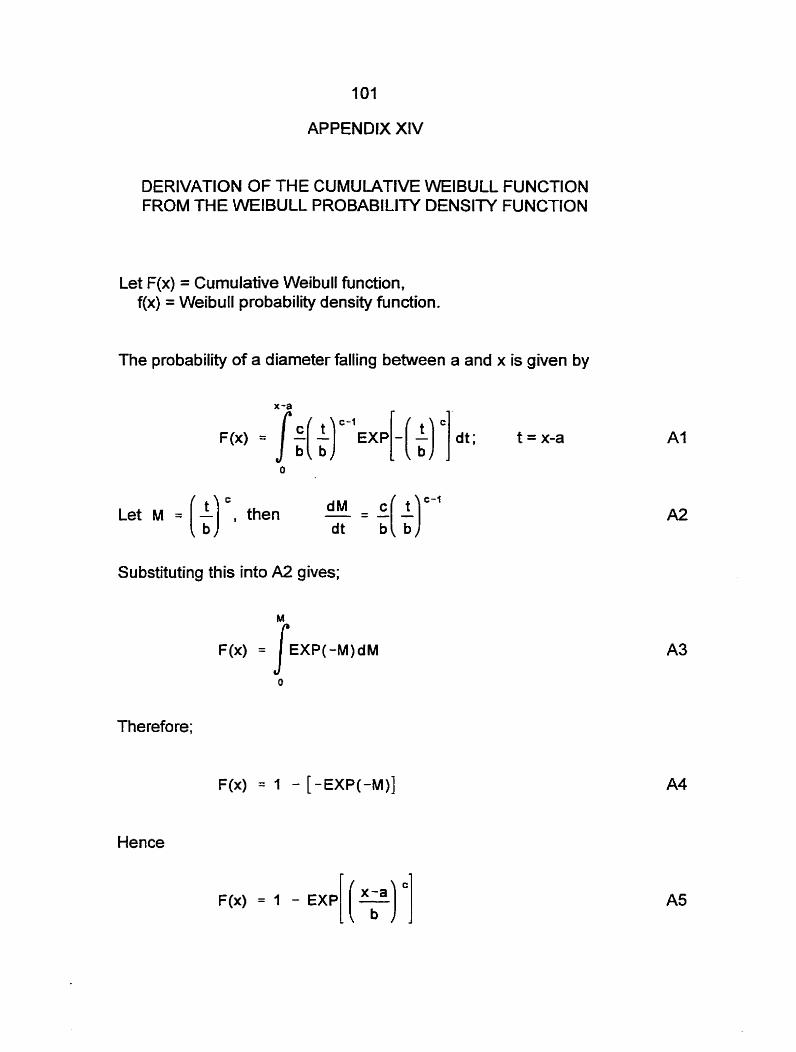
I O 1

APPENDIX XIV

DERIVATION OF THE CUMULATIVE WEIBULL FUNCTlON FROM THE WElBULL PROBABILIlY DENSIW FUNCTlON

Let F(x) = Cumulative Weibull function, f(x) = Weibull probability density function.

The probability of a diameter falling between a and x is given by

x-a

Let M = ( $) ', then

Substituting this into A2 gives;

Therefore;

F(X) = I - [-EXP(-MI]

Hence

] cit; t = x-a

IMAGE EVALUATION TEST TARGET (QA-3)

APPLIED I M G E . lnc - = 1653 East Main Street - -. - Rochester. NY 14609 USA -- -- - - Phone: 716/482-0300 -- -- - - F a 71 6128û-5989