Gradient Projection Anti-windup Scheme

by

Chun Sang Justin Teo

B.Eng. Electrical and Electronic EngineeringNanyang Technological University, 1999

M.Sc. Electrical EngineeringNational University of Singapore, 2003

Submitted to the Department of Aeronautics and Astronauticsin partial fulfillment of the requirements for the degree of

Doctor of Science

at the

MASSACHUSETTS INSTITUTE OF TECHNOLOGY

February 2011

c© 2011 Chun Sang Justin Teo. All rights reserved.

The author hereby grants to MIT permission to reproduce and to distribute publiclypaper and electronic copies of this thesis document in whole or in part in any

medium now known or hereafter created.

Author . . . . . . . . . . . . . . . . . . . . . . . . . . . . . . . . . . . . . . . . . . . . . . . . . . . . . . . . . . . . . . . . . . . . . . . . . . . .Department of Aeronautics and Astronautics

December 29, 2010

Certified by. . . . . . . . . . . . . . . . . . . . . . . . . . . . . . . . . . . . . . . . . . . . . . . . . . . . . . . . . . . . . . . . . . . . . . . .Jonathan Patrick How

Richard C. Maclaurin Professor of Aeronautics and AstronauticsThesis Supervisor

Certified by. . . . . . . . . . . . . . . . . . . . . . . . . . . . . . . . . . . . . . . . . . . . . . . . . . . . . . . . . . . . . . . . . . . . . . . .Emilio Frazzoli

Associate Professor of Aeronautics and Astronautics

Certified by. . . . . . . . . . . . . . . . . . . . . . . . . . . . . . . . . . . . . . . . . . . . . . . . . . . . . . . . . . . . . . . . . . . . . . . .Steven Ray Hall

Professor of Aeronautics and AstronauticsMacVicar Faculty Fellow

Certified by. . . . . . . . . . . . . . . . . . . . . . . . . . . . . . . . . . . . . . . . . . . . . . . . . . . . . . . . . . . . . . . . . . . . . . . .Eugene Lavretsky

Senior Technical Fellow, The Boeing Company

Accepted by . . . . . . . . . . . . . . . . . . . . . . . . . . . . . . . . . . . . . . . . . . . . . . . . . . . . . . . . . . . . . . . . . . . . . . .Eytan Modiano

Associate Professor of Aeronautics and AstronauticsChair, Graduate Program Committee

Gradient Projection Anti-windup Schemeby

Chun Sang Justin Teo

Submitted to the Department of Aeronautics and Astronauticson December 29, 2010, in partial fulfillment of the

requirements for the degree ofDoctor of Science

Abstract

It is a well-recognized fact that control saturation affects virtually all practical controlsystems. It leads to controller windup, which degrades/limits the system’s closed-loop per-formance, and may cause catastrophic failures if it induces instability. Anti-windup compen-sation is one of two main approaches to mitigate the effects of windup, and is conceptuallyand practically attractive. For the idealized case of constrained linear time invariant (LTI)plants driven by LTI controllers, numerous anti-windup schemes exist. However, most prac-tical control systems are inherently nonlinear, and anti-windup compensation for nonlinearsystems remains largely an open problem.

To this end, we propose the gradient projection anti-windup (GPAW) scheme, which isan extension of the conditional integration method to multi-input-multi-output (MIMO)nonlinear systems, using Rosen’s gradient projection method for nonlinear programming.It achieves controller state-output consistency by projecting the controller state onto theunsaturated region induced by the control saturation constraints. The GPAW-compensatedcontroller is a hybrid controller defined by the online solution to either a combinatorial opti-mization subproblem, a convex quadratic program, or a projection onto a convex polyhedralcone problem. We show that the GPAW-compensated system is obtained by modifying theuncompensated system with a passive operator.

Qualitative weaknesses of some existing anti-windup results are established, which moti-vated a new paradigm to address the anti-windup problem. It is shown that for a constrainedfirst order LTI plant driven by a first order LTI controller, GPAW compensation can onlymaintain/enlarge its region of attraction (ROA). In this new paradigm, we derived someROA comparison and stability results for MIMO nonlinear as well as MIMO LTI systems.

The thesis is not that the GPAW scheme solves a centuries-old open problem of immensepractical importance, but rather, that it provides a potential path to a solution. We invitethe reader to join us in this quest at the confluence of nonlinear systems, hybrid systems,projected dynamical systems, differential equations with discontinuous right-hand sides,combinatorial optimization, convex analysis and optimization, and passive systems.

Thesis Supervisor: Jonathan Patrick HowTitle: Richard C. Maclaurin Professor of Aeronautics and Astronautics

To my three lovely, sweet, mischievous ladies,Linee, Sonya, Clara

and not forgetting my confidante,Kakuni

Preface

I surmise that readers of doctoral dissertations are motivated by a desire to find a morecoherent treatment of the subject matter that may have been scattered across numerouspublications, and that readers of prefaces of doctoral dissertations are interested in how thesubject matter developed or evolved. Here, I provide a candid reflection of how the gradientprojection anti-windup (GPAW) scheme came about, almost by accident.

I started the doctoral program at MIT’s Department of Aeronautics and Astronautics inthe fall of 2005, working with my advisor Prof. Jonathan P. How (or Jon) ever since. Initialtinkering with parallel optimization based trajectory planning leads to nowhere. Then camethe Defense Advanced Research Projects Agency (DARPA) Urban Challenge1 where I spenta very memorable period (Jun. 2006 to Dec. 2007) with a highly energized team developingthe controller and Rapidly-Exploring Random Tree (RRT) based trajectory planner2 forMIT’s entry. However, nothing resembling a doctoral dissertation that truly interests mecan be made out of it. I started looking into adaptive control, which occupied me for thenext year or so. Although resulting in a journal technical note3 (that has nothing to do withadaptive control), that line of research also fell somewhat short of a doctoral dissertation.By the fall of 2008, I was in a somewhat desperate state, being without a concrete thesistopic, and with funding for my doctoral studies4 scheduled to run out in a year.

Then, as part of the process of catching up on coursework (after the neglect owing inno small part to involvement in the DARPA Urban Challenge), I took the class “Non-linear Control System Design” by Prof. Jean-Jacques E. Slotine in the fall of 2008. Theclass requires completion of a project, for which I chose to study how prior knowledge ofbounds on system parameters can be incorporated in an adaptive controller (that requiresno such knowledge). Intuitively, incorporating the knowledge of such bounds can improvethe system’s performance, which I showed in the project report. Not surprisingly, it turnedout that Prof. Slotine had proved similar and more general results two decades ago. Thebounds on the system parameters I studied are interval bounds, so that the bounded re-gion containing the unknown system parameters are cuboids. Considering more generalbounding conditions, e.g. bounds imposed by a set of nonlinear inequalities, proved elusive,at least for the class project. A class project is nice in the sense that, unlike a researchpaper, reporting on negative results, like my unsuccessful attempt to generalize the resultsto regions defined by nonlinear inequalities, is acceptable. After my project presentation,numerous discussions with Prof. Slotine led me to projection methods for adaptive control5

that have been used to bound estimates of system parameters in some a priori known re-gion. However, such projection methods are limited to projection with respect to a singlenonlinear inequality, in contrast to a system of nonlinear inequalities. To summarize, we

1The DARPA Urban Challenge (see http://www.darpa.mil/grandchallenge and http:

//grandchallenge.mit.edu) is a competition where autonomous robots are required to complete amock mission in a suburban environment while obeying some basic traffic rules.

2Y. Kuwata, J. Teo, G. Fiore, S. Karaman, E. Frazzoli, and J. P. How, “Real-time motion planning withapplications to autonomous urban driving,” IEEE Trans. Control Syst. Technol., vol. 17, no. 5, pp. 1105 –1118, Sep. 2009.

3J. Teo, J. P. How, and E. Lavretsky, “Proportional-Integral Controllers for Minimum-Phase Nonaffine-in-Control Systems,” IEEE Trans. Autom. Control, vol. 55, no. 6, pp. 1477 – 1483, Jun. 2010.

4By my employer and sponsor, DSO National Laboratories, Singapore, for which I am deeply grateful.In May 2009, 4 months to the original schedule where my funding was to run out, DSO extended fundingfor doctoral studies to 5 years (for me, ending in Sep. 2010), at a very much needed and opportune time.

5In P. A. Ioannou and J. Sun, Robust Adaptive Control. Upper Saddle River, NJ: Prentice Hall, 1996.[Online]. Available: http://www-rcf.usc.edu/~ioannou/Robust_Adaptive_Control.htm.

7

can project onto cuboid type regions or regions defined by a single nonlinear inequality, butnot regions defined by multiple nonlinear inequalities.

The state of affairs being thus unsatisfactory, the natural progression is to attempt toextend the projection method of Ioannou and Sun to handle multiple nonlinear inequali-ties. This led me to the venerable gradient projection method for nonlinear programming6

proposed by Rosen in 1960. In analogy to Ioannou and Sun’s projection method, whatwas required is the extension of Rosen’s gradient projection method to continuous time.Then the resulting projection mechanism (less the optimization part) allows projection ofthe adaptive control parameter estimates onto any region defined by a system of nonlinearinequalities. And so I went ahead and extended Rosen’s method to continuous time.7

At that time, my prior experience as a control engineer with DSO National Laboratoriesmade me realize that the same projection mechanism that can be used to bound parameterestimates in adaptive control, can be used in an anti-windup setting to achieve controllerstate-output consistency, i.e. to modify the controller state such that its output inherentlysatisfy the saturation constraints. This is easily seen by observing that the projectionmechanism allows the projection of the controller state onto any region defined by a systemof nonlinear inequalities, and that controller state-output consistency simply requires thecontroller state to remain in some region defined by a system of saturation constraintinequalities. The obvious thing to do next is to confirm this intuition in simulation, whichis easily done. Simulations on an input-constrained two-link robot driven by an adaptivesliding mode controller (made familiar in Prof. Slotine’s class) yields very promising resultswith little to no tweaking. On reflection, all I had done was simply used an extension ofRosen’s (1960) method to extend the conditional integration anti-windup scheme that haslong been adopted by practitioners for proportional-integral-derivative type controllers.

At this point in time (probably around Jan. 2009), I was clueless as to the magnitude ofwhat I had stumbled on. I was aware that anti-windup compensation is a well researchedtopic. But hard as I try, I could not find any literature that treats general nonlinearsystems.8 It was only a few weeks later when I chanced on a survey paper on anti-windupcompensation9 that I realized that anti-windup compensation for nonlinear systems is stillconsidered an open problem. This got me really excited, as I have finally found a topicworthy of a doctoral dissertation.

The next period up to the submission date for the IEEE Conference on Decision andControl (around Mar. 2009) was spent writing up these initial results. When the conferencepaper10 was submitted, reality set in. Euphoria gave way to helplessness, when I realizedI had created a beast that I need to tame in order to graduate, without the slightest clueon how to go about it. I felt like Victor Frankenstein11 after successfully giving life to his

6J. B. Rosen, “The gradient projection method for nonlinear programming. part I. linear constraints,”J. Soc. Ind. Appl. Math., vol. 8, no. 1, pp. 181 – 217, Mar. 1960.

7Without bothering much about whether it actually solves the underlying optimization problem. Nu-merical results suggest that it does. Since my interest lies entirely on only the projection mechanism, I leavethe proofs to the continuous optimization community if it manages to generate any interest.

8I have only found literature applicable to feedback linearizable nonlinear systems and Euler-Lagrangesystems.

9S. Tarbouriech and M. Tuner, “Anti-windup design: an overview of some recent advances and openproblems,” IET Control Theory Appl., vol. 3, no. 1, pp. 1 – 19, Jan. 2009.

10J. Teo and J. P. How, “Anti-windup compensation for nonlinear systems via gradient projection: Appli-cation to adaptive control,” in Proc. 48th IEEE Conf. Decision and Control & 28th Chinese Control Conf.,Shanghai, China, Dec. 2009, pp. 6910 – 6916.

11M. W. Shelley, Frankenstein: or, The Modern Prometheus. London, England: Thomas Davison, 1823.[Online]. Available: http://books.google.com/books?id=5twBAAAAQAAJ.

8

monster. Just to reflect on the magnitude of the task at hand, recall that the problem ofcontrol saturation existed since the dawn of control theory, since James Watt’s governor wasinvented. For linear time invariant (LTI) systems, rigorous stability results for anti-windupschemes were obtained only from the late 1990s onwards. We have here a centuries-old openproblem of immense practical importance, compounded by the complexities of nonlinearsystems! Even for the controls gurus, (I suspect) this would have been daunting, andsignificantly more so for a panicky struggling graduate student with 6 months left beforefunding runs out.

In the face of a seemingly insurmountable task, the wisdom of Jon (my advisor) isrevealed when he insisted that I look at the simplest possible feedback system, i.e. aninput-constrained first order LTI plant driven by a first order LTI controller. Naturally, Iwas skeptical. How much can the simplest system reveal, when perhaps all there is to knowis already known, and our objective is on the opposite end of the spectrum? Contrary tomy initial pessimism, it turns out that a whole lot can be revealed, and the practitioner’sad hoc conditional integration method12 can only maintain/enlarge the system’s regionof attraction (ROA), and is likely an optimal anti-windup scheme in the sense that noother anti-windup scheme can achieve a larger ROA. The culmination of this exercise is atechnical report13 and a (derivative) conference paper.14 It surprised me that practitionershad developed a (likely) optimal anti-windup scheme perhaps without knowing the fullpower of what they had developed! Even more astounding (to me) is the amount of insightsthat this simple system (that I had formerly “despised”) had revealed, which led indirectlyto the rest of the development presented in this dissertation. The single-minded pursuit ofthis generalization of a decades-old method led me into areas as diverse as hybrid systems,projected dynamical systems,15 differential equations with discontinuous right-hand sides,combinatorial optimization, convex analysis and optimization, passivity, and more.

This is the story of how the GPAW scheme arose from a class project, in perhaps someof the most unlikely circumstances brought about by a great deal of luck and coincidences(and of course, hard work). Through these, I learned that it pays to pursue any trainof thought wholeheartedly without compromise, and that no system is too simple to beunworthy of study.

Obviously, my first thanks goes to my advisor Prof. Jonathan P. How. His ability tosee through a complex sequence of operations and condense it into a one-liner is amazing.From Jon, I learned to ask the right questions, and to pursue a train of thought even if itis controversial and politically incorrect. He showed me how to build up an argument, andmost of all, taught me what research is all about.16

My thesis committee members, Prof. Emilio Frazzoli, Prof. Steven R. Hall, and Dr. Eu-gene Lavretsky, have been instrumental in providing constructive criticism and feedback,

12The GPAW scheme, being the extension of the conditional integration method, naturally reduces to theconditional integration method for this simple system.

13J. Teo and J. P. How, “Gradient projection anti-windup scheme on constrained planar LTI systems,”MIT, Cambridge, MA, Tech. Rep. ACL10-01, Mar. 2010, Aerosp. Controls Lab. [Online]. Available: http://hdl.handle.net/1721.1/52600.

14J. Teo and J. P. How, “Analysis of gradient projection anti-windup scheme,” in Proc. American ControlConf., Baltimore, MD, Jun./Jul. 2010, pp. 5966 – 5972.

15Projected dynamical systems is a significant line of independent research that has attracted the attentionof mathematicians, physicists, and economists, among others.

16It may seem obvious to many people, but on hindsight, I was not doing independent research until re-cently. There came a point in time when I realized that I was constantly formulating non-obvious conjecturesand then proving or disproving them. Only then do I consider myself doing research.

9

and steering my research to completion. It has been an honor to have them on my commit-tee. From Emilio, I learned a great deal about RRTs during the DARPA Urban Challengephase. Collaboration with Dr. Lavretsky on approximate dynamic inversion17 accustomedme to singular perturbation theory, a key element needed to extend the GPAW results tosystems driven by nonlinear controllers of general structure.

I am indebted to Prof. Jean-Jacques E. Slotine for seeding the crucial initial thoughtsthat led to the development of the GPAW scheme. Without his leads, this dissertationwould be non-existent. His lectures are always insightful, as reflected in his book, “AppliedNonlinear Control,” one of the few that I have read cover-to-cover. I also thank Dr. LouisBreger and Dr. Luca Bertucelli for being my dissertation readers.

Generous financial support from my employer and sponsor DSO National Laboratories,Singapore, has enabled my doctoral studies to progress without me having to worry too muchon the means to provide for my family. The freedom to choose a thesis topic to my likingis a luxury not afforded to all doctoral candidates, but enabled by the DSO PostgraduateScholarship. For these, I am deeply grateful, especially the extension of funding for doctoralstudies at the most opportune time.

Involvement in the DARPA Urban Challenge has been one of the most memorable andintense phases of my MIT experience. Many days (and nights), some filled with exhilaration,many more filled with disappointment, were spent in deserted air bases with Dr. YoshiakiKuwata, Gaston Fiore, Stefan Campbell, Sertac Karaman, Andrew Patrikalakis, Dr. LukeFletcher, Prof. Edwin Olson, David Moore, and Dr. Albert Huang, working on a Land Roverthat in totality costs more than a Ferrari. The principal investigators, Prof. John Leonard,Prof. Jonathan P. How, Prof. Seth Teller, and Prof. David Barrett (of Olin College) havedone a wonderful job which enabled our 4th place finishing, something I will continue toboast about for quite some time.

Kathryn Fischer has been most helpful throughout my 5 years at MIT, always ensuringthat Aerospace Controls Laboratory (ACL) members have what they need, and always witha smile. When she works her magic, what would have taken weeks to accomplish reducesto mere hours. Her resourceful assistance will be remembered with much gratitude.

Members of ACL past and present have contributed positively to my MIT experience.I mention Dr. Yoshiaki Kuwata, Gaston Fiore, Prof. Han-Lim Choi, Dr. Louis Breger, Dr.Luca Bertucelli, Prof. Emily Craparo, Dr. Mehdi Alighanbari, Georges Aoude, Dr. GeoffreyHuntington, and Henry Jacques Lefebvre de Plinval-Salgues, all of whom once shared anoffice with me in the “Laboratory for Random Graduate Students”.

Last, but certainly not least, my thanks goes to my family. My parents Johny Teo andChan Gian Hoe have always been supportive, through my rebellious teenage years to thepresent. Fatherhood made me aware of the sacrifices they must have made and the trialsthey must have gone through. My heartfelt thanks goes to them for molding me into whoI am. My wife Linee Yeo sacrificed a good career with great prospects and a job she lovedthat is better-paid than mine, to allow me the luxury of pursuing doctoral studies at MIT.She is the caregiver, disciplinarian, comforter, entertainer, activity planner, cook, driver,art and craft teacher, story teller, and more, to our two daughters Sonya and Clara. Sheshouldered much of the parenting task so that I can focus on my research. For these andmany more untold sacrifices, as well as the love and companionship, I am infinitely grateful.

Cambridge, MA, November 2010 Justin Teo

17N. Hovakimyan, E. Lavretsky, and A. Sasane, “Dynamic inversion for nonaffine-in-control systems viatime-scale separation. Part I,” J. Dyn. Control Syst., vol. 13, no. 4, pp. 451 – 465, Oct. 2007.

10

Contents

1 Introduction 19

1.1 Control Design Strategies for Input-constrained Systems . . . . . . . . . . . 20

1.2 Anti-windup Compensation . . . . . . . . . . . . . . . . . . . . . . . . . . . 21

1.2.1 Anti-windup Compensation for Nonlinear Systems – Open Problem 22

1.3 Problem Statement . . . . . . . . . . . . . . . . . . . . . . . . . . . . . . . . 23

1.3.1 Recovering the Anti-windup Compensator . . . . . . . . . . . . . . . 25

1.4 Literature Review . . . . . . . . . . . . . . . . . . . . . . . . . . . . . . . . 26

1.4.1 Conditioning Technique . . . . . . . . . . . . . . . . . . . . . . . . . 26

1.4.2 Feedback Linearizable Nonlinear Systems . . . . . . . . . . . . . . . 27

1.4.3 Anti-windup Schemes for Particular Controllers . . . . . . . . . . . . 27

1.4.4 Nonlinear Anti-windup for Euler-Lagrange Systems . . . . . . . . . . 27

1.4.5 Optimal Directionality Compensation . . . . . . . . . . . . . . . . . 28

1.4.6 Reference Governor . . . . . . . . . . . . . . . . . . . . . . . . . . . 29

1.4.7 Summary of Literature Review . . . . . . . . . . . . . . . . . . . . . 29

1.5 Dissertation Overview . . . . . . . . . . . . . . . . . . . . . . . . . . . . . . 30

1.6 Contributions . . . . . . . . . . . . . . . . . . . . . . . . . . . . . . . . . . . 32

2 Construction and Fundamental Properties 33

2.1 Conditional Integration . . . . . . . . . . . . . . . . . . . . . . . . . . . . . 33

2.2 Gradient Projection Method for Nonlinear Programming . . . . . . . . . . . 36

2.3 Continuous Time Gradient Projection Method . . . . . . . . . . . . . . . . 38

2.3.1 Scaled Continuous Time Gradient Projection Method . . . . . . . . 42

2.4 Projection Operator . . . . . . . . . . . . . . . . . . . . . . . . . . . . . . . 43

2.5 Gradient Projection Anti-windup (GPAW) Scheme . . . . . . . . . . . . . . 46

2.6 Approximate Nominal Controller . . . . . . . . . . . . . . . . . . . . . . . . 53

2.7 Passivity and L2-Gain of Projection Operator . . . . . . . . . . . . . . . . . 56

2.8 GPAW Compensation on a Two-link Robot Driven by an Adaptive SlidingMode Controller . . . . . . . . . . . . . . . . . . . . . . . . . . . . . . . . . 59

2.8.1 Approximate Nominal Controller . . . . . . . . . . . . . . . . . . . . 61

2.8.2 GPAW-Compensated Controller . . . . . . . . . . . . . . . . . . . . 63

2.8.3 Constrained Control . . . . . . . . . . . . . . . . . . . . . . . . . . . 64

2.8.4 Numerical Results . . . . . . . . . . . . . . . . . . . . . . . . . . . . 66

2.9 Relations with Existing Methods . . . . . . . . . . . . . . . . . . . . . . . . 69

2.10 Chapter Summary . . . . . . . . . . . . . . . . . . . . . . . . . . . . . . . . 70

11

3 Input Constrained Planar LTI Systems 73

3.1 Preliminaries . . . . . . . . . . . . . . . . . . . . . . . . . . . . . . . . . . . 74

3.2 GPAW-Compensated System as a Projected Dynamical System . . . . . . . 78

3.3 Existence and Uniqueness of Solutions . . . . . . . . . . . . . . . . . . . . . 79

3.4 Existence of Multiple Equilibria . . . . . . . . . . . . . . . . . . . . . . . . . 82

3.5 Region of Attraction . . . . . . . . . . . . . . . . . . . . . . . . . . . . . . . 84

3.5.1 ROA Containment in Unsaturated Region . . . . . . . . . . . . . . . 85

3.5.2 ROA Containment in Saturated Region . . . . . . . . . . . . . . . . 89

3.5.3 Main Result . . . . . . . . . . . . . . . . . . . . . . . . . . . . . . . . 92

3.5.4 Numerical Results . . . . . . . . . . . . . . . . . . . . . . . . . . . . 93

3.6 Illustration of the Need to Consider Asymmetric Saturation Constraints . . 94

3.7 A Paradigm Shift in Anti-windup Compensation . . . . . . . . . . . . . . . 96

3.8 Relation to the General Anti-windup Problem . . . . . . . . . . . . . . . . . 98

3.9 Solution Bounce Property and Some Conjectures . . . . . . . . . . . . . . . 99

3.10 Chapter Summary . . . . . . . . . . . . . . . . . . . . . . . . . . . . . . . . 101

3.11 Chapter Supplement . . . . . . . . . . . . . . . . . . . . . . . . . . . . . . . 102

3.11.1 Translating Some Logical Statements . . . . . . . . . . . . . . . . . . 102

3.11.2 A Variant of the Comparison Lemma . . . . . . . . . . . . . . . . . . 102

3.11.3 Proofs of Intermediate Results for Section 3.5.1 . . . . . . . . . . . . 103

3.11.4 Proofs of Intermediate Results for Section 3.5.2 . . . . . . . . . . . . 107

4 Geometric Properties and Region of Attraction Comparison Results 113

4.1 Quadratic Program Formulation of GPAW-Compensated Controllers . . . . 113

4.1.1 Initializing the Quadratic Program . . . . . . . . . . . . . . . . . . . 117

4.2 A Geometric Bounding Condition . . . . . . . . . . . . . . . . . . . . . . . . 118

4.3 A General Region of Attraction Comparison Result . . . . . . . . . . . . . . 122

4.4 Region of Attraction Comparison for GPAW-Compensated Systems . . . . 125

4.5 Applications of Region of Attraction Comparison Results . . . . . . . . . . 132

4.5.1 Input Constrained Planar LTI Systems . . . . . . . . . . . . . . . . . 132

4.5.2 A Nonlinear Example for Application of Theorem 4.4.1 . . . . . . . 135

4.6 Chapter Summary . . . . . . . . . . . . . . . . . . . . . . . . . . . . . . . . 137

5 Input Constrained MIMO LTI Systems 139

5.1 System Descriptions . . . . . . . . . . . . . . . . . . . . . . . . . . . . . . . 139

5.2 A Stability Result for Systems with Open-loop Stable Plants . . . . . . . . 142

5.2.1 Numerical Example . . . . . . . . . . . . . . . . . . . . . . . . . . . 144

5.3 GPAW-Compensated Controller Transformations . . . . . . . . . . . . . . . 146

5.4 Linear Systems with Partial State Constraints . . . . . . . . . . . . . . . . . 149

5.5 A Canonical Form for GPAW Compensation . . . . . . . . . . . . . . . . . 149

5.5.1 Full Row Rank Cc . . . . . . . . . . . . . . . . . . . . . . . . . . . . 150

5.5.2 Row Rank Deficient Cc . . . . . . . . . . . . . . . . . . . . . . . . . 150

5.5.3 Comments on Nominal Controller Transformations . . . . . . . . . . 152

5.6 A Relation between GPAW-Compensated LTI Systems and Linear Systemswith Partial State Constraints . . . . . . . . . . . . . . . . . . . . . . . . . . 152

5.6.1 Illustration of an Existing Result . . . . . . . . . . . . . . . . . . . . 159

5.7 Chapter Summary . . . . . . . . . . . . . . . . . . . . . . . . . . . . . . . . 160

12

6 Numerical Comparisons 1616.1 Nonlinear Anti-windup Scheme . . . . . . . . . . . . . . . . . . . . . . . . . 161

6.1.1 Nonlinear Anti-windup Compensated System . . . . . . . . . . . . . 1626.1.2 Approximate Nominal System . . . . . . . . . . . . . . . . . . . . . . 1626.1.3 GPAW-Compensated System . . . . . . . . . . . . . . . . . . . . . . 1636.1.4 Numerical Results . . . . . . . . . . . . . . . . . . . . . . . . . . . . 164

6.2 Two Anti-windup Schemes for Nonlinear Systems . . . . . . . . . . . . . . . 1646.2.1 Feedback Linearized Anti-windup Compensated System . . . . . . . 1656.2.2 Nonlinear Anti-windup Compensated System . . . . . . . . . . . . . 1666.2.3 Approximate Nominal System . . . . . . . . . . . . . . . . . . . . . . 1676.2.4 GPAW-Compensated System . . . . . . . . . . . . . . . . . . . . . . 1676.2.5 Numerical Results . . . . . . . . . . . . . . . . . . . . . . . . . . . . 168

6.3 LMI-based Anti-windup Scheme for Stable LTI Systems . . . . . . . . . . . 1706.3.1 Longitudinal Dynamics of the F8 Aircraft . . . . . . . . . . . . . . . 1726.3.2 Cart-Spring-Pendulum System . . . . . . . . . . . . . . . . . . . . . 177

6.4 Chapter Summary . . . . . . . . . . . . . . . . . . . . . . . . . . . . . . . . 181

7 Conclusions and Future Work 1837.1 Future Work . . . . . . . . . . . . . . . . . . . . . . . . . . . . . . . . . . . 184

7.1.1 Robustness Issues due to Presence of Noise, Disturbances, Time De-lays, and Unmodeled Dynamics . . . . . . . . . . . . . . . . . . . . . 184

7.1.2 Robustness Issues due to Different Realizations of Anti-windup Com-pensator Derived from Anti-windup Compensated Controller . . . . 185

7.1.3 Verify if Reference Governors Solves General Anti-windup Problem . 1857.1.4 Continuous Time Gradient Projection Method as a Valid Optimiza-

tion Method . . . . . . . . . . . . . . . . . . . . . . . . . . . . . . . 1857.1.5 Exploit Projection Operator . . . . . . . . . . . . . . . . . . . . . . . 1857.1.6 GPAW-Compensated Systems in Relation to Projected Dynamical

Systems . . . . . . . . . . . . . . . . . . . . . . . . . . . . . . . . . . 1857.1.7 Passivity and Small-Gain Based Stability Results . . . . . . . . . . . 1867.1.8 Show Performance Improvement and Prove Conjectures for Planar

LTI Systems . . . . . . . . . . . . . . . . . . . . . . . . . . . . . . . 1867.1.9 Existence and Uniqueness of Solutions to General GPAW-Compensated

Systems . . . . . . . . . . . . . . . . . . . . . . . . . . . . . . . . . . 1867.1.10 Effects of Controller State Augmentation and Redundant Saturation

Constraints . . . . . . . . . . . . . . . . . . . . . . . . . . . . . . . . 186

A Closed Form Expressions for Single-output GPAW-Compensated Con-trollers 187A.1 Output Equation Linear in States . . . . . . . . . . . . . . . . . . . . . . . . 189A.2 PID Controllers . . . . . . . . . . . . . . . . . . . . . . . . . . . . . . . . . . 190

B Closed Form Expressions for GPAW-Compensated Controllers with Out-put of Dimension Two 193B.1 Comparison of Computational Performance . . . . . . . . . . . . . . . . . . 199B.2 First Order Controllers . . . . . . . . . . . . . . . . . . . . . . . . . . . . . . 202

C Procedure to Apply GPAW Compensation 205

13

List of Figures

1-1 Structure of typical anti-windup compensated system. . . . . . . . . . . . . 22

1-2 Illustration of general anti-windup problem. . . . . . . . . . . . . . . . . . . 25

1-3 Closed-loop system with derived anti-windup compensator. . . . . . . . . . 26

2-1 Visualization of the gradient projection method. . . . . . . . . . . . . . . . 37

2-2 Continuous time gradient projection method applied to a convex nonlinearprogram. . . . . . . . . . . . . . . . . . . . . . . . . . . . . . . . . . . . . . . 42

2-3 Visualization of the GPAW scheme. . . . . . . . . . . . . . . . . . . . . . . . 53

2-4 Unity positive output feedback yields lossless (passive) operators. . . . . . . 58

2-5 Closed-loop GPAW-compensated system as the uncompensated system mod-ified by a passive operator. . . . . . . . . . . . . . . . . . . . . . . . . . . . 59

2-6 Nonlinear two-link robot. . . . . . . . . . . . . . . . . . . . . . . . . . . . . 59

2-7 Time responses of unconstrained approximate system. . . . . . . . . . . . . 62

2-8 Approximation errors against approximation parameter. . . . . . . . . . . . 63

2-9 Time responses for unconstrained and mild saturation cases. . . . . . . . . . 67

2-10 Time responses for severe saturation cases. . . . . . . . . . . . . . . . . . . 68

2-11 Tracking performance degrades gradually with severity of saturation con-straints. . . . . . . . . . . . . . . . . . . . . . . . . . . . . . . . . . . . . . . 70

3-1 Closed-loop vector fields, open-loop unstable plant. . . . . . . . . . . . . . . 77

3-2 Closed-loop vector fields, open-loop stable plant. . . . . . . . . . . . . . . . 77

3-3 Closed path η(z0) encloses region D(z0). . . . . . . . . . . . . . . . . . . . . 86

3-4 Closed path γ(z0) encloses region E(z0). . . . . . . . . . . . . . . . . . . . . 91

3-5 Region of attraction containment for system with open-loop unstable plant. 93

3-6 Region of attraction containment for system with open-loop stable plant. . 94

3-7 Illustrating the need to consider asymmetric saturation constraints. . . . . . 95

4-1 The projection x∗ of fc onto the polyhedral cone K. . . . . . . . . . . . . . 116

4-2 Examples and counterexamples of star domains in R2. . . . . . . . . . . . . 119

4-3 Illustration of the geometric bounding condition of Theorem 4.2.4. . . . . . 122

4-4 ROA estimate ΩV of a planar nonlinear system. . . . . . . . . . . . . . . . . 136

4-5 Solutions of unconstrained and GPAW-compensated systems. . . . . . . . . 137

5-1 Comparison of time responses. . . . . . . . . . . . . . . . . . . . . . . . . . 146

5-2 Illustration of transformation equivalence. . . . . . . . . . . . . . . . . . . . 148

6-1 Time responses for double integrator plant. . . . . . . . . . . . . . . . . . . 164

6-2 Approximation of systems with parameter a = 200. . . . . . . . . . . . . . . 168

6-3 Two disturbance inputs. . . . . . . . . . . . . . . . . . . . . . . . . . . . . . 169

14

6-4 Disturbance response with nominal design, kp = 400. . . . . . . . . . . . . . 1696-5 Initial response of unforced unconstrained system, Σu. . . . . . . . . . . . . 1706-6 Disturbance response with improved design, kp = 2000. . . . . . . . . . . . . 1716-7 Step response for F8 aircraft longitudinal dynamics, nominal case. . . . . . 1776-8 Step response for F8 aircraft longitudinal dynamics, with modified perfor-

mance output. . . . . . . . . . . . . . . . . . . . . . . . . . . . . . . . . . . 1776-9 Step response for F8 aircraft longitudinal dynamics, with large step input. . 1786-10 Response of cart-spring-pendulum system to disturbances. . . . . . . . . . . 180

B-1 Distribution of switching conditions for solutions. . . . . . . . . . . . . . . . 201B-2 Statistical data of computation times. . . . . . . . . . . . . . . . . . . . . . 202B-3 Interruptions of computations by operating system. . . . . . . . . . . . . . . 203

List of Tables

B.1 Statistical Summary . . . . . . . . . . . . . . . . . . . . . . . . . . . . . . . 201

15

List of Symbols

We will adopt the following conventions. For vectors x = [x1, x2, . . . , xn]T and y =[y1, y2, . . . , yn]T, the vector inequality x ≤ y (or x < y, x ≥ y, x > y) is to be interpretedelement-wise, i.e. xi ≤ yi (respectively, xi < yi, xi ≥ yi, xi > yi) for all i ∈ 1, 2, . . . , n.For a square symmetric matrix A = AT, A > 0 (A ≥ 0) means A is positive definite (re-spectively, positive semidefinite). Other symbols that will be encountered are listed below.

∃ there exists, page 56∀ for all, page 23x := y x is defined to be equal to y, page 22x ≡ y x is identically equal to y, or x is equivalent to y, page 22x→ y x approaches or tends to y, page 54x ↓ y scalar x approaches scalar y from above, page 78¬A NOT A, for logical statement A that evaluates to true or false, page 102A ∧B A AND B, for logical statements A,B, page 35A ∨B A OR B, for logical statements A,B, page 35⇔ logical equivalence, or if and only if, page 102⇒ imply/implies, page 83∅ empty set, page 38x ∈ X x belongs to the set X, page 23X closure of set X, page 75∂X boundary of set X, page 76X ∩ Y intersection of sets X and Y , page 81X ∪ Y union of sets X and Y , page 39X ⊂ Y X is a (possibly non-proper) subset of Y , page 23X ⊃ Y X is a (possibly non-proper) superset of Y , page 92X \ Y set of elements in X but not in Y , i.e. relative complement of Y in X,

page 39ker(X) kernel of set X, page 118(A1, A2, . . . , Ai) collection of matrices A1, A2, . . . , Ai, page 22(x1, x2, . . . , xi) means [xT

1 , xT2 , . . . , x

Ti ]T or the collection of vectors x1, x2, . . . , xi, the

meaning of which should be clear from context, page 220 used for scalar zero, as well as the vector/matrix of zero elements, page 22[Aij ] matrix with Aij as its i-th row j-th column element, page 61diag(A1, . . . , Ai) block diagonal matrix with diagonal block entries A1, . . . , Ai, page 60κ(A) condition number of matrix A, page 58λ(A) eigenvalue of square matrix A, page 55〈x, y〉 dot product of vectors x and y, 〈x, y〉 = xTy = yTx, page 80‖x‖, ‖A‖ Euclidean norm of vector x or spectral norm of matrix A, page 40

16

R field of real numbers, page 23Rn set of n-tuples of elements belonging to R, page 23Rn×m set of n×m arrays with entries in R, page 36rank(A) rank of matrix A, page 39A−T transpose of inverse of matrix A, A−T := (A−1)T = (AT)−1, page 45A−1 inverse of matrix A, page 39I identity matrix of appropriate dimensions, page 39Ii i× i identity matrix, page 63xT, AT transpose of vector x, or matrix A, page 23inf infimum. By convention, the infimum of an empty set is +∞, page 56lim limit, page 78max maximum or maximize, page 23min minimum or minimize, page 23

∇h(x) ∇h(x) =(∂h∂x(x)

)T, gradient of scalar function h(x) at point x, page 37

sat(·) vector saturation function, page 21sgn(·) signum or sign function, page 104sup supremum. By convention, the supremum of an empty set is−∞, page 123f : X → Y f maps the domain X (e.g. X = Rn×Rm) into the codomain Y , page 23x 7→ f(x) x maps to f(x), page 128|I| cardinality of index set I, page 38I an index set consisting of (possibly non-consecutive) positive integers,

page 38I∗ optimal index set to combinatorial optimization subproblem, page 41Ii set of consecutive integers 1, 2, . . . , i for some integer i > 0, page 23σI index selection/ordering function, a bijection that assigns an index in I

to each index in 1, 2, . . . , |I|, page 38K unsaturated region in the controller state space, page 51K(y, r) input dependent unsaturated region in the controller state space, page 36RI∗(x) gradient projection operator, page 43GPAW gradient projection anti-windup, page 30LMI linear matrix inequality, page 21LTI linear time invariant, page 21MIMO multi-input-multi-output, page 28ODE ordinary differential equation, page 43PID proportional-integral-derivative, page 19ROA region of attraction, page 21SISO single-input-single-output, page 74

Theorems, lemmas, corollaries, propositions, claims, and facts, are numbered consecutivelywithin each section. For example, within Section 4.2, the first lemma, first corollary,second lemma, and first theorem are Lemma 4.2.1, Corollary 4.2.2, Lemma 4.2.3, andTheorem 4.2.4, respectively. Definitions, assumptions, remarks, and conjectures, are eachnumbered independently within each chapter, while examples are numbered independentlywithin each section. The end of proofs are indicated by the symbol ; the end of definitions,assumptions, and remarks by ; and the end of examples by 4.

17

18

Chapter 1

Introduction

It is a well-recognized fact that control saturation affects virtually all practical controlsystems. Examples include the minimum and maximum torque-generated/speed-attainedby motors, the limiting open/close positions of control valves, the minimum and maximumcooling capacity of air-conditioners, the maximum acceleration/deceleration as well as steer-ing limits in a car, and the deflection limits on an aircraft’s control surfaces as well as itsthrust limits. This fact is expounded forcefully by Bernstein and Michel in [1]:

“All control actuation devices are subject to amplitude saturation. Force, torque,thrust, stroke, voltage, current, flow rate, and every conceivable physical inputin every conceivable application of control technology is ultimately limited.”

Given its prevalence, it is not surprising to find numerous books (e.g. [2–8]) and arti-cles (e.g. articles in [9–11] and references in [1, 12–14]) devoted to the analysis of input-constrained1 systems and their control design.

Control saturation leads to a phenomenon called windup [12–15]. Historically, windupis used to describe the integral state of the proportional-integral-derivative (PID) controlleraccumulating to anomalous levels2 (hence appropriately called integrator windup) undercontrol saturation [12], [17, Section 3.2, pp. 35 – 36]. However, it was later recognizedthat windup affects all dynamic controllers (even those without a pure integral state) when

1We will use the terms control saturation, input saturation, and input constraint(s) interchangeably. Notealso that control saturation is one of numerous possible constraints (e.g. input rate saturation, state andoutput constraints) that may be imposed by practical applications.

2The integrator windup phenomenon is described in the 1965 patent [16], where integral action wasreferred to as reset :

“However, difficulties are encountered when a controller having a reset capacitor is used tocontrol a batch process, for example, a process wherein measured portions of primary chemicalsare placed in a reaction vessel, and the temperature of this vessel subsequently is raised to arelatively high reaction temperature which must be maintained for a period of time. Thedifficulties result from the fact that, during the usually considerable time that the processcondition is being brought up to set point, the deviation signal will be of substantial magnitude,and as a result an excessively large electrical charge will be built up on the reset capacitor.This result is often referred to as reset ‘wind up.’ After the process has reached set point,this charge will still be present, and will adversely affect the controller operation until thecharge has been dissipated. Thus, especially because of the relatively long time-constants ofreset circuits, considerable time may elapse before the controller is properly in control of theprocess.”

19

subjected to control saturation [12, 15]. It was then interpreted as an inconsistency be-tween the controller state and output [12, 18] arising from control saturation, among otherpossibilities.3

Windup causes performance degradation and may even induce instability [12–14]. Inmilder cases, it leads to sluggish closed-loop responses, large overshoots, and long settlingtimes [17, Section 3.2, pp. 35 – 36]. Examples of disasters caused directly/indirectly bywindup include the 1992 crash of the YF-22 fighter aircraft [19], the 1989 and 1993 crashesof the Saab Gripen JAS 39 fighter aircraft [20, 21], and the 1986 Chernobyl disaster [21].All these examples, from the mild to the catastrophic, illustrate the importance of propercompensation for the deleterious effects of windup in practical control systems.

1.1 Control Design Strategies for Input-constrained Systems

Since the problem of control saturation or windup was recognized (at least as early as1956 [14, 22]), numerous control design strategies have been proposed for input-constrainedsystems [2–8]. The simplest and most obvious strategy is to avoid driving the controllerto saturation. For applications in which the control task is well-defined and characterized,e.g. in assembly lines where the control tasks are repetitive in nature, this can be achievedby adopting oversized actuators such that saturation will not occur (or the effects of windupare negligible) for the set of applicable reference trajectories. The drawback is extra costs ofthe oversized actuators and its associated supporting equipment (e.g. motor drivers must besized up according to the size of the motors). In concert with the aim of avoiding saturation,numerous ad hoc schemes4 (e.g. see the smoothing of reference input adopted in industrialrobots as described in [24]) can be devised to modify the reference input to the controller.More generally, for this class of applications with specific well-defined control tasks, anoptimal control problem [25] can be solved offline for reference trajectories such that theirapplication to the closed-loop system yields responses achieving the control objective, inthe presence of control saturation (and possibly other constraints).

It is clear that the preceding strategies are inadequate for many other applications inwhich the control tasks are not repetitive in nature and/or cannot be characterized well.An example is in fighter aircraft where the reference inputs to the flight control system(i.e. the controller) are provided by human pilots and not all possible trajectories can beexplicitly characterized beforehand. For such applications, controllers must be designed toaccount for windup. These control design strategies generally fall under two broad classes,the one-step or the two-step approach [14], [17, p. 37].

In the one-step approach, controllers are designed to achieve some control objectivewhile taking explicit account of the saturation constraints [14], [17, p. 37]. This approachencompasses a broad spectrum of methods (includes most methods in [2–8] except anti-windup methods) and is sometimes necessary when there are no other justifiable methodsavailable to deal with the problem of windup, e.g. when the system/controller is nonlinearand no anti-windup method (to be discussed) exists for such systems. While this approachhas its own merits, it is usually complex and often results in conservative designs withparameters that are hard to tune [14, 26, 27].

In the two-step approach, a nominal controller is first designed to achieve some nominal

3Any function (except the identity map) inserted between the output of the controller and the input tothe plant produces a similar effect.

4In contrast to a systematic reference modification as provided by the reference governor [23].

20

performance, ignoring the effects of saturation. Then in the second step, modifications toaccount for saturation are incorporated, with the design requirement that whenever thesaturation constraints are not violated, the closed-loop response must be governed by thenominal controller only, i.e. the compensated and uncompensated system responses must beidentical. Whenever the nominal controller saturates, the control modifications attempt tominimize the effects of windup. Such an approach is called anti-windup compensation [12–14], which is the subject of this dissertation.

Anti-windup compensation is attractive because [14]:

• it provides a decoupling between nominal performance and constraint handling whichgreatly simplifies the design of the nominal controller;• it can be retrofitted to existing controllers, which allows incremental “system up-

grades” using applicable anti-windup schemes available up to the point in time.

For these reasons, anti-windup compensation is often the preferred choice among practi-tioners [14], in particular when the nominal controller is simple, e.g. PID controllers [17,p. 37].

In addition to the preceding, we note that given some anti-windup scheme, a correspond-ing one-step approach may be devised. To illustrate this point, suppose some anti-windupscheme has been developed, that comes with some sufficient conditions that, when satisfiedby the uncompensated system, will yield an anti-windup compensator such that its appli-cation will yield some desired stability and performance properties. If these anti-windupsufficient conditions can be incorporated in the design of the nominal controller, then a uni-fied one-step control design is achieved. Such an approach may yield better overall designs,since the nominal controller is not fixed a priori (which would have translated to a hardconstraint on the achievable stability/performance due to anti-windup compensation), andnominal performance and constraint handling may be traded off systematically. Such anapproach is adopted in [27–32].

1.2 Anti-windup Compensation

Given the practical appeal of anti-windup compensation and the firm foundation of linearsystems theory [33], much work has been devoted to the development of anti-windup schemesfor input-constrained linear time invariant (LTI) plants driven by LTI controllers. Surveyson this topic are [12–14]. The most recent of these surveys [14] provides a historical sketchof the development of anti-windup schemes as well as descriptions of modern anti-windupschemes that provide guarantees of global asymptotic stability, or estimates of the associatedregion of attraction (ROA) when only local asymptotic stability can be assured (which isthe case when the open-loop plant is unstable [34]).

Typically, a structure for the anti-windup compensator is first assumed, which implicitlydefines the number and structure of the parameters of the anti-windup compensator. Thenthe parameters (or gains) that define the anti-windup compensator are determined, usuallyby solving some optimization problem (typically a semidefinite program [35] or linear matrixinequality (LMI) problem [36, Section 2.2.1, p. 9]) offline. For an input-constrained LTIplant (with state x, input u, and measurement y) described by

x = Ax+B sat(u),

y = Cx+D sat(u),

21

where sat(·) denotes the saturation function, the anti-windup compensated controller isdefined by two subsystems, typically of the form [14]

Σc :

xc = Acxc +Bcy +Bcrr + yaw1,

u = Ccxc +Dcy +Dcrr,Σaw :

xaw = Aawxaw +Baww,

yaw1 = Caw1xaw +Daw1w,

yaw2 = Caw2xaw +Daw2w,

where the controller output u and anti-windup compensator input w are

u = u+ yaw2, w = sat(u)− u.

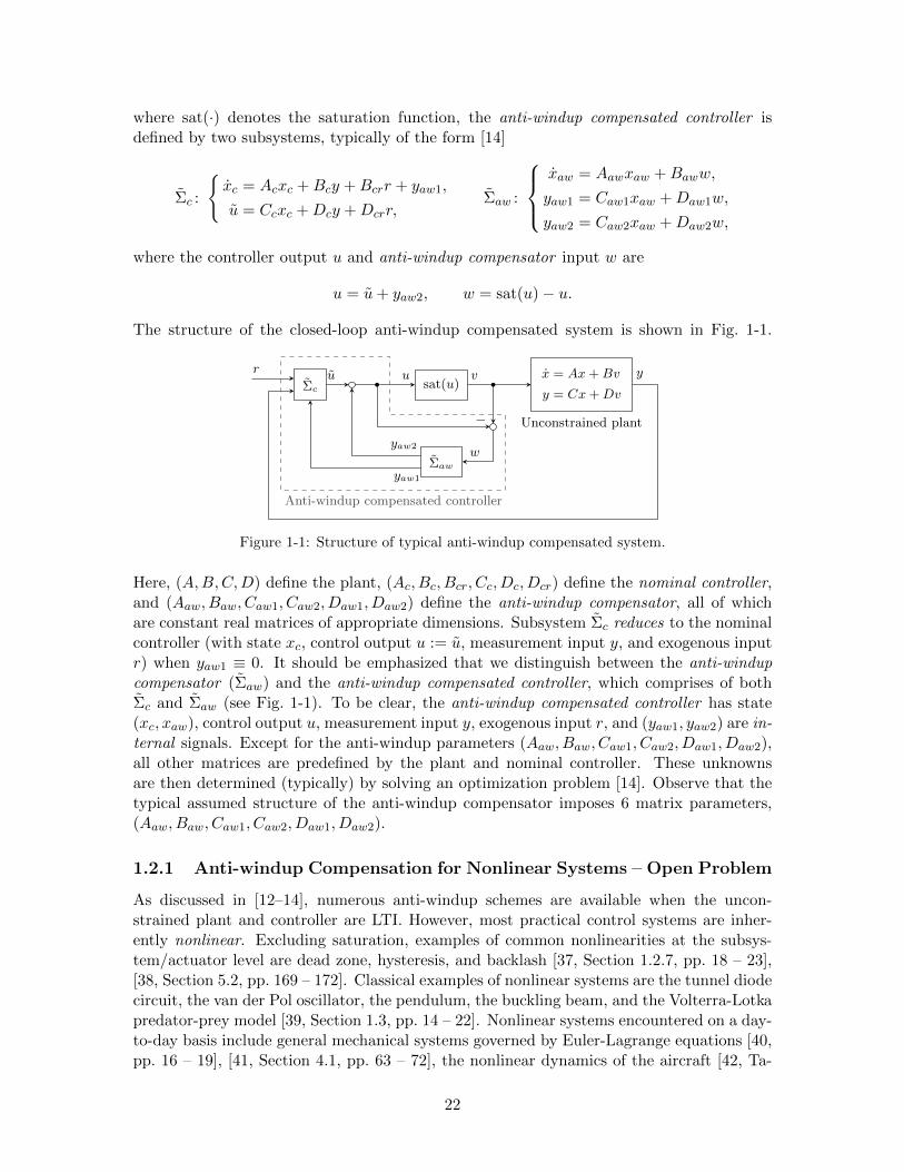
The structure of the closed-loop anti-windup compensated system is shown in Fig. 1-1.

sat(u)x = Ax+Bv

y = Cx+Dv

Unconstrained plant

Σc

Σaw

r u u v

−

w

yaw1

yaw2

y

Anti-windup compensated controller

Figure 1-1: Structure of typical anti-windup compensated system.

Here, (A,B,C,D) define the plant, (Ac, Bc, Bcr, Cc, Dc, Dcr) define the nominal controller,and (Aaw, Baw, Caw1, Caw2, Daw1, Daw2) define the anti-windup compensator, all of whichare constant real matrices of appropriate dimensions. Subsystem Σc reduces to the nominalcontroller (with state xc, control output u := u, measurement input y, and exogenous inputr) when yaw1 ≡ 0. It should be emphasized that we distinguish between the anti-windupcompensator (Σaw) and the anti-windup compensated controller, which comprises of bothΣc and Σaw (see Fig. 1-1). To be clear, the anti-windup compensated controller has state(xc, xaw), control output u, measurement input y, exogenous input r, and (yaw1, yaw2) are in-ternal signals. Except for the anti-windup parameters (Aaw, Baw, Caw1, Caw2, Daw1, Daw2),all other matrices are predefined by the plant and nominal controller. These unknownsare then determined (typically) by solving an optimization problem [14]. Observe that thetypical assumed structure of the anti-windup compensator imposes 6 matrix parameters,(Aaw, Baw, Caw1, Caw2, Daw1, Daw2).

1.2.1 Anti-windup Compensation for Nonlinear Systems – Open Problem

As discussed in [12–14], numerous anti-windup schemes are available when the uncon-strained plant and controller are LTI. However, most practical control systems are inher-ently nonlinear. Excluding saturation, examples of common nonlinearities at the subsys-tem/actuator level are dead zone, hysteresis, and backlash [37, Section 1.2.7, pp. 18 – 23],[38, Section 5.2, pp. 169 – 172]. Classical examples of nonlinear systems are the tunnel diodecircuit, the van der Pol oscillator, the pendulum, the buckling beam, and the Volterra-Lotkapredator-prey model [39, Section 1.3, pp. 14 – 22]. Nonlinear systems encountered on a day-to-day basis include general mechanical systems governed by Euler-Lagrange equations [40,pp. 16 – 19], [41, Section 4.1, pp. 63 – 72], the nonlinear dynamics of the aircraft [42, Ta-

22

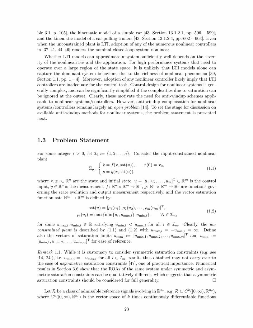
ble 3.1, p. 105], the kinematic model of a simple car [43, Section 13.1.2.1, pp. 596 – 599],and the kinematic model of a car pulling trailers [43, Section 13.1.2.4, pp. 602 – 603]. Evenwhen the unconstrained plant is LTI, adoption of any of the numerous nonlinear controllersin [37–41, 44–46] renders the nominal closed-loop system nonlinear.

Whether LTI models can approximate a system sufficiently well depends on the sever-ity of the nonlinearities and the application. For high performance systems that need tooperate over a large region of the state space, it is unlikely that LTI models alone cancapture the dominant system behaviors, due to the richness of nonlinear phenomena [39,Section 1.1, pp. 1 – 4]. Moreover, adoption of any nonlinear controller likely imply that LTIcontrollers are inadequate for the control task. Control design for nonlinear systems is gen-erally complex, and can be significantly simplified if the complexities due to saturation canbe ignored at the outset. Clearly, these motivate the need for anti-windup schemes appli-cable to nonlinear systems/controllers. However, anti-windup compensation for nonlinearsystems/controllers remains largely an open problem [14]. To set the stage for discussion onavailable anti-windup methods for nonlinear systems, the problem statement is presentednext.

1.3 Problem Statement

For some integer i > 0, let Ii := 1, 2, . . . , i. Consider the input-constrained nonlinearplant

Σp :

x = f(x, sat(u)), x(0) = x0,

y = g(x, sat(u)),(1.1)

where x, x0 ∈ Rn are the state and initial state, u = [u1, u2, . . . , um]T ∈ Rm is the controlinput, y ∈ Rp is the measurement, f : Rn×Rm → Rn, g : Rn×Rm → Rp are functions gov-erning the state evolution and output measurement respectively, and the vector saturationfunction sat : Rm → Rm is defined by

sat(u) = [ρ1(u1), ρ2(u2), . . . , ρm(um)]T,

ρi(ui) = maxminui, umax,i, umin,i, ∀i ∈ Im,(1.2)

for some umax,i, umin,i ∈ R satisfying umin,i < umax,i for all i ∈ Im. Clearly, the un-constrained plant is described by (1.1) and (1.2) with umax,i = −umin,i = ∞. Definealso the vectors of saturation limits umax := [umax,1, umax,2, . . . , umax,m]T and umin :=[umin,1, umin,2, . . . , umin,m]T for ease of reference.

Remark 1.1. While it is customary to consider symmetric saturation constraints (e.g. see[14, 24]), i.e. umin,i = −umax,i for all i ∈ Im, results thus obtained may not carry over tothe case of asymmetric saturation constraints [47], one of practical importance. Numericalresults in Section 3.6 show that the ROAs of the same system under symmetric and asym-metric saturation constraints can be qualitatively different, which suggests that asymmetricsaturation constraints should be considered for full generality.

LetR be a class of admissible reference signals evolving in Rnr , e.g.R ⊂ Ck([0,∞),Rnr),where Ck([0,∞),Rnr) is the vector space of k times continuously differentiable functions

23

[0,∞)→ Rnr . For any reference input r ∈ R, let the nominal controller be described by

Σc :

xc = fc(xc, y, r), xc(0) = xc0,

uc = gc(xc, y, r),(1.3)

where xc, xc0 ∈ Rq are the state and initial state, uc ∈ Rm is the controller output, y ∈ Rpis the measurement input, and fc : Rq×Rp×Rnr → Rq, gc : Rq×Rp×Rnr → Rm govern thecontroller state evolution and output. Assume that the nominal controller (1.3) has beendesigned such that the uncompensated closed-loop system (also called the uncompensatedsystem or the nominal system) defined by (1.1), (1.2), (1.3), and the relation u ≡ uc iswell-posed, and achieves some nominal stability and performance.

Remark 1.2. Clearly, r(t) ∈ Rnr means the instantaneous value of the function r ∈ R,r : [0,∞)→ Rnr , at time t. By an abuse of notation, we will also use r (:= r(t)) to denotethe same instantaneous value of the function r ∈ R, the meaning of which should be clearfrom context. Observe that r in (1.3) refers to the instantaneous function value.

Remark 1.3. While we recognize the importance of robustness issues associated with thepresence of noise, disturbances, time delays, and unmodeled dynamics in any control system,it appears superfluous at this point to consider these, given that the topic is still largelyan open problem [14]. We leave the study of these (important) issues as future work (seeSection 7.1.1).

Problem 1 (Anti-windup Compensation for Nonlinear Systems). The goal is to design ananti-windup compensated controller (see Section 1.2)

Σaw :

xaw = faw(xaw, y, r), xaw(0) = xaw0,

uaw = gaw(xaw, y, r),(1.4)

with state xaw ∈ Rq, inputs (y, r) and m dimensional output uaw ∈ Rm, and determine astate initialization xaw0, such that the anti-windup compensated system defined by (1.1),(1.2), (1.4), and the relation u ≡ uaw satisfy:

(i) when (r, x0, xc0) ∈ R×Rn×Rq are such that the uncompensated system remains stable,then the anti-windup compensated system must also remain stable for (r, x0, xaw0) ∈R× Rn × Rq;

(ii) for every (r, x0, xc0) such that the controls never saturate for the uncompensatedsystem, i.e. sat(uc) ≡ uc, the control signal of the anti-windup compensated systemfor (r, x0, xaw0) satisfies uaw ≡ uc;

(iii) when (r, x0, xc0) are such that some controls saturate for the uncompensated system(i.e. there exists a non-trivial interval [t1, t2], t1 < t2, such that sat(uc(t)) 6= uc(t)for all t ∈ [t1, t2]), then the performance of the anti-windup compensated system for(r, x0, xaw0) must be no worse than the uncompensated system.

Remark 1.4. Examination of the preceding conditions shows that there always exists atrivial solution (Σaw ≡ Σc, xaw0 = xc0) to Problem 1. To exclude the trivial solution, wecan always add a 4th condition:

(iv) there exists (r, x0, xc0) ∈ R × Rn × Rq such that the performance of the anti-windupcompensated system for (r, x0, xaw0) ∈ R×Rn×Rq is strictly better than the uncom-pensated system.

24

We exclude it because it has no real practical significance.

Remark 1.5. Together, conditions (ii) and (iii) means that performance is never reducedwith anti-windup compensation. Hence an equivalent formulation of condition (iii) is:

(iii) for all (r, x0, xc0) ∈ R × Rn × Rq, the performance of the anti-windup compensatedsystem for (r, x0, xaw0) ∈ R × Rn × Rq must be no worse than the uncompensatedsystem.

Remark 1.6. Numerous performance metrics can be specified, depending on the application.A common performance metric is based on L2-gain [14, 48, 49], [41, pp. 18 – 19]. Also,observe that numerous stability criteria can be specified (in particular, see [46, pp. 207 –212]), the suitability of which is again application dependent.

Some observations in the statement of Problem 1:

• Condition (i) states that stability must never be compromised by anti-windup compen-sation. For a regulatory system, i.e. R is a set of constant functions R ⊂ r : [0,∞)→Rnr | ˙r ≡ 0, this condition means that the ROA of the system can only be main-tained/enlarged by anti-windup compensation.• Condition (ii) states that nominal performance is recovered whenever no controls

saturate, a classical requirement. When the nominal controller is a minimal realiza-tion [50], condition (ii) implies that in general, the order of the anti-windup compen-sated controller Σaw must be at least as large as that of the nominal controller Σc,i.e. q ≥ q (see (1.3) and (1.4)).• The requirement for determination of the controller state initialization xaw0 is due

to the recognition that usually, the controller state can be arbitrarily initialized.Such an initialization can be advantageous even if no explicit anti-windup schemeis adopted [51]. Moreover, condition (ii) imply that xaw0 must be dependent on xc0.

1.3.1 Recovering the Anti-windup Compensator

In contrast to the typical anti-windup framework [14], the structure of the anti-windup com-pensated controller is not assumed in Problem 1. This is best seen by comparing Fig. 1-2with Fig. 1-1, where the anti-windup compensated controller Σaw is free to assume anystructure. While this provides much flexibility for the design of the anti-windup compen-

ΣpΣcucr

anti-windup−−−−−−−→ΣpΣaw

uawr

Figure 1-2: Illustration of general anti-windup problem.

sated controller, it may appear that one of the principal advantages of anti-windup schemes,namely their amenability to be retrofitted to an existing controller, is lost. We show herethat an anti-windup compensator can always be obtained from the anti-windup compen-sated controller with either measurement of the nominal controller output, or knowledgeof the nominal controller realization and initial state. Observe that these are reasonablerequirements even to realize the conventional anti-windup compensator Σaw in Fig. 1-1.

Assume that an anti-windup compensated controller Σaw has been designed and is de-scribed by (1.4). When the output of the nominal controller uc in (1.3) can be measured,

25

an additive anti-windup compensator with output uaw can be defined by

Σaw :

xaw = faw(xaw, y, r), xaw(0) = xaw0,

uaw = gaw(xaw, y, r)− uc,(1.5)

so that when the nominal controller’s output uc is added to the derived anti-windup com-pensator’s output uaw, we get the desired control signal u = uc+uaw = gaw(xaw, y, r) = uaw.

Alternatively, if the realization of the nominal controller (1.3) and initial state xc0 areknown, we can incorporate a model of the nominal controller and define the additive anti-windup compensator by

Σaw :

˙xc = fc(xc, y, r), xc(0) = xc0,

xaw = faw(xaw, y, r), xaw(0) = xaw0,

uaw = gaw(xaw, y, r)− gc(xc, y, r).(1.6)

By the preceding construction, we have xc ≡ xc (compare with (1.3)), so that similaraddition yields

u = uc + uaw = uc + gaw(xaw, y, r)− gc(xc, y, r) = uc + gaw(xaw, y, r)− gc(xc, y, r),= uc + gaw(xaw, y, r)− uc = gaw(xaw, y, r) = uaw,

as desired. Fig. 1-3 illustrates the resulting closed-loop system obtained from the derivedadditive anti-windup compensator Σaw. These are two of numerous possible realizations of

ΣpΣc

Σaw

uuc

uaw

r y

Figure 1-3: Closed-loop system with derived anti-windup compensator. The dashed line representsthe case when measurement of uc is available.

anti-windup compensators that can be obtained from the anti-windup compensated control-ler. Each of these realizations comes with its own robustness issues, the study of which weleave as future work (see Section 7.1.2).

1.4 Literature Review

With Problem 1 as objective, we will focus only on literature relevant to anti-windup com-pensation for nonlinear systems, leaving out the vast majority of work on input-constrainedLTI plants driven by LTI controllers [12–14].

1.4.1 Conditioning Technique

One of the early anti-windup schemes is the conditioning technique [51, 52], which is anextension of the back-calculation method reported in [53] (see also [18]). It is importantbecause it forms the conceptual basis for numerous of the methods reviewed in this sec-tion, and it claims to be applicable to controllers of general structure [51]. When some

26

controls saturate, the key idea is to determine a “realizable reference” input rr such thatthe saturation constraints will be satisfied when the true reference5 r is replaced by rr.Conceptually, this newly determined realizable reference is then used, until the point wherethe true reference r causes no saturation constraint violations. The extension to nonlinearsystems is presented in [51], where it was claimed:

“It can be applied to any kind of controller (linear or not, discrete or continu-ous, time varying or not, single-input-single-output or multiple-input-multiple-output).”

While technically correct, the claim may be misleading. The first fundamental difficulty isthat for general controllers of the form (1.3), a system of implicit nonlinear equations ofthe form gc(xc, y, rr) = sat(uc) needs to be solved for rr online. Not only would this becomputationally prohibitive, neither existence nor uniqueness of solutions can be guaranteedin general [54, Section 2.1, pp. 15 – 16]. Moreover, when the nominal controller (1.3) is“strictly proper”, i.e. the output equation has the form uc = gc(xc) and does not depend onr, the conditioning technique breaks down, in the sense that effectively, it yields no anti-windup compensation! This makes the conditioning technique as proposed in [51] ill-suited6

as a candidate method to solve Problem 1.

1.4.2 Feedback Linearizable Nonlinear Systems

The majority of the literature on anti-windup compensation for nonlinear systems appliesto feedback linearizable nonlinear systems [56–66]. Feedback linearization or dynamic in-version [44, Section 4.2, pp. 147 – 161] transforms the input-constrained nonlinear systeminto an equivalent input-constrained LTI system (with state-dependent constraints [56])for which a nominal controller is designed. Then well established anti-windup schemesdeveloped for input-constrained LTI systems are adopted or modified for anti-windup com-pensation. Note that this is a brief oversimplified description, ignoring the complicationsthat arose and were addressed within these papers. These methods are appealing due totheir conceptual simplicity (though by no means trivial), and relates well to establishedtechniques, so insights from the experience on input-constrained LTI systems could be har-nessed to some degree. While these methods are valuable in advancing the state-of-the-art,they are not viable candidates for general nonlinear plants and/or controllers since nonlin-ear systems are not generically feedback linearizable [67, 68], and the nominal controller isrestricted to be a feedback linearizing controller.

1.4.3 Anti-windup Schemes for Particular Controllers

Various anti-windup schemes were proposed in [69–72] for some particular adaptive control-lers, and in [73] for a sliding mode controller [38, Chapter 7, pp. 276 – 306]. These methodsdepend strongly on the underlying structure of the controller, and would not be applicableto general controllers of the form (1.3).

5For consistency in the discussions, we will use the notation established in Section 1.3 whenever possible,instead of notations used in particular papers.

6Note that the restrictions imposed on the nominal controller to avoid some of these limitations are severe(with respect to the nonlinear anti-windup problem), in requiring (i) the output function gc (see (1.3)) tobe linear in r; (ii) the dimensions of reference input and control output to coincide, i.e. nr = m (see thedefinition of r and uc in (1.3)). See also [55] for a criticism of the conditioning technique when applied toinput-constrained LTI systems.

27

1.4.4 Nonlinear Anti-windup for Euler-Lagrange Systems

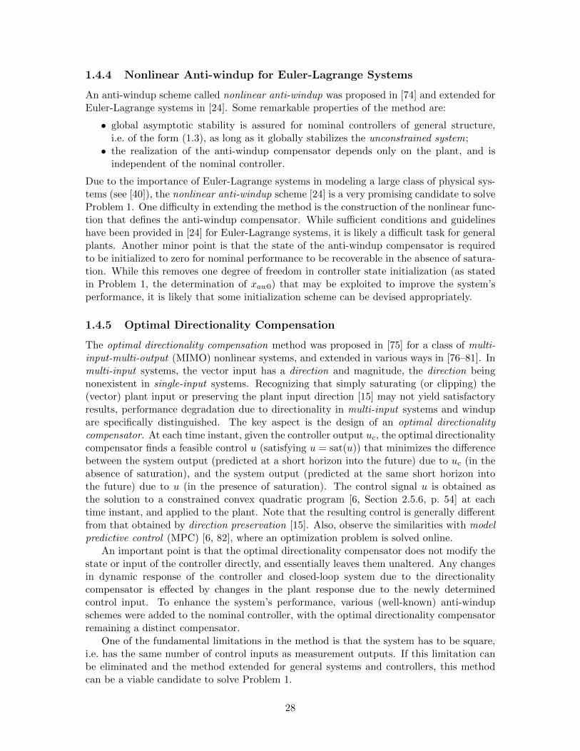
An anti-windup scheme called nonlinear anti-windup was proposed in [74] and extended forEuler-Lagrange systems in [24]. Some remarkable properties of the method are:

• global asymptotic stability is assured for nominal controllers of general structure,i.e. of the form (1.3), as long as it globally stabilizes the unconstrained system;• the realization of the anti-windup compensator depends only on the plant, and is

independent of the nominal controller.

Due to the importance of Euler-Lagrange systems in modeling a large class of physical sys-tems (see [40]), the nonlinear anti-windup scheme [24] is a very promising candidate to solveProblem 1. One difficulty in extending the method is the construction of the nonlinear func-tion that defines the anti-windup compensator. While sufficient conditions and guidelineshave been provided in [24] for Euler-Lagrange systems, it is likely a difficult task for generalplants. Another minor point is that the state of the anti-windup compensator is requiredto be initialized to zero for nominal performance to be recoverable in the absence of satura-tion. While this removes one degree of freedom in controller state initialization (as statedin Problem 1, the determination of xaw0) that may be exploited to improve the system’sperformance, it is likely that some initialization scheme can be devised appropriately.

1.4.5 Optimal Directionality Compensation

The optimal directionality compensation method was proposed in [75] for a class of multi-input-multi-output (MIMO) nonlinear systems, and extended in various ways in [76–81]. Inmulti-input systems, the vector input has a direction and magnitude, the direction beingnonexistent in single-input systems. Recognizing that simply saturating (or clipping) the(vector) plant input or preserving the plant input direction [15] may not yield satisfactoryresults, performance degradation due to directionality in multi-input systems and windupare specifically distinguished. The key aspect is the design of an optimal directionalitycompensator. At each time instant, given the controller output uc, the optimal directionalitycompensator finds a feasible control u (satisfying u = sat(u)) that minimizes the differencebetween the system output (predicted at a short horizon into the future) due to uc (in theabsence of saturation), and the system output (predicted at the same short horizon intothe future) due to u (in the presence of saturation). The control signal u is obtained asthe solution to a constrained convex quadratic program [6, Section 2.5.6, p. 54] at eachtime instant, and applied to the plant. Note that the resulting control is generally differentfrom that obtained by direction preservation [15]. Also, observe the similarities with modelpredictive control (MPC) [6, 82], where an optimization problem is solved online.

An important point is that the optimal directionality compensator does not modify thestate or input of the controller directly, and essentially leaves them unaltered. Any changesin dynamic response of the controller and closed-loop system due to the directionalitycompensator is effected by changes in the plant response due to the newly determinedcontrol input. To enhance the system’s performance, various (well-known) anti-windupschemes were added to the nominal controller, with the optimal directionality compensatorremaining a distinct compensator.

One of the fundamental limitations in the method is that the system has to be square,i.e. has the same number of control inputs as measurement outputs. If this limitation canbe eliminated and the method extended for general systems and controllers, this methodcan be a viable candidate to solve Problem 1.

28

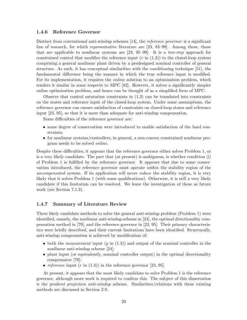
1.4.6 Reference Governor

Distinct from conventional anti-windup schemes [14], the reference governor is a significantline of research, for which representative literature are [23, 83–99]. Among these, thosethat are applicable to nonlinear systems are [23, 95–99]. It is a two-step approach forconstrained control that modifies the reference input (r in (1.3)) to the closed-loop systemcomprising a general nonlinear plant driven by a predesigned nominal controller of generalstructure. As such, it has conceptual similarities with the conditioning technique [51], thefundamental difference being the manner in which the true reference input is modified.For its implementation, it requires the online solution to an optimization problem, whichrenders it similar in some respects to MPC [82]. However, it solves a significantly simpleronline optimization problem, and hence can be thought of as a simplified form of MPC.

Observe that control saturation constraints in (1.3) can be translated into constraintson the states and reference input of the closed-loop system. Under some assumptions, thereference governor can ensure satisfaction of constraints on closed-loop states and referenceinput [23, 95], so that it is more than adequate for anti-windup compensation.

Some difficulties of the reference governor are:

• some degree of conservatism were introduced to enable satisfaction of the hard con-straints;• for nonlinear systems/controllers, in general, a non-convex constrained nonlinear pro-

gram needs to be solved online.

Despite these difficulties, it appears that the reference governor either solves Problem 1, oris a very likely candidate. The part that (at present) is ambiguous, is whether condition (i)of Problem 1 is fulfilled by the reference governor. It appears that due to some conser-vatism introduced, the reference governor must operate within the stability region of theuncompensated system. If its application will never reduce the stability region, it is verylikely that it solves Problem 1 (with some qualifications). Otherwise, it is still a very likelycandidate if this limitation can be resolved. We leave the investigation of these as futurework (see Section 7.1.3).

1.4.7 Summary of Literature Review

Three likely candidate methods to solve the general anti-windup problem (Problem 1) wereidentified, namely, the nonlinear anti-windup scheme in [24], the optimal directionality com-pensation method in [79], and the reference governor in [23, 95]. Their primary characteris-tics were briefly described, and their current limitations have been identified. Structurally,anti-windup compensation is achieved by modification of:

• both the measurement input (y in (1.3)) and output of the nominal controller in thenonlinear anti-windup scheme [24];• plant input (or equivalently, nominal controller output) in the optimal directionality

compensator [79];• reference input (r in (1.3)) in the reference governor [23, 95].

At present, it appears that the most likely candidate to solve Problem 1 is the referencegovernor, although more work is required to confirm this. The subject of this dissertationis the gradient projection anti-windup scheme. Similarities/relations with these existingmethods are discussed in Section 2.9.

29

1.5 Dissertation Overview

The remainder of this dissertation is briefly described below.

Chapter 2 – Construction and Fundamental Properties

As mentioned previously, the subject of this dissertation is the gradient projection anti-windup (GPAW) scheme, constructed for general saturated nonlinear plants driven by non-linear controllers. In Chapter 2, we construct the GPAW-compensated controller and showthat it is a generalization of the well-known conditional integration method for PID-typecontrollers [53], [17, Section 3.3.2, p. 38]. This generalization depends critically on the pro-jection operator that in turn is obtained by extension of Rosen’s gradient projection methodfor nonlinear programming [100, 101] to continuous time. Fundamental properties like thecontroller state-output consistency property of GPAW-compensated controllers, as well aspassivity and L2-gain of the projection operator are established. The pertinent featuresof the GPAW scheme are demonstrated on a two-link robot driven by an adaptive slidingmode controller [102].

Chapter 3 – Input Constrained Planar LTI Systems

In Chapter 3, we study the simplest possible saturated feedback system, namely an input-constrained first order LTI plant driven by a first order LTI controller, where the objectiveis to regulate the system state about the origin. For this simple system, strong results onGPAW compensation are obtained, the most notable of which is that GPAW compensation(which reduces to the conditional integration method) can only maintain/enlarge the ROAof the uncompensated system. Qualitative weaknesses of some results in existing anti-windup literature are illustrated, which motivates a new paradigm to address the anti-windup problem, reflected in the statement of Problem 1 in Section 1.3. Numerical resultsin this chapter also imply that asymmetric saturation constraints should be considered forgeneral input-constrained systems.

Chapter 4 – Geometric Properties and Region of Attraction Comparison Results

The main themes of Chapter 4 are geometric properties of GPAW-compensated systems andsome ROA comparison results. Despite being primarily defined by a combinatorial opti-mization subproblem, we show that the GPAW-compensated controller can be equivalentlydefined by the online solution to either a convex quadratic program or a projection ontoa convex polyhedral cone problem. This is significant because it allows a computationallyattractive realization, and holds regardless of the nonlinearities in the plant or nominalcontroller. A geometric bounding condition that relates the vector fields of the nominal andGPAW-compensated controller is presented. Motivated by results in Chapter 3, ROA com-parison results consistent with the new anti-windup paradigm are presented. The chapterends with demonstrations of these ROA comparison results on some simple systems.

Chapter 5 – Input Constrained MIMO LTI Systems

Clearly, LTI models are widely used to approximate practical control systems. SaturatedMIMO LTI plants driven by MIMO LTI controllers are studied in Chapter 5. An ROA

30

comparison result of Chapter 4 is specialized to yield a stability result, which can be veri-fied by solving an LMI problem. We show how the familiar similarity transformation canbe applied to GPAW-compensated controllers, and that under some choice of the GPAWparameter, the GPAW-compensated system can be transformed into a linear system withpartial state constraints, which has been studied in [103–106]. This link allows existingstability results to be applied to this class of GPAW-compensated systems, and vice versa.

Chapter 6 – Numerical Comparisons

In Chapter 6, we compare the GPAW scheme against two anti-windup schemes for nonlinearsystems, and an anti-windup scheme for LTI systems, using some non-trivial examplesavailable in the literature. Thus far, the stability results obtained in Chapters 4 and 5 are tooconservative to be applied to these examples. Nevertheless, we show that even in the absenceof stability results, ad hoc methods can be devised to determine the GPAW parameter suchthat the GPAW-compensated system achieves qualitatively similar performance as thesestate-of-the-art anti-windup schemes. These show that even in the absence of stabilityproofs, the GPAW scheme can be a viable candidate anti-windup method when no otheranti-windup schemes are suitable.

Chapter 7 – Conclusions and Future Work

In Chapter 7, we summarize the main results and present possible areas for future research.This dissertation represents the first steps in the study of GPAW compensation, which hasmuch potential to be developed into a formidable tool to address the problems caused bycontrol saturation. Some possible links with other fields of controls and dynamical systemsare identified, which may provide fruitful research on a theoretical as well as practical level.

Appendix A – Closed Form Expressions for Single-output GPAW-CompensatedControllers

Appendix A presents closed-form expressions for single-output GPAW-compensated control-lers, which includes the case when the nominal controller is of PID-type. These closed-formexpressions allow a computationally efficient implementation of the GPAW-compensatedcontroller.

Appendix B – Closed Form Expressions for GPAW-Compensated Controllerswith Output of Dimension Two

Appendix B presents closed-form expressions for GPAW-compensated controllers with out-put of dimension two. Computational results show that using these closed-form expressionsrequires on average less than 10% of computation power compared to the best case quadraticprogram realization of GPAW-compensated controllers.

Appendix C – Procedure to Apply GPAW Compensation

There are three equivalent ways to realize general GPAW-compensated controllers, detailedin different sections of this dissertation. For ease of reference, we summarize the procedureto apply GPAW compensation in Appendix C.

31

1.6 Contributions

Contributions of the research presented herein are listed below.

• Developed General Purpose Anti-windup Scheme. The GPAW scheme isa general purpose anti-windup scheme constructed for saturated nonlinear systemsdriven by output-feedback nonlinear controllers, and can be easily specialized as ap-propriate. It has clear geometric properties and is characterized by a passive projectionoperator with L2-gain less than one. It achieves controller state-output consistency, aproperty unique to GPAW-compensated controllers, while being an implicit objectivefor most anti-windup schemes.

• Motivated a New Paradigm for Anti-windup Problems. We demonstratedthe qualitative weaknesses of some existing results in the anti-windup literature, whichmotivated a new paradigm to address the anti-windup problem. This new paradigmis to search for results relative to the uncompensated system, such that it will giveclear indications of benefits gained by adopting the anti-windup scheme.

• Demonstrated Need to Consider Asymmetric Saturation Constraints forGeneral Saturated Systems. Numerical results showed that even for a simplesaturated system, the ROAs induced by symmetric and asymmetric saturation con-straints are fundamentally different. ROAs induced by symmetric saturation con-straints are invalid when the saturation constraints become asymmetric, even whenthey are relaxed. This applies to general saturated systems and shows the need toconsider the asymmetric case. We note that the majority of literature on saturatedsystems considers only the symmetric saturation case, and GPAW compensation ap-plies whether the saturation constraints are symmetric or otherwise.

• Developed ROA Comparison and Stability Results for GPAW-CompensatedSystems. Consistent with the new paradigm to search for results relative to the un-compensated system, the ROA comparison results are the first steps in this direction.These results are applicable to fairly general nonlinear systems and controllers, al-though they are likely conservative.

• Demonstrated Viability of GPAW Scheme as a Candidate Anti-windupScheme for General Systems. The GPAW scheme was constructed for generalnonlinear systems and controllers. Even when current stability results are too conser-vative to be applicable, we show that ad hoc methods can be devised to design theGPAW-compensated controller to yield (numerically) satisfactory solutions. This willappeal to practitioners in need of a candidate anti-windup scheme when otherwise,no suitable candidates exist.

• Related GPAW-Compensated Systems to Projected Dynamical Systemsand Linear Systems with Partial State Constraints. For the constrainedplanar LTI system, we showed that it is in fact a projected dynamical system [107–110]. For constrained MIMO LTI systems, we established a link with linear systemswith partial state constraints [103–106]. These links with existing research are strategicin nature, and will motivate much research that may allow cross utilization of ideasand methods in seemingly unrelated fields.

32

Chapter 2

Construction and FundamentalProperties

The subject of this dissertation is the gradient projection anti-windup (GPAW) scheme.In this chapter, we present the GPAW scheme by constructing the GPAW-compensatedcontroller, together with some of its fundamental properties. The GPAW scheme is a gener-alization of the well known conditional integration method, which is described in Section 2.1.The extension of the conditional integration method to MIMO nonlinear systems requiresthe projection operator (Section 2.4), which is derived from the extension of the well-knowngradient projection method for nonlinear programming (Section 2.2) to continuous time(Section 2.3). Using the projection operator, we construct the GPAW-compensated con-troller in Section 2.5. It is shown that under a mild restriction on the structure of thenominal controller, the projection operator enables the GPAW-compensated controller toachieve controller state-output consistency, a unique property among existing anti-windupschemes. In Section 2.6, we show how nominal controllers of general structure can be ap-proximated arbitrarily well to have the required structure, so that GPAW compensationcan be applied to the approximate controller yielding the same desirable properties. InSection 2.7, the projection operator is shown to be passive and with L2-gain less thanone. Some attractive features of the GPAW scheme are illustrated by a numerical examplein Section 2.8. The chapter ends with a comparison of the GPAW scheme with existinganti-windup schemes in Section 2.9.

2.1 Conditional Integration

Two of the earliest known anti-windup schemes, namely the back-calculation method [17,Section 3.3.3, pp. 38 – 41] and the conditional integration method [17, Section 3.3.2, p. 38],were reported by Fertik and Ross in 1967 [53], 11 years after perhaps the first systematicstudy on the windup phenomenon was published in 1956 [22]. Both of these methodsattempt to achieve controller state-output consistency (see Remark 2.1), by different butclosely related ways (see Remark 2.4). Despite being recognized as perhaps the first paperon anti-windup compensation [12, 14], the methods reported in [53] should have been well-known among practitioners in varied forms, as evidenced by the numerous patents [16, 111–117] filed1 prior to 1967. While the back-calculation method has been extended in various

1The patents [16, 111–117] are interesting, and provide a glimpse of the problems faced by the earlycontrollers, as well as some early industrial solutions that were adopted to mitigate those problems. The

33

ways (e.g. to yield the conditioning technique, see Section 1.4.1) and continues to formthe conceptual basis for numerous modern anti-windup schemes, much less effort has beendevoted to the extension of the conditional integration method.2 As will be seen, the GPAWscheme is in fact the natural extension of the conditional integration method reported byFertik and Ross [53] for MIMO nonlinear controllers.

Remark 2.1. Controller state-output consistency is achieved when the controller outputsatisfies the saturation constraints inherently without additional limiting of the output,i.e. sat(uc) = uc. For the controller (1.3), this is achieved when (xc, y, r) are such thatsat(gc(xc, y, r)) = gc(xc, y, r). Observe that this can be achieved by either modificationof xc, y, or r. The conditioning technique (see Section 1.4.1) and reference governor (seeSection 1.4.6) introduce a variable rr in place of r to achieve this, then attempts to drive rrtowards r. The standard anti-windup compensator (see Fig. 1-1) modifies the measurementy (i.e. introduce variable yr and attempt to drive yr towards y), and/or xc through xc,and/or output uc. The GPAW scheme only modifies xc through its evolution, xc.

Consider the description of the conditional integration method (called “accumulatortechnique” in [53]) by Fertik and Ross:

“The overshoot problem discussed above for the accumulation method may beovercome (when velocity-limited) by ignoring the excess integral action when itis the same sign as the desired output.”

For the PID controller described by

ei = e,

u = Kpe+Kiei +Kde,

with saturation constraints umin ≤ u ≤ umax, umin < 0 < umax, this translates into the

back-calculation method was described for analog controllers in [16] (filed on May 18, 1961), which was alsoused for bumpless transfer [12] among multiple analog controllers. One form of conditional integration wasdescribed for analog controllers in [111] (filed on May 26, 1961). A form of conditional integration closestto the method proposed by Fertik and Ross in [53] was described for digital controllers in [114] (filed onJan. 17, 1966):

“A proportional gain channel operates to provide a term in accordance with the proportionalgain constant and the error signal. The proportional term and the integral term are combinedin the output register. The digital count in the output register is used to control the actuatorthrough a digital to analog converter. The output register includes means for establishlishing[sic] limit conditions. These limit conditions are sensed, and in the event that the count is suchthat the controlled device is either fully opened or closed, the multi-rate sampler is inhibitedduring each scan, preventing accumulation of additional error pulses in the integral term untilsuch time as control is again achieved.”

Observe also that Charles W. Ross, co-author of [53], is also a co-inventor of patent [117] (filed on Mar. 14,1968).

2The apparent lack of interest to extend the conditional integration method could be due to historical ortechnical reasons. We first note that the focus of [53] is the back-calculation method, while the conditionalintegration method is only mentioned in passing, described by only a single sentence quoted on this page.Early successes of anti-windup schemes derived from the back-calculation method, like the conditioning tech-nique, could have diverted attention away from the less-proven conditional integration method. Moreover,the conditional integration method induces a switched or hybrid closed-loop system [118, 119] describedby a differential equation with discontinuous right-hand side [120] (see Section 3.2). These topics beingpoorly understood in the early development of anti-windup schemes could be another reason for the lack ofextensions of the conditional integration method.

34

anti-windup compensated controller3

ei =

0, if ((u ≥ umax) ∨ (u ≤ umin)) ∧ (eu > 0),

e, otherwise,

u = Kpe+Kiei +Kde,

where A ∨B means “A OR B” and A ∧B means “A AND B” for logical statements A, Bthat evaluates to true or false. This can be rewritten as

ei =

0, if (u ≥ umax) ∧ (e > 0),

0, if (u ≤ umin) ∧ (e < 0),

e, otherwise,

u = Kpe+Kiei +Kde.

(2.1)

As can be seen, the fundamental idea is simple, intuitive, and elegant. It simply stopsintegrating only when such integration will cause the term Kiei to increase/decrease in amanner to aggravate the existing saturation constraint violation.

Remark 2.2. Observe that the conditional integration method manipulates only the control-ler state (in this case, the integral state) ei through its evolution ei. An equivalent interpre-tation is that it stops integration when the nominal state update will drive ei further awayfrom the unsaturated region K(e, e) = ei ∈ R | sat(Kpe+Kiei+Kde) = Kpe+Kiei+Kde(in this case an interval) under saturation.

Now, consider extending this idea to m decoupled nonlinear controllers, described by

xci = fci(xci, y, r),

uci = gci(xci, y, r),i ∈ Im := 1, 2, . . . ,m,

subject to umin,i ≤ uci ≤ umax,i for all i ∈ Im, where (y, r) are the measurement andreference input respectively. Observe that (uci, xci) do not depend on xcj for all j 6= i, andxci is analogous to the integral state of the PID controller, ei. To apply the same idea (stopintegration whenever it will aggravate saturation constraints) to these decoupled nonlinearcontrollers, we want to achieve xci = 0 when uci ≥ umax,i and the nominal update will drive

the state towards further constraint violations, i.e. when ∂gci∂xci

(xci, y, r)fci(xci, y, r) > 0, andanalogously when uci ≤ umin,i. Then the anti-windup compensated controller is given by

xci =

0, if (uci ≥ umax,i) ∧

( ∂gci∂xci

(xci, y, r)fci(xci, y, r) > 0),

0, if (uci ≤ umin,i) ∧( ∂gci∂xci

(xci, y, r)fci(xci, y, r) < 0),

fci(xci, y, r), otherwise,

uci = gci(xci, y, r),

(2.2)

for all i ∈ Im. It is clear that the preceding also applies to single-output nonlinear control-lers,4 i.e. m = 1.

Remark 2.3. As shown in Appendix A, single-output GPAW-compensated controllers re-

3For the conditional integration to function as intended, we need Ki ≥ 0.4This is not the recommended way to apply GPAW compensation. The GPAW scheme exploits a subtle

but important construction not present here. See Sections 2.5, 2.6, and Appendix C for details.

35

duces to a form similar to (2.2) (compare with the closed-form expressions (A.5)). Thisis expected because the GPAW scheme is a generalization of the conditional integrationmethod.

Now, consider the case for general coupled MIMO nonlinear controllers (1.3),

xc = fc(xc, y, r),

uc = gc(xc, y, r),

where uc = [uc1, uc2, . . . , ucm]T, subject to umin,i ≤ uci ≤ umax,i for all i ∈ Im. In extendingthe same idea, it is clear that we cannot selectively stop the integration of any particularelement of its state xc, since each element will in general affect more than one elementof the controller output. Doing so may adversely affect those controller output elementsthat have not yet reached saturation. Furthermore, stopping integration on all elementsof xc whenever any uci is saturated is far too conservative. What is needed then, at afixed point in time, is a way to update the controller state vector in a manner as close aspossible to the nominal update,5 while attempting not to aggravate any existing saturationconstraints. In other words, at each fixed time, we want to find an f as “close” to fc(xc, y, r)as possible, such that the state evolution governed by xc = f keeps within the unsaturatedregion K(y, r) := x ∈ Rq | gc(x, y, r) = sat(gc(x, y, r)) as much as possible. One way toachieve this is by gradient projection, where we project the nominal update fc(xc, y, r) ontoK(y, r).

Remark 2.4. Both the back-calculation and conditional integration methods attempt toachieve controller state-output consistency. The back-calculation method enforces this re-quirement (possibly by solving a system of nonlinear equations gc(xc, y, r) = sat(uc) forxc, y, or r), while the conditional integration method attempts to achieve this only by notaggravating any existing constraint violations. In this sense, the conditional integrationmethod can be seen as a relaxation of the back-calculation method. Moreover, when theoutput equation is of general structure, i.e. uc = gc(xc, y, r) and

[∂gc∂y ,

∂gc∂r

]6≡ 0 ∈ Rm×(p+nr)

(see (1.3)), it achieves controller state-output consistency only in an approximate sense.6

2.2 Gradient Projection Method for Nonlinear Programming

To extend the conditional integration method to coupled MIMO nonlinear controllers, weneed the gradient projection operator. Here, we describe the gradient projection method fornonlinear programming [100, 101]. It will be extended to continuous time in Section 2.3,after which, the desired operator is “extracted” in Section 2.4.

The gradient projection method [100, 101] solves constrained nonlinear programs of theform7

minx∈Rq

J(x),

subject to h(x) ≤ 0,(2.3)

where x ∈ Rq is the decision variable, J(x) is a possibly nonlinear scalar function J : Rq → R,and h(x) = [h1(x), h2(x), . . . , hk(x)]T is a set of k possibly nonlinear functions h : Rq → Rk.Note that h(x) ≤ 0 is to be interpreted element-wise as k scalar inequalities. In its basic

5Note that this does not mean direction preservation as described in [15].6This is explained in Section 2.5, in particular, Remark 2.13.7Here, we use h instead of h to avoid notational conflicts in Section 2.5.

36

form, the gradient projection method is very powerful, with only very mild differentiabilityrequirements on the functions J and h. However, some additional assumptions like convexityof J and/or h, boundedness of feasible region etc., must be imposed to ensure convergenceto the global minimum [100, 101]. For our purposes, only the projection mechanism is ofinterest, so that analogously, only differentiability of h needs to be assumed.

In the absence of any active constraints, the gradient projection method reduces tothe steepest descent method [100, 101]. The key mechanism that enables the method tomaintain feasibility is gradient projection. Each of the k inequalities hi(x) ≤ 0, i ∈ Ik,defines a hypersurface Gi = x ∈ Rq | hi(x) = 0 ⊂ Rq that forms the boundary of thefeasible region

K = x ∈ Rq | h(x) ≤ 0.On each point x of the boundary of K, each hypersurface Gi that contains x has an asso-ciated supporting hyperplane Hi(x) that is tangent to Gi at x. The normal of Hi at thepoint x is the gradient of hi(x) at x (denoted by ∇hi(x)), which will point “away” from K.These are illustrated in Fig. 2-1.

K

H1

H2

H3 (x

3 )

∇h1 ∇h2

∇h3 (x

3 )G

3

x0

−∇J(x0)

z1x1

−∇J(x1)

z2

zd

x2

−∇J(x2)

z3

x3

−∇J(x3)

Figure 2-1: Visualization of the gradient projection method. K is the feasible region, bounded bythe hypersurfaces H1, H2, and G3. The supporting hyperplane of G3 at x3 is H3(x3).The projection of −∇J(xi) onto Hi yields zi, while zd is the projection of −∇J(x2)onto H1. Notice that to maintain feasibility at x2, it is sufficient to project onto H2. Incontrast, projection onto the intersection of both active constraints corresponding to H1

and H2 will yield the zero vector.

Similar to many optimization methods, the gradient projection method generates asequence xn, the limiting point of which would be the solution to the constrained nonlinearprogram (2.3). Consider now, the case where all hi(x) are affine functions of x [100].Then Gi coincides with Hi, and the boundary of K are all hyperplanes. At a particularpoint xn that lies in the interior of K (cf. x0 in Fig. 2-1), the basic step is taken in adirection to decrease J(xn), i.e. in the negative gradient direction −∇J(xn), much likethe steepest descent method [121, pp. 25 – 26]. When xn lies on the boundary of K(cf. x1, x2, and x3 in Fig. 2-1), the step is taken in a direction “closest” to −∇J(xn) while

37

enforcing xn+1 ∈ K. In this case, if −∇J(xn) points into the interior of K, the nominaldirection is taken. Otherwise, −∇J(xn) is projected onto the intersection of the smallest setof linearly independent hyperplanes Hi that corresponds to active constraints (hi(xn) ≥ 0)that can keep xn+1 within K (cf. z1, z2, and z3 in Fig. 2-1). The step is then taken in thisnew direction, and if some active constraints are nonlinear (cf. G3 in Fig. 2-1), a correctionis added to drive the new point xn+1 back to K [101].

It is important to note that this smallest set of hyperplanes may exclude some activeconstraints, but nonetheless ensures that such exclusion will not cause further constraintviolations. This case is illustrated in Fig. 2-1, at the point x2. Notice here that taking a stepin the direction of −∇J(x2) will violate both constraints corresponding to H1 and H2. Ifwe project onto both of these active constraints, (in other words, the intersection of H1 andH2), the result is the zero vector, and no progress can be made. However, projecting ontoH2 alone, both constraints will be satisfied, and progress can be made in the direction z2.Notice that projecting onto H1 to get zd is ineffective, since taking a step in this directionwill violate the constraint corresponding to H2.

The preceding summarizes the pertinent features of the gradient projection methodrelevant to the GPAW scheme. See [100, 101] for more details, including recursion relationsthat may allow a more computationally efficient implementation.

2.3 Continuous Time Gradient Projection Method

As shown in [122, Appendix B.4, pp. 788 – 791], the continuous time gradient projectionmethod can be obtained by taking the limit as the stepsize of Rosen’s gradient projectionmethod [100, 101] is decreased to zero. The derived continuous time projection operatorhas been used successfully in the context of adaptive control to bound parameter estimatesin some a priori known region in the parameter space [122, Sections 4.4, 8.4.2, and 8.5.5].Another popular projection operator used in adaptive control is presented in [123]. Whileeach has its merits, both of these methods are limited to projection with respect to a singleinequality constraint. Here, we extend Rosen’s gradient projection method [100, 101] tocontinuous time, the principal distinguishing property being its ability to accommodatemultiple inequality constraints.

Recall the constrained nonlinear program (2.3) described by

minx∈Rq

J(x),

subject to h(x) ≤ 0,(2.4)

where x ∈ Rq is the decision variable, J(x) is the scalar objective function J : Rq → R, andh(x) = [h1(x), h2(x), . . . , hk(x)]T is the function h : Rq → Rk defining the k scalar inequalityconstraints. Let Ik := 1, 2, . . . , k be the set of indices corresponding to the k constraintsin problem (2.4), and I ⊂ Ik be some index set of cardinality s := |I| (≤ k). For s > 0,i.e. I 6= ∅, let σI : Is → I be a (non-unique) bijection that assigns an integer in I to eachinteger in Is (= 1, 2, . . . , s). Define the q ×maxs, 1 matrix

NI(x) =

[∇hσI(1)(x),∇hσI(2)(x), . . . ,∇hσI(s)(x)], if s > 0,

0, otherwise,(2.5)

where ∇hi(x) =(∂hi∂x (x)

)T ∈ Rq is the gradient of hi evaluated at the point x ∈ Rq. Observe

38

that when s = 0, i.e. I = ∅, the matrix NI(x) reduces to the zero vector 0 ∈ Rq×1. When0 < s ≤ k, i.e. I 6= ∅, the matrix NI(x) ∈ Rq×s is the concatenation of those gradientvectors ∇hi(x) whose indices are in I, in some order determined by the map σI .

Remark 2.5. Recall that a bijection is a function that establishes a one-to-one correspon-dence between two sets. Note also that any chosen bijection σI : Is → I suffices. Forexample, we can take the ascending order map defined recursively by

σI(i) := min(I \⋃i−1

j=1σI(j)), ∀i ∈ Is.

A different choice of σI only results in a rearrangement of the columns of NI(x). Ourfinal matrix of interest, PI(x) defined below, will be invariant with respect to such re-arrangements (see Remark 2.6). Note that σI is only a construction to allow the indexselection/ordering operations to be stated in a compact mathematical form, it is itself ofno real significance. Indeed, as shown in Appendix A, σI is not needed to construct single-output GPAW-compensated controllers.

For any full rank NI(x), i.e. I 6= ∅ and rank(NI(x)) = mins, q = s = |I| (> 0), definethe symmetric q × q projection matrix [100, Theorem 1]

PI(x) =

I −NI(NT

I NI)−1NT

I (x), if I 6= ∅,I, otherwise,

(2.6)

where NI(NTI NI)

−1NTI (x) := NI(x)(NT

I (x)NI(x))−1NTI (x). Since rank(NT

I NI(x)) =rank(NI(x)) [124, p. 13], whenever NI(x) is full rank, the s×s inverse matrix (NT

I NI(x))−1

exists, and PI(x) is well defined. As shown in [100, Theorem 1], when NI(x) is full rank,PI(x) takes any z ∈ Rq into the orthogonal complement of the subspace spanned by thecolumns of NI(x). In other words, for any x ∈ Rq lying on the constraint boundary andany z ∈ Rq, PI(x)z will be parallel to the intersection of all supporting hyperplanes Hi(x)(see Fig. 2-1) whose indices are in I.

Remark 2.6. Clearly, PI(x) is independent of the bijection σI when I = ∅. To see that PI(x)is invariant with respect to the choice of σI when I 6= ∅, let NI(x) be defined by anotherbijection σI : Is → I, i.e. NI(x) = [∇hσI(1)(x),∇hσI(2)(x), . . . ,∇hσI(s)(x)]. In effect, σIinduces a rearrangement of the columns of NI(x), so that we can write NI(x) = NI(x)Pfor some nonsingular permutation matrix P [124, pp. 25 – 26]. Then when NI(x) is fullrank, we have

NI(NTI NI)

−1NTI (x) = NIP (PTNT

I NIP )−1PTNTI (x) = NI(N

TI NI)

−1NTI (x).

The preceding with (2.6) show that different choices of σI do not alter PI(x).

For any fixed x ∈ Rq, define the sets

Iact := Iact(x) = i ∈ Ik | hi(x) ≥ 0, J := I ⊂ Iact | |I| ≤ q. (2.7)

It can be seen that Iact is the set of indices of all active constraints, and J is the set of allsubsets of Iact with cardinality less than or equal to q. For any fixed x ∈ Rq, define the

39

following combinatorial optimization subproblem

maxI∈J‖PI(x)∇J(x)‖,

subject to rank(NI(x)) = |I|,NTIact(x)PI(x)∇J(x) ≥ 0.

(2.8)

Notice that rank(NI(x)) = |I| holds if and only if either I = ∅ or NI(x) is full rank.Moreover, the condition NT

Iact(x)PI(x)∇J(x) ≥ 0 holds if and only if either x is in the

interior of K = x ∈ Rq | h(x) ≤ 0 (for which Iact = ∅ and NIact = 0 ∈ Rq), or x is onthe boundary of K and −PI(x)∇J(x) points into K from x. Finally, since rank(NI(x)) ≤q for all I ⊂ Iact, J as defined in (2.7) is an exhaustive set of candidate solutions tosubproblem (2.8). In summary, subproblem (2.8) is to find a subset of Iact such thatthe supporting hyperplanes whose indices are in this subset are linearly independent, theprojection of −∇J(x) onto the intersection of these hyperplanes is maximal in magnitude,and when x is evolved in the projection −PI(x)∇J(x), no constraints will be violated. Thefollowing result asserts the existence of solutions to subproblem (2.8).

Proposition 2.3.1 (Existence of Solutions to Combinatorial Optimization Subproblem).For any fixed x ∈ Rq, there exists a solution to subproblem (2.8).

Proof. It is sufficient to show that there always exists a feasible (not necessarily optimal)solution to subproblem (2.8). If v := rank(NIact(x)) = 0 (which includes the case Iact = ∅),then NIact(x) must be a q ×max|Iact|, 1 zero matrix. In this case, it can be verified thatI = ∅ is a feasible solution (in fact, the only feasible solution) to subproblem (2.8).

If v > 0 (necessarily, v ≤ min|Iact|, q), then NIact(x) has exactly v linearly independentcolumns, so that there exists I ⊂ Iact such that rank(NI(x)) = v = |I|, satisfying the firstconstraint of subproblem (2.8). Any column of NIact(x) can then be expressed as a linearcombination of the columns of NI(x), so that NIact(x) = NI(x)Ψ for some Ψ ∈ Rv×|Iact|.From (2.6), we have NT

I (x)PI(x) = 0. Since NTIact(x)PI(x) = ΨTNT

I (x)PI(x) = 0, thesecond constraint of subproblem (2.8) holds, which shows I to be a feasible solution.

Remark 2.7. As noted in the proof of Proposition 2.3.1, NTI (x)PI(x) = 0 for any well

defined PI(x). Note that when I = ∅, we have NTI (x)PI(x) = 0 · I = 0 (see (2.5)

and (2.6)). Writing Iact = (Iact \ I) ∪ I, the second constraint of subproblem (2.8) isequivalent to NT

Iact\I(x)PI(x)∇J(x) ≥ 0 and NTI (x)PI(x)∇J(x) ≥ 0 combined. Since

NTI (x)PI(x)∇J(x) ≡ 0, the second constraint in subproblem (2.8) can be replaced by

NTIact\I(x)PI(x)∇J(x) ≥ 0 without affecting the solution. This yields possibly less condi-

tions to verify (|Iact\I| ≤ |Iact|), and may result in some (marginal) savings in computation.Note that Proposition 2.3.1 can be easily adapted for this variant.

Remark 2.8. It can be verified that for a finite number of constraints k (see (2.4)), there isonly a finite number of candidate solutions given by

|J | =minq,|Iact|∑

i=0

(|Iact|i

)<∞,

where |Iact| ≤ k and(nk

)= n(n−1)...(n−k+1)

k(k−1)...2·1 is the binomial coefficient [125, pp. 824 – 825].

Hence an optimal solution to subproblem (2.8) can always be found by an exhaustive search

40

algorithm, and solvability is not an issue. See Section 4.1 as well as Appendices A and Bfor more properties of the combinatorial optimization subproblem (2.8), and alternativesolution methods.

At each fixed time, let I∗ be a solution to subproblem (2.8). The continuous timegradient projection method is then given by the update

x = −PI∗(x)∇J(x), x(0) = xig,

where xig is the initial guess. Proposition 2.3.1 ensures the existence of I∗, while Remark 2.8shows subproblem 2.8 to be solvable. Together, they show that the continuous time gradientprojection method is well defined.

Our interest in the continuous time gradient projection method lies only in the projectionoperator. As such, we leave the analyses to show that it indeed solves problem (2.4) asfuture work (see Section 7.1.4). The following example demonstrates that the continuoustime gradient projection method can solve a convex nonlinear program. Moreover, whenappropriately initialized, it maintains feasibility at all times.

Example 2.3.1. Consider the convex nonlinear program

minx∈R2

J(x) = xTQ1x,

subject to h1(x) = aT1 x+ b1 ≤ 0,

h2(x) = (x− xcen)TQ2(x− xcen) + b2 ≤ 0,

where

Q1 =

[5 −1−1 5

]> 0, a1 =

[−4−1

], b1 = 4,

Q2 =

[3 22 3

]> 0, xcen =

[22

], b2 = −10.

The feasible region K = x ∈ R2 | h1(x) ≤ 0, h2(x) ≤ 0 is bounded by the line G1 andellipse G2, defined by

G1 = (x1, x2) ∈ R2 | 4x1 + x2 = 4,G2 = x ∈ R2 | (x− xcen)TQ2(x− xcen) + b2 = 0,

and illustrated in Fig. 2-2. It can be verified from [121, Proposition 3.3.2, p. 320] and [121,Proposition 2.1.1, p. 193] that the unique global minimum is x∗ = [1, 1]T.

The solution trajectory of the continuous time gradient projection method is defined by

x = −PI∗(x)∇J(x) = −2PI∗(x)Q1x, x(0) = xig,

where at each fixed time, I∗ is a solution to the combinatorial optimization subproblem

minI∈J‖PI(x)Q1x‖,

subject to rank(NI(x)) = |I|,NTIactPI(x)Q1x ≥ 0,

with Iact, J , PI(x), and NI(x) defined as before.

41

−1 0 1 2 3 4 5 6−1

0

1

2

3

4

5

K

x1

x2

level set contour

global minimum x∗

initial guess xig

trajectory x(t)

boundaries Gi

x∗

Figure 2-2: Continuous time gradient projection method applied to a convex nonlinear program.All solutions starting within the feasible region K converged to the global minimumx∗, maintaining feasibility at all times. Observe that the solution starting from (5, 0),outside the feasible region, also converged to x∗ in this instance.

The simulation results in Fig. 2-2 show that all trajectories considered converged tothe global minimum x∗. It can be seen that the trajectories “slide” along the constraintboundaries when the nominal update would have caused constraint violations. Observethat when started within the feasible region K (xig ∈ (0.2, 4), (2, 2), (4, 1)), feasibility ismaintained at all times, i.e. x(t) ∈ K for all t ≥ 0. Starting from the point xig = (5, 0)outside the feasible region, the solution also converged to the global minimum. Observe thatthe projection mechanism allows solutions to enter, but never to leave the feasible regionK. In general, convergence to the global minimum starting from the infeasible region is notguaranteed. 4

2.3.1 Scaled Continuous Time Gradient Projection Method

Here, we derive a scaled version of the continuous time gradient projection method in similarmanner as in [122, Appendix B.4, pp. 788 – 791]. When the resulting projection operator(see Section 2.4) is used in the GPAW scheme, the scaled variant introduces a parameterthat can be used to tune the GPAW-compensated controller. To obtain the scaled method,define the transformed decision variable x by x = Φx, for some nonsingular scaling matrixΦ ∈ Rq×q. In this new coordinate system, the constrained nonlinear program (2.4) becomes

minx∈Rq

J(Φx),

subject to h(Φx) ≤ 0,(2.9)

with associated gradient vectors and transformed matrix

∇xJ(Φx) :=

(∂J(Φx)

∂x

)T

=

(∂J(Φx)

∂xΦ

)T

= ΦT∇J(Φx), (2.10)

∇xhi(Φx) :=

(∂hi(Φx)

∂x

)T

=

(∂hi(Φx)

∂xΦ

)T

= ΦT∇hi(Φx), ∀i ∈ Ik,

42

NI(Φx) = ΦTNI(Φx). (2.11)

For a full rank NI(Φx), the corresponding projection matrix (obtained from (2.6) by re-placing NI(x) with NI(x) and using (2.11)), is

PI(Φx) =

I − ΦTNI(N

TI ΓNI)

−1NTI (Φx)Φ, if I 6= ∅,

I, otherwise,(2.12)

where Γ := ΦΦT ∈ Rq×q is symmetric positive definite. Written in terms of x, subprob-lem (2.8) becomes

maxI∈J‖PI(x)∇xJ(x)‖,

subject to rank(NI(x)) = |I|,NTIact(x)PI(x)∇xJ(x) ≥ 0,

(2.13)

where we have used rank(NI(x)) = rank(NI(x)).

At each fixed time, let I∗ be a solution to subproblem (2.13). The scaled continuoustime gradient projection method for problem (2.9) is then given by the update

˙x = −PI∗(Φx)∇xJ(Φx), x(0) = Φ−1xig.

Using x = Φx and (2.10), this becomes

x = −ΦPI∗(x)ΦT∇J(x), x(0) = xig, (2.14)

in the original coordinates.

Remark 2.9. The effect of introducing scaling is to perform the projection in the transformedspace. This changes the way the solution evolves on the boundary of the feasible region.

2.4 Projection Operator

Section 2.3 extended Rosen’s gradient projection method [100, 101] to continuous time,while Section 2.3.1 derived a scaled variant. Here, we show that the continuous time gradientprojection method can be separated into two components: a part analogous to the steepestdescent method for optimization, and a projection operator for constraint satisfaction. Theprojection operator is then shown to be applicable to a larger class of constrained problemsgoverned by an ordinary differential equation (ODE).

Using (2.12), we can define

RI(x) := ΦPI(x)Φ−1 =

I − ΓNI(N

TI ΓNI)

−1NTI (x), if I 6= ∅,

I, otherwise,(2.15)

where Γ = ΓT = ΦΦT > 0 is defined in (2.12). The scaled continuous time update (2.14)can then be expressed as

x = −ΦPI∗(x)Φ−1ΦΦT∇J(x) = −RI∗(x)Γ∇J(x), x(0) = xig, (2.16)

where I∗ is a solution to subproblem (2.13).

Observe from (2.7) that when no constraints are active, i.e. Iact = ∅ and J = ∅, the

43

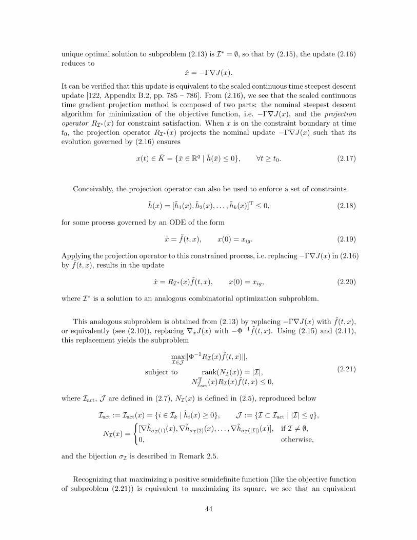
unique optimal solution to subproblem (2.13) is I∗ = ∅, so that by (2.15), the update (2.16)reduces to

x = −Γ∇J(x).

It can be verified that this update is equivalent to the scaled continuous time steepest descentupdate [122, Appendix B.2, pp. 785 – 786]. From (2.16), we see that the scaled continuoustime gradient projection method is composed of two parts: the nominal steepest descentalgorithm for minimization of the objective function, i.e. −Γ∇J(x), and the projectionoperator RI∗(x) for constraint satisfaction. When x is on the constraint boundary at timet0, the projection operator RI∗(x) projects the nominal update −Γ∇J(x) such that itsevolution governed by (2.16) ensures

x(t) ∈ K = x ∈ Rq | h(x) ≤ 0, ∀t ≥ t0. (2.17)

Conceivably, the projection operator can also be used to enforce a set of constraints

h(x) = [h1(x), h2(x), . . . , hk(x)]T ≤ 0, (2.18)

for some process governed by an ODE of the form

x = f(t, x), x(0) = xig. (2.19)

Applying the projection operator to this constrained process, i.e. replacing−Γ∇J(x) in (2.16)by f(t, x), results in the update

x = RI∗(x)f(t, x), x(0) = xig, (2.20)

where I∗ is a solution to an analogous combinatorial optimization subproblem.

This analogous subproblem is obtained from (2.13) by replacing −Γ∇J(x) with f(t, x),or equivalently (see (2.10)), replacing ∇xJ(x) with −Φ−1f(t, x). Using (2.15) and (2.11),this replacement yields the subproblem

maxI∈J‖Φ−1RI(x)f(t, x)‖,

subject to rank(NI(x)) = |I|,NTIact(x)RI(x)f(t, x) ≤ 0,

(2.21)

where Iact, J are defined in (2.7), NI(x) is defined in (2.5), reproduced below

Iact := Iact(x) = i ∈ Ik | hi(x) ≥ 0, J := I ⊂ Iact | |I| ≤ q,

NI(x) =

[∇hσI(1)(x),∇hσI(2)(x), . . . ,∇hσI(|I|)(x)], if I 6= ∅,0, otherwise,

and the bijection σI is described in Remark 2.5.

Recognizing that maximizing a positive semidefinite function (like the objective functionof subproblem (2.21)) is equivalent to maximizing its square, we see that an equivalent

44

subproblem for the definition of I∗ in (2.20) is

maxI∈J

fT(t, x)Γ−1RI(x)f(t, x),

subject to rank(NI(x)) = |I|,NTIact(x)RI(x)f(t, x) ≤ 0,

(2.22)

since from (2.15), we have RTI (x)Γ−1 = Γ−1RI(x) and R2

I(x) = RI(x) (i.e. RI(x) is idem-potent [126, p. 697]), and the square of the objective function of subproblem (2.21) is

‖Φ−1RI(x)f(t, x)‖2 = fT(t, x)RTI (x)Φ−TΦ−1RI(x)f(t, x),

= fT(t, x)RTI (x)Γ−1RI(x)f(t, x),

= fT(t, x)Γ−1R2I(x)f(t, x) = fT(t, x)Γ−1RI(x)f(t, x),

where A−T := (A−1)T = (AT)−1 for any nonsingular matrix A. It can be seen that whenno constraints are active, i.e. Iact = ∅ and J = ∅, the unique optimal solution to sub-problems (2.21) and (2.22) is I∗ = ∅, so that by (2.15), system (2.20) reduces to (2.19).

Remark 2.10. Proposition 2.3.1 as well as Remarks 2.7 and 2.8 apply to subproblems (2.21)and (2.22) with minor changes. Observe that the projection operator has a single parameter,a nonsingular matrix Φ when adopting subproblem (2.21), or a symmetric positive definitematrix Γ when adopting subproblem (2.22).

The following result shows that the projection operator maintains feasibility of theconstraints (2.18) for all future times once the solution of (2.20) enters the feasible regionK. In other words, if there exists a t0 ∈ R such that x(t0) ∈ K, then (2.17) holds.

Proposition 2.4.1 (Feasibility Maintenance Property of Projection Operator). Let x(t) bethe solution of system (2.20), I∗ a solution of either subproblem (2.21) or (2.22). If thereexists a T ∈ R such that h(x(T )) ≤ 0, then h(x(t)) ≤ 0 holds for all t ≥ T .

Proof. Clearly, h(x(t)) = [h1(x(t)), h2(x(t)), . . . , hk(x(t))]T ≤ 0 holds if and only if itselements satisfy hi(x(t)) ≤ 0 for all i ∈ Ik. By assumption, h(x(T )) ≤ 0. It is sufficient

to show that for all i ∈ Ik, whenever hi(x(t)) = 0, then˙hi(x(t)) ≤ 0. Taking the time

derivative yields

˙hi(x(t)) =

∂hi(x(t))

∂xx(t) = ∇hT

i (x(t))RI∗(x(t))f(t, x(t)).

If hi(x(t)) = 0, then i ∈ Iact. Concatenating all gradient vectors with indices in Iact,we need to show that NT

Iact(x(t))RI∗(x(t))f(t, x(t)) ≤ 0. This follows immediately fromthe fact that I∗ is a solution to subproblem (2.21) (or (2.22)), and the second constraintin (2.21) (or (2.22)).

Remark 2.11. An equivalent statement of Proposition 2.4.1 is that K is a positively invariantset [37, p. 127] for the system (2.20).

In summary, the projection operator RI∗(x) is defined by (2.15) and an optimal solutionI∗ to the combinatorial optimization subproblem (2.21) (or equivalently, (2.22)). The pro-jection operator applied to an ODE, i.e. (2.20), maintains feasibility of the constraints (2.18)once the solution enters the feasible region. In the next section, we will use the projectionoperator for anti-windup compensation. Clearly, it can also be used for other purposes,

45

like bounding the parameter estimates of adaptive controllers in some region, as in [122,Sections 4.4, 8.4.2, and 8.5.5]. We leave the exploitation of the projection operator for otherapplications as future work (see Section 7.1.5).

Remark 2.12. Projected dynamical systems (PDS) [107–110] is a significant line of indepen-dent research that has attracted economists, physicists, and mathematicians, among others.It is clear that there is a close relationship between system (2.20) and the PDS. Indeed, itwill be shown in Section 3.2 that the particular GPAW-compensated system considered isin fact a PDS. We leave the investigation of the link in the general case as future work (seeSection 7.1.6).

2.5 Gradient Projection Anti-windup (GPAW) Scheme

In this section, we construct the gradient projection anti-windup (GPAW)-compensatedcontroller using the projection operator developed in Section 2.4. Recall that, classi-cally, windup is interpreted as an inconsistency between the controller state and output,i.e. sat(u) 6≡ u. The GPAW scheme aims to reduce/eliminate this inconsistency, whichcan be achieved if the GPAW controller state can be constrained at all times to lie in theunsaturated region

K(y, r) = x ∈ Rq | sat(gc(x, y, r)) = gc(x, y, r). (2.23)

Proposition 2.4.1 suggests that application of the projection operator on the nominal con-troller may achieve this objective.

Recall the nominal controller (1.3)

xc = fc(xc, y, r), xc(0) = xc0,

uc = gc(xc, y, r).(2.24)

To apply the projection operator on the nominal controller, we make the following identifi-cations between quantities in (2.24) and those in (2.19) and (2.18):

x ∼ xc, xig ∼ xc0, f(t, x) ∼ fc(xc, y, r),

h(x) ∼[

gc(xc, y, r)− umax

−gc(xc, y, r) + umin

], (2.25)

where umax and umin are the vectors of saturation limits defined by the vector saturationfunction (1.2). Notice that the identification of f with fc is motivated by the need to recovernominal performance when no saturation constraints are active, and that (2.25) impliesK = x ∈ Rq | h(x) ≤ 0 ∼ K(y, r). The GPAW-compensated controller8 (see (2.20)and (2.19)) will then be described by

xg = RI∗(xg, y, r)fc(xg, y, r), xg(0) = xc0,

ug = gc(xg, y, r),

where (xg, ug) are the state and output respectively, and RI∗(xg, y, r) remains to be defined.

8See Section 1.2 for a discussion on the distinction between the anti-windup compensator and the anti-windup compensated controller. See also Section 1.3.1 on how to recover an anti-windup compensator froman anti-windup compensated controller.

46

Analogous to the conditional integration method, the GPAW scheme only modifies thecontroller state xg through its evolution xg, and the output equation remains unalteredwith gc defined by the nominal controller (2.24) (see Remark 2.2).

If we were to carry through the steps9 needed to define RI∗(xg, y, r), the GPAW-compensated controller thus obtained (i.e. by applying the projection operator on nomi-nal controllers of the form (2.24)) can achieve controller state-output consistency only inan approximate sense, as corroborated by numerical results in [127]. This is due to thestructure of the output equation ug = gc(xg, y, r) having ug dependent on measurementy and reference input r. For simplicity in the present discussion, restrict consideration tosingle-output controllers, i.e. ug is scalar. Under saturation, i.e. ug = umax or ug = umin,controller state-output consistency requires ug = 0 when the nominal update will aggravatethe existing saturation constraint. The projection operator modifies xg through xg, which,

under these conditions, can be shown10 to induce∂gc(xg ,y,r)

∂xcxg = 0. Hence

ug =∂gc(xg, y, r)

∂xcxg +

∂gc(xg, y, r)

∂yy +

∂gc(xg, y, r)

∂rr =

∂gc(xg, y, r)

∂yy +

∂gc(xg, y, r)

∂rr,

so that in general, ug will be non-zero for arbitrary (y, r). It can also be surmised that theGPAW scheme will be ineffective when∥∥∥∥∂gc(xc, y, r)∂xc

xc

∥∥∥∥ ∥∥∥∥∂gc(xc, y, r)∂yy +

∂gc(xc, y, r)

∂rr

∥∥∥∥ ,holds for the uncompensated controller on the saturation constraint boundaries, since theprojection operator only acts on the controller state.

Remark 2.13. Observe also that the proof of Proposition 2.4.1 breaks down when h doesnot depend on x alone. This would be analogous to the case when gc does not depend onxg alone (for the GPAW-compensated controller).

The preceding discussion motivates us to restrict consideration to “strictly proper”11

nominal controllers of the form

xc = fc(xc, y, r), xc(0) = xc0,

uc = gc(xc),(2.26)

where gc depends only on the controller state xc. Here, as in (2.24), xc, xc0 ∈ Rq arethe controller state and initial state, uc ∈ Rm is the controller output, y ∈ Rp is themeasurement, and r := r(t) ∈ Rnr is the instantaneous reference input.

Remark 2.14. For nominal controllers of the form (2.24), it is shown in Section 2.6 thatan arbitrarily close approximate controller that has the required structure of (2.26) can beconstructed.

As before, we apply the projection operator of Section 2.4 on the nominal control-ler (2.26) by making the following identifications with quantities in (2.19) and (2.18):

x ∼ xc, xig ∼ xc0, f(t, x) ∼ fc(xc, y, r), h(x) ∼[

gc(xc)− umax

−gc(xc) + umin

].

9The construction of RI∗(xg, y, r) will be analogous to the construction of RI∗(x) in Section 2.4.10See the proof of Proposition 2.4.1.11For LTI nominal controllers, observe that this restricts the nominal controllers to have strictly proper

transfer functions.

47

In contrast to (2.25), observe that a crucial difference here is that the last vector definedby gc (being dependent solely on xc) maps directly to h (which depends solely on x).

The resulting GPAW-compensated controller then has the form (see (2.20) and (2.19))

xg = RI∗(xg, y, r)fc(xg, y, r), xg(0) = xc0,

ug = gc(xg),(2.27)

where gc is defined by the nominal controller (2.26) and RI∗(xg, y, r) is to be defined.Observe that apart from the definition of an independent state xg, the only differencewith (2.26) is the introduction of the projection operator RI∗(xg, y, r), which is a state-and-input dependent q × q matrix.

Next, we describe the construction of the projection operator, which is largely analogousto the constructions in Sections 2.3, 2.3.1, and 2.4, made explicit here for clarity. Let gcin (2.27) be decomposed into its m elements, gc = [gc1, gc2, . . . , gcm]T, and define the 2msaturation constraint functions hi by (see (1.2))

hi(xg) = gci(xg)− umax,i,

hi+m(xg) = −gci(xg) + umin,i,∀i ∈ Im := 1, 2, . . . ,m. (2.28)

Observe that hi(xg) ≤ 0 for all i ∈ Im imply sat(gc(xg)) = gc(xg). Assuming differentiabilityof gc, these constraint functions have gradients

∇hi(xg) = ∇gci(xg), ∇hi+m(xg) = −∇gci(xg) = −∇hi(xg), ∀i ∈ Im.

For any index set I ⊂ I2m, define the q ×max|I|, 1 matrix

NI(xg) =

[∇hσI(1)(xg),∇hσI(2)(xg), . . . ,∇hσI(|I|)(xg)], if I 6= ∅,0, otherwise,

(2.29)

where σI : 1, 2, . . . , |I| → I is a chosen (non-unique) bijection (described in Remark 2.5)that assigns an integer in I to each integer in 1, 2, . . . , |I|. For any I ⊂ I2m such thatrank(NI(xg)) = |I|, define the projection matrix RI : Rq → Rq×q

RI(xg) =

I − ΓNI(N

TI ΓNI)

−1NTI (xg), if I 6= ∅,

I, otherwise,(2.30)

where Γ ∈ Rq×q is the single GPAW parameter, chosen to be symmetric positive definite.

Remark 2.15. An attractive feature of the GPAW scheme is that it has only a single sym-metric positive definite matrix parameter, in contrast to the typical anti-windup schemewhich introduced 6 matrix parameters (see Section 1.2). Moreover, observe that multiply-ing a non-zero scalar to Γ does not change RI(xg), so that we can always normalize Γ bysuch scalar multiplications (nominally a positive scalar to preserve positive definiteness).

Define the index set of active saturation constraints, and the candidate solution set

Isat := Isat(xg) = i ∈ I2m | hi(xg) ≥ 0, J := I ⊂ Isat | |I| ≤ q.

48

With (xg, y, r) fixed, the analogue of subproblem (2.22) becomes

maxI∈J

F (I) = fTc (xg, y, r)Γ

−1RI(xg)fc(xg, y, r),

subject to rank(NI(xg)) = |I|,NTIsat(xg)RI(xg)fc(xg, y, r) ≤ 0.

(2.31)

The following result asserts existence of solutions to subproblem (2.31), and is analogous toProposition 2.3.1. While their proofs are similar, we prove it explicitly because the GPAWscheme is the main theme of this dissertation, and to avoid any potential ambiguities causedby notational differences.

Proposition 2.5.1 (Existence of Solutions to Combinatorial Optimization Subproblem).For any fixed (xg, y, r) ∈ Rq × Rp × Rnr , there exists a solution to subproblem (2.31).

Proof. It is sufficient to show that there always exists a feasible (not necessarily optimal)solution to subproblem (2.31). If v := rank(NIsat(xg)) = 0 (which includes the case Isat =∅), then NIsat(xg) must be a q ×max|Isat|, 1 zero matrix. In this case, it can be verifiedthat I = ∅ is a feasible solution (in fact, the only feasible solution) to subproblem (2.31).

If v > 0 (necessarily, v ≤ min|Isat|, q), then NIsat(xg) has exactly v linearly inde-pendent columns, so that there exists I ⊂ Isat such that rank(NI(xg)) = v = |I|, sat-isfying the first constraint of subproblem (2.31). Any column of NIsat(xg) can then beexpressed as a linear combination of the columns of NI(xg), so that NIsat(xg) = NI(xg)Ψfor some Ψ ∈ Rv×|Isat|. From (2.30), we have NT

I (xg)RI(xg) = 0. Since NTIsat(xg)RI(xg) =

ΨTNTI (xg)RI(xg) = 0, the second constraint of subproblem (2.31) holds, which shows I to

be a feasible solution.

Remark 2.16. Observe that Remarks 2.7 and 2.8 apply to subproblem (2.31) with minorchanges. Specifically, for a finite dimensional control output ug ∈ Rm, m < ∞, there canonly be a finite number of candidate solutions, so that an optimal solution to subprob-lem (2.31) can always be found by an exhaustive search algorithm. See Section 4.1, Ap-pendices A and B for more properties of the combinatorial optimization subproblem (2.31),and alternative solution methods.

The next result12 states a property of the objective function of subproblem (2.31) whichfollows immediately from [100, equation (3.20)]. It is useful when deriving closed-formexpressions for the GPAW-compensated controller, as demonstrated in Appendices A and B.

Proposition 2.5.2. If some index set I1 ⊂ Isat is such that rank(NI1(xg)) = |I1|, then the

objective function of subproblem (2.31) satisfies F (I2) ≥ F (I1) for any I2 ⊂ I1.

Proof. Since I2 ⊂ I1, the rank condition rank(NI1(xg)) = |I1| imply rank(NI2(xg)) = |I2|,and ensures that the projection matrices RI1(xg) and RI2(xg) (and hence F (I1) and F (I2))

are well defined. If I1 = I2, then F (I1) = F (I2) and the conclusion holds trivially. AssumeI2 is a strict subset of I1. Since the GPAW parameter Γ ∈ Rq×q is positive definite, it canalways be decomposed as Γ = ΦΦT for some nonsingular Φ ∈ Rq×q [124, Theorem 7.2.7,

12In Proposition 2.5.2, we use accented symbols I1, I2, to avoid confusion with Ii := 1, 2, . . . , i.

49

p. 406]. For any I ⊂ Isat such that rank(NI(xg)) = |I|, define13

PI(xg) := Φ−1RI(xg)Φ =

I − NI(NT

I NI)−1NT

I (xg), if I 6= ∅,I, otherwise,

where NI(xg) := ΦTNI(xg). From its preceding definition, the matrix PI(xg) is a projectionmatrix [100, Theorem 1], and hence satisfies14 [100, equation (3.20)]

‖PI∪j(xg)z‖ ≤ ‖PI(xg)z‖ ≤ ‖z‖, ∀I ⊂ Isat, ∀j ∈ Isat \ I,∀z ∈ Rq. (2.32)

Since Isat is a finite set (due to m < ∞), the set difference I1 \ I2 is also finite. LetI1 \ I2 = i1, i2, . . . , ik, where ij for j ∈ 1, 2, . . . , k (k = |I1| − |I2|) are its elements.Then I1 = I2 ∪ i1 ∪ i2 ∪ · · · ∪ ik. From (2.32), we have

‖PI1(xg)z‖ = ‖PI2∪i1∪···∪ik(xg)z‖ ≤ · · · ≤ ‖PI2∪i1(xg)z‖ ≤ ‖PI2(xg)z‖, ∀z ∈ Rq.

The conclusion F (I2) ≥ F (I1) follows from the preceding by observing that

F (I) = fTc Γ−1RIfc = fT

c Φ−TPIΦ−1fc = fT

c Φ−TPTI PIΦ

−1fc = ‖PIΦ−1fc‖2 = ‖PIz‖2,

where z := Φ−1fc, and the function arguments have been dropped.

Remark 2.17. Proposition 2.5.2 implies that I = ∅ is an optimal solution to subprob-lem (2.31) whenever it is feasible. Since rank(NI(xg)) = |I| always holds for I = ∅, it is anoptimal solution whenever NT

Isat(xg)fc(xg, y, r) ≤ 0. In particular, this happens when noconstraints are active, i.e. Isat = ∅, or when rank(NIsat) = 0, so that NIsat = 0. Observethat when I∗ = ∅, the nominal update is recovered (see (2.27) and (2.30)).

At each fixed time, so that (xg, y, r) is fixed, the GPAW-compensated controller isdefined by (2.27) with RI∗(xg, y, r) defined by (2.30) and a solution I∗ to subproblem (2.31).Note that I∗ depends on (xg, y, r). As mentioned previously, the GPAW scheme aims toachieve controller state-output consistency, which is established in the following theorem.To the best of our knowledge, it is a unique property among anti-windup schemes.15 Thisresult is analogous to Proposition 2.4.1, proven explicitly to avoid ambiguities.

Theorem 2.5.3 (Controller State-output Consistency). Consider the GPAW-compensatedcontroller defined by (2.27), (2.30), and a solution I∗ to subproblem (2.31). If there existsa T ∈ R such that sat(ug(T )) = ug(T ), then sat(ug(t)) = ug(t) holds for all t ≥ T .

Proof. From (1.2), ug = gc(xg) (see (2.27)), and (2.28), it can be seen that sat(ug(t)) = ug(t)holds if and only if hi(xg(t)) ≤ 0 for all i ∈ I2m. By assumption, we have sat(ug(T )) =ug(T ), so that hi(xg(T )) ≤ 0. It is sufficient to show that for all i ∈ I2m, wheneverhi(xg(t)) = 0, then hi(xg(t)) ≤ 0. Taking the time derivative and using (2.27) yields

hi(xg(t)) =∂hi(xg(t))

∂xgxg(t) = ∇hT

i (xg(t))RI∗fc(t, xg(t)),

13This is analogous to PI(x) in (2.15).14This is written using our notation rather than that in [100].15Clearly, specializations of the GPAW scheme (like the conditional integration method) also possess this

property for the same class of nominal controllers. However, note that it must be a true specialization ofthe GPAW scheme. Not all variants of the conditional integration method (e.g. see [17, Section 3.3.2, p. 38])possess this property.

50

where RI∗fc(t, xg(t)) := RI∗(xg(t), y(t), r(t))fc(xg(t), y(t), r(t)). If hi(xg(t)) = 0, theni ∈ Isat. Concatenating all gradient vectors with indices in Isat, we need to show that

NTIsat(xg(t))RI∗fc(t, xg(t)) ≤ 0.

This follows immediately from the fact that I∗ is a solution to subproblem (2.31), and thesecond constraint in (2.31).

Remark 2.18. An equivalent statement of Theorem 2.5.3 is that the unsaturated region

K = x ∈ Rq | sat(gc(x)) = gc(x) = x ∈ Rq | hi(x) ≤ 0,∀i ∈ I2m, (2.33)

is a positively invariant set [37, p. 127] for the solution of the GPAW-compensated con-troller (2.27). Notice that the second equivalent form written in terms of hi follows fromthe observation that sat(gc(xg)) = gc(xg) holds if and only if hi(xg) ≤ 0 for all i ∈ I2m

(see (2.28) and (1.2)).

Remark 2.19. Observe that usually, the controller state can be arbitrarily initialized. If itis initialized such that sat(gc(xc0)) = gc(xc0), Theorem 2.5.3 shows that controller state-output consistency is achieved for all t ≥ 0. Even when the nominal controller’s statecannot be arbitrarily initialized, the same can be achieved by initializing the anti-windupcompensator’s state xaw0 appropriately (see (1.5) and (1.6)).

Remark 2.20. It is clear that we can always impose more controller state constraintshj(xg) ≤ 0, j ∈ 2m+ 1, . . . , 2m+ k. The proof of Theorem 2.5.3 can be readily modifiedto show that these additional constraints will be enforced exactly for all future times oncethey are satisfied at any time instant. If we impose more general constraints of the formhj(xg, x, r) ≤ 0, with (x, r) the plant state and reference input respectively, these constraintswill be satisfied approximately, i.e. not enforced exactly. It can be shown that even withthe introduction of these constraints, those that depend only on the controller state will beenforced exactly by the projection operator. These observations suggest that the projectionoperator may be used for general constrained control [6], with ability to enforce a subset ofconstraints exactly, and others approximately. Indeed, we will demonstrate this by way ofexample in Section 2.8.3.

Theorem 2.5.3 established the controller state-output consistency property of GPAW-compensated controllers when the nominal controller is of the form (2.26), i.e. with gcdepending only on xc. This is a significant result because:

• most anti-windup schemes [12, 14] aim to achieve controller state-output consistency(see Remark 2.21). To the best of our knowledge, this has been achieved only in anapproximate sense to date, whereas the GPAW scheme achieved it exactly ;• it applies to a large class of nonlinear controllers, and is achieved irrespective of the

plant dynamics.16

Remark 2.21. Typically, when a controller is driven by some error signal, the control ob-jective would be achieved exactly if the error signal is identically zero. In most anti-windupschemes, whether the early ad hoc schemes [12] or modern schemes [14], the anti-windupcompensator is driven by the signal (sat(u)−u) (see Fig. 1-1). When controller state-output

16In particular, being independent of plant dynamics implies that GPAW compensation can be applied toadaptive controllers [122] [38, Chapter 8, pp. 311 – 389] without much additional complications.

51

consistency is achieved, i.e. sat(u) ≡ u, this signal would be identically zero. Hence, con-troller state-output consistency is an implicit objective in anti-windup compensators drivenby the signal (sat(u)− u).

One implication of controller state-output consistency is that it allows the saturationfunction to be eliminated in the description of the closed-loop system when the controllerstate is appropriately initialized. The closed-loop system comprising the plant (1.1)

x = f(x, sat(u)), x(0) = x0,

y = g(x, sat(u)),(2.34)

and GPAW-compensated controller (2.27) (with u := ug) can be written as

x = f(x, sat(gc(xg))), x(0) = x0,

xg = RI∗fc(xg, g(x, sat(gc(xg))), r(t)), xg(0) = xc0,(2.35)

where RI∗fc(xg, y, r) := RI∗(xg, y, r)fc(xg, y, r), and we have used r(t) to emphasize thetime-varying nature of the system (see Remark 1.2). When the controller state is initializedsuch that sat(gc(xc0)) = gc(xc0) (see Remark 2.19), the closed-loop system reduces byTheorem 2.5.3 to

x = f(x, gc(xg)), x(0) = x0,

xg = RI∗fc(xg, g(x, gc(xg)), r(t)), xg(0) = xc0,(2.36)

for all t ≥ 0, where the sat(·) function has been eliminated. This shows that all complicationsdue to saturation are accounted for by the projection operator RI∗(xg, y, r). The eliminationof the saturation function in the system description provides significant simplifications whenderiving stability results, examples of which are shown in Sections 4.4 and 5.2.

The effect of applying GPAW compensation is illustrated in Fig. 2-3, which is simi-lar to Fig. 2-1. Here, K is the unsaturated region in the controller state space, xgi :=xg(ti), and fci := fc(xg(ti), y(ti), r(ti)) represents the nominal controller’s vector field attime ti. At each time instant, the combinatorial optimization subproblem (2.31) deter-mines an optimal combination of constraints to project fci, yielding the vector fgi :=RI∗(xg(ti), y(ti), r(ti))fc(xg(ti), y(ti), r(ti)) that defines the GPAW-compensated control-ler. Observe that the unsaturated region K (2.33) does not depend on inputs (y, r), andthe controller state can be constrained within it exactly. For nominal controllers of theform (2.24), the resulting unsaturated region K(y, r) (2.23) varies with inputs (y, r). Inthis case, variations of K(y, r) may cause the controller state to depart it even under pro-jection.

We end this section with some observations:

(i) apart from the restriction on the form of the output function gc of the nominal con-troller, the only assumption needed to construct the projection operator (and hencethe GPAW-compensated controller) is differentiability of gc;

(ii) by construction (see Remark 2.17), the GPAW-compensated controller satisfies con-dition (ii) of Problem 1 (see Section 1.3);

(iii) as shown in Section 3.1 and Appendix A, application of the GPAW scheme to somenominal controllers yields the conditional integration compensated controller. Thisshows that indeed, the GPAW scheme is a generalization of the conditional integrationmethod.

52

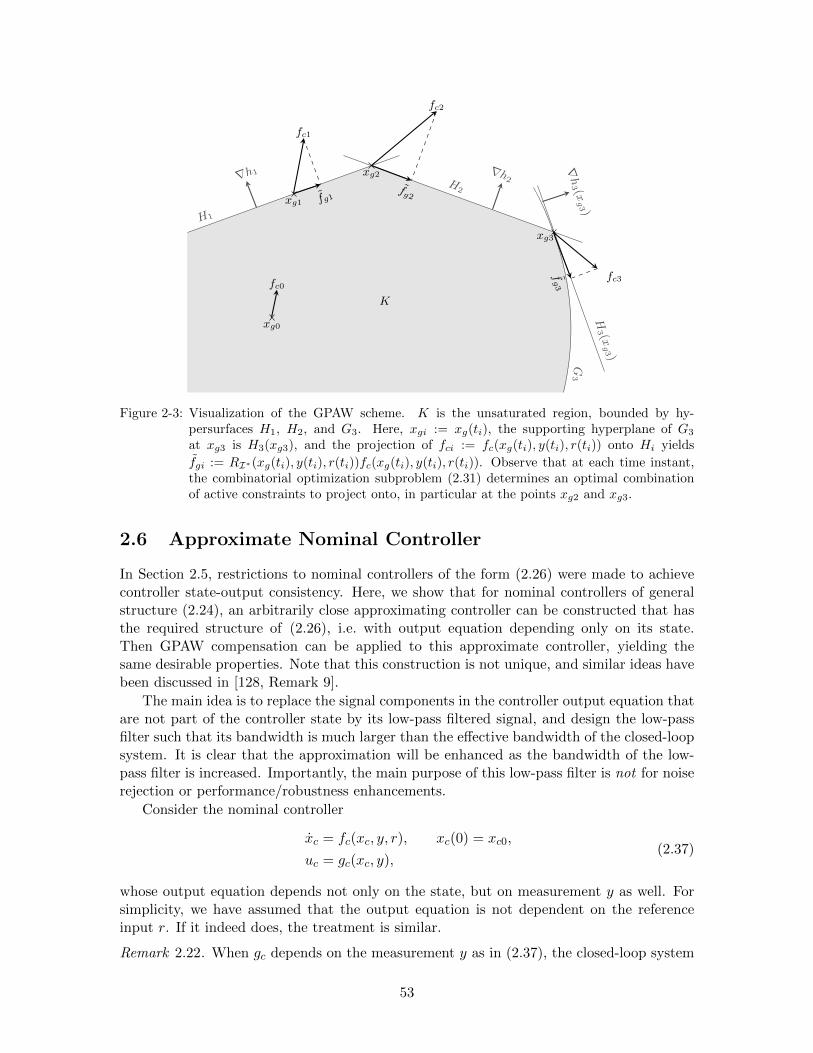
K

H1

H2

H3 (x

g3 )

∇h1 ∇h2

∇h3 (x

g3 )

G3

xg0

fc0

fg1xg1

fc1

fg2

xg2

fc2

fg3

xg3

fc3

Figure 2-3: Visualization of the GPAW scheme. K is the unsaturated region, bounded by hy-persurfaces H1, H2, and G3. Here, xgi := xg(ti), the supporting hyperplane of G3

at xg3 is H3(xg3), and the projection of fci := fc(xg(ti), y(ti), r(ti)) onto Hi yields

fgi := RI∗(xg(ti), y(ti), r(ti))fc(xg(ti), y(ti), r(ti)). Observe that at each time instant,the combinatorial optimization subproblem (2.31) determines an optimal combinationof active constraints to project onto, in particular at the points xg2 and xg3.

2.6 Approximate Nominal Controller

In Section 2.5, restrictions to nominal controllers of the form (2.26) were made to achievecontroller state-output consistency. Here, we show that for nominal controllers of generalstructure (2.24), an arbitrarily close approximating controller can be constructed that hasthe required structure of (2.26), i.e. with output equation depending only on its state.Then GPAW compensation can be applied to this approximate controller, yielding thesame desirable properties. Note that this construction is not unique, and similar ideas havebeen discussed in [128, Remark 9].

The main idea is to replace the signal components in the controller output equation thatare not part of the controller state by its low-pass filtered signal, and design the low-passfilter such that its bandwidth is much larger than the effective bandwidth of the closed-loopsystem. It is clear that the approximation will be enhanced as the bandwidth of the low-pass filter is increased. Importantly, the main purpose of this low-pass filter is not for noiserejection or performance/robustness enhancements.

Consider the nominal controller

xc = fc(xc, y, r), xc(0) = xc0,

uc = gc(xc, y),(2.37)

whose output equation depends not only on the state, but on measurement y as well. Forsimplicity, we have assumed that the output equation is not dependent on the referenceinput r. If it indeed does, the treatment is similar.

Remark 2.22. When gc depends on the measurement y as in (2.37), the closed-loop system

53

comprising the plant (2.34) and controller (2.37) with u := uc will contain an algebraic loopwhenever ∂g

∂u∂gc∂y 6≡ 0.

Consider augmenting the controller state to be xc := (xc, y), with y = y. Then, byreplacing y with y in the controller output equation, we have uc = gc(xc, y) = gc(xc), whichis the desired form in (2.26). The state equation of the augmented controller with state xcneeds to satisfy

xc = fc(xc, y, r), ˙y = y. (2.38)

Clearly, if the functions f and g in (2.34) are known exactly, realization of (2.38) is straight-forward,17 by taking the time derivative of y in (2.34) and using the knowledge of f and g.We avoid making such a conservative assumption by using an approximation.

Consider y obtained as the output of an exponentially stable, unity DC gain low-passfilter with input y, parameterized by a ∈ (0,∞)

˙y = a(y − y), y(0) = y(0).

It can be seen that y(t) → y(t) for all t ≥ 0 as a → ∞, so that the solution of theapproximating controller

xc = fc(xc, y, r), xc(0) = xc0,

˙y = a(y − y), y(0) = y(0),

uc = gc(xc, y),

(2.39)

can be made arbitrarily close to the nominal controller (2.37). While this can be shownformally for any fixed y : [0,∞) → Rp and r : [0,∞) → Rnr using singular perturbationtheory [37, Chapter 11, pp. 423 – 459], the larger question is the effect of the approximationon the closed-loop system, which we discuss next.

The closed-loop system described by the feedback interconnection of the plant (2.34)and approximate controller (2.39) with u := uc is described by

x = f(x, sat(gc(xc, y))),

xc = fc(xc, g(x, sat(gc(xc, y))), r),

ε ˙y = g(x, sat(gc(xc, y)))− y,(2.40)

where ε := 1a . Observe that when ε = 0, we recover the exact closed-loop system obtained

with controller (2.37), which corresponds to the reduced system in the singular perturbationframework. System (2.40) is referred as the approximate system when ε > 0, and the exactsystem when ε = 0. When we assume existence and uniqueness of solutions18 to the exactsystem, then (2.40) is a standard singular perturbation model [37, p. 424]. It can be shown

17When the closed-loop system contains an algebraic loop, there are additional difficulties on well-posedness of the feedback interconnection.

18Recall that in the anti-windup context, the nominal controller has been designed to achieve some desiredperformance. Existence and uniqueness of solutions to the closed-loop system is usually guaranteed evenwhen not explicitly sought in the control design.

54

that if g and gc are such that the eigenvalue condition19 [37, p. 433]

Re

(λ

(∂g

∂u

∂gc∂y

(x, xc)− I))

< 0,

holds uniformly for all (x, xc) in some domain, then the origin of the associated boundarylayer model for the singular perturbation model (2.40) is exponentially stable. With this,and assuming existence and uniqueness of solutions of the exact system, [37, Theorem 11.1,p. 434] shows that on any finite time interval, the solution of the approximate systemcan be made arbitrarily close to the solution of the exact system when ε is sufficientlysmall (or equivalently, a is sufficiently large). When the equilibrium of the exact systemis exponentially stable, [37, Theorem 11.2, pp. 439 – 440] shows that the result extends toinfinite intervals.

Observe that for input-constrained LTI systems driven by LTI controllers, local expo-nential stability is usually guaranteed, so that the infinite time approximation result holds.If the exact system is not exponentially stable and the finite time approximation result in-dicated above is not sufficient, repeating the analysis with the approximate controller maybe required. Because the approximation can be made arbitrarily well, it is likely that theapproximate controller will be able to achieve the control objectives as well.

Remark 2.23. The approximate controller (2.39) requires the augmentation of the controllerstate. We note that the (q +m)-th order controller with state (xc, uc) and output uc,

xc = fc(xc, y, r), xc(0) = xc0,

uc =∂gc(xc)

∂xcfc(xc, y, r), uc(0) = gc(xc0),

is a non-minimal (equivalent) realization of the nominal controller (2.26). For the precedingaugmented controller, it can be shown that GPAW compensation with parameter Γ = I ∈R(q+m)×(q+m) yields effectively no anti-windup compensation. This suggests that controllerstate augmentation should always be done with caution, and using a minimal realization [50]would likely be more appropriate. We leave the study of the implications of controller stateaugmentation as future work (see Section 7.1.10).

In summary, for controllers of general structure (2.24), an arbitrarily close approximat-ing controller can be constructed that has the form of (2.26), where the output equationdepends only on the controller state. Then GPAW compensation can be applied to the ap-proximate controller yielding controller state-output consistency (see Theorem 2.5.3). Theapproximate controller constructed in this section will be of higher order than the exactnominal controller. In this sense, application of the GPAW scheme on the approximatecontroller can be seen to be analogous to the case of employing dynamic anti-windup com-pensators, where additional states are employed. Sections 2.8.1, 6.1.2, and 6.2.3 illustratehow the construction presented can be applied in modified form.

Other than the basic construction presented here and Section 2.5, alternative ways torealize GPAW-compensated controllers are shown in Section 4.1 as well as Appendices Aand B. For ease of reference, we summarize the procedure to apply GPAW compensationin Appendix C.

19Here, Re(λ(A)) means real part of all eigenvalues of matrix A, and ∂g∂u

∂gc∂y

(x, xc) is shorthand for∂g∂u

(x, sat(gc(xc, h(x, xc))))∂gc∂y

(xc, h(x, xc)) where y = h(x, xc) is an isolated real root of the equationg(x, sat(gc(xc, y)))− y = 0.

55

2.7 Passivity and L2-Gain of Projection Operator

In this section, we define the principal and complementary projection operators inducedby the projection operator RI∗(xg, y, r) in (2.27), and show them to be passive and withL2-gain less than one. These results can be used in conjunction with numerous passivitybased results (e.g. [37, Chapter 6, pp. 227 – 259], [40, 41, 129]) to establish stability ofGPAW-compensated systems. First, we recall the definitions of passivity, sector bounds,and L2-gain.

Definition 2.1 (Passive Memoryless Systems [37, Definition 6.1, p. 231]). The memorylessnonlinear system y = h(t, u) is said to be

(i) passive if uTy ≥ 0 for all (t, u);(ii) lossless if uTy = 0 for all (t, u);

(iii) output strictly passive if uTy ≥ yTϕ(y) for some function ϕ and all (t, u), and yTϕ(y) >0 for all y 6= 0.

Definition 2.2 (Sector Bounds [37, Definition 6.2, pp. 232 – 233]). A memoryless functionh : [0,∞)× Rq → Rq is said to belong to the sector

(i) [0,∞] if uTh(t, u) ≥ 0 for all (t, u);(ii) [0, F ] with F = FT > 0 if hT(t, u)(h(t, u)− Fu) ≤ 0 for all (t, u).

For the definition of the L2-gain, recall that L2e(Rq) is the extended L2-space whichconsists of all measurable functions β : [0,∞)→ Rq such that [41, pp. 2 – 3]

‖βT ‖22 :=

∫ T

0‖β(t)‖2 dt <∞, ∀T ∈ [0,∞).

A map G : L2e(Rq)→ L2e(Rq) has finite L2-gain if there exist finite constants γ, b ∈ R suchthat [41, Definition 1.2.1, p. 4, Lemma 2.2.13, p. 19]

‖(G(u))T ‖22 ≤ γ2‖uT ‖22 + b, ∀u ∈ L2e(Rq),∀T ≥ 0. (2.41)

Definition 2.3 (L2-Gain [41, Lemma 2.2.13, p. 19]). The L2-gain of G : L2e(Rq)→ L2e(Rq)is defined as

γ2(G) := infγ ∈ [0,∞) | ∃b ∈ R such that (2.41) holds,with the infimum of an empty set being +∞.

Next, we define the principal and complementary projection operators induced by theprojection operator RI∗(xg, y, r) in (2.27). Since the GPAW parameter Γ ∈ Rq×q is sym-metric positive definite, it can always be decomposed as Γ = ΦΦT for some nonsingularΦ ∈ Rq×q [124, Theorem 7.2.7, p. 406]. For any I such that rank(NI(xg)) = |I|, the matrixRI(xg) (2.30) is well defined.20 For any well defined RI(xg), let the principal projectionmatrix 21 PI(xg) and complementary projection matrix SI(xg) induced by RI(xg) be

PI(xg) := Φ−1RI(xg)Φ, SI(xg) := I − PI(xg), (2.42)

so thatRI(xg) = ΦPI(xg)Φ

−1 = I − ΦSI(xg)Φ−1. (2.43)

20The embedded inverse (NTI ΓNI(xg))

−1 exists, or is not needed.21This is the same PI(xg) in the proof of Proposition 2.5.2.

56

It can be verified from (2.30) that PI(xg) and SI(xg) take the explicit forms

PI(xg) =

I − NI(NT

I NI)−1NT

I (xg), if I 6= ∅,I, otherwise,

(2.44)

SI(xg) =

NI(N

TI NI)

−1NTI (xg), if I 6= ∅,

0, otherwise,

where NI(xg) := ΦTNI(xg). From [100, Lemma 1, Theorem 1], it can be seen that bothare projection matrices. Moreover, it can be verified from the preceding definitions thatthey are idempotent [126, p. 697] and satisfy

PI(xg) = P 2I (xg) = PT

I PI(xg), SI(xg) = S2I(xg) = ST

I SI(xg). (2.45)

The principal and complementary projection operators are then given by

PI∗(xg, y, r) = Φ−1RI∗(xg, y, r)Φ, SI∗(xg, y, r) = I − PI∗(xg, y, r),

respectively, where I∗ is a solution to subproblem (2.31). It can be seen from (2.31)that rank(NI∗(xg)) = |I∗|, so that all projection operators RI∗(xg, y, r), PI∗(xg, y, r), andSI∗(xg, y, r), are well defined. The next result states that the principal and complementaryprojection operators22 are passive.

Proposition 2.7.1 (Passivity of Principal and Complementary Projection Operators). Theprojection operators

(i) w1 : Rq → Rq defined by w1 = PI∗(xg, y, r)v1; and(ii) w2 : Rq → Rq defined by w2 = SI∗(xg, y, r)v2,

are output strictly passive, satisfying vTi wi = wT

i wi ≥ 0 for i ∈ 1, 2.

Proof. Consider case (i). From (2.45), we have

vT1 w1 = vT

1 PI∗(xg, y, r)v1 = vT1 P

TI∗(xg, y, r)PI∗(xg, y, r)v1 = wT

1 w1 ≥ 0.

Defining ϕ(w1) := w1 for all w1, we have wT1 ϕ(w1) = wT

1 w1 > 0 for all w1 6= 0, which provesthe conclusion for case (i). Case (ii) is proved similarly by invoking the idempotence ofSI∗(xg, y, r) (2.45).

From Proposition 2.7.1, we have wTi (wi − Ivi) = 0 ≤ 0 for i ∈ 1, 2, so that both

w1 and w2 belong to the sector [0, I] with I the identity matrix (see Definition 2.2). Thisimplies that they also belong to the sector [0,∞]. Being in the sector [0, I] allows the useof output-feedback (see Fig. 2-4) to yield passive maps that belong to the sector [0,∞] [37,pp. 255 – 259]. By defining vi := vi − wi and wi := wi, it can be seen that vT

i wi = 0 ≥ 0,which show the systems in Fig. 2-4 to be lossless (and passive). The L2-gain bound of theprojection maps are presented next.

Proposition 2.7.2 (L2-Gain Bound of Projection Maps). For any well defined trajectory(xg(t), y(t), r(t)) ∈ Rq+p+nr for all t ∈ [0,∞), let I∗(t) be a solution to subproblem (2.31)at time t. The L2-gain of the projection maps

22Both the map and its associated matrix are called operators.

57

PI∗(xg, y, r) SI∗(xg, y, r)v1 w1 v2 w2

Figure 2-4: Unity positive output feedback yields lossless (passive) operators belonging to the sector[0,∞], with vTi wi = 0 for i ∈ 1, 2.

(i) w1 : L2e(Rq) → L2e(Rq) defined by w1(t) = PI∗(t)(xg(t), y(t), r(t))v1(t) for all t ∈[0,∞); and

(ii) w2 : L2e(Rq) → L2e(Rq) defined by w2(t) = SI∗(t)(xg(t), y(t), r(t))v2(t) for all t ∈[0,∞),

satisfy the bound γ2(wi) ≤ 1 for i ∈ 1, 2, where γ2 is defined in Definition 2.3.

Proof. The proof is similar to that of [37, Lemma 6.5, p. 242]. By Proposition 2.7.1, fori ∈ 1, 2 and each t ∈ [0,∞), we have vT

i (t)wi(t) = wTi (t)wi(t), so that

0 = wTi (t)wi(t)− vT

i (t)wi(t),

= 12(wi(t)− vi(t))T(wi(t)− vi(t)) + 1

2

(wTi (t)wi(t)− vT

i (t)vi(t)),

≥ 12

(wTi (t)wi(t)− vT

i (t)vi(t)).

Rearranging terms and taking the integral over [0, T ] yields∫ T

0‖wi(t)‖2 dt ≤

∫ T

0‖vi(t)‖2 dt, ∀T ≥ 0,

so that ‖(wi)T ‖22 ≤ ‖(vi)T ‖22 for all T ≥ 0. Hence (2.41) holds with b = 0 and γ = 1, whichimplies the conclusion (see Definition 2.3).

Remark 2.24. Proposition 2.7.2 can be used to derive small-gain type [37, Theorem 5.6,p. 218] stability conditions for the GPAW-compensated system.

Remark 2.25. Since Γ = ΦΦT, it can be shown that the L2-gain of the projection operatorRI∗(xg, y, r) = ΦPI∗(xg, y, r)Φ

−1 is bounded above by ‖Φ‖‖Φ−1‖ = κ(Φ), where κ(A) isthe condition number of matrix A [124, p. 336]. This can be related to the condition numberof Γ = ΓT > 0 through

κ(Φ) = ‖Φ‖‖Φ−1‖ =√λmax(ΦTΦ)

√λmax(Φ−TΦ−1) =

√λmax(ΦTΦ)√λmin(ΦΦT)

=

√λmax(ΦΦT)√λmin(ΦΦT)

,

=

√λmax(Γ)

λmin(Γ)=

√λ2max(Γ)√λ2

min(Γ)

12

=

(√λmax(Γ2)√λmin(Γ2)

) 12

=

(√λmax(ΓTΓ)√λmin(ΓΓT)

) 12

=√κ(Γ),

where we have used λmax(A) = 1λmin(A−1)

for A = AT > 0, λ(ATA) = λ(AAT), and

λ2(A) = λ(A2). While this bound may not be tight, it suggests that the GPAW parametershould be chosen so that it is not ill-conditioned, i.e. choose Γ so that κ(Γ) 6 1.

The GPAW-compensated system (2.35) is illustrated in Fig. 2-5 with the projection op-erator RI∗(xg, y, r) = ΦPI∗(xg, y, r)Φ

−1. Observe that the nominal uncompensated systemis obtained by replacing RI∗(xg, y, r) with the identity matrix. We leave the developmentof results based on Propositions 2.7.1 and 2.7.2 as future work (see Section 7.1.7).

58

fc(xg, y, r) Φ−1 PI∗ Φxg = w

u = gc(xg)

sat(u)x = f(x, u)

y = g(x, u)

v w

u

r

u

y

xg

RI∗

Figure 2-5: Closed-loop GPAW-compensated system as the uncompensated system modified by apassive operator PI∗ (with L2-gain less than 1) and two constant transformation matri-ces, Φ,Φ−1.

2.8 GPAW Compensation on a Two-link Robot Driven byan Adaptive Sliding Mode Controller

x1

x2

Figure 2-6: Nonlinear two-link robot.

To illustrate the pertinent features of GPAW compensation, we apply the GPAW scheme ona two-link robot (illustrated in Fig. 2-6) driven by an adaptive sliding mode controller [38,pp. 404 – 408], [102]. The model23 of a saturated nonlinear two-link robot is given by [38,p. 393]

H(xt)xt + C(xt, xt)xt = sat(u), (2.46)

where sat(·) is the saturation function in (1.2), the truncated or partial state xt = [x1, x2]T,and xt, xt, are the vectors of joint angles, velocities, and accelerations respectively, andu = [u1, u2]T is the vector of input joint torques. In (2.46), H(xt) ∈ R2×2 is the symmetricinertia matrix, and C(xt, xt)xt ∈ R2 is the vector of centripetal and Coriolis torques, definedby [38, p. 396]

H(xt) =

[H11(x2) H12(x2)H12(x2) H22

], C(xt, xt) = h(x2)

[−x2 −x1 − x2

x1 0

], (2.47)

H11(x2) = hT11a, H12(x2) = hT

12a, H22 = hT22a, h(x2) = hT

0 a,

h11 := h11(x2) = [1, 0, 2 cosx2, 2 sinx2]T, h12 := h12(x2) = [0, 1, cosx2, sinx2]T,

h22 := h22(x2) = [0, 1, 0, 0]T, h0 := h0(x2) = [0, 0, sinx2,− cosx2]T,

23The movement of the two-link robot is confined to the horizontal plane so that gravitational torques arenot involved. Moreover, we have used (xt, x1, x2, sat(u)) in place of (q, q1, q2, τ) in [38, p. 393].

59

and a := [a1, a2, a3, a4]T = [3.34, 0.97, 3√

3/5, 0.6]T is a vector of constant system param-eters. As observed in [38, p. 394], the inertia matrix H(xt) is uniformly positive definite,i.e. there exists a constant α > 0 such that H(xt) ≥ αI for all xt ∈ R2, so that the inverseH−1(xt) exists for all xt ∈ R2. Then system (2.46) can be written in the form of (2.34),with state x := [x1, x2, x3, x4]T := [x1, x2, x1, x2]T = (xt, xt) and

f(x, sat(u)) =

x3,x4,

H−1(xt)(−C(xt, xt)xt + sat(u))

, g(x, sat(u)) = x.

Observe that the definition of the output function g implies the entire state x is availableto the controller.

An adaptive sliding mode controller for the two-link robot is described by [38, Sec-tion 9.2.1, pp. 404 – 408]

˙a = −ΘY Ts, a(0) = a0,

uc = Y a−KDs,(2.48)

where24

s = et + Λet = xt − xtr, et = xt − xtd, xtr = xtd − Λet = [xtr1, xtr2]T, (2.49)

and the matrix Y := Y (x, xtr, xtr) is defined by

H(xt)xtr + C(xt, xt)xtr = Y (x, xtr, xtr)a. (2.50)

Here, Θ = ΘT > 0 ∈ R4×4, KD = KTD > 0 ∈ R2×2, and Λ = ΛT > 0 ∈ R2×2 are

chosen constant controller parameters (or gains), and xtd(t) ∈ R2, t ∈ [0,∞), is the desiredreference trajectory for the joint angles xt. We fix the controller parameters as

Θ = diag(30, 1, 10, 10), KD = 10I, Λ = I, (2.51)

for all (derivative) controllers to be defined, where diag(x1, . . . , xi) is the diagonal matrixwith (x1, . . . , xi) as its ordered diagonal entries. The reference trajectory is fixed to be thesinusoid25

xtd(t) = π(1− cos(2πt))[

16 ,

14

]T, (2.52)

which may represent a pick-and-place operation. Using (2.47) to expand the left-hand-sideof (2.50) yields[

hT11a hT

12ahT

12a hT22a

] [xtr1xtr2

]+ hT

0 a

[−x2 −x1 − x2

x1 0

] [xtr1xtr2

]=

[xtr1h

T11 + xtr2h

T12

xtr1hT12 + xtr2h

T22

]a+

[−x2 −x1 − x2

x1 0

] [xtr1xtr2

]hT

0 a,

=

[xtr1h

T11 + xtr2h

T12 − (xtr1x2 + xtr2(x1 + x2))hT

0

xtr1hT12 + xtr2h

T22 + xtr1x1h

T0

]a = Y a,

24We have used (Θ, uc, et, xtr, xtd) in place of (Γ, τ, q, qr, qd) in the description of the adaptive sliding modecontroller in [38, Section 9.2.1, pp. 404 – 408].

25This choice of reference trajectory implies xtd(t) = 2π2 sin(2πt)[ 16, 14]T and xtd(t) = 4π3 cos(2πt)[ 1

6, 14]T.

60

which gives the expressions for elements of the matrix Y = [yij ] ∈ R2×4 as

y11 = xtr1, y12 = xtr2, y23 = xtr1 cosx2 + xtr1x1 sinx2,

y21 = 0, y22 = xtr1 + xtr2, y24 = xtr1 sinx2 − xtr1x1 cosx2,

y13 = (2xtr1 + xtr2) cosx2 − (xtr1x2 + xtr2(x1 + x2)) sinx2,

y14 = (2xtr1 + xtr2) sinx2 + (xtr1x2 + xtr2(x1 + x2)) cosx2.

(2.53)

The adaptive sliding mode controller (2.48) was designed particularly for the case when thesystem parameters a = [a1, a2, a3, a4]T are unknown. Observe that the reference trajectoryand its time derivatives (xtd, xtd, xtd) are required to realize (2.48). The closed-loop systemcomprising the plant (2.46) and controller (2.48) with u = uc will be called the nominalsystem and denoted by Σn. If the plant is unconstrained, i.e. umax,i = −umin,i = ∞ fori ∈ 1, 2, the same closed-loop system (2.46), (2.48), will be called the unconstrainedsystem and denoted by Σu. As shown in [38, pp. 405 – 406], the unconstrained system Σu

achieves global stability and convergence of tracking error, i.e. boundedness of (x(t), a(t))for all t ∈ [0,∞) and (et(t), et(t))→ (0, 0) as t→∞.

Now, observe from (2.49) that s is a function of (xt, xt, xtd, xtd) = (x, xtd, xtd), and xtris a function of (xt, xtd, xtd). In turn, these show xtr to be a function of (xt, xtd, xtd) andY = Y (x, xtr, xtr) to be a function of (x, xtd, xtd, xtd). By defining26

xc := a, y := x, r := (xtd, xtd, xtd),

it is clear that the adaptive sliding mode controller (2.48) is of the form (2.24), with outputequation being

gc(xc, y, r) = Y a−KDs = Y (y, r)xc −KDs(y, r). (2.54)

However, to achieve controller state-output consistency (see Theorem 2.5.3), the nominalcontroller needs to be of the form (2.26), which we discuss next.

2.8.1 Approximate Nominal Controller

We will use techniques similar to those in Section 2.6 to derive an approximate nominalcontroller of the form (2.26) from the adaptive sliding mode controller (2.48). First, observefrom the output equation (2.54) that we need to approximate Y and s. If approximationsof both measurement and reference input (y, r) = (x, xtd, xtd, xtd) ∈ R10 are used as inSection 2.6, we need to augment the controller state by 10 additional state variables. Alsorecall Remark 2.23 which cautions against excessive controller state augmentation. Exam-ine (2.53) to see that the matrix Y can be approximated if we have estimates of the 5 signals(xtr1, xtr2, x2, xtr1x1, xtr1x2 + xtr2(x1 + x2)). Adding 2 more signals, namely the elementsof s, requires a total of 7 (< 10) augmented state variables.

Hence define the approximation xcaug := [xc5, xc6, . . . , xc11]T of these 7 signals by aparameter b > 0 as

xcaug = b(zin − xcaug), xcaug(0) = zin(0) := zin(y(0), r(0)),

zin := [xtr1, xtr2, x2, xtr1x1, xtr1x2 + xtr2(x1 + x2), sT(y, r)]T.(2.55)

The matrix Y can then be approximated as Y = [yij ], whose elements are defined by

26Note that y is the measurement, and does not correspond to elements of Y = [yij ].

61

0 1 2 3 4 5 6 7 8 9 10−0.5

0

0.5

1

e t1(deg)

0 1 2 3 4 5 6 7 8 9 10−4

−2

0

2

4

e t2(deg)

time (s)

0 1 2 3 4 5 6 7 8 9 10−400

−200

0

200

400

u1(N

m)

0 1 2 3 4 5 6 7 8 9 10−200

−100

0

100

200

u2(N

m)

time (s)

Σu

Σua50

Σua100

Σua1000

Figure 2-7: Time responses of unconstrained approximate system Σua for b ∈ 50, 100, 1000 com-pared to the response of the unconstrained system Σu. Observe that the responses ofsystems Σu and Σua1000 are almost indistinguishable.

(compare with (2.53))

y11 = xc5, y12 = xc6, y23 = xc5 cosxc7 + xc8 sinxc7,

y21 = 0, y22 = xc5 + xc6, y24 = xc5 sinxc7 − xc8 cosxc7,

y13 = (2xc5 + xc6) cosxc7 − xc9 sinxc7,

y14 = (2xc5 + xc6) sinxc7 + xc9 cosxc7.

(2.56)

Since s := [xc10, xc11]T is an approximation of s(y, r), we can define the augmented statexc := (xc, xcaug) ∈ R11 to write the augmented nominal controller as

xc = −ΘY T(y, r)s(y, r), xc(0) = a0,

xcaug = b(zin(y, r)− xcaug), xcaug(0) = zin(0),

uc = Y (xcaug)xc −KDs(xcaug) = gc(xc).

(2.57)

It is clear that the approximation will be improved as b → ∞. The closed-loop systemcomprising the plant (2.46) and approximate controller (2.57) with u = uc will be called thenominal approximate system and denoted by Σna. If the plant is unconstrained, i.e. umax,i =−umin,i = ∞ for i ∈ 1, 2, the same closed-loop system (2.46), (2.57) will be called theunconstrained approximate system and denoted by Σua.

To choose the approximation parameter b, we simulate and compare the time responsesof the unconstrained system Σu and unconstrained approximate system Σua for differentvalues of b. It was found numerically that setting b = 27 yields an unstable Σua, while withb = 28, system Σua is stable but with poor performance. Systems Σu and Σua were comparedfor values of b ∈ (50, 60, . . . , 90, 100 ∪ 150, 200, . . . , 950, 1000). Time responses of threecases corresponding to b ∈ 50, 100, 1000 are shown in Fig. 2-7, with system Σua denotedby (Σua50,Σua100,Σua1000) respectively. In Fig. 2-7, the tracking errors et = [et1, et2]T

(see (2.49)) are shown together with the joint torques u = [u1, u2]T. Observe that the timeresponses of Σu and Σua1000 (for b = 1000) are almost indistinguishable in Fig. 2-7.

62

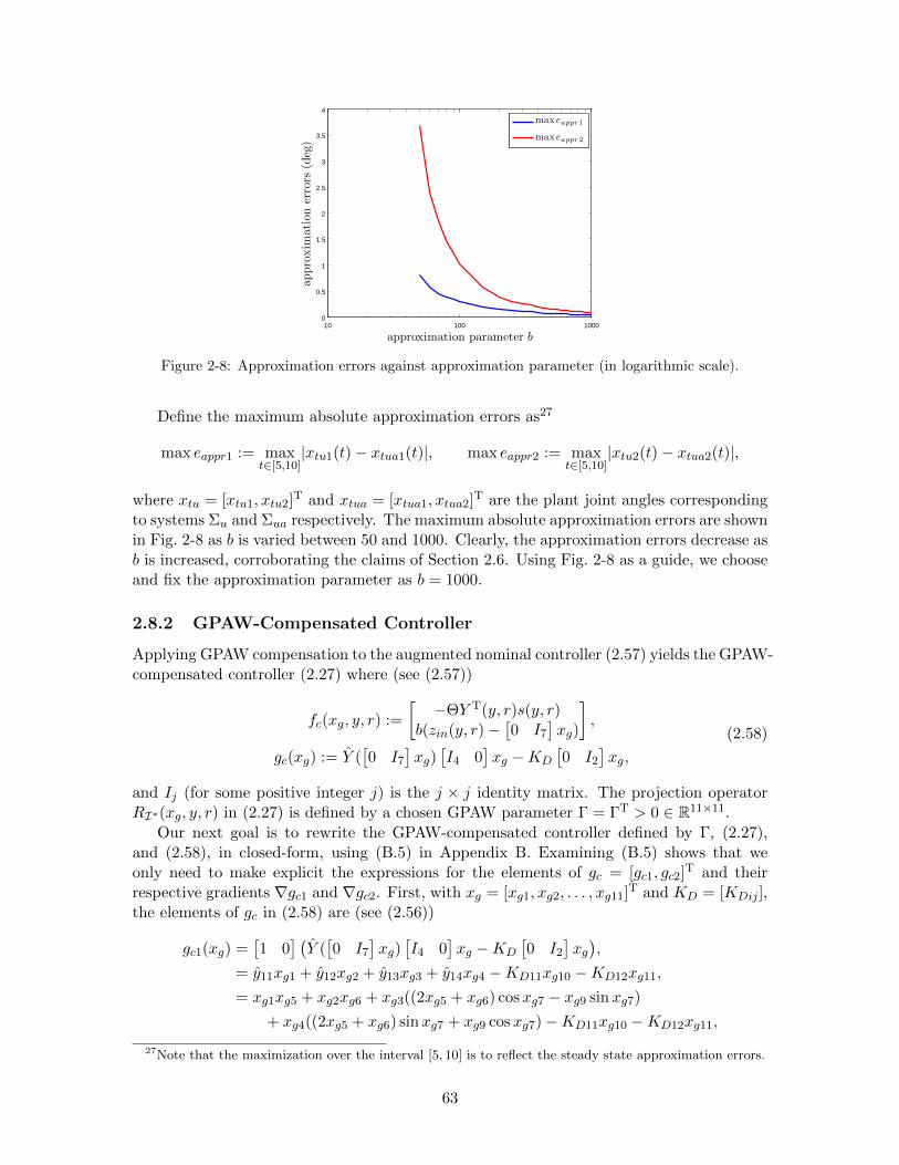
10 100 10000

0.5

1

1.5

2

2.5

3

3.5

4

approxim

ationerrors

(deg)

approximation parameter b

maxeappr1

maxeappr2

Figure 2-8: Approximation errors against approximation parameter (in logarithmic scale).

Define the maximum absolute approximation errors as27

max eappr1 := maxt∈[5,10]

|xtu1(t)− xtua1(t)|, max eappr2 := maxt∈[5,10]

|xtu2(t)− xtua2(t)|,

where xtu = [xtu1, xtu2]T and xtua = [xtua1, xtua2]T are the plant joint angles correspondingto systems Σu and Σua respectively. The maximum absolute approximation errors are shownin Fig. 2-8 as b is varied between 50 and 1000. Clearly, the approximation errors decrease asb is increased, corroborating the claims of Section 2.6. Using Fig. 2-8 as a guide, we chooseand fix the approximation parameter as b = 1000.

2.8.2 GPAW-Compensated Controller

Applying GPAW compensation to the augmented nominal controller (2.57) yields the GPAW-compensated controller (2.27) where (see (2.57))

fc(xg, y, r) :=

[−ΘY T(y, r)s(y, r)

b(zin(y, r)−[0 I7

]xg)

],

gc(xg) := Y ([0 I7

]xg)[I4 0

]xg −KD

[0 I2

]xg,

(2.58)

and Ij (for some positive integer j) is the j × j identity matrix. The projection operatorRI∗(xg, y, r) in (2.27) is defined by a chosen GPAW parameter Γ = ΓT > 0 ∈ R11×11.

Our next goal is to rewrite the GPAW-compensated controller defined by Γ, (2.27),and (2.58), in closed-form, using (B.5) in Appendix B. Examining (B.5) shows that weonly need to make explicit the expressions for the elements of gc = [gc1, gc2]T and theirrespective gradients ∇gc1 and ∇gc2. First, with xg = [xg1, xg2, . . . , xg11]T and KD = [KDij ],the elements of gc in (2.58) are (see (2.56))

gc1(xg) =[1 0

] (Y ([0 I7

]xg)[I4 0

]xg −KD

[0 I2

]xg),

= y11xg1 + y12xg2 + y13xg3 + y14xg4 −KD11xg10 −KD12xg11,

= xg1xg5 + xg2xg6 + xg3((2xg5 + xg6) cosxg7 − xg9 sinxg7)

+ xg4((2xg5 + xg6) sinxg7 + xg9 cosxg7)−KD11xg10 −KD12xg11,

27Note that the maximization over the interval [5, 10] is to reflect the steady state approximation errors.

63

gc2(xg) =[0 1

] (Y ([0 I7

]xg)[I4 0

]xg −KD

[0 I2

]xg),

= y21xg1 + y22xg2 + y23xg3 + y24xg4 −KD21xg10 −KD22xg11,

= xg2(xg5 + xg6) + xg3(xg5 cosxg7 + xg8 sinxg7)

+ xg4(xg5 sinxg7 − xg8 cosxg7)−KD21xg10 −KD22xg11.

Their respective gradients ∇gc1 = [∇gc1,1, . . . ,∇gc1,11]T, ∇gc2 = [∇gc2,1, . . . ,∇gc2,11]T, canthen be evaluated, whose elements are

∇gc1,1 = xg5, ∇gc2,1 = 0,

∇gc1,2 = xg6, ∇gc2,2 = xg5 + xg6,

∇gc1,3 = (2xg5 + xg6) cosxg7 − xg9 sinxg7, ∇gc2,3 = xg5 cosxg7 + xg8 sinxg7,

∇gc1,4 = (2xg5 + xg6) sinxg7 + xg9 cosxg7, ∇gc2,4 = xg5 sinxg7 − xg8 cosxg7,

∇gc1,5 = xg1 + 2xg3 cosxg7 + 2xg4 sinxg7, ∇gc2,5 = xg2 + xg3 cosxg7 + xg4 sinxg7,

∇gc1,6 = xg2 + xg3 cosxg7 + xg4 sinxg7, ∇gc2,6 = xg2,

∇gc1,7 = (−xg3xg9 + xg4(2xg5 + xg6)) cosxg7 ∇gc2,7 = (xg3xg8 + xg4xg5) cosxg7

− (xg3(2xg5 + xg6) + xg4xg9) sinxg7, + (−xg3xg5 + xg4xg8) sinxg7,

∇gc1,8 = 0, ∇gc2,8 = xg3 sinxg7 − xg4 cosxg7,

∇gc1,9 = −xg3 sinxg7 + xg4 cosxg7, ∇gc2,9 = 0,

∇gc1,10 = −KD11, ∇gc2,10 = −KD21,

∇gc1,11 = −KD12, ∇gc2,11 = −KD22.

With the preceding expressions for gc1, gc2, ∇gc1, and ∇gc2, the closed-form expressions forthe GPAW-compensated controller (2.27), (2.58), is given by (B.5). The closed-loop systemcomprising the plant (2.46) and GPAW-compensated controller (2.27), (2.58), with u = ugwill be called the GPAW-compensated system and denoted by Σg.

2.8.3 Constrained Control

Recall that the inertia matrix H(xt) in (2.46) is uniformly positive definite, i.e. H(xt) ≥ αIfor some α > 0, and is defined by the system parameters a and joint angle x2 (see (2.47)).Moreover, the controller state a in (2.48) has the interpretation as an estimate of theunknown system parameters a [38, p. 404]. This induces an estimate of the inertia matrix,defined by a instead of a (see (2.47)). For the augmented approximate controller (2.57) andGPAW-compensated controller (2.27) defined by (2.58), the partial states xc in (2.57) and[I4, 0]xg in (2.58) will have the same interpretation as estimates of the system parametera. Here, we use ideas described in Remark 2.20 to enforce the positive semidefinitenessof the inertia matrix estimate, with the goal of enhancing system performance. Positivesemidefiniteness of the inertia matrix estimate is a reasonable goal when α > 0 in therelation H(xt) ≥ αI is unknown.

First, we derive necessary and sufficient conditions for a 2×2 symmetric matrix A = [Aij ]to be positive semidefinite.28 Recall that A = AT is positive semidefinite if and only if allits eigenvalues are non-negative [124, Theorem 7.2.1, p. 402]. Its eigenvalues λ1, λ2 are roots

28The conditions presented yields two inequalities. Other necessary and sufficient conditions are possible,with perhaps more than two inequalities.

64

of the characteristic polynomial det(λI −A) = 0, which can be verified to be

λ1(A) = 12

(A11 +A22 +

√(A11 +A22)2 − 4(A11A22 −A2

12)),

λ2(A) = 12

(A11 +A22 −

√(A11 +A22)2 − 4(A11A22 −A2

12)). (2.59)

Clearly, we have λ1 ≥ λ2, and A will be positive semidefinite if and only if λ2 ≥ 0. Byinspection of the expression for λ2, we see that λ2 ≥ 0 (and A = AT is positive semidefinite)if and only if

A11 +A22 ≥ 0, A11A22 −A212 ≥ 0. (2.60)

Next, we add constraints to the basic formulation of the GPAW-compensated con-troller to enforce the positive semidefiniteness of the inertia matrix estimate. Observefrom (2.55) that x2 is the third component of zin ∈ R7. Decomposing the state asxg = [xg1, xg2, . . . , xg11]T, it can be seen from the definition of fc in (2.58) that xg7 (thethird component of [0, I7]xg) is an estimate of the third component of zin, so that it is anestimate of the joint angle x2. Then we can define the inertia matrix estimate H(xg) as(compare with (2.47))

H(xg) =

[H11(xg) H12(xg)

H12(xg) H22(xg)

],

H11(xg) = xg1 + 2(xg3 cosxg7 + xg4 sinxg7),

H12(xg) = xg2 + xg3 cosxg7 + xg4 sinxg7,

H22(xg) = xg2.

(2.61)

From (2.60), necessary and sufficient conditions for the inertia matrix estimate H(xg) to bepositive semidefinite are

H11(xg) + H22(xg) ≥ 0, H11(xg)H22(xg)− H212(xg) ≥ 0.

To enforce positive semidefiniteness of H(xg), define the two constraints

h5(xg) = −H11(xg)− H22(xg),

= −xg1 − xg2 − 2(xg3 cosxg7 + xg4 sinxg7) ≤ 0,

h6(xg) = −H11(xg)H22(xg) + H212(xg),

= xg2(xg2 − xg1) + (xg3 cosxg7 + xg4 sinxg7)2 ≤ 0,

(2.62)

in addition to the four saturation constraints hi(xg) ≤ 0, i ∈ I4, defined by (2.28). Therespective gradients ∇h5(xg) = [∇h5,1, . . . ,∇h5,11]T and ∇h6(xg) = [∇h6,1, . . . ,∇h6,11]T

can be evaluated, whose non-zero elements can be verified to be

∇h5,1 = −1, ∇h6,1 = −xg2,∇h5,2 = −1, ∇h6,2 = −xg1 + 2xg2,

∇h5,3 = −2 cosxg7, ∇h6,3 = 2 cosxg7(xg3 cosxg7 + xg4 sinxg7),

∇h5,4 = −2 sinxg7, ∇h6,4 = 2 sinxg7(xg3 cosxg7 + xg4 sinxg7),

∇h5,7 = 2(xg3 sinxg7 − xg4 cosxg7), ∇h6,7 = 2(xg3 cosxg7 + xg4 sinxg7)

× (−xg3 sinxg7 + xg4 cosxg7).

With the addition of the two constraints (2.62), construction of the constrained controller

65

proceeds similarly as the construction of the GPAW-compensated controller in Section 2.5,resulting in a controller of similar description as (2.27). Theorem 2.5.3 can be modified toshow that if there exists a T ∈ R such that H(xg(T )) ≥ 0, then H(xg(t)) ≥ 0 holds for allt ≥ T .

As will be shown in Section 4.1, the GPAW-compensated controller (2.27) (and hencethe constrained controller with additional constraints (2.62)) can be realized as (4.11)

xg = Φx∗(xg, y, r), xg(0) = xc0,

ug = gc(xg),(2.63)

where Φ ∈ R11×11 is defined by a decomposition of the parameter Γ = ΦΦT [124, Theo-rem 7.2.7, p. 406], and x∗ is the unique solution to the convex quadratic program (4.12)

minx∈R11

‖Φ−1fc(xg, y, r)− x‖2,

subject to NTIsat(xg)Φx ≤ 0.

(2.64)

In the implementation, we use the matrix square root for Φ, i.e. Φ =√

Γ. See Section 4.1.1for guidelines to initialize the quadratic program solver. In the preceding, the functionsfc and gc are defined in (2.58), and the definition of the active constraint set Isat needsto be modified to Isat := Isat(xg) = i ∈ I6 | hi(xg) ≥ 0 to include the additionalconstraints (2.62). To solve (2.64), note that the matrix NIsat(xg) can be constructed from∇hi(xg) for i ∈ I6. The gradients ∇hi(xg) for i ∈ I4 are (see (2.28))

∇h1(xg) = ∇gc1(xg), ∇h2(xg) = ∇gc2(xg),

∇h3(xg) = −∇gc1(xg), ∇h4(xg) = −∇gc2(xg),

and ∇gc1(xg),∇gc2(xg) can be evaluated as shown in Section 2.8.2. The closed-loop systemcomprising the plant (2.46) and constrained controller (2.63), (2.58), with u = ug will becalled the constraint controlled system and denoted by ΣH .

2.8.4 Numerical Results

First, observe that the four systems Σu, Σua, Σn, and Σna have been fully defined bythe controller parameters in (2.51) and approximation parameter b (= 1000). For theGPAW-compensated system Σg (see Section 2.8.2), it was found empirically that the GPAWparameter Γ := diag(Θ, 10−4I7), where Θ is defined in (2.51), yields a stabilizing GPAW-compensated controller (2.27), (2.58). For the constraint controlled system ΣH (see Sec-tion 2.8.3), the same GPAW parameter induces a stabilizing constrained controller (2.63)with parameter Φ :=

√Γ, that enforces positive semidefiniteness of the inertia matrix es-

timate H(xg) (2.61). Using the reference trajectory (2.52), the four systems Σn, Σna, Σg,ΣH , are simulated for seven saturation levels,

umax,i = −umin,i = ulim ∈ ∞, 180, 150, 120, 90, 60, 30 Nm, ∀i ∈ 1, 2.

Notice that when ulim = ∞ Nm, systems Σn and Σna correspond to systems Σu and Σua

respectively. The initial conditions used for all four systems are

(xt(0), xt(0)) = (0, 0), a0 = 0, xcaug(0) = zin(0), xc0 = (a0, xcaug(0)),

66

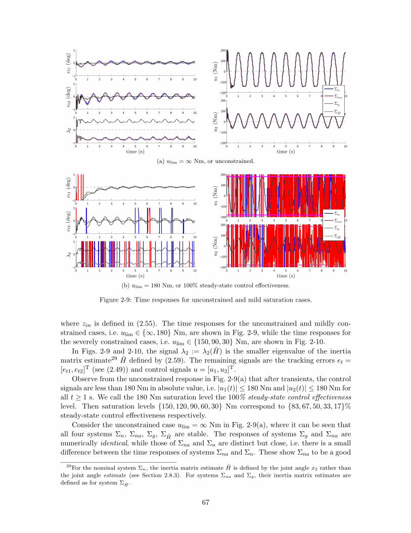
0 1 2 3 4 5 6 7 8 9 10−1

0

1

e t1(deg)

0 1 2 3 4 5 6 7 8 9 10−1

0

1

e t2(deg)

0 1 2 3 4 5 6 7 8 9 10−1

0

1

λ2

time (s)

0 1 2 3 4 5 6 7 8 9 10−200

−100

0

100

200

u1(N

m)

0 1 2 3 4 5 6 7 8 9 10−200

−100

0

100

200

u2(N

m)

time (s)

Σn

Σna

Σg

ΣH

(a) ulim =∞ Nm, or unconstrained.

0 1 2 3 4 5 6 7 8 9 10−1

0

1

e t1(deg)

0 1 2 3 4 5 6 7 8 9 10−1

0

1

e t2(deg)

0 1 2 3 4 5 6 7 8 9 10−1

0

1

λ2

time (s)

0 1 2 3 4 5 6 7 8 9 10−200

−100

0

100

200

u1(N

m)

0 1 2 3 4 5 6 7 8 9 10−200

−100

0

100

200

u2(N

m)

time (s)

Σn

Σna

Σg

ΣH

(b) ulim = 180 Nm, or 100% steady-state control effectiveness.

Figure 2-9: Time responses for unconstrained and mild saturation cases.

where zin is defined in (2.55). The time responses for the unconstrained and mildly con-strained cases, i.e. ulim ∈ ∞, 180 Nm, are shown in Fig. 2-9, while the time responses forthe severely constrained cases, i.e. ulim ∈ 150, 90, 30 Nm, are shown in Fig. 2-10.

In Figs. 2-9 and 2-10, the signal λ2 := λ2(H) is the smaller eigenvalue of the inertiamatrix estimate29 H defined by (2.59). The remaining signals are the tracking errors et =[et1, et2]T (see (2.49)) and control signals u = [u1, u2]T.

Observe from the unconstrained response in Fig. 2-9(a) that after transients, the controlsignals are less than 180 Nm in absolute value, i.e. |u1(t)| ≤ 180 Nm and |u2(t)| ≤ 180 Nm forall t ≥ 1 s. We call the 180 Nm saturation level the 100% steady-state control effectivenesslevel. Then saturation levels 150, 120, 90, 60, 30 Nm correspond to 83, 67, 50, 33, 17%steady-state control effectiveness respectively.

Consider the unconstrained case ulim =∞ Nm in Fig. 2-9(a), where it can be seen thatall four systems Σn, Σna, Σg, ΣH are stable. The responses of systems Σg and Σna arenumerically identical, while those of Σna and Σn are distinct but close, i.e. there is a smalldifference between the time responses of systems Σna and Σn. These show Σna to be a good

29For the nominal system Σn, the inertia matrix estimate H is defined by the joint angle x2 rather thanthe joint angle estimate (see Section 2.8.3). For systems Σna and Σg, their inertia matrix estimates aredefined as for system ΣH .

67

0 1 2 3 4 5 6 7 8 9 10−10

−5

0

e t1(deg)

0 1 2 3 4 5 6 7 8 9 10−4

−2

0

2

e t2(deg)

0 1 2 3 4 5 6 7 8 9 10−4

−2

0

2

λ2

time (s)

0 1 2 3 4 5 6 7 8 9 10−200

−100

0

100

200

u1(N

m)

0 1 2 3 4 5 6 7 8 9 10−200

−100

0

100

200

u2(N

m)

time (s)

Σg

ΣH

(a) ulim = 150 Nm, or 83% steady-state control effectiveness.

0 1 2 3 4 5 6 7 8 9 10−50

0

50

100

e t1(deg)

0 1 2 3 4 5 6 7 8 9 10−20

0

20

e t2(deg)

0 1 2 3 4 5 6 7 8 9 10−20

−10

0

λ2

time (s)

0 1 2 3 4 5 6 7 8 9 10−100

−50

0

50

100

u1(N

m)

0 1 2 3 4 5 6 7 8 9 10−100

−50

0

50

100

u2(N

m)

time (s)

Σg

ΣH

(b) ulim = 90 Nm, or 50% steady-state control effectiveness.

0 1 2 3 4 5 6 7 8 9 10−100

0

100

e t1(deg)

0 1 2 3 4 5 6 7 8 9 10−20

0

20

40

e t2(deg)

0 1 2 3 4 5 6 7 8 9 10−20

−10

0

λ2

time (s)

0 1 2 3 4 5 6 7 8 9 10−50

0

50

u1(N

m)

0 1 2 3 4 5 6 7 8 9 10−40

−20

0

20

40

u2(N

m)

time (s)

Σg

ΣH

(c) ulim = 30 Nm, or 17% steady-state control effectiveness.

Figure 2-10: Time responses for severe saturation cases. The responses of systems Σn and Σna areunstable (see Fig. 2-9(b) for an example), and excluded to prevent clutter.

68

approximation of Σn, and Σg recovers the response of the nominal approximate system Σna

when the saturation limits are not triggered. Observe that system ΣH exhibits superiortracking performance when compared to systems Σn, Σna, and Σg. Moreover, signal λ2 forsystem ΣH is always non-negative, which shows the inertia matrix estimate H to be always

positive semidefinite. In contrast, the inertia matrix estimate H for systems Σn, Σna, andΣg are not always positive semidefinite. Since for system ΣH , the nominal system response(those of either Σn or Σna) is not recovered when saturation constraints are not triggered, itis not an anti-windup compensated system. This is expected because the constraints to en-force positive semidefiniteness of H may be triggered irrespective of any control saturation.Non-negativity of λ2 (and hence positive semidefiniteness of H) is also seen in Figs. 2-9(b)and 2-10. These show the effectiveness of the constrained controller (2.63) in enforcing theadditional constraints (2.62).

In Fig. 2-9(b), we see that systems Σn and Σna became unstable. This is also the casefor the remaining saturated cases in Fig. 2-10. To prevent clutter, the responses of systemsΣn and Σna are omitted in Fig. 2-10.

For the saturated cases ulim ∈ 180, 150, 90, 30 Nm in Figs. 2-9(b) and 2-10, we see thatsystems Σg and ΣH are stable. Moreover, the saturation constraints −ulim = umin ≤ u ≤umax = ulim holds at least approximately. The violations of the saturation constraints inFigs. 2-10(b) and 2-10(c) can be attributed to numerical errors caused by finite discretizationof time-steps in the simulations. Notice that these two cases correspond to 50% and 17%steady-state control effectiveness, which will be considered to be severely constrained bymost standards.

To see the graceful performance degradation30 induced by GPAW compensation, definethe peak steady-state tracking errors

max|et1| := maxt∈[5,10]

|et1(t)|, max|et2| := maxt∈[5,10]

|et2(t)|.

In Fig. 2-11, the peak steady-state tracking errors for system Σg are shown against the satu-ration levels ulim ∈ 180, 150, 120, 90, 60, 30 Nm. We see that as the saturation constraintsbecome more severe, i.e. as ulim decrease, the peak steady-state tracking errors increasegradually. While max|et2| does not increase monotonically with decrease of ulim, the factthat max|et1| does, implies that a performance measure of the form µmax|et1| + |max et2|will increase monotonically with decrease of ulim when µ > 0 is sufficiently large. Clearly,GPAW compensation induces graceful performance degradation.

2.9 Relations with Existing Methods

Here, we discuss similarities the GPAW scheme shares with existing anti-windup schemesand control methodologies. The first observation is that GPAW compensation requires theonline solution to a combinatorial optimization subproblem.31 As such, it has similaritieswith model predictive control (MPC) [6, 82], where an optimization problem is solved online.The GPAW scheme can be seen as a specialized form of MPC subject only to saturationconstraints. Connections between anti-windup schemes and MPC are studied in [130].

30The term “graceful performance degradation” has been used in the anti-windup literature, e.g. [12, 24].We interpret this as a gradual performance degradation as the severity of the saturation constraints increases.

31It will be shown in Section 4.1 that GPAW-compensated controllers can be equivalently defined by theonline solution to a convex quadratic program or a projection onto a convex polyhedral cone problem.

69

204060801001201401601800

10

20

30

40

50

60

70

80

Σgtrackingerrors

(deg)

ulim (Nm), → increasing severity

max |et1|max |et2|

Figure 2-11: Tracking performance degrades gradually with severity of saturation constraints.

Closed-form expressions for GPAW-compensated controllers in Appendices A and B,namely (A.5) and (B.5), show that they are switched or hybrid controllers in general. Hencethey have similarities with the switching anti-windup scheme of [131] and sliding modeanti-windup schemes of [132–134]. We note that the focus of these anti-windup schemes ispresently for saturated LTI plants driven by LTI controllers.

Observe that GPAW compensation modifies the controller state exclusively through theprojection operator. In contrast, the conditioning technique (see Section 1.4.1) modifies thereference input exclusively. Both attempt to achieve controller state-output consistency.The conditioning technique does this by an operation analogous to back-calculation [53],which can be thought of as a projection operation. If we think of the controller state oroutput as a pseudo “position”, then GPAW compensation is projecting onto the “velocityspace”, whereas the back-calculation method attempts to project onto the “position space”.

Minor similarities between the GPAW scheme and the optimal directionality compensator(see Section 1.4.5), reference governor (see Section 1.4.6) exist only in the sense that theyall solve an optimization problem online.

2.10 Chapter Summary

We described the conditional integration method well-known for PID controllers, and mo-tivated the need for a projection operator to extend it for general MIMO nonlinear control-lers. The projection operator is obtained by extending Rosen’s gradient projection methodfor nonlinear programming to continuous time. The GPAW-compensated controller wasconstructed using the projection operator, and defined by the online solution to a combi-natorial optimization subproblem that always admits a feasible solution. By restricting to“strictly proper” nominal controllers, the GPAW scheme achieves controller state-outputconsistency, a unique property among anti-windup schemes. For nominal controllers thatare not “strictly proper”, they can be approximated arbitrarily well so that GPAW com-pensation can be applied to the approximate controllers. We showed that the projectionoperator is passive and has L2-gain less than one. These properties can be used to derivepassivity and small-gain based stability results. Pertinent features of GPAW compensationare demonstrated on a two-link robot driven by an adaptive sliding mode controller. Thesealso show the possibility of using the projection operator for general constrained control.

70

Chapter 3

Input Constrained Planar LTISystems

In Chapter 2, the construction of the GPAW-compensated controller was presented togetherwith some fundamental properties, the most significant of which is the controller state-outputconsistency property (Theorem 2.5.3) that will be invoked in this chapter. Thus far, nostability results have been presented, which motivates the study of the simplest possiblefeedback system, namely, an input-constrained first order LTI plant driven by a first orderLTI controller, where the objective is to regulate the system state about the origin. Thiscase is particularly insightful because the closed-loop system is a planar dynamical systemwhose governing vector field is easily visualized, and is highly tractable because there is alarge body of relevant work, e.g. [39, Chapter 2, pp. 31 – 75], [37, Chapter 2, pp. 35 – 86],[135, Chapter 2, pp. 51 – 77], [136, Chapter V & VI, pp. 253 – 418], [137, Chapter 3, 53 –87], [138, Chapter 16, pp. 389 – 403], [139]. Related literature on input-constrained planarsystems include [140–146].

After presenting the generalities in Section 3.1, we address the existence and uniquenessof solutions to the GPAW-compensated system. Due to discontinuities of the governingvector field of the GPAW-compensated system on the saturation constraint boundaries,classical existence and uniqueness results based on Lipschitz continuity of vector fields [37,39, 46, 135, 137, 138] do not apply directly. We show that the GPAW-compensated systemis in fact a projected dynamical system (PDS) [107–110] in Section 3.2. Observe that PDSis a significant line of independent research that has attracted economists, physicists, andmathematicians, among others. The link to PDS thus enables cross utilization of ideas andmethods, as demonstrated in [147–151], [152, Section 4.1.5, pp. 81 – 84]. Using results fromthe PDS literature, existence and uniqueness of solutions to the GPAW-compensated systemcan thus be easily established, as shown in Section 3.3. In Section 3.4, equilibria of thesystems are characterized, leading to the study of the associated region of attraction (ROA).

The ROA is a crucial property of control systems, the size of which limits the utility ofthe systems. In this sense, we consider the size of the ROA as a robustness property. Sinceit is widely accepted as a rule that the performance of a control system can be improvedby trading off its robustness [153, Section 9.1, pp. 349 – 352], we consider an anti-windupscheme to be valid only if it can enhance performance without reducing the system’s ROA.The first question to be addressed is whether the GPAW scheme satisfy such a criterion, andis shown to be affirmative in Section 3.5. Numerical results not only affirms the theoreticalpredictions, but shows the need to address asymmetric saturation constraints for general

71

input-constrained systems, as discussed in Section 3.6.In Section 3.7, we illustrate some qualitative weaknesses of some results in the anti-

windup literature, and propose a new paradigm to address the anti-windup problem, inwhich results relative to the uncompensated system are sought. This new framework isreflected in the statement of the general anti-windup problem (Problem 1 of Section 1.3).In Section 3.8, we discuss how the obtained results on GPAW compensation for this simplesystem relate to the general anti-windup problem.

The final section (Section 3.9) shows that the solution of the GPAW-compensated systemcan bounce1 on each saturation constraint boundary at most once. This is a consequenceof the controller state-output consistency property unique to the GPAW scheme. It alsosuggests the possible existence of some optimality properties, which we present as someconjectures for future work.

3.1 Preliminaries

Let the first order single-input-single-output (SISO) input-constrained LTI plant (1.1), (1.2),be described by

x = ax+ b sat(u),

sat(u) = maxminu, umax, umin,(3.1)

where x, u ∈ R are the state and control input respectively, and a, b, umin, umax ∈ R areconstant plant parameters with umin, umax satisfying umin < 0 < umax. Let the first orderSISO LTI nominal controller (2.26) be2

xc = cxc + dx,

u = exc,

where xc, u ∈ R are the controller state and output respectively, x ∈ R is the measurementof the plant state, and c, d, e ∈ R are the controller gains chosen to globally stabilize theorigin of the unconstrained system, i.e. when umax = −umin =∞. A simple transformationof the preceding nominal controller yields the equivalent realization

u = cx+ du, (3.2)

with c := de and d := c. Applying the GPAW scheme to the preceding transformed nominalcontroller yields the GPAW-compensated controller3

u =

0, if u ≥ umax ∧ cx+ du > 0,

0, if u ≤ umin ∧ cx+ du < 0,

cx+ du, otherwise,

(3.3)

which is similar4 to the anti-windup compensated PID controller (2.1) obtained by theconditional integration method (see Remark 3.1). Observe that the first order GPAW-

1The notion of a solution bounce is made precise in Definition 3.3.2See Section 2.6 if the nominal controller is of more general structure.3This is obtained from the closed form expressions (A.7) in Appendix A, by replacing

(xg, ug, y, Ac, Bcy, Bcr, cc) with (u, u, x, d, c, 0, 1) respectively. Note also that ∧ denotes the logical ANDoperator.

4This is expected because the GPAW scheme is a generalization of the conditional integration method.

72

compensated controller (3.3) is independent of the GPAW tuning parameter Γ in (2.30),which is true for all first-order controllers (see Remark B.1 in Appendix B).

Remark 3.1. Observe that controller (2.1) would be identical to (3.3) if (e,Kp,Ki,Kd)in (2.1) is replaced with (cx+ du, 0, 1, 0) respectively.

The nominal constrained closed-loop system, Σn, is described by (3.1) and (3.2),

Σn :

x = ax+ b sat(u),

u = cx+ du,or Σn : z = fn(z), (3.4)

while the GPAW-compensated closed-loop system, Σg, is described by (3.1) and (3.3),

Σg :

x = ax+ b sat(u),

u =

0, if u ≥ umax ∧ cx+ du > 0,

0, if u ≤ umin ∧ cx+ du < 0,

cx+ du, otherwise,

or Σg : z = fg(z). (3.5)

Each of these planar systems can be expressed in the form z = f(z) with f : R2 → R2 beingthe governing vector field. The representing functions (vector fields) for systems Σn and Σg

are denoted by fn and fg respectively, as indicated above.The following assumption ensures that the origin of the unconstrained system, i.e. Σn

with umax = −umin =∞, is globally exponentially stable.

Assumption 3.1. For any plant parameters (a, d), the controller parameters (c, d) satisfy

a+ d < 0, (3.6)

ad− bc > 0, (3.7)

and bc 6= 0.

The characteristic equation of the unconstrained system can be verified to be s2 − (a+d)s+(ad−bc) = 0, so that Assumption 3.1 ensures global exponential stability of the originfor the unconstrained system, as well as local exponential stability for both the nominalsystem Σn and the GPAW-compensated system Σg. The condition bc 6= 0 ensures (c, d) canbe chosen to satisfy (3.6) and (3.7), and that Σn, Σg are feedback systems.

We will need the following sets5

K := (x, u) ∈ R2 | umin < u < umax, K := K ∪ ∂K+ ∪ ∂K−,K+ := (x, u) ∈ R2 | u > umax, K− := (x, u) ∈ R2 | u < umin,∂K+ := (x, u) ∈ R2 | u = umax, ∂K− := (x, u) ∈ R2 | u = umin,

∂K+div := (x, u) ∈ R2 | u > umax, cx+ du = 0,K+in := (x, u) ∈ R2 | u > umax, cx+ du < 0,K+out := (x, u) ∈ R2 | u > umax, cx+ du > 0,∂K+in := (x, u) ∈ R2 | u = umax, cx+ dumax < 0, (3.8)

5In this chapter, K denotes the interior (an open set) of the unsaturated region in the state space ofthe closed-loop system. The closure of K, denoted by K, is the unsaturated region. In other chapters, Kdenotes the unsaturated region in the controller state space.

73

∂K+out := (x, u) ∈ R2 | u = umax, cx+ dumax > 0,∂K−div := (x, u) ∈ R2 | u < umin, cx+ du = 0,K−in := (x, u) ∈ R2 | u < umin, cx+ du > 0,K−out := (x, u) ∈ R2 | u < umin, cx+ du < 0,∂K−in := (x, u) ∈ R2 | u = umin, cx+ dumin > 0,∂K−out := (x, u) ∈ R2 | u = umin, cx+ dumin < 0,

and the pointsz+ := (−d

cumax, umax), z− := (−dcumin, umin),

which will be collectively referred by (3.8). Observe that the points z+ and z− are limitpoints [154, Definition 2.18, p. 32] of the line segments ∂K+div and ∂K−div respectively.These sets and associated vector fields are illustrated in Fig. 3-1 for an open-loop unstableplant, and in Fig. 3-2 for an open-loop stable plant.

Observe that K+ = K+in ∪ K+out ∪ K+div and ∂K+ = ∂K+in ∪ ∂K+out ∪ z+, withanalogous counterparts for K− and ∂K−. Furthermore, on ∂K+in and ∂K−in, vector fieldsof systems Σn and Σg (fn and fg respectively) point into K. On ∂K+out, fn points into K+

and fg points into ∂K+. On ∂K−out, fn points into K− and fg points into ∂K−.

By inspection of the vector fields fn (3.4) and fg (3.5) from their definitions, we havethe following, which will be used in the proofs in this chapter.6

Fact 3.1.1 (Coincidence of Vector Fields). The vector fields fn and fg coincide in

K ∪K+in ∪K−in ∪ ∂K+in ∪ ∂K−in ∪ ∂K+div ∪ ∂K−div ∪ z+, z−.

In other words, they coincide in R2 \ (K+out ∪K−out ∪ ∂K+out ∪ ∂K−out).

Fact 3.1.2 (Solution Entry to Unsaturated Region). Any solution of systems Σn or Σg canpass from K+ to K if and only if it intersects the line segment ∂K+in, and analogously withrespect to K− and ∂K−in.

Fact 3.1.3 (Solution Exit from Unsaturated Region). Any solution of system Σn can passfrom K to K+ if and only if it intersects the line segment ∂K+out, and analogously withrespect to K− and ∂K−out.

Also, recall Theorem 2.5.3, which implies that the solution of the GPAW-compensatedsystem stays in the unsaturated region K once it reaches K, i.e. K is a positively invariantset [135, p. 47] for system Σg.

3.2 GPAW-Compensated System as a Projected DynamicalSystem

Two of the most fundamental properties required for a meaningful study of dynamic sys-tems are the existence and uniqueness of their solutions. As evident from the definition of

6These facts can be readily obtained by inspection of the vector fields. Moreover, recognizing that theresults in this chapter have limited applicability, we name the results claims and propositions for what willconventionally be called lemmas and theorems respectively. These results are mainly to show the attractivefeatures of the GPAW scheme, and gain insights to GPAW-compensated systems.

74

−3 −2 −1 0 1 2 3−3

−2

−1

0

1

2

3

K+inK+out

K−in

K−out

K

x

u

fu

fn

fg

∂K+div

∂K−div

∂K+out

∂K+in

∂K−out

∂K−in

−3 −2 −1 0 1 2 3−3

−2

−1

0

1

2

3

K+inK+out

K−in

K−out

K

xu

fn −fu

fg −fn

∂K+div

∂K−div

∂K+out

∂K+in

∂K−out

∂K−in

Figure 3-1: Closed-loop vector fields (fn, fg) of systems Σn, Σg and the unconstrained system (Σu,fu), associated with an open-loop unstable system (plant and controller parameters:a = 1, b = 1, c = −3, d = −2, umax = −umin = 1). Vector fields of systems Σn, Σg andΣu (fn, fg, fu) are shown on the left, while the vector field differences (fn−fu, fg−fn)are shown on the right.

−3 −2 −1 0 1 2 3−3

−2

−1

0

1

2

3

K+inK+out

K−in

K−out

K

x

u

fu

fn

fg

∂K+div

∂K−div

∂K+out

∂K+in

∂K−out

∂K−in

−3 −2 −1 0 1 2 3−3

−2

−1

0

1

2

3

K+inK+out

K−in

K−out

K

x

u

fn −fu

fg −fn

∂K+div

∂K−div

∂K+out

∂K+in

∂K−out

∂K−in

Figure 3-2: Closed-loop vector fields (fn, fg) of systems Σn, Σg and the unconstrained system (Σu,fu) associated with an open-loop stable system (plant and controller parameters: a = −1,b = 1, c = −1, d = 0.5, umax = −umin = 1). Vector fields of systems Σn, Σg and Σu

(fn, fg, fu) are shown on the left, while the vector field differences (fn − fu, fg − fn)are shown on the right.

75

the GPAW-compensated controller (3.3) (see also Figs. 3-1 and 3-2), the vector field of theGPAW-compensated system fg is discontinuous on the saturation constraint boundaries∂K+out (⊂ ∂K+) and ∂K−out (⊂ ∂K−). Classical results on the existence and uniquenessof solutions [37, 39, 46, 135, 137, 138] rely on Lipschitz continuity [37, p. 87] of the govern-ing vector fields, and hence do not apply to GPAW-compensated systems. While results inthe theory of differential equations with discontinuous right-hand sides [120] can be used toassert such properties, we will use results from the projected dynamical system (PDS) litera-ture [107–110] to assert the existence and uniqueness of solutions to the GPAW-compensatedsystem Σg. Note that PDS is a significant line of independent research that has attracted theattention of economists, physicists, and mathematicians, among others. The link betweencontrol theory and PDS is known, e.g. [147–151], [152, Section 4.1.5, pp. 81 – 84], but littleexplored. Such links allow cross utilization of ideas and methods between different researchfields, and is strategic in nature. We show here that the GPAW-compensated system Σg isindeed a PDS.

Observe that the unsaturated region K is a closed convex set (in fact, a closed convexpolyhedron) with interior K and boundary ∂K+ ∪ ∂K−. Let P : R2 → K be the projectionmap defined for all z ∈ R2 by [107]

P (z) = arg minz∈K‖z − z‖.

It can be seen that P ((x, u)) = (x, sat(u)) for any (x, u) ∈ R2. Next, for any z ∈ K, v ∈ R2,define the projection of vector v at z by [107, 108]

π(z, v) = limδ↓0

P (z + δv)− zδ

.

Note that the limit is one-sided in the above definition [108]. The second order PDS isdescribed by an ODE of the form [107]

z = π(z, f(z)), z(0) ∈ K,

for some vector field f : R2 → R2.

With the vector field fn of Σn written explicitly as (see (3.4))

fn(x, u) =

[ax+ bucx+ du

], ∀(x, u) ∈ K,

we have the following, the corollary of which is the desired result.

Claim 3.2.1. For all (x, u) ∈ K, the vector field fg of the GPAW-compensated system Σg

satisfiesfg(x, u) = π((x, u), fn(x, u)).

Proof. If (x, u) ∈ K, the result follows from [108, Lemma 2.1(i)] and Fact 3.1.1. Next,consider a boundary point, (x, u) ∈ ∂K+in ∪z+. On this segment, we have u = umax andcx+dumax ≤ 0 from definition of the set ∂K+in∪z+ (3.8). Since sat(umax+δβ) = umax+δβfor β ≤ 0 and a sufficiently small δ > 0, we have

P ((x, u) + δfn(x, u)) =

[x+ δ(ax+ bu)

sat(u+ δ(cx+ du))

]=

[x+ δ(ax+ bu)u+ δ(cx+ du)

],

76

so that

π((x, u), fn(x, u)) = limδ↓0

P ((x, u) + δfn(x, u))− (x, u)

δ=

[ax+ bucx+ du

]= fn(x, u) = fg(x, u),

for all (x, u) ∈ ∂K+in ∪ z+, where the final equality follows from Fact 3.1.1.

Finally, consider a boundary point (x, u) ∈ ∂K+out. On this segment, we have u = umax

and cx + dumax > 0 from the definition of ∂K+out (3.8). Since sat(umax + δβ) = umax forβ > 0 and a sufficiently small δ > 0, we have

P ((x, u) + δfn(x, u)) =

[x+ δ(ax+ bu)

sat(u+ δ(cx+ du))

]=

[x+ δ(ax+ bu)

u

],

so that

π((x, u), fn(x, u)) = limδ↓0

P ((x, u) + δfn(x, u))− (x, u)

δ=

[ax+ bu

0

]= fg(x, u),

for all (x, u) ∈ ∂K+out, where the final equality follows from the definition of fg (3.5) on∂K+out. The above established the claim for all points on K \ ∂K−. The verification onthe boundary ∂K− is similar to that for ∂K+.

Corollary 3.2.2 (GPAW-Compensated System as a Projected Dynamical System). TheGPAW-compensated system Σg is a projected dynamical system [107] governed by

z = fg(z) = π(z, fn(z)),

where z = (x, u).

Corollary 3.2.2 will be used in the next section to assert the existence and uniquenessof solutions to system Σg. See [107–110] for a detailed development of PDS, and [147–151],[152, Section 4.1.5, pp. 81 – 84] for known relations with some classes of control systems.

3.3 Existence and Uniqueness of Solutions

Here, we assert the existence and uniqueness of solutions to both the nominal system andGPAW-compensated system.

Claim 3.3.1 (Existence and Uniqueness of Solutions to Nominal System). The nominalsystem Σn has a unique solution for all initial conditions (x(0), u(0)) ∈ R2 and all t ≥ 0.

Proof. For all z := (x, u) ∈ R2, the vector field fn (3.4) can be written as

fn(z) = Az +

[b0

]sat(u), A =

[a 0c d

].

It can be verified [37, Example 3.2, pp. 91 – 92] that the saturation function is globallyLipschitz with unity Lipschitz constant, i.e. |sat(α)−sat(β)| ≤ |α−β|. Then global Lipschitz

77

continuity of fn for all t ∈ R follows from

‖fn(z)− fn(z)‖ = ‖A(z − z) + [b, 0]T(sat(u)− sat(u))‖,≤ ‖A(z − z)‖+ ‖[b, 0]T(sat(u)− sat(u))‖,= ‖A(z − z)‖+ |b||sat(u)− sat(u)|,≤ ‖A‖‖z − z‖+ |b||u− u|,≤ (‖A‖+ |b|)‖z − z‖, (3.9)

for all z := (x, u) ∈ R2, z := (x, u) ∈ R2. By [37, Theorem 3.2, p. 93], Σn has a uniquesolution defined for all t ≥ 0, for all (x(0), u(0)) ∈ R2.

We will need the following assumption used to assert the existence and uniqueness ofsolutions to PDS.

Assumption 3.2 ([107, Assumption 1]). There exists B < ∞ such that the vector fieldfn : Rk → Rk satisfies the following conditions

‖fn(z)‖ ≤ B(1 + ‖z‖), ∀z ∈ K, (3.10)

〈fn(z)− fn(z), z − z〉 ≤ B‖z − z‖2, ∀z, z ∈ K, (3.11)

where 〈x, y〉 = xTy = yTx denotes the dot product of vectors x and y.

The following result is stated without proof in the remark following [107, Assumption 1].

Claim 3.3.2. If fn is Lipschitz in K ⊂ Rk, then Assumption 3.2 holds.

Proof. Since fn is Lipschitz in K, there exists an L <∞ such that ‖fn(z)−fn(z)‖ ≤ L‖z−z‖for all z, z ∈ K. To show that (3.10) holds, observe that

‖fn(z)‖ = ‖fn(z)− fn(z) + fn(z)‖,≤ ‖fn(z)− fn(z)‖+ ‖fn(z)‖,≤ L‖z − z‖+ ‖fn(z)‖,≤ L‖z‖+L‖−z‖+ ‖fn(z)‖,= L‖z‖+ L‖z‖+ ‖fn(z)‖,

for all z, z ∈ K. Fix any z ∈ K and define α := L‖z‖+‖fn(z)‖ (<∞) and B := maxL,α(<∞), so that the preceding inequality becomes

‖fn(z)‖ ≤ L‖z‖+ α ≤ B(1 + ‖z‖), ∀z ∈ K,

which proves (3.10).By the Cauchy-Schwarz inequality [154, Theorem 1.35, pp. 15 – 16], we have

〈fn(z)− fn(z), z − z〉 ≤ ‖fn(z)− fn(z)‖‖z − z‖ ≤ L‖z − z‖2 ≤ B‖z − z‖2, ∀z, z ∈ K,

which proves (3.11).

Remark 3.2. Both Assumption 3.2 and Claim 3.3.2 are stated for general vector fields fnand regions K in Rk. They will be specialized to vector fields and regions in R2 in thesequel.

78

The following is the main result of this section.

Proposition 3.3.3 (Existence and Uniqueness of Solutions to GPAW-Compensated Sys-tem). The GPAW-compensated system Σg has a unique solution for all initial conditions(x(0), u(0)) ∈ R2 and all t ≥ 0.

Proof. Since fn : R2 → R2 is globally Lipschitz (see (3.9)), it is Lipschitz in K ⊂ R2, so thatAssumption 3.2 holds due to Claim 3.3.2. Since Σg is a PDS (see Corollary 3.2.2 and [107,Equation (7)]), it follows from Assumption 3.2 and [107, Theorem 2] that Σg has a uniquesolution contained in K and defined for all t ≥ 0 whenever the initial condition satisfies(x(0), u(0)) ∈ K (also recall Theorem 2.5.3). To assert the existence and uniqueness ofsolutions for all initial conditions (x(0), u(0)) ∈ R2, it is sufficient to establish this outsideK, and if the solution enters K, there will be a unique continuation in K for all futuretimes from this result.

Consider the region K+ = K+in ∪ K+out ∪ ∂K+div. The proof for the region K− issimilar. For any z1, z2 ∈ K+, there are three possible cases. Firstly, in the region K+out :=K+out ∪ ∂K+div, we get from the definition of fg (3.5) and K+out (3.8), that fg(z) =fg(x, u) = (ax + bumax, 0). Clearly, for any z1 := (x1, u1) ∈ K+out, z2 := (x2, u2) ∈ K+out,we have ‖fg(z1)− fg(z2)‖ = |a(x1 − x2)| ≤ Lout‖z1 − z2‖ where Lout := |a| <∞. Secondly,from Fact 3.1.1, fg and fn coincide in K+in := K+in ∪ ∂K+div, so that fg is also Lipschitzin K+in. For any z1, z2 ∈ K+in, we have ‖fg(z1) − fg(z2)‖ ≤ Lin‖z1 − z2‖ where Lin :=‖A‖+ |b| <∞ (see (3.9)). The last case corresponds to z1 and z2 being in different regions,K+in and K+out. This can happen only if z1 and z2 do not both lie on the common line∂K+div = K+in ∩ K+out, so that the straight line connecting z1 and z2 cannot be parallelto ∂K+div. Without loss of generality, let z1 ∈ K+in, z2 ∈ K+out, and z be the uniqueintersection point of ∂K+div and the straight line connecting z1 to z2. Then z ∈ ∂K+div issuch that z ∈ K+in ∩ K+out, ‖z1 − z‖ ≤ ‖z1 − z2‖, and ‖z2 − z‖ ≤ ‖z1 − z2‖. Hence

‖fg(z1)− fg(z2)‖ = ‖fg(z1)− fg(z) + fg(z)− fg(z2)‖,≤ ‖fg(z1)− fg(z)‖+ ‖fg(z2)− fg(z)‖,≤ Lin‖z1 − z‖+ Lout‖z2 − z‖,≤ (Lin + Lout)‖z1 − z2‖,

which, together with the first two cases, shows that fg is Lipschitz in K+. By [135, Theo-rem 3.1, pp. 18 – 19], Σg has a unique solution contained in K+ whenever (x(0), u(0)) ∈ K+.If the solution stays in K+ for all t ≥ 0, the claim holds. Otherwise, by [135, Theorem 2.1,p. 17], the solution can be continued to the boundary ∂K+ ⊂ K of K+. In this case, thefirst part of the proof shows that there is a unique continuation in K for all t ≥ 0.

Remark 3.3. Care is due when interpreting the existence and uniqueness result of Proposi-tion 3.3.3. Let φn(t, z0) be the unique solution of system Σn starting from z0 ∈ R2 at timet = 0. For system Σn, existence and uniqueness of solutions imply that no two differentpaths intersect [135, p. 38], and that

φn(−t, φn(t, z0)) = z0, ∀t ∈ R,∀z0 ∈ R2.

That is, proceeding forwards and then backwards in time by the same amount, the solutionalways reaches its starting point. This is not true for system Σg whenever the solutionintersects ∂K+out or ∂K−out. Inspection of the vector field fg (3.5) reveals that when

79

Assumption 3.1 holds, all forward solutions either stay in ∂K+out or ∂K−out for all futuretimes, or they eventually reach the points z+ or z−. Traversing backwards in time fromany point of ∂K+out or ∂K−out, the solution stays on these segments indefinitely. That is,∂K+out and ∂K−out are negatively invariant sets [135, p. 47] for system Σg. If a forwardsolution of Σg intersects ∂K+out or ∂K−out starting from some interior point z0 ∈ K, thentraversing backwards in time, the solution will never reach z0.

Existence and uniqueness of solutions of system Σg means that if two distinct trajec-tories, φg(t, z1), φg(t, z2), intersect at some time, then they will be identical for all futuretimes, i.e. if φg(T1, z1) = φg(T2, z2) for some T1, T2 ∈ R, then φg(t+ T1, z1) = φg(t+ T2, z2)for all t ≥ 0. Specifically, they can never diverge into two distinct trajectories.

3.4 Existence of Multiple Equilibria

In this section, we characterize all equilibria of systems Σn and Σg. Of primary interest isthe origin, stated next.

Claim 3.4.1 (Equilibrium Point at the Origin). The origin zeq0 := (0, 0), is the onlyequilibrium point of systems Σn and Σg in K, and it must be either a stable node or stablefocus.

Proof. In K, the vector fields fn and fg coincide (see Fact 3.1.1), and can be written asfn(z) = fg(z) = Az, where A =

[a bc d

]. From (3.7), the matrix A is invertible and hence,

its null space is zeq0, which shows zeq0 to be the only equilibrium point in K. Due toAssumption 3.1, zeq0 must be either a stable node or a stable focus [39, Section 2.2.1, pp. 32– 35].

Additional equilibria of the nominal system Σn are characterized below.

Claim 3.4.2 (Additional Equilibria of Nominal System). Apart from the origin zeq0, thenominal system Σn admits two additional isolated equilibrium points defined by

zeq+ := (− baumax,

bcadumax), zeq− := (− b

aumin,bcadumin),

only when

(i) the open-loop system is unstable (a > 0); or(ii) the open-loop system is strictly stable (a < 0) and controller parameter satisfies d ∈

(0,−a).

Moreover, if zeq+ and zeq− are equilibria of Σn, they are saddle points and lie strictly inK+ and K− respectively, i.e. zeq+, zeq− 6∈ (∂K+ ∪ ∂K−).

Remark 3.4. When zeq+ and zeq− are equilibria of Σn, it can be verified that they must liein ∂K+div and ∂K−div respectively.

Proof. All equilibria of Σn are determined from the condition fn(zeq) = 0. With zeq :=(xeq, ueq), it can be verified from the conditions

fn(zeq) =

[axeq + b sat(ueq)cxeq + dueq

]= 0, bc 6= 0,

80

(bc 6= 0 from Assumption 3.1) that whenever the open-loop system is marginally stable,i.e. a = 0, we have7 0 · xeq + b sat(ueq) = 0 ⇒ ueq = 0 ⇒ cxeq + d · 0 = 0 ⇒ xeq = 0,and there can be no equilibria apart from zeq0. Similarly, whenever d = 0, the precedingconditions imply there can be no additional equilibria apart from zeq0. Together, these givead 6= 0, and zeq+ and zeq− are well-defined. A simple computation shows that apart fromzeq0, the additional equilibria are zeq+ and zeq− as defined, provided zeq+ ∈ K+ ∪ ∂K+ andzeq− ∈ K− ∪ ∂K−, which hold if and only if ad 6= 0 and bc

ad ≥ 1. From (3.7), bcad ≥ 1 holds if

and only if ad < 0, which results in the strict condition bcad > 1. Therefore, if zeq+ and zeq−

are indeed equilibria of Σn, they must lie in K+ and K− respectively, i.e. they cannot lieon ∂K+ or ∂K−. If the open-loop system is unstable, i.e. a > 0, then from (3.6), we musthave d < −a < 0, which implies ad < 0 and Σn indeed has zeq+ and zeq− as equilibria. Ifthe open-loop system is strictly stable, i.e. a < 0, then ad < 0 and (3.6) hold if and only ifd ∈ (0,−a). It remains to show that zeq+ and zeq− must be saddle points [39, Section 2.2.1,pp. 32 – 35] whenever they are equilibria of Σn.

The Jacobian of fn at the isolated equilibrium points zeq+ ∈ K+ and zeq− ∈ K− areidentical and given by

∂fn∂z

(zeq+) =∂fn∂z

(zeq−) = A =

[a 0c d

].

Since its eigenvalues are a, d, and ad < 0, the equilibria zeq+ and zeq− must be saddlepoints.

The following characterizes additional equilibria of the GPAW-compensated system Σg.

Claim 3.4.3 (Additional Equilibria of GPAW-Compensated System). Apart from the originzeq0, the GPAW-compensated system Σg admits additional equilibria only when

(i) the open-loop system is unstable (a > 0). Then additional equilibria are all points onthe two finite line segments defined by

Zeq+ = (x, u) ∈ R2 | x = − baumax, umax ≤ u ≤ bc

adumax ⊂ (K+ ∪ ∂K+),

Zeq− = (x, u) ∈ R2 | x = − baumin,

bcadumin ≤ u ≤ umin ⊂ (K− ∪ ∂K−);

(ii) the open-loop system is strictly stable (a < 0) and controller parameter satisfies d ∈(0,−a). Then additional equilibria are all points on the two infinite line segmentsdefined by

Zeq+ = (x, u) ∈ R2 | x = − baumax, u ≥ bc

adumax ⊂ K+,

Zeq− = (x, u) ∈ R2 | x = − baumin, u ≤ bc

adumin ⊂ K−.

Remark 3.5. Observe that Σn admits additional equilibria if and only if Σg admits additionalequilibria. Moreover, observe that zeq+ and zeq− are endpoints of the line segments Zeq+and Zeq− respectively.

Proof. All equilibria of Σg are determined from the condition fg(zeq) = 0. By Claim 3.4.1,any additional equilibria zeq := (xeq, ueq) must satisfy either of the two conditions ueq ≥umax or ueq ≤ umin. Computation using the definition of fg (3.5) shows that apart from

7Note that ⇒ denotes logical implication.

81

zeq0, all points in the sets

Zeq+ = (x, u) ∈ R2 | x = − baumax, u ≥ umax, du ≥ bc

a umax,Zeq− = (x, u) ∈ R2 | x = − b

aumin, u ≤ umin, du ≤ bca umin,

are also equilibria of Σg, provided these sets are well-defined and non-empty. It can beverified from the conditions axeq + b sat(ueq) = 0 (from fg(zeq) = 0) and bc 6= 0 (of As-sumption 3.1), that whenever the open-loop system is marginally stable, i.e. a = 0, we have0 ·xeq+b sat(ueq) = 0⇒ ueq = 0⇒ (ueq 6≥ umax, ueq 6≤ umin), and there can be no equilibriaapart from zeq0. Hence a 6= 0 and the sets Zeq+ and Zeq− are well-defined. Considering theconditions u ≥ umax and du ≥ bc

a umax (and their analogous counterparts), these sets are

non-empty if and only if (a) d > 0; (b) d = 0 and bca ≤ 0; or (c) d < 0 and bc

ad ≥ 1.Consider case (a). From (3.6), this case (d > 0) is possible only when a < 0, i.e. the

open-loop system is strictly stable. To satisfy (3.6) and d > 0, we must restrict d ∈ (0,−a).Hence ad < 0 and (3.7) implies bc

ad > 1. The above sets Zeq+ and Zeq− then simplifies toZeq+ and Zeq− respectively for case (ii).

Now consider case (b). With d = 0, conditions (3.6) and (3.7) reduces to a < 0 andbc < 0 respectively, which implies bc

a > 0. Therefore, Assumption 3.1 ensures that this case

(in particular, bca ≤ 0) cannot occur.

Finally, consider case (c). From (3.7), this case (in particular, bcad ≥ 1) is possible only

when ad < 0, which in turn implies bcad > 1 holds with strict inequality. The condition

ad < 0 for this case (in particular, d < 0) implies a > 0, i.e. the open-loop system isunstable. It is easily verified that the above sets Zeq+ and Zeq− then simplifies to Zeq+ andZeq− respectively for case (i).

Remark 3.6. Observe that the presence of additional equilibria precludes the possibility ofthe origin being a globally asymptotically stable equilibrium point for both systems Σn andΣg. However, note that (a, b, c, d) are given fixed parameters in the anti-windup context.

In summary, zeq0 is an isolated stable equilibrium point of systems Σn and Σg for alla, b, c, d ∈ R satisfying Assumption 3.1, and it is the only equilibrium point in the interiorof the unsaturated region K. When the open-loop system is marginally stable, or strictlystable with d ≤ 0, there cannot be additional equilibria. When the open-loop system isunstable, or strictly stable with d ∈ (0,−a), Σn has two more isolated saddle equilibriumpoints zeq+ and zeq−, and Σg has a continuum of equilibria Zeq+ and Zeq−.

3.5 Region of Attraction

The region of attraction (ROA) is a crucial property of control systems, the size of whichlimits the utility of the systems. In this sense, we consider the size of the ROA as arobustness property. Anti-windup schemes aim to enhance performance only in the presenceof control saturation. Since it is widely accepted as a rule that the performance of a controlsystem can be improved by trading off its robustness [153, Section 9.1, pp. 349 – 352],we consider an anti-windup scheme to be valid only if it can enhance performance withoutreducing the system’s ROA.8 We show in this section that GPAW compensation can onlymaintain/enlarge the ROA of system Σn. In other words, the ROA of the nominal systemΣn is contained within the ROA of the GPAW-compensated system Σg.

8This is the reason for condition (i) in Problem 1 of Section 1.3.

82

While there may exist multiple equilibria for systems Σn and Σg (see Claims 3.4.2and 3.4.3), we are primarily interested in the ROA of the equilibrium point at the origin,zeq0. A distinguishing feature is that the results herein refers to the exact ROA, in contrastto ROA estimates that is found in a significant portion of the literature on anti-windupcompensation. For clarity of presentation, we present the result in two parts, where theROA containment is shown for the unsaturated region K and saturated region R2 \ Kseparately. Some numerical examples in Section 3.5.4 will illustrate typical ROAs and showthat the said ROA containment can hold strictly for some systems. In the sequel, we willstate and prove results only for one side of the state space, namely, with respect to thepositive saturation region K+ ∪ ∂K+. The analogous results with respect to the negativesaturation region K− ∪ ∂K− can be readily extended, and will not be expressly stated.

Let φn(t, z0) and φg(t, z0) be the unique solutions of systems Σn and Σg respectively,both starting at initial state z0 at time t = 0. The unique solutions exist due to Claim 3.3.1and Proposition 3.3.3. The ROA of the origin zeq0 := (0, 0) for systems Σn and Σg are thendefined by [37, p. 314]

Rn := z ∈ R2 | φn(t, z)→ zeq0 as t→∞, Rg := z ∈ R2 | φg(t, z)→ zeq0 as t→∞,

respectively. Recall the notion of transverse sections and ω limit sets.

Definition 3.1 (Transverse Section [39, p. 46]). A transverse section σ to a vector fieldf : R2 → R2 is a continuous, connected arc in R2 such that the dot product of the unitnormal to σ and f is not zero and does not change sign on σ.

In other words, the vector field has no equilibrium points on σ and is never tangent toσ [39, p. 46]. It is clear from the definitions of ∂K+in and ∂K−in (3.8) that both of theseline segments are transverse sections to fn and fg. Moreover, ∂K+out and ∂K−out are alsotransverse sections to fn.

Definition 3.2 (ω Limit Set [39, Definition 2.11, p. 44]). A point z ∈ R2 is said to be an ωlimit point of a trajectory φ(t, z0) if there exists a sequences of times tn, n ∈ 1, 2, . . . ,∞,such that tn ↑ ∞ as n→∞ for which limn→∞ φ(tn, z0) = z. The set of all ω limit points ofa trajectory is called the ω limit set of the trajectory.

For convenience, let the straight line connecting two points α, β ∈ R2 be denoted byl(α, β) (= l(β, α)) and defined by

l(α, β) := z ∈ R2 | z = θα+ (1− θ)β,∀θ ∈ (0, 1).

Observe that l(α, β) does not contain the endpoints α, β, except for the degenerate caseof identical endpoints, in which case, l(α, α) = α. Next, the ROA containment in theunsaturated and saturated regions are shown separately, which combines to yield the desiredresult in Section 3.5.3 on page 92.

3.5.1 ROA Containment in Unsaturated Region

What follows is a series of intermediate claims to arrive at the main result of this section,Proposition 3.5.7. The proofs of the intermediate claims are available in Section 3.11.3. Letthe straight lines connecting the origin to the points z+ and z− be

σ+ := l(zeq0, z+) ∪ z+, σ− := l(zeq0, z−) ∪ z−, (3.12)

83

respectively. Consider a point z0 ∈ ∂K+in with the property that z0 ∈ Rn and φn(t, z0) 6∈K+ for all t ≥ 0. In other words, z0 is in the ROA of system Σn and the solution startingfrom z0 stays in K ∪K− for all t ≥ 0. As a consequence of Fact 3.1.3, φn(t, z0) can neverintersect ∂K+out for all t ≥ 0. Let

tint := inft ∈ (0,∞) | φn(t, z0) ∈ σ+.

That is, tint is the first time instant that the solution starting from z0 at t = 0 intersectsσ+, or ∞ if it does not intersect σ+. Define the path η(z0) ⊂ R2 by

η(z0) :=

z ∈ R2 | z = φn(t, z0),∀t ∈ [0, tint] ∪ l(φn(tint, z0), z+)

∪ z+ ∪ l(z0, z+),if tint <∞,

z ∈ R2 | z = φn(t, z0),∀t ≥ 0 ∪ zeq0 ∪ σ+ ∪ l(z0, z+), otherwise,

which can be verified to be closed and connected. Observe that η(z0) traces the path alongthe solution φn(t, z0) until it intersects σ+ or reach the origin, proceeds along σ+ towardsz+, then along ∂K+in until it reaches its starting point z0. Let the open, bounded regionenclosed by η(z0) be D(z0), and its closure be D(z0). The region D(z0) is illustrated inFig. 3-3.

x

u

K

K−

D(z0)

η(z0)

zeq0

z+z0φn(tint, z0)

z−

x

u

K

K−

D(z0)η(z0)

zeq0

z+z0

z−

Figure 3-3: Closed path η(z0) encloses region D(z0) ⊂ K ∪ K−. A case where the solution entersK− and also intersects σ+ is shown on the left, while a case where the solution neverenters K− and never intersects σ+ is shown on the right.

The following result states that D(z0) is a positively invariant set [135, p. 47] for systemΣn, and it must contain the origin zeq0.

Claim 3.5.1 (Invariance of D(z0)). If there exists a point z0 ∈ ∂K+in such that z0 ∈ Rnand φn(t, z0) ∈ K ∪K− for all t ≥ 0, then D(z0) ⊂ K ∪K− is a positively invariant set forsystem Σn, and it must contain zeq0, i.e. zeq0 ∈ D(z0).

Remark 3.7. Claim 3.5.1 states that under the assumptions, it is not possible for φn(t, z0)to intersect σ+ without having η(z0) enclose zeq0, a case not illustrated in Fig. 3-3.

Claim 3.5.2. If there exists a point z0 ∈ ∂K+in such that z0 ∈ Rn and φn(t, z0) ∈ K forall t ≥ 0, then all points in D(z0) ⊂ K also lie in the ROA of system Σn, i.e. D(z0) ⊂ Rn.

Remark 3.8. Specifically, the conclusion implies z+ ∈ D(z0) ⊂ Rn.

84

The points z+ ∈ ∂K+, z− ∈ ∂K−, and line segments ξ+ ⊂ ∂K+, ξ− ⊂ ∂K−, defined by

z+ := (− baumax, umax), ξ+ := l(z+, z+),

z− := (− baumin, umin), ξ− := l(z−, z−),

will be needed in the subsequent development.

Claim 3.5.3. If the open-loop system is marginally or strictly stable, i.e. a ≤ 0, thenfg points towards z+ on ∂K+out, i.e. fg(z) = α(z+ − z) for all z ∈ ∂K+out and someα := α(z) > 0. If the open-loop system is unstable, i.e. a > 0, then fg points towards z+ onξ+, fg(z+) = 0, and fg points away from z+ on ∂K+out \ (ξ+ ∪ z+).

Remark 3.9. It is clear that when a > 0, we have z+ ∈ Zeq+ where Zeq+ is the set ofequilibria defined in item (i) of Claim 3.4.3.

Claim 3.5.4. If the open-loop system is unstable, i.e. a > 0, and z0 ∈ ∂K+out ∩ Rn, thenz0 ∈ ξ+.

The above results are summarized below. It shows how the solution of the GPAW-compensated system Σg must behave on ∂K+out when the initial state is in the ROA of thenominal system Σn.

Claim 3.5.5. If there exists a z0 ∈ ∂K+out ∩Rn, then for every z ∈ l(z0, z+) ∪ z0, thereexists a T (z) ∈ (0,∞) such that the solution of system Σg satisfies φg(T (z), z) = z+ andφg(t, z) ∈ ∂K+out for all t ∈ [0, T (z)).

Remark 3.10. Observe that under the assumptions, the solution φg(t, z0) of the GPAW-compensated system slides along the line segment ∂K+out (or ξ+ as appropriate) to reachz+. Note that Theorem 2.5.3 corroborates this observation.

Next, we will show that a solution of Σn converging to the origin can intersect ∂K+out

or ∂K−out only in a specific way, namely that subsequent intersection points, if any, muststeadily approach z+ or z−.

Claim 3.5.6. If z0 ∈ ∂K+out ∩ Rn and there exists a T ∈ (0,∞) such that φn(T, z0) ∈∂K+out, then φn(T, z0) ∈ l(z0, z+).

The following is the main result of this section. The proof amounts to using the solutionof Σn to bound the solution of Σg.

Proposition 3.5.7 (ROA Containment in Unsaturated Region). The part of the ROA ofthe origin of system Σn contained in K, is itself contained within the ROA of the origin ofsystem Σg, i.e. (Rn ∩ K) ⊂ Rg.

Remark 3.11. The distinction between the solutions of systems Σn and Σg, namely φn(t, z)and φg(t, z), and their ROAs, Rn and Rg, should be kept clear when examining the proofbelow.

Proof. The following argument will be used repeatedly in the present proof. If for some z ∈K, we have φn(t, z) ∈ K for all t ≥ 0, then Fact 3.1.3 implies that φn(t, z) cannot intersect∂K+out or ∂K−out, i.e. φn(t, z) ∈ K \ (∂K+out∪∂K−out) for all t ≥ 0. Fact 3.1.1 shows thatfn and fg coincide in K\(∂K+out∪∂K−out), which implies φg(t, z) = φn(t, z) for all t ≥ 0. Ifin addition, we have limt→∞ φn(t, z) = zeq0, then limt→∞ φg(t, z) = limt→∞ φn(t, z) = zeq0.

85

In summary, if φn(t, z) ∈ K for all t ≥ 0 and z ∈ Rn, then z ∈ Rg. For ease of reference,we call this the coincidence argument.

We need to show that if z0 ∈ Rn ∩ K, then z0 ∈ Rg. Let z0 ∈ Rn ∩ K, so thatφn(0, z0) = z0 ∈ K and limt→∞ φn(t, z0) = zeq0. Consider the case where φn(t, z0) stays inK for all t ≥ 0. It follows from the coincidence argument that z0 ∈ Rg.

Now, we let the solution φn(t, z0) enter K+ and consider all possible continuations. Dueto Fact 3.1.3, φn(t, z0) must intersect ∂K+out at least once. If φn(t, z0) intersects ∂K+out

multiple times, it can only intersect it for finitely many times. Otherwise, there is aninfinite sequence of times tm,m ∈ 1, 2, . . . ,∞ such that tm ↑ ∞ as m → ∞ for whichφn(tm, z0) ∈ ∂K+out. Since z0 ∈ Rn, it follows that φn(tm, z0) ∈ ∂K+out ∩ Rn for every m.As a consequence of Claim 3.5.6, we have limm→∞ φn(tm, z0) = z+, which shows that z+ isan ω limit point of φn(t, z0). But this is impossible because limt→∞ φn(t, z0) = zeq0 6= z+.Similarly, if φn(t, z0) intersects ∂K−out multiple times, it can only intersect it for finitelymany times.

Hence, let T1 and T2 be the first and last times for which φn(t, z0) intersects ∂K+out,and let T3 be the (only) time after T2 that φn(t, z0) intersects ∂K+in. Then we have0 ≤ T1 ≤ T2 < T3 <∞, and

φn(T1, z0), φn(T2, z0) ∈ ∂K+out, φn(t, z0) ∈ K+,∀t ∈ (T2, T3), φn(T3, z0) ∈ ∂K+in,

with behavior after T3 to be specified. Let z1 := φn(T1, z0), z2 := φn(T2, z0), and z3 :=φn(T3, z0). Since z0 ∈ Rn, we have

z1, z2 ∈ ∂K+out ∩Rn, z3 ∈ ∂K+in ∩Rn.

It is clear that φg(t, z0) = φn(t, z0) for all t ∈ [0, T1]. By Claim 3.5.5, there exist a T1 <∞such that

φg(T1 + T1, z0) = φg(T1, φg(T1, z0)) = φg(T1, φn(T1, z0)) = φg(T1, z1) = z+. (3.13)

Because φn(t, z0) cannot intersect ∂K+out for all t > T2, the only possible continuationsfrom time T3 (> T2) onwards are

(i) φn(t, z0) stays in K for all t ≥ T3, or(ii) φn(t, z0) enters K− at some finite time.

Consider case (i), which implies D(z3) ⊂ K (see Fig. 3-3). Claim 3.5.2 yields z+ ∈D(z3) ⊂ Rn (see also Remark 3.8), and Claim 3.5.1 shows that D(z3) is a positively invariantset for system Σn. Then we have φn(t, z+) ∈ D(z3) ⊂ K for all t ≥ 0. It follows from thecoincidence argument that z+ ∈ Rg. Because φg(t, z+) = φg(t, φg(T1 + T1, z0)) for all t ≥ 0(see (3.13)), we have z0 ∈ Rg, as desired.

Now, consider case (ii). Due to Fact 3.1.3, φn(t, z0) must intersect ∂K−out at leastonce. From the above discussion, φn(t, z0) can intersect ∂K−out only finitely many times.Let T4 be the first time (after T3) and T5 be the last time for which φn(t, z0) intersects∂K−out, and let T6 be the (only) time after T5 that φn(t, z0) intersects ∂K−in. ThenT3 < T4 ≤ T5 < T6 <∞, and

φn(T4, z0), φn(T5, z0) ∈ ∂K−out, φn(t, z0) ∈ K−,∀t ∈ (T5, T6), φn(T6, z0) ∈ ∂K−in.

86

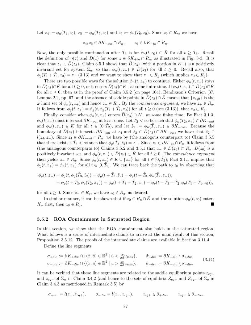
Let z4 := φn(T4, z0), z5 := φn(T5, z0) and z6 := φn(T6, z0). Since z0 ∈ Rn, we have

z4, z5 ∈ ∂K−out ∩Rn, z6 ∈ ∂K−in ∩Rn.

Now, the only possible continuation after T6 is for φn(t, z0) ∈ K for all t ≥ T6. Recallthe definition of η(z) and D(z) for some z ∈ ∂K+in ∩ Rn, as illustrated in Fig. 3-3. It isclear that z+ ∈ D(z3). Claim 3.5.1 shows that D(z3) (with a portion in K−) is a positivelyinvariant set for system Σn, so that φn(t, z+) ∈ D(z3) for all t ≥ 0. Recall also, thatφg(T1 + T1, z0) = z+ (3.13) and we want to show that z+ ∈ Rg (which implies z0 ∈ Rg).

There are two possible ways for the solution φn(t, z+) to continue. Either φn(t, z+) staysin D(z3)∩K for all t ≥ 0, or it enters D(z3)∩K− at some finite time. If φn(t, z+) ∈ D(z3)∩Kfor all t ≥ 0, then as in the proof of Claim 3.5.2 (on page 104), Bendixson’s Criterion [37,Lemma 2.2, pp. 67] and the absence of saddle points in D(z3)∩ K means that zeq0 is theω limit set of φn(t, z+) and hence z+ ∈ Rn. By the coincidence argument, we have z+ ∈ Rg.It follows from φg(t, z+) = φg(t, φg(T1 + T1, z0)) for all t ≥ 0 (see (3.13)), that z0 ∈ Rg.

Finally, consider when φn(t, z+) enters D(z3) ∩K− at some finite time. By Fact 3.1.3,φn(t, z+) must intersect ∂K−out at least once. Let T2 <∞ be such that φn(T2, z+) ∈ ∂K−outand φn(t, z+) ∈ K for all t ∈ (0, T2), and let z2 := φn(T2, z+) ∈ ∂K−out. Because theboundary of D(z3) intersects ∂K−out at z4 and z2 ∈ D(z3) ∩ ∂K−out, we have that z2 ∈l(z4, z−). Since z4 ∈ ∂K−out ∩ Rn, we have by (the analogous counterpart to) Claim 3.5.5that there exists a T3 <∞ such that φg(T3, z2) = z−. Since z6 ∈ ∂K−in∩Rn, it follows from(the analogous counterparts to) Claims 3.5.2 and 3.5.1 that z− ∈ D(z6) ⊂ Rn, D(z6) is apositively invariant set, and φn(t, z−) ∈ D(z6) ⊂ K for all t ≥ 0. The coincidence argumentthen yields z− ∈ Rg. Since φn(t, z+) ∈ K ∪ z+ for all t ∈ [0, T2), Fact 3.1.1 implies thatφg(t, z+) = φn(t, z+) for all t ∈ [0, T2]. We can trace back the path to z0 by observing that

φg(t, z−) = φg(t, φg(T3, z2)) = φg(t+ T3, z2) = φg(t+ T3, φn(T2, z+)),

= φg(t+ T3, φg(T2, z+)) = φg(t+ T3 + T2, z+) = φg(t+ T3 + T2, φg(T1 + T1, z0)),

for all t ≥ 0. Since z− ∈ Rg, we have z0 ∈ Rg, as desired.

In similar manner, it can be shown that if z0 ∈ Rn ∩ K and the solution φn(t, z0) entersK− first, then z0 ∈ Rg.

3.5.2 ROA Containment in Saturated Region

In this section, we show that the ROA containment also holds in the saturated region.What follows is a series of intermediate claims to arrive at the main result of this section,Proposition 3.5.12. The proofs of the intermediate claims are available in Section 3.11.4.

Define the line segments

σ+div := ∂K+div ∩ (x, u) ∈ R2 | u < bcadumax, σ+div := ∂K+div \ σ+div,

σ−div := ∂K−div ∩ (x, u) ∈ R2 | u > bcadumin, σ−div := ∂K−div \ σ−div.

(3.14)

It can be verified that these line segments are related to the saddle equilibrium points zeq+and zeq− of Σn in Claim 3.4.2 (and hence to the sets of equilibria Zeq+ and Zeq− of Σg inClaim 3.4.3 as mentioned in Remark 3.5) by

σ+div = l(z+, zeq+), σ−div = l(z−, zeq−), zeq+ ∈ σ+div, zeq− ∈ σ−div,

87

whenever ad < 0. For the next result, recall the definition of transverse sections, Defini-tion 3.1.

Claim 3.5.8 (Transverse Sections in Saturated Region). If the open-loop system is

(i) marginally stable (a = 0), or strictly stable with a stable controller (a < 0 and d ≤ 0),then ∂K+div is a transverse section to fn;

(ii) strictly stable with an unstable controller (a < 0 and d ∈ (0,−a)), or unstable (a > 0),then σ+div (⊂ ∂K+div) is a transverse section to fn.

Claim 3.5.9. If the open-loop system is

(i) strictly stable with an unstable controller (a < 0 and d ∈ (0,−a)); or(ii) unstable (a > 0);

and z0 ∈ Rn, then z0 6∈ σ+div.

The next result states that when started from the saturated region K+out within theROA of the nominal system, i.e. z0 ∈ K+out ∩Rn, the solution of the GPAW-compensatedsystem will always enter the unsaturated region.

Claim 3.5.10. If z0 ∈ K+out ∩Rn, then there exists a Tn ∈ (0,∞) such that

φn(Tn, z0) ∈ ∂K+in, φn(t, z0) ∈ K+,∀t ∈ [0, Tn). (3.15)

Moreover, there exists a Tg < Tn such that the solution of the GPAW-compensated systemsatisfy

φg(Tg, z0) ∈ l(z+, φn(Tn, z0)) ⊂ ∂K+in.

Remark 3.12. A weaker version of Claim 3.5.10 (where the conclusion is that a Tg ≤ Tnexists such that φg(Tg, z0) ∈ l(z+, φn(Tn, z0)) ∪ φn(Tn, z0)) suffices for the purpose ofproving Proposition 3.5.12. The proof (in pages 109 – 111) would have been shorter, as thecondition ug(t) < un(t) for all t ∈ (0, T ] would be unnecessary. We present this marginallystronger result to confirm the intuitively reasonable conclusion.

The following construction of E(z0) is analogous to the construction of D(z0) in Fig. 3-3.Consider a point z0 ∈ ∂K+in ∩ Rg in the ROA of the GPAW-compensated system. Theo-rem 2.5.3 shows that φg(t, z0) ∈ K for all t ≥ 0. Recall the definition of σ+ (see (3.12)) andlet

tint := inft ∈ (0,∞) | φg(t, z0) ∈ σ+.In other words, tint is the first time instant that the solution of the GPAW-compensatedsystem φg(t, z0) intersects σ+, or ∞ if it does not intersect σ+. Define the path γ(z0) ⊂ R2

by

γ(z0) :=

γintφg(z0) ∪ l(φg(tint, z0), z+) ∪ z+ ∪ l(z0, z+), if tint <∞,γ0φg(z0) ∪ zeq0 ∪ σ+ ∪ l(z0, z+), otherwise,

(3.16)

where

γintφg(z0) := z ∈ R2 | z = φg(t, z0), ∀t ∈ [0, tint],γ0φg(z0) := z ∈ R2 | z = φg(t, z0), ∀t ≥ 0,

88

which can be verified to be closed and connected. Observe that γ(z0) traces the path alongthe solution φg(t, z0) until it intersects σ+ or reach the origin, proceeds along σ+ towardsz+, then along ∂K+in until it reaches its starting point z0. Let the open, bounded regionenclosed by γ(z0) be E(z0), and its closure be E(z0). The region E(z0) is illustrated inFig. 3-4.

x

u

K

K−

E(z0)

γ(z0)

zeq0

z+z0φg(tint, z0)

z−

x

u

K

K−

K+

E(z0)

γ(z0)

zeq0

φg(tint, z0), z+

z0

z−

Figure 3-4: Closed path γ(z0) encloses region E(z0) ⊂ K. A case where the solution intersects∂K−out, then intersects σ+, is shown on the left. A case where the solution intersects∂K+out, then intersects σ+ at z+, is shown on the right.

Remark 3.13. Observe that z+ ∈ σ+. If tint < ∞ and φg(tint, z0) = z+ ∈ σ+, then γ(z0)reduces to γ(z0) = γintφg(z0) ∪ l(z0, z+), since l(φg(tint, z0), z+) = l(z+, z+) = z+ andz+ ∈ γintφg(z0). This case is shown on the right plot of Fig. 3-4. A case analogous tothe preceding is also possible for the path η(z0) in Fig. 3-3. However, it happens onlyfor a single trajectory (if it exists). The peculiar nature of φg(t, z0) implied by controllerstate-output consistency (Theorem 2.5.3) means that this case happens whenever φg(t, z0)intersects ∂K+out and slides along it to reach z+.

The following result in analogous to Claims 3.5.1 and 3.5.2 combined, with respect toE(z0).

Claim 3.5.11 (Invariance of E(z0) ⊂ Rg). If z0 ∈ ∂K+in ∩ Rg, then E(z0) ⊂ K is apositively invariant set for system Σg. Moreover, E(z0) is contained in the ROA of systemΣg, and it must contain zeq0, i.e. zeq0 ∈ E(z0) ⊂ Rg.

The following is the main result of this section.

Proposition 3.5.12 (ROA Containment in Saturated Region). The part of the ROA ofthe origin of system Σn contained in R2 \K, is itself contained within the ROA of the originof system Σg, i.e. (Rn ∩ (R2 \ K)) ⊂ Rg.

Proof. We need to show that if z0 ∈ Rn ∩ (R2 \ K), then z0 ∈ Rg. First, observe thatR2 \ K = K+ ∪K−, and K+ = K+out ∪K+in ∪ ∂K+div. We will show that if z0 ∈ Rn ∩K+,then z0 ∈ Rg. The proof where z0 ∈ Rn ∩K− is similar. Let z0 ∈ Rn ∩K+. Since z0 ∈ Rnand zeq0 ∈ K, Fact 3.1.2 shows that φn(t, z0) must intersect ∂K+in at least once. Let Tbe the first time instant that φn(t, z0) intersects ∂K+in, so that φn(T, z0) ∈ ∂K+in andφn(t, z0) ∈ K+ for all t ∈ [0, T ).

89

Consider when z0 ∈ Rn ∩ (K+in ∪ ∂K+div) ⊂ Rn ∩K+. We claim that φn(t, z0) must becontained in K+in ∪ ∂K+div (and hence cannot enter K+out) for all t ∈ [0, T ). Otherwise,φn(t, z0) must intersect ∂K+div at some finite time T ∈ (0, T ) and then pass into K+out.Claims 3.5.8 and 3.5.9 show that φn(t, z0) must pass through ∂K+div or σ+div, which aretransverse sections. By similar reasoning as in the proof of Claim 3.5.10 (on pages 109 –111), φn(t, z0) can never return to K+in during the interval [T , T ]. In that case, φn(t, z0)can never intersect ∂K+in at t = T , which is a contradiction that establishes the immediateclaim.

Since φn(t, z0) ∈ K+in ∪ ∂K+div for all t ∈ [0, T ), Fact 3.1.1 yields φg(t, z0) = φn(t, z0)for all t ∈ [0, T ]. Since z0 ∈ Rn, we have φn(T, z0) = φg(T, z0) ∈ Rn ∩ ∂K+in ⊂ Rn ∩ K.Proposition 3.5.7 then shows that φg(T, z0) ∈ Rg, so that z0 ∈ Rg, as desired.

Next, consider when z0 ∈ Rn ∩ K+out ⊂ Rn ∩ K+. Claim 3.5.10 shows that thereexists a Tg ∈ (0, T ) such that φg(Tg, z0) ∈ l(z+, φn(T, z0)) ⊂ ∂K+in. Since z0 ∈ Rn andφn(T, z0) ∈ ∂K+in, we have φn(T, z0) ∈ Rn ∩ ∂K+in ⊂ Rn ∩ K. Proposition 3.5.7 thenshows that φn(T, z0) ∈ Rg. Observing that φn(T, z0) ∈ ∂K+in ∩ Rg, Claim 3.5.11 showsthat l(z+, φn(T, z0)) ⊂ E(φn(T, z0)) ⊂ Rg. Then φg(Tg, z0) ∈ l(z+, φn(T, z0)) ⊂ Rg impliesz0 ∈ Rg, as desired.

Finally, by observing that (Rn ∩ (K+in ∪ ∂K+div)) ∪ (Rn ∩ K+out) = Rn ∩ K+, theconclusion follows.

3.5.3 Main Result

The following is the main result of this chapter, which shows that the GPAW scheme canonly maintain/enlarge the ROA of the uncompensated system. This shows that the GPAWscheme satisfies condition (i) of the general anti-windup problem (Problem 1 in Section 1.3).

Proposition 3.5.13 (ROA Containment). The ROA of the origin of system Σn is containedwithin the ROA of the origin of system Σg, i.e. Rn ⊂ Rg.Proof. Propositions 3.5.7 and 3.5.12 gives

(Rn ∩ K) ⊂ Rg, (Rn ∩ (R2 \ K)) ⊂ Rg,

respectively. The conclusion follows by taking the respective unions of both the left andright sides in the preceding, which gives

Rn = ((Rn ∩ K) ∪ (Rn ∩ (R2 \ K))) ⊂ (Rg ∪Rg) = Rg.

Remark 3.14. Observe that Proposition 3.5.13 is a strong result. It implies that for everyLyapunov function Vn(z) that certifies an ROA Rn ⊂ Rn for the nominal system Σn,there exists a Lyapunov function Vg(z) (possibly Vg(z) ≡ Vn(z)) that certifies an ROARg for the GPAW-compensated system Σg satisfying Rn ⊂ Rg ⊂ Rg. This is in contrastto conventional Lyapunov analysis that seeks a single non-unique Lyapunov function. Inparticular, this result implies that if there exists a Lyapunov function that certifies globalasymptotic stability for the origin of the nominal system, i.e. Rn = R2, then there existsa Lyapunov function that also certifies global asymptotic stability for the origin of theGPAW-compensated system, i.e. (Rg ⊃ Rn = R2)⇒ (Rg = R2). See Corollary 3.7.2 for anexample application.

Remark 3.15. While Proposition 3.5.13 does not provide an estimate of the ROA, it can beestimated by numerous known methods, e.g. see [155–166]. We consider the estimation of

90

ROAs as a separate problem that need not be associated with the anti-windup problem, incontrast to [14].

3.5.4 Numerical Results

Here, we present some numerical results on the exact ROAs of systems Σn and Σg. As willbe shown in Section 3.6, these results also indicate that asymmetric saturation constraintsshould be considered for any anti-windup scheme to be practically useful. The ROAs inthese figures (Fig. 3-5, Fig. 3-6, and Fig. 3-7) are to be interpreted as open sets, since ROAsmust be open [37, Lemma 8.1, p. 314].

−2.5 −2 −1.5 −1 −0.5 0 0.5 1 1.5 2 2.5−5

−4

−3

−2

−1

0

1

2

3

4

5

x

u Rn = Rg

φn(t, z0)

φg(t, z0)

(a) symmetric constraints, umax = −umin.

−2.5 −2 −1.5 −1 −0.5 0 0.5 1 1.5 2 2.5−5

−4

−3

−2

−1

0

1

2

3

4

5

x

u

Rn

Rg

φn(t, z0)

φg(t, z0)

(b) asymmetric constraints, umax > −umin.

Figure 3-5: Region of attraction (ROA) containment for system with open-loop unstable plant (pa-rameters: a = 1, b = 1, c = −3, d = −1.2). The vector field fn is shown in thebackground, light purple regions represent Rn (⊂ Rg), and light blue regions representRg \ Rn. In (a), the saturation limits are symmetric (umax = −umin = 1), result-ing in Rn = Rg. Two pairs of solutions starting at z0 = (0.85,−4) ∈ Rn ∩ Rg andz0 = (−0.66, 4) 6∈ Rn ∪ Rg are included. In (b), the ROA containment Rn ⊂ Rg ofProposition 3.5.13 holds strictly. The system is identical with the one in (a), exceptwith asymmetric saturation limits (umax = 1.5 > −umin = 1). Two pairs of solutionsstarting from z0 = (0.9,−1.9) ∈ Rn ∩Rg and z0 = (0.37,−4.37) ∈ Rg \Rn are included.

Fig. 3-5(a) shows the case where Rn = Rg for a system with an open-loop unstableplant, together with two pairs of representative solutions, when the saturation constraintsare symmetric, i.e. umax = −umin. When the same system is subjected to asymmetricsaturation constraints, the ROAs are illustrated in Fig. 3-5(b). Clearly, the set containmentRn ⊂ Rg result of Proposition 3.5.13 holds strictly. In Fig. 3-6, the ROAs are illustratedfor a system with an open-loop stable plant and an unstable controller (a < 0 < d < −a).Again, the set containment Rn ⊂ Rg is strict.

Remark 3.16. Note that the case of asymmetric saturation constraints is not pathological.Even with actuators having symmetric saturation constraints, it arises when regulatingabout an equilibrium point not lying in (x, u) ∈ R2 | u = 0, and the system state istransformed such that the resulting equilibrium lies at the origin.

Remark 3.17. Observe from Fig. 3-6 that if we force the initial controller state to satisfyu(0) = sat(u(0)), e.g. by initializing the controller state to be u(0) = sat(u0) for any given

91

−5 −4 −3 −2 −1 0 1 2 3 4 5−3

−2

−1

0

1

2

3

x

u

Rn

Rg

φn(t, z0)

φg(t, z0)

Figure 3-6: Region of attraction (ROA) containment for system with open-loop stable plant (pa-rameters: a = −1, b = 1, c = −1, d = 0.5, umax = −umin = 1), which shows the ROAcontainment Rn ⊂ Rg of Proposition 3.5.13 can hold strictly. The vector field fn is shownin the background, light purple regions represent Rn (⊂ Rg), and light blue regions rep-resent Rg \Rn. Two pairs of solutions starting from z0 = (−3.7,−2.54) ∈ Rn ∩Rg andz0 = (4, 1.6) ∈ Rg \Rn are included.

nominal initialization u0, then the effective ROA

Rge := (x, u) ∈ R2 | z0 = (x, sat(u)), φg(t, z0)→ zeq0 as t→∞,

would be the entire state space, i.e. Rge = R2, achieving global asymptotic stability for thiscase.

Assumption 3.1 restricts the possible qualitative characteristics of the nominal controller.When the open-loop plant is unstable, i.e. a > 0, condition (3.6) restricts the nominalcontroller to be strictly stable, i.e. d < −a < 0. This case is covered in Fig. 3-5. When theopen-loop plant is marginally or strictly stable, i.e. a ≤ 0, the nominal controller can beeither stable or unstable as long as d < −a (due to condition (3.6)). The case of unstablenominal controllers, i.e. 0 < d < −a is covered in Fig. 3-6. The case where both theopen-loop plant and nominal controller are marginally or strictly stable will be discussed inSection 3.7.

3.6 Illustration of the Need to Consider Asymmetric Satu-ration Constraints

The main purpose of the numerical results in Section 3.5.4 is to validate the ROA contain-ment result Rn ⊂ Rg of Proposition 3.5.13. Here, we discuss further implications of theseresults, and show the need to consider asymmetric saturation constraints for analysis ofgeneral input-constrained systems (see also Remark 3.16).

First, consider the following intuitively appealing statement.

Statement 3.1 (Relaxed Constraints Imply ROA Enlargement). Consider a closed-loopautonomous system Σaut defined by the feedback interconnection of a saturated open-loopsystem and some controller. Let Raut1 be the ROA of some equilibrium point zeq of systemΣaut corresponding to some saturation limits umin1,i, umax1,i (see (1.2)) satisfying umin1,i <

92

umax1,i for all i ∈ 1, 2, . . . ,m, where m is the dimension of the control input. If someumin2,i, umax2,i are such that

umin2,i ≤ umin1,i < umax1,i ≤ umax2,i, ∀i ∈ 1, 2, . . . ,m,

then the ROA Raut2 of zeq of system Σaut corresponding to these relaxed saturation limits,umin2,i, umax2,i, must contain Raut1, i.e. Raut1 ⊂ Raut2.

Statement 3.1 suggests that relaxing the saturation constraints can only enlarge theassociated ROA, and appeals to the intuitive notion that “things cannot get worse if welessen the contributing factors that led to the original performance/stability problems”. IfStatement 3.1 is true, then analysis of saturated feedback systems reduces to the analysiswith the worst case saturation constraints (under perturbations) and provides a significantamount of simplifications. While there is evidence to suggest the truth of Statement 3.1when the open-loop plant is not unstable (provided the controller is appropriately designed),the ROA results in Fig. 3-7 shows Statement 3.1 to be false in general, in particular whenthe open-loop plant is unstable. The ROAs shown in Fig. 3-7 are identical to those in

−2.5 −2 −1.5 −1 −0.5 0 0.5 1 1.5 2 2.5−5

−4

−3

−2

−1

0

1

2

3

4

5

x

u Rn = Rg

φn(t, z0)

φg(t, z0)

(a) symmetric constraints, umax = −umin.

−2.5 −2 −1.5 −1 −0.5 0 0.5 1 1.5 2 2.5−5

−4

−3

−2

−1

0

1

2

3

4

5

x

u

Rn

Rg

φn(t, z0)

φg(t, z0)

(b) asymmetric constraints, umax > −umin.

Figure 3-7: Illustrating the need to consider asymmetric saturation constraints. The ROAs shownare identical to those in Fig. 3-5. In the left plot where the system is with symmetricsaturation constraints (umax = −umin = 1), the point z0 = (−0.8, 2.5) lies in bothROAs, i.e. z0 ∈ Rn ∩Rg. In the right plot representing an identical system with relaxedbut asymmetric saturation constraints (umax = 1.5 > −umin = 1), the same point liesoutside both ROAs, i.e. z0 6∈ Rn ∪Rg.

Fig. 3-5, but with only a single pair of solutions starting from the point z0 = (−0.8, 2.5). Asbefore, Fig. 3-7(b) shows the ROAs associated with a system identical to that in Fig. 3-7(a),except with relaxed but asymmetric saturation limits umax 6= −umin. It can be seen fromFig. 3-7(a) that with the original (symmetric) saturation limits, the point z0 lies in both theROAs of systems Σn and Σg. With the relaxed saturation limits, the point z0 lies outside theROAs of both systems Σn and Σg. Hence any sufficiently “tight” ROA estimate9 obtainedwith symmetric saturation limits becomes invalid with asymmetric saturation limits, evenwhen they are relaxed.

9By a “tight” ROA estimate, we mean one that is close to the exact ROA.

93

The vast majority of literature on input-constrained systems, including the anti-windupliterature, consider only symmetric saturation constraints. One exception is [47], which ismotivated by the fact that results obtained by the same authors for the symmetric saturationcase do not carry over to the asymmetric saturation case. These results indicate a dire needto consider asymmetric saturation constraints for practical utility.

3.7 A Paradigm Shift in Anti-windup Compensation

Here, we propose a new way of addressing the general anti-windup problem, which hasbeen reflected in the statement of Problem 1 (in Section 1.3) as conditions (i) and (iii). Toaid in the subsequent discussion, we present the next result, which states that the nominaluncompensated system achieves global asymptotic stability (GAS) and local exponentialstability (LES) when both the open-loop plant and nominal controller are marginally orstrictly stable.

Claim 3.7.1 (Global Asymptotic Stability of Nominal System). If in addition to Assump-tion 3.1, both the open-loop plant and nominal controller are marginally or strictly stable(a ≤ 0 and d ≤ 0), then the origin zeq0 of the nominal system Σn is globally asymptoticallystable and locally exponentially stable.

Remark 3.18. This is the main reason why this case is not considered in Section 3.5.4.

Proof. The proof follows [38, Example 3.14, pp. 74 – 75] closely. First, the nominal systemΣn (3.4) is governed by the ODEs

x = ax+ b sat(u),

u = cx+ du,

which can be rewritten as

u = cx+ du = c(ax+ b sat(u)) + du = a(u− du) + bc sat(u) + du,

= (a+ d)u− adu+ bc sat(u). (3.17)

Consider the continuously differentiable function

V (u, u) = 12 u

2 + V (u), V (u) :=

∫ u

0(adτ − bc sat(τ)) dτ.

We will show that V (u, u) is positive definite when ad ≥ 0, which is implied by the assump-tion a ≤ 0 and d ≤ 0. Clearly, it is sufficient to show that V (u) is positive definite. Whenumin ≤ u ≤ umax, we have sat(u) = u, and

V (u) =

∫ u

0(ad− bc)τ dτ = 1

2(ad− bc)u2,

so that from (3.7), V (u) > 0 for all u ∈ [umin, umax] \ 0. Next, consider when u =

94

u+ umax > umax for some u > 0. Direct computation yields

V (u) = 12adu

2 −∫ umax

0bcτ dτ −

∫ u

umax

bcumax dτ,

= 12adu

2 − 12bcu

2max − bcuumax,

= 12ad(u2 + 2uumax + u2

max)− 12bcu

2max − bcuumax,

= 12adu

2 + (ad− bc)uumax + 12(ad− bc)u2

max.

Clearly, when ad ≥ 0, (3.7) implies V (u) > 0 for all u > umax. The case when u < umin

can be shown similarly. Hence V (u, u) is positive definite. The above expressions also showthat V (u, u) is radially unbounded.

Taking the time derivative of V (u, u) and using (3.17) yields

V (u, u) = uu+ (adu− bc sat(u))u = u((a+ d)u− adu+ bc sat(u)) + (adu− bc sat(u))u,

= (a+ d)u2.

Condition (3.6) then shows V (u, u) to be negative semidefinite, i.e. V (u, u) ≤ 0.

To complete the proof for global asymptotic stability, it is sufficient to show thatV (u, u) ≡ 0 implies u ≡ 0 and u ≡ 0. The first condition is obtained immediately dueto (3.6) (specifically, a+ d 6= 0). When u ≡ 0, (3.17) reduces to

u = −adu+ bc sat(u),

so that by (3.7), u 6= 0 as long as u 6= 0. Hence only the trivial solution u ≡ 0, u ≡ 0 canstay identically in the set S = (u, u) ∈ R2 | V (u, u) = 0. By [37, Corollary 4.2, p. 129],the origin of Σn is globally asymptotically stable. Local exponential stability of the originfollows immediately from Assumption 3.1.

Remark 3.19. Observe that (3.6) precludes ad ≥ 0 being satisfied when either the open-loopplant or nominal controller is unstable, i.e. a > 0 or d > 0.

Corollary 3.7.2 (Global Asymptotic Stability of GPAW-Compensated System). If in ad-dition to Assumption 3.1, both the open-loop plant and nominal controller are marginallyor strictly stable (a ≤ 0 and d ≤ 0), then the origin zeq0 of the GPAW-compensated systemΣg is globally asymptotically stable and locally exponentially stable.

Proof. Claim 3.7.1 shows that the origin zeq0 is globally asymptotically stable for system Σn,which implies Rn = R2. Proposition 3.5.13 then yields Rg ⊃ Rn = R2, which implies Rg =R2 and the origin zeq0 is globally asymptotically stable for system Σg. Local exponentialstability of the origin follows immediately from Assumption 3.1.

Numerous results in the anti-windup literature are of the form of Corollary 3.7.2, i.e. un-der some assumptions and applying some anti-windup method, some stability properties areachieved. Such results sound impressive, and may indeed give some confidence in the ap-plication of the particular anti-windup method. However, we argue that it may not revealany advantages of the anti-windup method. First, observe that for any meaningful anti-windup problem, local stability must be assumed. Otherwise, the anti-windup problem isill-posed. Any results asserting local stability are only restating the assumption. Observefrom Claim 3.7.1 that the uncompensated nominal system achieves GAS. In other words,

95

GAS is achieved without any anti-windup compensation. While Corollary 3.7.2 asserts GAS,it tells nothing of any advantages gained by adopting the particular anti-windup method.

In contrast, the ROA containment result of Proposition 3.5.13 truly reflects an advan-tage of the GPAW scheme, namely, that the ROA of the system will always be main-tained/enlarged by its application. As such, we propose this new paradigm to addressthe anti-windup problem, i.e. results on the anti-windup compensated system relative tothe uncompensated system. This is reflected as conditions (i) and (iii) of Problem 1 (inSection 1.3).

3.8 Relation to the General Anti-windup Problem

Here, we discuss how the obtained results for the GPAW scheme relate to the general anti-windup problem (Problem 1 of Section 1.3) for the nominal system (3.4). First, observethat condition (i) of Problem 1 is fulfilled by the GPAW scheme due to Proposition 3.5.13.Condition (ii) is fulfilled by construction (see Remark 2.17 and item (ii) of the concludingobservations in Section 2.5 on page 52). Numerous performance metrics can be specifiedto show that application of GPAW compensation on system (3.4) will maintain/improveperformance, hence fulfilling condition (iii) of Problem 1. However, this is non-trivial (seeRemark 3.20), and similar arguments as in the proofs of Propositions 3.5.7 and 3.5.12 wouldbe involved in general.

For an informal discussion, consider the L2 norm [41, p. 2] of the state10

J = ‖z‖2 = ‖(x, u)‖2 :=

(∫ ∞0

V (x(t), u(t)) dt

) 12

, V (z) := V (x, u) := x2 + u2, (3.18)

with a lower J indicating greater performance. Let the performance attained by systemsΣg and Σn be

Jg =

(∫ ∞0

V (xg(t), ug(t)) dt

) 12

, Jn =

(∫ ∞0

V (xn(t), un(t)) dt

) 12

,

respectively, where (xg(t), ug(t)) = φg(t, z0) and (xn(t), un(t)) = φn(t, z0) are their respec-tive solutions. The function V (x, u) is the square of the magnitude of the state from theorigin. It can be seen from Figs. 3-5, 3-6, and 3-7, that when started from the same pointz0, the state of the GPAW-compensated system Σg for these cases are in some sense smallerin magnitude than the state of the nominal system Σn, so that Jg ≤ Jn likely holds. Weleave the actual proofs as future work (see Section 7.1.8).

Remark 3.20. It can be shown that for V (z) as defined in (3.18),

∂V (z)

∂zfg(z) ≤

∂V (z)

∂zfn(z), ∀z ∈ R2,

holds, where fg and fn are the vector fields of the GPAW-compensated system Σg (3.5)and nominal system Σn (3.4) respectively. We note that this is not a sufficient condition to

10Note that the use of the L2 performance measure differs from that in [14]. Moreover, the finite L2 gainperformance measure in [14] is not meaningful for autonomous systems that are not driven by any exogenousinputs.

96

show that V (xg(t), ug(t)) ≤ V (xn(t), un(t)) for all t ≥ 0. However, if

∂V (φg(t, z0))

∂zfg(φg(t, z0)) ≤ ∂V (φn(t, z0))

∂zfn(φn(t, z0)), ∀t ≥ 0,∀z0 ∈ R2,

holds, then V (φg(t, z0)) = V (xg(t), ug(t)) ≤ V (xn(t), un(t)) = V (φn(t, z0)) for all t ≥ 0follows easily, which implies Jg ≤ Jn. The need to evaluation the function V (z) along twodifferent trajectories renders it a non-trivial task.

In summary, when GPAW compensation is applied to the nominal system (3.4), (i) nom-inal performance is recovered whenever no controls saturate; and (ii) stability is nevercompromised. Observe that these are achieved for all plant and controller parameters(a, b, c, d, umax, umin) with umin < umax and (a, b, c, d) satisfying the standard anti-windupassumption (Assumption 3.1).

3.9 Solution Bounce Property and Some Conjectures

Here, we show that the solution of the GPAW-compensated system Σg can bounce (definedmore concretely in Definition 3.3 below) on the saturation constraint boundaries ∂K+ and∂K− at most once. This indicates the possible existence of some optimality properties,which we state as a conjecture. Further optimality conjectures are also presented, theverification of which we leave as future work (see Section 7.1.8). First, we define a solutionbounce.

Definition 3.3 (Solution Bounce). A solution φ(t, z0) is said to bounce on the saturationconstraint boundary ∂K+ (3.8) if there exists an ε > 0 and an interval [t1, t2], t1 ≤ t2, suchthat

φ(t, z0) ∈ (∂K+ ∪K+), ∀t ∈ [t1, t2],

φ(t, z0) ∈ K, ∀t ∈ [t1 − ε, t1) ∪ (t2, t2 + ε],

with an analogous counterpart for the saturation constraint boundary ∂K−.

In other words, a solution bounce is an event where the solution starting from the interiorof the unsaturated region K enters the region R2 \K (which contains the saturated regionK+ ∪ K− and constraint boundaries ∂K+ ∪ ∂K−) for some finite interval (or single timeinstant when t1 = t2), and returns to the interior K thereafter. Observe that Definition 3.3excludes those instances where the solution starts from R2 \K and enters K. If t1 = t2 inDefinition 3.3, the solution intersects the saturation constraint boundary only at a singlepoint in time.

The following gives an upper bound on the number of solution bounces for the GPAW-compensated system Σg. This property depends critically on the controller state-outputconsistency property (Theorem 2.5.3) unique to the GPAW scheme.

Proposition 3.9.1 (Upper Bound on Number of Solution Bounces for Σg). For all z0 ∈ Rg,the solution of the GPAW-compensated system φg(t, z0) can have at most one bounce eachon ∂K+ and ∂K−.

Proof. We will prove the case when the solution bounces on ∂K+. The proof when thesolution bounces on ∂K− is similar. Assume for the sake of contradiction that for some

97

z0 ∈ Rg, the solution φg(t, z0) has two or more bounces on ∂K+. Then there exists ε1 > 0,ε2 > 0, and two intervals [t1, t2], [t3, t4] such that

φg(t, z0) ∈ (∂K+ ∪K+), ∀t ∈ [t1, t2] ∪ [t3, t4],

φg(t, z0) ∈ K, ∀t ∈ [t1 − ε1, t1) ∪ (t2, t2 + ε1],

φg(t, z0) ∈ K, ∀t ∈ [t3 − ε2, t3) ∪ (t4, t4 + ε2].

Observing that K ∩ (∂K+ ∪ K+) = ∅ (see (3.8)), the preceding implies either t2 < t3 ort4 < t1. Without loss of generality, assume that t2 < t3. From the definitions of fg (3.5) and∂K+out (3.8), the point where the solution leaves ∂K+ must lie in ∂K+\∂K+out = (∂K+in∪z+), i.e. φg(t2, z0), φg(t4, z0) ∈ ∂K+in ∪ z+. Theorem 2.5.3 shows that φg(t, z0) 6∈ K+

for all t ∈ [t1, t2] ∪ [t3, t4], which, together with Fact 3.1.2 shows that the solution cannotleave ∂K+ ∪K+ through ∂K+in. Hence φg(t2, z0) = φg(t4, z0) = z+. The solution in theinterval [t2, t4] then forms a closed orbit, γ = z ∈ R2 | z = φg(t, z0), ∀t ∈ [t2, t4]. By theuniqueness of solutions (see Proposition 3.3.3 and Remark 3.3), we have φg(t, z0) ∈ γ forall t ≥ t4 and limt→∞ φg(t, z0) 6= zeq0. Hence z0 6∈ Rg, a contradiction.

Remark 3.21. It is clear from the proof that if the solution φg(t, z0) intersects ∂K+ at asingle point in time, then it must intersect it at z+. This is also clear from the definitionsof ∂K+out, ∂K+in, and z+ in (3.8).

Proposition 3.9.1 suggests an intuitively clear optimality property of the GPAW-compensatedsystem, namely that for system Σn, the GPAW scheme achieves the minimal number ofsolution bounces. In other words, no other anti-windup schemes can do better. We statethis below, whose proof we leave as future work (see Section 7.1.8).

Conjecture 3.1 (Optimality in Number of Solution Bounces). The GPAW scheme appliedto system Σn (3.4) is an optimal anti-windup scheme achieving the least number of solutionbounces on ∂K+ and ∂K− for all initial conditions in the ROA of the uncompensatedsystem Σn, i.e. for all z0 ∈ Rn.

Remark 3.22. We have stated the conjecture in terms of initial conditions in the ROA ofthe nominal system to provide a fair basis of comparison. Different anti-windup schemesmay achieve different ROAs, but they all must contain Rn according to our criterion fora valid anti-windup scheme. Let Raw1, Raw2 and φaw1(t, z0), φaw2(t, z0) be the ROAs andsolutions corresponding to two different anti-windup compensated (closed-loop) systems. If∂K+ ∩ Raw1 = ∅ and ∂K+ ∩ Raw2 6= ∅, then φaw1(t, z0) may not bounce (it may tend toinfinity without returning to K), while φaw2(t, z0) will bounce, if started at a point withinRaw2 \ Raw1 sufficiently close to ∂K+. However, this would not be a fair comparison, andhence the restriction to initial conditions within Rn ⊂ (Raw1 ∩Raw2).

To see that Conjecture 3.1 is at least plausible, assume that z0 ∈ K∩Rn is such that thenominal solution φn(t, z0) will intersect ∂K+ at some time. Let φaw(t, z0) be the solutionof some anti-windup compensated system, which must satisfy φaw(t, z0) = φn(t, z0) for allt such that φn(t, z0) ∈ K (to recover nominal performance in the absence of saturation).Hence φaw(t, z0) must bounce on ∂K+ at least once, which is the maximum achieved byGPAW compensation due to Proposition 3.9.1. This is sufficient to prove Conjecture 3.1 ifthe anti-windup compensated system is second order. To prove the conjecture, we need toshow this for anti-windup compensated systems of arbitrary (finite) order, e.g. when usingdynamic anti-windup schemes, which we leave as future work (see Section 7.1.8).

The next conjecture is motivated by Proposition 3.5.13, Fig. 3-6, and Remark 3.17.

98

Conjecture 3.2 (Optimality in ROA). Consider the GPAW scheme applied to systemΣn (3.4) with the controller state initialization u(0) = sat(u0), where u0 is some nominalinitialization. The effective ROA of this GPAW-compensated system defined by

Rgi := (x, u) ∈ R2 | z0 = (x, sat(u)), φg(t, z0)→ zeq0 as t→∞,

is the largest possible ROA for any anti-windup scheme. In other words, the GPAW schemewith this initialization is an optimal anti-windup scheme achieving the largest ROA.

The conjecture states that if Raw is the achieved ROA for some anti-windup scheme,then Raw ⊂ Rgi. To see that this is at least plausible, let Σaw and Raw be the anti-windup compensated system and ROA obtained by some anti-windup scheme. Now, letΣgi and Rgi be the system and ROA obtained by applying GPAW compensation on Σaw

(with the controller state initialization u(0) = sat(u0)). Proposition 3.5.13 then yieldsRaw ⊂ Rgi. Now, observe that any anti-windup scheme can modify the nominal vector fieldfn only in the saturated region K+ ∪K− ∪ ∂K+ ∪ ∂K− due to the necessity of recoveringnominal performance in the absence of saturation. With the controller state initializationu(0) = sat(u0), all solutions of Σgi starts within the unsaturated region. Hence only thepart of the vector field fg within the unsaturated region K is of concern. Moreover, theGPAW scheme overrides any modification of the nominal vector field on the saturationconstraint boundaries ∂K+ ∪ ∂K−, cancelling any effect of the prior anti-windup scheme.Note that if some anti-windup scheme is applied on the GPAW-compensated controller anddriven by the signal sat(u)− u, then it will be disabled. This is due to u(0) = sat(u0) andTheorem 2.5.3, yielding sat(u)− u ≡ 0 (see also Remark 2.21).

The preceding is a plausibility argument for comparing the GPAW scheme against an-other anti-windup method. To prove the conjecture, we first need to show that the controllerstate initialization u(0) = sat(u0) forcing the state to the unsaturated region, will not induceinstability, i.e. if (x0, u0) ∈ Rg, then (x0, sat(u0)) ∈ Rg. The comparison against dynamicanti-windup schemes is also necessary to prove Conjecture 3.2. This will involve definingsome ways to compare ROAs in different dimensions. For example, in Rn, we can definethe ROA of the second order GPAW-compensated system as Rgi×Rn−2 for the purpose ofROA comparison.

3.10 Chapter Summary

We applied the GPAW scheme to a first order input-constrained LTI plant driven by a firstorder LTI controller, where the objective is to regulate the system state about the origin.Existence and uniqueness of solutions to the GPAW-compensated system are assured usingresults from the projected dynamical systems literature, and equilibria are characterized.The main result of this chapter is that GPAW compensation applied to this simple systemcan only maintain/enlarge the system’s region of attraction. Numerical results indicate aneed to consider asymmetric saturation constraints for general input-constrained systems.The weaknesses of some qualitative results on anti-windup methods are illustrated, whichmotivated a new paradigm for addressing the anti-windup problem. We discuss how theresults in this chapter relate to the general anti-windup problem (Problem 1 of Section 1.3),and presented the solution bounce property together with some conjectures.

The results in this chapter, while limited in applicability, reveals some attractive featuresof the GPAW scheme when restricted to this simple system. These results are strong, and are

99

valid for all plant and controller parameters satisfying the standard anti-windup assumptionof unconstrained nominal stability. In the remainder of this dissertation, we develop toolsto enable the extension of these results to more general plants and/or controllers.

3.11 Chapter Supplement

Here, we collect some supplementary material for this chapter. The strict ComparisonLemma presented in Section 3.11.2 may be of general interest.

3.11.1 Translating Some Logical Statements

In some of the proofs in this chapter, e.g. Claim 3.5.4, we need to assert the truth ofstatements of the form

“if z ∈ α and z ∈ β, then z ∈ γ”. (3.19)

Here, we show explicitly that this statement is equivalent to

“if z ∈ α \ γ, then z 6∈ β”. (3.20)

Note that ¬, ∧, ∨, ⇒, and ⇔, represent logical negation (NOT operator), conjunction(AND operator), disjunction (OR operator), implication, and equivalence respectively. Let

A⇔ (z ∈ α), B ⇔ (z ∈ β), C ⇔ (z ∈ γ),

so that the original statement (3.19) is equivalent to (A ∧ B) ⇒ C. Using the equivalence(A⇒ B)⇔ (¬A ∨B) [167, Fig. 7.11, p. 210], the preceding can be rewritten as

(A ∧B)⇒ C ⇔ ¬(A ∧B) ∨ C ⇔ ¬A ∨ ¬B ∨ C ⇔ ¬A ∨ C ∨ ¬B,⇔ ¬(A ∧ ¬C) ∨ ¬B ⇔ (A ∧ ¬C)⇒ ¬B.

In other words, the original statement is equivalent to

“if z ∈ α and z 6∈ γ, then z 6∈ β”,

or more compactly as (3.20).

Moreover, observe that we can always replace A by more complex statements to get ananalogous equivalence relation. For example, if A⇔ (D ∨ E) ∧ F , then

((D ∨ E) ∧ F ∧B ⇒ C)⇔ ((D ∨ E) ∧ F ∧ ¬C ⇒ ¬B).

In fact, the more complex form is encountered more often.

3.11.2 A Variant of the Comparison Lemma

Here, we present a variant of the Comparison Lemma [37, Lemma 3.4, pp. 102 – 103],where the conclusion results in a strict inequality. It is a direct consequence of uniqueness ofsolutions of the scalar differential equation, with an application of the original ComparisonLemma.

100

Lemma 3.11.1 (Strict Comparison Lemma). Consider the scalar differential equation

u = f(t, u), u(t0) = u0, (3.21)

where f(t, u) is continuous in t and locally Lipschitz in u, for all t ≥ t0 and all u ∈ J ⊂ R,and where J is a connected interval. Let [t0, T ) (T could be infinity) be the maximalinterval of existence of the solution u(t), and suppose u(t) ∈ J for all t ∈ [t0, T ). Let v(t)be a continuous function whose upper right-hand derivative D+v(t) satisfies the differentialinequality

D+v(t) ≤ f(t, v(t)), v(t0) < v0, (3.22)

where v(t) ∈ J for all t ∈ [t0, T ). Then v(t) < u(t) holds for all t ∈ [t0, T ).

Remark 3.23. Observe that the fundamental qualitative difference with [37, Lemma 3.4,pp. 102 – 103] is the strict inequality of the initial condition v(t0) < u0, and the conclusionv(t) < u(t) for all t ∈ [t0, T ). The requirement of J being connected is purely technical, asseen in the proof. See also [37, Appendix C.2, pp. 659 – 660] for a definition of the upperright-hand derivative D+v(t).

Proof. Consider the initial value problem

w = f(t, w), w(t0) = v(t0) < u0. (3.23)

With the assumptions, [37, Theorem 3.1, pp. 88 – 89] implies existence and uniquenessof solutions of (3.21) and (3.23). Let [t0, Tw) be the maximal interval of existence of thesolution w(t) such that w(t) ∈ J for all t ∈ [t0, Tw). Define T := minT, Tw.

We claim that w(t) 6= u(t) for all t ∈ [t0, T ) (due to w(t0) 6= u(t0)). Otherwise, thereexists a T ∈ [t0, T ) such that w(T ) = u(T ). By solving (3.21) and (3.23) backwards intime from t = T to t = t0, we obtain w(t0) = u(t0) due to uniqueness of solutions. Thiscontradicts w(t0) 6= u(t0) and establishes the claim.

Since w(t0) < u(t0), and w(t) 6= u(t) for all t ∈ [t0, T ), continuity of both w(t) andu(t) shows that w(t) < u(t) holds with strict inequality for all t ∈ [t0, T ). The ComparisonLemma [37, Lemma 3.4, pp. 102 – 103] applied to (3.23) and the differential inequality (3.22)yields v(t) ≤ w(t) for all t ∈ [t0, T ). Then we have v(t) ≤ w(t) < u(t) for all t ∈ [t0, T ).This, together with the connectivity of J and the condition u(t), v(t) ∈ J for all t ∈ [t0, T )implies w(t) ∈ J for all t ∈ [t0, T ), i.e. Tw ≥ T and T = T . Hence the conclusion v(t) < u(t)holds with strict inequality for all t ∈ [t0, T ).

3.11.3 Proofs of Intermediate Results for Section 3.5.1

Proof of Claim 3.5.1 (Invariance of D(z0))

Let

σ+ :=

l(φn(tint, z0), z+) ∪ z+, if tint <∞,σ+, otherwise.

We first show that σ+ is a transverse section to fn, and that fn always points into D(z0) onσ+. Let α ∈ −1,+1 be chosen such that 〈αTz+, z0−z+〉 > 0, where T z+ := (umax,

dcumax)

is orthogonal to z+ (see (3.8)). Then αT z+‖z+‖ is the unit normal of σ+ that points into

D(z0). Hence σ+ is a transverse section to fn, and fn points into D(z0) on σ+ if and onlyif 〈αTz+, fn(z)〉 > 0 holds with strict inequality for all z ∈ σ+.

101

Since z0 ∈ ∂K+in, we have from the definition of ∂K+in (3.8) that z0 = (x0, umax)for some x0 that satisfies cx0 + dumax < 0. Then z0 − z+ = (x0 + d

cumax, 0). Due tocx0 + dumax < 0, the condition

〈αTz+, z0 − z+〉 = α〈(umax,dcumax), (x0 + d

cumax, 0)〉 = αc umax(cx0 + dumax) > 0,

can hold only if α = − sgn(c). From the definition of σ+, any z ∈ σ+ has the form z =(−θ dcumax, θumax) for some θ ∈ (0, 1], so that fn(z) = ((b− ad

c )θumax, 0) on σ+ (see (3.4)).Using the definition of fn on σ+, we have

〈αTz+, fn(z)〉 = α〈(umax,dcumax), ((b− ad

c )θumax, 0)〉,= − sgn(c)(b− ad

c )θu2max = ad−bc

|c| θu2max.

Since θ > 0 for any z ∈ σ+, we have from (3.7) that 〈αTz+, fn(z)〉 > 0, which shows thatσ+ is a transverse section to fn and that fn always points into D(z0) on σ+.

It is clear that l(z0, z+) ⊂ ∂K+in is also a transverse section to fn, and that fn alwayspoints into D(z0) on l(z0, z+). Both of these results show that any solution originatingin D(z0) cannot exit D(z0) through the line segments σ+ or l(z0, z+). Furthermore, sincethe solution is unique and no two different paths can intersect [135, pp. 38], the regionD(z0) enclosed by η(z0) must be a positively invariant set [135, pp. 47] for system Σn.The assumption φn(t, z0) ∈ K ∪ K− for all t ≥ 0 implies η(z0) ⊂ K ∪ K−, and henceD(z0) ⊂ K ∪K−.

Finally, from the assumption z0 ∈ Rn, we have φn(t, z0)→ zeq0 as t→∞. Since D(z0)is a positively invariant set and z0 ∈ D(z0), we have φn(t, z0) ∈ D(z0) for all t ≥ 0. Theconclusion zeq0 ∈ D(z0) then follows from the fact that D(z0) is closed and hence containsall its limit points.

Proof of Claim 3.5.2

Since K ⊂ (K ∪ K−), the hypotheses of Claim 3.5.1 are satisfied. Claim 3.5.1 showsthat D(z0) is a positively invariant set. The condition φn(t, z0) ∈ K for all t ≥ 0 impliesD(z0) ⊂ K. It was shown in [136, §VI.2, pp. 353 – 363], [135, Theorem 1.3, p. 55] thatfor planar dynamic systems with only a countable number of equilibria and with uniquesolutions, the ω limit set of any trajectory contained in any bounded region can only be ofthree types: equilibrium points, closed orbits, or heteroclinic/homoclinic orbits [168, p. 45],which are unions of saddle points and the trajectories connecting them. It follows fromClaims 3.4.1 and 3.4.2 that the origin zeq0 is the only equilibrium point of Σn in K, whichmust be a stable node or stable focus. Hence the ω limit set of any trajectory containedin D(z0) ⊂ K cannot be heteroclinic/homoclinic orbits. By Bendixson’s Criterion [37,Lemma 2.2, p. 67] and (3.6), the simply connected11 region D(z0) contains no closed orbits.As a result, the ω limit sets must consist of equilibrium points only, and it must be zeq0since it is the only equilibrium point in K. The conclusion follows by observing that D(z0)is a positively invariant set, and any trajectory starting in it must converge to the ω limitset zeq0 due to [37, Lemma 4.1, p. 127].

11Recall that a simply connected set X is such that every closed curve in X can be continuously contractedinto a point without leaving X [125, Section 4.3-6, p. 90].

102

Proof of Claim 3.5.3

From the definition of ∂K+out (3.8), any z ∈ ∂K+out has the form z = (x0, umax) for somex0 satisfying cx0 + dumax > 0. For any z ∈ ∂K+out, we have from (3.5),

fg(z) = (ax0 + bumax, 0), z+ − z = (−(x0 + dcumax), 0),

where z = (x0, umax) and cx0 + dumax > 0. The condition fg(z) = α(z+ − z) is clearlyequivalent to ax0 + bumax = −α

c (cx0 + dumax). Since cx0 + dumax > 0, it follows thatfg(z) = α(z+ − z) can hold with α > 0 if and only if

c(ax0 + bumax) < 0. (3.24)

If a = 0, (3.7) reduces to bc < 0 and (3.24) follows. If a < 0, we have from (3.7) andcx0 + dumax > 0 that

c(ax0 + bumax) < acx0 + adumax = a(cx0 + dumax) < 0,

and (3.24) holds. This proves the first statement of the claim.

Next, consider the case a > 0. Then (3.24) is equivalent to cx0 < − bca umax, and

cx0 + dumax > 0 is equivalent to cx0 > −dumax. Hence fg(z) points towards z+ on somez = (x0, umax) ∈ ∂K+out if and only if x0 satisfies

− dumax < cx0 < − bca umax. (3.25)

It can be verified that −dumax < − bca umax due to (3.7). The above condition (3.25) can be

decomposed and rewritten as

−dcumax < x0 < − b

aumax, if c > 0,

− baumax < x0 < −d

cumax, otherwise,

so that (3.25) is equivalent to x0 = (−θ dc−(1−θ) ba)umax for some θ ∈ (0, 1). In other words,fg(z) points towards z+ if and only if z ∈ ξ+. The fact that fg(z+) = 0 can be verified bysubstitution, and the last statement of the claim follows.

Proof of Claim 3.5.4

We will show that12 if a > 0 and z0 ∈ ∂K+out \ ξ+, then z0 6∈ Rn. If z0 ∈ Rn, thenφn(t, z0) → zeq0 as t → ∞. Since zeq0 ∈ K, it is sufficient to show that if a > 0 andz0 ∈ ∂K+out \ ξ+, then φn(t, z0) 6∈ K for all t ≥ 0. Let z0 = (x0, umax) ∈ ∂K+out so thatcx0 + dumax > 0. At the point z0, we have fn(z0) = (ax0 + bumax, cx0 + dumax) (see (3.4)).It follows that u(0) = cx0 + dumax > 0 at time t = 0, and u(t) must increase (and hencesat(u(t)) = umax) at least for some non-zero interval. The initial value problem to beconsidered is

x = ax+ bumax, x(0) = x0,

u = cx+ du, u(0) = umax,

12See Section 3.11.1 on page 102 for clarifications.

103

whose solution will coincide with the solution of Σn, i.e. φn(t, z0), as long as it remainsoutside K. We will show that u(t) ≥ umax for all t ≥ 0, so that φn(t, z0) 6∈ K for all t ≥ 0.

If c > 0, we have −dcumax < − b

aumax from (3.7). If z0 = (x0, umax) ∈ ∂K+out \ ξ+, then

x0 satisfies x0 ≥ − baumax, and hence x(0) = ax0 + bumax ≥ 0. Moreover, because a > 0,

x(t) is non-decreasing at least until u(t) < umax. Hence x(t) ≥ x0 and cx(t) ≥ cx0 duringthis interval.

If c < 0, then −dcumax > − b

aumax from (3.7). If z0 = (x0, umax) ∈ ∂K+out \ ξ+, then x0

satisfies x0 ≤ − baumax, and hence x(0) = ax0 + bumax ≤ 0. Moreover, because a > 0, x(t)

is non-increasing at least until u(t) < umax. Hence x(t) ≤ x0 and cx(t) ≥ cx0 during thisinterval.

In either case, we have

u = cx+ du ≥ cx0 + du, u(0) = umax,

as the differential inequality governing u(t). To apply the Comparison Lemma [37, Lemma 3.4,pp. 102 – 103], define v := −u, so that

v = −u ≤ −cx0 − du = dv − cx0, v(0) = −umax.

Applying the Comparison Lemma [37, Lemma 3.4, pp. 102 – 103] to the above differentialinequality yields v(t) ≤ −umaxe

dt − cdx0(edt − 1), and hence

u(t) = −v(t) ≥ umaxedt + c

dx0(edt − 1), ∀t ≥ 0.

Since a > 0, it follows from (3.6) that d < −a < 0 and hence (edt − 1) ≤ 0 for all t ≥ 0.Because cx0 + dumax > 0, we have c

dx0 < −umax and cdx0(edt − 1) ≥ −umax(edt − 1). With

these, the above inequality becomes

u(t) ≥ umaxedt + c

dx0(edt − 1) ≥ umaxedt − umax(edt − 1) = umax, ∀t ≥ 0,

as desired.

Proof of Claim 3.5.5

If a ≤ 0, the result is a direct consequence of Claim 3.5.3 and the fact that ∂K+out ∪ z+contains no equilibrium points of Σg. If a > 0, then the result follows from Claim 3.5.4 andClaim 3.5.3, and the fact that ξ+ ∪ z+ contains no equilibrium points of Σg.

Proof of Claim 3.5.6

We will show that13 if φn(T, z0) 6∈ l(z0, z+), then z0 6∈ Rn. Let z1 := φn(T, z0) and assumez1 ∈ ∂K+out \ l(z0, z+). If z1 = z0, then the solution forms a closed orbit, and due touniqueness of solutions (see Claim 3.3.1), φn(t, z0) will stay on the orbit for all t ≥ 0 andnever approach zeq0. Hence z0 6∈ Rn. Otherwise, we have z1 ∈ ∂K+out \ (l(z0, z+) ∪ z0).Let the closed bounded region enclosed by the closed path

η(z0) := z ∈ R2 | z = φn(t, z0), ∀t ∈ [0, T ] ∪ l(z0, z1),

13See Section 3.11.1 on page 102 for clarifications.

104

be D(z0). Note that φn(t, z0) must necessarily intersect ∂K+in and enter K before itcan intersect ∂K+out at time T due to Fact 3.1.3 (and Fact 3.1.2). It can be seen thatl(z0, z1) ⊂ ∂K+out is a transverse section to fn, with fn pointing out of D(z0) on l(z0, z1).Hence D(z0) is a negatively invariant set [135, p. 47] of system Σn. If zeq0 ∈ D(z0), thenthere is no way for φn(t, z0) to reach zeq0, which will prove the claim. We will show thatzeq0 must be contained in D(z0) using index theory [39, Section 2.4, pp. 49 – 51], [136, §V.8,pp. 300 – 305]. Noting that the index [39, Definition 2.16, p. 49] of a closed orbit is +1 [136,p. 301], it can be shown that the index of the closed path η(z0), formed by a section of atrajectory and a transverse section, is also +1 [136, pp. 301 – 302]. The indices of a node,focus and saddle are +1, +1, and −1 respectively [136, p. 301]. Since the index of η(z0) isthe sum of all indices of equilibria enclosed by η(z0) [136, p. 301], and system Σn has onlyone node or focus at the origin with possibly two additional saddle points (see Claims 3.4.1and 3.4.2), the only way for η(z0) to have an index of +1 is for it to enclose the origin zeq0alone. That is, zeq0 ∈ D(z0).

Remark 3.24. The above proof is most evident by visualizing the vector field fn on the pathη(z0).

3.11.4 Proofs of Intermediate Results for Section 3.5.2

Proof of Claim 3.5.8 (Transverse Sections in Saturated Region)

We need to show that the dot product of the unit normals to ∂K+div (respectively, σ+div)and fn does not vanish and never changes sign on these line segments. For any z ∈ K+, wehave fn(z) = fn(x, u) = (ax+bumax, cx+du) (see (3.4)), which is valid on σ+div and ∂K+div

because σ+div ⊂ ∂K+div ⊂ K+. Let T z+ := (umax,dcumax). For case (i) (respectively, (ii)),

it can be verified that T z+‖z+‖ is a unit normal of ∂K+div (respectively, σ+div). We need

to show that 〈T z+, fn(z)〉 6= 0 for all z ∈ ∂K+div (respectively, for all z ∈ σ+div). Anyz ∈ ∂K+div can be expressed as z = (x, u) = (−d

cu, u) for some u > umax (see (3.8)). Onany point z ∈ ∂K+div, direct computation yields

〈T z+, fn(z)〉 = 〈(umax,dcumax), (ax+ bumax, cx+ du)〉,

= 〈(umax,dcumax), (−ad

c u+ bumax, 0)〉,= (−ad

c u+ bumax)umax = −1c (adu− bcumax)umax,

for some u > umax, which shows 〈T z+, fn(z)〉 = 0 if and only if adu− bcumax = 0.

For case (i), we have ad ≥ 0, so that adu ≥ adumax > bcumax, where the last inequalityis due to (3.7). Then adu − bcumax > 0, and we have 〈T z+, fn(z)〉 6= 0 for all z ∈ ∂K+div,as desired.

For case (ii), it can be verified that ad < 0 due in part to (3.6) (d < −a < 0 whena > 0). Then bc

ad > 1 due to (3.7) and σ+div 6= ∅. On ∂K+div, 〈T z+, fn(z)〉 = 0 can hold ifand only if adu − bcumax = 0. This is assured on any point z = (x, u) ∈ σ+div ⊂ ∂K+div

due to u < bcadumax.

Remark 3.25. For case (ii), the proof also shows that σ+div \ zeq+ is a transverse sectionto fn.

105

Proof of Claim 3.5.9

We will show that14 if z0 ∈ σ+div, then z0 6∈ Rn. If z0 ∈ Rn, we have φn(t, z0) → zeq0 ast → ∞. Since zeq0 ∈ K, it is sufficient to show that if z0 ∈ σ+div, then φn(t, z0) 6∈ K forall t ≥ 0. It can be verified that ad < 0, due in part to (3.6) (d < −a < 0 when a > 0).Then (3.7) yields bc

ad > 1. Let z0 = (x0, u0) ∈ σ+div, so that u0 ≥ bcadumax > umax and

cx0 + du0 = 0 (see (3.14) and (3.8)). Since u0 > umax, we have sat(u) = umax for all u in asufficiently small neighborhood of u0. Consider the initial value problem (see (3.4))

x = ax+ bumax, x(0) = x0,

u = cx+ du, u(0) = u0,

whose solution will coincide with φn(t, z0) as long as it remains in K+ ∪ ∂K+. Solving forx(t) yields

x(t) = x0eat + b

aumax(eat − 1), ∀t ≥ 0. (3.26)

We will show that u(t) ≥ umax for all t ≥ 0, so that φn(t, z0) 6∈ K for all t ≥ 0.

Consider case (i) (a < 0 and d ∈ (0,−a)). Define v := u− u0 so that v = u = cx+ du =dv + (cx+ du0), and consider

v = dv + (cx+ du0), v(0) = u(0)− u0 = 0.

Clearly, if v(t) = u(t)− u0 ≥ 0 for all t ≥ 0, then u(t) ≥ u0 ≥ bcadumax > umax for all t ≥ 0,

and the conclusion follows. Since d > 0, a sufficient condition for v(t) ≥ 0 for all t ≥ 0, is forthe input of the preceding ODE to satisfy cx(t) +du0 ≥ 0 for all t ≥ 0. Using cx0 +du0 = 0and the solution of x(t) (3.26), this condition follows from

cx(t) + du0 = cx0eat + bc

a umax(eat − 1) + du0 = −du0eat + bc

a umax(eat − 1) + du0,

= (du0 − bca umax)(1− eat) = d(u0 − bc

adumax)(1− eat) ≥ 0,

for all t ≥ 0, where the final inequality is due to a < 0, d > 0 and u0 ≥ bcadumax.

Now consider case (ii) (a > 0). From (3.6), we have d < −a < 0. In turn, we havebca umax ≥ du0 due to u0 ≥ bc

adumax. Because a > 0, we have eat − 1 ≥ 0 for all t ≥ 0. Theevolution of cx(t) then satisfy (see (3.26))

cx(t) = cx0eat + bc

a umax(eat − 1) ≥ cx0eat + du0(eat − 1) = −du0 = cx0,

for all t ≥ 0, due to cx0 + du0 = 0. Then u(t) is governed by the differential inequality

u = cx+ du ≥ cx0 + du, u(0) = u0.

In similar manner as the proof of Claim 3.5.4, define v := −u, so that

˙v ≤ dv − cx0, v(0) = −u0.

Applying the Comparison Lemma [37, Lemma 3.4, pp. 102 – 103] to the above differentialinequality yields v(t) ≤ −u0e

dt − cdx0(edt − 1). Using cx0 + du0 = 0, we have

u(t) = −v(t) ≥ u0edt + c

dx0(edt − 1) = 1d(du0e

dt + cx0(edt − 1)) = − cdx0 = u0 > umax,

14See Section 3.11.1 on page 102 for clarifications.

106

for all t ≥ 0, as desired.

Proof of Claim 3.5.10

Let z0 = (x0, u0) ∈ K+out∩Rn, so that u0 > umax, cx0 +du0 > 0 (see (3.8)), and φn(t, z0)→zeq0 as t→∞. Since zeq0 ∈ K and z0 ∈ K+out ⊂ K+, Fact 3.1.2 shows that φn(t, z0) mustintersect ∂K+in at some finite time. Let Tn be the first time instant that φn(t, z0) intersects∂K+in. It is clear that Tn satisfies (3.15), and further, that l(z+, φn(Tn, z0)) ⊂ ∂K+in. Thisproves the first statement of the claim.

The solution of the nominal system, φn(t, z0) = (xn(t), un(t)), is governed by (see (3.4))

xn = axn + bumax, xn(0) = x0,

un = cxn + dun, un(0) = u0,

as long as un(t) ≥ umax, i.e. for all t ≤ Tn. The solution of the GPAW-compensated system,φg(t, z0) = (xg(t), ug(t)), is governed by (see (3.5))

xg = axg + bumax, xg(0) = x0,

ug =

0, if cxg + dug > 0,

cxg + dug, otherwise,ug(0) = u0,

as long as ug(t) ≥ umax. We need to show that there exists a Tg ∈ (0,∞) such that Tg < Tnand φg(Tg, z0) ∈ l(z+, φn(Tn, z0)).

Solving the initial value problem

x = ax+ bumax, x(0) = x0,

yields

x(t) =

x0 + bumaxt, if a = 0,

x0eat + b

aumax(eat − 1), otherwise,∀t ≥ 0.

It can be seen that xn(t) = x(t) for all t such that un(t) ≥ umax, and xg(t) = x(t) for all tsuch that ug(t) ≥ umax. Define

Tg := inft ∈ (0,∞) | ug(t) ≤ umax, T := minTn, Tg. (3.27)

Observe that Tg is the first time instant that φg(t, z0) intersects ∂K+in, or ∞ if φg(t, z0)never intersects ∂K+in. With T as defined, the preceding relations yield xn(t) = xg(t) = x(t)for all t ∈ [0, T ]. Hence xn(t) and xg(t) are well defined at least for all t ∈ [0, T ]. Now,define

hn(t, un(t)) := cx(t) + dun(t), hg(t, ug(t)) :=

0, if cx(t) + dug(t) > 0,

cx(t) + dug(t), otherwise.

Observe that whenever cx(t) + dug(t) > 0, then hn(t, ug(t)) > hg(t, ug(t)) holds. Whencx(t) + dug(t) ≤ 0, we have hn(t, ug(t)) = hg(t, ug(t)). Hence hg(t, ug(t)) ≤ hn(t, ug(t))for all ug(t) ≥ umax, for all t ∈ [0, T ]. Clearly, the solution of ug(t) is governed by the

107

differential inequality

ug(t) = hg(t, ug(t)) ≤ hn(t, ug(t)), ug(0) = u0,

while the solution of un(t) is governed by the ODE

un(t) = hn(t, un(t)), un(0) = u0,

for all t ∈ [0, T ]. By the Comparison Lemma [37, Lemma 3.4, pp. 102 – 103], we haveug(t) ≤ un(t) for all t ∈ [0, T ].

To obtain a strict inequality, observe that cx(0)+dun(0) = cx(0)+dug(0) = cx0+du0 > 0holds with strict inequality (which implies un(0) > 0 and un(t) is strictly increasing att = 0). Then there exists a sufficiently small δmax > 0 such that for all δ ∈ (0, δmax), wehave cx(t) + dun(t) > 0 and cx(t) + dug(t) > 0 for all t ∈ [0, δ]. Since un(t) is increasingat t = 0, for any such δ ∈ (0, δmax), there exists an ε = ε(δ) > 0 such that un(δ) = u0 + ε.Moreover, we have ug(δ) = u0 due to ug(t) = 0 for all t ∈ [0, δ] (see the definition of hg).In other words, defining uδ := u0 + ε, we have

un(t) = hn(t, un(t)), un(δ) = uδ,

ug(t) ≤ hn(t, ug(t)), ug(δ) < uδ.

Applying Lemma 3.11.1 in Section 3.11.2 (on page 102) to the preceding, we get the strictcondition ug(t) < un(t) for all t ∈ [δ, T ]. Since δ > 0 is only required to be smaller thanδmax but otherwise arbitrary, we have ug(t) < un(t) for all t ∈ (0, T ].

Assume for the sake of contradiction that φg(t, z0) never intersects ∂K+in. Then Tg =∞and T := minTn, Tg = Tn <∞ (see (3.27)). Since φn(Tn, z0) ∈ ∂K+in, we have un(Tn) =umax. The condition ug(t) < un(t) for all t ∈ (0, Tn] yields ug(Tn) < un(Tn) = umax.This, coupled with ug(0) = u0 > umax and continuity of ug(t) means that there exists aT ∈ (0, Tn) such that ug(T ) = umax. This contradicts the assumption that φg(t, z0) neverintersects ∂K+in, and also shows that Tg = T < Tn < ∞ and φg(Tg, z0) ∈ ∂K+in. Itremains to show that φg(Tg, z0) ∈ l(z+, φn(Tn, z0)).

Since z0 ∈ K+out and φn(Tn, z0), φg(Tg, z0) ∈ ∂K+in, both φn(t, z0) and φg(t, z0) must in-tersect ∂K+div at least once (see Fact 3.1.2 and the definition of K+out,K+in,K+div in (3.8)).Let Tndiv ∈ (0, Tn) and Tgdiv ∈ (0, Tg) be the first time instants that φn(t, z0) and φg(t, z0)intersect ∂K+div respectively, so that

φn(t, z0) ∈ K+out,∀t ∈ [0, Tndiv), φg(t, z0) ∈ K+out,∀t ∈ [0, Tgdiv).

This implies cx(t) + dug(t) > 0 for all t ∈ [0, Tgdiv), so that ug(t) = 0 and ug(t) = u0 forall t ∈ [0, Tgdiv]. It also implies that un(t) = cx(t) + dun(t) > 0 for all t ∈ [0, Tndiv), sothat un(Tndiv) > u0. Then we have umax < u0 = ug(Tgdiv) < un(Tndiv), which impliesφg(Tgdiv, z0) ∈ l(z+, φn(Tndiv, z0)) ⊂ ∂K+div. Let zn := φn(Tndiv, z0), zg := φg(Tgdiv, z0),and let D(zn) be the closed bounded region enclosed by the closed path

η(zn) := l(z+, zn) ∪ ηφn(zn) ∪ l(z+, φn(Tn, z0)) ∪ z+,

whereηφn(zn) := z ∈ R2 | z = φn(t, z0),∀t ∈ [Tndiv, Tn].

It can be seen that starting from z+, η(zn) traces the path along ∂K+div towards the point

108

where φn(t, z0) first intersects it, proceeds along the solution φn(t, z0) until it intersects∂K+in, then along ∂K+in until it reaches its starting point z+.

If the open-loop system is marginally stable (a = 0) or strictly stable with a stablecontroller (a < 0 and d ≤ 0), Claim 3.5.8 shows that ∂K+div is a transverse section to fn.Since φn(t, z0) traverses from K+out through zn ∈ ∂K+div to K+in, all trajectories of Σn

intersecting the transverse section ∂K+div can only pass fromK+out toK+in, i.e. they cannotpass from K+in to K+out through ∂K+div. This implies that φn(t, z0) can never return toK+out within the interval [Tndiv, Tn], and D(zn) is contained in K+in∪∂K+div∪∂K+in∪z+.Moreover, l(z+, zn) ⊂ ∂K+div is also a transverse section to fn.

If the open-loop system is strictly stable with an unstable controller (a < 0 and d ∈(0,−a)), or unstable (a > 0), the assumption z0 ∈ Rn and Claim 3.5.9 implies φn(t, z0) 6∈σ+div for all t ∈ [0, Tn], which in turn implies zn ∈ σ+div. Claim 3.5.8 shows that σ+div is atransverse section to fn, which by the same reasoning, implies that φn(t, z0) can never returnto K+out within the interval [Tndiv, Tn], and D(zn) is contained in K+in∪σ+div∪∂K+in∪z+(⊂ K+in ∪ ∂K+div ∪ ∂K+in ∪z+). Moreover, l(z+, zn) ⊂ σ+div is also a transverse sectionto fn.

By Claim 3.3.1, the solutions of system Σn are unique, so that no two different paths canintersect [135, pp. 38]. Hence, no solution starting in D(zn) \ ηφn(zn) can intersect ηφn(zn),or exit D(zn) through the segment ηφn(zn). This, together with the fact that l(z+, zn) is atransverse section and zg ∈ l(z+, zn) ⊂ D(zn) \ ηφn(zn), means that φn(t, zg) can exit theregion D(zn) only through the line segment l(z+, φn(Tn, z0)) ⊂ ∂K+in. By Fact 3.1.1, fnand fg coincide in D(zn) ⊂ K+in ∪ ∂K+div ∪ ∂K+in ∪ z+, so that φg(t, zg) = φn(t, zg) atleast until φn(t, zg) exits D(zn), i.e. until t = Tg − Tgdiv, where φg(Tg − Tgdiv, zg) = φg(Tg −Tgdiv, φg(Tgdiv, z0)) = φg(Tg, z0) ∈ ∂K+in. It follows that φg(t, zg) can exit D(zn) onlythrough the line segment l(z+, φn(Tn, z0)), i.e. φg(Tg, z0) ∈ l(z+, φn(Tn, z0)), as desired.

Proof of Claim 3.5.11 (Invariance of E(z0) ⊂ Rg)

Let

σ+ :=

l(φg(tint, z0), z+) ∪ z+, if tint <∞,σ+, otherwise.

Observing from Fact 3.1.1 that fn and fg coincide on σ+ ⊂ K ∪ z+, it can be verifiedas in the proof of Claim 3.5.1, that σ+ is a transverse section to fg, and fg always pointsinto E(z0) on σ+. It is clear that l(z0, z+) ⊂ ∂K+in is also a transverse section to fg,and that fg always points into E(z0) on l(z0, z+). Both of these results show that anysolution of the GPAW-compensated system φg(t, z0) originating in E(z0) cannot exit E(z0)through the line segments σ+ or l(z0, z+). Furthermore, the solution φg(t, z0) is uniquedue to Proposition 3.3.3, which implies that no solution originating in E(z0) can exit itthrough the boundary γ0φg(z0) (or γintφg(z0) as appropriate) (see Remark 3.3). These showthat the region E(z0) enclosed by γ(z0) must be a positively invariant set for system Σg.Theorem 2.5.3 shows that φg(t, z0) ∈ K for all t ≥ 0, which implies E(z0) ⊂ K. This provesthe first statement of the claim.

Since z0 ∈ Rg, we have φg(t, z0)→ zeq0 as t→∞. Since E(z0) is a positively invariantset and z0 ∈ E(z0), we have φg(t, z0) ∈ E(z0) for all t ≥ 0. The conclusion zeq0 ∈ E(z0)then follows from the fact that E(z0) is closed and hence contains all its limit points.

109

It remains to show that E(z0) ⊂ Rg. Observe that

(l(φg(tint, z0), z+)∪z+∪l(z0, z+))∩∂K+out = ∅, (zeq0∪σ+∪l(z0, z+))∩∂K+out = ∅.

It follows from the definitions of γ(z0) (3.16) and E(z0), that if γ := E(z0)∩∂K+out 6= ∅, thenγ must lie in the line segments γ0φg(z0) (or γintφg(z0)), i.e. γ ⊂ γ0φg(z0) (or γ ⊂ γintφg(z0)).Hence any solution of Σg starting in E(z0) that intersects ∂K+out must intersect φg(t, z0)at some time. Since limt→∞ φg(t, z0) = zeq0, it follows from uniqueness of solutions (seeRemark 3.3) that any solution starting from a point z ∈ E(z0) that intersects ∂K+out mustintersect φg(t, z0) and converge to zeq0, i.e. z ∈ Rg. In similar manner, any solution startingfrom a point z ∈ E(z0) that intersects ∂K−out must converge to zeq0, i.e. z ∈ Rg. Theseimply (E(z0) ∩ (∂K+out ∪ ∂K−out)) ⊂ Rg. It suffices to consider solutions that do notintersect ∂K+out ∪ ∂K−out, i.e. solutions contained in E(z0) := E(z0) \ (∂K+out ∪ ∂K−out).

It can be verified from Claim 3.4.3 that any equilibria of Σg apart from zeq0 containedin E(z0) must lie in ∂K+out ∪ ∂K−out. Then the only equilibrium point in E(z0) (⊂ E(z0))is zeq0, which must be a stable node or focus. Observe that fg is continuously differentiablein E(z0) ⊂ K ∪ ∂K+in ∪ ∂K−in ∪ z+, z−, so that Bendixson’s Criterion [37, Lemma 2.2,pp. 67] applies in this region. As in the proof of Claim 3.5.2 (on page 104), Bendixson’sCriterion [37, Lemma 2.2, pp. 67] and the absence of saddle points in E(z0) means thatzeq0 is the ω limit set of every solution contained in E(z0). Hence E(z0) ⊂ Rg, and theconclusion follows.

110

Chapter 4

Geometric Properties and Regionof Attraction Comparison Results

In this chapter, we present a geometric property of the GPAW-compensated controller andderive some region of attraction (ROA) comparison results similar in principle to Propo-sition 3.5.13. As shown in Section 2.5, the GPAW-compensated controller is defined bythe online solution to a combinatorial optimization subproblem. In Section 4.1, we showthat it can be equivalently defined by the online solution to a convex quadratic program,or a projection onto a convex polyhedral cone problem.1 This is significant because itholds regardless of any nonlinearities in the plant or controller. Geometric properties of theprojection operator are shown in Section 4.2, leading to a geometric bounding conditionrelating the vector fields of the nominal controller and GPAW-compensated controller. Sec-tion 4.3 derives a general ROA comparison result, that gives sufficient conditions to ensurethe ROA of a system contains the ROA estimate of a related system. This is specializedin Section 4.4 to yield ROA comparison results between the nominal system and GPAW-compensated system. The chapter concludes by demonstration of these ROA comparisonresults on some simple systems in Section 4.5.

4.1 Quadratic Program Formulation of GPAW-CompensatedControllers

As shown in Section 2.5, the GPAW-compensated controller (2.27)

xg = RI∗(xg, y, r)fc(xg, y, r), xg(0) = xc0,

ug = gc(xg),(4.1)

is defined by the projection matrix (2.30)

RI(xg) =

I − ΓNI(N

TI ΓNI)

−1NTI (xg), if I 6= ∅,

I, otherwise,(4.2)

1When the controller has output of dimensions one or two, closed-form expressions for the GPAW-compensated controller are available in Appendices A and B.

111

and an online solution I∗ to the combinatorial optimization subproblem (2.31)

maxI∈J

F (I) = fTc (xg, y, r)Γ

−1RI(xg)fc(xg, y, r),

subject to rank(NI(xg)) = |I|,NTIsat(xg)RI(xg)fc(xg, y, r) ≤ 0.

(4.3)

In (4.2) and (4.3), the matrix Γ = ΓT > 0 ∈ Rq×q is the chosen GPAW parameter (seeRemark 2.15), while matrix NI(xg) (2.29) and sets Isat, J are defined by2

NI(xg) =

[∇hσI(1)(xg),∇hσI(2)(xg), . . . ,∇hσI(|I|)(xg)], if I 6= ∅,0, otherwise,

Isat := Isat(xg) = i ∈ I2m | hi(xg) ≥ 0, J := I ⊂ Isat | |I| ≤ q,(4.4)

where hi(xg) for all i ∈ I2m are the saturation constraint functions defined in (2.28) andσI is the bijection described in Remark 2.5. Proposition 2.5.1 shows that solutions tosubproblem (4.3) always exist, and Remark 2.16 made the observation that they can alwaysbe found by an exhaustive search algorithm. This formulation has the advantage that whenthe dimension of the controller output m is small, closed form expressions can be derivedfrom the combinatorial optimization subproblem (4.3) as shown in Appendices A and B.These allow a highly efficient realization as shown in Section B.1 of Appendix B.

In this section, we show that the same GPAW-compensated controller (4.1) can bedefined instead by the online solution to a convex quadratic program, or a projection ontoa convex polyhedral cone problem. This gives three different but equivalent ways to realizethe GPAW-compensated controller, the suitability of which depends on the computationalefficiency of available algorithms. See Appendix C for a summary of available methods torealize the GPAW-compensated controller.

First, recall the definitions of the principal and complementary projection matricesPI(xg), SI(xg) in (2.42), and their relations with RI(xg) in (2.43),

RI(xg) = ΦPI(xg)Φ−1 = I − ΦSI(xg)Φ

−1, (4.5)

where Φ ∈ Rq×q is a nonsingular matrix obtained from a decomposition of the GPAWparameter Γ = ΦΦT [124, Theorem 7.2.7, p. 406]. Recall also that both PI(xg) and SI(xg)are idempotent [126, p. 697] and satisfy (2.45). Using (4.5), (2.45), and (2.42), the objectivefunction of subproblem (4.3) can be written as

F (I) = fTc Γ−1RIfc = fT

c Φ−TΦ−1(I − ΦSIΦ−1)fc = fT

c fc − fTc SI fc,

= ‖fc‖2 − fTc S

TI SI fc = ‖fc‖2 − ‖SI fc‖2 = ‖fc‖2 − ‖(I − PI)fc‖2,

where fc := Φ−1fc := Φ−1fc(xg, y, r) and all function arguments have been dropped. Now,observe that maximizing F (I) is equivalent to minimizing −F (I), and that adding a con-stant term to the objective function will not change the optimal solution(s). Since the firstterm ‖fc‖2 does not vary with I (hence is a constant term), we can replace the maximizationof F (I) by the minimization of F (I) := −F (I) + ‖fc‖2 = ‖(I − PI)fc‖2 without changingany optimal solution I∗. Hence the GPAW-compensated controller (4.1) can be defined by

2Recall that Ii := 1, 2, . . . , i for any positive integer i, and m is the dimension of the controller output.

112

an online solution I∗ to the modified combinatorial minimization subproblem

minI∈J

F (I) = ‖fc − PI fc‖2,

subject to rank(NI) = |I|,NTIsatPI fc ≤ 0,

(4.6)

where all function arguments have been dropped, and we have used NI(xg) := ΦTNI(xg),fc := Φ−1fc, and (4.5), to obtain NT

IsatRIfc = NTIsatΦ

−1ΦPIΦ−1fc = NT

IsatPI fc.Now, consider the quadratic program

minx∈Rq‖fc − x‖2,

subject to NTIsatx ≤ 0,

(4.7)

which is a convex optimization problem with a unique solution [126, p. 218]. We want toshow that the unique optimal solution x∗ to problem (4.7) is given by x∗ = PI∗ fc for any(not necessarily unique) optimal solution I∗ to subproblem (4.6).

First, recall the definition of the (finitely generated) cone K, generated by the columnsof NIsat [126, Section 2.12.2.1, p. 146]

K = x ∈ Rq | x = NIsatz,∀z ≥ 0 ∈ R|Isat| ⊂ Rq.

The dual3 to K, denoted by K∗, is defined by [126, Section 2.13.1, p. 152]

K∗ = y ∈ Rq | 〈y, x〉 ≥ 0,∀x ∈ K, (4.8)

= y ∈ Rq | 〈y, NIsatz〉 ≥ 0, ∀z ≥ 0 ∈ R|Isat|,= y ∈ Rq | 〈NT

Isat y, z〉 ≥ 0, ∀z ≥ 0 ∈ R|Isat|.

For any vector z ≥ 0 ∈ R|Isat|, the dot product 〈NTIsat y, z〉 is the sum of the elements of the

vector NTIsat y ∈ R|Isat|, each multiplied by some non-negative real number (the corresponding

non-negative element of z). Clearly, 〈NTIsat y, z〉 ≥ 0 can hold for all z ≥ 0 ∈ R|Isat| if and only

if the individual elements of NTIsat y are non-negative, i.e. NT

Isat y ≥ 0. Hence an equivalentrepresentation for the dual cone K∗ is

K∗ = x ∈ Rq | NTIsat x ≥ 0 ∈ R|Isat| ⊂ Rq. (4.9)

Since the (polyhedral) polar cone3 K of K is the negative dual cone [126, Section 6.5.2.0.1,p. 512, footnote 2.54, p. 152], we have

K = y ∈ Rq | 〈y, x〉 ≤ 0,∀x ∈ K,= x ∈ Rq | NT

Isat x ≤ 0 ∈ R|Isat| ⊂ Rq. (4.10)

From (4.7), (4.10), and [126, Section E.9, p. 727], we see that the optimal solution x∗ toproblem (4.7) is the unique projection of fc onto the polar cone K. The projection of fconto K, together with the cone K and its dual K∗, are illustrated in Fig. 4-1.

Next, observe that the polar of K, i.e. K, satisfy K = K for every finitely generated

3Some authors define the dual and polar cone in the opposite sense we have adopted, which is theconvention used in [126].

113

K

K K∗fc

x∗

Figure 4-1: The projection x∗ of fc onto the polyhedral cone K, together with K and its dual K∗.

cone K [169, Lemma 2.7.9, p. 54]. Moreover, a theorem due to Minkowski states that everypolyhedral cone (e.g. K) is finitely generated [169, Theorem 2.8.6, p. 55], and a theorem dueto Weyl states that every finitely generated cone (e.g. K) is polyhedral [169, Theorem 2.8.8,p. 56]. These allow results applicable to finitely generated cones to be applied to polyhedralcones, and vice versa. We will need the following result from [170].

Proposition 4.1.1 (Cone Projection as Subspace Projection [170, Proposition 2]). Letx∗ be the projection of a vector y of Rn into a convex polyhedral cone K = K(S) that isgenerated by a set S = s1, . . . , sk. Let R be the set of vectors si of S orthogonal to y−x∗.Then the vector x∗ is equal to the projection of y into the subspace L(R) generated by thevectors of R.

Proposition 4.1.1 shows that projection onto a convex polyhedral cone is equivalentto projection onto a subspace spanned by the generating vectors of the face on which theprojected point lies. Applied to the convex polyhedral polar cone K (permissible due toMinkowski’s theorem [169, Theorem 2.8.6, p. 55]), Proposition 4.1.1 shows that the uniquesolution x∗ to problem (4.7) is equal to the projection of fc onto the subspace spannedby a face of K that x∗ resides in (including possibly the face K). Observing that theset of candidate solutions J for subproblem (4.6) is exhaustive (see discussion after (2.8)on page 40), and hence must contain a subset I ⊂ Isat such that PI projects onto such asubspace, leads to the desired result.

Proposition 4.1.2 (Relation between Solutions of Combinatorial Optimization Subprob-lem and Convex Quadratic Program). The unique solution x∗ to the convex quadratic pro-gram (4.7) satisfies x∗ = PI∗ fc for any solution I∗ to the combinatorial optimization sub-problems (4.3) or (4.6).

Proof. When rank(NIsat) = 0 (which includes the case Isat = ∅ when no constraints areactive), the matrix NIsat is the zero matrix/vector and the constraint NT

Isatx ≤ 0 of prob-

lem (4.7) is automatically satisfied, i.e. NTIsatx = 0 · x ≤ 0. It is clear that the unique

optimal solution x∗ to problem (4.7) is x∗ = fc. In this case, the constraint NTIsatPI fc ≤ 0

of subproblem (4.6) is also automatically satisfied. Proposition 2.5.2 then shows ∅ to be anoptimal solution to subproblem (4.6) (see also Remark 2.17), so that the objective functionsatisfies ‖fc − PI∗ fc‖2 = F (I∗) = F (∅) = 0 (see (2.44)) for any optimal solution I∗ tosubproblem (4.6). This implies PI∗ fc = fc and x∗ = fc = PI∗ fc as desired.

When rank(NIsat) ≥ 1, Proposition 4.1.1 shows that x∗ is equal to the projection offc onto the subspace L spanned by a face of K that x∗ resides in. As shown in [169,Section 2.13, pp. 69 – 70, in particular, equation (2.13.3)], the subspace spanned by anyface of K is the orthogonal complement of a subspace spanned by some face of its polar K

114

(due to K = K [169, Lemma 2.7.9, p. 54]), and vice versa. Hence the subspace L is theorthogonal complement of a subspace L spanned by some face of K. Observe that eachface of K is generated by some subset of the columns of NIsat , so that L is also spannedby some subset of columns of NIsat . Since the definition of the set of candidate solutionsJ is exhaustive (see discussion after (2.8) on page 40), it must include a set of indicesIL ⊂ Isat such that the columns of NIL are linearly independent and spans L. The uniqueprojection of fc onto the subspace orthogonal to the subspace spanned by the columns ofNIL , i.e. L, is given by PIL fc [100, Theorem 1]. Hence x∗ = PIL fc by Proposition 4.1.1and F (IL) = ‖fc − PIL fc‖2 = ‖fc − x∗‖2. The minimization in problem (4.6) yields‖fc − PI∗ fc‖2 = F (I∗) ≤ F (IL) = ‖fc − x∗‖2 for any optimal solution I∗. Uniquenessof the solution x∗ of problem (4.7) [126, pp. 218] ensures that ‖fc − x∗‖2 < ‖fc − y‖2 forall y 6= x∗. This, together with ‖fc − PI∗ fc‖2 ≤ ‖fc − x∗‖2, shows that x∗ = PI∗ fc, asdesired.

Remark 4.1. Proposition 4.1.2 shows that even if subproblem (4.6) has no unique solutions,the projection of fc for any solution I∗, namely PI∗ fc, is unique. Since Φ is nonsingular, itimplies the uniqueness of RI∗fc = ΦPI∗ fc as well.

Proposition 4.1.2 shows that the GPAW-compensated controller (4.1) can be realizedequivalently as

xg = Φx∗(xg, y, r), xg(0) = xc0,

ug = gc(xg),(4.11)

where at each fixed time (so that (xg, y, r) are fixed), x∗(xg, y, r) is the unique optimalsolution to the projection of Φ−1fc(xg, y, r) onto the convex polyhedral cone K (4.10), orthe quadratic program (4.7), rewritten as

minx∈Rq‖Φ−1fc(xg, y, r)− x‖2,

subject to NTIsat(xg)Φx ≤ 0.

(4.12)

This formulation may be useful for implementation due to availability of solvers and algo-rithms. However, most of the inherent structure of the GPAW-compensated controller isthen concealed by this representation, which renders it ill suited for further analysis.

Numerous software packages are available4 to solve the convex quadratic program (4.12),for which an example is the MATLAB R©5 function quadprog used in Section B.1 of Ap-pendix B. For algorithms to project onto convex polyhedral cones, see [170–175] and thereferences therein. See also Appendix C for a summary of available methods to realize theGPAW-compensated controller.

4.1.1 Initializing the Quadratic Program

Convex optimization problems with a guaranteed unique solution like problem (4.12) havethe advantage that their numerical solutions are insensitive to the initial guess [176, Sec-tion 1.4, pp. 9 – 11]. However, the computation time still depends to some extent on howfar the initial guess is from the global optimum. When realizing the GPAW-compensatedcontroller (4.11), the quadratic program (4.12) needs to be solved at each point in time, and

4See http://www.numerical.rl.ac.uk/qp/qp.html for a list of available quadratic program solvers.5See http://www.mathworks.com.

115

an initial guess can usually be provided to the solver to aid its solution. Here, we providesome guidelines on initializing the quadratic program solver.

First, for any well-designed system and reference input, the system should be operatingin the interior of the unsaturated region for the majority of time. Hence Isat = ∅ and theunique optimal solution to subproblem (4.12) would be x∗(xg, y, r) = Φ−1fc(xg, y, r). Inthis case, the GPAW-compensated controller (4.11) is fully defined and there is no need tosolve subproblem (4.12).

Now, observe that apart from switchings on the saturation constraint boundaries caus-ing the active constraint set Isat to change, the matrix NIsat(xg) in (4.12) would be ofconstant dimension and continuous in xg. These switchings are instantaneous and insignif-icant6 compared to the time when switchings do not occur. Hence for the most part,NIsat(xg) is a constant dimensioned continuous matrix, which implies that the optimal so-lution x∗(xg, y, r) will vary continuously with (xg, y, r). This motivates setting the initialguess to the last optimal solution. In other words, let t1, t2 (t1 < t2), be two successive timeswhen subproblem (4.12) needs to be solved, and let x∗(xg(t1), y(t1), r(t1)) be the optimalsolution at time t1. When solving subproblem (4.12) at time t2, we set the initial guess tobe xig(t2) = x∗(xg(t1), y(t1), r(t1)), with the expectation that the true optimal solution willbe close to xig(t2) except possibly at switching times.

In summary, we have

• when operating in the interior of the unsaturated region, set the optimal solution tosubproblem (4.12) as x∗(xg, y, r) = Φ−1fc(xg, y, r);

• when operating on the saturation constraint boundaries or in the saturated region,set the initial guess xig to the last optimal solution.

4.2 A Geometric Bounding Condition

Here, we present a property of GPAW-compensated controllers when the unsaturated regionis a star domain. First, we describe star domains, which are generalizations of convex sets.7

For any two points x1, x2 ∈ Rn, let l(x1, x2) be the closed8 line segment connecting them,

l(x1, x2) := x ∈ Rn | x = θx1 + (1− θ)x2, ∀θ ∈ [0, 1].

Definition 4.1 (Kernel of a Set [178, Definition 1.4, p. 5], [179]). Let X ⊂ Rn be anonempty set. The kernel of X, denoted by ker(X), is defined by

ker(X) := x ∈ Rn | l(x, y) ⊂ X,∀y ∈ X ⊂ X.

In other words, the kernel of X, ker(X), is the set of points for which every point withinker(X) can be connected to every other point in X by a straight line contained within X.It is clear that ker(X) must be a (possibly non-proper) subset of X.

Definition 4.2 (Star Domain [178, Definition 1.2, p. 4], [179]). A nonempty set X ⊂ Rnis a star domain (or star-shaped) if ker(X) 6= ∅.

In other words, a nonempty set X is a star domain if there exists at least one point x ∈ Xsuch that for every y ∈ X, the line segment connecting x and y is contained within X.

6In fact, the set of switching times would be a set of measure zero [154, p. 309].7Recall that a set X ∈ Rn is convex if θx1 +(1−θ)x2 ∈ X whenever x1, x2 ∈ X and θ ∈ [0, 1] [177, p. 10].8Note that l(α, β) is defined as an open line segment in Section 3.5.

116

Remark 4.2. Clearly, any convex set X (including the case X = Rn) is also a star domainwith ker(X) = X. For any non-convex star domain, ker(X) is a strict subset of X.

In R2, Fig. 4-2(a) shows examples of star domains while Fig. 4-2(b) shows sets whichare not star domains. It is clear from Definitions 4.2 and 4.1 that star domains must be

X1

ker(X1)

ker(X2)X2

ker(X3)

ker(X4)X4

(a) star domains, ker(Xi) 6= ∅.

X5

Y2

Y1

X6 = Y1 ∪ Y2

X7

X4

(b) not star domains, ker(Xi) = ∅.

Figure 4-2: Examples and counterexamples of star domains in R2.

simply connected,9 as reflected in Fig. 4-2(a). In Fig. 4-2(a), X1 and X2 are non-convexstar domains, X3 is convex with ker(X3) = X3, while X4 is a non-convex star domain withthe single point indicated as its kernel. In Fig. 4-2(b), sets X5 and X6 are not simplyconnected, and hence are not star domains. Notice that X7 is a simply connected setobtained by “extending” the star domain X4. However, X7 has an empty kernel and henceis not a star domain. The corollary to the next result (Corollary 4.2.2) will be needed inthe sequel.

Lemma 4.2.1 (Cartesian Product of Star Domains). The sets X ⊂ Rn and Y ⊂ Rm arestar domains if and only if X × Y is a star domain in Rn+m with kernel ker(X × Y ) =ker(X)× ker(Y ).

Proof. (⇒) We first show that if X ⊂ Rn and Y ⊂ Rm are star domains, then X × Y isa star domain in Rn+m with kernel ker(X × Y ) = ker(X)× ker(Y ). Assume X and Y arestar domains, so that ker(X)× ker(Y ) 6= ∅. It is sufficient to show that

(i) ker(X × Y ) ⊃ ker(X)× ker(Y ) (which implies ker(X × Y ) 6= ∅ and hence X × Y is astar domain); and

(ii) ker(X×Y ) ⊂ ker(X)×ker(Y ) (which, together with (i) means ker(X×Y ) = ker(X)×ker(Y )).

First, we show (i). Let (x, y) ∈ ker(X) × ker(Y ) with x ∈ ker(X) and y ∈ ker(Y ). Weneed to show that (x, y) ∈ ker(X×Y ). Definition 4.1 applied to the individual star domainsX and Y yields

l(x, x) ⊂ X, ∀x ∈ X,l(y, y) ⊂ Y, ∀y ∈ Y, (4.13)

which holds if and only if

l((x, y), (x, y)) ⊂ X × Y, ∀(x, y) ∈ X × Y. (4.14)

This means (x, y) ∈ ker(X × Y ) and concludes (i).

9Recall that a simply connected set X is such that every closed curve in X can be continuously contractedinto a point without leaving X [125, Section 4.3-6, p. 90].

117

Next, we show (ii). Let (x, y) ∈ ker(X × Y ). We need to show that (x, y) ∈ ker(X) ×ker(Y ). Definition 4.1 applied to the star domain X × Y yields (4.14), which holds if andonly if (4.13) holds. This implies x ∈ ker(X), y ∈ ker(Y ), (x, y) ∈ ker(X) × ker(Y ), andhence the conclusion of (ii) and (⇒).

(⇐) To show the converse, assume X×Y ∈ Rn+m is a star domain with kernel ker(X)×ker(Y ). Since X × Y is a star domain, its kernel is non-empty. This implies ker(X) 6= ∅and ker(Y ) 6= ∅. Hence X and Y are star domains, as desired.

Corollary 4.2.2. The set X ⊂ Rn is a star domain if and only if X×Rm is a star domainin Rn+m with kernel ker(X × Rm) = ker(X)× Rm.

When a star domain is defined by a set of constraint functions, the following gives acharacterization of the gradient vectors of the constraint functions on the boundary of thestar domain. It states that any vector pointing “out” from the star domain must lie in thecone generated by the gradient vectors of the active constraints.

Lemma 4.2.3 (Gradient Direction Bounds on Star Domain Boundary). Let X be definedby a set of m constraints

X = x ∈ Rn | hi(x) ≤ 0,∀i ∈ Im ⊂ Rn,

for some functions hi : Rn → R, i ∈ Im. For any boundary point x ∈ ∂X, define the set ofindices of active constraints

Ilim(x) := i ∈ Im | hi(x) = 0.

If X is a star domain, then for any xker ∈ ker(X) and any boundary point x ∈ ∂X, we have

〈x− xker,∇hi(x)〉 ≥ 0, ∀i ∈ Ilim(x).

Proof. From the definition of ker(X) (Definition 4.1), we have y(θ) := θx+ (1− θ)xker ∈ Xfor all θ ∈ [0, 1]. Hence hi(y(θ)) ≤ 0 for all θ ∈ [0, 1] and all i ∈ Im. View hi(y(θ)) asa function of θ with x, xker fixed. Since x ∈ ∂X, we have hi(y(1)) = hi(x) = 0 for alli ∈ Ilim(x). Since hi(y(θ)) ≤ 0 for all θ ∈ [0, 1], hi(y(θ)) must be non-decreasing at θ = 1.Hence by the chain rule,

dhidθ

(y(θ)) =∂hi∂x

(y(θ))dy

dθ=∂hi∂x

(y(θ))(x− xker) ≥ 0, ∀i ∈ Ilim(x),

at θ = 1. This gives dhidx (y(1))(x − xker) = dhi

dx (x)(x − xker) ≥ 0 for all i ∈ Ilim(x), whichcan be written in dot product form with the gradient vector as stated.

For the next result, observe that any solution I∗ of subproblem (4.3) or (4.6) satisfiesrank(NI∗(xg)) = |I∗|. This ensures RI∗(xg, y, r), PI∗(xg, y, r), and SI∗(xg, y, r), are well-defined. Recall the definition of the unsaturated region (2.33)

K = x ∈ Rq | hi(x) ≤ 0,∀i ∈ I2m,

where hi are the saturation constraint functions (2.28)

hi(xg) = gci(xg)− umax,i,

hi+m(xg) = −gci(xg) + umin,i,∀i ∈ Im := 1, 2, . . . ,m.

118

The following is the main result of this section, which gives a geometric bounding con-dition relating the vector fields of the GPAW-compensated controller and uncompensatedcontroller when the unsaturated region is a star domain.10

Theorem 4.2.4 (Geometric Bounding Condition). If the unsaturated region K ⊂ Rq is astar domain, then for any x ∈ K and any xker ∈ ker(K),

〈Γ−1(x− xker), fg(x, y, r)〉 ≤ 〈Γ−1(x− xker), fc(x, y, r)〉, (4.15)

holds for all (y, r) ∈ Rp+nr , where fg(x, y, r) := RI∗(x, y, r)fc(x, y, r) and fc(x, y, r) are thevector fields of the GPAW-compensated controller (4.1) and uncompensated controller (2.26)respectively, and Γ = ΓT > 0 is the GPAW parameter.

Proof. When x is in the interior of K, i.e. hi(x) < 0 holds with strict inequality for all i ∈I2m, I∗ = ∅ is the unique optimal solution to subproblems (4.3) and (4.6) (see Remark 2.17).By the definition of RI∗(x, y, r) (see (4.2)), condition (4.15) holds with equality. It remainsto show that (4.15) holds when x is on the boundary of K, i.e. x ∈ ∂K.

Condition (4.15) can be written as 〈Γ−1(x − xker), fc(x, y, r) − fg(x, y, r)〉 ≥ 0, which,using Γ = ΓT = ΦΦT and (4.5), simplifies further to

(x− xker)TΓ−1(fc −RI∗fc) = (x− xker)TΦ−TΦ−1(I −RI∗)fc,= (x− xker)TΦ−TΦ−1(I − ΦPI∗Φ

−1)fc,

= (x− xker)TΦ−T(I − PI∗)Φ−1fc,

= xT(I − PI∗)fc ≥ 0, (4.16)

where x := Φ−1(x − xker), fc := Φ−1fc(x, y, r), and all function arguments have beendropped.

Proposition 4.1.2 shows that x∗ = PI∗ fc where x∗ is the unique optimal solution toproblem (4.7). Since x∗ is the projection of fc onto the convex polyhedral cone K (4.10),it satisfies fc − x∗ ∈ K [180, Proposition 3.2.3, p. 50] where K = K [169, Lemma 2.7.9,p. 54]. Hence we have fc − x∗ ∈ K. Using x∗ = PI∗ fc (by Proposition 4.1.2), we have

fc − x∗ = fc − PI∗ fc = (I − PI∗)fc ∈ K. (4.17)

Lemma 4.2.3 applied to the (star) unsaturated region K yields 〈x − xker,∇hi(x)〉 ≥ 0for all i ∈ Isat, where Isat (4.4) is the set of indices of active saturation constraints. UsingNIsat := ΦTNIsat as defined for problem (4.7), this means (see the definition of NI in termsof hi in (4.4))

NTIsat(x− xker) = NT

IsatΦΦ−1(x− xker) = NTIsat x ≥ 0,

which implies that x is in the dual of K (see (4.9)), i.e. x ∈ K∗. From the definition of thedual cone K∗ (4.8), any y ∈ K satisfies 〈y, x〉 ≥ 0. Since (I − PI∗)fc ∈ K by (4.17) andx ∈ K∗, we have (4.16) (and hence (4.15)) as desired.

Remark 4.3. When xker is not in ker(K), it can be shown that condition (4.15) of Theo-rem 4.2.4 holds for all points x ∈ K such that the line segment l(x, xker) is contained within

10Strictly speaking, these are time varying (or input-dependent) vector fields. In Theorem 4.2.4, we usefg to denote the vector field of the GPAW-compensated controller. In the next section, as in Chapter 3, fgdenotes the vector field of the GPAW-compensated closed-loop system.

119

K, i.e. l(x, xker) ⊂ K. For any fixed xker ∈ K \ ker(K), condition (4.15) holds for all x inany convex subset of K containing xker.

Remark 4.4. Clearly, if the output function gc in (4.1) is linear, i.e. gc(xg) = Ccxg for someconstant matrix Cc ∈ Rm×q, the induced unsaturated region K = x ∈ Rq | umin ≤ Ccx ≤umax is a convex polyhedral set [177, p. 170] and hence a star domain.

The geometric condition (4.15) of Theorem 4.2.4 is illustrated in Fig. 4-3 with an examplenon-convex star domain for the unsaturated region. Theorem 4.2.4 states that the projection

K

ker(K)

x

xker

fg1fc1

fg2fc2

pc1

pg1

pc2

pg2

Figure 4-3: Illustration of the geometric bounding condition of Theorem 4.2.4 with an example non-convex star domain and Γ = I. The projection of fg onto x−xker is always less positive(0 < pg1 < pc1) or more negative (pg2 < pc2 < 0) than the projection of fc onto thesame vector.

of fg onto the vector Γ−1(x− xker) is bounded above by the projection of fc onto the samevector. This is clear in Fig. 4-3 for the two cases illustrated when Γ = I.

4.3 A General Region of Attraction Comparison Result

Our next goal is to derive some stability results for the regulatory GPAW-compensatedsystem relative to the uncompensated system (see Section 3.7) as suggested by the geometricbound of Theorem 4.2.4 and Fig. 4-3. Being regulatory systems imply that the closed-loop systems are autonomous and presents some simplifications. In particular, the regionof attraction (ROA) is well defined for asymptotically stable equilibrium points. In thissection, we present a general result that allows the size of the ROA of an autonomoussystem to be inferred from that of a related autonomous system. These results are similarin principle to those of [181, Section 3.4, pp. 134 – 140], where general stability properties(not restricted to ROA properties) for a system are inferred from those of a comparisonsystem.

First, we recall some basic definitions. Consider the n-th order autonomous system

x = f(x), (4.18)

where for some domain D ⊂ Rn, we assume the function f : D → Rn satisfies some regu-larity conditions to ensure existence and uniqueness of solutions for all forward times, or

120

for all times when appropriate. When f is continuous, several classical results based onLipschitz continuity of f , e.g. [37, Section 3.1, pp. 88 –95], [135, pp. 12 – 25], are avail-able to ensure existence and uniqueness of solutions for all (forward and reverse) times. Inparticular, global Lipschitz continuity of f ensures existence and uniqueness of solutions tosystem (4.18) for all times [37, Theorem 3.2, p. 93]. If f is discontinuous, regularity condi-tions are available to ensure existence and uniqueness of solutions for all forward times [120,§2.7, pp. 75 – 86, and §2.10, pp. 106 – 117].

Let φ(t, x0) be the unique solution of system (4.18) starting from x0 at time t = 0. A setM is said to be an invariant set for system (4.18) if the solution starting within M stays inM for all times, i.e. x0 ∈ M ⇒ (φ(t, x0) ∈ M,∀t ∈ R) [37, p. 127]. A set M is a positivelyinvariant set for system (4.18) if the solution starting within M stays in M for all forwardtimes, i.e. x0 ∈M ⇒ (φ(t, x0) ∈M, ∀t ≥ 0) [37, p. 127].

We assume that xeq ∈ D is an asymptotically stable equilibrium point for system (4.18).The ROA of the equilibrium xeq for system (4.18) is defined by [37, p. 314]

RA(xeq) := x ∈ Rn | φ(t, x)→ xeq as t→∞.

In other words, the ROA is the set of all points such that the solution starting from anypoint within it converges to the equilibrium. Clearly, RA(xeq) must contain the equilibriumxeq. As shown in [37, Lemma 8.1, p. 314], the ROA is an open connected invariant set.This implies that there exists a sufficiently small neighborhood of xeq contained in the ROARA(xeq). A set Ω ⊂ RA(xeq) is said to be an estimate of RA(xeq) if every solution startingin Ω approaches xeq as t→∞ [37, p. 316], i.e. x0 ∈ Ω⇒ limt→∞ φ(t, x0) = xeq. Clearly, aset is an estimate of RA(xeq) if and only if it is a subset of RA(xeq) (including the subsetRA(xeq)). Numerous methods are available to estimate ROAs [155–166]. Our purpose isnot to estimate ROAs, but, given an ROA estimate for a system, to find conditions forwhich the same ROA estimate is valid for a related system. This is similar in objective toProposition 3.5.13, but significantly weaker.11 We will need the following definition of classK functions, for which some useful properties are presented in [37, Section 4.4, pp. 144 –147]. Note that class K functions are not related to the polyhedral cone K in Section 4.1.

Definition 4.3 (Class K Functions [37, Definition 4.2, p. 144]). A continuous functionα : [0, a)→ [0,∞) is said to belong to class K if it is strictly increasing and α(0) = 0.

An ROA estimate Ω ⊂ RA(xeq) is said to be associated with a Lyapunov functionV : Ω→ R for system (4.18) if

V (xeq) = 0, V (x) > 0, ∀x ∈ Ω \ xeq,

V (x) =∂V (x)

∂xf(x) ≤ −α(‖x− xeq‖), ∀x ∈ Ω,

(4.19)

for some class K function α : [0, a)→ [0,∞), where a := supx∈Ω‖x− xeq‖. In this case, weindicate the association by denoting such an estimate by ΩV . Note that numerous ROAestimation methods yield estimates that are associated with Lyapunov functions.

The next result gives sufficient conditions for an ROA estimate of a system associatedwith some Lyapunov function to be a valid ROA estimate for a related system, i.e. theestimate is contained within the ROA of this related system.

11Proposition 3.5.13 states that the ROA of the GPAW-compensated system contains the ROA of theuncompensated system, which is independent of any Lyapunov functions. The results in this section areassociated with some particular (non-unique) Lyapunov functions. See also Remark 3.14.

121

Lemma 4.3.1. Consider two n-th order autonomous systems

x = f1(x), (4.20)

x = f2(x). (4.21)

For some D ⊂ Rn, assume f1 : D → Rn and f2 : D → Rn are such that solutions φ1(t, x0)and φ2(t, x0) to systems (4.20) and (4.21) respectively exist and are unique for all x0 ∈ Dand all t ≥ 0. Assume xeq ∈ D is an asymptotically stable equilibrium point for both systems,and let RA1(xeq), RA2(xeq) be the ROAs of systems (4.20) and (4.21) respectively. LetΩV ⊂ RA1(xeq) be an estimate of RA1(xeq) associated with a Lyapunov function V : ΩV → Rsatisfying (4.19) (with f1, ΩV in place of f , Ω). If Ω2 is a subset of ΩV (possibly Ω2 = ΩV )and also a positively invariant set for system (4.21), and in addition,

∂V (x)

∂xf2(x) ≤ ∂V (x)

∂xf1(x), ∀x ∈ Ω2, (4.22)

then Ω2 is an estimate of RA2(xeq), i.e. Ω2 ⊂ RA2(xeq). Moreover, xeq is in the closure ofΩ2, i.e. xeq ∈ Ω2 ⊂ ΩV .

Proof. The proof has some similarities with the proof of [104, Lemma 1]. We need toshow that limt→∞ φ2(t, x0) = xeq for all x0 ∈ Ω2. Since xeq is an asymptotically stableequilibrium for system (4.21), RA2(xeq) is non-empty and necessarily contains xeq, i.e. xeq ∈RA2(xeq) 6= ∅. Since RA2(xeq) is open [37, Lemma 8.1, p. 314], it contains some sufficientlysmall neighborhood of xeq. Hence there exists a sufficiently small ε > 0 such that Bε :=x ∈ Rn | V (x) ≤ ε ⊂ RA2(xeq). Fix any such ε > 0.

From Ω2 ⊂ ΩV , (4.22), and (4.19), we have

∂V (x)

∂xf2(x) ≤ ∂V (x)

∂xf1(x) ≤ −α(‖x− xeq‖), ∀x ∈ Ω2.

Let ∂Bε be the boundary of Bε, i.e. ∂Bε = x ∈ Rn | V (x) = ε, β := minx∈∂Bε‖x − xeq‖,and δ := α(β). Clearly, we have β > 0 and δ > 0 due to ε > 0 and (4.19). Then for allx ∈ Ω2 \Bε, we have ‖x− xeq‖ ≥ β, α(‖x− xeq‖) ≥ α(β) = δ, and

∂V (x)

∂xf2(x) ≤ −α(‖x− xeq‖) ≤ −δ, ∀x ∈ Ω2 \Bε. (4.23)

Let x0 ∈ Ω2. Since Ω2 is a positively invariant set for system (4.21), we have φ2(t, x0) ∈Ω2 for all t ≥ 0. The Lyapunov function V evaluated along φ2(t, x0) is given by

V (φ2(t, x0)) = V (x0) +

∫ t

0

∂V (φ2(τ, x0))

∂xf2(φ2(τ, x0)) dτ, ∀t ≥ 0.

Clearly, φ2(t, x0) can remain in Ω2 \ Bε only for a finite amount of time. Otherwise,φ2(t, x0) ∈ Ω2 \Bε for all t ≥ 0 and (4.23) imply

V (φ2(t, x0)) ≤ V (x0)− δ∫ t

0dτ = V (x0)− δt, ∀t ≥ 0,

which shows that V (φ2(t, x0)) < 0 for sufficiently large t, a contradiction to V being positivedefinite. Hence φ2(t, x0) must enter Bε at some finite time, and must approach xeq since

122

Bε ⊂ RA2(xeq), i.e. limt→∞ φ2(t, x0) = xeq.

Finally, since Ω2 is a positively invariant set for system (4.21), φ2(t, x0) ∈ Ω2 for allt ≥ 0. Since limt→∞ φ2(t, x0) = xeq, the equilibrium xeq must lie in the closure of Ω2, andhence also the closure of ΩV , i.e. xeq ∈ Ω2 ⊂ ΩV .

Remark 4.5. Note that the ROA estimate ΩV in Lemma 4.3.1 need not be compact.12

Moreover, the conclusion Ω2 ⊂ RA2(xeq) shows that the (possibly unknown) ROA RA2(xeq)is at least as large as Ω2.

Lemma 4.3.1 will be used in the next section to derive some ROA comparison resultsspecific to GPAW-compensated systems.

4.4 Region of Attraction Comparison for GPAW-CompensatedSystems

For any well-posed anti-windup problem, the input-constrained nominal system must bestable in some sense at least locally, e.g. locally asymptotically stable with respect to someequilibrium. When it is indeed locally asymptotically stable with respect to some equilib-rium, the fundamental question is whether an anti-windup scheme can maintain/enlargethe ROA while achieving performance enhancements in the presence of control saturation(see also Section 3.5).

In this section, we use Lemma 4.3.1 to derive some results on the ROA of the regulatoryGPAW-compensated system relative to the uncompensated system (see Section 3.7). First,we describe the closed-loop systems, for which we recall the open-loop plant (1.1) anduncompensated controller (2.26),

x = f(x, sat(u)),

y = g(x, sat(u)),and

xc = fc(xc, y, r),

uc = gc(xc),

respectively. Making appropriate substitutions, the nominal uncompensated system withu = uc can be written as

Σn :

x = f(x, sat(gc(xc))),

xc = fc(xc, g(x, sat(gc(xc))), r),or Σn : zn = fn(zn), (4.24)

while the GPAW-compensated system comprising the plant and GPAW-compensated con-troller (4.1) (with u = ug) is described by

Σg :

x = f(x, sat(gc(xg))),

xg = RI∗fc(xg, g(x, sat(gc(xg))), r),or Σg : zg = fg(zg), (4.25)

where RI∗fc(xg, y, r) := RI∗(xg, y, r)fc(xg, y, r). In (4.24), fn : Rn+q → Rn+q is the vectorfield of the nominal system with state zn := (x, xc), while in (4.25), fg : Rn+q → Rn+q isthe vector field of the GPAW-compensated system with state zg := (x, xg).

12Recall the Heine-Borel theorem [154, Theorem 2.41, p. 40] which states that in finite dimensional Eu-clidean spaces like Rn, a set is compact if and only if it is closed and bounded.

123

Theorem 2.5.3 (controller state-output consistency) shows that the unsaturated region13

Rn ×K, K := x ∈ Rq | sat(gc(x)) = gc(x), (4.26)

is a positively invariant set [37, p. 127] for the GPAW-compensated system Σg (see also Re-mark 2.18). When the controller state is initialized such that xg(0) ∈ K (see Remark 2.19),Theorem 2.5.3 shows that the GPAW-compensated system can be written as

Σgu :

x = f(x, gc(xg)),

xg = RI∗fc(xg, g(x, gc(xg)), r),or Σgu : zg = fgu(zg), (4.27)

where the saturation function sat(·) has been eliminated.14 For this system, comparisonwould be made against the unconstrained system

Σu :

x = f(x, gc(xc)),

xc = fc(xc, g(x, gc(xc)), r),or Σu : zu = fu(zu), (4.28)

with state zu := (x, xc).

We assume that solutions of the nominal system Σn and unconstrained system Σu existand are unique for all initial conditions and all (forward and reverse) times. This is a mildassumption as existence and uniqueness of solutions to the nominal and unconstrained sys-tems are usually guaranteed in the design of the nominal controller even when not explicitlysought. For the GPAW-compensated systems Σg and Σgu, we assume that their solutionsexist and are unique for all forward times when started within the unsaturated region15

Rn × K. We restrict its existence to forward times since in general, the vector field ofthe GPAW-compensated system will be discontinuous at least on the saturation constraintboundary Rn × ∂K (see Section 3.2). For the simple planar LTI system considered inChapter 3, Proposition 3.3.3 yields the desired result. We leave the proof for existence anduniqueness of solutions to general GPAW-compensated systems Σg and Σgu as future work(see Section 7.1.9). For brevity, this assumption on existence and uniqueness of solutionswill not be repeated in the statements of the results in this section.

The preceding systems (4.24), (4.25), (4.27), and (4.28), are regulatory (in contrastto tracking systems) when the controller reference r is constant.16 We are interested inasymptotic stability, for which it is meaningful only if the constant r induces some isolatedequilibria.17 Which of the (possibly multiple) isolated equilibria is to be taken as referenceshould be apparent for the particular application. We assume that r induces an isolated

13We will use the term “unsaturated region” to refer to both K ⊂ Rq and Rn ×K ⊂ Rn+q, which shouldcause no confusion.

14This is discussed in Section 2.5 where (2.36) (equivalent to Σgu (4.27)) is obtained.15The restriction to initial conditions within the unsaturated region Rn × K is for simplicity, since this

can usually be enforced (see Remark 2.19).16When r is a constant, it can be taken as part of the description of the function fc in (4.24), (4.25),

(4.27), and (4.28). Then we can write fn, fg, fgu, and fu, in (4.24), (4.25), (4.27), and (4.28) respectively,not as a function of r. These result in autonomous system descriptions.

17Observe that not all systems have isolated equilibria. For example, the scalar system x = x2 + 1 hasno real equilibrium point, while equilibria of the system x = 0 is the entire line R, and hence not isolated.If any equilibrium point xeq is not isolated, it cannot be asymptotically stable, since the solution can stayidentically on an arbitrarily close neighboring equilibrium point and never reach xeq. We stress the needfor isolated equilibrium points because the GPAW-compensated system can have a continuum of equilibriaeven when the nominal system has only isolated equilibria, as seen in Section 3.4.

124

equilibrium point zeq := (x, xc) ∈ Rn+q for the nominal system (4.24) satisfying

f(x, gc(xc)) = 0, fc(xc, g(x, gc(xc)), r) = 0, umin < gc(xc) < umax, (4.29)

where umax and umin are the vectors of saturation limits in (1.2). Notice that the lastcondition of (4.29) implies that the equilibrium zeq lies in the interior of the unsaturatedregion Rn×K. It is clear that any isolated equilibrium within the interior of the unsaturatedregion for system (4.24) must also be an isolated equilibrium for systems (4.25), (4.27),and (4.28), since their vector fields coincide in Rn × (K \ ∂K), i.e.

fn(z) = fg(z) = fgu(z) = fu(z), ∀z ∈ Rn × (K \ ∂K).

For this r, we assume that zeq is a locally asymptotically stable equilibrium for thenominal system (4.24), which is a standard assumption in the anti-windup setting. The pre-ceding relation and (4.29) implies that it is also a locally asymptotically stable equilibriumfor systems (4.25), (4.27), and (4.28). Let the ROAs of zeq for systems (4.24), (4.25), (4.27),and (4.28) be Rn(zeq), Rg(zeq), Rgu(zeq), and Ru(zeq), respectively. We are interested inestablishing ROA containment results like Proposition 3.5.13, where the size of Rg(zeq) andRgu(zeq) is to be inferred from that of Rn(zeq) and Ru(zeq) respectively. However, recog-nizing that the controller state can usually be initialized arbitrarily (see Remark 2.19), andhence it is possible to ensure xg(0) ∈ K, we are interested only in the size of Rg(zeq) andRgu(zeq) within the unsaturated region, i.e. Rg(zeq) ∩ (Rn ×K) and Rgu(zeq) ∩ (Rn ×K).From the definitions of fg (4.25) and fgu (4.27), we have

fg(z) = fgu(z), ∀z ∈ Rn ×K,

while Theorem 2.5.3 shows that Rn × K is a positively invariant set for systems Σg andΣgu. This implies

Rg(zeq) ∩ (Rn ×K) = Rgu(zeq) ∩ (Rn ×K).

Then, with the initial controller state xg(0) ∈ K and the initial plant state x(0), the solutionsof the GPAW-compensated systems Σg and Σgu will converge to zeq if (x(0), xg(0)) ∈Rg(zeq) ∩ (Rn ×K).

What follows are three ROA comparison results that provide sufficient conditions toassert that some ROA estimate ΩV of the nominal system Σn or unconstrained system Σu

is also an ROA estimate of the GPAW-compensated system Σg or Σgu respectively. Forclarity, we separate the two cases:

(i) the ROA estimate ΩV for the nominal system Σn or unconstrained system Σu doesnot contain the unsaturated region fully, i.e. (Rn ×K) \ ΩV 6= ∅;

(ii) the ROA estimate ΩV for the nominal system Σn or unconstrained system Σu containsthe unsaturated region, i.e. (Rn ×K) ⊂ ΩV . Clearly, this requires Rn(zeq) or Ru(zeq)to contain the unsaturated region.

Case (ii) is really a specialization of case (i), and leads to conditions that are simpler andeasier to verify, but may be more restrictive. Note that in Theorem 4.4.1 below (correspond-ing to case (i)), an additional restriction (in contrast to Lemma 4.3.1) has been placed onthe description of the ROA estimate ΩV , namely that it is a sublevel set of the associatedLyapunov function,18 i.e. ΩV = z ∈ Rn+q | V (z) ≤ c for some c > 0. Numerous ROA

18Observe that ΩV having this form implies that it contains the equilibrium zeq in its interior.

125

estimation methods yield estimates of this form, e.g. [155, 164–166], so that this restrictionis well justified. Theorems 4.4.2 and 4.4.3 correspond to case (ii).

Theorem 4.4.1 (Region of Attraction Bounds for GPAW-Compensated System). Considerthe nominal system Σn (4.24) and GPAW-compensated system Σg (4.25). Assume that zeq =(x, xc) is an asymptotically stable equilibrium for systems Σn and Σg that satisfies (4.29),and let Rn(zeq), Rg(zeq) be the respective ROAs for Σn and Σg. Let ΩV = z ∈ Rn+q |V (z) ≤ c ⊂ Rn(zeq) for some c > 0 be an estimate of Rn(zeq) associated with a Lyapunovfunction V : Rn+q → R, z = (x, xc) 7→ V (x, xc) = V (z), satisfying

V (zeq) = 0, V (z) > 0, ∀z ∈ ΩV \ zeq,

V (z) =∂V (z)

∂zfn(z) ≤ −α(‖z − zeq‖), ∀z ∈ ΩV ,

(4.30)

for some class K function α, where fn is the vector field of the nominal system Σn (4.24).If there exists a Γ = ΓT > 0 ∈ Rq×q such that19

∂V (x, xc)

∂xc(I −RI∗)fc(xc, g(x, gc(xc)), r) ≥ 0, ∀(x, xc) ∈ ΩV ∩ (Rn × ∂K), (4.31)

then GPAW compensation with parameter Γ yields system Σg (4.25) whose ROA containsΩV K := ΩV ∩ (Rn ×K), i.e. ΩV K ⊂ Rg(zeq).

Remark 4.6. Observe that (4.31) is independent of the saturation function sat(·), and itneeds to hold only on the boundary Rn × ∂K of the unsaturated region Rn ×K.

Proof. We will be applying Lemma 4.3.1 with (4.20) and (4.21) representing Σn (4.24) andΣg (4.25) respectively. First, we establish the analogue of (4.22) with respect to the subsetΩV K := (ΩV ∩ (Rn ×K)) ⊂ ΩV . Define

f(x, xc) := f(x, sat(gc(xc))), fc(x, xc) := fc(xc, g(x, sat(gc(xc))), r),

and observe that sat(gc(xc)) = gc(xc) for all xc ∈ K. Then using (4.24), (4.25), and (4.31),we have

∂V (z)

∂zfg(z) =

∂V (x, xc)

∂xf(x, xc) +

∂V (x, xc)

∂xcRI∗fc(x, xc),

≤ ∂V (x, xc)

∂xf(x, xc) +

∂V (x, xc)

∂xcfc(x, xc) =

∂V (z)

∂zfn(z),

for all z ∈ ΩV ∩ (Rn×∂K). For all z in the interior of the unsaturated region, i.e. z ∈ Rn×(K \∂K), no saturation constraints are active, so that RI∗ = I (see (4.2) and Remark 2.17)and hence fg(z) = fn(z). Together, these yield

∂V (z)

∂zfg(z) ≤

∂V (z)

∂zfn(z), ∀z ∈ ΩV K , (4.32)

which is analogous to (4.22).

Next, we show that ΩV K is a positively invariant set for Σg. Since ΩV = z ∈ Rn+q |V (z) ≤ c, we can express ΩV K = ΩV ∩ (Rn × K) as ΩV K = z ∈ Rn × K | V (z) ≤ c.

19Recall that RI∗ is defined with parameter Γ (see (4.2)).

126

Theorem 2.5.3 shows Rn×K to be a positively invariant set for Σg, so that for any z0 ∈ ΩV K ,the solution φg(t, z0) of Σg satisfy φg(t, z0) ∈ Rn × K for all t ≥ 0. Conditions (4.32)

and (4.30) show that ∂V (z)∂z fg(z) ≤ 0 for all z ∈ ΩV K . Together, these show ΩV K to be a

positively invariant set for Σg.

By making the following identifications with quantities in Lemma 4.3.1,

f1 ∼ fn, RA1(xeq) ∼ Rn(zeq), xeq ∼ zeq,f2 ∼ fg, RA2(xeq) ∼ Rg(zeq), Ω2 ∼ ΩV K ,

it can be verified that all its hypotheses are satisfied. Application of Lemma 4.3.1 thenyields ΩV K ⊂ Rg(zeq), as desired.

Remark 4.7. From [37, Lemma 4.3, p. 145], we see that a class K function α exists to satisfythe second condition of (4.30) when V is continuous and negative definite with respect tothe equilibrium zeq in ΩV , i.e. when V is continuous and

V (zeq) = 0, V (z) < 0, ∀z ∈ ΩV \ zeq.

Clearly, V is continuous when V is continuously differentiable and fn is continuous.

Remark 4.8. The main condition in Theorem 4.4.1 is (4.31), which as mentioned, is inde-pendent of the saturation function. It can be verified that the proof is valid with minormodifications20 when Σn, Σg, fn, fg, Rn(zeq), Rg(zeq), are replaced by Σu, Σgu, fu, fgu,Ru(zeq), Rgu(zeq), respectively. For brevity, we will not re-state the result for this case.

The observation of Remark 4.8 means that the ROA of the GPAW-compensated systemcan be lower bounded in size by two ways: comparing against an ROA estimate of the nomi-nal (saturated) system, or an ROA estimate of the unconstrained system. When comparingagainst an ROA estimate of the nominal system, condition (4.31) is a sufficient conditionfor GPAW compensation to yield ROA improvements over the nominal system with respectto the estimate. Usually, the ROA of the unconstrained system will be at least as large asthe ROA of the constrained nominal system. There may exist a Γ satisfying (4.31), yet noΓ such that the analogue of (4.31) can hold with respect to a larger ROA estimate for theunconstrained system. ROA comparison against the nominal system is a relative result,while comparisons against the ROA of the unconstrained system is in some sense an “ab-solute” result, prevalent in current anti-windup literature. As shown in Section 3.7, such“absolute” results may give some confidence in the application of the anti-windup scheme,but may not reveal any advantages gained by its adoption.

Remark 4.9. Theorem 4.4.1 gives sufficient conditions for GPAW compensation to yieldROA improvements, without any indication as to the existence of Γ satisfying (4.31), norits choice. Moreover, the definition of RI∗ requires the solution of an optimization problemin general (see Section 4.1), on every point in ΩV ∩ (Rn × ∂K). In general, it would notbe easy to find a Γ satisfying (4.31). However, it will be shown in Section 4.5.2 thatTheorem 4.4.1 can be applied at least to a simple nonlinear system. In view of these, werecommend to start with Γ being the identity matrix when attempting to verify (4.31).We also note that (4.31) may be more readily verified if the controller admits closed-formexpressions (e.g. see Appendices A and B). Using the notions of polar and dual cones as in

20The only modifications needed are that the condition sat(gc(xc)) = gc(xc) for all xc ∈ K is not needed,and define f(x, xc) := f(x, gc(xc)), fc(x, xc) := fc(xc, g(x, gc(xc)), r) without the saturation function.

127

Section 4.1 is also likely to be more tractable. Indeed, using (4.5), condition (4.31) can bewritten as (compare with (4.16))

∂V (x, xc)

∂xcΦ(I − PI∗)Φ−1fc(x, xc) ≥ 0, ∀(x, xc) ∈ ΩV ∩ (Rn × ∂K),

where Γ = ΦΦT [124, Theorem 7.2.7, p. 406] and fc(x, xc) := fc(xc, g(x, gc(xc)), r). As seen

from the proof of Theorem 4.2.4, the preceding condition holds if the vector(∂V (x,xc)

∂xcΦ)T

lies in the dual to the polyhedral cone generated by the (transformed) gradients of the activesaturation constraints, restricted to points on ΩV ∩ (Rn × ∂K).

The next result specializes Theorem 4.4.1 to the case where the ROA Rn(zeq) (or ROAestimate ΩV ) of the nominal system contains the unsaturated region Rn×K. This includesthe case when global asymptotic stability of the equilibrium for the nominal system can beassured.21 Since only the unsaturated region is of concern, we call the conclusion “globalasymptotic stability” (as in [103, 104]) to mean that the ROA contains the unsaturatedregion Rn ×K. One minor difference with Theorem 4.4.1 is that the ROA estimate is notrequired to be a sublevel set of the associated Lyapunov function. The proof is largelysimilar to that for Theorem 4.4.1.

Theorem 4.4.2 (Global Asymptotic Stability for GPAW-Compensated System). Considerthe nominal system Σn (4.24) and GPAW-compensated system Σg (4.25). Assume that zeq =(x, xc) is an asymptotically stable equilibrium for systems Σn and Σg that satisfies (4.29),and let Rn(zeq), Rg(zeq) be the respective ROAs for Σn and Σg. Assume that V : Rn+q → R,z = (x, xc) 7→ V (x, xc) = V (z), is a Lyapunov function that satisfies

V (zeq) = 0, V (z) > 0, ∀z ∈ (Rn ×K) \ zeq,

V (z) =∂V (z)

∂zfn(z) ≤ −α(‖z − zeq‖), ∀z ∈ Rn ×K,

(4.33)

for some class K function α, and that Rn(zeq) contains the unsaturated region, i.e. (Rn ×K) ⊂ Rn(zeq). If there exists a Γ = ΓT > 0 ∈ Rq×q such that

∂V (x, xc)

∂xc(I −RI∗)fc(xc, g(x, gc(xc)), r) ≥ 0, ∀(x, xc) ∈ Rn × ∂K, (4.34)

then GPAW compensation with parameter Γ yields system Σg (4.25) whose ROA containsthe unsaturated region, i.e. (Rn ×K) ⊂ Rg(zeq).Proof. We will be applying Lemma 4.3.1 with (4.20) and (4.21) representing Σn (4.24) andΣg (4.25) respectively. As in the proof of Theorem 4.4.1, the analogue of (4.22) with respectto the unsaturated region Rn×K can be readily verified. Define f(x, xc) := f(x, sat(gc(xc))),fc(x, xc) := fc(xc, g(x, sat(gc(xc))), r), and observe that sat(gc(xc)) = gc(xc) for all xc ∈ K.Then using (4.24), (4.25), and (4.34), we have

∂V (z)

∂zfg(z) =

∂V (x, xc)

∂xf(x, xc) +

∂V (x, xc)

∂xcRI∗fc(x, xc),

≤ ∂V (x, xc)

∂xf(x, xc) +

∂V (x, xc)

∂xcfc(x, xc) =

∂V (z)

∂zfn(z),

21Recall that global asymptotic stability can be achieved for the closed-loop system only when the (un-saturated) open-loop plant is not unstable [34].

128

for all z ∈ Rn×∂K. For all z in the interior of the unsaturated region, i.e. z ∈ Rn×(K\∂K),no saturation constraints are active, so that RI∗ = I (see (4.2) and Remark 2.17) and hencefg(z) = fn(z). Together, these yield

∂V (z)

∂zfg(z) ≤

∂V (z)

∂zfn(z), ∀z ∈ Rn ×K,

which is analogous to (4.22).

Theorem 2.5.3 shows the unsaturated region Rn×K to be a positively invariant set forΣg. By making the following identifications with quantities in Lemma 4.3.1,

f1 ∼ fn, RA1(xeq) ∼ Rn(zeq), xeq ∼ zeq,f2 ∼ fg, RA2(xeq) ∼ Rg(zeq), Ω2 ∼ Rn ×K,

it can be verified that all its hypotheses are satisfied. Application of Lemma 4.3.1 thenyields (Rn ×K) ⊂ Rg(zeq), as desired.

Remarks 4.7, 4.8, and 4.9 apply to Theorem 4.4.2 with (4.34) in place of (4.31). However,we note that in this case, comparison against ROAs (or ROA estimates) of the nominal orunconstrained system result in the same conclusion irrespective of any difference in size ofthe ROAs (or ROA estimates).

The main drawback of Theorems 4.4.1 and 4.4.2 is that conditions (4.31) and (4.34) arehard to verify in general (see Remark 4.9). For the next result, we impose further restrictionson the nominal system and use the geometric bounding condition of Theorem 4.2.4 to yield aresult with a prescribed choice of the GPAW parameter Γ. In particular, we assume that theunsaturated region Rn×K (or equivalently, K, due to Corollary 4.2.2) is a star domain (seeDefinition 4.2), the equilibrium point zeq = (x, xc) lies in its kernel (see Definition 4.1), andthe Lyapunov function is “decoupled” in the sense that it takes the form V (x, xc) = Vx(x)+(xc − xc)TPc(xc − xc) for some symmetric positive definite matrix Pc = PT

c > 0 ∈ Rq×q.While not proven, it is conjectured that only systems where the open-loop plant is notunstable admits Lyapunov functions of this structure.

Theorem 4.4.3 (Global Asymptotic Stability for GPAW-Compensated System with StarUnsaturated Region). Consider the nominal system Σn (4.24) and GPAW-compensatedsystem Σg (4.25). Assume that zeq = (x, xc) is an asymptotically stable equilibrium forsystems Σn and Σg that satisfies (4.29), and let Rn(zeq), Rg(zeq) be the respective ROAsfor Σn and Σg. Assume the unsaturated region Rn × K (4.26) is a star domain and zeqlies in its kernel, i.e. zeq ∈ Rn × ker(K) or xc ∈ ker(K). Assume that V : Rn+q → R,z = (x, xc) 7→ V (x, xc) = V (z), is a Lyapunov function of the form

V (x, xc) = Vx(x) + (xc − xc)TPc(xc − xc), Pc = PTc > 0, (4.35)

that satisfies (4.33), and that Rn(zeq) contains the unsaturated region, i.e. (Rn × K) ⊂Rn(zeq). Then GPAW compensation with parameter Γ = P−1

c yields system Σg (4.25)whose ROA contains the unsaturated region, i.e. (Rn ×K) ⊂ Rg(zeq).

Proof. We will be applying Theorem 4.4.2 to yield the desired conclusion. Observe thatexcept for condition (4.34), all hypotheses of Theorem 4.4.2 are satisfied. It is sufficient toshow that with Γ = P−1

c , condition (4.34) holds with the additional assumptions, namely(i) K is a star domain; (ii) xc ∈ ker(K); and (iii) V has the form (4.35).

129

Since K is a star domain and xc ∈ ker(K), Theorem 4.2.4 yields the geometric boundingcondition

〈Pc(xc − xc), RI∗fc(x, xc)〉 ≤ 〈Pc(xc − xc), fc(x, xc)〉, ∀(x, xc) ∈ Rn ×K,

where fc(x, xc) := fc(xc, g(x, sat(gc(xc))), r), and we have used Γ = P−1c . The preceding

can be written as

〈Pc(xc − xc), (I −RI∗)fc(x, xc)〉 = (xc − xc)TPc(I −RI∗)fc(x, xc),

=1

2· ∂V (x, xc)

∂xc(I −RI∗)fc(x, xc) ≥ 0,

for all (x, xc) ∈ Rn ×K. The last condition implies (4.34) with Γ = P−1c . Application of

Theorem 4.4.2 yields the conclusion.

Remark 4.10. As in Remark 4.8, Theorem 4.4.3 is valid when Σn, Σg, Rn(zeq), Rg(zeq), andfn, are replaced by Σu, Σgu, Ru(zeq), Rgu(zeq), and fu, respectively.

We note that the star domain assumption on the unsaturated region holds in particularwhen K is convex, which is the case when gc in (4.1) is linear in its argument (see alsoRemark 4.4). If K is convex, then condition (4.29) implies x ∈ ker(K). The most restrictiveassumption in Theorem 4.4.3 is the requirement for the Lyapunov function to have the formof (4.35). As will be shown in the next section, this is satisfied for some simple systemswith open-loop stable plants.

4.5 Applications of Region of Attraction Comparison Results

In this section, we demonstrate how to apply Theorems 4.4.1, 4.4.2, and 4.4.3. Since theplanar LTI system studied in Chapter 3 is simple and well understood, we use this system todemonstrate the applications of Theorems 4.4.2 and 4.4.3 in Section 4.5.1. In Section 4.5.2,we apply Theorem 4.4.1 to a simple planar nonlinear system. A further simplification isdue to the controllers being first order, hence is independent of any GPAW parameters (seeRemark B.1 in Appendix B).

4.5.1 Input Constrained Planar LTI Systems

Recall the input constrained planar LTI nominal system (3.4)

Σn :

x = ax+ b sat(u),

u = cx+ du,or Σn : z = fn(z), (4.36)

and GPAW-compensated system (3.5)

Σg :

x = ax+ b sat(u),

u =

0, if u ≥ umax ∧ cx+ du > 0,

0, if u ≤ umin ∧ cx+ du < 0,

cx+ du, otherwise,

or Σg : z = fg(z). (4.37)

130

Corresponding to these systems are the unconstrained system

Σu :

x = ax+ bu,

u = cx+ du,or Σu : z = fu(z) = Az, A =

[a bc d

], (4.38)

and alternate form of the GPAW-compensated system22

Σgu :

x = ax+ bu,

u =

0, if u ≥ umax ∧ cx+ du > 0,

0, if u ≤ umin ∧ cx+ du < 0,

cx+ du, otherwise,

or Σgu : z = fgu(z), (4.39)

where the saturation function has been eliminated. The objective is to regulate the systemstate about the origin zeq := (0, 0), which can be verified to satisfy (4.29). Note that givenany initial condition (x0, u0), initializing the system state with (x(0), u(0)) = (x0, sat(u0))ensures that the system solutions start within the unsaturated region R× [umin, umax].

For definiteness, let the plant and controller parameters be

(a, b, c, d, umax, umin) = (−1, 1,−1,−1, 1,−1),

which can be verified to satisfy Assumption 3.1. Satisfaction of Assumption 3.1 implies thatA =

[−1 1−1 −1

]is Hurwitz, the origins of Σn, Σg, Σgu are locally exponentially stable, and the

origin of Σu is globally exponentially stable. Observe that the unsaturated open-loop plantis strictly stable since a = −1 < 0. It can be verified that the Lyapunov equation

PA+ATP = −Q, P =

[p1 00 p2

]= I = PT > 0, Q = 2I = QT ≥ 0,

holds. Defining V (z) := zTP z, we have

V (zeq) = 0, V (z) > 0, ∀z 6= zeq,

Vu(z) :=∂V (z)

∂zfu(z) = zT(PA+ATP )z = −zTQz = −2‖z‖2, ∀z ∈ R2,

(4.40)

so that V (z) is a Lyapunov function for system Σu. Clearly, V satisfies (4.33) with the classK function α(r) = 2r2. Since the vector fields fn (4.36), fg (4.37), fu (4.38), fgu (4.39),coincide in the interior of the unsaturated region, i.e.

fn(z) = fg(z) = fgu(z) = fu(z), ∀z ∈ R× (umin, umax),

we see that V is also a Lyapunov function for systems Σn, Σg, and Σgu.

Application of Theorem 4.4.2

To apply Theorem 4.4.2, we need to verify (4.33), that the ROA Ru(zeq) contains theunsaturated region R× [umin, umax], and condition (4.34) holds. Clearly, (4.33) holds withfu in place of fn by virtue of (4.40). Since A is Hurwitz, it follows from [37, Theorem 4.5,

22The alternate form of the GPAW-compensated system (4.39) is valid when the controller state is initial-ized to satisfy umin ≤ u(0) ≤ umax.

131

p. 134] that the origin of Σu is globally asymptotically stable, so that the ROA containsthe unsaturated region, i.e. R× [umin, umax] ⊂ Ru(zeq).

It remains to verify (4.34). Using the definitions of fgu (4.39) and fu (4.38), for all(x, xc) ∈ R2, we have

∂V (x, xc)

∂xc(I −RI∗)fc(x, xc) = 2p2xc(I −RI∗)fc(x, xc),

=

2p2xc(cx+ dxc), if xc ≥ umax ∧ cx+ dxc > 0,

2p2xc(cx+ dxc), if xc ≤ umin ∧ cx+ dxc < 0,

0, otherwise,

(4.41)

where fc(x, xc) := fc(xc, g(x, gc(xc)), r) = cx + dxc. To verify (4.34), we need to show

that ∂V (x,xc)∂xc

(I − RI∗)fc(x, xc) ≥ 0 for all (x, xc) ∈ R × ∂K = R × umin, umax. For any(x, xc) ∈ R× umin, umax, we have from (4.41) that

∂V (x, xc)

∂xc(I −RI∗)fc(x, xc) =

2p2umax(cx+ dumax), if xc = umax ∧ cx+ dumax > 0,

2p2umin(cx+ dumin), if xc = umin ∧ cx+ dumin < 0,

0, otherwise.

Now, consider the first condition and function value in the preceding. If the first condition(xc = umax∧cx+dumax > 0) is satisfied, then we have cx+dumax > 0 and the first functionvalue satisfies 2p2umax(cx + dumax) > 0 since p2umax > 0. In similar manner, we canconclude that if the second condition is satisfied, then the second function value satisfies2p2umin(cx + dumin) > 0 because p2umin < 0. Collecting these observations establishes∂V (x,xc)∂xc

(I −RI∗)fc(x, xc) ≥ 0 for all (x, xc) ∈ R× ∂K, which shows that (4.34) holds.

All hypotheses of Theorem 4.4.2 are satisfied, and we conclude from its application thatthe ROA of system Σgu contains the unsaturated region R× [umin, umax]. Since the vectorfields of systems Σg (4.37) and Σgu (4.39) coincide in the unsaturated region, i.e.

fg(z) = fgu(z), ∀z ∈ R× [umin, umax],

and Theorem 2.5.3 shows the unsaturated region to be positively invariant, we have thattheir ROAs coincide in this region, i.e. Rg(zeq) ∩ (R × [umin, umax]) = Rgu(zeq) ∩ (R ×[umin, umax]). This means that the ROA of the GPAW-compensated system Σg (4.37) alsocontains the unsaturated region.

Application of Theorem 4.4.3

Next, we show how to apply Theorem 4.4.3. While comparison against the ROA of theunconstrained system Σu (as in the preceding) may be simpler, we will compare against theROA of the nominal system Σn for illustration. To apply Theorem 4.4.3, we need to verifythat the unsaturated region R × [umin, umax] is a star domain, zeq lies in its kernel, V hasthe form of (4.35) and satisfies (4.33), and that the ROA Rn(zeq) contains the unsaturatedregion.

Since the interval [umin, umax] is convex, it is a star domain. By Corollary 4.2.2, theunsaturated region R× [umin, umax] must also be a star domain. It is clear that zeq = (0, 0)lies in R×[umin, umax], which is the kernel of itself, i.e. ker(R×[umin, umax]) = R×[umin, umax].Moreover, it can be seen that V (x, xc) = p1x

2 + p2x2c is of the form (4.35) with Pc = p2 > 0

132

and Vx(x) = p1x2. To show that V satisfies (4.33), observe that the vector fields fn (4.36)

and fu (4.38) coincide in the unsaturated region, i.e.

fn(z) = fu(z), ∀z ∈ R× [umin, umax].

Then (4.33) follows from (4.40), restricted to points in R × [umin, umax]. It remains toshow that Rn(zeq) contains the unsaturated region. Since both the open-loop plant andthe nominal controller are strictly stable, Claim 3.7.1 shows that the origin of system Σn isglobally asymptotically stable, so that Rn(zeq) must contain the unsaturated region.

All hypotheses of Theorem 4.4.3 are satisfied, and we conclude from its application thatthe ROA of system Σg contains the unsaturated region R× [umin, umax].

4.5.2 A Nonlinear Example for Application of Theorem 4.4.1

The following system is adapted from [37, Example 8.9, pp. 318 – 320]

Σn :

x = − sat(u),

u = x+ (x2 − 1)u,sat(u) = maxminu, umax, umin,

which corresponds to the constrained nominal system (4.24). The objective is to regulatethe system state about the origin zeq = (0, 0). We take umax = 1 and umin = −1. Using theclosed-form expressions (A.5) (in Appendix A) for the GPAW-compensated controller, theGPAW-compensated system can be written as23

Σg :

x = − sat(u),

u =

0, if u ≥ umax ∧ x+ (x2 − 1)u > 0,

0, if u ≤ umin ∧ x+ (x2 − 1)u < 0,

x+ (x2 − 1)u, otherwise.

Since an ROA estimate for the associated unconstrained system (4.28)

Σu :

x = −u,u = x+ (x2 − 1)u,

or Σu : z = fu(z), (4.42)

is readily available in [37, Example 8.9, pp. 318 – 320], we will use it to demonstrate theapplication of Theorem 4.4.1 (see Remark 4.8). The conclusion yields a containment resultfor the ROA of the alternate form of the GPAW-compensated system

Σgu :

x = −u,

u =

0, if u ≥ umax ∧ x+ (x2 − 1)u > 0,

0, if u ≤ umin ∧ x+ (x2 − 1)u < 0,

x+ (x2 − 1)u, otherwise.

(4.43)

Remark 4.11. In Chapter 6, we will be comparing the GPAW scheme against three state-of-the-art anti-windup schemes proposed in [24, 65, 128]. We note that none of thesemethods can be applied to this simple system because the nominal controller (described by

23We have used gc(u) = u, so that ∇gc(u) = 1 in (A.5).

133

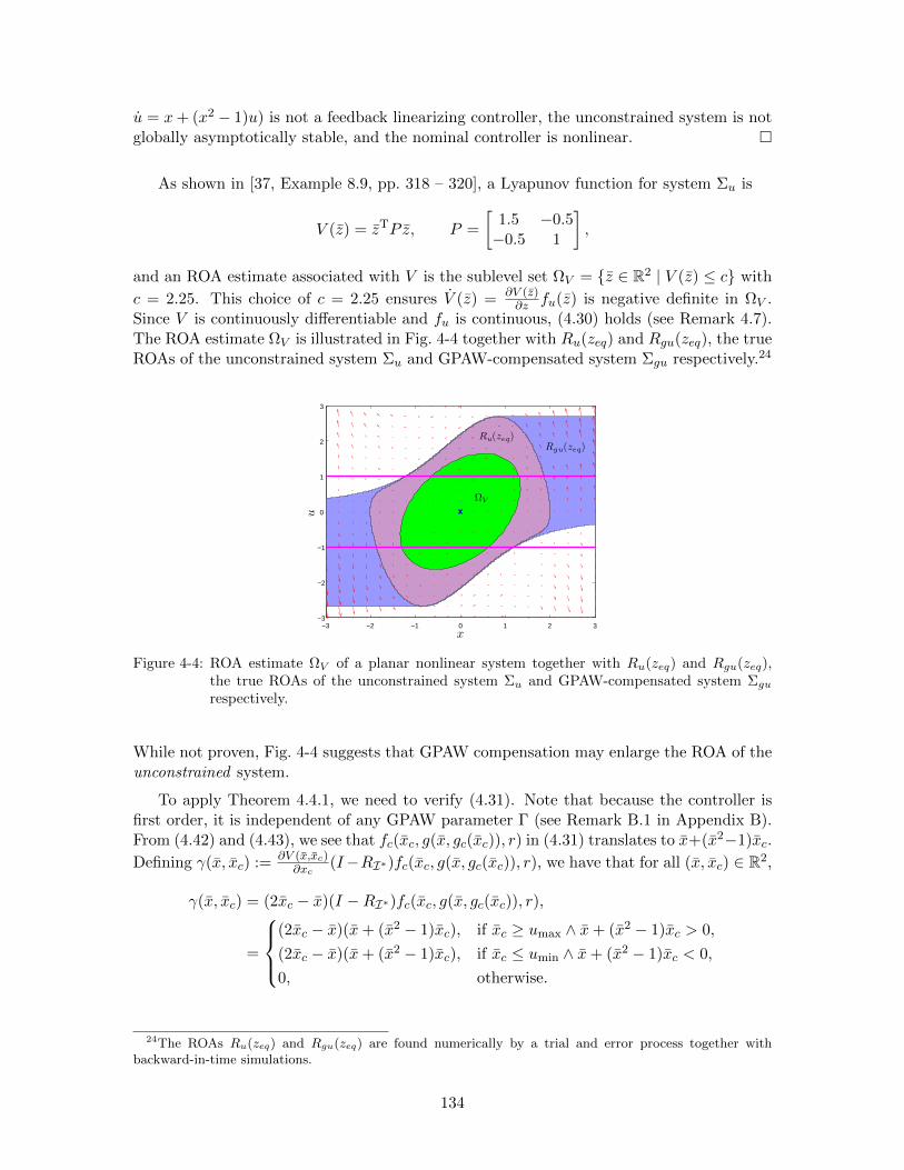
u = x+ (x2 − 1)u) is not a feedback linearizing controller, the unconstrained system is notglobally asymptotically stable, and the nominal controller is nonlinear.

As shown in [37, Example 8.9, pp. 318 – 320], a Lyapunov function for system Σu is

V (z) = zTP z, P =

[1.5 −0.5−0.5 1

],

and an ROA estimate associated with V is the sublevel set ΩV = z ∈ R2 | V (z) ≤ c with

c = 2.25. This choice of c = 2.25 ensures V (z) = ∂V (z)∂z fu(z) is negative definite in ΩV .

Since V is continuously differentiable and fu is continuous, (4.30) holds (see Remark 4.7).The ROA estimate ΩV is illustrated in Fig. 4-4 together with Ru(zeq) and Rgu(zeq), the trueROAs of the unconstrained system Σu and GPAW-compensated system Σgu respectively.24

−3 −2 −1 0 1 2 3−3

−2

−1

0

1

2

3

x

u

Ru(zeq)Rgu(zeq)

ΩV

Figure 4-4: ROA estimate ΩV of a planar nonlinear system together with Ru(zeq) and Rgu(zeq),the true ROAs of the unconstrained system Σu and GPAW-compensated system Σgu

respectively.

While not proven, Fig. 4-4 suggests that GPAW compensation may enlarge the ROA of theunconstrained system.

To apply Theorem 4.4.1, we need to verify (4.31). Note that because the controller isfirst order, it is independent of any GPAW parameter Γ (see Remark B.1 in Appendix B).From (4.42) and (4.43), we see that fc(xc, g(x, gc(xc)), r) in (4.31) translates to x+(x2−1)xc.

Defining γ(x, xc) := ∂V (x,xc)∂xc

(I−RI∗)fc(xc, g(x, gc(xc)), r), we have that for all (x, xc) ∈ R2,

γ(x, xc) = (2xc − x)(I −RI∗)fc(xc, g(x, gc(xc)), r),

=

(2xc − x)(x+ (x2 − 1)xc), if xc ≥ umax ∧ x+ (x2 − 1)xc > 0,

(2xc − x)(x+ (x2 − 1)xc), if xc ≤ umin ∧ x+ (x2 − 1)xc < 0,

0, otherwise.

24The ROAs Ru(zeq) and Rgu(zeq) are found numerically by a trial and error process together withbackward-in-time simulations.

134

For any (x, xc) ∈ R× ∂K = R× umin, umax, we have from the preceding,

γ(x, xc) =

(2umax − x)(x+ (x2 − 1)umax), if xc = umax ∧ x+ (x2 − 1)umax > 0,

(2umin − x)(x+ (x2 − 1)umin), if xc = umin ∧ x+ (x2 − 1)umin < 0,

0, otherwise.

By inspection of the preceding, we see that γ(x, xc) ≥ 0 for all (x, xc) = (x, umax) whenx ≤ 2umax = 2, and all (x, xc) = (x, umin) when x ≥ 2umin = −2. In other words, we have

γ(x, xc) ≥ 0, ∀(x, xc) ∈ ((−∞, 2]× umax) ∪ ([−2,∞)× umin) ⊂ R× ∂K. (4.44)

Condition (4.31) requires γ(x, xc) ≥ 0 for all (x, xc) ∈ ΩV ∩ (R × ∂K). Using thedefinition of ΩV (ΩV = z ∈ R2 | V (z) ≤ c for c = 2.25), it can be verified that

ΩV ∩ (R× ∂K) = (β+ × umax) ∪ (β− × umin),

where β+ :=[

13 −

√1718 ,

13 +

√1718

]= [−0.638, 1.305] and β− :=

[−1

3 −√

1718 ,−1

3 +√

1718

]=

[−1.305, 0.638]. Since β+ ⊂ (−∞, 2] and β− ⊂ [−2,∞), we see from (4.44) that γ(x, xc) ≥ 0for all (x, xc) ∈ (β+ × umax) ∪ (β− × umin) = ΩV ∩ (R× ∂K), which shows that (4.31)holds.

All hypotheses of Theorem 4.4.1 are satisfied, and we conclude from its application thatthe ROA of system Σgu contains ΩV ∩ (R ×K). Two sets of solutions, one starting fromz0 = (−1.2,−0.7) ∈ (ΩV ∩ (R × K)) ⊂ Ru(zeq) ⊂ Rgu(zeq) and another starting fromz0 = (2.8, 0) ∈ Rgu(zeq) \Ru(zeq) are shown in Fig. 4-5.

−3 −2 −1 0 1 2 3−3

−2

−1

0

1

2

3

x

u

φu(t, z0)

φgu(t, z0)

0 1 2 3 4 5 6 7 8 9 10−2

0

2

4

x

0 1 2 3 4 5 6 7 8 9 10−2

−1

0

1

2

u

time (s)

φu(t, z0)

φgu(t, z0)

Figure 4-5: Solutions of unconstrained and GPAW-compensated systems.

4.6 Chapter Summary

We showed that the GPAW-compensated controller, apart from being defined by the onlinesolution to a combinatorial optimization subproblem (see Section 2.5), can also be definedby the online solution to a convex quadratic program or a projection onto a convex polyhe-dral cone problem. Geometric properties of the projection operator were presented, leadingto a geometric bounding condition relating the vector fields of the nominal controller and

135

GPAW-compensated controller. The main results of this chapter are the ROA compari-son results Theorems 4.4.1, 4.4.2, and 4.4.3. Of note is Theorem 4.4.3, which yields anadmissible GPAW parameter when it is applicable. These ROA comparison results weredemonstrated on some simple (linear and nonlinear) planar systems. We note that attemptsto apply Theorems 4.4.1, 4.4.2, and 4.4.3 to some simple systems comprising open-loop un-stable plants have been unsuccessful. Whether or not Theorems 4.4.1, 4.4.2, and 4.4.3 areapplicable to systems with open-loop unstable plants requires further studies.

136

Chapter 5

Input Constrained MIMO LTISystems

In this chapter, we restrict consideration to regulatory GPAW-compensated systems com-prising input-constrained MIMO LTI plants driven by MIMO LTI controllers. In Section 5.1,we present the system descriptions which are simply specializations of the nonlinear case. Astability result (Theorem 5.2.1) specialized from Theorem 4.4.3 of Chapter 4 is presented inSection 5.2. Theorem 5.2.1 gives sufficient conditions to assert global asymptotic stabilityof the origin for the GPAW-compensated system. It is applicable only to systems withopen-loop stable plants, and is verified by solving a system of linear matrix inequalities,for which efficient solvers are readily available. While there are some attractive features,numerical experience suggest Theorem 5.2.1 to be a conservative result.

In Section 5.3, we study the familiar similarity transformation well known for LTI sys-tems, as applied to GPAW-compensated controllers. We show that the transformed GPAW-compensated controller derived from some nominal controller is equivalent to the GPAW-compensated controller derived from the transformed nominal controller, with the GPAWparameters related through the associated transformation matrix. Despite the GPAW-compensated controller being defined by the online solution to an optimization problem,similarity transformations can be easily performed.

In Section 5.4, we describe linear systems with partial state constraints, which has beenstudied in [103–106]. We present a way to transform the nominal controller into a canonicalform more convenient for GPAW compensation in Section 5.5. This canonical form isthen used in Section 5.6 to show that under a non-unique choice of the GPAW parameter,the GPAW-compensated system can be transformed into a linear system with partial stateconstraints. This allows results in existing literature (e.g. [103–106]) to be applied to thisclass of GPAW-compensated systems, and vice versa.

5.1 System Descriptions

Here, we describe the regulatory nominal system, unconstrained system, and GPAW-compensatedsystem when the unconstrained plant and nominal controller are both LTI. The input-constrained LTI plant corresponding to (1.1) is described by

x = Ax+B sat(u),

y = Cx+D sat(u),(5.1)

137

where x ∈ Rn is the state, u ∈ Rm is the control input, y ∈ Rp is the measurement,sat : Rm → Rm is the saturation function (1.2), and A ∈ Rn×n, B ∈ Rn×m, C ∈ Rp×n,D ∈ Rp×m are constant real matrices. We restrict consideration to regulatory systems, forwhich we assume r ≡ 0 in (2.26). Then the nominal LTI controller corresponding to (2.26)is described by1

xc = Acxc +Bcy,

uc = Ccxc,(5.2)

where xc ∈ Rq is the state, y ∈ Rp is the measurement, uc ∈ Rm is the controller output,and Ac ∈ Rq×q, Bc ∈ Rq×p, Cc ∈ Rm×q are constant real matrices. The nominal closed-loopsystem comprising (5.1) and (5.2) with u = uc can be written as

Σn :

x = Ax+B sat(Ccxc),

xc = BcCx+Acxc +BcD sat(Ccxc),or Σn : z = fn(z), (5.3)

where z := (x, xc) is the system state. Clearly, the unconstrained closed-loop system isdescribed by

Σu :

x = Ax+BCcxc,

xc = BcCx+ (Ac +BcDCc)xc,or Σu : z = fu(z) = Auz, (5.4)

with Au =[

A BCcBcC Ac+BcDCc

]∈ R(n+q)×(n+q).

Using the construction in Section 2.5, the GPAW-compensated controller correspondingto (2.27) and derived from the nominal controller (5.2) can be shown to be

xg = RI∗(xg, y)(Acxg +Bcy), xg(0)= xc(0),

ug = Ccxg,(5.5)

where xg ∈ Rq is the state, y ∈ Rp is the measurement, ug ∈ Rm is the controller out-put, (Ac, Bc, Cc) are defined by the nominal controller (5.2), and the projection operatorRI∗(xg, y) is to be defined next.2 Let the matrix Cc ∈ Rm×q in (5.2) and (5.5) be decom-posed into its rows as Cc = [c1, c2, . . . , cm]T, where ci ∈ Rq for all3 i ∈ Im. Following theconstruction in Section 2.5, define the 2m saturation constraint functions hi correspondingto (2.28) by

hi(xg) = cTi xg − umax,i, hi+m(xg) = −cT

i xg + umin,i, ∀i ∈ Im,

whose constant gradients are

∇hi = −∇hi+m = ci, ∀i ∈ Im.

For any index set I ⊂ I2m, define the q ×max|I|, 1 matrix corresponding to (2.29) by

NI =

[∇hσI(1),∇hσI(2), . . . ,∇hσI(|I|)], if I 6= ∅,0, otherwise,

1See Section 2.6 when the nominal LTI controller is of more general structure.2The construction of RI∗(xg, y) is presented in Section 2.5 and specialized for LTI systems here.3Recall that Ii := 1, 2, . . . , i for any positive integer i.

138

where σI : 1, 2, . . . , |I| → I is a chosen bijection described in Remark 2.5. For anyI ⊂ I2m such that rank(NI) = |I|, define the projection matrix corresponding to (2.30) by

RI =

I − ΓNI(N

TI ΓNI)

−1NTI , if I 6= ∅,

I, otherwise,(5.6)

where Γ = ΓT > 0 ∈ Rq×q is the GPAW parameter. Define the index set of active saturationconstraints and candidate solution set

Isat = i ∈ I2m | hi(xg) ≥ 0, J = I ⊂ Isat | |I| ≤ q.

Then at any fixed time (so that (xg(t), y(t)) are fixed), the projection operator RI∗(xg, y)in (5.5) is defined by (5.6) and a solution I∗ to the combinatorial optimization subproblemcorresponding to (2.31),

maxI∈J

F (I) = (Acxg +Bcy)TΓ−1RI(Acxg +Bcy),

subject to rank(NI) = |I|,NTIsatRI(Acxg +Bcy) ≤ 0.

(5.7)

Proposition 2.5.1 ensures that solutions I∗ to subproblem (5.7) always exist. See alsoTheorem 2.5.3 for the controller state-output consistency property, and Appendix C for aprocedure to apply GPAW compensation.

The GPAW-compensated closed-loop system comprising (5.1) and (5.5) with u = ugcan be written as

Σg :

x = Ax+B sat(Ccxg),

xg = RI∗(BcCx+Acxg +BcD sat(Ccxg)),or Σg : zg = fg(zg), (5.8)

where zg := (x, xg) and RI∗(Acxg +Bcy) := RI∗(xg, y)(Acxg +Bcy). When the state of theGPAW-compensated controller is initialized such that sat(xg(0)) = xg(0), Theorem 2.5.3(controller state-output consistency) yields sat(xg(t)) = xg(t) for all t ≥ 0. Then theGPAW-compensated system can be simplified to

Σgu :

x = Ax+BCcxg,

xg = RI∗(BcCx+ (Ac +BcDCc)xg),or Σgu : zg = fgu(zg), (5.9)

for all t ≥ 0, with the sat(·) function eliminated.4 As observed in Remark 2.19, the controllerstate can usually be initialized arbitrarily.

We assume the control objective is to regulate the system state about the origin zeq =(0, 0) ∈ Rn+q, which is clearly an equilibrium for systems Σn, Σu, Σg, and Σgu. To ensurethat zeq lies in the interior of the unsaturated region, assume also that the saturation limitsin (1.2) satisfy umin,i < 0 < umax,i for all i ∈ Im.

4This is discussed in Section 2.5 where (2.36) (analogous to Σgu (5.9)) is obtained.

139

5.2 A Stability Result for Systems with Open-loop StablePlants

Three region of attraction (ROA) comparison results were presented in Section 4.4. Ofnote is Theorem 4.4.3, which yields a prescribed GPAW parameter Γ = ΓT > 0 ∈ Rq×qsuch that GPAW compensation with parameter Γ ensures “global asymptotic stability” forthe equilibrium of the GPAW-compensated system Σg, in the sense that the ROA containsthe unsaturated region as in [103, 104]. In this section, we use Theorem 4.4.3 to derivea stability result for the GPAW-compensated system, for which the GPAW parameter isfound by solving a linear matrix inequality (LMI) problem [36, Section 2.2.1, p. 9]. Aswill be explained in Remark 5.1 below, this result applies only to systems with open-loopstable plants. A significant aspect is that the result depends only on properties of theunconstrained system Σu.

Theorem 5.2.1 (Global Asymptotic Stability for LTI GPAW-Compensated System). Con-sider the unconstrained system Σu (5.4). If there exist symmetric positive definite matricesP1 = PT

1 > 0 ∈ Rn×n and P2 = PT2 > 0 ∈ Rq×q such that[

P1 00 P2

] [A BCcBcC Ac +BcDCc

]+

[A BCcBcC Ac +BcDCc

]T [P1 00 P2

]< 0, (5.10)

then GPAW compensation with parameter Γ = P−12 yields systems Σg (5.8) and Σgu (5.9)

whose ROAs contain the unsaturated region Rn×K, where K = x ∈ Rq | sat(Ccx) = Ccx.

Proof. We will be applying Theorem 4.4.3 by comparing against the ROA of the uncon-

strained system Σu (see Remark 4.10). Define P :=[P1 00 P2

]and let V (z) := zTPz be a

Lyapunov function candidate for system Σu. Since P1 and P2 are symmetric positive def-inite, P is also symmetric positive definite, so that V is a positive definite function. It isalso clear that V is radially unbounded. Since Au =

[A BCcBcC Ac+BcDCc

]and (5.10) holds, we

have∂V (z)

∂zfu(z) = zT(PAu +AT

uP )z < 0, ∀z 6= 0. (5.11)

By [37, Theorem 4.2, p. 124], the origin zeq is a globally asymptotically stable equilibriumfor the unconstrained system Σu, so that the ROA of system Σu contains the unsaturatedregion Rn ×K. Since the vector fields fu (5.4) and fgu (5.9) coincide in the interior of theunsaturated region Rn× (K \ ∂K), it follows that zeq is also a locally asymptotically stableequilibrium for system Σgu.5

It can be verified that zeq satisfies (4.29), i.e. it is an equilibrium for the unconstrainedsystem Σu that lies within the interior of the unsaturated region. Moreover, since the outputequation of the nominal controller (5.2) is linear in the controller state, the unsaturatedregion K is convex (see Remark 4.4), so that K and Rn ×K are star domains with kernelsker(K) and Rn × ker(K) respectively (see Remark 4.2 and Corollary 4.2.2). It can beverified that zeq ∈ Rn × ker(K), and that V (z) = V (x, xc) has the form of (4.35) withVx(x) = xTP1x and Pc = P2. Moreover, since V is continuously differentiable and fu is

continuous, it follows that V (z) = ∂V (z)∂z fu(z) is continuous, and is also negative definite

5The vector fields fn and fg also coincide with fu in the interior of the unsaturated region, and zeq isalso a locally asymptotically stable equilibrium for systems Σn and Σg. However, these are not needed inthe proof.

140

due to (5.11). By [37, Lemma 4.3, p. 145], there exists a class K function α such that Vand fu satisfy (4.33).

All hypotheses of Theorem 4.4.3 are satisfied, and its application shows that GPAWcompensation with parameter Γ = P−1

c = P−12 yields system Σgu whose ROA contains the

unsaturated region Rn ×K. From the definitions of fg (5.8) and fgu (5.9), it can be seenthat fg and fgu coincide in the unsaturated region, which is a positively invariant set ofsystems Σg and Σgu due to Theorem 2.5.3. These imply that the ROAs of systems Σg andΣgu within the unsaturated region coincide, and yields the second conclusion, namely thatthe ROA of system Σg (with parameter Γ = P−1

2 ) also contains the unsaturated region.

Remark 5.1. When the matrix operations on the left-hand-side of (5.10) are carried out, itbecomes[

P1A+ATP1 P1BCc + CTBTc P2

(P1BCc + CTBTc P2)T P2(Ac +BcDCc) + (Ac +BcDCc)

TP2

]< 0. (5.12)

As implied by [124, Theorem 7.7.6, p. 472], necessary conditions for (5.12) (and (5.10)) tohold are that the diagonal blocks, i.e. P1A+ATP1 and P2(Ac+BcDCc)+(Ac+BcDCc)

TP2,must be negative definite. Hence it is necessary for A and Ac+BcDCc to be Hurwitz. Thisobservation actually follows from [182, Proposition 3.5]. This means that Theorem 5.2.1 canonly be applied to systems with stable open-loop plants. Moreover, if D = 0, Ac+BcDCc =Ac being Hurwitz means the nominal controller must also be stable.

The following example adapted from [182, Example 3.6] shows that A and Ac +BcDCcbeing Hurwitz is not sufficient to ensure the existence of P1 = PT

1 > 0 and P2 = PT2 > 0

satisfying (5.10).

Example 5.2.1. Let

Au =

[A BCcBcC Ac +BcDCc

]=

[−1 22 −1

].

It is clear that A = −1 and Ac + BcDCc = −1 are both Hurwitz. However, it can beverified that Au is not Hurwitz, with eigenvalues of −3 and +1. Hence no P1 = PT

1 > 0and P2 = PT

2 > 0 exist to satisfy (5.10). 4

Necessary and sufficient conditions to ensure existence of P1 = PT1 > 0 and P2 = PT

2 > 0that satisfy (5.10) are available in [182, Theorem 3.10] for a more general case. We note thatcondition (5.12) (and hence (5.10)) is an LMI, which admits efficient numerical solutions.This will be demonstrated in the next section on a simple example.

When the LMI (5.10) is feasible, Theorem 5.2.1 yields a GPAW parameter defined byΓ = P−1

2 . As discussed in Remark 2.25, it is desirable for Γ to have a small conditionnumber [124, p. 336]. In view of this, we formulate a generalized eigenvalue problem [36,Section 2.2.3, pp. 10 – 11] to minimize the condition number of the resultant GPAW param-eter, applicable whenever (5.10) is feasible. Since Γ = P−1

2 , the definition of its conditionnumber κ(Γ) [124, p. 336] yields

κ(Γ) = ‖Γ−1‖‖Γ‖ = ‖P2‖‖P−12 ‖ = κ(P2).

Hence minimizing κ(Γ) is equivalent to minimizing κ(P2). From [36, Section 3.2, p. 38], it

141

can be seen that the solution P2 = PT2 > 0 to the generalized eigenvalue problem

minP1,P2,µ,γ

γ,

subject to P1 > 0, µ > 0, µI < P2 < γµI,[P1A+ATP1 P1BCc + CTBT

c P2

(P1BCc + CTBTc P2)T P2(Ac +BcDCc) + (Ac +BcDCc)

TP2

]< 0,

(5.13)

is of minimal condition number, with P1, P2 satisfying (5.10). Application of Theorem 5.2.1remains unchanged, as will be shown in the next section.

5.2.1 Numerical Example

Here, we demonstrate an application of Theorem 5.2.1 on a simple system comprising a sat-urated second-order SISO LTI plant driven by a nominal second-order SISO LTI controller,where the objective is to regulate the system state about the origin.

The unconstrained stable plant is represented by the transfer function G(s) = 1s2+s+1

,which induces a saturated plant with state-space representation (5.1) where

A =

[0 1−1 −1

], B =

[01

], C =

[1 0

], D = 0.

Assume a nominal controller with transfer function K(s) = − 22.8s+11s2+8.6s+25

has been designedto improve the transient response of the system, that is to be interconnected with the plantby positive feedback. The nominal controller has a state-space representation (5.2) where

Ac =

[−8.6 −6.25

4 0

], Bc =

[40

], Cc =

[−5.7 −0.6875

].

The matrices (A, B, C, D, Ac, Bc, Cc) define the unconstrained system Σu (5.4) com-pletely, which is all the data required to apply Theorem 5.2.1. Using the LMI solver (orfunction) feasp of the MATLAB R© Robust Control Toolbox [183], symmetric positive defi-nite matrices P1f := P1 and P2f := P2 that satisfy the LMI (5.12) (and hence (5.10)) werefound to be

P1f =

[1.6090 0.317100.31710 0.66628

], P2f =

[1.3255 0.137300.13730 1.7704

].

Thus Theorem 5.2.1 shows that GPAW compensation with parameter

Γf = P−12f =

[0.76056 −0.058984−0.058984 0.56941

],

yields the GPAW-compensated systems Σg (5.8) and Σgu (5.9) whose ROAs contain theunsaturated region.

Using the solver (or function) gevp of the MATLAB R© Robust Control Toolbox [183],the solution to the generalized eigenvalue problem (5.13) was found to be

µ = 1.5046× 10−26, γ = 1.2012,

142

P1o =

[1.9132 0.392080.39208 0.78664

]× 10−26, P2o =

[1.5573 0.113540.11354 1.7544

]× 10−26.

Since we can always scale the GPAW parameter by a constant positive scalar (see Re-mark 2.15), we can use

Γo = 2.3948× 10−25P−12o =

[15.451 −1−1 13.715

],

as the normalized GPAW parameter. It can be verified that the condition numbers of Γf andΓo are κ(Γf ) = 1.4064 > κ(Γo) = 1.1997, which shows a marginal improvement (decrease)when solving the generalized eigenvalue problem (5.13) to obtain P1 and P2.

Remark 5.2. When the nominal controller (with transfer function K(s) = − 22.8s+11s2+8.6s+25

) isrepresented (equivalently) by matrices

Ac =

[0 1−25 −8.6

], Bc =

[01

], Cc =

[−11 −22.8

],

in (5.2), the numerical solutions change significantly. In particular, the condition numbersbecome κ(Γf ) = 22.324 and κ(Γo) = 17.441, representing a drastic deterioration. Thisshows that the numerical solutions are sensitive to coordinate transformations. Moreover,attempts to use nominal controllers with higher bandwidth, e.g. with K(s) = − 31s+17.4

s2+9.6s+30.6,

have failed in the sense that (5.10) and (5.13) becomes numerically infeasible. This suggeststhat Theorem 5.2.1 is a conservative result.

The GPAW-compensated controller (5.5) can be implemented in a few ways summa-rized in Appendix C. Here, we use the closed-form expressions (A.7) in Appendix A fora more efficient solution. The closed-form expressions (A.7) for the GPAW-compensatedcontroller (5.5) with parameter Γ are6

xg =

(I − ΓCT

c CcCcΓCT

c

)(Acxg +Bcy), if (ug ≥ umax) ∧ (Cc(Acxg +Bcy) > 0),(

I − ΓCTc Cc

CcΓCTc

)(Acxg +Bcy), if (ug ≤ umin) ∧ (Cc(Acxg +Bcy) < 0),

Acxg +Bcy, otherwise,

ug = Ccxg, xg(0) = xc(0).

For Γ = Γf and Γ = Γo, we have the matrices

I − ΓfCTc Cc

CcΓfCTc

=

[0.0015497 −0.12043−0.012848 0.99845

], I − ΓoC

Tc Cc

CcΓoCTc

=

[0.0051210 −0.12000−0.042458 0.99488

].

Two sets of solutions for the unconstrained system Σu (5.4), nominal system Σn (5.3),and GPAW-compensated system Σg (5.8) are shown in Fig. 5-1. The GPAW-compensatedsystems with parameters Γf and Γo are denoted by Σgf and Σgo respectively. In Fig. 5-1(a),the plant initial condition is x(0) = (1, 1), while in Fig. 5-1(b), the plant initial conditionis x(0) = (2, 2). In both cases, the controller states are set to zero and the plant stateis decomposed as x = [x1, x2]T. While Theorem 5.2.1 ensures global asymptotic stabilityfor the origin of Σgf and Σgo in the sense of [103], the time responses in Fig. 5-1 suggests

6Note that cc in (A.7) is given by cc = CTc . Moreover, ∧ denotes the logical AND operator.

143

0 0.5 1 1.5 2 2.5 3 3.5 4 4.5 5−1

0

1

2

x1

0 0.5 1 1.5 2 2.5 3 3.5 4 4.5 5−2

−1

0

1

x2

0 0.5 1 1.5 2 2.5 3 3.5 4 4.5 5

−2

−1

0

1

u

time (s)

Σu

Σn

Σgf

Σgo

(a) x(0) = (1, 1)

0 0.5 1 1.5 2 2.5 3 3.5 4 4.5 5−2

0

2

4

x1

0 0.5 1 1.5 2 2.5 3 3.5 4 4.5 5

−2

0

2

x2

0 0.5 1 1.5 2 2.5 3 3.5 4 4.5 5−5

0

5

u

time (s)

Σu

Σn

Σgf

Σgo

(b) x(0) = (2, 2)

Figure 5-1: Comparison of time responses of unconstrained system Σu, nominal system Σn, andGPAW-compensated systems Σgf (Γ = Γf ) and Σgo (Γ = Γo), all with zero initialconditions for the associated controllers.

there is little performance improvement when adopting the GPAW scheme. This can beattributed to the conservativeness of Theorem 5.2.1.

5.3 GPAW-Compensated Controller Transformations

Similarity transformations are fundamental operations for LTI systems. In this section,we establish the relation between the transformed GPAW-compensated controller and theGPAW-compensated controller derived from the transformed nominal controller.

For some nonsingular matrix T ∈ Rq×q, a similarity transformation is defined by xg =Txg, where xg is the state of the GPAW-compensated controller (5.5) derived from (5.2).The transformed GPAW-compensated controller with state xg is described by

˙xg = T xg = TRI∗(T−1xg, y)(AcT

−1xg +Bcy), xg(0) = Txc(0),

ug = CcT−1xg,

(5.14)

where xg = T−1xg. Define RI := TRIT−1 where RI is given by (5.6), written explicitly as

RI =

I − TΓNI(N

TI ΓNI)

−1NTI T−1, if I 6= ∅,

I, otherwise.(5.15)

Then the transformed GPAW-compensated controller (5.14) becomes

˙xg = RI∗(xg, y)(Acxg + Bcy), xg(0) = Txc(0),

ug = Ccxg,(5.16)

where I∗ is a solution to subproblem (5.7) with xg = T−1xg, and

Ac := TAcT−1, Bc := TBc, Cc := CcT

−1. (5.17)

144

Now, consider the transformation of the nominal controller (5.2) defined by the samematrix T and xc = Txc, where xc is the state of the nominal controller. The transformednominal controller with state xc is given by

˙xc = Acxc + Bcy, xc(0) = Txc(0),

uc = Ccxc,(5.18)

where Ac, Bc, Cc are defined in (5.17). In accordance with the construction in Section 2.5,applying GPAW compensation to the transformed nominal controller (5.18) with parameterΓ = ΓT > 0 ∈ Rq×q and state xg yields

˙xg = RI∗(xg, y)(Acxg + Bcy), xg(0) = Txc(0),

ug = Ccxg,(5.19)

where RI∗(xg, y) is to be defined. Observe that (5.19) differs from (5.16) only in theprojection operator RI∗(xg, y) and state definition xg. We will show that under a particularchoice of Γ, the two projection operators RI∗(xg, y) and RI∗(xg, y) are in fact equal, whichimplies the equivalence of the GPAW-compensated controllers (5.16) and (5.19).

Observe that the i-th row of Cc = CcT−1 is given by cT

i = cTi T−1, where ci is the i-th

row of Cc. Analogous to the saturation constraint functions hi, their gradients ∇hi, andthe matrices NI , RI in Section 5.1, we have

hi(xg) = cTi T−1xg − umax,i, hi+m(xg) = −cT

i T−1xg + umin,i,

∇hi = −∇hi+m = T−Tci,∀i ∈ Im, (5.20)

NI =

[∇hσI(1),∇hσI(2), . . . ,∇hσI(|I|)], if I 6= ∅,0, otherwise,

(5.21)

RI =

I − ΓNI(N

TI ΓNI)

−1NTI , if I 6= ∅,

I, otherwise.(5.22)

With the active saturation constraint set and candidate solution set

Isat = i ∈ I2m | hi(xg) ≥ 0, J = I ⊂ Isat | |I| ≤ q,

the projection operator RI∗(xg, y) in (5.19) is defined by (5.22) and a solution I∗ to thecombinatorial optimization subproblem analogous to (5.7)

maxI∈J

F (I) = (Acxg + Bcy)TΓ−1RI(Acxg + Bcy),

subject to rank(NI) = |I|,NTIsatRI(Acxg + Bcy) ≤ 0.

(5.23)

In relation to ∇hi and NI defined in Section 5.1, it can be seen that ∇hi = T−T∇hi andNI = T−TNI . Moreover, from (5.22) and (5.15), direct computation shows that RI = RI(= TRIT

−1) if and only if Γ = TΓTT. Therefore, when Γ = TΓTT, the transformed GPAW-compensated controller (5.16) is equivalent to the GPAW-compensated controller (5.19)derived from the transformed nominal controller (5.18), provided that subproblem (5.23)is equivalent to subproblem (5.7) when xg = Txg. Using (5.17), xg = Txg, Γ = TΓTT,

145

RI = TRIT−1, and NI = T−TNI , the objective function of subproblem (5.23) is

F (I) = (Acxg + Bcy)TΓ−1RI(Acxg + Bcy),

= (TAcT−1Txg + TBcy)T(TΓTT)−1TRIT

−1(TAcT−1Txg + TBcy),

= (Acxg +Bcy)TΓ−1RI(Acxg +Bcy) = F (I),

and the constraint functions are

rank(NI) = rank(T−TNI) = rank(NI),

NTIsatRI(Acxg + Bcy) = NT

IsatT−1TRIT

−1(TAcT−1Txg + TBcy) = NT

IsatRI(Acxg +Bcy),

which correspond to the objective and constraint functions of subproblem (5.7). Hencesubproblem (5.23) is equivalent to subproblem (5.7), which implies the equivalence of theGPAW-compensated controllers (5.16) and (5.19). We summarize this result in the follow-ing.

Proposition 5.3.1 (Similarity Transformation of GPAW-Compensated Controllers). LetT ∈ Rq×q be nonsingular, and consider the nominal controller (5.2), the GPAW-compensatedcontroller (5.5), and the transformed nominal controller (5.18) under the similarity trans-formation defined by xc = Txc. Under the similarity transformation defined by xg = Txg,the transformed GPAW-compensated controller (5.16) with parameter Γ is equivalent to theGPAW-compensated controller (5.19) with parameter TΓTT derived from the transformednominal controller (5.18).

With controllers (5.2), (5.18), (5.5), (5.16), and (5.19) denoted by Σcn, Σcn, Σcg, Σcg,and Σcg respectively, this result is illustrated in Fig. 5-2. Proposition 5.3.1 shows that given

Σcn Σcg

Σcn Σcg ≡ Σcg

GPAW, Γ

GPAW, TΓTT

T T

Figure 5-2: Illustration of transformation equivalence in Proposition 5.3.1 for some nonsingular ma-trix T ∈ Rq×q and symmetric positive definite Γ ∈ Rq×q.

some GPAW-compensated LTI controller (5.5) with parameter Γ, we can always transformit into an equivalent GPAW-compensated controller with parameter Γ = I, the identitymatrix. To see this, observe that Γ ∈ Rq×q is symmetric positive definite, so that it canalways be decomposed as Γ = ΦΦT for some nonsingular Φ ∈ Rq×q [124, Theorem 7.2.7,p. 406]. Using T = Φ−1 as the transformation matrix yields Γ = TΓTT = Φ−1ΦΦTΦ−T = I.Proposition 5.3.1 shows that the transformed GPAW-compensated controller (5.16) (withT = Φ−1) is equivalent to the GPAW-compensated controller (5.19) (with parameter Γ =TΓTT = I) derived from the transformed nominal controller (5.18) (with T = Φ−1). Sucha transformation may be convenient for realization purposes or further analysis.

146

5.4 Linear Systems with Partial State Constraints

Our next goal is to establish a link between GPAW-compensated LTI systems and linearsystems with partial state constraints, which has been studied in [103–106]. Such a link,like the relation with projected dynamical systems [107–110] (see Section 3.2), is strategic innature, and allows cross utilization of ideas and methods. Here, we describe linear systemswith partial state constraints.

Define the m-dimensional hypercube Dm ⊂ Rm by

Dm := (φ1, φ2, . . . , φm) ∈ Rm | −1 ≤ φi ≤ 1,∀i ∈ Im. (5.24)

Linear systems with partial state constraints are described by ODEs of the form [103]

θ = Agθ +Bgφ, θ(0) = θ0,

φ = h(Cgθ +Dgφ), φ(0) = φ0,(5.25)

where θ, θ0 ∈ Rnθ , φ, φ0 ∈ Dm are the (partial) states and initial states, and Ag, Bg, Cg, Dg

are real matrices of appropriate dimensions. Decomposing the vectors φ and Cgθ + Dgφinto φ = [φ1, φ2, . . . , φm]T and Cgθ+Dgφ = ψ = [ψ1, ψ2, . . . , ψm]T respectively, the functionh(Cgθ +Dgφ) = h(ψ) is defined by

h(Cgθ +Dgφ) = [h(ψ1, φ1), h(ψ2, φ2), . . . , h(ψm, φm)]T,

h(ψ, φ) =

0, if |φ| = 1, ψφ ≥ 0,

ψ, otherwise.

(5.26)

Existence and uniqueness of solutions to system (5.25) have been established in [103], to-gether with some sufficient conditions for the ROA of the origin to contain Rnθ × Dm.This ROA containment is called “global asymptotic stability” in [103, 104], which we haveadopted. See [104–106] for further results on linear systems with partial state constraints.

5.5 A Canonical Form for GPAW Compensation

Here, we transform the nominal controller (5.2) to an equivalent realization that is moreconvenient for GPAW compensation. This realization has the form

xcc = Accxcc +Bccy, xcc(0) = xcc0,

uc = Cccxcc =[0 Im

]xcc,

(5.27)

where Ij (for some positive integer j) is the j × j identity matrix, xcc, xcc0 ∈ Rq (q ≥ q)are the (possibly augmented) state and initial state, and the controller output uc is part ofthe controller state as implied by the special structure of Ccc =

[0 Im

](or Ccc = Im when

q = m). Since Cc ∈ Rm×q (see (5.2)), it is clear that rank(Cc) ≤ minm, q ≤ m [124, p. 13].Moreover, for any meaningful control design, Cc 6= 0 must hold, so that rank(Cc) > 0. Whenrank(Cc) = m, the transformation will yield q = q, i.e. the controller order is retained. Whenrank(Cc) < m the transformation will yield q > q, i.e. the transformed controller (5.27) is ofhigher order and must be a non-minimal realization of (5.2). As will be shown in Section 5.6,application of GPAW compensation on controllers of the form (5.27) with the particularform of Ccc yields a significant amount of simplification.

147

5.5.1 Full Row Rank Cc

Consider when rank(Cc) = m, which implies q ≥ m. Then all m rows of Cc are linearlyindependent. Defining q := q, we can choose a full rank matrix T ∈ R(q−m)×q such that

T :=[TCc

]∈ Rq×q is nonsingular (or define T := Cc if q = m). By defining xcc := Txc, it

can be verified that similarity transformation of (5.2) yields (5.27) with

Acc = TAcT−1, Bcc = TBc, Ccc = CcT

−1, xcc0 = Txc(0).

Since TT−1 =[TCc

]T−1 =

[T T−1

CcT−1

]= Iq =

[Iq−m 0

0 Im

], we see that CcT

−1 comprises the

lower m rows of the identity matrix Iq, so that we have Ccc = CcT−1 =

[0 Im

]as desired.

5.5.2 Row Rank Deficient Cc

Now, consider when α := rank(Cc) < m. Clearly, we have 0 < α < m, and there are αlinearly independent rows in Cc. We can choose a suitable permutation matrix P ∈ Rm×m,P−1 = PT [124, pp. 25 – 26] such that the topmost α rows of PCc are linearly independent.

Then the matrices P and PCc can be partitioned as PCc =[P1P2

]Cc =

[P1CcP2Cc

]=[Cc1Cc2

]where the rows of Cc1 := P1Cc ∈ Rα×q are linearly independent, and Cc2 := P2Cc ∈R(m−α)×q has all its rows linearly dependent on the rows of Cc1. For convenience, defineuc1 := Cc1xc, uc2 := Cc2xc and uc := (uc1, uc2), so that uc = PCcxc = Puc and uc = PTuc(due to P−1 = PT).

Since Cc1 ∈ Rα×q has full row rank (which implies q ≥ α), we can choose a full rank

matrix T ∈ R(q−α)×q such that T :=[TCc1

]∈ Rq×q is nonsingular (or define T := Cc1

if q = α). Defining xc := T xc, the transformed state equation of (5.2) and intermediateoutput uc1 are governed by

˙xc = TAcT−1xc + TBcy, xc(0) = T xc(0),

uc1 = Cc1T−1xc =

[0 Iα

]xc,

(5.28)

where Cc1T−1 =

[0 Iα

]follows from T T−1 =

[TCc1

]T−1 = Iq. Taking the time derivative

of uc2 and expressing in terms of xc yields

˙uc2 = Cc2AcT−1xc + Cc2Bcy, uc2(0) = Cc2xc(0). (5.29)

Based on (5.28) and (5.29), we can define an intermediate controller with augmentedstate xc := (xc, uc2) ∈ Rq, q = q +m− α, and output uc, described by

˙xc = Acxc + Bcy, xc(0) = xc0,

uc = PTuc = PT

[0 Iα 00 0 Im−α

]xc = PT

[0 Im

]xc,

(5.30)

where

Ac =

[TAcT

−1 0

Cc2AcT−1 0

], Bc =

[TCc2

]Bc, xc0 =

[TCc2

]xc(0).

Observe that uc = (uc1, uc2) forms the lower m elements of xc. It can be verified that theintermediate controller (5.30) can be obtained by similarity transformation of the q-th order

148

augmented nominal controller with state xca := (xc, uc2),

xca =

[Ac 0

Cc2Ac 0

]xca +

[IqCc2

]Bcy, xca(0) =

[IqCc2

]xc(0),

uc = PT

[Cc1 00 Im−α

]xca,

(5.31)

by defining xc := Tcaxca with Tca =[T 00 Im−α

].

Remark 5.3. Note that an equivalent realization of (5.31) is with the output equationuc =

[Cc 0

]xca. However, the form as presented in (5.31) is needed for effective use of

the augmented state uc2 in GPAW compensation, which manipulates the controller state toenforce the saturation constraints. The realization in (5.31) renders each output elementindependent of all other output elements, so that each can be saturated independently of allothers, allowing full exploitation of available control authority. See Section 5.5.3 for furtherdiscussions.

The output equation of (5.30) can be written as

uc = PT[0 Im

]xc =

[0 PT

]xc =

[0 Im

] [Iq−α 00 PT

]xc =

[0 Im

]T xc,

where T :=[Iq−α 0

0 PT

]∈ R(q+m−α)×(q+m−α) is nonsingular. The special structure of (5.27)

can then be obtained by a final similarity transformation defined by xcc := T xc = TTcaxca,which immediately yields Ccc =

[0 Im

]in (5.27). Partition the inverse matrix T−1 as

T−1 =[Ti1 Ti2

], and observe that

[TCc2

]=[

TPCc

]. The remaining vectors and matrices

in (5.27) are (see (5.30))

Acc = TAcT−1 = T

[TAcT

−1 0

Cc2AcT−1 0

] [Iq−α 0

0 P

],

= T

[TAcTi1 TAcTi2 0

Cc2AcTi1 Cc2AcTi2 0

]Iq−α 00 P1

0 P2

= T

[TAcTi1 TAcTi2P1,

Cc2AcTi1 Cc2AcTi2P1

],

= T

[TCc2

]Ac[Ti1 Ti2P1

]=

[Iq−α 0

0 PT

] [TPCc

]Ac[Ti1 Ti2P1

],

=

[TCc

]Ac[Ti1 Ti2P1

]=

[TCc

]AcT

−1

[Iq−α 0

0 P1

],

Bcc = TBc =

[Iq−α 0

0 PT

] [TCc2

]Bc =

[Iq−α 0

0 PT

] [TPCc

]Bc =

[TCc

]Bc,

xcc0 = T xc0 =

[Iq−α 0

0 PT

] [TCc2

]xc(0) =

[Iq−α 0

0 PT

] [TPCc

]xc(0) =

[TCc

]xc(0).

In the preceding expressions, recall that T ∈ R(q−α)×q is a full rank matrix chosen such thatT is nonsingular, and P1 is the top partition of the permutation matrix P .

149

5.5.3 Comments on Nominal Controller Transformations

Instead of the preceding techniques, the nominal controller (5.2) can always be transformedinto an equivalent non-minimal (q + m)-th order controller with state xcc := (xc, u), de-scribed by

xcc =

[Ac 0CcAc 0

]xcc +

[BcCcBc

]y, xcc(0) =

[IqCc

]xc(0),

u =[0 Im

]xcc,

which is of the form of (5.27). However, as stated in Remark 2.23, GPAW compensationwith Γ = Iq+m on this equivalent controller yields effectively no anti-windup compensation.Clearly, controller state augmentation for GPAW compensation needs further study, whichwe leave as future work (see Section 7.1.10).

On another aspect, observe that the GPAW scheme can be applied to the nominalcontroller (5.2) without any transformation to the form of (5.27). Doing so in the precedingsections is only to yield simplifications in the final controller description. When Cc is rowrank deficient, i.e. rank(Cc) = α < m, direct application of the GPAW scheme on (5.2)results in a closed-loop unsaturated region of the form Rn+q−α× Dα (or can be transformedto such a form), where Dα is a subset of the hypercube Dα in general (in fact Dα wouldbe a polyhedron with possibly more faces than the hypercube Dα). In other words, therecould be redundant saturation constraints. This means that the available control authoritymay not be exploited to the fullest, i.e. some control outputs that may not have reachedthe saturation limits may be inadvertently limited by other linearly dependent saturatedcontrol outputs. With the transformation in Section 5.5.2, the corresponding unsaturatedregion is of the form Rn+q−m×Dm = Rn+q−α×Dm, which is the type encountered in linearsystems with partial state constraints [103–106]. Doing so also allows each control outputto be constrained independently of other (originally linearly dependent) control outputs.We leave the study on effective handling of redundant saturation constraints as future work(see Section 7.1.10).

5.6 A Relation between GPAW-Compensated LTI Systemsand Linear Systems with Partial State Constraints

Here, we present a link between GPAW-compensated LTI systems and linear systems withpartial state constraints [103] described in Section 5.4. As mentioned in Section 5.4, thislink is strategic in nature and allows cross utilization of ideas and methods in GPAW com-pensation and existing literature. We show that under a (non-unique) choice of the GPAWparameter, the GPAW-compensated system (5.9) (or one obtained by GPAW compensationon a non-minimal equivalent realization of (5.2), e.g. the augmented controller (5.31)) canbe transformed into a linear system with partial state constraints of the form (5.25), whichhas been studied in [103–106]. Clearly, stability/performance properties of system (5.25)then carry over to system (5.9), and vice versa. This allows existing results in [103–106] tobe applied to such GPAW-compensated systems.

We start from the q-th order controller (5.27), which is a (possibly non-minimal) real-ization of the nominal controller (5.2). First, we need to make the assumption that the sat-

150

uration limits are symmetric,7 i.e. umax,i = −umin,i for all i ∈ Im (see (1.2)), and perform a

final similarity transformation of (5.27) by defining xc := Txcc, where T =[Iq−m 0

0 Λ

]∈ Rq×q

and Λ = diag(u−1max,1, u

−1max,2, . . . , u

−1max,m) ∈ Rm×m is the diagonal matrix with entries com-

prising the ordered reciprocals of the saturation limits. The transformed nominal controlleris then described by

˙xc = Acxc + Bcy, xc(0) = Txcc(0),

uc = Ccxc,(5.32)

whereAc = TAccT

−1, Bc = TBcc, Cc = CccT−1. (5.33)

The resulting q-th order GPAW-compensated controller is defined by the preceding matricesand has the form

˙xg = RI∗(xg, y)(Acxg + Bcy), xg(0) = Txcc(0),

ug = Ccxg.(5.34)

Application of GPAW compensation then proceeds as in Section 5.1, with some simplifica-tions to be described.

Due to the special structure of Ccc =[0 Im

](see (5.27)), it can be verified that each

row of Cc = CccT−1 =

[0 Λ−1

]= [c1, c2, . . . , cm]T has the form8

cTi = umax,i[~0

Tq−m, e

Ti ] = umax,i[~0

Tq−m, 0, . . . , 0︸ ︷︷ ︸

(i−1) zeros

, 1, 0, . . . , 0︸ ︷︷ ︸(m−i) zeros

] = umax,ieTq−m+i, ∀i ∈ Im,

where ~0q−m is the zero vector in Rq−m, ej ∈ Rm for j ∈ Im is the j-th standard basisvector in Rm with 1 as its j-th element and 0’s elsewhere, and ek ∈ Rq for k ∈ Iq isthe k-th standard basis vector in Rq. Partitioning the GPAW controller state in (5.34) asxg = (xgf , φ) ∈ Rq with xgf ∈ Rq−m and φ = [φ1, φ2, . . . , φm]T ∈ Rm as the partial states,the saturation constraint functions corresponding to (5.20) simplify to

hi(xg) = cTi xg − umax,i = umax,i[~0

Tq−m, e

Ti ]

[xgfφ

]− umax,i = umax,i(φi − 1),

hi+m(xg) = −cTi xg + umin,i = −umax,i[~0

Tq−m, e

Ti ]

[xgfφ

]− umax,i = −umax,i(φi + 1),

(5.35)

for all i ∈ Im. The corresponding constant gradient vectors are

∇hi = −∇hi+m = ci = umax,i[~0Tq−m, e

Ti ]T, ∀i ∈ Im.

Define the maps ς : I2m → Im and γ : I2m → −1,+1 by

ς(i) = ((i− 1) mod m) + 1, γ(j) =

+1, if j ∈ Im,−1, otherwise.

It can be seen that ς “wraps” any index in I2m to an index in Im, γ is a “sign” function in

7See also Section 3.6.8For clarity, we use the symbol ~0q−m to denote the (q−m) dimensional zero vector, only in this section.

151

some sense, and that ∇hi = γ(i)cς(i) for any i ∈ I2m. With these maps, for any I ⊂ I2m

such that |I| = s > 0, and any i ∈ Is, we have

∇hσI(i) = γ(σI(i))cς(σI(i)) = γ(σI(i))umax,ς(σI(i))[~0Tq−m, e

Tς(σI(i))]

T,

so that the matrix NI corresponding to (5.21) can be written as

NI =

[∇hσI(1),∇hσI(2), . . . ,∇hσI(s)] = ΩIΛI , if I 6= ∅,0, otherwise,

(5.36)

where9

ΩI =

[0(q−m)×s

eς(σI(1)) eς(σI(2)) . . . eς(σI(s))

]=∈ Rq×s,

ΛI = diag(γ(σI(1))umax,ς(σI(1)), . . . , γ(σI(s))umax,ς(σI(s))) ∈ Rs×s,

and 0(q−m)×s is the (q −m)× s zero matrix.

Remark 5.4. Observe that ΛI must be nonsingular because umax,i 6= 0 for all i ∈ Im.

For the GPAW parameter Γ, we choose it to be of the form Γ =[

Γ1 00 Im

], where Γ1 ∈

R(q−m)×(q−m) is symmetric positive definite. It can be verified that ΓΩI = ΩI holds for thischoice of Γ. Clearly the standard basis vectors satisfy eT

i ej = δij and eTi ej = δij , where δij

denotes the Kronecker delta function [125, p. 544]. Then when |I| = s > 0 and NI = ΩIΛIis full rank, it can be verified that ΩT

I ΓΩI = ΩTIΩI = Is, so that the projection matrix

corresponding to (5.22) can be written as

RI = Iq − ΓNI(NTI ΓNI)

−1NTI = Iq − ΓΩIΛI(Λ

TIΩTI ΓΩIΛI)

−1ΛTIΩTI ,

= Iq − ΩI(ΩTIΩI)

−1ΩTI = Iq − ΩIΩ

TI = Iq −

s∑i=1

eq−m+ς(σI(i))eTq−m+ς(σI(i)),

= Iq −∑j∈I

eq−m+ς(j)eTq−m+ς(j) = Iq −

∑j∈I

[0 00 eς(j)e

Tς(j)

]=

[Iq−m 0

0 II

], (5.37)

whereII = Im −

∑i∈I

eς(i)eTς(i). (5.38)

Notice that the definition of RI in (5.37) with (5.38) is also valid when I = ∅ since in thiscase, the summation in (5.38) will be over an empty set.

Next, we express the GPAW-compensated system (with the GPAW-compensated con-troller (5.34) derived from the transformed nominal controller (5.32)) in a form closer to thedescription of the linear system with partial state constraints (5.25). To do this, partition

the matrices Acc and Bcc in (5.27) appropriately as Acc =[Acc11 Acc12Acc21 Acc22

]and Bcc =

[Bcc1Bcc2

]respectively. Then, using the definition of T =

[Iq−m 0

0 Λ

], it can be verified that (see (5.33))

Ac =

[Acc11 Acc12Λ−1

ΛAcc21 ΛAcc22Λ−1

], Bc =

[Bcc1

ΛBcc2

], Cc =

[0 Λ−1

]. (5.39)

9For clarity, we use the symbol 0i×j to denote the i× j zero matrix, only in this section.

152

Using (5.37), the GPAW-compensated system (5.1), (5.34), with u = ug, is described by

x = Ax+B sat(Λ−1φ),

˙xgf = Bcc1Cx+Acc11xgf +Acc12Λ−1φ+Bcc1D sat(Λ−1φ),

φ = II∗(ΛBcc2Cx+ ΛAcc21xgf + ΛAcc22Λ−1φ+ ΛBcc2D sat(Λ−1φ)),

where II∗ in the last equation is defined by (5.38) and a solution I∗ to subproblem (5.23).By initializing the partial controller state φ in the unit hypercube, i.e. φ(0) ∈ Dm, we havesat(Λ−1φ(0)) = Λ−1φ(0). Then Theorem 2.5.3 yields sat(Λ−1φ(t)) = Λ−1φ(t) for all t ≥ 0,which implies φ(t) ∈ Dm and |φi(t)| ≤ 1 for all t ≥ 0 and all i ∈ Im (see (5.24)). Definingnθ := n+ q −m and θ := (x, xgf ) ∈ Rnθ , the preceding system can be written as

θ = Agθ +Bgφ, θ(0) = θ0,

φ = II∗(Cgθ +Dgφ), φ(0) = φ0,(5.40)

where θ0 = (x(0), T1xcc(0)) and φ0 = T2xcc(0) are the initial states, T1 =[Iq−m 0

]and

T2 =[0 Λ

]are the top and bottom partitions of the transformation matrix T =

[T1T2

], and

Ag =

[A 0

Bcc1C Acc11

], Bg =

[B

Acc12 +Bcc1D

]Λ−1,

Cg = Λ[Bcc2C Acc21

], Dg = Λ(Acc22 +Bcc2D)Λ−1.

It can be seen that system (5.40) has similarities with the linear system with partial stateconstraints (5.25). In fact, by comparing (5.40) with (5.25), we see that they are equivalentif and only if II∗(Cgθ +Dgφ) ≡ h(Cgθ +Dgφ) holds, or equivalently, if and only if

eTi II∗(Cgθ +Dgφ) = eT

i h(Cgθ +Dgφ), ∀i ∈ Im, ∀(θ, φ) ∈ Rnθ × Dm, (5.41)

holds, i.e. the individual elements are equivalent. We show this next.

Using the definition of II (see (5.38)), the left-hand-side of the equality in (5.41) is10

eTi II∗(Cgθ +Dgφ) = eT

i

(Im −

∑j∈I∗

eς(j)eTς(j)

)(Cgθ +Dgφ),

=(eTi −

∑j∈I∗

eTi eς(j)e

Tς(j)

)(Cgθ +Dgφ),

=

0, if (i ∈ I∗) ∨ ((i+m) ∈ I∗),eTi (Cgθ +Dgφ), otherwise,

(5.42)

where we have used eTi eς(j) = δiς(j) with δij being the Kronecker delta function [125, p. 544].

From the definitions of h and h in (5.26), the right-hand-side of the equality in (5.41) is

eTi h(Cgθ +Dgφ) = h(eT

i (Cgθ +Dgφ), φi),

=

0, if (|φi| = 1) ∧ (φie

Ti (Cgθ +Dgφ) ≥ 0),

eTi (Cgθ +Dgφ), otherwise.

(5.43)

10Note that ∨ denotes the logical OR operator.

153

To show that (5.41) holds, we need to show that (5.42) is equal to (5.43) for all i ∈ Im and all(θ, φ) ∈ Rnθ×Dm. Fix any (θ, φ) ∈ Rnθ×Dm. For any i ∈ Im such that eT

i (Cgθ+Dgφ) = 0,we see from (5.42) and (5.43) that the function values must be both zero regardless of theassociated logical conditions, and hence the equality in (5.41) holds. It remains to showthat the equality in (5.41) holds for all i ∈ Im such that eT

i (Cgθ + Dgφ) 6= 0. From (5.42)and (5.43), we see that the equality in (5.41) holds when11

((|φi| = 1) ∧ (φieTi (Cgθ +Dgφ) > 0))⇔ ((i ∈ I∗) ∨ ((i+m) ∈ I∗)). (5.44)

We will analyze subproblem (5.23) to show that (5.44) holds for all i ∈ Im. Since (θ, φ)is arbitrary, this implies that (5.41) holds, which in turn implies the equivalence of sys-tems (5.40) and (5.25).

First, partition the matrices Ag and Bg in (5.40) as Ag =[Ag1Ag2

]and Bg =

[Bg1Bg2

]where

Ag2 =[Bcc1C Acc11

]and Bg2 = (Acc12 + Bcc1D)Λ−1. Using (5.39), (5.1), xg = (xgf , φ),

and θ = (x, xgf ), it can be verified that

Acxg + Bcy =

[Acc11 Acc12Λ−1

ΛAcc21 ΛAcc22Λ−1

] [xgfφ

]+

[Bcc1

ΛBcc2

](Cx+DΛ−1φ),

=

[Bcc1Cx+Acc11xgf + (Acc12 +Bcc1D)Λ−1φ

ΛBcc2Cx+ ΛAcc21xgf + Λ(Acc22 +Bcc2D)Λ−1φ

],

=

[Ag2θ +Bg2φCgθ +Dgφ

]. (5.45)

Using (5.37), the objective function of subproblem (5.23) can be written as

F (I) = (Acxg + Bcy)TΓ−1RI(Acxg + Bcy) = (Acxg + Bcy)TΓ−1(Acxg + Bcy)− F1(I),

where

F1(I) =∑j∈I

(Acxg + Bcy)TΓ−1

[0 00 eς(j)e

Tς(j)

](Acxg + Bcy),

=∑j∈I

(Acxg + Bcy)T

[Γ−1

1 00 Im

] [0 00 eς(j)e

Tς(j)

](Acxg + Bcy),

=∑j∈I

(Acxg + Bcy)T

[0 00 eς(j)e

Tς(j)

](Acxg + Bcy) =

∑j∈I

∣∣∣[0 eTς(j)

](Acxg + Bcy)

∣∣∣2 ,=∑j∈I

∣∣∣∣[0 eTς(j)

] [Ag2θ +Bg2φCgθ +Dgφ

]∣∣∣∣2 =∑j∈I

∣∣eTς(j)(Cgθ +Dgφ)

∣∣2,and we have used

[0

eς(j)

][ 0 eT

ς(j) ] =[

0 00 eς(j)e

Tς(j)

]and (5.45). Since F1(I) is the only compo-

nent of F (I) that varies with I, it is clear that maximizing F (I) is equivalent to minimizingF1(I).

Next, we show that the rank condition of subproblem (5.23) always holds. Observefrom (5.35) that the constraints hi(xg) ≤ 0 and hi+m(xg) ≤ 0 cannot be simultaneously

11Observe that when φi 6= 0 and eTi (Cgθ + Dgφ) 6= 0, the condition φieTi (Cgθ + Dgφ) ≥ 0 implies

φieTi (Cgθ +Dgφ) > 0 holds with strict inequality.

154

active, i.e. (hi(xg) ≥ 0) ⇒ (hi+m(xg) < 0) and (hi+m(xg) ≥ 0) ⇒ (hi(xg) < 0). In otherwords, the constraints indexed by i ∈ Im and i+m ∈ (I2m \ Im) cannot be simultaneouslyactive. Hence for any I ⊂ Isat, I 6= ∅, the matrix ΩI ∈ Rq×|I| (see (5.36)) must becomposed of linearly independent standard basis vectors and hence full rank, i.e. rank(ΩI) =minq, |I| = |I|. Since ΛI is nonsingular for any I 6= ∅ (see Remark 5.4), we havefrom (5.36) that rank(NI) = rank(ΩIΛI) = rank(ΩI) = |I| [124, p. 13]. When I = ∅ ⊂ Isat,it is clear that rank(NI) = 0 = |I|, so that the rank condition of subproblem (5.23) alwaysholds.

When |Isat| = s > 0, the remaining constraint function of subproblem (5.23) reduces to

NTIsatRI(Acxg + Bcy) = ΛIsatΩ

TIsat

[Iq−m 0

0 II

] [Ag2θ +Bg2φCgθ +Dgφ

],

= ΛIsat

0s×(q−m)

eTς(σIsat (1))

...eTς(σIsat (s))

[Iq−m 00 II

] [Ag2θ +Bg2φCgθ +Dgφ

],

= ΛIsat

0s×(q−m)

eTς(σIsat (1))II

...eTς(σIsat (s))II

[Ag2θ +Bg2φCgθ +Dgφ

],

= ΛIsat [eς(σIsat (1)), . . . , eς(σIsat (s))]TII(Cgθ +Dgφ),

where we have used (5.36), (5.37), and (5.45). Then subproblem (5.23) is equivalent to12

minI∈J

F1(I) =∑j∈I

∣∣eTς(j)(Cgθ +Dgφ)

∣∣2,subject to ΛIsat [eς(σIsat (1)), . . . , eς(σIsat (s))]

TII(Cgθ +Dgφ) ≤ 0,

(5.46)

when |Isat| = s > 0. Observe from the objective function of subproblem (5.46) that F1(I) ≥0 for all I ⊂ Isat, F1(∅) = 0, and F1(I) will be minimized when I is of least cardinalitysuch that the associated constraints are satisfied (see also Proposition 2.5.2). Since forevery j ∈ Is, there is a unique i ∈ Isat such that σIsat(j) = i (see Remark 2.5), the j-thcomponent of the constraint function in subproblem (5.46) can be rewritten as

β(i, I) := eTj ΛIsat [eς(σIsat (1)), . . . , eς(σIsat (s))]

TII(Cgθ +Dgφ),

= γ(σIsat(j))umax,ς(σIsat (j))eTς(σIsat (j))II(Cgθ +Dgφ),

= γ(i)umax,ς(i)eTς(i)

(Im −

∑k∈I

eς(k)eTς(k)

)(Cgθ +Dgφ),

= γ(i)umax,ς(i)

(eTς(i) −

∑k∈I

eTς(i)eς(k)e

Tς(k)

)(Cgθ +Dgφ),

=

0, if ∃k ∈ I, ς(k) = ς(i),

γ(i)umax,ς(i)eTς(i)(Cgθ +Dgφ), otherwise,

(5.47)

where we have used the definition of II in (5.38) and ΛI in (5.36). Now, recall that

12We will not need the equivalent of subproblem (5.46) when |Isat| = 0, i.e. Isat = ∅.

155

constraints indexed by j ∈ Im and j + m ∈ (I2m \ Im) cannot be simultaneously active.Since I ⊂ Isat and i ∈ Isat, the condition (∃k ∈ I, ς(k) = ς(i)) in (5.47) can be verifiedto be equivalent to (∃k ∈ I, k = i), and hence equivalent to i ∈ I. Then the constraintβ(i, I) ≤ 0 holds when i ∈ I or γ(i)eT

ς(i)(Cgθ + Dgφ) ≤ 0. Since the constraint must hold

for the optimal solution I∗, i.e. β(i, I∗) ≤ 0 for all i ∈ Isat, we have

i ∈ I∗, or γ(i)eTς(i)(Cgθ +Dgφ) ≤ 0, ∀i ∈ Isat. (5.48)

Recall that we want to establish the equivalence (5.44) and we only need to consider thosei ∈ Im for which eT

i (Cgθ+Dgφ) 6= 0. First, assume that |φi| = 1 and φieTi (Cgθ+Dgφ) > 0

for some i ∈ Im. This corresponds to two cases:

(i) φi = 1 and φieTi (Cgθ +Dgφ) > 0; or

(ii) φi = −1 and φieTi (Cgθ +Dgφ) > 0.

In case (i), we have i ∈ Im ∩ Isat (see (5.35)) and

φieTi (Cgθ +Dgφ) = eT

i (Cgθ +Dgφ) = γ(i)eTς(i)(Cgθ +Dgφ) > 0.

Then i ∈ I∗ follows from (5.48). In case (ii), we have (i+m) ∈ (I2m \ Im) ∩ Isat and

φieTi (Cgθ +Dgφ) = −eT

i (Cgθ +Dgφ) = γ(i+m)eTς(i+m)(Cgθ +Dgφ) > 0.

Then i+m ∈ I∗ follows from (5.48). Together, these establish one direction of the equiva-lence (5.44), namely

((|φi| = 1) ∧ (φieTi (Cgθ +Dgφ) > 0))⇒ ((i ∈ I∗) ∨ ((i+m) ∈ I∗)).

It remains to show the converse.

We will show that if |φi| < 1 or φieTi (Cgθ + Dgφ) ≤ 0, then i, (i + m) 6∈ I∗. When

|φi| < 1, we have Isat = ∅, so that i, (i+m) 6∈ I∗ ⊂ Isat = ∅. Finally, consider when |φi| = 1and φie

Ti (Cgθ + Dgφ) ≤ 0. Then φie

Ti (Cgθ + Dgφ) < 0 holds with strict inequality due to

eTi (Cgθ +Dgφ) 6= 0. As before, this corresponds to two cases:

(iii) φi = 1 and φieTi (Cgθ +Dgφ) < 0; or

(iv) φi = −1 and φieTi (Cgθ +Dgφ) < 0.

In case (iii), we have i ∈ Im∩Isat and γ(i)eTς(i)(Cgθ+Dgφ) < 0, which implies (i+m) 6∈ Isat,

(i+m) 6∈ I∗ ⊂ Isat, and eTς(i)(Cgθ +Dgφ) 6= 0. From (5.47), it can be seen that β(i, I) ≤ 0

for any I ⊂ Isat. Due to eTς(i)(Cgθ + Dgφ) 6= 0, we must have i 6∈ I∗ to minimize the

objective function of subproblem (5.46), and hence i, (i + m) 6∈ I∗. Finally, in case (iv),we have (i + m) ∈ (I2m \ Im) ∩ Isat and γ(i + m)eT

ς(i+m)(Cgθ + Dgφ) < 0, which implies

i 6∈ Isat, i 6∈ I∗ ⊂ Isat, and eTς(i+m)(Cgθ + Dgφ) 6= 0. The same argument then shows that

(i + m) 6∈ I∗ and hence i, (i + m) 6∈ I∗. These establish the equivalence (5.44) and showthat the GPAW-compensated system (5.40) is indeed equivalent to the linear system withpartial state constraint (5.25).

System (5.40) is obtained by GPAW compensation with parameter Γ on the transformednominal controller (5.32). Using Proposition 5.3.1, we can recover the GPAW parameter inthe original coordinates as Γ = T−1ΓT−T = (TTΓ−1T )−1. We summarize this result whenCc has full row rank below, which uses relations in (5.32) and Section 5.5.1.

156

Theorem 5.6.1 (GPAW-Compensated LTI System as Linear System with Partial StateConstraints). If Cc in (5.2) satisfies rank(Cc) = m, then GPAW compensation applied tothe nominal controller (5.2) yields a closed-loop system (5.9) that can be transformed toa linear system with partial state constraints (5.25) when the GPAW parameter Γ has theform

Γ = T−1ΓT−T = (TTΓ−11 T + CT

c Λ2Cc)−1,

where

T =

[T

ΛCc

]∈ Rq×q, Γ =

[Γ1 00 Im

]∈ Rq×q,

Λ = diag(u−1max,1, u

−1max,2, . . . , u

−1max,m) ∈ Rm×m,

T ∈ R(q−m)×q is chosen such that T is nonsingular, and Γ1 ∈ R(q−m)×(q−m) is symmetricpositive definite. Moreover, the transformation is defined by xg = Txg, where xg and xg arethe states of the transformed and original GPAW-compensated controllers respectively.

Remark 5.5. When Cc is row rank deficient, an analogous form of Theorem 5.6.1 where theGPAW-compensated controller is derived from the augmented nominal controller (5.31) canbe stated, but is omitted for brevity.

For this class of GPAW-compensated systems, it may be more efficient to implementthe associated GPAW-compensated controller as the transformed linear system with partialstate constraints (5.25), since these are closed-form expressions and no optimization problemneeds to be solved online (see also Section B.1 in Appendix B).

5.6.1 Illustration of an Existing Result

With Theorem 5.6.1, results from [103–106] can be applied to this class of GPAW-compensatedsystems. As an illustration, we state the following which is a direct translation of a stabilityresult in [103].

Theorem 5.6.2 (Hou et al. [103, Theorem 3]). Consider the transformed GPAW-compensated

system (5.40). If the matrix[Ag BgCg Dg

]is Hurwitz stable and there exist symmetric positive

definite matrices P1 ∈ Rnθ×nθ , P2 ∈ Rm×m, and Q ∈ R(nθ+m)×(nθ+m) such that P2 = [pij ]satisfies

pii ≥m∑

j=1,j 6=i|pji|, ∀i ∈ Im,

and [P1 00 P2

] [Ag BgCg Dg

]+

[Ag BgCg Dg

]T [P1 00 P2

]= −Q,

then the region of attraction of the origin of system (5.40) contains Rnθ×Dm, i.e. the originis globally asymptotically stable in the sense of [103].

Proof. See [103].

Under the similarity transformation defined by xg = Txg for some nonsingular T ∈ Rq×q,the corresponding unsaturated region in the original coordinates is X := Rn×T−1(Rq−m×Dm). Hence in the original coordinates, the region of attraction of the origin for the GPAW-compensated system (5.9) must contain X. See [104–106] for other applicable results.

157

5.7 Chapter Summary

In this chapter, we restrict consideration to regulatory GPAW-compensated systems com-prising input-constrained MIMO LTI plants driven by MIMO LTI controllers. A stabilityresult that is specialized from the nonlinear case was presented, which is readily verified bysolving a system of linear matrix inequalities. Even though global asymptotic stability isassured, numerical experience suggests this result to be conservative.

Similarity transformations are fundamental operations for LTI systems. Even though theGPAW-compensated controller is defined by the online solution to an optimization problem,similarity transformations can still be performed without much difficulty. We showed howto transform the nominal LTI controller into a canonical form that is more convenient forGPAW compensation. This canonical form is then used to show that under some non-uniquechoice of the GPAW parameter, the GPAW-compensated system can be transformed intoa linear system with partial state constraints, a topic that has been previously studied.This allows results in existing literature to be applied to this class of GPAW-compensatedsystems, and vice versa.

158

Chapter 6

Numerical Comparisons

In this chapter, we compare the GPAW scheme against the nonlinear anti-windup scheme forEuler-Lagrange systems proposed in [24], the anti-windup scheme for feedback linearizablenonlinear systems proposed in [65], and the LMI-based anti-windup scheme for stable LTIsystems proposed in [128]. As our stability results obtained thus far are somewhat conser-vative, we will not establish analytical stability of the GPAW-compensated systems. Thesenumerical comparisons only show that GPAW compensation can yield numerically compa-rable performance for the cases studied. Note also that the stability results of [24, 65, 128]are of the “absolute” sense, the drawback of which was discussed in Section 3.7.

6.1 Nonlinear Anti-windup Scheme

The nonlinear anti-windup scheme of [24] was briefly described in Section 1.4.4. As men-tioned, the method was first proposed in [74] and extended to Euler-Lagrange systemsin [24], where two simulation studies were presented. Here, we compare the GPAW schemeagainst the nonlinear anti-windup scheme using one of the two simulation studies, whichis on a double integrator plant driven by a PID controller. The main aspect to note fromthis study is the effect of controller state initialization (see the statement of Problem 1 inSection 1.3).

Remark 6.1. Attempts have been made to compare the GPAW scheme against the nonlinearanti-windup scheme using the four-link robot example in [24]. One difficulty is that theexpressions for the generalized inertia matrix and Coriolis forces/torques were not provided.Clarifications with Prof. Luca Zaccarian, co-author of [24], indicates that the expressionsare available in [184, pp. 105 – 106]. However, even using these expressions, we have beenunable to reproduce the results in [24] for the robot example.

The double integrator plant is described by

x = Ax+B sat(u), x(0)= x0,

y = x,A =

[0 10 0

], B =

[01

], (6.1)

where x is the state, y = [y1, y2]T is the measurement, u is the control, and the saturationfunction (1.2) is defined by umax = −umin = 0.25. The nominal PID controller is

ei = r − y1, ei(0) = ei0,

uc = kp(r − y1) + kiei − kdy2,(6.2)

159

where (kp, ki, kd) = (8, 4, 4). Here, the reference input r is a constant so that r ≡ 0.The closed-loop system comprising (6.1) and (6.2) with u = uc is the nominal system anddenoted by Σn. When the plant is unconstrained, i.e. umax = −umin = ∞, the sameclosed-loop system (6.1), (6.2) will be called the unconstrained system and denoted by Σu.

6.1.1 Nonlinear Anti-windup Compensated System

The nonlinear anti-windup compensator1 is described by [24]

xe = Axe +B(sat(sat(uc) + v1)− uc), xe(0) = xe0,

v1 = −Kg sat(K−1g Kqxe1)− γE(xe1, xe2)K0xe2,

γE(xe1, xe2) =

1, if xe1xe2 ≥ 0,Kg sat(K−1

g Kqxe1)Kqxe1

, otherwise,

(6.3)

where xe = [xe1, xe2]T is the state and (Kg,Kq,K0) = (0.99, 80, 100) are the anti-windupgains. To incorporate the anti-windup compensator (6.3), the nominal controller (6.2) ismodified by replacing measurement y with y − xe, i.e.

ei = r − (y1 − xe1), ei(0) = ei0,

uc = kp(r − (y1 − xe1)) + kiei − kd(y2 − xe2),(6.4)

while the final anti-windup compensated controller output becomes2

u = sat(uc) + v1. (6.5)

The nonlinear anti-windup compensated controller induced by the nonlinear anti-windupcompensator (6.3) is then defined by (6.3), (6.4), and (6.5). The closed-loop system (6.1),(6.3), (6.4), and (6.5), will be called the nonlinear anti-windup compensated system anddenoted by Σaw.

6.1.2 Approximate Nominal System

It can be seen from the description of the nominal controller (6.2) that the output equationis dependent on measurements and reference input, hence is of the form (2.24). We use thetechnique of Section 2.6 (see also Section 2.8.1 and Section A.2 in Appendix A) to obtainan approximate nominal controller of the form (2.26) described by

xc1 = r − y1, xc1(0) = ei0,

xc2 = a(kp(r − y1)− kdy2 − xc2), xc2(0) = kp(r − y1(0))− kdy2(0),

uc = kixc1 + xc2,

1See Sections 1.2 and 1.3.1 for discussions on the distinction between an anti-windup compensator andthe associated anti-windup compensated controller.

2In [24], the control signal u is defined with an additional saturation, i.e. u = sat(sat(uc) + v1). Becausethe input to the plant (6.1) is already constrained, this final saturation is redundant. If the convention of [24]is adopted, the control signal will be artificially constrained and may give the false appearance of achievingcontroller state-output consistency (see Theorem 2.5.3).

160

where a > 0 is the approximation parameter. Notice that the augmented state xc2 canapproximate the signal kp(r − y1) − kdy2 arbitrarily well when a > 0 is chosen sufficientlylarge. The preceding approximate nominal controller can be written as

xc = Acxc +Bcyy +Bcrr, xc(0) = xc0,

uc = Ccxc,(6.6)

Ac =

[0 00 −a

], Bcy =

[−1 0−akp −akd

], Bcr =

[1akp

], Cc =

[ki 1

],

where xc0 = [ei0, kp(r − y1(0))− kdy2(0)]T.

The closed-loop system comprising (6.1) and (6.6) with u = uc will be called the nominalapproximate system and denoted by Σna. When umax = −umin =∞, the same closed-loopsystem (6.1) and (6.6) will be called the unconstrained approximate system and denoted byΣua. System Σua can written as

xua = Auaxua +Buar, Aua =

[A BCcBcy Ac

], Bua =

[0Bcr

],

where xua := (x, xc). Clearly, for the nominal approximate system Σna to be at leastlocally stable, it is necessary for Aua to be Hurwitz. By applying the Routh Criterion [185,p. 177] to the characteristic polynomial of Aua, it can be shown that Aua is Hurwitz whena > 2.6559 for (kp, ki, kd) = (8, 4, 4). By comparing the time responses for different valuesof a as in Section 2.8.1, it was found that setting a = 50 gives a good approximation ofsystems Σna, Σua to systems Σn, Σu respectively. Hence we fix a = 50.

6.1.3 GPAW-Compensated System

Applying GPAW compensation to the approximate nominal controller (6.6) yields theGPAW-compensated controller (2.27), which, using the closed-form expressions (A.7) inAppendix A, can be written as

xg =

(I − 1

CcΓCTc

ΓCTc Cc

)(Acxg +Bcyy +Bcrr), if Amax ∨Amin,

Acxg +Bcyy +Bcrr, otherwise,

ug = Ccxg, xg(0) = xg0,

(6.7)

Amax = (ug ≥ umax) ∧(Cc(Acxg +Bcyy +Bcrr) > 0

),

Amin = (ug ≤ umin) ∧(Cc(Acxg +Bcyy +Bcrr) < 0

).

We fix the GPAW parameter as the identity matrix Γ = I. The closed-loop system com-prising (6.1) and (6.7) with u = ug and xg0 = xc0 will be called the GPAW-compensatedsystem and denoted by Σg.

For reasons that will become obvious in the next section, we note that the controllerstate can be arbitrarily initialized. To improve the transient response, we will initialize itwithin the unsaturated region, i.e. xg0 ∈ K := x ∈ R2 | sat(x) = x. Decompose thecontroller state and initial state as xg = [xg1, xg2]T and xg0 = [xg01, xg02]T respectively. Forxg2 to be a good approximation of the signal kp(r− y1)− kdy2 starting from time t = 0, we

161

need xg2(0) = xg02 = kp(r − y1(0))− kdy2(0). Then it can be verified that setting3

xg1(0) = xg01 =sat(Ccxc0)− xg02

ki,

where xc0 is the initial controller state for the approximate nominal controller (6.6), ensuresxg(0) = xg0 ∈ K. As will be seen in the next section, this initialization yields significantimprovements in the transient response. We denote the GPAW-compensated system withthe described controller state initialization by Σgi.

6.1.4 Numerical Results

The unconstrained system Σu, nominal system Σn, nonlinear anti-windup compensatedsystem Σaw, and GPAW-compensated systems Σg, Σgi, are simulated for r being a unitstep input. The time responses are shown in Fig. 6-1. Observe that system Σg exhibits

0 1 2 3 4 5 6 70

0.5

1

1.5

x1

0 1 2 3 4 5 6 7−0.5

0

0.5

u

time (s)

Σu

Σn

Σaw

Σg

Σgi

0 2 4 6 8 10 12 14 16 18 20−6

−4

−2

0

2

4

x1

0 2 4 6 8 10 12 14 16 18 20−50

0

50

100

150

200

u

time (s)

Σu

Σn

Σaw

Σg

Σgi

Figure 6-1: Time responses for double integrator plant. The left plot shows a close-up view, whilethe right plot shows a macro view. Observe that system Σg exhibits a stable responsedespite having a sluggish transient. The controller state initialization for system Σgi

improves the transient response significantly.

a stable response with a sluggish transient. The controller state initialization xg0 ∈ Kimproves the transient response of system Σgi significantly.

Now, compare the responses of systems Σaw and Σgi. Observe that the GPAW-compensatedsystem Σgi expends significantly less control effort in comparison to the nonlinear anti-windup compensated system Σaw. Moreover, controller state-output consistency (Theo-rem 2.5.3) holds for the GPAW-compensated systems Σg and Σgi, but does not apply tothe nonlinear anti-windup compensated system Σaw. In terms of the output response x1, Σgi

has an initially faster response but reaches steady state later. We see that the performanceof system Σgi is comparable to that of system Σaw.

6.2 Two Anti-windup Schemes for Nonlinear Systems

In this section, we compare the GPAW scheme against two anti-windup schemes developedfor nonlinear systems, using the example in [65]. The first is proposed in [65] and applicable

3Note that this is similar to back-calculation [53], but applied only to controller state initialization.

162

to feedback linearizable nonlinear systems. This method has the attractive feature that theanti-windup compensator is fully defined independent of any parameters. The second is thenonlinear anti-windup scheme for Euler-Lagrange systems [24] that was also compared inSection 6.1.

The second order saturated feedback linearizable nonlinear plant is described by [65]

x =

[x2

−10x1−0.1x31−48.54x2−w+sat(u)6.67(1+0.1 sinx1)

],

y = x,

(6.8)

where x = [x1, x2]T ∈ R2 is the state, u ∈ R is the control input, w ∈ R is a disturbanceinput, and y ∈ R2 is the measurement. The saturation limits are umax = −umin = 100 [65].A feedback linearizing controller was designed in [65] and described by

xc = x1 − r,uc = 10x1 + 0.1x3

1 + 48.54x2

+ 6.67(1 + 0.1 sinx1)(−kp(x1 − r)− 200(x2 − ˙r)− 6400xc − ¨r),

(6.9)

where kp > 0 is the proportional gain, xc ∈ R is the controller state, y = x = [x1, x2]T isthe measurement, r := [r, ˙r, ¨r]T is the reference input, and uc ∈ R is the controller output.

Remark 6.2. We will show in Section 6.2.5 that the nominal design in [65] with kp = 400corresponds to a design with poorly damped dynamics for the unconstrained system. Aswill be shown, more reasonable designs with good damping can be obtained by simplyincreasing kp.

The closed-loop system comprising (6.8) and (6.9) with u = uc will be called the nominalsystem and denoted by Σn. The same closed-loop system with the plant unconstrained,i.e. umax = −umin =∞, will be called the unconstrained system and denoted by Σu. It canbe verified that the unconstrained system can be written as

xcl = Aclxcl +

0

− w6.67(1+0.1 sinx1) + kpr + 200 ˙r − ¨r

−r

,Acl =

0 1 0−kp −200 −6400

1 0 0

, (6.10)

where xcl := [x1, x2, xc]T is the state of the closed-loop system.

6.2.1 Feedback Linearized Anti-windup Compensated System

For distinction and ease of reference, we will call the anti-windup scheme of [65] the feedbacklinearized anti-windup scheme.4 As shown in [65], the associated anti-windup compensator5

4This is just a name for ease of distinguishing between the different anti-windup schemes introduced. Itdoes not imply that the anti-windup compensator uses feedback linearization in any significant way.

5See Sections 1.2 and 1.3.1 for discussions on the distinction between an anti-windup compensator andthe associated anti-windup compensated controller.

163

is given by

xaw =

[0 1−kp −200

]xaw +

[01

]uc − sat(uc)

6.67(1 + 0.1 sinx1),

ξ = −[1 0

]xaw,

(6.11)

where ξ ∈ R is the anti-windup compensator output. To incorporate the preceding anti-windup compensator, the state equation of the nominal controller (6.9) is modified with ξ,resulting in the modified nominal controller

xc = x1 − r − ξ,uc = 10x1 + 0.1x3

1 + 48.54x2

+ 6.67(1 + 0.1 sinx1)(−kp(x1 − r)− 200(x2 − ˙r)− 6400xc − ¨r).

(6.12)

The closed-loop system comprising (6.8), (6.11), and (6.12), with u = uc, will be calledthe feedback linearized anti-windup compensated system and denoted by Σawf .

6.2.2 Nonlinear Anti-windup Compensated System

The nonlinear anti-windup compensator for the plant (6.8) can be verified to be [24]

xe =

[xe2

f(x, xe, u, uc)

],

v1 = γ(x, x− xe),(6.13)

where xe = [xe1, xe2]T is the state, v1 ∈ R is the anti-windup compensator output, and

f(x, xe, u, uc) =−10x1 − 0.1x3

1 − 48.54x2 + sat(u)

6.67(1 + 0.1 sinx1)

− −10(x1 − xe1)− 0.1(x1 − xe1)3 − 48.54(x2 − xe2) + uc6.67(1 + 0.1 sin(x1 − xe1))

,

γ(x, x− xe) = 10x1 + 0.1x31 − 10(x1 − xe1)− 0.1(x1 − xe1)3

−Kg sat(K−1g Kqxe1)− γE(xe1, xe2)K0xe2,

= 10xe1 + 0.1(x31 − (x1 − xe1)3)−Kg sat(K−1

g Kqxe1)− γE(xe1, xe2)K0xe2,

γE(xe1, xe2) =

1, if xe1xe2 ≥ 0,Kg sat(K−1

g Kqxe1)Kqxe1

, otherwise.

The output of the anti-windup compensated controller is given by6

u = sat(uc) + v1. (6.14)

In [65], the anti-windup gains were chosen to be (Kg,Kq,K0) = (0.99, 240, 100).

To incorporate the nonlinear anti-windup compensator (6.13), the measurement input

6In [24], the controller output u is with an extra saturation, i.e. u = sat(sat(uc)+v1). This final saturationhas been incorporated in the plant (6.8) and hence redundant.

164

of the nominal controller (6.9) is modified from y to y − xe to yield

xc = x1 − xe1 − r,uc = 10(x1 − xe1) + 0.1(x1 − xe1)3 + 48.54(x2 − xe2) + 6.67(1 + 0.1 sin(x1 − xe1))

× (−kp(x1 − xe1 − r)− 200(x2 − xe2 − ˙r)− 6400xc − ¨r).

(6.15)

The closed-loop system comprising (6.8), (6.13), (6.15), and (6.14), will be called thenonlinear anti-windup compensated system and denoted by Σawn.

6.2.3 Approximate Nominal System

It can be seen from the description of the nominal controller (6.9) that the output equationis dependent on measurements and reference input, hence is of the form (2.24). We use thetechnique of Section 2.6 (see also Section 2.8.1) to obtain an approximate nominal controllerof the form (2.26) described by

xc1 = x1 − r,xc2 = a(z1(y)− xc2),

xc3 = a(z2(y, r)− xc3),

uc = xc1xc2 + xc3,

(6.16)

where a > 0 is the approximation parameter and

z1(y) := −6400× 6.67(1 + 0.1 sinx1),

z2(y, r) := 10x1 + 0.1x31 + 48.54x2 + 6.67(1 + 0.1 sinx1)(−kp(x1 − r)− 200(x2 − ˙r)− ¨r).

Notice that the augmented state variables (xc2, xc3) can approximate (z1(y), z2(y, r)) arbi-trarily well when a > 0 is chosen sufficiently large. To ensure good approximation of thesesignals from t = 0 onwards, we initialize these augmented states according to

xc2(0) = z1(y(0)), xc3(0) = z2(y(0), r(0)). (6.17)

Given the initial state xc0 of the nominal controller (6.9), the remaining state is initializedas xc1(0) = xc0.

The closed-loop system comprising (6.8) and (6.16) with u = uc will be called thenominal approximate system and denoted by Σna. When umax = −umin = ∞, the sameclosed-loop system (6.8), (6.16) will be called the unconstrained approximate system anddenoted by Σua. By comparing the time responses for different values of a > 0 as inSection 2.8.1, it was found that setting a = 200 gives a good approximation of systems Σna,Σua to systems Σn, Σu respectively. The responses of these systems to the reference anddisturbance input w = w1 defined in (6.18) are shown in Fig. 6-2. We fix the approximationparameter as a = 200.

6.2.4 GPAW-Compensated System

The approximate nominal controller (6.16) can be written in the form (2.26), which definesthe functions fc and gc. Applying GPAW compensation to the approximate nominal con-troller (6.16) then yields the GPAW-compensated controller (2.27), which can be realized

165

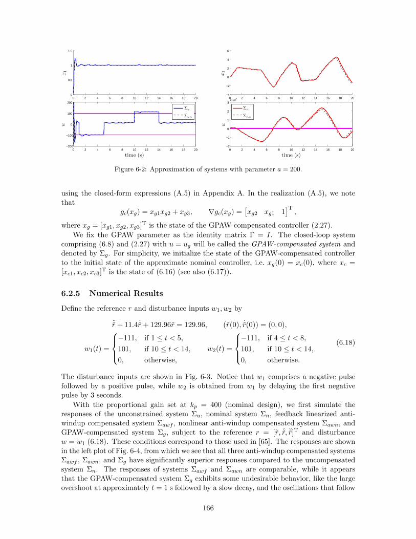
0 2 4 6 8 10 12 14 16 18 200

0.5

1

1.5

x1

0 2 4 6 8 10 12 14 16 18 20−200

−100

0

100

200

u

time (s)

Σu

Σua

0 2 4 6 8 10 12 14 16 18 20−4

−2

0

2

4

6

x1

0 2 4 6 8 10 12 14 16 18 20−2

−1

0

1

2

3x 105

u

time (s)

Σn

Σna

Figure 6-2: Approximation of systems with parameter a = 200.

using the closed-form expressions (A.5) in Appendix A. In the realization (A.5), we notethat

gc(xg) = xg1xg2 + xg3, ∇gc(xg) =[xg2 xg1 1

]T,

where xg = [xg1, xg2, xg3]T is the state of the GPAW-compensated controller (2.27).

We fix the GPAW parameter as the identity matrix Γ = I. The closed-loop systemcomprising (6.8) and (2.27) with u = ug will be called the GPAW-compensated system anddenoted by Σg. For simplicity, we initialize the state of the GPAW-compensated controllerto the initial state of the approximate nominal controller, i.e. xg(0) = xc(0), where xc =[xc1, xc2, xc3]T is the state of (6.16) (see also (6.17)).

6.2.5 Numerical Results

Define the reference r and disturbance inputs w1, w2 by

¨r + 11.4 ˙r + 129.96r = 129.96, (r(0), ˙r(0)) = (0, 0),

w1(t) =

−111, if 1 ≤ t < 5,

101, if 10 ≤ t < 14,

0, otherwise,

w2(t) =

−111, if 4 ≤ t < 8,

101, if 10 ≤ t < 14,

0, otherwise.

(6.18)

The disturbance inputs are shown in Fig. 6-3. Notice that w1 comprises a negative pulsefollowed by a positive pulse, while w2 is obtained from w1 by delaying the first negativepulse by 3 seconds.

With the proportional gain set at kp = 400 (nominal design), we first simulate theresponses of the unconstrained system Σu, nominal system Σn, feedback linearized anti-windup compensated system Σawf , nonlinear anti-windup compensated system Σawn, andGPAW-compensated system Σg, subject to the reference r = [r, ˙r, ¨r]T and disturbancew = w1 (6.18). These conditions correspond to those used in [65]. The responses are shownin the left plot of Fig. 6-4, from which we see that all three anti-windup compensated systemsΣawf , Σawn, and Σg have significantly superior responses compared to the uncompensatedsystem Σn. The responses of systems Σawf and Σawn are comparable, while it appearsthat the GPAW-compensated system Σg exhibits some undesirable behavior, like the largeovershoot at approximately t = 1 s followed by a slow decay, and the oscillations that follow

166

0 2 4 6 8 10 12 14 16 18 20−150

−100

−50

0

50

100

150

time (s)disturban

ceinputs

w1

w2

Figure 6-3: Two disturbance inputs.

0 2 4 6 8 10 12 14 16 18 200

0.5

1

1.5

x1

0 2 4 6 8 10 12 14 16 18 20−200

−100

0

100

200

u

time (s)

Σu

Σn

Σawf

Σawn

Σg

0 2 4 6 8 10 12 14 16 18 200

0.5

1

1.5

x1

0 2 4 6 8 10 12 14 16 18 20−200

−100

0

100

200

u

time (s)

Σu

Σn

Σawf

Σawn

Σg

Figure 6-4: Disturbance response with nominal design, kp = 400. The left plot shows the systemresponses with disturbance input w = w1, while the right plot shows the case withw = w2.

when the disturbance input switches to zero at times t = 5 s and t = 14 s. We will showthat these undesirable phenomena are due to a poor design of the unconstrained system Σu

coupled with the disturbance acting at an inopportune time, i.e. before transients subside.

First, we delay the negative pulse of the disturbance input by 3 seconds, i.e. using thedisturbance input w = w2 (6.18), for which the corresponding responses are shown in theright plot of Fig. 6-4. It can be seen that the slow decay (in the left plot of Fig. 6-4 fort ∈ [1, 5]) is no longer exhibited by system Σg, while the oscillations remain. This showsthat the slow decay is due to the disturbance acting during transients and interacting withthe oscillations at inopportune times.

These oscillations are the natural response of the unconstrained system, as seen from theleft plot of Fig. 6-5, where the closed-loop system is subject to non-zero initial conditionsbut is unforced, i.e. r ≡ 0 and w ≡ 0. The oscillatory behavior is expected because theunconstrained system is poorly damped. This can be seen by inspection of the closed-looppoles. By inspecting the eigenvalues of Acl (6.10), it can be verified that the unconstrainedsystem has a real pole at −198 and a pair of complex conjugate poles at −0.93 ± 5.6i.The dominant complex conjugate poles have natural undamped frequency of 5.7 rad/s and

167

0 0.5 1 1.5 2 2.5 3 3.5 4 4.5 5−2

−1

0

1

2

3

x1

0 0.5 1 1.5 2 2.5 3 3.5 4 4.5 5−500

0

500

u

time (s)

xcl(0) = (1, 0,0)

xcl(0) = (0, 500,0)

xcl(0) = (0, 0,0.2)

0 0.5 1 1.5 2 2.5 3 3.5 4 4.5 5−1

0

1

2

3

x1

0 0.5 1 1.5 2 2.5 3 3.5 4 4.5 5−500

0

500

u

time (s)

xcl(0) = (1, 0,0)

xcl(0) = (0, 500,0)

xcl(0) = (0, 0,0.2)

Figure 6-5: Initial response of unforced unconstrained system, Σu. The left plot shows the case ofnominal design where kp = 400, while the right plot shows the case where kp = 2000.

damping ratio7 of 0.16. Clearly, the unconstrained system Σu is poorly damped. We couldargue that if such poorly damped and oscillatory behavior is acceptable for the unconstrainedsystem, then it must be acceptable for the anti-windup compensated system, in particular,the GPAW-compensated system Σg.

However, the unconstrained system can be better designed by simply increasing theproportional gain kp. In particular, setting kp = 2000 results in superior damping. Withkp = 2000, the closed-loop poles are located at −190 and −5.2±2.6i, with associated naturalundamped frequency of 5.8 rad/s and damping ratio of 0.89. This choice of kp changes thereal pole and natural undamped frequency of the complex poles marginally, while improvingthe damping ratio significantly. The unforced response of the resulting unconstrained systemΣu with non-zero initial conditions is shown in the right plot of Fig. 6-5. The superiorityof this design is clear, and would be a reasonable design for the unconstrained system.

With this new design (kp = 2000), the system responses subjected to the same dis-turbance inputs are shown in Fig. 6-6. The undesirable phenomena exhibited by systemΣg in Fig. 6-4 have been suppressed in Fig. 6-6. Moreover, the response of the GPAW-compensated system Σg has a much shorter rise time when compared to the responses ofsystems Σawf and Σawn. Clearly, the GPAW-compensated system Σg exhibits responsescomparable (or even superior) to those of systems Σawf and Σawn.

Note that we are not advocating the redesign of the nominal controller, but simplyshowing that the relatively poor response of the GPAW-compensated system in Fig. 6-4is due to a poor nominal controller design, rather than inherent weaknesses of GPAWcompensation. The main point is that if the unconstrained system is designed to exhibitoscillatory responses, then it must be acceptable for the GPAW-compensated system toexhibit similar oscillatory responses.

6.3 LMI-based Anti-windup Scheme for Stable LTI Systems

The anti-windup scheme of [128] is a popular method based on the standard anti-windupframework depicted in Fig. 1-1, and applicable to saturated stable LTI systems. One feature

7Recall that for a pair of complex conjugate poles satisfying the equation s2 + 2ζωns + ω2n = 0, the

damping ratio is ζ and the natural undamped frequency is ωn.

168

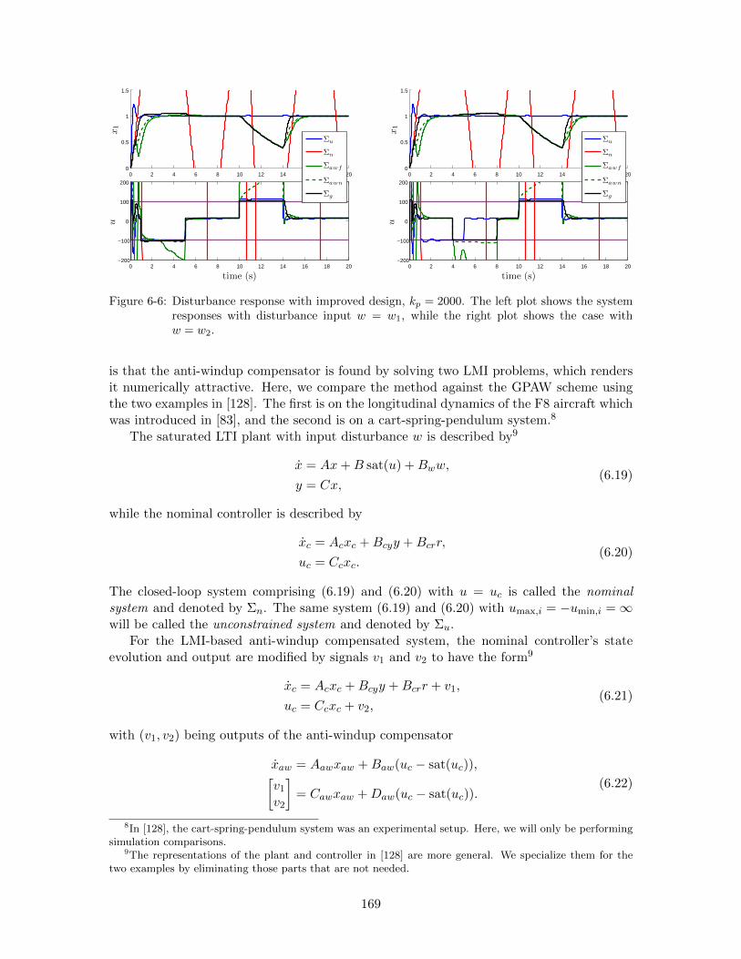
0 2 4 6 8 10 12 14 16 18 200

0.5

1

1.5

x1

0 2 4 6 8 10 12 14 16 18 20−200

−100

0

100

200

u

time (s)

Σu

Σn

Σawf

Σawn

Σg

0 2 4 6 8 10 12 14 16 18 200

0.5

1

1.5

x1

0 2 4 6 8 10 12 14 16 18 20−200

−100

0

100

200

u

time (s)

Σu

Σn

Σawf

Σawn

Σg

Figure 6-6: Disturbance response with improved design, kp = 2000. The left plot shows the systemresponses with disturbance input w = w1, while the right plot shows the case withw = w2.

is that the anti-windup compensator is found by solving two LMI problems, which rendersit numerically attractive. Here, we compare the method against the GPAW scheme usingthe two examples in [128]. The first is on the longitudinal dynamics of the F8 aircraft whichwas introduced in [83], and the second is on a cart-spring-pendulum system.8

The saturated LTI plant with input disturbance w is described by9

x = Ax+B sat(u) +Bww,

y = Cx,(6.19)

while the nominal controller is described by

xc = Acxc +Bcyy +Bcrr,

uc = Ccxc.(6.20)

The closed-loop system comprising (6.19) and (6.20) with u = uc is called the nominalsystem and denoted by Σn. The same system (6.19) and (6.20) with umax,i = −umin,i =∞will be called the unconstrained system and denoted by Σu.

For the LMI-based anti-windup compensated system, the nominal controller’s stateevolution and output are modified by signals v1 and v2 to have the form9

xc = Acxc +Bcyy +Bcrr + v1,

uc = Ccxc + v2,(6.21)

with (v1, v2) being outputs of the anti-windup compensator

xaw = Aawxaw +Baw(uc − sat(uc)),[v1

v2

]= Cawxaw +Daw(uc − sat(uc)).

(6.22)

8In [128], the cart-spring-pendulum system was an experimental setup. Here, we will only be performingsimulation comparisons.

9The representations of the plant and controller in [128] are more general. We specialize them for thetwo examples by eliminating those parts that are not needed.

169

Setting Caw = 0 in (6.22) results in a static anti-windup compensator, for which the stateupdate equation in (6.22) becomes redundant. When Caw 6= 0 and Baw 6= 0, it is a dynamicanti-windup compensator. The closed-loop system comprising (6.19), (6.21), and (6.22)with u = uc will be called the LMI-based anti-windup compensated system and denoted byΣaw. The performance output

z = Czx+Dzu sat(u) +Dzrr, (6.23)

will be needed for the LMI-based anti-windup design [128].

Applying GPAW compensation to the nominal controller (6.20) yields the GPAW-compensated controller (2.27), written as

xg = RI∗(xg, y, r)(Acxg +Bcyy +Bcrr),

ug = Ccxg.(6.24)

Recall that the GPAW-compensated controller can be realized by solving a combinatorialoptimization subproblem (2.31), a convex quadratic program (4.12), or a projection onto aconvex polyhedral cone problem (see Section 4.1). Moreover, closed-form expressions areavailable when the controller output is of dimension one or two (see Appendices A and B).The closed-loop system (6.19) and (6.24) with u = ug will be called the GPAW-compensatedsystem and denoted by Σg.

6.3.1 Longitudinal Dynamics of the F8 Aircraft

The saturated longitudinal dynamics of the F8 aircraft [83] is described by (6.19), saturationlimits umax,i = −umin,i = 25 (deg) for i ∈ 1, 2, and matrices

A =

−0.8 −0.0006 −12 0

0 −0.014 −16.64 −32.21 −0.0001 −1.5 01 0 0 0

, B =

−19 −3−0.66 −0.5−0.16 −0.5

0 0

,C =

[0 0 0 10 0 −1 1

], Bw = 0.

The outputs y = [y1, y2]T = Cx represent the aircraft pitch angle and flight path an-gle respectively, both in degrees. The inputs u = [u1, u2]T represent the elevator angleand flaperon angle respectively, both also in degrees. The nominal controller is describedby (6.20) and matrices [83, 128]

Ac =

[Aa +BaG−HCa 0

G 0

], Bcy = −Bcr =

[H0

], Cc =

[0 I

], (6.25)

Aa =

[0 0B A

], Ba =

[I0

], Ca =

[0 C

],

G =

[−52.23 −3.36 73.1 −0.0006 −94.3 1072−3.36 −29.7 −2.19 −0.006 908.9 −921

],

H =

[−0.844 −11.54 −0.86 −47.4 4.68 4.820.819 13.47 0.25 15 −4.8 0.14

]T

.

170

LMI-Based Anti-windup Compensated System

We use the anti-windup synthesis procedure [128, Procedure 1] to design four anti-windupcompensators10 as in the F8 aircraft example in [128]. The first two correspond to a staticdesign and plant-order dynamic anti-windup design for the performance output z = y − r(see (6.23)).

Remark 6.3. When following [128, Procedure 1], there are two somewhat arbitrary imple-mentation decisions that may change the resultant anti-windup compensator gain matrices.Here, we state the choices made so that results can be reproduced in the same manner.

The first is on the decomposition of the matrix N := NNT where the rectangular matrixN is sought (see equation (16) in [128]). Since N = NT, it has a special eigendecompo-sition N = Qdiag(λ1, λ2, . . . , λn)QT [124, Corollary 2.5.14, pp. 107 – 108] where λi arethe eigenvalues and Q has the associated eigenvectors as its columns and is orthogonal,i.e. QT = Q−1. This decomposition can be easily found by the MATLAB R© function eig.We choose N to be composed of the columns of Q corresponding to nonzero eigenvalues,each multiplied by the square root of the associated eigenvalue, i.e. if λi 6= 0, then the i-thcolumn of Q multiplied by

√λi is a column of N . It can be verified that N constructed as

such is a full rank matrix satisfying N = NNT.

The second implementation choice is on the parameters δ > 0 and Vs [128, Procedure 1,Step 4]. We choose δ = 1 and Vs = I, so that U = δV −1

s = I.

Following [128, Procedure 1] to design a static anti-windup compensator for the perfor-mance output z = y − r yields the matrix Daws1 ∈ R10×2 with numeric values11

Daws1 =

[−6.0630 −10.002 5.2920 1277.8 0.18403 −0.89916 −6.202368.949 −328.39 133.85 19621 8.4154 −10.969 66.795

−10.954 0.90498 −1.5567−344.53 −2.0689 −34.401

]T

.

The static anti-windup compensator is (6.22) with Aaw = 0, Baw = 0, Caw = 0, andDaw = Daws1. The resulting LMI-based anti-windup compensated system will be denotedby Σaws1.

For the same performance output z = y−r, the plant-order dynamic anti-windup designis defined by matrices

Aawd1 =

−0.95591 −139.50 −136.67 231.64−2.4906 −363.48 −356.11 554.51−1.7471 −255.25 −250.17 −824.850.15826 11.696 7.9575 −46478

× 104,

10The numerical values for the matrices defining the dynamic anti-windup compensators were not listedin [128]. While the matrices Λ4 given (at the bottom of [128, pp. 1517 – 1518]) are supposed to define thestatic anti-windup compensators, the responses obtained do not agree with those in [128, Figs. 6 and 7].The designs obtained by following [128, Procedure 1] produces systems whose responses agree with thosein [128, Fig. 6 and 7].

11The numeric values of the anti-windup gain matrices as presented are rounded to 5 significant digits,and listed only for verification purposes. The values used in simulations are in full resolution obtainedthrough [128, Procedure 1].

171

Bawd1 =

−342.43 −6143.4−892.43 −16007−630.55 −11219−118.73 1346.8

× 104,

Cawd1 =

−0.00099418 −0.042736 −0.042250 0.0519710.013053 −0.33842 −0.38844 0.985430.019578 −0.25296 −0.34722 0.81876−0.010485 0.15023 0.56599 −1.04970.0028824 0.024005 −0.0045734 −0.024250−0.0048033 0.028520 0.0050051 −0.0522200.000061898 −0.038441 −0.044896 0.061231

0.030087 −0.26891 −0.41181 1.0855−12.876 −1883.4 −1846.5 −14849−231.53 −33781 −33093 81270

× 102,

Dawd1 =

−0.0015596 −0.0089517−0.0068185 −0.13679−0.0042489 −0.0774360.0067893 0.11487−0.000057559 −0.00047552

0.00019815 0.0045669−0.0015658 −0.0090705−0.0068035 −0.13682−46.803 −826.22−828.45 −14882

× 104.

Specifically, it is given by (6.22) with Aaw = Aawd1, Baw = Bawd1, Caw = Cawd1, andDaw = Dawd1. The resulting LMI-based anti-windup compensated system will be denotedby Σawd1.

To improve the performance, anti-windup compensators were designed for the perfor-mance output defined by (6.23) and matrices

Cz =

[0 0 0 3

4−0.8 −0.0006 −12 0

], Dzu = 0, Dzr =

[−3

4 00 0

]. (6.26)

The matrix Daws2 ∈ R10×2 that defines the static design is given by

Daws2 =

[−14.312 55.098 0.10642 4.8030 −0.014923 −0.3018776.652 −526.75 −2.3909 −30.136 −0.52966 −0.69344

−14.379 55.009 0.97391 0.02358976.354 −525.43 0.13938 0.71856

]T

,

where the static anti-windup compensator is (6.22) with Aaw = 0, Baw = 0, Caw = 0, andDaw = Daws2. The resulting LMI-based anti-windup compensated system will be denotedby Σaws2.

For the same performance output defined by (6.23) and (6.26), the plant-order dynamic

172

anti-windup design is defined by matrices

Aawd2 =

0.067552 3.3508 −358.69 −162.76−2.6410 −129.22 14044 3711.32.1302 99.123 −11388 4604.2

0.0013977 33.404 386.35 −49636

× 104,

Bawd2 =

135.12 −902.07−5278.1 352614244.6 −2842485.749 −129.26

× 104,

Cawd2 =

0.0000058254 0.00032522 0.0016350 0.0039970−0.00011178 −0.0017618 −0.0092329 −0.023160−0.000062008 −0.000068350 0.00011921 −0.000079288−0.0037391 0.0040623 −0.0093207 −0.00516650.000052263 −0.00019850 0.00016987 0.0000201330.00046070 −0.00037181 −0.00049672 −0.0000975640.000019729 0.00030590 0.0016650 0.0039889−0.00010796 −0.0019326 −0.0084796 −0.022410−0.54861 −26.871 2917.0 814.51

3.6685 176.71 −19541 −1024.4

× 103,

Dawd2 =

−0.0072343 −0.00699480.0058178 −0.0190800.00053019 −0.00163560.00065605 −0.026219−0.00056711 0.0013408−0.00046369 0.00012203−0.0072424 −0.00718880.0058214 −0.022481−1096.5 7324.77324.6 −48969

× 103.

Specifically, it is given by (6.22) with Aaw = Aawd2, Baw = Bawd2, Caw = Cawd2, andDaw = Dawd2. The resulting LMI-based anti-windup compensated system will be denotedby Σawd2.

GPAW-Compensated System

Because the stability results obtained thus far are too conservative to be applied to thissystem,12 we use an ad hoc method (optimizing over the time response for a specific ref-erence) to determine the GPAW parameter Γ. As shown in the next section, the resultantGPAW-compensated system exhibits reasonable responses for some reference inputs it wasnot optimized for.

First, we show that for the GPAW-compensated controller (6.24) defined by (6.25),only 15 elements among the 64 in Γ ∈ R8×8 are significant while the remaining 49 areredundant or implicitly defined. From (6.25), we have Cc =

[0 I

]= [e7, e8]T, where

12Specifically, the nominal controller is only marginally stable and Theorem 5.2.1 requires both the plantand controller to be strictly stable (see Remark 5.1) and hence not applicable.

173

ei ∈ R8 for i ∈ I8 are standard basis vectors in R8. Partition Γ = ΓT as Γ =[

Γ11 Γ12

ΓT12 Γ22

],

where Γ12 ∈ R6×2 and Γ22 ∈ R2×2. From the closed-form expressions (B.5) in Appendix B,we see that Γ is always post-multiplied by either the gradient vectors ∇gc1 = e7, ∇gc2 = e8,or the matrix N = CT

c = [e7, e8]. Such multiplications eliminate the first 6 columns ofΓ, so that Γ11 ∈ R6×6 can never affect the GPAW-compensated controller, rendering itredundant. Hence the GPAW-compensated controller is fully defined by Γ12 (12 elements)and Γ22 = ΓT

22 (3 independent elements), i.e. 15 elements in total.

Since Γ11 is redundant, we can choose it to be Γ11 = αI6 for some α > 0, so that

Γ =[αI6 Γ12

ΓT12 Γ22

]. Observing that Γ > 0 if and only if Γ22 >

1αΓT

12Γ12 [124, Theorem 7.7.6,

p. 472], we see that Γ > 0 when Γ22 = ΓT22 > 0 and α > 0 is chosen sufficiently large. Hence

to enforce Γ > 0, the only constraint we need to impose is Γ22 > 0. For simplicity, we fixΓ22 = I2 > 0, so that the 12 elements of Γ12 can be chosen arbitrarily.

We determine Γ by optimizing the time response of the GPAW-compensated system tothe step reference r = [r1, r2]T = [15, 15]T for all t ≥ 0 (see (6.24)), and with zero initialconditions. Specifically, we solve the unconstrained minimization problem13

minΓ12∈R6×2

F (Γ12) =

∫ 3

050(y1(t)− r1)2 + (y2(t)− r2)2 dt,

where y(t) = [y1(t), y2(t)]T for t ∈ [0, 3] is the plant output (dependent on Γ) obtainedfrom simulation, and we have fixed Γ22 = I2 to simplify the optimization problem. Asshown above, for any choice of Γ12, there exists a Γ11 such that Γ > 0, which leads toan unconstrained optimization problem. The preceding optimization problem was solvedusing the nonlinear program solver fminunc of the MATLAB R© Optimization Toolbox [186],

which yields Γ =[αI6 Γ12

ΓT12 I2

]with

Γ12 =

[0.0016116 −0.0014137 0.027579 −0.00000026455 −0.054469 0.29149−0.32659 −0.93800 0.77329 −0.00018794 0.73616 0.052871

]T

.

Numerical Results

The systems Σu, Σn, Σaws1, Σawd1, Σaws2, Σawd2, and Σg are first simulated for the stepreference r = [10, 10]T for all t ≥ 0. Notice that the GPAW-compensated system was notoptimized for this reference. The responses for systems Σu, Σn, Σaws1, Σawd1, and Σg areshown in Fig. 6-7, while those of Σu, Σn, Σaws2, Σawd2, and Σg are shown in Fig. 6-8.

Observe from Fig. 6-7 that when designed for the nominal performance output z =y−r, the LMI-based anti-windup compensated systems Σaws1, Σawd1 exhibit some overshootin their output y1. In contrast, the GPAW-compensated system exhibits a superior welldamped response. Notice that controller state-output consistency (see Theorem 2.5.3) holdsonly14 for the GPAW-compensated system Σg, which is also evident in Figs. 6-8 and 6-9.

To reduce the overshoot of the LMI-based anti-windup designs, the performance outputwas modified to (6.23), (6.26), yielding systems Σaws2 and Σawd2 [128]. Fig. 6-8 shows this

13The weighting of 50 in the objective function was chosen to reduce overshoots, so that the GPAW-compensated system exhibits responses comparable to those of the LMI-based anti-windup scheme.

14Results shown in [128, Figs. 6 and 7] for the control signals are with additional saturation applied,which is conventional in the anti-windup literature. The control signals shown in Figs. 6-7, 6-8, and 6-9, arewithout the additional saturation.

174

−1 0 1 2 3 4 50

5

10

15

y 1

−1 0 1 2 3 4 50

5

10

15

y 2

time (s)

−1 0 1 2 3 4 5−30

−20

−10

0

u1

−1 0 1 2 3 4 5−10

0

10

20

30

u2

time (s)

Σu

Σn

Σaws1

Σawd1

Σg

Figure 6-7: Step response for F8 aircraft longitudinal dynamics, nominal case.

−1 0 1 2 3 4 50

5

10

15

y 1

−1 0 1 2 3 4 50

5

10

15

y 2

time (s)

−1 0 1 2 3 4 5−30

−20

−10

0

u1

−1 0 1 2 3 4 5−10

0

10

20

30

u2

time (s)

Σu

Σn

Σaws2

Σawd2

Σg

Figure 6-8: Step response for F8 aircraft longitudinal dynamics, with modified performance outputfor LMI-based anti-windup scheme.

modification to be effective in eliminating the overshoots in the output y1. The response ofthe GPAW-compensated system Σg in Fig. 6-8 remains unchanged from Fig. 6-7. Clearly,responses of systems Σg and Σaws2, Σawd2 are comparable (with the modified performanceoutput), and are significant improvements over the uncompensated system Σn.

The GPAW parameter Γ was determined by optimizing for the reference input, r =[15, 15]T for all t ≥ 0, the response of which is shown in Fig. 6-9. Clearly, the response ofthe GPAW-compensated system is qualitatively similar to those in Figs. 6-7 and 6-8 (withreference input r = [10, 10]T for all t ≥ 0), cases for which it was not optimized for. Thissuggests that satisfactory responses can be expected of the GPAW-compensated system forat least a class of reference inputs.

6.3.2 Cart-Spring-Pendulum System

The other example used to demonstrate the effectiveness of the anti-windup scheme pro-posed in [128] is an experimental cart-spring-pendulum system, described by (6.19), satu-

175

−1 0 1 2 3 4 50

5

10

15

20

y 1

−1 0 1 2 3 4 50

5

10

15

20

y 2

time (s)

−1 0 1 2 3 4 5−30

−20

−10

0

u1

−1 0 1 2 3 4 5−10

0

10

20

30

40

u2

time (s)

Σu

Σn

Σaws2

Σawd2

Σg

Figure 6-9: Step response for F8 aircraft longitudinal dynamics, with large step input.

ration limits umax = −umin = 5 (V), and matrices

A =

0 1 0 0

−330.46 −12.15 −2.44 00 0 0 1

−812.61 −29.87 −30.10 0

, B =

0

2.717620

6.68268

,C =

[1 0 0 00 0 1 0

], Bw =

[0 0 0 15.61

]T.

(6.27)

The outputs y = [y1, y2]T = Cx represent the cart’s displacement (in meters) from equilib-rium and pendulum angle (in radians) from the downward vertical respectively. The inputu represent the motor input in Volts. The nominal controller is described by (6.20) andmatrices

Ac = A−BK − LC, Bcy = L, Bcr = 0, Cc = −K,

K =[64.81 213.12 1242.27 85.82

], L =

[64 2054 −8 −1432−8 −280 142 10169

]T

.(6.28)

LMI-Based Anti-windup Compensated System

In contrast to Section 6.3.1, the LMI-based dynamic anti-windup compensator (6.22) definedby matrices

Aaw =

−65.02 198.43 98.11 −66.75223.94 −697.09 −347.39 247.2441.17 −98.10 −47.56 55.25−121.39 309.97 138.31 −131.52

, Baw =

0.0688−0.2620−0.06370.1559

,

Caw =

41.22 −160.42 −106.41 82.03−3469.09 8318.57 3423.87 −2388.49−162.51 386.26 −35.56 71.07−4584.37 9490.06 −11350.16 11407.08

587.11 −1687.16 −821.25 632.86

, Daw =

−0.06222.90700.23385.5623

0

,

176

in [128], does reproduce the results in [128, Figs. 9 and 10]. As mentioned in [128], theconditions to construct static anti-windup compensators are infeasible.

GPAW-Compensated System

It can be verified that both the open-loop plant (6.19), (6.27), and the nominal control-ler (6.20), (6.28), are strictly stable. However, condition (5.10) was found to be numericallyinfeasible, so that Theorem 5.2.1 cannot be applied. This again suggests conservatism ofTheorem 5.2.1. Without a systematic mechanism to determine the GPAW parameter Γ, weuse an ad hoc method as before.

We will be optimizing some measure of system performance over Γ for a specified distur-bance input, similar to the approach in Section 6.3.1. First, we show that we can completelydefine the GPAW-compensated controller (6.24) using only 3 elements of Γ = ΓT ∈ R4×4.Using a modified Gram-Schmidt orthonormalization process [124, pp. 15 – 16], a nonsingulartransformation matrix

T =

[CcT

]=

−64.81 −213.12 −1242.27 −85.821263.3 −10.933 −63.729 −4.4026

0 1246.9 −212.89 −14.7070 0 −87.182 1262.0

,was found, that transforms the nominal controller (6.20), (6.28), into

˙xc = Acxc + Bcyy = TAcT−1xc + TBcyy,

uc = Ccxc = CcT−1xc =

[1 0 0 0

]xc,

(6.29)

with the special form of Cc (see also Section 5.5.1). Then from the closed-form expres-sions (A.7) (in Appendix A) for the GPAW-compensated controller derived from the trans-formed nominal controller (6.29), we see that Γ = [γij ] appears only in the projectionmatrix, which, due to the special structure of Cc, can be simplified to

I − ΓCTc Cc

CcΓCTc

= I − 1

γ11

γ11 0 0 0γ21 0 0 0γ31 0 0 0γ41 0 0 0

=

0 0 0 0−γ21γ11

1 0 0

−γ31γ11

0 1 0

−γ41γ11

0 0 1

:=

0 0 0 0γ1 1 0 0γ2 0 1 0γ3 0 0 1

,with γ1 := −γ21

γ11, γ2 := −γ31

γ11, and γ3 := −γ41

γ11. Clearly, the resultant GPAW-compensated

controller is fully defined by the 3 parameters in γ := [γ1, γ2, γ3]T. Note that the remainingelements of Γ can always be defined in a way to ensure Γ is symmetric positive definite, sothat no restrictions need to be imposed on γ.

The GPAW-compensated controller derived from the transformed nominal controller (6.29)is given by

˙xg = RI∗(xg, y)(Acxg + Bcyy),

ug = Ccxg.(6.30)

As before, we call the resultant closed-loop system comprising (6.19) and (6.30) with u = ugthe GPAW-compensated system and denote it by Σg. To determine γ (and hence Γ), we

177

optimize (over γ) the time response of Σg to the disturbance input (see (6.19))

w =

1.588, if t ∈ [0, 0.01],

0, otherwise.(6.31)

Specifically, we solve the unconstrained minimization problem

minγ∈R3

F (γ) =

∫ 8

0y2

1(t) dt,

where y(t) = [y1(t), y2(t)]T for t ∈ [0, 8] is the plant output (dependent on Γ) obtainedfrom simulation. The preceding unconstrained optimization problem was solved using thenonlinear program solver fminunc of the MATLAB R© Optimization Toolbox [186], whichyields a satisfactory solution

γ =[−0.21853 −4.9972 −3.9991

]T,

when started with the initial guess γig = [−0.2,−5,−4]T.

Remark 6.4. Numerical experience indicates that the posed optimization problem is poorlyscaled, i.e. the objective is highly sensitive to γ1 while being relatively insensitive to γ2 andγ3. The optimization was solved repeatedly with numerous initial guesses, and the initialguess γig = [−0.2,−5,−4]T was found to yield a satisfactory solution.

Numerical Results

The systems Σu, Σn, Σaw, and Σg are first simulated for the nominal disturbance in-put (6.31). The responses are shown in the left plot of Fig. 6-10. It can be seen that

0 2 4 6 8 10

−0.05

0

0.05

y 1

0 2 4 6 8 10−0.4

−0.2

0

0.2

y 2

0 2 4 6 8 10

−5

0

5

u

time (s)

Σu

Σn

Σaw

Σg

0 2 4 6 8 10

−0.05

0

0.05

y 1

0 2 4 6 8 10−0.4

−0.2

0

0.2

y 2

0 2 4 6 8 10

−5

0

5

u

time (s)

Σu

Σn

Σaw

Σg

Figure 6-10: Response of cart-spring-pendulum system to disturbances. The left plot shows thecase for nominal disturbance while the right plot shows the case where the nominaldisturbance is magnified by 50%.

without anti-windup compensation, the response of system Σn is highly oscillatory with alarge settling time of approximately 10 s. The response of the GPAW-compensated sys-tem Σg is comparable to that of the LMI-based anti-windup compensated system Σaw,although Σaw exhibits a marginally superior response. Both responses of systems Σg and

178

Σaw are significantly superior to the response of the uncompensated system Σn, reachingsteady state at approximately 5 s. Observe also that controller state-output consistency(see Theorem 2.5.3) holds for the GPAW-compensated system Σg, but not for system Σaw.

Since the GPAW parameter Γ was determined by optimizing for a specific disturbanceinput, namely (6.31), we check its performance against a disturbance which is 50% largerin magnitude. The responses to the increased excitation are shown in the right plot ofFig. 6-10. Clearly, the GPAW-compensated system Σg exhibits satisfactory responses todisturbance inputs for which it was not optimized for.

6.4 Chapter Summary

We compared the GPAW scheme against three state-of-the-art anti-windup schemes usingexamples available from the literature. Because the stability results obtained thus far are tooconservative to be applied, stability of the GPAW-compensated systems are not established.Even in the absence of stability results, ad hoc methods can be devised to design theGPAW-compensated controller. We showed that the GPAW scheme achieves comparableperformance against these state-of-the-art anti-windup schemes in these examples. Wherecurrent stability results are not applicable, the GPAW scheme provides practitioners witha candidate anti-windup scheme where no candidates may be available otherwise.

179

180

Chapter 7

Conclusions and Future Work

Windup induced by control saturation remains one of the major problems affecting vir-tually all practical control systems, with adverse consequences. The gradient projectionanti-windup (GPAW) scheme proposed in this dissertation is a general purpose anti-windupscheme constructed for saturated nonlinear systems driven by nonlinear controllers, a topicrecognized as a largely open problem. The GPAW-compensated controller achieves control-ler state-output consistency, possesses clear geometric properties, and is characterized by apassive projection operator. It is defined by either the online solution to a combinatorialoptimization subproblem, a convex quadratic program, or a projection onto a convex poly-hedral cone problem. When the controller output has dimension one or two, closed-formexpressions for the GPAW-compensated controller are available.

Strong results were obtained when GPAW compensation is applied to saturated first-order LTI plants driven by first-order LTI controllers. This simple system illustrates nu-merous attractive features of the GPAW scheme. For this system, GPAW compensationcan only maintain/enlarge the ROA of the uncompensated system, a result independent ofany Lyapunov function. Qualitative weaknesses of some existing anti-windup results weredemonstrated. This motivates a new paradigm to address the anti-windup problem, whereresults relative to the uncompensated system are sought. Numerical results further suggesta need to consider asymmetric saturation constraints for general saturated systems, whichhas been largely ignored in the literature.

We derived some ROA comparison and stability results for GPAW-compensated MIMOnonlinear and MIMO LTI systems. These ROA comparison results represent the first stepsconsistent with the new anti-windup paradigm. We note that these ROA comparison resultsstate explicit advantages of adopting GPAW compensation. This is in contrast to someexisting anti-windup results where the purported advantages offered by the anti-windupscheme may be achieved by the uncompensated system.

Stability results obtained thus far are still fairly conservative. By means of non-trivialexamples available in the literature, we showed that even in the absence of applicable sta-bility results, ad hoc methods can still be devised to design GPAW-compensated controllerswith performance comparable to some state-of-the-art anti-windup schemes. Where currentstability results are not applicable, the general purpose GPAW scheme provides practition-ers with a candidate anti-windup scheme endowed with some attractive properties.

The significance of the research presented herein has to be seen in a larger context. Con-sider the standard anti-windup structure depicted in Fig. 1-1. This anti-windup structureis essentially a generalization of that adopted in [187], which in turn is inspired by the back-

181

calculation method [53]. Apart from the fact that this structure preserves the unconstrainedresponse when the saturation constraints are not triggered,1 it has no attractive inherentproperties. All performance and stability properties of the anti-windup compensated sys-tem are intimately dictated by the anti-windup gains. Numerous anti-windup schemes havesince been developed based on this anti-windup structure, differing only in the assump-tions imposed and method of determining the anti-windup gains [14]. Even state-of-the-artanti-windup schemes for nonlinear systems like [24, 65] adopted variants of the standardanti-windup structure of Fig. 1-1.

In contrast to the standard anti-windup structure, the GPAW scheme has several addi-tional “built-in” features (mentioned above) induced by the projection operator, and is de-fined by a single symmetric positive definite matrix parameter. In essence, the projection op-erator has endowed the GPAW-compensated controller much of its inherent properties, andthe GPAW parameter is only meant to allow some “fine tuning”.2 The fact that the singleunified structure of the GPAW scheme can achieve comparable performance as three state-of-the-art anti-windup schemes adopting variants of the standard anti-windup structureshows the versatility of the GPAW scheme. Moreover, these state-of-the-art anti-windupschemes cannot be applied to the simple system (4.42) used in Section 4.5.2 to demonstratethe application of the ROA comparison result, Theorem 4.4.1 (see Remark 4.11). Theseshow the potential for the GPAW scheme to be developed into a truly general purposeanti-windup scheme with stability guarantees.

The research presented herein represents the first steps in the study of GPAW compen-sation. We invite the reader to join us in this quest to solve one of the most prevalentproblems affecting control systems, in a journey that promises to be theoretically rich andpractically important.

7.1 Future Work

Given the conservativeness of current stability results, there is a need to develop less con-servative results for the GPAW scheme.3 Apart from this obvious line of research, potentialwork that have been identified are listed below.

7.1.1 Robustness Issues due to Presence of Noise, Disturbances, TimeDelays, and Unmodeled Dynamics

Apart from control saturation, practical control systems are adversely affected by the pres-ence of noise, disturbances, time delays, and unmodeled dynamics. Recognizing that anti-windup compensation for nonlinear systems is still largely an open problem, we have chosento ignore these important issues with regard to GPAW-compensated systems. Addressingthese will become increasingly important as research in GPAW compensation matures.

1The state of the anti-windup compensator has to be appropriately initialized for this to hold.2Indeed, for first order nominal controllers, the GPAW-compensated controller is independent of any

GPAW parameters (see Remark B.1 in Appendix B).3In this regard, we note that the GPAW parameter may be allowed to vary with the controller state,

measurement, or reference input, and the objective function of the associated combinatorial optimizationsubproblem may be modified.

182

7.1.2 Robustness Issues due to Different Realizations of Anti-windupCompensator Derived from Anti-windup Compensated Controller

If an anti-windup compensator is needed, perhaps because the nominal controller cannotbe modified, it was shown in Section 1.3.1 how it can be derived from an associated anti-windup compensated controller. There are numerous ways to do so, and each realizationwill vary in its robustness properties. One area of possible research is to study the methodsto realize the anti-windup compensator with satisfactory robustness properties.

7.1.3 Verify if Reference Governors Solves General Anti-windup Problem

In Section 1.4.6, reference governors [23, 95–99] have been identified as a likely candidate tosolve Problem 1 (see Section 1.3). At this point, due to the literature on reference governorsadopting a different problem statement, it is uncertain whether it indeed solves Problem 1,or whether it can be modified such that it does so. There is a need to examine the literatureon reference governors to confirm this.

7.1.4 Continuous Time Gradient Projection Method as a Valid Optimiza-tion Method

In Section 2.3, we extended Rosen’s gradient projection method to continuous time withthe intention of extracting only the resultant projection operator. We attempted to showthat the extension is correct by means of a numerical example, without proving that itindeed solves the underlying optimization problem. Since continuous optimization is anactive research field, study of the continuous time extension may contribute to this area.

7.1.5 Exploit Projection Operator

The projection operator was extracted from the continuous time gradient projection methodin Section 2.4, for the purpose of constructing the GPAW-compensated controller. Clearly,it can be used for other purposes, e.g. to bound parameter estimates in adaptive control4

as in [122, Sections 4.4, 8.4.2, and 8.5.5], and more general constrained control (see Sec-tion 2.8.3). Moreover, since the projection operator induces a “sliding” motion on thesaturation constraint boundaries (e.g. see Figs. 2-2 and 3-4), it may possibly be used fruit-fully in sliding mode control [38, Chapter 7, pp. 276 – 310].

7.1.6 GPAW-Compensated Systems in Relation to Projected DynamicalSystems

As shown in Section 3.2, the GPAW-compensated system obtained by applying GPAWcompensation to the simple system considered is in fact a projected dynamical system(PDS) [107–110]. PDS is a significant line of independent research that has attractedthe attention of mathematicians, physicists, and economists, among others. It is likely thatGPAW-compensated systems are closely related to PDS. Establishing a concrete link be-tween general GPAW-compensated systems and PDS will allow cross utilization of ideasand methods, among other strategic benefits. To this end, we note that results in [151] maybe useful.

4In fact, the GPAW scheme was inspired by the projection mechanism used in adaptive control.

183

7.1.7 Passivity and Small-Gain Based Stability Results

We showed in Section 2.7 that the GPAW-compensated system is obtained by modifying theuncompensated system with a passive projection operator (with L2-gain less than one) andtwo transformation matrices (see Fig. 2-5). Some possible research would be to exploit theseproperties to derive passivity and small-gain-based stability results for GPAW-compensatedsystems (see [37, Theorem 5.6, p. 218, Section 6.5, pp. 245 – 259]).

7.1.8 Show Performance Improvement and Prove Conjectures for PlanarLTI Systems

In Section 3.8, we attempted to show that the GPAW scheme solves Problem 1 (in Sec-tion 1.3). As explained in Remark 3.20, verifying that performance is improved by GPAWcompensation is a non-trivial task. This needs to be studied, as well as proving or disprovingConjectures 3.1 and 3.2. See possible hints following the statements of these conjectures.

7.1.9 Existence and Uniqueness of Solutions to General GPAW-CompensatedSystems

Existence and uniqueness of solutions are fundamental properties required for a meaningfulstudy of dynamic systems. For the planar LTI system studied in Chapter 3, these are assuredby Proposition 3.3.3. For GPAW-compensated MIMO LTI systems that are equivalent tolinear systems with partial state constraints (see Section 5.6), existence and uniqueness ofsolutions are established in [103]. We need to establish these properties for general GPAW-compensated systems. To this end, if GPAW-compensated systems can be shown to beequivalent to PDS [107–110], then [107, Theorem 2] can be used to assert existence anduniqueness of their solutions, as demonstrated in the proof of Proposition 3.3.3. A moregeneral approach is to use results from the theory of differential equations with discontinuousright-hand sides [120]. In particular, results in [120, §2.7, pp. 75 – 86, and §2.10, pp. 106 –117] may be useful.

7.1.10 Effects of Controller State Augmentation and Redundant Satura-tion Constraints

In Remark 2.23, we cautioned against indiscriminate controller state augmentation whenattempting to obtain an approximation of the nominal controller. This is closely related tohaving redundant saturation constraints as discussed in Section 5.5.3. Observe that theseissues are also present in the standard anti-windup framework of Fig. 1-1. However, to thebest of our knowledge, these issues have not been addressed in the literature. These aspectsare poorly understood and their study may allow more effective exploitation of availablecontrol authority.

184

Appendix A

Closed Form Expressions forSingle-outputGPAW-Compensated Controllers

Single-output controllers1 abound in practice. Here, we show how closed-form expressionscan be obtained for single-output GPAW-compensated controllers by analyzing the asso-ciated combinatorial optimization subproblem, which allows a highly efficient realization(see Section B.1 in Appendix B for computational results when the controller output isof dimension two). These demonstrations also show that such controllers reduces to thoseobtained by the conditional integration method (see Section 2.1). In fact, the hybrid natureof general GPAW-compensated controllers are made evident due to the switching structureexposed here (as well as in Appendix B). The closed-form expressions are first derived forsingle-output nonlinear controllers, and then specialized to LTI controllers. We concludethis appendix with the closed-form expressions for GPAW-compensated approximate PIDcontrollers, since they represent an important subclass.

Consider the single-output nominal controller (2.26)

xc = fc(xc, y, r), xc(0) = xc0,

uc = gc(xc),(A.1)

with the restriction that uc is scalar. Here, (xc, y, r) ∈ Rq × Rp × Rnr are of finite butotherwise arbitrary dimensions. For controllers of general structure (1.3), it was shown inSection 2.6 that an arbitrarily close approximating controller having the form of (A.1) canbe constructed. Following the development in Section 2.5, the derived GPAW-compensatedcontroller has the form (2.27)

xg = RI∗(xg, y, r)fc(xg, y, r), xg(0) = xc0,

ug = gc(xg),(A.2)

where ug ∈ R. The scalar saturation constraint umin ≤ ug ≤ umax is equivalent to the twoconstraints

h1(xg) = gc(xg)− umax ≤ 0, h2(xg) = −gc(xg) + umin ≤ 0,

1Clearly, single-output controllers include SISO controllers.

185

where the gradients of h1 and h2 are

∇h1(xg) = −∇h2(xg) = ∇gc(xg).

Define the index set of active saturation constraints, and the candidate solution set2

Isat := Isat(xg) = i ∈ I2 | hi(xg) ≥ 0, J := I ⊂ Isat | |I| ≤ q.

Observe that the two constraints h1(xg) ≤ 0, h2(xg) ≤ 0, cannot be simultaneously active,so that Isat can only be ∅, 1, or 2. Then the candidate solution set J for each of thesecases maps according to3

(Isat = ∅)⇒ (J = ∅), (Isat = 1)⇒ (J = ∅, 1),(Isat = 2)⇒ (J = ∅, 2).

Since I ∈ J implies I ∈ ∅, 1, 2, we only need to define NI(xg) (2.29) as the q × 1matrix4

NI(xg) =

∇h1(xg), if I = 1,∇h2(xg), if I = 2,0, otherwise,

or NI(xg) =

∇gc(xg), if I = 1,−∇gc(xg), if I = 2,0, otherwise,

for any I ∈ ∅, 1, 2. Choose some Γ = ΓT > 0 ∈ Rq×q as the GPAW parameter. If∇gc(xg) 6= 0 ∈ Rq and I ∈ ∅, 1, 2, the projection matrix (2.30) can be written as

RI(xg) =

I − Γ∇gc∇Tgc(xg)

∇TgcΓ∇gc(xg), if I 6= ∅,

I, otherwise,(A.3)

since ΓNI(NTI ΓNI)

−1NTI (xg) = Γ∇gc(∇TgcΓ∇gc)−1∇Tgc(xg) =

Γ∇gc∇Tgc(xg)∇TgcΓ∇gc(xg)

, for I ∈1, 2.

The single-output GPAW-compensated controller (A.2) is defined by (A.3) and a solu-tion I∗ to the combinatorial optimization subproblem (2.31), reproduced below

maxI∈J

F (I) = fTc (xg, y, r)Γ

−1RI(xg)fc(xg, y, r),

subject to rank(NI(xg)) = |I|,NTIsat(xg)RI(xg)fc(xg, y, r) ≤ 0.

(A.4)

What follows is a detailed analysis of subproblem (A.4) to extract the closed form expres-sions for the single-output GPAW-compensated controller (A.2).

For notational convenience, we will drop all function arguments. Due to Proposi-tion 2.5.2, I = ∅ is an optimal solution whenever it is feasible (see also Remark 2.17).Clearly, I = ∅ satisfies the first constraint of subproblem (A.4). It will be infeasible onlywhen it fails to satisfy the second constraint. This happens only when

(i) Isat = 1 and NTIsatR∅fc = ∇Tgcfc > 0; or

2Recall that Ii := 1, 2, . . . , i for any positive integer i.3Note that ⇒ denotes logical implication.4Notice that the bijection σI described in Remark 2.5 is not needed for this case.

186

(ii) Isat = 2 and NTIsatR∅fc = −∇Tgcfc > 0.

When condition (i) holds, we have ∇Tgc 6= 0 (due to ∇Tgcfc 6= 0), which implies the firstconstraint of subproblem (A.4) is satisfied for I = 1. From (A.3), it can be verified thatNTIsatRI = 0 for I = 1, so that it is a feasible solution. Hence when condition (i) holds,

the unique optimal solution is I∗ = 1, since J = ∅, 1 admits only 1 as the singlefeasible solution. In similar manner, it can be verified that when condition (ii) holds, theunique optimal solution is I∗ = 2. For all other cases, an optimal solution5 is I∗ = ∅.

Using (A.3), we collect these conditions together to write the single-output GPAW-compensated controller (A.2) as6

xg =

(I − Γ∇gc∇Tgc(xg)

∇TgcΓ∇gc(xg)

)fc(xg, y, r), if (ug ≥ umax) ∧

(∇Tgc(xg)fc(xg, y, r) > 0

),(

I − Γ∇gc∇Tgc(xg)∇TgcΓ∇gc(xg)

)fc(xg, y, r), if (ug ≤ umin) ∧

(∇Tgc(xg)fc(xg, y, r) < 0

),

fc(xg, y, r), otherwise,

ug = gc(xg), xg(0) = xc0.

(A.5)

The preceding is the desired closed-form expressions for the single-output GPAW-compensatedcontroller, which shows clearly that in general, GPAW-compensated controllers are switchedcontrollers. The following sections specialize (A.5) for some common classes of nominal con-trollers.

Remark A.1. Observe the similarities between (A.5) and (2.2), especially the conditions

for switching the state update. Note also that the projection matrix(I − Γ∇gc∇Tgc(xg)

∇TgcΓ∇gc(xg)

)is

similar to that in [122, Appendix B.4, pp. 788 – 791].

A.1 Output Equation Linear in States

Now, consider when the output equation of the nominal controller (A.1) is linear in thestates, i.e.

uc = gc(xc) = cTc xc,

where cc ∈ Rq is a constant vector (which will be non-zero for any meaningful controller).Then the constant gradient of gc is ∇gc = cc, and (A.5) reduces to

xg =

(I − 1

cTc ΓccΓccc

Tc

)fc(xg, y, r), if (ug ≥ umax) ∧

(cTc fc(xg, y, r) > 0

),(

I − 1cTc Γcc

ΓcccTc

)fc(xg, y, r), if (ug ≤ umin) ∧

(cTc fc(xg, y, r) < 0

),

fc(xg, y, r), otherwise,

ug = cTc xg, xg(0) = xc0.

(A.6)

The constant projection matrix(I − 1

cTc ΓccΓccc

Tc

)can be computed offline to reduce online

computational demands.

The final specialization is for LTI nominal controllers, so that in addition, the vector

5No claim has been made here that I∗ = ∅ is the unique optimal solution, but only that it is one ofpossibly multiple optimal solutions. In particular, observe that when fc = 0 (e.g. with Isat = 1 and∇gc 6= 0), any I ∈ J must be an optimal solution.

6Note that ∧ denotes the logical AND operator.

187

field of the nominal controller (A.1) is

fc(xc, y, r) = Acxc +Bcyy +Bcrr.

This reduces (A.6) to

xg =

(I − 1

cTc ΓccΓccc

Tc

)(Acxg +Bcyy +Bcrr), if Amax ∨Amin,

Acxg +Bcyy +Bcrr, otherwise,

ug = cTc xg, xg(0) = xc0,

(A.7)

where ∨ is the logical OR operator, and the logical statements Amax and Amin are

Amax = (ug ≥ umax) ∧(cTc (Acxg +Bcyy +Bcrr) > 0

),

Amin = (ug ≤ umin) ∧(cTc (Acxg +Bcyy +Bcrr) < 0

).

The closed-form expressions in (A.7) represent single-output GPAW-compensated LTI con-trollers.

A.2 PID Controllers

PID controllers are among the most utilized controllers [188, p. 1], as evidenced by the nu-merous books devoted to its theory and applications [17, 188–192]. Since they represent animportant subclass, we present the closed-form expressions for GPAW-compensated approx-imate PID controllers here. Specializing the obtained expressions to proportional-integralcontrollers is straightforward, which we omit. Consider the PID controller

ei = e, ei(0) = ei0,

uc = Kpe+Kiei +Kde,(A.8)

where e is the input error signal, and (Kp,Ki,Kd) are the proportional, integral, and deriva-tive gains respectively. Here, ei is the scalar controller state, and (e, e) are the measurementinputs. It can be seen that the output equation uc = Kpe + Kiei + Kde depends on themeasurement, and hence is not of the form of (A.1).

To obtain an approximate PID controller having the structure of (A.1), we use theconstruction in Section 2.6. First, define the exponentially stable, unity DC-gain low-passfilter7 parameterized by a ∈ (0,∞)

e1 = a(e− e1), e1(0) = e(0),

e2 = a(e− e2), e2(0) = e(0).

We see that (e1, e2) can approximate (e, e) arbitrarily well as a → ∞. By replacing (e, e)with their approximations (e1, e2) in the output equation, we obtain the approximate PID

7Note that in constructing the low-pass filter, we have not exploited the known relation between e andits derivative e. Exploiting this relation may yield an observer/filter with superior properties.

188

controller

ei = e, ei(0) = ei0,

e1 = a(e− e1), e1(0) = e(0),

e2 = a(e− e2), e2(0) = e(0),

uc = Kpe1 +Kiei +Kde2.

Defining the augmented state xc := [ei, e1, e2]T, the preceding can be written as

xc = Acxc +Bcyy, xc(0) = xc0,

uc = cTc xc,

(A.9)

where y := [e, e]T, and

Ac =

0 0 00 −a 00 0 −a

, Bcy =

1 0a 00 a

, cc =

Ki

Kp

Kd

, xc0 =

ei0e(0)e(0)

.It was shown in Section 2.6 that the solution of the approximate PID controller (A.9) canbe made arbitrarily close to the solution of the exact PID controller (A.8) by choosing a > 0sufficiently large.

The closed-form expressions for the GPAW-compensated approximate PID controller isthen given by (A.7), which simplifies to

xg =

(I − ΓcccTc

cTc Γcc

)(Acxg +Bcyy), if (ug ≥ umax) ∧

(cTc (Acxg +Bcyy) > 0

),(

I − ΓcccTccTc Γcc

)(Acxg +Bcyy), if (ug ≤ umin) ∧

(cTc (Acxg +Bcyy) < 0

),

Acxg +Bcyy, otherwise,

ug = cTc xg, xg(0) = xc0.

(A.10)

Observe that there are two parameters introduced, a ∈ (0,∞) chosen sufficiently large for agood approximation of the nominal response, and the GPAW parameter Γ = ΓT > 0 ∈ R3×3.Comparing (A.10) with the PID controller under conditional integration (2.1), we see thatthe approximation increases the controller order by two, among other differences. TheGPAW scheme exploits the augmented state to ensure controller state-output consistency(see Theorem 2.5.3), not achieved for the conditionally integrated controller (2.1).

189

190

Appendix B

Closed Form Expressions forGPAW-Compensated Controllerswith Output of Dimension Two

The development here is similar to that in the first part of Appendix A, but for the case ofnominal controllers with output of dimension two. Consider the nominal controller (2.26)

xc = fc(xc, y, r), xc(0) = xc0,

uc = gc(xc),(B.1)

with the restriction that uc ∈ R2 is of dimension two. Here, as in Appendix A, (xc, y, r) ∈Rq ×Rp ×Rnr are of finite but otherwise arbitrary dimensions. Following the developmentin Section 2.5, the derived GPAW-compensated controller has the form (2.27)

xg = RI∗(xg, y, r)fc(xg, y, r), xg(0) = xc0,

ug = gc(xg),(B.2)

where ug ∈ R2. Let gc be decomposed into its elements gc = [gc1, gc2]T. The vectorsaturation function1 (1.2)

sat(u) = [ρ1(u1), ρ2(u2)]T, ρi(ui) = maxminui, umax,i, umin,i, ∀i ∈ I2,

induces 4 constraints

hi(xg) = gci(xg)− umax,i ≤ 0, hi+2(xg) = −gci(xg) + umin,i ≤ 0, ∀i ∈ I2,

where the gradients of hi are

∇hi(xg) = −∇hi+2(xg) = ∇gci(xg), ∀i ∈ I2.

For any index set I ⊂ I4, define the q ×max|I|, 1 matrix (2.29)

NI(xg) =

[∇hσI(1)(xg),∇hσI(2)(xg), . . . ,∇hσI(|I|)(xg)], if I 6= ∅,0, otherwise,

1Recall that Ii := 1, 2, . . . , i for any positive integer i.

191

where σI is a chosen (non-unique) bijection described in Remark 2.5. For any I ⊂ I4 suchthat rank(NI(xg)) = |I|, define the projection matrix (2.30)

RI(xg) =

I − ΓNI(N

TI ΓNI)

−1NTI (xg), if I 6= ∅,

I, otherwise,(B.3)

where Γ = ΓT > 0 is the GPAW parameter.

Define the index set of active saturation constraints, and the candidate solution set

Isat := Isat(xg) = i ∈ I4 | hi(xg) ≥ 0, J := I ⊂ Isat | |I| ≤ q.

The GPAW-compensated controller (B.2) is defined by (B.3) and a solution I∗ to thecombinatorial optimization subproblem (2.31)

maxI∈J

F (I) = fTc (xg, y, r)Γ

−1RI(xg)fc(xg, y, r),

subject to rank(NI(xg)) = |I|,NTIsat(xg)RI(xg)fc(xg, y, r) ≤ 0.

(B.4)

What follows is a detailed analysis of subproblem (B.4) to extract the closed form expres-sions for the GPAW-compensated controller (B.2) with two dimensional output, which ispresented as (B.5).

First, observe that the constraints h1(xg) ≤ 0 and h3(xg) ≤ 0 cannot be simultaneouslyactive. Similarly, the constraints h2(xg) ≤ 0 and h4(xg) ≤ 0 cannot be simultaneouslyactive. Then all possible combinations of Isat and the associated candidate solution set Jmaps according to2

(Isat = ∅)⇒ (J = ∅),(Isat = 1)⇒ (J = ∅, 1), (Isat = 1, 2)⇒ (J = ∅, 1, 2, 1, 2),(Isat = 2)⇒ (J = ∅, 2), (Isat = 1, 4)⇒ (J = ∅, 1, 4, 1, 4),(Isat = 3)⇒ (J = ∅, 3), (Isat = 3, 2)⇒ (J = ∅, 3, 2, 3, 2),(Isat = 4)⇒ (J = ∅, 4), (Isat = 3, 4)⇒ (J = ∅, 3, 4, 3, 4).

Here, we have assumed that the controller is at least second order, i.e. q ≥ 2. The case offirst order controllers,3 i.e q = 1, is treated in Section B.2.

Consider when Isat = 1, 2, so that J = ∅, 1, 2, 1, 2. With the assumption thatrank(NIsat(xg)) = 2, it can be verified that rank(NI(xg)) = |I| holds for any I ∈ J , andthat I = 1, 2 is always a feasible solution to subproblem (B.4) (due to NT

Isat(xg)RI(xg) =

NTI (xg)RI(xg) = 0 for I = 1, 2). Proposition 2.5.2 shows that the objective function of

subproblem (B.4) satisfies the two chained inequalities

F (∅) ≥ F (1) ≥ F (1, 2), F (∅) ≥ F (2) ≥ F (1, 2).

These inequalities show that:

• ∅ is an optimal solution whenever it is feasible;

2Note that ⇒ denotes logical implication.3It is clear that any meaningful controller of the form (B.1) must be at least first order, i.e. they cannot

be static memoryless controllers.

192

• 1 is an optimal solution when ∅ is infeasible, 1 is feasible, and either– 2 is infeasible; or– 2 is feasible and F (1) ≥ F (2);

• 2 is an optimal solution when ∅ is infeasible, 2 is feasible, and either– 1 is infeasible; or– 1 is feasible and F (2) ≥ F (1);

• for all other cases, 1, 2 must be an optimal solution due to Proposition 2.5.1 andthe fact that it is the only remaining option (that as mentioned, is always feasible).

Observe that each of the two sets of sub-conditions can be simplified, so that the conditionsbecome

• ∅ is an optimal solution whenever it is feasible;• 1 is an optimal solution when ∅ is infeasible, 1 is feasible, and

– if 2 is feasible, then F (1) ≥ F (2);• 2 is an optimal solution when ∅ is infeasible, 2 is feasible, and

– if 1 is feasible, then F (2) ≥ F (1);• for all other cases, 1, 2 must be an optimal solution.

We can write the preceding conditions in an if-then-else structure to avoid repeating someconditions as follows

• ∅ is an optimal solution whenever it is feasible;• otherwise, 1 is an optimal solution when it is feasible and, 2 is feasible impliesF (1) ≥ F (2);• otherwise, 2 is an optimal solution when it is feasible;• for all other cases, 1, 2 must be an optimal solution.

Observe that if the third condition holds, i.e. 2 is feasible, exclusion of the first twoconditions imply ∅ is infeasible, and if 1 is feasible, then F (1) < F (2).

The previous discussion is for the specialized case of Isat = 1, 2, which we generalizenext. Given an arbitrary Isat, the preceding if-then-else conditions translate to

(i) ∅ is an optimal solution whenever it is feasible;(ii) otherwise, if 1, 3 ∩ Isat 6= ∅ and I = 1, 3 ∩ Isat is feasible, then I (∈ 1, 3) is

an optimal solution when(a) 2 ∈ Isat and 2 is feasible, imply F (I) ≥ F (2); and(b) 4 ∈ Isat and 4 is feasible, imply F (I) ≥ F (4);

(iii) otherwise, if 2, 4 ∩ Isat 6= ∅ and I = 2, 4 ∩ Isat is feasible, then I (∈ 2, 4) isan optimal solution;

(iv) for all other cases, I = Isat must be an optimal solution.

We can express the preceding conditions in the form4

I∗ =

∅, if A0,

1, 3 ∩ Isat, if ¬A0 ∧A1,

2, 4 ∩ Isat, if ¬A0 ∧ ¬A1 ∧A2,

Isat, otherwise,

where I∗ is an optimal solution to subproblem (B.4) and the logical statements A0, A1, A2

4Note that ¬ and ∧ denote the logical NOT and logical AND operators respectively.

193

map directly to conditions (i), (ii), (iii) respectively.For notational convenience, we will drop all function arguments. Observe that for any

I ⊂ Isat to be feasible, we need rank(NI) = |I| and NTIsatRIfc ≤ 0 to hold. Since NT

I RI = 0

for any well defined RI , feasibility requires only that NTIsat\IRIfc ≤ 0, i.e. only those indices

in Isat \ I need to be checked. Recall the basic logic operations [167, Fig. 7.11, p. 210] thatwill be used in the sequel5

(A⇒ B)⇔ (¬A ∨B),

¬(A ∧B)⇔ (¬A ∨ ¬B), (A ∧ (B ∨ C))⇔ ((A ∧B) ∨ (A ∧ C)),

¬(A ∨B)⇔ (¬A ∧ ¬B), (A ∨ (B ∧ C))⇔ ((A ∨B) ∧ (A ∨ C)).

Examination of condition (i) shows that the logical statement A0, stating the feasibilityconditions for I∗ = ∅, can be written concretely as6

A0 ⇔ (1 ∈ Isat ⇒ ∇Th1R∅fc ≤ 0) ∧ (3 ∈ Isat ⇒ ∇Th3R∅fc ≤ 0)

∧ (2 ∈ Isat ⇒ ∇Th2R∅fc ≤ 0) ∧ (4 ∈ Isat ⇒ ∇Th4R∅fc ≤ 0),

⇔ (gc1 ≥ umax,1 ⇒ ∇Tgc1fc ≤ 0) ∧ (gc1 ≤ umin,1 ⇒ ∇Tgc1fc ≥ 0)

∧ (gc2 ≥ umax,2 ⇒ ∇Tgc2fc ≤ 0) ∧ (gc2 ≤ umin,2 ⇒ ∇Tgc2fc ≥ 0),

⇔(¬(gc1 ≥ umax,1) ∨∇Tgc1fc ≤ 0

)∧(¬(gc1 ≤ umin,1) ∨∇Tgc1fc ≥ 0

)∧(¬(gc2 ≥ umax,2) ∨∇Tgc2fc ≤ 0

)∧(¬(gc2 ≤ umin,2) ∨∇Tgc2fc ≥ 0

),

⇔ (gc1 < umax,1 ∨∇Tgc1fc ≤ 0) ∧ (gc1 > umin,1 ∨∇Tgc1fc ≥ 0)

∧ (gc2 < umax,2 ∨∇Tgc2fc ≤ 0) ∧ (gc2 > umin,2 ∨∇Tgc2fc ≥ 0).

Similarly, examination of condition (ii) shows that the logical statement A1 can be writtenas

A1 ⇔(

1 ∈ Isat ∧ rank(N1) = 1

∧ (2 ∈ Isat ⇒ ∇Th2R1fc ≤ 0) ∧ (4 ∈ Isat ⇒ ∇Th4R1fc ≤ 0)

∧((2 ∈ Isat ∧ rank(N2) = 1 ∧∇Th1R2fc ≤ 0)⇒ F (1) ≥ F (2)

)∧((4 ∈ Isat ∧ rank(N4) = 1 ∧∇Th1R4fc ≤ 0)⇒ F (1) ≥ F (4)

))∨(

3 ∈ Isat ∧ rank(N3) = 1

∧ (2 ∈ Isat ⇒ ∇Th2R3fc ≤ 0) ∧ (4 ∈ Isat ⇒ ∇Th4R3fc ≤ 0)

∧((2 ∈ Isat ∧ rank(N2) = 1 ∧∇Th3R2fc ≤ 0)⇒ F (3) ≥ F (2)

)∧((4 ∈ Isat ∧ rank(N4) = 1 ∧∇Th3R4fc ≤ 0)⇒ F (3) ≥ F (4)

)).

Recognizing that R1 = R3 and R2 = R4 (see (B.3)), which implies F (1) = F (3)and F (2) = F (4) (see (B.4)), define

R1 := R1 = R3, F1 := F (1) = F (3),R2 := R2 = R4, F2 := F (2) = F (4).

5Note that ∨ denotes the logical OR operator, and ⇔ denotes logical equivalence.6Observe that rank(NI(xg)) = |I| holds trivially when I = ∅.

194

Furthermore, we have rank(N1) = rank(N3) and rank(N2) = rank(N4). To simplifythe subsequent manipulations of logic statements, let

α1 ⇔ (1 ∈ Isat)⇔ (gc1 ≥ umax,1), α2 ⇔ (2 ∈ Isat)⇔ (gc2 ≥ umax,2),

α3 ⇔ (3 ∈ Isat)⇔ (gc1 ≤ umin,1), α4 ⇔ (4 ∈ Isat)⇔ (gc2 ≤ umin,2),

β1 ⇔ (rank(N1) = rank(N3) = 1)⇔ (∇gc1 6= 0),

β2 ⇔ (rank(N2) = rank(N4) = 1)⇔ (∇gc2 6= 0),

δ12 ⇔ (∇Th1R2fc = ∇Th1R4fc = ∇Tgc1R2fc ≤ 0),

δ32 ⇔ (∇Th3R2fc = ∇Th3R4fc = −∇Tgc1R2fc ≤ 0)⇔ (∇Tgc1R2fc ≥ 0),

δ21 ⇔ (∇Th2R1fc = ∇Th2R3fc = ∇Tgc2R1fc ≤ 0),

δ41 ⇔ (∇Th4R1fc = ∇Th4R3fc = −∇Tgc2R1fc ≤ 0)⇔ (∇Tgc2R1fc ≥ 0),

η ⇔ (F (1) = F (3) = F1 ≥ F2 = F (2) = F (4)).

Since umax,1 > umin,1 and umax,2 > umin,2, we have

α1 ⇒ ¬α3, α3 ⇒ ¬α1, α2 ⇒ ¬α4, α4 ⇒ ¬α2,

which gives (α1∧(α1∨α3))⇔ ((α1∧α1)∨(α1∧α3))⇔ (α1∨false)⇔ α1. Similar operationsyield

α1 ⇔ α1∧(α1∨α3), α3 ⇔ α3∧(α1∨α3), α2 ⇔ α2∧(α2∨α4), α4 ⇔ α4∧(α2∨α4).

With these, A1 reduces according to

A1 ⇔(α1 ∧ β1 ∧ (α2 ⇒ δ21) ∧ (α4 ⇒ δ41)

∧ ((α2 ∧ β2 ∧ δ12)⇒ η) ∧ ((α4 ∧ β2 ∧ δ12)⇒ η))

∨(α3 ∧ β1 ∧ (α2 ⇒ δ21) ∧ (α4 ⇒ δ41)

∧ ((α2 ∧ β2 ∧ δ32)⇒ η) ∧ ((α4 ∧ β2 ∧ δ32)⇒ η)),

⇔ β1 ∧ (α2 ⇒ δ21) ∧ (α4 ⇒ δ41)

∧((α1 ∧ ((α2 ∧ β2 ∧ δ12)⇒ η) ∧ ((α4 ∧ β2 ∧ δ12)⇒ η)

)∨(α3 ∧ ((α2 ∧ β2 ∧ δ32)⇒ η) ∧ ((α4 ∧ β2 ∧ δ32)⇒ η)

)),

⇔ β1 ∧ (α2 ⇒ δ21) ∧ (α4 ⇒ δ41)

∧((α1 ∧ (¬α2 ∨ ¬β2 ∨ ¬δ12 ∨ η) ∧ (¬α4 ∨ ¬β2 ∨ ¬δ12 ∨ η)

)∨(α3 ∧ (¬α2 ∨ ¬β2 ∨ ¬δ32 ∨ η) ∧ (¬α4 ∨ ¬β2 ∨ ¬δ32 ∨ η)

)),

⇔ β1 ∧ (¬α2 ∨ δ21) ∧ (¬α4 ∨ δ41)

∧((α1 ∧ ((¬α2 ∧ ¬α4) ∨ ¬β2 ∨ ¬δ12 ∨ η)

)∨(α3 ∧ ((¬α2 ∧ ¬α4) ∨ ¬β2 ∨ ¬δ32 ∨ η)

)),

⇔ β1 ∧ (¬α2 ∨ δ21) ∧ (¬α4 ∨ δ41)

∧((α1 ∧ ((¬α2 ∧ ¬α4) ∨ ¬β2 ∨ η)

)∨ (α1 ∧ ¬δ12)

195

∨(α3 ∧ ((¬α2 ∧ ¬α4) ∨ ¬β2 ∨ η)

)∨ (α3 ∧ ¬δ32)

),

⇔ β1 ∧ (¬α2 ∨ δ21) ∧ (¬α4 ∨ δ41)

∧((

(α1 ∨ α3) ∧ ((¬α2 ∧ ¬α4) ∨ ¬β2 ∨ η))∨ (α1 ∧ ¬δ12) ∨ (α3 ∧ ¬δ32)

),

⇔ β1 ∧ (¬α2 ∨ δ21) ∧ (¬α4 ∨ δ41)

∧((

(α1 ∨ α3) ∧ ((¬α2 ∧ ¬α4) ∨ ¬β2 ∨ η))

∨ ((α1 ∨ α3) ∧ α1 ∧ ¬δ12) ∨ ((α1 ∨ α3) ∧ α3 ∧ ¬δ32)),

⇔ (α1 ∨ α3) ∧ β1 ∧ (¬α2 ∨ δ21) ∧ (¬α4 ∨ δ41)

∧((¬α2 ∧ ¬α4) ∨ ¬β2 ∨ η ∨ (α1 ∧ ¬δ12) ∨ (α3 ∧ ¬δ32)

).

Written in its original variables, this is

A1 ⇔ (gc1 ≥ umax,1 ∨ gc1 ≤ umin,1) ∧∇gc1 6= 0 ∧ (gc2 < umax,2 ∨∇Tgc2R1fc ≤ 0)

∧ (gc2 > umin,2 ∨∇Tgc2R1fc ≥ 0) ∧(umin,2 < gc2 < umax,2 ∨∇gc2 = 0 ∨ F1 ≥ F2

∨ (gc1 ≥ umax,1 ∧∇Tgc1R2fc > 0) ∨ (gc1 ≤ umin,1 ∧∇Tgc1R2fc < 0)).

Finally, examination of condition (iii) yields A2 as

A2 ⇔(2 ∈ Isat ∧ rank(N2) = 1 ∧ (1 ∈ Isat ⇒ ∇Th1R2fc ≤ 0)

∧ (3 ∈ Isat ⇒ ∇Th3R2fc ≤ 0))

∨(4 ∈ Isat ∧ rank(N4) = 1 ∧ (1 ∈ Isat ⇒ ∇Th1R4fc ≤ 0)

∧ (3 ∈ Isat ⇒ ∇Th3R4fc ≤ 0)),

⇔(gc2 ≥ umax,2 ∧∇gc2 6= 0 ∧ (gc1 ≥ umax,1 ⇒ ∇Tgc1R2fc ≤ 0)

∧ (gc1 ≤ umin,1 ⇒ ∇Tgc1R2fc ≥ 0))

∨(gc2 ≤ umin,2 ∧∇gc2 6= 0 ∧ (gc1 ≥ umax,1 ⇒ ∇Tgc1R2fc ≤ 0)

∧ (gc1 ≤ umin,1 ⇒ ∇Tgc1R2fc ≥ 0)),

⇔ (gc2 ≥ umax,2 ∨ gc2 ≤ umin,2) ∧∇gc2 6= 0 ∧ (gc1 ≥ umax,1 ⇒ ∇Tgc1R2fc ≤ 0)

∧ (gc1 ≤ umin,1 ⇒ ∇Tgc1R2fc ≥ 0),

⇔ (gc2 ≥ umax,2 ∨ gc2 ≤ umin,2) ∧∇gc2 6= 0 ∧ (gc1 < umax,1 ∨∇Tgc1R2fc ≤ 0)

∧ (gc1 > umin,1 ∨∇Tgc1R2fc ≥ 0).

With the logical statements A0, A1, and A2 made explicit, the closed-form expressionsfor the GPAW-compensated controller (B.2) with two dimensional output are

xg =

fc(xg, y, r), if A0,(I − 1

∇Tgc1Γ∇gc1(xg)Γ∇gc1∇Tgc1(xg)

)fc(xg, y, r), if ¬A0 ∧A1,(

I − 1∇Tgc2Γ∇gc2(xg)

Γ∇gc2∇Tgc2(xg))fc(xg, y, r), if ¬A0 ∧ ¬A1 ∧A2,(

I − ΓN(NTΓN)−1NT(xg))fc(xg, y, r), otherwise,

ug = gc(xg), xg(0) = xc0,

(B.5)

196

where the switching conditions are collected below for ease of reference

A0 ⇔ (gc1 < umax,1 ∨∇Tgc1fc ≤ 0) ∧ (gc1 > umin,1 ∨∇Tgc1fc ≥ 0)

∧ (gc2 < umax,2 ∨∇Tgc2fc ≤ 0) ∧ (gc2 > umin,2 ∨∇Tgc2fc ≥ 0),

A1 ⇔ (gc1 ≥ umax,1 ∨ gc1 ≤ umin,1) ∧∇gc1 6= 0 ∧ (gc2 < umax,2 ∨∇Tgc2R1fc ≤ 0)

∧ (gc2 > umin,2 ∨∇Tgc2R1fc ≥ 0) ∧(umin,2 < gc2 < umax,2 ∨∇gc2 = 0 ∨ F1 ≥ F2

∨ (gc1 ≥ umax,1 ∧∇Tgc1R2fc > 0) ∨ (gc1 ≤ umin,1 ∧∇Tgc1R2fc < 0)),

A2 ⇔ (gc2 ≥ umax,2 ∨ gc2 ≤ umin,2) ∧∇gc2 6= 0 ∧ (gc1 < umax,1 ∨∇Tgc1R2fc ≤ 0)

∧ (gc1 > umin,1 ∨∇Tgc1R2fc ≥ 0),

and

R1 = I − Γ∇gc1∇Tgc1(xg)

∇Tgc1Γ∇gc1(xg),

R2 = I − Γ∇gc2∇Tgc2(xg)

∇Tgc2Γ∇gc2(xg),

N = [∇gc1(xg),∇gc2(xg)],

F1 = fTc (xg, y, r)Γ

−1R1fc(xg, y, r),

F2 = fTc (xg, y, r)Γ

−1R2fc(xg, y, r).

While these closed-form expressions appear complicated, they can be easily implementedwithout the need to solve any optimization problem online. They allow a highly computa-tionally efficient implementation of GPAW-compensated controllers with two dimensionaloutput, as shown in the next section. If the output equation of the nominal controller islinear, i.e. gc(xg) = cT

c xg for some constant vector cc ∈ Rq, simplifications analogous tothose in Section A.1 of Appendix A can be obtained. In particular, the condition F1 ≥ F2

in the statement A1 reduces to a condition on the positive definiteness of the constant ma-trix Γ−1(R1 − R2) that can be verified offline. Further simplifications are obtained whenthe nominal controller is LTI. We omit these for brevity.

B.1 Comparison of Computational Performance

Here, we demonstrate the efficiency of the computational procedure employing the closed-form expressions in (B.5), by comparing its computation times with those obtained bysolving the quadratic program (4.12) in Section 4.1,

minx∈Rq‖Φ−1fc − x‖2,

subject to NTIsatΦx ≤ 0,

where fc := fc(xg, y, r), Φ is obtained from a decomposition of the GPAW parameterΓ = ΦΦT [124, Theorem 7.2.7, p. 406], and NIsat := NIsat(xg) is the vector of gradientvectors corresponding to active saturation constraints (see its definition before (B.3)). Thepreceding quadratic program can be written equivalently as

minx∈Rq

xTx− 2fTc Φ−Tx,

subject to NTIsatΦx ≤ 0,

(B.6)

where the constant term fTc Φ−TΦfc in the objective function has been dropped.

We will be comparing the vector fg := RI∗(xg, y, r)fc(xg, y, r) obtained using the twomethods. The closed-form expressions (B.5) yields the switching condition I∗ together with

197

fg. We denote this method by “CF”, and its solution by fgCF . Given the solution x∗ tothe quadratic program (B.6), fg is also defined by fg = Φx∗ (see (4.11)). Both these equiv-alent ways to obtain fg were implemented in MATLAB R©, where the MATLAB R© functionquadprog is used to solve (B.6). Recognizing that the initial guess xig supplied to thequadratic program solver may have a significant impact on the computation times, we solveit in two ways (see also Section 4.1.1):

(i) set the initial guess xig as xig = fc. This is motivated by the fact that it yieldsthe optimal solution immediately when the constraints are feasible. We refer to thissolution method by “QP”, and the solution obtained (with this initial guess) by fgQP ;

(ii) set the initial guess xig as xig = x∗, where x∗ is the optimal solution to the quadraticprogram (B.6) obtained in case (i). Observe that this is the best possible initialization,i.e. it is initialized at the optimal solution. This solution method will be denoted by“QPo”, and its solution by fgQPo.

The computations were carried out for controllers of orders between 2 and 10, i.e. q ∈2, 3, . . . , 10. For each controller order, 10000 computations were performed using themethods CF, QP, and QPo, for randomly generated data (fc, gc, NIsat ,Γ, umax, umin). Forfc ∈ Rq, gc, umax, umin ∈ R2, NIsat ∈ Rq×|Isat|, each of its elements are uniformly distributedin the interval (−1, 1). Additionally, the elements of umax, umin, and gc are swapped when-ever necessary to ensure umin,i < umax,i for i ∈ I2, and that at least one of the fourconditions

gc1 ≥ umax,1, gc1 ≤ umin,1, gc2 ≥ umax,2, gc2 ≤ umin,2,

holds, i.e. restrict only to the saturated cases. The way this was done ensures that theprobability of both gc1 and gc2 saturating is 2

3 , and gc1, gc2 saturate alone with probability16 each. The GPAW parameter is computed from a randomly generated Φ ∈ Rq×q byΓ = ΦΦT. Each element of Φ is again uniformly distributed in the interval (−1, 1). Thematrix Φ is regenerated whenever its condition number [124, p. 336] is greater than 10, toensure numerical robustness (see also Remark 2.25).

For all these 90000 instances, the maximum errors are

max‖fgCF − fgQPo‖ ≈ max‖fgCF − fgQP ‖ = 3.3× 10−10,

and the normalized errors are

max‖fgCF − fgQPo‖

‖fc‖≈ max

‖fgCF − fgQP ‖‖fc‖

= 3.8× 10−10.

The distribution of the switching conditions is shown in Fig. B-1 for controller order rangingbetween 2 and 10. This shows that all switching conditions are well tested.7

While the numerical errors involving fg presented above are repeatable (when the ran-dom number generator has been seeded appropriately), note that computation times are

7It can be shown that when both gc1 and gc2 are saturated, the probability of each of the switchingconditions (I∗ = ∅, I∗ ∈ 1, 3, I∗ ∈ 2, 4, I∗ = Isat) occurring is 1

4. The randomly generated

conditions were such that the probability of generating cases where both gc1 and gc2 are saturated is 23, and

gc1, gc2 saturate alone with probability 16

each. Then the probabilities of each of the switching conditionsoccurring can be shown to be 2

3· 14

+ 13· 12, 23· 14

+ 16· 12, 23· 14

+ 16· 12, 23· 14 = 1

3, 14, 14, 16 ≈ 0.33, 0.25, 0.25, 0.17

respectively. From Fig. B-1, it can be seen that the experimental distribution of the switching conditionsagree well with the prediction.

198

0

500

1000

1500

2000

2500

3000

3500

number

ofinstances

q = 2

q = 4

q = 6

q = 8

q = 10

∅ 1/3 2/4 Isatswitching condition I∗

Figure B-1: Distribution of switching conditions for solutions where controller order q ranges from2 to 10.

repeatable only on average. Repeating the computations will produce identical errors forfg, but will be different for computation times in general. This is due to uncontrollable op-erating system demands that may have interrupted the computations, resulting in sporadicinstances having larger than normal computation times. All computations are performed onthe same computer, a dual 3.2 GHz Intel Pentium processor machine with 1 Gb memory,running on Ubuntu 10.04 (a Linux distribution).8 All possible preprocessing and post-processing are not included in the computation times. In particular, matrix inversionswhere necessary are performed beforehand, and diagnostic messages from the quadraticprogram solver are disabled to obtain more accurate computation times.

The statistical data of the computation times are shown in Fig. B-2. The left plot ofFig. B-2 shows the computation times with the controller order ranging between 2 and10, while the right plot shows the normalized computation times. Here, (tQP , tQPo, tCF )denote the computation times obtained with methods QP, QPo, and CF respectively, and(tCF /tQP , tCF /tQPo) denote the normalized computation times. Solid lines represent meanvalues while dashed lines represent maximum values. The vertical bars on the solid linesrepresent the standard deviation across all 10000 test cases for each controller order. Theseresults are summarized in Table B.1 across all 90000 test cases. Note that the large maxi-

Table B.1: Statistical Summary

Quantity Mean Maximum

tQP 3.6 ms 565.7 mstQPo 2.7 ms 97.2 mstCF 0.17 ms 1.2 ms

tCF /tQP 0.046 0.55tCF /tQPo 0.060 0.58

mum computation time for tQP and tQPo is likely due to sporadic operating system interrup-

8See http://www.ubuntu.com.

199

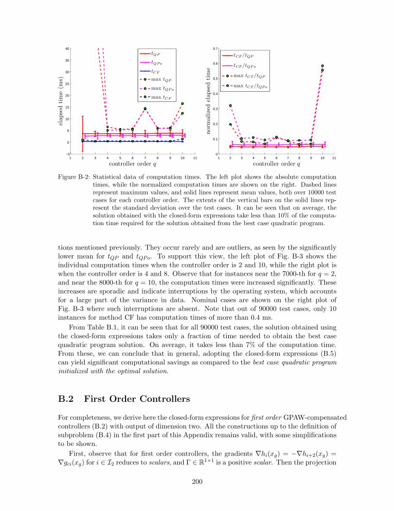
1 2 3 4 5 6 7 8 9 10 11−5

0

5

10

15

20

25

30

35

40

controller order q

elapsedtime(m

s)

tQP

tQPo

tCF

max tQP

max tQP o

max tCF

1 2 3 4 5 6 7 8 9 10 110

0.1

0.2

0.3

0.4

0.5

0.6

0.7

controller order q

norm

alizedelapsedtime

tCF /tQP

tCF /tQP o

max tCF /tQP

max tCF /tQPo

Figure B-2: Statistical data of computation times. The left plot shows the absolute computationtimes, while the normalized computation times are shown on the right. Dashed linesrepresent maximum values, and solid lines represent mean values, both over 10000 testcases for each controller order. The extents of the vertical bars on the solid lines rep-resent the standard deviation over the test cases. It can be seen that on average, thesolution obtained with the closed-form expressions take less than 10% of the computa-tion time required for the solution obtained from the best case quadratic program.

tions mentioned previously. They occur rarely and are outliers, as seen by the significantlylower mean for tQP and tQPo. To support this view, the left plot of Fig. B-3 shows theindividual computation times when the controller order is 2 and 10, while the right plot iswhen the controller order is 4 and 8. Observe that for instances near the 7000-th for q = 2,and near the 8000-th for q = 10, the computation times were increased significantly. Theseincreases are sporadic and indicate interruptions by the operating system, which accountsfor a large part of the variance in data. Nominal cases are shown on the right plot ofFig. B-3 where such interruptions are absent. Note that out of 90000 test cases, only 10instances for method CF has computation times of more than 0.4 ms.

From Table B.1, it can be seen that for all 90000 test cases, the solution obtained usingthe closed-form expressions takes only a fraction of time needed to obtain the best casequadratic program solution. On average, it takes less than 7% of the computation time.From these, we can conclude that in general, adopting the closed-form expressions (B.5)can yield significant computational savings as compared to the best case quadratic programinitialized with the optimal solution.

B.2 First Order Controllers

For completeness, we derive here the closed-form expressions for first order GPAW-compensatedcontrollers (B.2) with output of dimension two. All the constructions up to the definition ofsubproblem (B.4) in the first part of this Appendix remains valid, with some simplificationsto be shown.

First, observe that for first order controllers, the gradients ∇hi(xg) = −∇hi+2(xg) =∇gci(xg) for i ∈ I2 reduces to scalars, and Γ ∈ R1×1 is a positive scalar. Then the projection

200

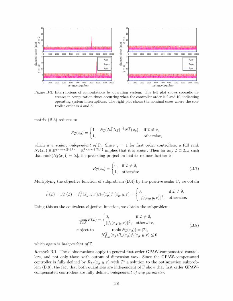
0 1000 2000 3000 4000 5000 6000 7000 8000 9000 100000

5

10

15

20

elap

sedtime(m

s) q=

2

0 1000 2000 3000 4000 5000 6000 7000 8000 9000 100000

5

10

15

20

instance number

q=

10

tQP

tQPo

tCF

0 1000 2000 3000 4000 5000 6000 7000 8000 9000 100000

5

10

15

20

elap

sedtime(m

s) q=

4

0 1000 2000 3000 4000 5000 6000 7000 8000 9000 100000

5

10

15

20

instance number

q=

8

tQP

tQPo

tCF

Figure B-3: Interruptions of computations by operating system. The left plot shows sporadic in-creases in computation times occurring when the controller order is 2 and 10, indicatingoperating system interruptions. The right plot shows the nominal cases where the con-troller order is 4 and 8.

matrix (B.3) reduces to

RI(xg) =

1−NI(NT

I NI)−1NT

I (xg), if I 6= ∅,1, otherwise,

which is a scalar, independent of Γ. Since q = 1 for first order controllers, a full rankNI(xg) ∈ Rq×max|I|,1 = R1×max|I|,1 implies that it is scalar. Then for any I ⊂ Isat suchthat rank(NI(xg)) = |I|, the preceding projection matrix reduces further to

RI(xg) =

0, if I 6= ∅,1, otherwise.

(B.7)

Multiplying the objective function of subproblem (B.4) by the positive scalar Γ, we obtain

F (I) = ΓF (I) = fTc (xg, y, r)RI(xg)fc(xg, y, r) =

0, if I 6= ∅,‖fc(xg, y, r)‖2, otherwise.

Using this as the equivalent objective function, we obtain the subproblem

maxI∈J

F (I) =

0, if I 6= ∅,‖fc(xg, y, r)‖2, otherwise,

subject to rank(NI(xg)) = |I|,NTIsat(xg)RI(xg)fc(xg, y, r) ≤ 0,

(B.8)

which again is independent of Γ.

Remark B.1. These observations apply to general first order GPAW-compensated control-lers, and not only those with output of dimension two. Since the GPAW-compensatedcontroller is fully defined by RI∗(xg, y, r) with I∗ a solution to the optimization subprob-lem (B.8), the fact that both quantities are independent of Γ show that first order GPAW-compensated controllers are fully defined independent of any parameter.

201

This is due to the fact that the GPAW parameter Γ only changes the way the controllerstate is modified on the boundary of the unsaturated region K. For first order controllers,there can only be two boundary points (in contrast to a higher dimensional surface) forwhich there is only one way to maintain controller state-output consistency, i.e. stop thescalar state evolution when the nominal update will cause constraint violations.

It is clear from subproblem (B.8) (as well as Proposition 2.5.2) that the optimal solutionis I∗ = ∅ whenever it is feasible. Recognizing that the rank condition always hold for I = ∅,it is feasible when condition A0 in (B.5) holds. For all other cases, we have RI∗(xg) = 0due to (B.7). Hence the closed-form expressions for the first order GPAW-compensatedcontroller with output of dimension two is given by

xg =

fc(xg, y, r), if A0,

0, otherwise,

ug = gc(xg), xg(0) = xc0,

where the switching condition A0 is identical to that in (B.5), reproduced here for ease ofreference

A0 ⇔ (gc1 < umax,1 ∨∇Tgc1fc ≤ 0) ∧ (gc1 > umin,1 ∨∇Tgc1fc ≥ 0)

∧ (gc2 < umax,2 ∨∇Tgc2fc ≤ 0) ∧ (gc2 > umin,2 ∨∇Tgc2fc ≥ 0).

202

Appendix C

Procedure to Apply GPAWCompensation

There are three different but equivalent ways (detailed in Sections 2.5 and 4.1) to realizegeneral GPAW-compensated controllers, while closed-form expressions (detailed in Appen-dices A and B) are available when the GPAW-compensated controller (or nominal controller)has output of dimension one or two. For ease of reference, we summarize the procedure toapply GPAW compensation here.

Step I If the nominal controller is of the form (2.24),

xc = fc(xc, y, r), xc(0) = xc0,

uc = gc(xc, y, r),(2.24)

i.e. with output function gc depending on measurement y and/or external refer-ence signal r, obtain an approximating controller of the form (2.26),

xc = fc(xc, y, r), xc(0) = xc0,

uc = gc(xc),(2.26)

with output function gc depending only on the controller state xc. One wayto approximate the nominal controller is discussed in Section 2.6, examples ofwhich are available in Sections 2.8.1, 6.1.2, 6.2.3, and A.2 (in Appendix A).

Step II Determine the GPAW parameter Γ. Note that any meaningful nominal controllerof the form (2.26) (possibly approximated due to Step I above) must be dynamic,i.e. with controller state of dimension at least one. When the nominal controlleris first order, this step can be bypassed (see Remark B.1). Theorems 4.4.3and 5.2.1 yield a Γ when they are applicable. When they are not applicable,some trial and error may be needed to determine Γ. Once Γ is determined, theGPAW-compensated controller is fully defined.

Step III Implement the GPAW-compensated controller.

(i) For GPAW-compensated controllers with output of dimension one or two,the closed-form expressions (A.5) and (B.5) are recommended for computa-tional efficiency (see Section B.1 in Appendix B). See Appendices A and Bfor specializations and possible simplifications.

203

(ii) For GPAW-compensated controllers with output of dimension greater thantwo, they can be implemented in one of three possible ways, namely:

(a) the combinatorial optimization formulation detailed in Section 2.5.The GPAW-compensated controller is defined by (2.27), (2.28), (2.29),(2.30), and the online solution to the combinatorial optimization sub-problem (2.31). Proposition 2.5.1 ensures the existence of solutions tosubproblem (2.31), which can always be found by an exhaustive searchalgorithm (see Remark 2.8);

(b) the quadratic program formulation detailed in Section 4.1. The GPAW-compensated controller is defined by (4.11), a matrix Φ obtained froma decomposition of the GPAW parameter Γ = ΦΦT, and the onlinesolution1 to the convex quadratic program (4.12);

(c) the projection onto a convex polyhedral cone formulation detailed inSection 4.1. This is identical to case (b), except that the quadratic pro-gram (4.12) is solved instead as a projection of the vector Φ−1fc(xg, y, r)onto the convex polyhedral cone K (4.10). For algorithms to projectonto convex polyhedral cones, see [170–175] and the references therein.

Step IV Determine controller state initialization. As shown in Section 6.1, an appropriatecontroller state initialization may yield significant improvements in the transientresponse of the GPAW-compensated system when the default choice xg(0) =xc(0), i.e. taking the initial state of the nominal controller, is “too far” from theunsaturated region. An example was shown in Section 6.1.3 on how to determinea reasonable state to initialize the GPAW-compensated controller.

The preceding summarizes the procedure to apply GPAW compensation to a generalsaturated nonlinear plant (1.1) driven by a nonlinear controller (1.3).

1See http://www.numerical.rl.ac.uk/qp/qp.html for a list of available quadratic program solvers.

204

Bibliography

[1] D. S. Bernstein and A. N. Michel, “A chronological bibliography on saturating actu-ators,” Int. J. Robust Nonlinear Control, vol. 5, no. 5, pp. 375 – 380, 1995.

[2] D. Liu and A. N. Michel, Dynamical Systems with Saturation Nonlinearities: Analysisand Design, ser. Lect. Notes Control Inf. Sci. London, Great Britain: Springer, 1994,vol. 195.

[3] T. Hu and Z. Lin, Control Systems with Actuator Saturation: Analysis and Design,ser. Control Eng. Boston, MA: Birkhauser, 2001.

[4] V. Kapila and K. M. Grigoriadis, Eds., Actuator Saturation Control, ser. Control Eng.New York, NY: Marcel Dekker, 2002.

[5] A. H. Glattfelder and W. Schaufelberger, Control Systems with Input and OutputConstraints, ser. Adv. Textb. Control Signal Process. London, United Kingdom:Springer, 2003.

[6] G. C. Goodwin, M. M. Seron, and J. A. De Dona, Constrained Control and Estimation:An Optimization Approach, ser. Commun. Control Eng. London, United Kingdom:Springer, 2005.

[7] P. Hippe, Windup in Control: Its Effects and Their Prevention, ser. Adv. Ind. Control.London, United Kingdom: Springer, 2006.

[8] S. Tarbouriech, G. Garcia, and A. H. Glattfelder, Eds., Advanced Strategies in ControlSystems with Input and Output Constraints, ser. Lect. Notes Control Inf. Sci. Berlin,Germany: Springer, 2007, vol. 346.

[9] Special Issue on Saturating Actuators, Int. J. Robust Nonlinear Control, vol. 5, no. 5,pp. 375 – 540, 1995.

[10] Special Issue on Control Problems with Constraints, Int. J. Robust Nonlinear Control,vol. 9, no. 10, pp. 583 – 734, Aug. 1999.

[11] Special Issue on Anti-windup, Int. J. Syst. Sci., vol. 37, no. 2, pp. 65 – 139, Feb. 2006.

[12] M. V. Kothare, P. J. Campo, M. Morari, and C. N. Nett, “A unified framework forthe study of anti-windup designs,” Automatica, vol. 30, no. 12, pp. 1869 – 1883, Dec.1994.

[13] C. Edwards and I. Postlethwaite, “Anti-windup and bumpless-transfer schemes,” Au-tomatica, vol. 34, no. 2, pp. 199 – 210, Feb. 1998.

205

[14] S. Tarbouriech and M. Turner, “Anti-windup design: an overview of some recentadvances and open problems,” IET Control Theory Appl., vol. 3, no. 1, pp. 1 – 19,Jan. 2009.

[15] J. C. Doyle, R. S. Smith, and D. F. Enns, “Control of plants with input saturationnonlinearities,” in Proc. American Control Conf., Minneapolis, MN, Jun. 1987, pp.1034 – 1039.

[16] D. A. Richardson, “Means for preventing reset wind-up in electronic controlapparatus,” U.S. Patent 3 197 711, Jul. 27, 1965. [Online]. Available: http://www.google.com/patents?id=JOFJAAAAEBAJ

[17] A. Visioli, Practical PID Control, ser. Adv. Ind. Control. London, United Kingdom:Springer, 2006.

[18] K. S. Walgama, S. Ronnback, and J. Sternby, “Generalisation of conditioning tech-nique for anti-windup compensators,” IEE Proc.-Control Theory Appl., vol. 139, no. 2,pp. 109 – 118, Mar. 1992.

[19] M. A. Dornheim, “Report pinpoints factors leading to YF-22 crash,” Aviat. WeekSpace Technol., vol. 137, no. 19, pp. 53 – 54, Nov. 1992.

[20] P. Butterworth-Hayes, “Gripen crash raises canard fears,” Aerosp. Am., vol. 32, no. 2,pp. 10 – 11, Feb. 1994.

[21] G. Stein, “Respect the unstable,” IEEE Control Syst. Mag., vol. 23, no. 4, pp. 12 –25, Aug. 2003.

[22] J. C. Lozier, “A steady state approach to the theory of saturable servo systems,” IRETrans. Autom. Control, vol. 1, no. 1, pp. 19 – 39, May 1956.

[23] E. Gilbert and I. Kolmanovsky, “Nonlinear tracking control in the presence of stateand control constraints: a generalized reference governor,” Automatica, vol. 38, no. 12,pp. 2063 – 2073, Dec. 2002.

[24] F. Morabito, A. R. Teel, and L. Zaccarian, “Nonlinear antiwindup applied to Euler-Lagrange systems,” IEEE Trans. Robot. Autom., vol. 20, no. 3, pp. 526 – 537, Jun.2004.

[25] A. E. Bryson, Jr. and Y.-C. Ho, Applied Optimal Control: Optimization, Estimation,and Control. Levittown, PA: Taylor & Francis, 1975.

[26] J. Sofrony, M. C. Turner, I. Postlethwaite, O. Brieger, and D. Leiβling, “Anti-windupsynthesis for PIO avoidance in an experimental aircraft,” in Proc. 45th IEEE Conf.Decision and Control, San Diego, CA, Dec. 2006, pp. 5412 – 5417.

[27] E. F. Mulder, P. Y. Tiwari, and M. V. Kothare, “Simultaneous linear and anti-windupcontroller synthesis using multiobjective convex optimization,” Automatica, vol. 45,no. 3, pp. 805 – 811, Mar. 2009.

[28] C. Burgat and S. Tarbouriech, “Intelligent anti-windup for systems with input mag-nitude saturation,” Int. J. Robust Nonlinear Control, vol. 8, no. 12, pp. 1085 – 1100,Oct. 1998.

206

[29] T. Kiyama and T. Iwasaki, “On the use of multi-loop circle criterion for saturatingcontrol synthesis,” Syst. Control Lett., vol. 41, no. 2, pp. 105 – 114, Oct. 2000.

[30] F. Wu, K. M. Grigoriadis, and A. Packard, “Anti-windup controller design using linearparameter-varying control methods,” Int. J. Control, vol. 73, no. 12, pp. 1104 – 1114,Aug. 2000.

[31] T. Kiyama, S. Hara, and T. Iwasaki, “Effectiveness and limitation of circle criterionfor lti robust control systems with control input nonlinearities of sector type,” Int. J.Robust Nonlinear Control, vol. 15, no. 17, pp. 873 – 901, Nov. 2005.

[32] J. M. Gomes da Silvar Jr., D. Limon, T. Alamo, and E. F. Camacho, “Output feedbackfor discrete-time systems with amplitude and rate constrained actuators,” in AdvancedStrategies in Control Systems with Input and Output Constraints, ser. Lect. NotesControl Inf. Sci., S. Tarbouriech, G. Garcia, and A. H. Glattfelder, Eds. Berlin,Germany: Springer, 2007, vol. 346, pp. 369 – 396.

[33] L. A. Zadeh and C. A. Desoer, Linear System Theory: The State Space Approach.Mineola, NY: Dover, 1991.

[34] E. D. Sontag, “An algebraic approach to bounded controllability of linear systems,”Int. J. Control, vol. 39, no. 1, pp. 181 – 188, Jan. 1984.

[35] L. Vandenberghe and S. Boyd, “Semidefinite programming,” SIAM Rev., vol. 38,no. 1, pp. 49 – 95, Mar. 1996.

[36] S. Boyd, L. El Ghaoui, E. Feron, and V. Balakrishnan, Linear Matrix Inequalities inSystem and Control Theory, ser. SIAM Stud. Appl. Math. Philadelphia, PA: SIAM,1994, vol. 15. [Online]. Available: http://www.stanford.edu/∼boyd/lmibook/index.html

[37] H. K. Khalil, Nonlinear Systems, 3rd ed. Upper Saddle River, NJ: Prentice Hall,2002.

[38] J.-J. Slotine and W. Li, Applied Nonlinear Control. Upper Saddle River, NJ: PrenticeHall, 1991.

[39] S. Sastry, Nonlinear Systems: Analysis, Stability, and Control, ser. Interdiscip. Appl.Math. New York, NY: Springer, 1999, vol. 10.

[40] R. Ortega, A. Lorıa, P. J. Nicklasson, and H. Sira-Ramırez, Passivity-based Controlof Euler-Lagrange Systems, ser. Commun. Control Eng. London, Great Britain:Springer, 1998.

[41] A. van der Schaft, L2-Gain and Passivity Techniques in Nonlinear Control, 2nd ed.,ser. Commun. Control Eng. London, Great Britain: Springer, 2000.

[42] R. C. Nelson, Flight Stability and Automatic Control, 2nd ed., ser. Aerosp. Sci. Tech-nol. Boston, MA: McGraw-Hill, 1998.

[43] S. M. LaValle, Planning Algorithms. New York, NY: Cambridge University Press,2006. [Online]. Available: http://planning.cs.uiuc.edu

207

[44] A. Isidori, Nonlinear Control Systems, 3rd ed., ser. Commun. Control Eng. London,Great Britain: Springer, 1995.

[45] ——, Nonlinear Control Systems II, ser. Commun. Control Eng. London, GreatBritain: Springer, 1999.

[46] W. M. Haddad and V. Chellaboina, Nonlinear Dynamical Systems and Control: ALyapunov-based Approach. Princeton, NJ: Princeton University Press, 2008.

[47] T. Hu, A. N. Pitsillides, and Z. Lin, “Null controllability and stabilization of linearsystems subject to asymmetric actuator saturation,” in Actuator Saturation Control,ser. Control Eng., V. Kapila and K. M. Grigoriadis, Eds. New York, NY: MarcelDekker, 2002, ch. 3, pp. 47 – 76.

[48] B. G. Romanchuk and M. C. Smith, “Incremental gain analysis of linear systems withbounded controls and its application to the antiwindup problem,” in Proc. 35th IEEEConf. Decision and Control, vol. 3, Kobe, Japan, Dec. 1996, pp. 2942 – 2947.

[49] N. Kapoor, A. R. Teel, and P. Daoutidis, “An anti-windup design for linear systemswith input saturation,” Automatica, vol. 34, no. 5, pp. 559 – 574, May 1998.

[50] H. J. Sussmann, “Existence and uniqueness of minimal realizations of nonlinear sys-tems,” Math. Syst. Theory, vol. 10, no. 1, pp. 263 – 284, 1977.

[51] R. Hanus, M. Kinnaert, and J.-L. Henrotte, “Conditioning technique, a general anti-windup and bumpless transfer method,” Automatica, vol. 23, no. 6, pp. 729 – 739,Nov. 1987.

[52] R. Hanus and Y. Peng, “Conditioning technique for controllers with time delays,”IEEE Trans. Autom. Control, vol. 37, no. 5, pp. 689 – 692, May 1992.

[53] H. A. Fertik and C. W. Ross, “Direct digital control algorithm with anti-windupfeature,” ISA Trans., vol. 6, no. 4, pp. 317 – 328, 1967.

[54] J. E. Dennis, Jr. and R. B. Schnabel, Numerical Methods for Unconstrained Optimiza-tion and Nonlinear Equations, ser. Classics Appl. Math. Philadelphia, PA: SIAM,1996, vol. 16.

[55] J.-K. Park and C.-H. Choi, “Author’s reply,” IEEE Trans. Autom. Control, vol. 41,no. 10, pp. 1550 – 1551, Oct. 1996.

[56] J.-P. Calvet and Y. Arkun, “Feedforward and feedback linearization of nonlinearsystems and its implementation using internal model control (IMC),” Ind. Eng. Chem.Res., vol. 27, no. 10, pp. 1822 – 1831, Oct. 1988.

[57] T. A. Kendi and F. J. Doyle III, “An anti-windup scheme for multivariable nonlinearsystems,” J. Process Control, vol. 7, no. 5, pp. 329 – 343, Oct. 1997.

[58] F. J. Doyle III, “An anti-windup input-output linearization scheme for SISO systems,”J. Proc. Control, vol. 9, no. 3, pp. 213 – 220, Jun. 1999.

[59] N. Kapoor and P. Daoutidis, “An observer-based anti-windup scheme for non-linearsystems with input constraints,” Int. J. Control, vol. 72, no. 1, pp. 18 – 29, Jan. 1999.

208

[60] W. Wu, “Anti-windup schemes for a constrained continuous stirred tank reactor pro-cess,” Ind. Eng. Chem. Res., vol. 41, no. 7, pp. 1796 – 1804, 2002.

[61] G. Herrmann, M. C. Turner, P. Menon, D. G. Bates, and I. Postlethwaite, “Anti-windup synthesis for nonlinear dynamic inversion controllers,” in Proc. 5th IFACSymp. Robust Control Design, vol. 5, no. 1, Toulouse, France, Jul. 2006.

[62] P. P. Menon, G. Herrmann, M. C. Turner, D. G. Bates, and I. Postlethwaite, “Gen-eral anti-windup synthesis for input constrained nonlinear systems controlled usingnonlinear dynamic inversion,” in Proc. 45th IEEE Conf. Decision and Control, SanDiego, CA, Dec. 2006, pp. 5435 – 5440.

[63] P. P. Menon, G. Herrmann, M. C. Turner, M. Lowenberg, D. Bates, and I. Postleth-waite, “Dynamic wind tunnel rig implementation of nonlinear dynamic inversion basedanti-windup scheme,” in Proc. AIAA Guidance Navigation and Control Conf. and Ex-hibit, Honolulu, HI, Aug. 2008, AIAA–2008–7166.

[64] P. P. Menon, G. Herrmann, M. Turner, M. Lowenberg, D. Bates, and I. Postlethwaite,“Nonlinear dynamic inversion based anti-windup - an aerospace application,” in Proc.17th IFAC World Congress, vol. 17, no. 1, Seoul, Korea, Jul. 2008, pp. 14 156 – 14 161.

[65] S.-S. Yoon, J.-K. Park, and T.-W. Yoon, “Dynamic anti-windup scheme for feedbacklinearizable nonlinear control systems with saturating inputs,” Automatica, vol. 44,no. 12, pp. 3176 – 3180, Dec. 2008.

[66] G. Herrmann, P. P. Menon, M. C. Turner, D. G. Bates, and I. Postlethwaite, “Anti-windup synthesis for nonlinear dynamic inversion control schemes,” Int. J. RobustNonlinear Control, vol. 20, no. 13, pp. 1465 – 1482, Sep. 2010.

[67] C. I. Byrnes, “Remarks on nonlinear planar control systems which are linearizable byfeedback,” Syst. Control Lett., vol. 5, no. 6, pp. 363 – 367, May 1985.

[68] P. Rouchon, “Necessary condition and genericity of dynamic feedback linearization,”J. Math. Syst. Estimat. Control, vol. 4, no. 2, pp. 1 – 14, 1994.

[69] Q. Hu and G. P. Rangaiah, “Anti-windup schemes for uncertain nonlinear systems,”IET Control Theory Appl., vol. 147, no. 3, pp. 321 – 329, May 2000.

[70] E. N. Johnson and A. J. Calise, “Neural network adaptive control of systems withinput saturation,” in Proc. American Control Conf., Arlington, VA, Jun. 2001, pp.3527 – 3532.

[71] ——, “Limited authority adaptive flight control for reusable launch vehicles,” J. Guid.Control Dyn., vol. 26, no. 6, pp. 906 – 913, Nov. – Dec. 2003.

[72] H. M. Do, T. Basar, and J. Y. Choi, “An anti-windup design for single input adaptivecontrol systems in strict feedback form,” in Proc. American Control Conf., vol. 3,Boston, MA, Jun./Jul. 2004, pp. 2551 – 2556.

[73] M. Yokoyama, G.-N. Kim, and M. Tsuchiya, “Integral sliding mode control with anti-windup compensation and its application to a power assist system,” J. Vib. Control,vol. 16, no. 4, pp. 503 – 512, Apr. 2010.

209

[74] A. R. Teel and N. Kapoor, “The L2 anti-windup problem: Its definition and solution,”in Proc. European Control Conf., Brussels, Belgium, Jul. 1997.

[75] M. Soroush and S. Valluri, “Calculation of optimal feasible controller output in mul-tivariable processes with input constraints,” in Proc. American Control Conf., vol. 5,Albuquerque, NM, Jun. 1997, pp. 3475 – 3479.

[76] S. Valluri and M. Soroush, “Analytical control of SISO nonlinear processes with inputconstraints,” AIChE J., vol. 44, no. 1, pp. 116 – 130, Jan. 1998.

[77] M. Soroush and S. Valluri, “Optimal directionality compensation in processes withinput saturation non-linearities,” Int. J. Control, vol. 72, no. 17, pp. 1555 – 1564,Nov. 1999.

[78] M. Soroush and N. Mehranbod, “Optimal compensation for directionality in processeswith a saturating actuator,” Comput. Chem. Eng., vol. 26, no. 11, pp. 1633 – 1641,Nov. 2002.

[79] M. Soroush and P. Daoutidis, “Optimal windup and directionality compensation ininput-constrained nonlinear systems,” in Actuator Saturation Control, ser. ControlEng., V. Kapila and K. M. Grigoriadis, Eds. New York, NY: Marcel Dekker, 2002,ch. 9, pp. 227 – 246.

[80] S. Valluri and M. Soroush, “A non-linear controller design method for processes withsaturating actuators,” Int. J. Control, vol. 76, no. 7, pp. 698 – 716, Jan. 2003.

[81] M. Soroush, S. Valluri, and N. Mehranbod, “Nonlinear control of input-constrainedsystems,” Comput. Chem. Eng., vol. 30, no. 1, pp. 158 – 181, Nov. 2005.

[82] D. Q. Mayne, J. B. Rawlings, C. V. Rao, and P. O. M. Scokaert, “Constrained modelpredictive control: Stability and optimality,” Automatica, vol. 36, no. 6, pp. 789 –814, Jun. 2000.

[83] P. Kapasouris, M. Athans, and G. Stein, “Design of feedback control systems for stableplants with saturating actuators,” in Proc. 27th IEEE Conf. Decision and Control,vol. 1, Austin, TX, Dec. 1988, pp. 469 – 479.

[84] E. G. Gilbert and K. T. Tan, “Linear systems with state and control constraints:The theory and application of maximal output admissible sets,” IEEE Trans. Autom.Control, vol. 36, no. 9, pp. 1008 – 1020, Sep. 1991.

[85] A. Bemporad and E. Mosca, “Constraint fulfilment in feedback control via predic-tive reference management,” in Proc. 3rd IEEE Conf. Control Applications, vol. 3,Glasgow, Scotland, Aug. 1994, pp. 1909 – 1914.

[86] ——, “Constraint fulfilment in control systems via predictive reference management,”in Proc. 33th IEEE Conf. Decision and Control, vol. 3, Lake Buena Vista, FL, Dec.1994, pp. 3017 – 3022.

[87] E. G. Gilbert, I. Kolmanovsky, and K. T. Tan, “Nonlinear control of discrete-timelinear systems with state and control constraints: A reference governor with globalconvergence properties,” in Proc. 33rd IEEE Conf. Decision and Control, vol. 1, LakeBuena Vista, FL, Dec. 1994, pp. 144 – 149.

210

[88] A. Bemporad and E. Mosca, “Nonlinear predictive reference governor for constrainedcontrol systems,” in Proc. 34th IEEE Conf. Decision and Control, vol. 2, New Orleans,LA, Dec. 1995, pp. 1205 – 1210.

[89] E. G. Gilbert and I. Kolmanovsky, “Discrete-time reference governors for systemswith state and control constraints and disturbance inputs,” in Proc. 34th IEEE Conf.Decision and Control, vol. 2, New Orleands, LA, Dec. 1995, pp. 1189 – 1194.

[90] E. G. Gilbert, I. Kolmanovsky, and K. T. Tan, “Discrete-time reference governors andthe nonlinear control of systems with state and control constrains,” Int. J. RobustNonlinear Control, vol. 5, no. 5, pp. 487 – 504, 1995.

[91] A. Casavola and E. Mosca, “Reference governor for constrained uncertain linear sys-tems subject to bounded input disturbances,” in Proc. 35th IEEE Conf. Decision andControl, vol. 3, Koba, Japan, Dec. 1996, pp. 3531 – 3536.

[92] A. Bemporad, A. Casavola, and E. Mosca, “Nonlinear control of constrained linearsystems via predictive reference management,” IEEE Trans. Autom. Control, vol. 42,no. 3, pp. 340 – 349, Mar. 1997.

[93] E. G. Gilbert and I. Kolmanovsky, “Fast reference governors for systems with stateand control constraints and disturbance inputs,” Int. J. Robust Nonlinear Control,vol. 9, no. 15, pp. 1117 – 1141, Dec. 1999.

[94] K. Kogiso and K. Hirata, “Reference governor for constrained systems with time-varying references,” Robot. Auton. Syst., vol. 57, no. 3, pp. 289 – 295, Mar. 2009.

[95] A. Bemporad, “Reference governor for constrained nonlinear systems,” IEEE Trans.Autom. Control, vol. 43, no. 3, pp. 415 – 419, Mar. 1998.

[96] D. Angeli and E. Mosca, “Command governors for constrained nonlinear systems,”IEEE Trans. Autom. Control, vol. 44, no. 4, pp. 816 – 820, Apr. 1999.

[97] E. G. Gilbert and I. V. Kolmanovsky, “Set-point control of nonlinear systems withstate and control constraints: A Lyapunov-function, reference-governor approach,” inProc. 38th IEEE Conf. Decision and Control, vol. 3, Phoenix, AZ, Dec. 1999, pp.2507 – 2512.

[98] R. H. Miller, I. Komanovsky, E. G. Gilbert, and P. D. Washabaugh, “Control ofconstrained nonlinear systems: A case study,” IEEE Control Syst. Mag., vol. 20,no. 1, pp. 23 – 32, Feb. 2000.

[99] T. Hatanaka and K. Takaba, “Output feedback reference governor for nonlinear sys-tems,” in Proc. 44th IEEE Conf. Decision and Control & European Control Conf.,Seville, Spain, Dec. 2005, pp. 7558 – 7563.

[100] J. B. Rosen, “The gradient projection method for nonlinear programming. part I.linear constraints,” J. Soc. Ind. Appl. Math., vol. 8, no. 1, pp. 181 – 217, Mar. 1960.

[101] ——, “The gradient projection method for nonlinear programming. part II. nonlinearconstraints,” J. Soc. Ind. Appl. Math., vol. 9, no. 4, pp. 514 – 532, Dec. 1961.

211

[102] J.-J. E. Slotine and J. A. Coetsee, “Adaptive sliding controller synthesis for non-linearsystems,” Int. J. Control, vol. 43, no. 6, pp. 1631 – 1651, Jun. 1986.

[103] L. Hou and A. N. Michel, “Asymptotic stability of systems with saturation con-straints,” IEEE Trans. Autom. Control, vol. 43, no. 8, pp. 1148 – 1154, Aug. 1998.

[104] H. Fang and Z. Lin, “Stability analysis for linear systems under state constraints,”IEEE Trans. Autom. Control, vol. 49, no. 6, pp. 950 – 955, Jun. 2004.

[105] X. Ji, T. Liu, and M. Ren, “Stability analysis for continuous-time planar linear sys-tems with state saturation,” in Proc. Chinese Conf. Decision and Control, Shandong,China, Jul. 2008, pp. 4355 – 4359.

[106] W. Guan and G. H. Yang, “Analysis and design of output feedback control systemsin the presence of state saturation,” in Proc. American Control Conf., St. Louis, MO,Jun. 2009, pp. 5677 – 5682.

[107] P. Dupuis and A. Nagurney, “Dynamical systems and variational inequalities,” Ann.Oper. Res., vol. 44, no. 1, pp. 7 – 42, Feb. 1993.

[108] D. Zhang and A. Nagurney, “On the stability of projected dynamical systems,” J.Optim. Theory Appl., vol. 85, no. 1, pp. 97 – 124, Apr. 1995.

[109] A. Nagurney and D. Zhang, Projected Dynamical Systems and Variational Inequalitieswith Applications, ser. Int. Ser. Oper. Res. Manag. Sci. Norwell, MA: Kluwer, 1996.

[110] M.-G. Cojocaru and L. B. Jonker, “Existence of solutions to projected differentialequations in Hilbert spaces,” Proc. Amer. Math. Soc., vol. 132, no. 1, pp. 183 – 193,Jan. 2004.

[111] D. G. Eksten and G. F. Ohlson, “Automatic control circuit utilizing input andinternal signals controlling reset for providing improved step response,” U.S. Patent3 219 936, Nov. 23, 1965. [Online]. Available: http://www.google.com/patents?id=AQdnAAAAEBAJ

[112] J. O. Jacques, “Input for digital controller,” U.S. Patent 3 387 282, Jun. 4, 1968.[Online]. Available: http://www.google.com/patents?id=0yVnAAAAEBAJ

[113] J. O. Jacques, D. Montgomery, and P. A. Kuckein, “Digital controller with automaticbalance and manually adjusted operating point,” U.S. Patent 3 479 493, Nov. 18,1969. [Online]. Available: http://www.google.com/patents?id=1a1vAAAAEBAJ

[114] J. O. Jacques, “Digital control system with integral clamping,” U.S. Patent3 495 074, Feb. 10, 1970. [Online]. Available: http://www.google.com/patents?id=l7JZAAAAEBAJ

[115] J. O. Jacques, P. A. Kuckein, and R. K. Oswald, “Closed loop controller havingdigital integrator with variable gain,” U.S. Patent 3 513 302, May 19, 1970. [Online].Available: http://www.google.com/patents?id=0Pd0AAAAEBAJ

[116] J. W. Slover, “Leak preventing control for heat exchangers,” U.S. Patent3 400 753, Sep. 10, 1968. [Online]. Available: http://www.google.com/patents?id=Yg9jAAAAEBAJ

212

[117] F. B. Davis III and C. W. Ross, “Load-frequency control system withoutproportional windup,” U.S. Patent 3 525 857, Aug. 25, 1970. [Online]. Available:http://www.google.com/patents?id=zYd1AAAAEBAJ

[118] G. Labinaz, M. M. Bayoumi, and K. Rudie, “A survey of modeling and control ofhybrid systems,” Annu. Rev. Control, vol. 21, pp. 79 – 92, 1997.

[119] H. Lin and P. J. Antsaklis, “Stability and stabilization of switched linear systems: Asurvey of recent results,” IEEE Trans. Autom. Control, vol. 54, no. 2, pp. 308 – 322,Feb. 2009.

[120] A. F. Filippov, Differential Equations with Discontinuous Righthand Sides, ser. Math.Appl. Dordrecht, Netherlands: Kluwer Academic Publishers, 1988.

[121] D. P. Bertsekas, Nonlinear Programming, 2nd ed., ser. Optim. Comput. Belmont,MA: Athena Scientific, 1999.

[122] P. A. Ioannou and J. Sun, Robust Adaptive Control. Upper Saddle River,NJ: Prentice Hall, 1996. [Online]. Available: http://www-rcf.usc.edu/∼ioannou/Robust Adaptive Control.htm

[123] J.-B. Pomet and L. Praly, “Adaptive nonlinear regulation: Estimation from the Lya-punov equation,” IEEE Trans. Autom. Control, vol. 37, no. 6, pp. 729 – 740, Jun.1992.

[124] R. A. Horn and C. R. Johnson, Matrix Analysis. New York, NY: Cambridge Uni-versity Press, 1985.

[125] G. A. Korn and T. M. Korn, Mathematical Handbook for Scientists and Engineers:Definitions, Theorems, and Formulas for Reference and Review. Mineola, NY: Dover,1968.

[126] J. Dattorro, Convex Optimization & Euclidean Distance Geometry. Palo Alto,CA: Meboo, 2005, version 2010.06.04. [Online]. Available: http://meboo.convexoptimization.com/Meboo.html

[127] J. Teo and J. P. How, “Anti-windup compensation for nonlinear systems via gradientprojection: Application to adaptive control,” in Proc. 48th IEEE Conf. Decision andControl & 28th Chinese Control Conf., Shanghai, China, Dec. 2009, pp. 6910 – 6916.

[128] G. Grimm, J. Hatfield, I. Postlethwaite, A. R. Teel, M. C. Turner, and L. Zaccarian,“Antiwindup for stable linear systems with input saturation: An LMI-based synthe-sis,” IEEE Trans. Autom. Control, vol. 48, no. 9, pp. 1509 – 1525, Sep. 2003.

[129] B. Brogliato, R. Lozano, B. Maschke, and O. Egeland, Dissipative Systems Analysisand Control: Theory and Applications, 2nd ed., ser. Commun. Control Eng. London,United Kingdom: Springer, 2007.

[130] J. A. De Dona, G. C. Goodwin, and M. M. Seron, “Anti-windup and model predictivecontrol: Reflections and connections,” Eur. J. Control, vol. 6, no. 5, pp. 467 – 477,2000.

213

[131] L. Lu and Z. Lin, “A switching anti-windup design using multiple Lyapunov func-tions,” IEEE Trans. Autom. Control, vol. 55, no. 1, pp. 142 – 148, Jan. 2010.

[132] R. J. Mantz and H. De Battista, “Sliding mode compensation for windup and directionof control problems in two-input-two-output proportional-integral controllers,” Ind.Eng. Chem. Res., vol. 41, no. 13, pp. 3179 – 3185, 2002.

[133] R. J. Mantz, H. De Battista, and F. D. Bianchi, “Sliding mode conditioning forconstrained processes,” Ind. Eng. Chem. Res., vol. 43, no. 26, pp. 8251 – 8256, 2004.

[134] F. Garelli, R. J. Mantz, and H. De Battista, “Collective sliding-mode technique formultivariable bumpless transfer,” Ind. Eng. Chem. Res., vol. 41, no. 8, pp. 2721 –2727, 2008.

[135] J. K. Hale, Ordinary Differential Equations, 2nd ed. Mineola, NY: Dover, 1997.

[136] A. A. Andronov, A. A. Vitt, and S. E. Khaikin, Theory of Oscillators, ser. Int. Ser.Monogr. Phys. Oxford, England: Pergamon Press, 1966, vol. 4.

[137] M. Vidyasagar, Nonlinear Systems Analysis, 2nd ed. Englewood Cliffs, NJ: PrenticeHall, 1993.

[138] E. A. Coddington and N. Levinson, Theory of Ordinary Differential Equations, ser.Int. Ser. Pure Appl. Math. New York, NY: McGraw-Hill, 1955.

[139] O. Hajek, Control Theory in the Plane, 2nd ed., ser. Lect. Notes Control Inf. Sci.Berlin, Germany: Springer, 2009, vol. 153.

[140] R. Mantri, A. Saberi, and V. Venkatasubramanian, “Stability analysis of continuoustime planar systems with state saturation nonlinearity,” IEEE Trans. Circuits Syst.I, vol. 45, no. 9, pp. 989 – 993, Sep. 1998.

[141] J. Alvarez, R. Suarez, and J. Alvarez, “Planar linear systems with single saturatedfeedback,” Syst. Control Lett., vol. 20, no. 4, pp. 319 – 326, Apr. 1993.

[142] J.-Y. Favez, P. Mullhaupt, B. Srinivasan, and D. Bonvin, “Attraction region of planarlinear systems with one unstable pole and saturated feedback,” J. Dyn. Control Syst.,vol. 12, no. 3, pp. 331 – 355, Jul. 2006.

[143] T. Hu, L. Qiu, and Z. Lin, “Stabilization of LTI systems with planar anti-stabledynamics using saturated linear feedback,” in Proc. 37th IEEE Conf. Decision andControl, Tampa, FL, Dec. 1998, pp. 389 – 394.

[144] T. Hu, Z. Lin, and L. Qiu, “Stabilization of exponentially unstable linear systemswith saturating actuators,” IEEE Trans. Autom. Control, vol. 46, no. 6, pp. 973 –979, Jun. 2001.

[145] M. L. Corradini, A. Cristofaro, and F. Giannoni, “Sharp estimates on the region ofattraction of planar linear systems with bounded controls,” in Proc. 48th IEEE Conf.Decision and Control & 28th Chinese Control Conf., Shanghai, China, Dec. 2009, pp.5345 – 5350.

214

[146] F. Liu, G. T.-C. Chiu, E. S. Hamby, and Y. Eun, “Time maximum control for a classof single-input planar affine control systems and constraints,” in Proc. 48th IEEEConf. Decision and Control & 28th Chinese Control Conf., Shanghai, China, Dec.2009, pp. 5045 – 5050.

[147] J. A. Ball, M. V. Day, and P. Kachroo, “Robust feedback control of a single serverqueueing system,” Math. Control Signal Syst., vol. 12, no. 4, pp. 307 – 345, Nov. 1999.

[148] J. A. Ball, M. V. Day, T. Yu, and P. Kachroo, “Robust L2-gain control for nonlinearsystems with projection dynamics and input constraints: an example from trafficcontrol,” Automatica, vol. 35, no. 3, pp. 429 – 444, Mar. 1999.

[149] K. Kuhnen and P. Krejci, “Identification of linear error-models with projected dy-namical systems,” Math. Comput. Model. Dyn. Syst., vol. 10, no. 1, pp. 59 – 91, Mar.2004.

[150] K. Kuhnen and P. Krejcı, “An adaptive gradient law with projection for non-smoothconvex boundaries,” Eur. J. Control, vol. 12, no. 6, pp. 606 – 619, 2006.

[151] B. Brogliato, A. Daniilidis, C. Lemarechal, and V. Acary, “On the equivalence betweencomplementarity systems, projected systems and differential inclusions,” Syst. ControlLett., vol. 55, no. 1, pp. 45 – 51, Jan. 2006.

[152] A. van der Schaft and H. Schumacher, An Introduction to Hybrid Dynamical Systems,ser. Lect. Notes Control Inf. Sci. London, Great Britain: Springer, 2000, vol. 251.

[153] S. Skogestad and I. Postlethwaite, Multivariable Feedback Control: Analysis and De-sign. West Sussex, England: Wiley, 1996.

[154] W. Rudin, Principles of Mathematical Analysis, 3rd ed., ser. Int. Ser. Pure Appl.Math. New York, NY: McGraw-Hill, 1976.

[155] J. P. LaSalle, “Some extensions of Liapunov’s second method,” IRE Trans. CircuitTheory, vol. 7, no. 4, pp. 520 – 527, Dec. 1960.

[156] S. Weissenberger, “Stability regions of large-scale systems,” Automatica, vol. 9, no. 6,pp. 653 – 663, Nov. 1973.

[157] R. Genesio, M. Tartaglia, and A. Vicino, “On the estimation of asymptotic stabilityregions: State of the art and new proposals,” IEEE Trans. Autom. Control, vol. 30,no. 8, pp. 747 – 755, Aug. 1985.

[158] J. Zaborszky, G. Huang, B. Zheng, and T.-C. Leung, “On the phase portrait of a classof large nonlinear dynamic systems such as the power system,” IEEE Trans. Autom.Control, vol. 33, no. 1, pp. 4 – 15, Jan. 1988.

[159] H.-D. Chiang, M. W. Hirsch, and F. F. Wu, “Stability regions of nonlinear autonomousdynamical systems,” IEEE Trans. Autom. Control, vol. 33, no. 1, pp. 16 – 27, Jan.1988.

[160] H.-D. Chiang and J. S. Thorp, “Stability regions of nonlinear dynamical systems: Aconstructive methodology,” IEEE Trans. Autom. Control, vol. 34, no. 12, pp. 1229 –1241, Dec. 1989.

215

[161] A. Levin, “An analytical method of estimating the domain of attraction for polynomialdifferential equations,” IEEE Trans. Autom. Control, vol. 39, no. 12, pp. 2471 – 2475,Dec. 1994.

[162] H.-D. Chiang and L. Fekih-Ahmed, “Quasi-stability regions of nonlinear dynamicalsystems: Optimal estimations,” IEEE Trans. Circuits Syst. I, vol. 43, no. 8, pp. 636– 643, Aug. 1996.

[163] L. Gruyitch, J.-P. Richard, P. Borne, and J.-C. Gentina, Stability Domains, ser. Non-linear Syst. Aviat. Aerosp. Aeronaut. Astronaut. Boca Raton, FL: Chapman & Hall,2004, vol. 1.

[164] W. Tan and A. Packard, “Stability region analysis using polynomial and compos-ite polynomial Lyapunov functions and sum-of-squares programming,” IEEE Trans.Autom. Control, vol. 53, no. 2, pp. 565 – 571, Mar. 2008.

[165] G. Chesi, “Estimating the domain of attraction for non-polynomial systems via LMIoptimizations,” Automatica, vol. 45, no. 6, pp. 1536 – 1541, Jun. 2009.

[166] A. I. Zecevic and D. D. Siljak, “Estimating the region of attraction for large-scalesystems with uncertainties,” Automatica, vol. 46, no. 2, pp. 445 – 451, Feb. 2010.

[167] S. J. Russell and P. Norvig, Artificial Intelligence: A Modern Approach, 2nd ed., ser.Artif. Intell. Upper Saddle River, NJ: Prentice Hall, 2003.

[168] J. Guckenheimer and P. Holmes, Nonlinear Oscillations, Dynamical Systems, andBifurcations of Vector Fields, ser. Appl. Math. Sci. New York, NY: Springer, 2002,vol. 42.

[169] J. Stoer and C. Witzgall, Convexity and Optimization in Finite Dimensions I, ser.Die Grundlehren der mathematischen Wissenschaften. Berlin, Germany: Springer,1970, vol. 163.

[170] M. Tenenhaus, “Canonical analysis of two convex polyhedral cones and applications,”Psychometrika, vol. 53, no. 4, pp. 503 – 524, Dec. 1988.

[171] R. L. Dykstra, “An algorithm for restricted least squares regression,” J. Am. Stat.Assoc., vol. 78, no. 384, pp. 837 – 842, Dec. 1983.

[172] N. Gaffke and R. Mathar, “A cyclic projection algorithm via duality,” Metrika, vol. 36,no. 1, pp. 29 – 54, Dec. 1989.

[173] T. Hyunh, C. Lassez, and J.-L. Lassez, “Practical issues on the projection of polyhe-dral sets,” Ann. Math. Artif. Intell., vol. 6, no. 4, pp. 295 – 315, Dec. 1992.

[174] L. M. Bregman, Y. Censor, S. Reich, and Y. Zepkowitz-Malachi, “Finding the projec-tion of a point onto the intersection of convex sets via projections onto half-spaces,”J. Approx. Theory, vol. 124, no. 2, pp. 194 – 218, Oct. 2003.

[175] A. B. Nemeth and S. Z. Nemeth, “How to project onto an isotone projection cone,”Linear Alg. Appl., vol. 433, no. 1, pp. 41 – 51, Jul. 2010.

[176] S. Boyd and L. Vandenberghe, Convex Optimization. Cambridge, United Kingdom:Cambridge University Press, 2004.

216

[177] R. T. Rockafellar, Convex Analysis, ser. Princeton Landmarks Math. Princeton, NJ:Princeton University Press, 1970.

[178] F. A. Valentine, Convex Sets, ser. McGraw-Hill Ser. High. Math. New York, NY:McGraw-Hill, 1964.

[179] A. Baıllo and A. Cuevas, “On the estimation of a star-shaped set,” Adv. Appl. Probab.,vol. 33, no. 4, pp. 717 – 726, Dec. 2001.

[180] J.-B. Hiriart-Urruty and C. Lemarechal, Fundamentals of Convex Analysis, ser.Grundlehren Text Ed. Berlin, Germany: Springer, 2001.

[181] A. N. Michel, K. Wang, and B. Hu, Qualitative Theory of Dynamical Systems: TheRole of Stability Preserving Mappings, 2nd ed., ser. Pure Appl. Math. New York,NY: Marcel Dekker, 2001, vol. 239.

[182] D. Carlson, “Block diagonal semistability factors and Lyapunov semistability of blocktriangular matrices,” Linear Alg. Appl., vol. 172, pp. 1 – 25, Jul. 1992.

[183] G. Balas, R. Chiang, A. Packard, and M. Safonov, Robust Control ToolboxTM 3:User’s Guide, MathWorks, Natick, MA, 2010.

[184] F. Morabito, “Sintesi e validazione di tecniche di controllo anti-windup per sistemiEulero–Lagrange con saturazione sugli ingressi,” Master’s thesis, Univ. Rome “TorVergata”, Rome, Italy, 2002.

[185] P. R. Belanger, Control Engineering: A Modern Approach. Orlando, FL: SaundersCollege Publishing, 1995.

[186] Optimization ToolboxTM 5: User’s Guide, Mathworks, Natick, MA, 2010.

[187] K. J. Astrom and L. Rundqwist, “Integrator windup and how to avoid it,” in Proc.American Control Conf., Pittsburgh, PA, Jun. 1989, pp. 1693 – 1698.

[188] K. J. Astrom and T. Hagglund, PID Controllers: Theory, Design, and Tuning, 2nd ed.Research Triangle Park, NC: Instrument Society of America, 1995.

[189] A. O’Dwyer, Handbook of PI and PID Controller Tuning Rules, 2nd ed. London,United Kingdom: Imperial College Press, 2006.

[190] G. J. Silva, A. Datta, and S. P. Bhattacharyya, PID Controllers for Time-DelaySystems, ser. Control Eng. Boston, MA: Birkhauser, 2005.

[191] Q.-G. Wang, Z. Ye, W.-J. Cai, and C.-C. Hang, PID Control for Multivariable Pro-cesses, ser. Lect. Notes Control Inf. Sci. Berlin, Germany: Springer, 2008, vol. 373.

[192] Y. Choi and W. K. Chung, PID Trajectory Tracking Control for Mechanical Systems,ser. Lect. Notes Control Inf. Sci. Berlin, Germany: Springer, 2004, vol. 298.

217