Gradient Episodic Memory for Continual Learning

David Lopez-Paz and Marc’Aurelio RanzatoFacebook Artificial Intelligence Research

{dlp,ranzato}@fb.com

Abstract

One major obstacle towards AI is the poor ability of models to solve new prob-lems quicker, and without forgetting previously acquired knowledge. To betterunderstand this issue, we study the problem of continual learning, where the modelobserves, once and one by one, examples concerning a sequence of tasks. First,we propose a set of metrics to evaluate models learning over a continuum of data.These metrics characterize models not only by their test accuracy, but also in termsof their ability to transfer knowledge across tasks. Second, we propose a modelfor continual learning, called Gradient Episodic Memory (GEM) that alleviatesforgetting, while allowing beneficial transfer of knowledge to previous tasks. Ourexperiments on variants of the MNIST and CIFAR-100 datasets demonstrate thestrong performance of GEM when compared to the state-of-the-art.

1 Introduction

The starting point in supervised learning is to collect a training set Dtr = {(xi, yi)}ni=1, whereeach example (xi, yi) is composed by a feature vector xi ∈ X , and a target vector yi ∈ Y . Mostsupervised learning methods assume that each example (xi, yi) is an identically and independentlydistributed (iid) sample from a fixed probability distribution P , which describes a single learning task.The goal of supervised learning is to construct a model f : X → Y , used to predict the target vectorsy associated to unseen feature vectors x, where (x, y) ∼ P . To accomplish this, supervised learningmethods often employ the Empirical Risk Minimization (ERM) principle [Vapnik, 1998], where fis found by minimizing 1

|Dtr|∑

(xi,yi)∈Dtr`(f(xi), yi), where ` : Y × Y → [0,∞) is a loss function

penalizing prediction errors. In practice, ERM often requires multiple passes over the training set.

ERM is a major simplification from what we deem as human learning. In stark contrast to learningmachines, learning humans observe data as an ordered sequence, seldom observe the same exampletwice, they can only memorize a few pieces of data, and the sequence of examples concerns differentlearning tasks. Therefore, the iid assumption, along with any hope of employing the ERM principle,fall apart. In fact, straightforward applications of ERM lead to “catastrophic forgetting” [McCloskeyand Cohen, 1989]. That is, the learner forgets how to solve past tasks after it is exposed to new tasks.

This paper narrows the gap between ERM and the more human-like learning description above. Inparticular, our learning machine will observe, example by example, the continuum of data

(x1, t1, y1), . . . , (xi, ti, yi), . . . , (xn, tn, yn), (1)

where besides input and target vectors, the learner observes ti ∈ T , a task descriptor identifyingthe task associated to the pair (xi, yi) ∼ Pti . Importantly, examples are not drawn iid from a fixedprobability distribution over triplets (x, t, y), since a whole sequence of examples from the currenttask may be observed before switching to the next task. The goal of continual learning is to constructa model f : X × T able to predict the target y associated to a test pair (x, t), where (x, y) ∼ Pt. Inthis setting, we face challenges unknown to ERM:

31st Conference on Neural Information Processing Systems (NIPS 2017), Long Beach, CA, USA.

arX

iv:1

706.

0884

0v5

[cs

.LG

] 4

Nov

201

7

1. Non-iid input data: the continuum of data is not iid with respect to any fixed probabilitydistribution P (X,T, Y ) since, once tasks switch, a whole sequence of examples from thenew task may be observed.

2. Catastrophic forgetting: learning new tasks may hurt the performance of the learner atpreviously solved tasks.

3. Transfer learning: when the tasks in the continuum are related, there exists an opportunityfor transfer learning. This would translate into faster learning of new tasks, as well asperformance improvements in old tasks.

The rest of this paper is organized as follows. In Section 2, we formalize the problem of continuallearning, and introduce a set of metrics to evaluate learners in this scenario. In Section 3, wepropose GEM, a model to learn over continuums of data that alleviates forgetting, while transferringbeneficial knowledge to past tasks. In Section 4, we compare the performance of GEM to thestate-of-the-art. Finally, we conclude by reviewing the related literature in Section 5, and offer somedirections for future research in Section 6. Our source code is available at https://github.com/facebookresearch/GradientEpisodicMemory.

2 A Framework for Continual Learning

We focus on the continuum of data of (1), where each triplet (xi, ti, yi) is formed by a feature vectorxi ∈ Xti , a task descriptor ti ∈ T , and a target vector yi ∈ Yti . For simplicity, we assume that thecontinuum is locally iid, that is, every triplet (xi, ti, yi) satisfies (xi, yi)

iid∼ Pti(X,Y ).

While observing the data (1) example by example, our goal is to learn a predictor f : X × T → Y ,which can be queried at any time to predict the target vector y associated to a test pair (x, t), where(x, y) ∼ Pt. Such test pair can belong to a task that we have observed in the past, the current task, ora task that we will experience (or not) in the future.

Task descriptors An important component in our framework is the collection of task descriptorst1, . . . , tn ∈ T . In the simplest case, the task descriptors are integers ti = i ∈ Z enumerating thedifferent tasks appearing in the continuum of data. More generally, task descriptors ti could bestructured objects, such as a paragraph of natural language explaining how to solve the i-th task. Richtask descriptors offer an opportunity for zero-shot learning, since the relation between tasks could beinferred using new task descriptors alone. Furthermore, task descriptors disambiguate similar learningtasks. In particular, the same input xi could appear in two different tasks, but require different targets.Task descriptors can reference the existence of multiple learning environments, or provide additional(possibly hierarchical) contextual information about each of the examples. However, in this paperwe focus on alleviating catastrophic forgetting when learning from a continuum of data, and leavezero-shot learning for future research.

Next, we discuss the training protocol and evaluation metrics for continual learning.

Training Protocol and Evaluation Metrics

Most of the literature about learning over a sequence of tasks [Rusu et al., 2016, Fernando et al.,2017, Kirkpatrick et al., 2017, Rebuffi et al., 2017] describes a setting where i) the number of tasks issmall, ii) the number of examples per task is large, iii) the learner performs several passes over theexamples concerning each task, and iv) the only metric reported is the average performance across alltasks. In contrast, we are interested in the “more human-like” setting where i) the number of tasks islarge, ii) the number of training examples per task is small, iii) the learner observes the examplesconcerning each task only once, and iv) we report metrics that measure both transfer and forgetting.

Therefore, at training time we provide the learner with only one example at the time (or a smallmini-batch), in the form of a triplet (xi, ti, yi). The learner never experiences the same exampletwice, and tasks are streamed in sequence. We do not need to impose any order on the tasks, since afuture task may coincide with a past task.

Besides monitoring its performance across tasks, it is also important to assess the ability of the learnerto transfer knowledge. More specifically, we would like to measure:

2

1. Backward transfer (BWT), which is the influence that learning a task t has on the perfor-mance on a previous task k ≺ t. On the one hand, there exists positive backward transferwhen learning about some task t increases the performance on some preceding task k. Onthe other hand, there exists negative backward transfer when learning about some task tdecreases the performance on some preceding task k. Large negative backward transfer isalso known as (catastrophic) forgetting.

2. Forward transfer (FWT), which is the influence that learning a task t has on the performanceon a future task k � t. In particular, positive forward transfer is possible when the model isable to perform “zero-shot” learning, perhaps by exploiting the structure available in thetask descriptors.

For a principled evaluation, we consider access to a test set for each of the T tasks. After the modelfinishes learning about the task ti, we evaluate its test performance on all T tasks. By doing so, weconstruct the matrix R ∈ RT×T , where Ri,j is the test classification accuracy of the model on task tjafter observing the last sample from task ti. Letting b̄ be the vector of test accuracies for each task atrandom initialization, we define three metrics:

Average Accuracy: ACC =1

T

T∑i=1

RT,i (2)

Backward Transfer: BWT =1

T − 1

T−1∑i=1

RT,i −Ri,i (3)

Forward Transfer: FWT =1

T − 1

T∑i=2

Ri−1,i − b̄i. (4)

The larger these metrics, the better the model. If two models have similar ACC, the most preferableone is the one with larger BWT and FWT. Note that it is meaningless to discuss backward transferfor the first task, or forward transfer for the last task.

For a fine-grained evaluation that accounts for learning speed, one can build a matrix R with morerows than tasks, by evaluating more often. In the extreme case, the number of rows could equal thenumber of continuum samples n. Then, the number Ri,j is the test accuracy on task tj after observingthe i-th example in the continuum. Plotting each column of R results into a learning curve.

3 Gradient of Episodic Memory (GEM)

In this section, we propose Gradient Episodic Memory (GEM), a model for continual learning, asintroduced in Section 2. The main feature of GEM is an episodic memory Mt, which stores asubset of the observed examples from task t. For simplicity, we assume integer task descriptors, anduse them to index the episodic memory. When using integer task descriptors, one cannot expectsignificant positive forward transfer (zero-shot learning). Instead, we focus on minimizing negativebackward transfer (catastrophic forgetting) by the efficient use of episodic memory.

In practice, the learner has a total budget of M memory locations. If the number of total tasks Tis known, we can allocate m = M/T memories for each task. Conversely, if the number of totaltasks T is unknown, we can gradually reduce the value of m as we observe new tasks [Rebuffi et al.,2017]. For simplicity, we assume that the memory is populated with the last m examples from eachtask, although better memory update strategies could be employed (such as building a coreset pertask). In the following, we consider predictors fθ parameterized by θ ∈ Rp, and define the loss at thememories from the k-th task as

`(fθ,Mk) =1

|Mk|∑

(xi,k,yi)∈Mk

`(fθ(xi, k), yi). (5)

Obviously, minimizing the loss at the current example together with (5) results in overfitting to theexamples stored inMk. As an alternative, we could keep the predictions at past tasks invariant bymeans of distillation [Rebuffi et al., 2017]. However, this would deem positive backward transferimpossible. Instead, we will use the losses (5) as inequality constraints, avoiding their increase but

3

allowing their decrease. In contrast to the state-of-the-art [Kirkpatrick et al., 2017, Rebuffi et al.,2017], our model therefore allows positive backward transfer.

More specifically, when observing the triplet (x, t, y), we solve the following problem:minimizeθ `(fθ(x, t), y)

subject to `(fθ,Mk) ≤ `(f t−1θ ,Mk) for all k < t, (6)

where f t−1θ is the predictor state at the end of learning of task t− 1.

In the following, we make two key observations to solve (6) efficiently. First, it is unnecessary tostore old predictors f t−1θ , as long as we guarantee that the loss at previous tasks does not increaseafter each parameter update g. Second, assuming that the function is locally linear (as it happensaround small optimization steps) and that the memory is representative of the examples from pasttasks, we can diagnose increases in the loss of previous tasks by computing the angle between theirloss gradient vector and the proposed update. Mathematically, we rephrase the constraints (6) as:

〈g, gk〉 :=

⟨∂`(fθ(x, t), y)

∂θ,∂`(fθ,Mk)

∂θ

⟩≥ 0, for all k < t. (7)

If all the inequality constraints (7) are satisfied, then the proposed parameter update g is unlikely toincrease the loss at previous tasks. On the other hand, if one or more of the inequality constraints (7)are violated, then there is at least one previous task that would experience an increase in loss after theparameter update. If violations occur, we propose to project the proposed gradient g to the closestgradient g̃ (in squared `2 norm) satisfying all the constraints (7). Therefore, we are interested in:

minimizeg̃1

2‖g − g̃‖22

subject to 〈g̃, gk〉 ≥ 0 for all k < t. (8)

To solve (8) efficiently, recall the primal of a Quadratic Program (QP) with inequality constraints:

minimizez1

2z>Cz + p>z

subject to Az ≥ b, (9)

where C ∈ Rp×p, p ∈ Rp, A ∈ R(t−1)×p, and b ∈ Rt−1. The dual problem of (9) is:

minimizeu,v1

2u>Cu− b>v

subject to A>v − Cu = p,

v ≥ 0. (10)If (u?, v?) is a solution to (10), then there is a solution z? to (9) satisfying Cz? = Cu? [Dorn, 1960].Quadratic programs are at the heart of support vector machines [Scholkopf and Smola, 2001].

With these notations in hand, we write the primal GEM QP (8) as:

minimizez1

2z>z − g>z +

1

2g>g

subject to Gz ≥ 0,

where G = −(g1, . . . , gt−1), and we discard the constant term g>g. This is a QP on p variables (thenumber of parameters of the neural network), which could be measured in the millions. However, wecan pose the dual of the GEM QP as:

minimizev1

2v>GG>v + g>G>v

subject to v ≥ 0, (11)

since u = G>v + g and the term g>g is constant. This is a QP on t− 1� p variables, the numberof observed tasks so far. Once we solve the dual problem (11) for v?, we can recover the projectedgradient update as g̃ = G>v? + g. In practice, we found that adding a small constant γ ≥ 0 to v?biased the gradient projection to updates that favoured benefitial backwards transfer.

Algorithm 1 summarizes the training and evaluation protocol of GEM over a continuum of data. Thepseudo-code includes the computation of the matrix R, containing the sufficient statistics to computethe metrics ACC, FWT, and BWT described in Section 2.

4

A causal compression view We can interpret GEM as a model that learns the subset of correlationscommon to a set of distributions (tasks). Furthermore, GEM can (and will in our MNIST experiments)be used to predict target vectors associated to previous or new tasks without making use of taskdescriptors. This is a desired feature in causal inference problems, since causal predictions are invari-ant across different environments [Peters et al., 2016], and therefore provide the most compressedrepresentation of a set of distributions [Schölkopf et al., 2016].

Algorithm 1 Training a GEM over an ordered continuum of dataprocedure TRAIN(fθ,Continuumtrain,Continuumtest)Mt ← {} for all t = 1, . . . , T .R← 0 ∈ RT×T .for t = 1, . . . , T do:

for (x, y) in Continuumtrain(t) doMt ←Mt ∪ (x, y)g ← ∇θ `(fθ(x, t), y)gk ← ∇θ `(fθ,Mk) for all k < tg̃ ← PROJECT(g, g1, . . . , gt−1), see (11).θ ← θ − αg̃.

end forRt,: ← EVALUATE(fθ,Continuumtest)

end forreturn fθ , R

end procedure

procedure EVALUATE(fθ,Continuum)r ← 0 ∈ RTfor k = 1, . . . , T do

rk ← 0for (x, y) in Continuum(k) do

rk ← rk+accuracy(fθ(x, k), y)end forrk ← rk / len(Continuum(k))

end forreturn r

end procedure

4 Experiments

We perform a variety of experiments to assess the performance of GEM in continual learning.

4.1 Datasets

We consider the following datasets:

• MNIST Permutations [Kirkpatrick et al., 2017], a variant of the MNIST dataset of handwrit-ten digits [LeCun et al., 1998], where each task is transformed by a fixed permutation ofpixels. In this dataset, the input distribution for each task is unrelated.

• MNIST Rotations, a variant of MNIST where each task contains digits rotated by a fixedangle between 0 and 180 degrees.

• Incremental CIFAR100 [Rebuffi et al., 2017], a variant of the CIFAR object recognitiondataset with 100 classes [Krizhevsky, 2009], where each task introduces a new set of classes.For a total number of T tasks, each new task concerns examples from a disjoint subset of100/T classes. Here, the input distribution is similar for all tasks, but different tasks requiredifferent output distributions.

For all the datasets, we considered T = 20 tasks. On the MNIST datasets, each task has 1000examples from 10 different classes. On the CIFAR100 dataset each task has 2500 examples from 5different classes. The model observes the tasks in sequence, and each example once. The evaluationfor each task is performed on the test partition of each dataset.

4.2 Architectures

On the MNIST tasks, we use fully-connected neural networks with two hidden layers of 100 ReLUunits. On the CIFAR100 tasks, we use a smaller version of ResNet18 [He et al., 2015], withthree times less feature maps across all layers. Also on CIFAR100, the network has a final linearclassifier per task. This is one simple way to leverage the task descriptor, in order to adapt the outputdistribution to the subset of classes for each task. We train all the networks and baselines using plainSGD on mini-batches of 10 samples. All hyper-parameters are optimized using a grid-search (seeAppendix A), and the best results for each model are reported.

5

ACC BWT FWT0.20.00.20.40.60.8

clas

sific

atio

n ac

cura

cy MNIST permutationssingleindependentmultimodalEWCGEM

0 2 4 6 8 10 12 14 16 18 20

0.2

0.4

0.6

0.8MNIST permutations

ACC BWT FWT0.20.00.20.40.60.8

clas

sific

atio

n ac

cura

cy MNIST rotationssingleindependentmultimodalEWCGEM

0 2 4 6 8 10 12 14 16 18 20

0.2

0.4

0.6

0.8MNIST rotations

ACC BWT FWT

0.0

0.2

0.4

0.6

clas

sific

atio

n ac

cura

cy CIFAR-100singleindependentiCARLEWCGEM

0 2 4 6 8 10 12 14 16 18 200.2

0.3

0.4

0.5

0.6

CIFAR-100

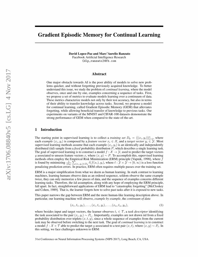
Figure 1: Left: ACC, BWT, and FWT for all datasets and methods. Right: evolution of the testaccuracy at the first task, as more tasks are learned.

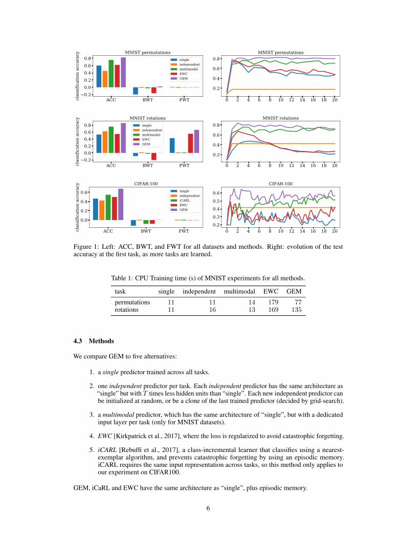
Table 1: CPU Training time (s) of MNIST experiments for all methods.

task single independent multimodal EWC GEM

permutations 11 11 14 179 77rotations 11 16 13 169 135

4.3 Methods

We compare GEM to five alternatives:

1. a single predictor trained across all tasks.

2. one independent predictor per task. Each independent predictor has the same architecture as“single” but with T times less hidden units than “single”. Each new independent predictor canbe initialized at random, or be a clone of the last trained predictor (decided by grid-search).

3. a multimodal predictor, which has the same architecture of “single”, but with a dedicatedinput layer per task (only for MNIST datasets).

4. EWC [Kirkpatrick et al., 2017], where the loss is regularized to avoid catastrophic forgetting.

5. iCARL [Rebuffi et al., 2017], a class-incremental learner that classifies using a nearest-exemplar algorithm, and prevents catastrophic forgetting by using an episodic memory.iCARL requires the same input representation across tasks, so this method only applies toour experiment on CIFAR100.

GEM, iCaRL and EWC have the same architecture as “single”, plus episodic memory.

6

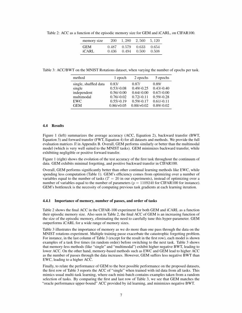
Table 2: ACC as a function of the episodic memory size for GEM and iCARL, on CIFAR100.

memory size 200 1, 280 2, 560 5, 120

GEM 0.487 0.579 0.633 0.654iCARL 0.436 0.494 0.500 0.508

Table 3: ACC/BWT on the MNIST Rotations dataset, when varying the number of epochs per task.

method 1 epoch 2 epochs 5 epochs

single, shuffled data 0.83/-0.00 0.87/-0.00 0.89/-0.00single 0.53/-0.08 0.49/-0.25 0.43/-0.40independent 0.56/-0.00 0.64/-0.00 0.67/-0.00multimodal 0.76/-0.02 0.72/-0.11 0.59/-0.28EWC 0.55/-0.19 0.59/-0.17 0.61/-0.11GEM 0.86/+0.05 0.88/+0.02 0.89/-0.02

4.4 Results

Figure 1 (left) summarizes the average accuracy (ACC, Equation 2), backward transfer (BWT,Equation 3) and forward transfer (FWT, Equation 4) for all datasets and methods. We provide the fullevaluation matrices R in Appendix B. Overall, GEM performs similarly or better than the multimodalmodel (which is very well suited to the MNIST tasks). GEM minimizes backward transfer, whileexhibiting negligible or positive forward transfer.

Figure 1 (right) shows the evolution of the test accuracy of the first task throughout the continuum ofdata. GEM exhibits minimal forgetting, and positive backward transfer in CIFAR100.

Overall, GEM performs significantly better than other continual learning methods like EWC, whilespending less computation (Table 1). GEM’s efficiency comes from optimizing over a number ofvariables equal to the number of tasks (T = 20 in our experiments), instead of optimizing over anumber of variables equal to the number of parameters (p = 1109240 for CIFAR100 for instance).GEM’s bottleneck is the necessity of computing previous task gradients at each learning iteration.

4.4.1 Importance of memory, number of passes, and order of tasks

Table 2 shows the final ACC in the CIFAR-100 experiment for both GEM and iCARL as a functiontheir episodic memory size. Also seen in Table 2, the final ACC of GEM is an increasing function ofthe size of the episodic memory, eliminating the need to carefully tune this hyper-parameter. GEMoutperforms iCARL for a wide range of memory sizes.

Table 3 illustrates the importance of memory as we do more than one pass through the data on theMNIST rotations experiment. Multiple training passe exacerbate the catastrophic forgetting problem.For instance, in the last column of Table 3 (except for the result in the first row), each model is shownexamples of a task five times (in random order) before switching to the next task. Table 3 showsthat memory-less methods (like “single” and “multimodal”) exhibit higher negative BWT, leading tolower ACC. On the other hand, memory-based methods such as EWC and GEM lead to higher ACCas the number of passes through the data increases. However, GEM suffers less negative BWT thanEWC, leading to a higher ACC.

Finally, to relate the performance of GEM to the best possible performance on the proposed datasets,the first row of Table 3 reports the ACC of “single” when trained with iid data from all tasks. Thismimics usual multi-task learning, where each mini-batch contains examples taken from a randomselection of tasks. By comparing the first and last row of Table 3, we see that GEM matches the“oracle performance upper-bound” ACC provided by iid learning, and minimizes negative BWT.

7

5 Related work

Continual learning [Ring, 1994], also called lifelong learning [Thrun, 1994, Thrun and Pratt, 2012,Thrun, 1998, 1996], considers learning through a sequence of tasks, where the learner has to retainknowledge about past tasks and leverage that knowledge to quickly acquire new skills. This learningsetting led to implementations [Carlson et al., 2010, Ruvolo and Eaton, 2013, Ring, 1997], andtheoretical investigations [Baxter, 2000, Balcan et al., 2015, Pentina and Urner, 2016], although thelatter ones have been restricted to linear models. In this work, we revisited continual learning butproposed to focus on the more realistic setting where examples are seen only once, memory is finite,and the learner is also provided with (potentially structured) task descriptors. Within this framework,we introduced a new set of metrics, a training and testing protocol, and a new algorithm, GEM, thatoutperforms the current state-of-the-art in terms of limiting forgetting.

The use of task descriptors is similar in spirit to recent work in Reinforcement Learning [Sutton et al.,2011, Schaul et al., 2015], where task or goal descriptors are also fed as input to the system. TheCommAI project [Mikolov et al., 2015, Baroni et al., 2017] shares our same motivations, but focuseson highly structured task descriptors, such as strings of text. In contrast, we focus on the problem ofcatastrophic forgetting [McCloskey and Cohen, 1989, French, 1999, Ratcliff, 1990, McClelland et al.,1995, Goodfellow et al., 2013].

Several approaches have been proposed to avoid catastrophic forgetting. The simplest approachin neural networks is to freeze early layers, while cloning and fine-tuning later layers on the newtask [Oquab et al., 2014] (which we considered in our “independent” baseline). This relates tomethods that leverage a modular structure of the network with primitives that can be shared acrosstasks [Rusu et al., 2016, Fernando et al., 2017, Aljundi et al., 2016, Denoyer and Gallinari, 2015,Eigen et al., 2014]. Unfortunately, it has been very hard to scale up these methods to lots of modulesand tasks, given the combinatorial number of compositions of modules.

Our approach is most similar to the regularization approaches that consider a single model, butmodify its learning objective to prevent catastrophic forgetting. Within this class of methods, thereare approaches that leverage “synaptic” memory [Kirkpatrick et al., 2017, Zenke et al., 2017], wherelearning rates are adjusted to minimize changes in parameters important for previous tasks. Otherapproaches are instead based on “episodic” memory [Jung et al., 2016, Li and Hoiem, 2016, RannenTriki et al., 2017, Rebuffi et al., 2017], where examples from previous tasks are stored and replayedto maintain predictions invariant by means of distillation [Hinton et al., 2015]. GEM is related tothese latter approaches but, unlike them, allows for positive backward transfer.

More generally, there are a variety of setups in the machine learning literature related to continuallearning. Multitask learning [Caruana, 1998] considers the problem of maximizing the performanceof a learning machine across a variety of tasks, but the setup assumes simultaneous access to all thetasks at once. Similarly, transfer learning [Pan and Yang, 2010] and domain adaptation [Ben-Davidet al., 2010] assume the simultaneous availability of multiple learning tasks, but focus at improvingthe performance at one of them in particular. Zero-shot learning [Lampert et al., 2009, Palatucciet al., 2009] and one-shot learning [Fei-Fei et al., 2003, Vinyals et al., 2016, Santoro et al., 2016,Bertinetto et al., 2016] aim at performing well on unseen tasks, but ignore the catastrophic forgettingof previously learned tasks. Curriculum learning considers learning a sequence of data [Bengio et al.,2009], or a sequence of tasks [Pentina et al., 2015], sorted by increasing difficulty.

6 Conclusion

We formalized the scenario of continual learning. First, we defined training and evaluation protocolsto assess the quality of models in terms of their accuracy, as well as their ability to transfer knowledgeforward and backward between tasks. Second, we introduced GEM, a simple model that leveragesan episodic memory to avoid forgetting and favor positive backward transfer. Our experimentsdemonstrate the competitive performance of GEM against the state-of-the-art.

GEM has three points for improvement. First, GEM does not leverage structured task descriptors,which may be exploited to obtain positive forward transfer (zero-shot learning). Second, we did notinvestigate advanced memory management (such as building coresets of tasks [Lucic et al., 2017]).Third, each GEM iteration requires one backward pass per task, increasing computation time. Theseare exciting research directions to extend learning machines beyond ERM, and to continuums of data.

8

Acknowledgements

We are grateful to M. Baroni, L. Bottou, M. Nickel, Y. Olivier and A. Szlam for their insight. We aregrateful to Martin Arjovsky for the QP interpretation of GEM.

ReferencesR. Aljundi, P. Chakravarty, and T. Tuytelaars. Expert gate: Lifelong learning with a network of experts. CVPR,

2016.

M.-F. Balcan, A. Blum, and S. Vempola. Efficient representations for lifelong learning and autoencoding. COLT,2015.

M. Baroni, A. Joulin, A. Jabri, G. Kruszewski, A. Lazaridou, K. Simonic, and T. Mikolov. CommAI: Evaluatingthe first steps towards a useful general AI. arXiv, 2017.

J. Baxter. A model of inductive bias learning. JAIR, 2000.

S. Ben-David, J. Blitzer, K. Crammer, A. Kulesza, F. Pereira, and J. Wortman Vaughan. A theory of learningfrom different domains. Machine Learning Journal, 2010.

Y. Bengio, J. Louradour, R. Collobert, and J. Weston. Curriculum learning. ICML, 2009.

L. Bertinetto, J. Henriques, J. Valmadre, P. Torr, and A. Vedaldi. Learning feed-forward one-shot learners. NIPS,2016.

A. Carlson, J. Betteridge, B. Kisiel, B. Settles, E. R. Hruschka, and T. M. Mitchell. Toward an architecture fornever-ending language learning. AAAI, 2010.

R. Caruana. Multitask learning. In Learning to learn. Springer, 1998.

L. Denoyer and P. Gallinari. Deep sequential neural networks. EWRL, 2015.

W. S. Dorn. Duality in quadratic programming. Quarterly of Applied Mathematics, 1960.

D. Eigen, I. Sutskever, and M. Ranzato. Learning factored representations in a deep mixture of experts. ICLR,2014.

L. Fei-Fei, R. Fergus, and P. Perona. A Bayesian approach to unsupervised one-shot learning of object categories.ICCV, 2003.

C. Fernando, D. Banarse, C. Blundell, Y. Zwols, D. Ha, A. A. Rusu, A. Pritzel, and D. Wierstra. PathNet:Evolution channels gradient descent in super neural networks. arXiv, 2017.

R. M. French. Catastrophic forgetting in connectionist networks. Trends in cognitive sciences, 1999.

I. J. Goodfellow, M. Mirza, D. Xiao, A. Courville, and Y. Bengio. An Empirical Investigation of CatastrophicForgetting in Gradient-Based Neural Networks. arXiv, 2013.

K. He, X. Zhang, S. Ren, and J. Sun. Deep residual learning for image recognition. arXiv, 2015.

G. Hinton, O. Vinyals, and J. Dean. Distilling the knowledge in a neural network. arXiv, 2015.

H. Jung, J. Ju, M. Jung, and J. Kim. Less-forgetting Learning in Deep Neural Networks. arXiv, 2016.

J. Kirkpatrick, R. Pascanu, N. Rabinowitz, J. Veness, G. Desjardins, A. A. Rusu, K. Milan, J. Quan, T. Ramalho,A. Grabska-Barwinska, et al. Overcoming catastrophic forgetting in neural networks. PNAS, 2017.

A. Krizhevsky. Learning multiple layers of features from tiny images. Technical report, Technical report,University of Toronto, 2009.

C. Lampert, H. Nickisch, and S. Harmeling. Learning to detect unseen object classes by between-class attributetransfer. CVPR, 2009.

Y. LeCun, C. Cortes, and C. J. Burges. The MNIST database of handwritten digits, 1998. URL http://yann.lecun.com/exdb/mnist/.

Z. Li and D. Hoiem. Learning without forgetting. ECCV, 2016.

9

M. Lucic, M. Faulkner , A. Krause, and D. Feldman. Training Mixture Models at Scale via Coresets. arXiv,2017.

J. L. McClelland, B. L. McNaughton, and R. C. O’reilly. Why there are complementary learning systems in thehippocampus and neocortex: insights from the successes and failures of connectionist models of learning andmemory. Psychological review, 1995.

M. McCloskey and N. J. Cohen. Catastrophic interference in connectionist networks: The sequential learningproblem. Psychology of learning and motivation, 1989.

T. Mikolov, A. Joulin, and M. Baroni. A roadmap towards machine intelligence. arXiv, 2015.

M. Oquab, L. Bottou, I. Laptev, and J. Sivic. Learning and transferring mid-level image representations usingconvolutional neural networks. CVPR, 2014.

M. Palatucci, D. A. Pomerleau, G. E. Hinton, and T. Mitchell. Zero-shot learning with semantic output codes.NIPS, 2009.

S. J. Pan and Q. Yang. A survey on transfer learning. TKDE, 2010.

A. Pentina and R. Urner. Lifelong learning with weighted majority votes. NIPS, 2016.

A. Pentina, V. Sharmanska, and C. H. Lampert. Curriculum learning of multiple tasks. CVPR, 2015.

J. Peters, P. Bühlmann, and N. Meinshausen. Causal inference by using invariant prediction: identification andconfidence intervals. Journal of the Royal Statistical Society, 2016.

A. Rannen Triki, R. Aljundi, M. B. Blaschko, and T. Tuytelaars. Encoder Based Lifelong Learning. arXiv, 2017.

R. Ratcliff. Connectionist models of recognition memory: Constraints imposed by learning and forgettingfunctions. Psychological review, 1990.

S.-A. Rebuffi, A. Kolesnikov, G. Sperl, and C. H. Lampert. iCaRL: Incremental classifier and representationlearning. CVPR, 2017.

M. B. Ring. Continual Learning in Reinforcement Environments. PhD thesis, University of Texas at Austin,Austin, Texas 78712, 1994.

M. B. Ring. CHILD: A first step towards continual learning. Machine Learning, 1997.

A. A. Rusu, N. C. Rabinowitz, G. Desjardins, H. Soyer, J. Kirkpatrick, K. Kavukcuoglu, R. Pascanu, andR. Hadsell. Progressive neural networks. NIPS, 2016.

P. Ruvolo and E. Eaton. ELLA: An Efficient Lifelong Learning Algorithm. ICML, 2013.

A. Santoro, S. Bartunov, M. Botvinick, D. Wierstra, and T. Lillicrap. One-shot learning with memory-augmentedneural networks. arXiv, 2016.

T. Schaul, D. Horgan, K. Gregor, and D. Silver. Universal value function approximators. ICML, 2015.

B. Scholkopf and A. J. Smola. Learning with kernels: support vector machines, regularization, optimization,and beyond. MIT press, 2001.

B. Schölkopf, D. Janzing, and D. Lopez-Paz. Causal and statistical learning. In Learning Theory and Approxi-mation. Oberwolfach Research Institute for Mathematics, 2016.

R. S. Sutton, J. Modayil, M. Delp, T. Degris, P. M. Pilarski, A. White, and D. Precup. Horde: A scalable real-timearchitecture for learning knowledge from unsupervised sensorimotor interaction. The 10th InternationalConference on Autonomous Agents and Multiagent Systems, 2011.

S. Thrun. A lifelong learning perspective for mobile robot control. Proceedings of the IEEE/RSJ/GI Conferenceon Intelligent Robots and Systems, 1994.

S. Thrun. Is learning the n-th thing any easier than learning the first? NIPS, 1996.

S. Thrun. Lifelong learning algorithms. In Learning to learn. Springer, 1998.

S. Thrun and L. Pratt. Learning to learn. Springer Science & Business Media, 2012.

V. Vapnik. Statistical learning theory. Wiley New York, 1998.

O. Vinyals, C. Blundell, T. Lillicrap, and D. Wierstra. Matching networks for one shot learning. NIPS, 2016.

F. Zenke, B. Poole, and S. Ganguli. Improved multitask learning through synaptic intelligence. arXiv, 2017.

10

A Hyper-parameter Selection

Here we report the hyper-parameter grids considered in our experiments. The best values for theMNIST rotations (rot), MNIST permutations (perm) and CIFAR-100 incremental (cifar) experimentsare noted accordingly in parenthesis. For more details, please refer to our implementation, linked inthe main text.

• single

– learning rate: [0.001, 0.003 (rot), 0.01, 0.03 (perm), 0.1, 0.3, 1.0 (cifar)]• independent

– learning rate: [0.001, 0.003, 0.01, 0.03 (perm), 0.1 (rot), 0.3 (cifar), 1.0]– finetune: [no, yes (rot, perm, cifar)]

• multimodal

– learning rate: [0.001, 0.003, 0.01, 0.03, 0.1 (rot, perm), 0.3, 1.0]• EWC

– learning rate: [0.001, 0.003, 0.01 (rot), 0.03, 0.1 (perm), 0.3, 1.0 (cifar)]– regularization: [1 (cifar), 3 (perm), 10, 30, 100, 300, 1000 (rot), 3000, 10000, 30000]

• iCARL

– learning rate: [0.001, 0.003, 0.01, 0.03, 0.1, 0.3, 1.0 (cifar)]– regularization: [0.1, 0.3, 1 (cifar), 3, 10, 30]– memory size: [200, 1280, 2560, 5120 (cifar)]

• GEM

– learning rate: [0.001, 0.003, 0.01, 0.03, 0.1 (rot, perm, cifar), 0.3, 1.0]– memory size: [5120 (rot, perm, cifar)]– γ: [0.0, 0.1, ..., 0.5 (rot, perm, cifar), ..., 1.0]

11

B Full experiments

In this section we report the evaluation matrices R for each model and dataset. The first row of eachmatrix (above the line) is the baseline test accuracy b̄ before training starts. The rest of entries (i, j)of the matrix R report the test accuracy of the j-th task just after finishing training the i-th task.

B.1 MNIST permutations

B.1.1 Model single0.1330 0.1199 0.1070 0.0825 0.0609 0.0832 0.1385 0.1123 0.0736 0.1190 0.0666 0.0890 0.0885 0.0723 0.1083 0.0524 0.0976 0.0871 0.1143 0.0743|0.7838 0.1264 0.0709 0.1142 0.0671 0.0928 0.0925 0.0878 0.0759 0.0832 0.0748 0.1057 0.0927 0.0770 0.0886 0.0995 0.1328 0.0839 0.1802 0.06090.7374 0.7939 0.0981 0.1496 0.0859 0.0626 0.1226 0.0666 0.1045 0.0596 0.0787 0.0938 0.0948 0.0737 0.0797 0.0670 0.1450 0.1062 0.1438 0.07140.6564 0.7196 0.7783 0.1177 0.0603 0.0908 0.1296 0.0654 0.1246 0.0894 0.0721 0.0798 0.0811 0.0631 0.0759 0.0726 0.1338 0.1265 0.1567 0.10390.5246 0.6359 0.7593 0.7790 0.0612 0.0864 0.1118 0.0815 0.1028 0.0900 0.0991 0.0773 0.0947 0.0948 0.0931 0.0930 0.1111 0.1027 0.1504 0.10030.6272 0.7265 0.7737 0.7695 0.7827 0.0981 0.0898 0.0530 0.1031 0.0760 0.0675 0.0569 0.0989 0.0698 0.0810 0.0483 0.1305 0.0819 0.1386 0.09610.6177 0.7317 0.7890 0.7860 0.7808 0.8135 0.1020 0.0668 0.1005 0.0648 0.0456 0.0705 0.0932 0.0858 0.1056 0.0797 0.1483 0.1039 0.1442 0.07880.6071 0.6620 0.7623 0.7540 0.7657 0.7838 0.8113 0.0991 0.1127 0.0957 0.0493 0.0916 0.0713 0.0804 0.1383 0.0639 0.1336 0.1192 0.1336 0.09210.5221 0.6675 0.7466 0.6990 0.7239 0.7707 0.8156 0.7909 0.1107 0.0858 0.0510 0.0764 0.0668 0.0849 0.1103 0.0441 0.1232 0.0996 0.1434 0.07440.5252 0.6347 0.6880 0.6490 0.7100 0.7478 0.7958 0.7595 0.8149 0.0981 0.0514 0.0843 0.0658 0.0922 0.1139 0.0529 0.1113 0.0846 0.1321 0.08970.4967 0.5864 0.6611 0.6384 0.6439 0.7252 0.7579 0.7433 0.7643 0.7761 0.0757 0.0799 0.0757 0.0864 0.0959 0.0685 0.1234 0.0733 0.1842 0.09300.4475 0.5803 0.6970 0.6617 0.6656 0.7274 0.7326 0.7567 0.7699 0.7763 0.8150 0.0869 0.0600 0.1025 0.1103 0.0537 0.1281 0.1026 0.2042 0.08850.5281 0.5656 0.6930 0.5233 0.6089 0.6503 0.7072 0.7421 0.7283 0.7588 0.7663 0.7865 0.0570 0.1119 0.1056 0.0495 0.1348 0.0943 0.1699 0.07890.5007 0.5260 0.6689 0.5819 0.5772 0.5277 0.6928 0.7165 0.7096 0.7229 0.7449 0.7382 0.8271 0.1264 0.1036 0.0706 0.1131 0.0985 0.1906 0.08200.4961 0.4526 0.6794 0.5465 0.5234 0.5238 0.6348 0.6833 0.6908 0.6886 0.7163 0.7292 0.7810 0.7952 0.1053 0.0661 0.1135 0.0942 0.2164 0.08060.4743 0.3400 0.5585 0.5611 0.5606 0.5228 0.6122 0.5523 0.6552 0.6740 0.6804 0.7231 0.7709 0.7340 0.8112 0.0747 0.1137 0.0811 0.1933 0.09880.4730 0.3533 0.5391 0.4235 0.4580 0.4516 0.6392 0.4629 0.6467 0.6725 0.6265 0.7099 0.7861 0.7021 0.7690 0.8066 0.0756 0.0953 0.1826 0.11470.4648 0.3295 0.5033 0.3883 0.4151 0.4542 0.5422 0.4495 0.5977 0.6719 0.5681 0.6966 0.7251 0.6391 0.7507 0.7260 0.7925 0.1094 0.1796 0.13890.4468 0.3238 0.4941 0.3709 0.4352 0.4632 0.5464 0.4534 0.6094 0.6366 0.6202 0.6787 0.6911 0.6615 0.7107 0.7206 0.8035 0.8109 0.1575 0.15260.4513 0.2867 0.4935 0.3826 0.4880 0.4347 0.5075 0.4067 0.5570 0.5492 0.5810 0.6007 0.6724 0.6000 0.7521 0.6801 0.7754 0.7353 0.8174 0.15320.4690 0.3482 0.5277 0.3742 0.4973 0.4406 0.5743 0.4568 0.6527 0.5518 0.6356 0.6396 0.6216 0.6537 0.7388 0.7072 0.8005 0.7300 0.8062 0.8107

Final Accuracy: 0.6018Backward: -0.1980Forward: 0.0093

B.1.2 Model independent0.0936 0.0995 0.0884 0.0893 0.0784 0.1000 0.1108 0.0965 0.1243 0.1048 0.0819 0.1115 0.0999 0.0762 0.1060 0.1260 0.0930 0.1075 0.1126 0.1092|0.1821 0.0995 0.0884 0.0893 0.0784 0.1000 0.1108 0.0965 0.1243 0.1048 0.0819 0.1115 0.0999 0.0762 0.1060 0.1260 0.0930 0.1075 0.1126 0.10920.1821 0.2601 0.0884 0.0893 0.0784 0.1000 0.1108 0.0965 0.1243 0.1048 0.0819 0.1115 0.0999 0.0762 0.1060 0.1260 0.0930 0.1075 0.1126 0.10920.1821 0.2601 0.3538 0.0893 0.0784 0.1000 0.1108 0.0965 0.1243 0.1048 0.0819 0.1115 0.0999 0.0762 0.1060 0.1260 0.0930 0.1075 0.1126 0.10920.1821 0.2601 0.3538 0.3089 0.0784 0.1000 0.1108 0.0965 0.1243 0.1048 0.0819 0.1115 0.0999 0.0762 0.1060 0.1260 0.0930 0.1075 0.1126 0.10920.1821 0.2601 0.3538 0.3089 0.4031 0.1000 0.1108 0.0965 0.1243 0.1048 0.0819 0.1115 0.0999 0.0762 0.1060 0.1260 0.0930 0.1075 0.1126 0.10920.1821 0.2601 0.3538 0.3089 0.4031 0.3267 0.1108 0.0965 0.1243 0.1048 0.0819 0.1115 0.0999 0.0762 0.1060 0.1260 0.0930 0.1075 0.1126 0.10920.1821 0.2601 0.3538 0.3089 0.4031 0.3267 0.4071 0.0965 0.1243 0.1048 0.0819 0.1115 0.0999 0.0762 0.1060 0.1260 0.0930 0.1075 0.1126 0.10920.1821 0.2601 0.3538 0.3089 0.4031 0.3267 0.4071 0.4030 0.1243 0.1048 0.0819 0.1115 0.0999 0.0762 0.1060 0.1260 0.0930 0.1075 0.1126 0.10920.1821 0.2601 0.3538 0.3089 0.4031 0.3267 0.4071 0.4030 0.4495 0.1048 0.0819 0.1115 0.0999 0.0762 0.1060 0.1260 0.0930 0.1075 0.1126 0.10920.1821 0.2601 0.3538 0.3089 0.4031 0.3267 0.4071 0.4030 0.4495 0.5276 0.0819 0.1115 0.0999 0.0762 0.1060 0.1260 0.0930 0.1075 0.1126 0.10920.1821 0.2601 0.3538 0.3089 0.4031 0.3267 0.4071 0.4030 0.4495 0.5276 0.4779 0.1115 0.0999 0.0762 0.1060 0.1260 0.0930 0.1075 0.1126 0.10920.1821 0.2601 0.3538 0.3089 0.4031 0.3267 0.4071 0.4030 0.4495 0.5276 0.4779 0.5357 0.0999 0.0762 0.1060 0.1260 0.0930 0.1075 0.1126 0.10920.1821 0.2601 0.3538 0.3089 0.4031 0.3267 0.4071 0.4030 0.4495 0.5276 0.4779 0.5357 0.5393 0.0762 0.1060 0.1260 0.0930 0.1075 0.1126 0.10920.1821 0.2601 0.3538 0.3089 0.4031 0.3267 0.4071 0.4030 0.4495 0.5276 0.4779 0.5357 0.5393 0.5755 0.1060 0.1260 0.0930 0.1075 0.1126 0.10920.1821 0.2601 0.3538 0.3089 0.4031 0.3267 0.4071 0.4030 0.4495 0.5276 0.4779 0.5357 0.5393 0.5755 0.5592 0.1260 0.0930 0.1075 0.1126 0.10920.1821 0.2601 0.3538 0.3089 0.4031 0.3267 0.4071 0.4030 0.4495 0.5276 0.4779 0.5357 0.5393 0.5755 0.5592 0.5145 0.0930 0.1075 0.1126 0.10920.1821 0.2601 0.3538 0.3089 0.4031 0.3267 0.4071 0.4030 0.4495 0.5276 0.4779 0.5357 0.5393 0.5755 0.5592 0.5145 0.5553 0.1075 0.1126 0.10920.1821 0.2601 0.3538 0.3089 0.4031 0.3267 0.4071 0.4030 0.4495 0.5276 0.4779 0.5357 0.5393 0.5755 0.5592 0.5145 0.5553 0.5675 0.1126 0.10920.1821 0.2601 0.3538 0.3089 0.4031 0.3267 0.4071 0.4030 0.4495 0.5276 0.4779 0.5357 0.5393 0.5755 0.5592 0.5145 0.5553 0.5675 0.5252 0.10920.1821 0.2601 0.3538 0.3089 0.4031 0.3267 0.4071 0.4030 0.4495 0.5276 0.4779 0.5357 0.5393 0.5755 0.5592 0.5145 0.5553 0.5675 0.5252 0.5739

Final Accuracy: 0.4523Backward: 0.0000Forward: 0.0000

12

B.1.3 Model multimodal

0.0749 0.1152 0.0601 0.0885 0.0826 0.0856 0.0925 0.0703 0.1079 0.0891 0.1029 0.1092 0.0866 0.1014 0.1575 0.1005 0.1083 0.1038 0.0857 0.0759|0.6871 0.1306 0.1402 0.1209 0.1108 0.1135 0.1195 0.1066 0.1368 0.1217 0.0605 0.1168 0.1094 0.0970 0.1150 0.1322 0.1471 0.1243 0.1054 0.15670.7123 0.8211 0.1344 0.1197 0.0923 0.1155 0.1402 0.1030 0.1346 0.1424 0.1030 0.1329 0.0910 0.0875 0.1437 0.1245 0.1094 0.0865 0.0771 0.17680.7716 0.8180 0.8163 0.1208 0.0871 0.1154 0.1308 0.0916 0.1482 0.1238 0.1092 0.1159 0.1122 0.0868 0.1192 0.1221 0.1518 0.0981 0.0692 0.13620.7451 0.7961 0.7976 0.7757 0.0883 0.1152 0.1235 0.0849 0.1612 0.1265 0.0976 0.1177 0.1112 0.0914 0.1177 0.1072 0.1681 0.0847 0.0724 0.14950.6841 0.7759 0.7569 0.7709 0.7887 0.1147 0.1296 0.0749 0.1561 0.1259 0.0958 0.1216 0.1104 0.0878 0.1261 0.1410 0.1496 0.1009 0.0741 0.17830.7344 0.8274 0.8126 0.7832 0.8041 0.8057 0.1145 0.0647 0.1449 0.1446 0.0826 0.1047 0.0862 0.0896 0.1324 0.1362 0.1217 0.0773 0.0878 0.16400.7679 0.8373 0.8228 0.7891 0.8117 0.7830 0.8464 0.0673 0.1467 0.1437 0.0831 0.1015 0.0864 0.0880 0.1340 0.1264 0.1212 0.0763 0.0819 0.15320.7327 0.8004 0.7749 0.7608 0.7858 0.8231 0.8253 0.7830 0.1472 0.1343 0.1082 0.1209 0.1179 0.1115 0.1159 0.1263 0.1357 0.0862 0.0988 0.18240.7606 0.7713 0.7570 0.7962 0.7871 0.8118 0.8393 0.7462 0.7877 0.1288 0.0877 0.1018 0.0819 0.0664 0.1287 0.1060 0.1107 0.0679 0.0801 0.11690.7213 0.7791 0.7889 0.7818 0.7401 0.7756 0.8084 0.7793 0.7996 0.7521 0.0575 0.1151 0.0893 0.0667 0.1280 0.1092 0.1194 0.0717 0.0732 0.13650.6891 0.7691 0.7889 0.7772 0.7392 0.8103 0.7917 0.7584 0.8111 0.7634 0.8079 0.0984 0.0758 0.0815 0.1398 0.1195 0.1019 0.0849 0.0783 0.11040.7357 0.8039 0.7822 0.7710 0.7673 0.8090 0.7918 0.8125 0.7698 0.7689 0.7859 0.7383 0.0858 0.0681 0.1369 0.1135 0.1170 0.0762 0.0780 0.13300.7082 0.7856 0.7612 0.7351 0.7639 0.7871 0.7741 0.8013 0.7273 0.7818 0.7458 0.6813 0.8387 0.0607 0.1368 0.1084 0.1106 0.0686 0.0696 0.11950.7344 0.7662 0.7261 0.7582 0.7844 0.8025 0.8005 0.7910 0.7397 0.7952 0.7445 0.6660 0.8303 0.6274 0.1447 0.1076 0.1078 0.0711 0.0655 0.10390.7347 0.7716 0.7370 0.7814 0.7901 0.7909 0.8188 0.7887 0.7521 0.7739 0.7428 0.6771 0.8373 0.6218 0.8413 0.1006 0.0890 0.0667 0.0688 0.09220.7544 0.7908 0.7497 0.8055 0.7880 0.8026 0.8243 0.7854 0.7665 0.7741 0.7767 0.7199 0.8211 0.6111 0.8349 0.7976 0.0985 0.0813 0.0811 0.09340.7579 0.7631 0.7103 0.7976 0.7695 0.7876 0.8066 0.7507 0.7860 0.7708 0.7680 0.6620 0.7952 0.5357 0.8083 0.7646 0.7769 0.0813 0.0730 0.09900.6829 0.7751 0.7282 0.7604 0.7526 0.7427 0.7484 0.7788 0.7369 0.7357 0.7413 0.6109 0.8131 0.5895 0.8224 0.7750 0.8211 0.7871 0.0771 0.08810.7128 0.7917 0.7226 0.7779 0.7647 0.7361 0.8046 0.7454 0.7549 0.7559 0.7757 0.6850 0.8092 0.5882 0.8022 0.7528 0.8176 0.7988 0.7844 0.09020.7068 0.7832 0.7106 0.7704 0.7642 0.7382 0.7866 0.7218 0.7623 0.7496 0.7829 0.7072 0.8015 0.5605 0.7974 0.7645 0.8115 0.8045 0.7904 0.8077

Final Accuracy: 0.7561Backward: -0.0275Forward: 0.0059

B.1.4 Model EWC

0.1330 0.1199 0.1070 0.0825 0.0609 0.0832 0.1385 0.1123 0.0736 0.1190 0.0666 0.0890 0.0885 0.0723 0.1083 0.0524 0.0976 0.0871 0.1143 0.0743|0.7289 0.1426 0.0776 0.1272 0.0637 0.0582 0.0944 0.0961 0.0691 0.0794 0.0822 0.1426 0.0953 0.0792 0.0885 0.1094 0.1328 0.0987 0.1507 0.09760.7396 0.8305 0.0703 0.1585 0.0749 0.0545 0.1558 0.0789 0.1076 0.0857 0.0699 0.1361 0.0953 0.0581 0.0704 0.0850 0.1241 0.1280 0.1382 0.10120.6882 0.7731 0.8274 0.1326 0.0496 0.0917 0.1571 0.0767 0.1015 0.1061 0.0790 0.0712 0.0622 0.0632 0.0982 0.0803 0.1535 0.1088 0.1399 0.11340.6361 0.7054 0.7915 0.7780 0.0733 0.0681 0.1446 0.0587 0.0888 0.1046 0.1141 0.0731 0.1008 0.0928 0.0968 0.1183 0.1263 0.1112 0.1130 0.11410.6625 0.7168 0.7724 0.7663 0.7665 0.0807 0.1015 0.0576 0.1105 0.0735 0.0783 0.0703 0.0951 0.0744 0.0658 0.0775 0.1378 0.0938 0.1127 0.12260.6667 0.6854 0.7791 0.7800 0.7795 0.7990 0.0850 0.0597 0.1037 0.0543 0.0515 0.0714 0.0566 0.1021 0.0906 0.0791 0.1603 0.0997 0.1140 0.11080.6193 0.6901 0.7954 0.7871 0.7436 0.7666 0.8404 0.0960 0.1232 0.0752 0.0660 0.0898 0.0460 0.0707 0.1058 0.0696 0.1410 0.1144 0.0948 0.11750.5454 0.6454 0.7321 0.7166 0.7331 0.7609 0.8361 0.7918 0.1004 0.0805 0.0540 0.0902 0.0451 0.1068 0.0924 0.0720 0.1259 0.1018 0.0988 0.10010.5594 0.6857 0.7414 0.6629 0.7248 0.6523 0.7804 0.7862 0.7973 0.0906 0.0790 0.0921 0.0481 0.1199 0.0959 0.0650 0.1147 0.0790 0.1291 0.11430.5880 0.6145 0.7121 0.7267 0.6943 0.6630 0.7527 0.7069 0.7303 0.7930 0.0978 0.0607 0.0488 0.1357 0.0969 0.0989 0.1437 0.0632 0.1132 0.11480.5455 0.6000 0.7029 0.6885 0.6554 0.6926 0.6618 0.7296 0.7446 0.7713 0.8005 0.0739 0.0583 0.1253 0.1082 0.0656 0.1396 0.1021 0.1393 0.10660.5770 0.6049 0.6553 0.5227 0.6169 0.5683 0.6525 0.5805 0.6772 0.6869 0.7180 0.7147 0.0421 0.1338 0.0964 0.0602 0.1148 0.1037 0.1060 0.08780.5668 0.6023 0.6847 0.6257 0.5574 0.6179 0.6576 0.5748 0.5917 0.7406 0.7422 0.7544 0.8085 0.1488 0.1065 0.0981 0.0996 0.0986 0.0949 0.07220.5325 0.5731 0.6141 0.4784 0.5395 0.5387 0.6384 0.5310 0.6705 0.6309 0.6515 0.7252 0.7926 0.7110 0.1178 0.0927 0.0911 0.1137 0.0887 0.09770.5039 0.5394 0.6175 0.5436 0.5573 0.5783 0.5886 0.4870 0.6058 0.6844 0.6531 0.7011 0.7850 0.6647 0.8235 0.0619 0.0990 0.0922 0.0998 0.11720.5799 0.4831 0.5988 0.4822 0.5807 0.4963 0.6100 0.4051 0.6081 0.6858 0.5913 0.7020 0.7989 0.6506 0.7815 0.8030 0.0902 0.0877 0.0912 0.12500.5399 0.4113 0.5397 0.4447 0.5240 0.5427 0.5627 0.3753 0.5512 0.6142 0.4868 0.7001 0.7361 0.6206 0.6931 0.7176 0.7411 0.1161 0.1373 0.13470.5427 0.5133 0.5789 0.5249 0.6101 0.5422 0.5875 0.4113 0.6144 0.5876 0.5636 0.6325 0.7244 0.6313 0.6796 0.7146 0.7886 0.7659 0.1224 0.11800.5085 0.5428 0.6279 0.5754 0.5676 0.5175 0.6138 0.4533 0.6017 0.5632 0.6322 0.5923 0.6966 0.6234 0.6764 0.6761 0.7688 0.7045 0.7836 0.11220.4839 0.5742 0.5863 0.5711 0.5760 0.5578 0.5912 0.4302 0.6911 0.5543 0.5981 0.6211 0.6812 0.6415 0.6357 0.5967 0.7709 0.7132 0.7234 0.7715

Final Accuracy: 0.6185Backward: -0.1653Forward: 0.0054

B.1.5 Model GEM

0.1330 0.1199 0.1070 0.0825 0.0609 0.0832 0.1385 0.1123 0.0736 0.1190 0.0666 0.0890 0.0885 0.0723 0.1083 0.0524 0.0976 0.0871 0.1143 0.0743|0.7289 0.1426 0.0776 0.1272 0.0637 0.0582 0.0944 0.0961 0.0691 0.0794 0.0822 0.1426 0.0953 0.0792 0.0885 0.1094 0.1328 0.0987 0.1507 0.09760.8158 0.8356 0.0601 0.1668 0.0708 0.0624 0.1524 0.0836 0.0994 0.0757 0.0802 0.1278 0.1056 0.0634 0.0625 0.0924 0.1193 0.1390 0.1392 0.10310.8134 0.8302 0.8407 0.1509 0.0539 0.0987 0.1566 0.0785 0.1134 0.1025 0.0659 0.0808 0.0746 0.0593 0.0883 0.0759 0.1764 0.1191 0.1253 0.10670.7732 0.7940 0.8306 0.7605 0.0622 0.0789 0.1374 0.0669 0.1172 0.0735 0.0979 0.0488 0.0877 0.0802 0.0713 0.1161 0.1434 0.1216 0.1295 0.10320.8079 0.8283 0.8478 0.8328 0.7798 0.0797 0.0918 0.0598 0.1376 0.0753 0.0704 0.0516 0.0986 0.0573 0.0549 0.0802 0.1815 0.1077 0.1249 0.12790.8262 0.8296 0.8296 0.8471 0.8472 0.8093 0.0888 0.0661 0.0942 0.0890 0.0572 0.0487 0.0707 0.0954 0.0957 0.0793 0.1793 0.1086 0.1306 0.10490.8109 0.8214 0.8132 0.8374 0.8445 0.8429 0.8297 0.0984 0.0999 0.0971 0.0699 0.0608 0.0662 0.0722 0.0910 0.0814 0.1720 0.1175 0.1218 0.11650.8098 0.8185 0.8268 0.8388 0.8275 0.8391 0.8587 0.7566 0.1019 0.1059 0.0751 0.0727 0.0563 0.1015 0.1116 0.0856 0.1505 0.0991 0.1793 0.11440.8260 0.8247 0.8447 0.8290 0.8468 0.8362 0.8517 0.8246 0.8219 0.1096 0.0734 0.0662 0.0595 0.1137 0.0923 0.0855 0.1417 0.1073 0.1398 0.11560.8202 0.8264 0.8237 0.8271 0.8462 0.8458 0.8462 0.8307 0.8574 0.8142 0.0670 0.0787 0.0691 0.0957 0.0950 0.0975 0.1403 0.0828 0.1587 0.12040.8213 0.8137 0.8228 0.8257 0.8352 0.8517 0.8422 0.8296 0.8515 0.8559 0.8041 0.0808 0.0628 0.1036 0.1005 0.0805 0.1351 0.1107 0.1509 0.10260.7878 0.8073 0.8088 0.7913 0.8250 0.8290 0.8328 0.8196 0.8388 0.8343 0.8172 0.7556 0.0686 0.1228 0.0976 0.0922 0.1308 0.1180 0.1360 0.08700.8114 0.8181 0.8149 0.8128 0.8328 0.8273 0.8407 0.8254 0.8487 0.8551 0.8339 0.8550 0.8224 0.1212 0.1038 0.1207 0.1185 0.0969 0.1461 0.09280.7982 0.8191 0.8133 0.8094 0.8350 0.8343 0.8495 0.8186 0.8473 0.8566 0.8279 0.8552 0.8505 0.7850 0.1130 0.1232 0.1264 0.0816 0.1328 0.10510.8044 0.8217 0.8170 0.8198 0.8429 0.8240 0.8490 0.8147 0.8498 0.8568 0.8334 0.8551 0.8489 0.8442 0.8291 0.1096 0.1197 0.0890 0.1746 0.10450.8150 0.8198 0.8126 0.8250 0.8348 0.8281 0.8476 0.8191 0.8487 0.8551 0.8343 0.8575 0.8520 0.8447 0.8517 0.8155 0.1148 0.0896 0.1269 0.12690.8100 0.8164 0.8030 0.8162 0.8355 0.8242 0.8455 0.8149 0.8348 0.8531 0.8311 0.8541 0.8528 0.8411 0.8558 0.8367 0.8253 0.1083 0.1452 0.10350.8031 0.8092 0.8047 0.8170 0.8294 0.8103 0.8421 0.8087 0.8384 0.8479 0.8379 0.8399 0.8467 0.8413 0.8478 0.8377 0.8501 0.8287 0.1335 0.11020.7999 0.8107 0.8038 0.8033 0.8168 0.8067 0.8433 0.8044 0.8309 0.8397 0.8355 0.8349 0.8419 0.8320 0.8379 0.8363 0.8421 0.8369 0.7689 0.11190.8024 0.8063 0.7966 0.8045 0.8199 0.8153 0.8430 0.8009 0.8317 0.8494 0.8304 0.8391 0.8431 0.8341 0.8426 0.8226 0.8461 0.8436 0.8350 0.8141

Final Accuracy: 0.8260Backward: 0.0247Forward: 0.0088

13

B.2 MNIST rotations

B.2.1 Model single0.0903 0.0957 0.0843 0.0882 0.0910 0.0847 0.0998 0.0992 0.0906 0.0756 0.0743 0.0781 0.0839 0.0873 0.0778 0.0810 0.0780 0.0791 0.0884 0.0867|0.2777 0.2559 0.2387 0.2382 0.2057 0.1597 0.1548 0.1284 0.1106 0.0912 0.0881 0.0889 0.1082 0.1030 0.0950 0.1011 0.1059 0.1130 0.1263 0.14900.4166 0.4466 0.3915 0.3657 0.3048 0.2447 0.2062 0.1701 0.1476 0.1358 0.1285 0.1236 0.1473 0.1221 0.1164 0.1212 0.1074 0.1174 0.1394 0.16460.4598 0.5531 0.5332 0.4883 0.4369 0.3510 0.2676 0.2098 0.1822 0.1580 0.1467 0.1379 0.1568 0.1279 0.1240 0.1280 0.1167 0.1215 0.1426 0.16420.4760 0.5879 0.5823 0.5779 0.5265 0.4513 0.3448 0.2649 0.2321 0.1786 0.1593 0.1441 0.1541 0.1301 0.1241 0.1240 0.1234 0.1334 0.1529 0.16770.4619 0.6080 0.6358 0.6383 0.6069 0.5365 0.4179 0.3122 0.2670 0.1996 0.1727 0.1534 0.1486 0.1271 0.1290 0.1296 0.1319 0.1426 0.1701 0.18920.4522 0.6096 0.6652 0.6865 0.6793 0.6383 0.5041 0.3951 0.3331 0.2389 0.1984 0.1681 0.1609 0.1388 0.1443 0.1396 0.1465 0.1489 0.1731 0.19160.4191 0.5759 0.6415 0.6779 0.6902 0.6793 0.6057 0.5175 0.4500 0.3221 0.2554 0.1986 0.1720 0.1410 0.1420 0.1406 0.1486 0.1547 0.1770 0.20250.4160 0.5657 0.6248 0.6618 0.7004 0.7245 0.6977 0.6576 0.6200 0.4765 0.3857 0.2642 0.2134 0.1595 0.1524 0.1504 0.1471 0.1562 0.1726 0.19650.3671 0.5139 0.5866 0.6303 0.6699 0.7021 0.7016 0.6990 0.6878 0.5734 0.4855 0.3443 0.2578 0.1729 0.1503 0.1441 0.1446 0.1525 0.1738 0.19360.3269 0.4819 0.5596 0.6152 0.6666 0.7057 0.7219 0.7343 0.7272 0.6526 0.5712 0.4225 0.3191 0.2081 0.1758 0.1648 0.1479 0.1543 0.1665 0.17960.3098 0.4567 0.5334 0.5945 0.6441 0.6876 0.7189 0.7482 0.7576 0.7061 0.6630 0.5231 0.4143 0.2643 0.2052 0.1907 0.1557 0.1607 0.1692 0.18770.2879 0.4181 0.4965 0.5614 0.6175 0.6678 0.7104 0.7449 0.7595 0.7329 0.7159 0.6327 0.5347 0.3718 0.2821 0.2556 0.1917 0.1882 0.1873 0.19770.2797 0.4064 0.4695 0.5275 0.5915 0.6495 0.6925 0.7310 0.7486 0.7341 0.7398 0.6979 0.6550 0.5034 0.3892 0.3615 0.2490 0.2378 0.2121 0.20790.2545 0.3551 0.4139 0.4677 0.5308 0.5871 0.6519 0.6939 0.7186 0.7197 0.7367 0.7369 0.7174 0.6270 0.5141 0.4821 0.3397 0.3041 0.2487 0.23460.2613 0.3557 0.3999 0.4496 0.5069 0.5534 0.6194 0.6540 0.6815 0.6885 0.7134 0.7317 0.7440 0.7064 0.6553 0.6275 0.4707 0.4288 0.3217 0.28040.2485 0.3330 0.3686 0.4169 0.4739 0.5138 0.5891 0.6245 0.6503 0.6715 0.6947 0.7258 0.7536 0.7440 0.7201 0.7051 0.5773 0.5326 0.3963 0.34440.2468 0.3107 0.3275 0.3603 0.4160 0.4402 0.5168 0.5672 0.5917 0.6307 0.6577 0.7025 0.7393 0.7559 0.7551 0.7474 0.6757 0.6328 0.5115 0.45790.2243 0.2914 0.3098 0.3437 0.3873 0.4008 0.4748 0.5190 0.5470 0.5950 0.6142 0.6730 0.7173 0.7530 0.7723 0.7738 0.7373 0.7128 0.5946 0.53450.2055 0.2771 0.2953 0.3319 0.3715 0.3848 0.4420 0.4860 0.5122 0.5549 0.5759 0.6355 0.6768 0.7149 0.7563 0.7592 0.7544 0.7478 0.6940 0.63900.2136 0.2710 0.2837 0.3126 0.3460 0.3508 0.4033 0.4461 0.4702 0.5237 0.5408 0.6021 0.6513 0.6987 0.7481 0.7590 0.7708 0.7772 0.7434 0.7023

Final Accuracy: 0.5307Backward: -0.0896Forward: 0.4254

B.2.2 Model independent0.1013 0.0910 0.1049 0.0761 0.0976 0.1071 0.0960 0.0890 0.0815 0.1172 0.0938 0.1231 0.1140 0.0874 0.0995 0.1005 0.1075 0.0919 0.0942 0.1790|0.4221 0.0910 0.1049 0.0761 0.0976 0.1071 0.0960 0.0890 0.0815 0.1172 0.0938 0.1231 0.1140 0.0874 0.0995 0.1005 0.1075 0.0919 0.0942 0.17900.4221 0.5266 0.1049 0.0761 0.0976 0.1071 0.0960 0.0890 0.0815 0.1172 0.0938 0.1231 0.1140 0.0874 0.0995 0.1005 0.1075 0.0919 0.0942 0.17900.4221 0.5266 0.5069 0.0761 0.0976 0.1071 0.0960 0.0890 0.0815 0.1172 0.0938 0.1231 0.1140 0.0874 0.0995 0.1005 0.1075 0.0919 0.0942 0.17900.4221 0.5266 0.5069 0.5967 0.0976 0.1071 0.0960 0.0890 0.0815 0.1172 0.0938 0.1231 0.1140 0.0874 0.0995 0.1005 0.1075 0.0919 0.0942 0.17900.4221 0.5266 0.5069 0.5967 0.5091 0.1071 0.0960 0.0890 0.0815 0.1172 0.0938 0.1231 0.1140 0.0874 0.0995 0.1005 0.1075 0.0919 0.0942 0.17900.4221 0.5266 0.5069 0.5967 0.5091 0.6481 0.0960 0.0890 0.0815 0.1172 0.0938 0.1231 0.1140 0.0874 0.0995 0.1005 0.1075 0.0919 0.0942 0.17900.4221 0.5266 0.5069 0.5967 0.5091 0.6481 0.6278 0.0890 0.0815 0.1172 0.0938 0.1231 0.1140 0.0874 0.0995 0.1005 0.1075 0.0919 0.0942 0.17900.4221 0.5266 0.5069 0.5967 0.5091 0.6481 0.6278 0.5654 0.0815 0.1172 0.0938 0.1231 0.1140 0.0874 0.0995 0.1005 0.1075 0.0919 0.0942 0.17900.4221 0.5266 0.5069 0.5967 0.5091 0.6481 0.6278 0.5654 0.5874 0.1172 0.0938 0.1231 0.1140 0.0874 0.0995 0.1005 0.1075 0.0919 0.0942 0.17900.4221 0.5266 0.5069 0.5967 0.5091 0.6481 0.6278 0.5654 0.5874 0.5711 0.0938 0.1231 0.1140 0.0874 0.0995 0.1005 0.1075 0.0919 0.0942 0.17900.4221 0.5266 0.5069 0.5967 0.5091 0.6481 0.6278 0.5654 0.5874 0.5711 0.6846 0.1231 0.1140 0.0874 0.0995 0.1005 0.1075 0.0919 0.0942 0.17900.4221 0.5266 0.5069 0.5967 0.5091 0.6481 0.6278 0.5654 0.5874 0.5711 0.6846 0.6723 0.1140 0.0874 0.0995 0.1005 0.1075 0.0919 0.0942 0.17900.4221 0.5266 0.5069 0.5967 0.5091 0.6481 0.6278 0.5654 0.5874 0.5711 0.6846 0.6723 0.6533 0.0874 0.0995 0.1005 0.1075 0.0919 0.0942 0.17900.4221 0.5266 0.5069 0.5967 0.5091 0.6481 0.6278 0.5654 0.5874 0.5711 0.6846 0.6723 0.6533 0.5998 0.0995 0.1005 0.1075 0.0919 0.0942 0.17900.4221 0.5266 0.5069 0.5967 0.5091 0.6481 0.6278 0.5654 0.5874 0.5711 0.6846 0.6723 0.6533 0.5998 0.7046 0.1005 0.1075 0.0919 0.0942 0.17900.4221 0.5266 0.5069 0.5967 0.5091 0.6481 0.6278 0.5654 0.5874 0.5711 0.6846 0.6723 0.6533 0.5998 0.7046 0.6965 0.1075 0.0919 0.0942 0.17900.4221 0.5266 0.5069 0.5967 0.5091 0.6481 0.6278 0.5654 0.5874 0.5711 0.6846 0.6723 0.6533 0.5998 0.7046 0.6965 0.7011 0.0919 0.0942 0.17900.4221 0.5266 0.5069 0.5967 0.5091 0.6481 0.6278 0.5654 0.5874 0.5711 0.6846 0.6723 0.6533 0.5998 0.7046 0.6965 0.7011 0.7532 0.0942 0.17900.4221 0.5266 0.5069 0.5967 0.5091 0.6481 0.6278 0.5654 0.5874 0.5711 0.6846 0.6723 0.6533 0.5998 0.7046 0.6965 0.7011 0.7532 0.7424 0.17900.4221 0.5266 0.5069 0.5967 0.5091 0.6481 0.6278 0.5654 0.5874 0.5711 0.6846 0.6723 0.6533 0.5998 0.7046 0.6965 0.7011 0.7532 0.7424 0.7131

Final Accuracy: 0.6241Backward: 0.0000Forward: 0.0000

B.2.3 Model multimodal0.0910 0.0870 0.0943 0.0850 0.1043 0.1102 0.0820 0.0696 0.1339 0.0871 0.0946 0.0901 0.0961 0.0506 0.0991 0.0819 0.1018 0.0846 0.0778 0.1116|0.6383 0.1237 0.1273 0.1238 0.1322 0.1184 0.1173 0.1289 0.1152 0.1068 0.1253 0.1499 0.1202 0.1165 0.1327 0.1088 0.1264 0.0729 0.1397 0.10970.6893 0.8122 0.1502 0.1124 0.1077 0.1306 0.1124 0.1104 0.1749 0.0445 0.1239 0.1555 0.0726 0.1460 0.1044 0.0768 0.1344 0.0667 0.0936 0.11400.7519 0.7990 0.7989 0.1042 0.0798 0.1415 0.0978 0.0843 0.1692 0.0656 0.1042 0.1048 0.0994 0.1430 0.0601 0.0966 0.1270 0.0688 0.0754 0.13100.7601 0.7709 0.7155 0.7898 0.0860 0.1465 0.0952 0.0756 0.1799 0.0509 0.1106 0.1279 0.1067 0.1275 0.0607 0.0947 0.1293 0.0746 0.0888 0.14420.6484 0.7890 0.7966 0.8229 0.7745 0.1345 0.0966 0.1006 0.1790 0.0381 0.1081 0.1532 0.1041 0.1488 0.0745 0.0627 0.1352 0.0588 0.1351 0.12400.7081 0.7838 0.8047 0.8242 0.7983 0.8155 0.1031 0.1075 0.1842 0.0345 0.0954 0.1556 0.1202 0.1501 0.0727 0.0764 0.1280 0.0617 0.1047 0.10410.7024 0.7591 0.8092 0.8247 0.7894 0.8185 0.8534 0.0859 0.1825 0.0374 0.0848 0.1266 0.1013 0.1776 0.0483 0.0851 0.1186 0.0583 0.1074 0.09560.6513 0.7391 0.7529 0.8224 0.7751 0.7736 0.7943 0.8205 0.1899 0.0575 0.1190 0.1675 0.1221 0.1437 0.1153 0.0963 0.1484 0.0676 0.1175 0.11820.6982 0.7214 0.7352 0.8050 0.7633 0.7760 0.7679 0.7914 0.7938 0.0640 0.0981 0.1094 0.1005 0.1551 0.0467 0.1016 0.1342 0.0753 0.0884 0.10250.7137 0.7398 0.7571 0.8232 0.7566 0.8061 0.8019 0.8078 0.7705 0.7824 0.1036 0.1169 0.1033 0.1426 0.0397 0.0948 0.1914 0.0688 0.0853 0.10820.6852 0.7492 0.7546 0.8247 0.7722 0.8114 0.8113 0.7814 0.7905 0.7918 0.8244 0.1497 0.1274 0.1331 0.0725 0.0907 0.1988 0.0564 0.0846 0.09660.6730 0.7220 0.7138 0.7417 0.7212 0.8037 0.7353 0.7522 0.7307 0.8016 0.7666 0.7150 0.1374 0.1520 0.0688 0.0977 0.1953 0.0512 0.0916 0.08550.6708 0.7275 0.7316 0.7717 0.7189 0.8170 0.7439 0.7635 0.7686 0.7958 0.7602 0.7145 0.8476 0.1562 0.0531 0.0954 0.1447 0.0565 0.0712 0.06760.7254 0.6934 0.6972 0.7631 0.7215 0.7612 0.7491 0.7587 0.7416 0.7863 0.7467 0.6608 0.8258 0.6332 0.0521 0.0971 0.1256 0.0805 0.0856 0.09700.7337 0.6945 0.7183 0.7578 0.7289 0.7751 0.7479 0.7891 0.7405 0.8019 0.7546 0.6818 0.8461 0.6459 0.8378 0.1011 0.1223 0.0799 0.0763 0.09450.7242 0.6911 0.7217 0.7509 0.7299 0.7866 0.7370 0.7865 0.7550 0.8301 0.7717 0.6701 0.8528 0.6085 0.8414 0.8089 0.1177 0.0786 0.0751 0.09970.7510 0.7034 0.7479 0.7737 0.7465 0.7734 0.7507 0.8094 0.7728 0.8020 0.7903 0.6261 0.8367 0.6149 0.8214 0.7959 0.7532 0.0788 0.0762 0.09280.7208 0.6948 0.7312 0.7529 0.7133 0.7838 0.7536 0.8028 0.7382 0.7821 0.7730 0.6797 0.8350 0.6902 0.8278 0.7852 0.7852 0.7722 0.0750 0.07580.6976 0.7028 0.7227 0.7413 0.6956 0.7953 0.7429 0.8143 0.7494 0.7935 0.7792 0.6846 0.8354 0.6694 0.8254 0.7987 0.7890 0.7792 0.7901 0.08340.7065 0.7008 0.7246 0.7463 0.6862 0.7965 0.7323 0.8055 0.7398 0.7872 0.7736 0.6983 0.8370 0.6515 0.8280 0.7981 0.7994 0.7817 0.7832 0.7928

Final Accuracy: 0.7585Backward: -0.0243Forward: 0.0177

14

B.2.4 Model EWC0.0903 0.0957 0.0843 0.0882 0.0910 0.0847 0.0998 0.0992 0.0906 0.0756 0.0743 0.0781 0.0839 0.0873 0.0778 0.0810 0.0780 0.0791 0.0884 0.0867|0.5388 0.4506 0.3594 0.3211 0.2657 0.2081 0.1768 0.1425 0.1281 0.1229 0.1250 0.1321 0.1629 0.1452 0.1390 0.1385 0.1452 0.1508 0.1690 0.18310.6677 0.7185 0.6303 0.5681 0.4726 0.3893 0.2711 0.2194 0.2009 0.1661 0.1614 0.1541 0.1547 0.1378 0.1429 0.1309 0.1450 0.1541 0.1775 0.18500.6407 0.7390 0.7261 0.6820 0.6034 0.5138 0.3681 0.2737 0.2352 0.1812 0.1661 0.1429 0.1408 0.1319 0.1411 0.1309 0.1466 0.1582 0.1779 0.18200.6090 0.7484 0.7841 0.7763 0.7212 0.6385 0.4619 0.3382 0.2771 0.2069 0.1822 0.1554 0.1438 0.1369 0.1459 0.1389 0.1507 0.1570 0.1688 0.17750.5821 0.7637 0.8103 0.8164 0.7878 0.7165 0.5352 0.3950 0.3269 0.2367 0.2023 0.1794 0.1677 0.1517 0.1552 0.1510 0.1532 0.1621 0.1781 0.19340.4946 0.6821 0.7669 0.8024 0.8114 0.7989 0.6709 0.5325 0.4530 0.3242 0.2628 0.2027 0.1822 0.1570 0.1621 0.1524 0.1534 0.1571 0.1695 0.18200.4532 0.6274 0.7089 0.7662 0.7960 0.8216 0.7669 0.6809 0.6191 0.4623 0.3647 0.2488 0.2023 0.1575 0.1548 0.1517 0.1474 0.1533 0.1665 0.17910.4296 0.6019 0.6951 0.7478 0.7900 0.8227 0.8156 0.7810 0.7416 0.6254 0.5120 0.3423 0.2714 0.1869 0.1704 0.1602 0.1467 0.1483 0.1484 0.16610.3748 0.5299 0.6121 0.6724 0.7289 0.7833 0.8095 0.8095 0.7960 0.7063 0.6105 0.4368 0.3335 0.2148 0.1842 0.1712 0.1496 0.1505 0.1548 0.16450.3254 0.4824 0.5717 0.6362 0.7059 0.7562 0.7980 0.8112 0.8081 0.7510 0.6698 0.5132 0.3878 0.2416 0.1922 0.1819 0.1400 0.1382 0.1339 0.12500.3239 0.4702 0.5456 0.6064 0.6671 0.7282 0.7805 0.8154 0.8253 0.8043 0.7706 0.6440 0.5137 0.3283 0.2432 0.2252 0.1649 0.1624 0.1561 0.15420.2904 0.4132 0.4724 0.5268 0.5831 0.6426 0.7224 0.7650 0.7902 0.7957 0.8104 0.7633 0.6818 0.5040 0.3822 0.3468 0.2227 0.2033 0.1803 0.16480.2627 0.3784 0.4305 0.4844 0.5428 0.5957 0.6715 0.7177 0.7479 0.7716 0.8070 0.8100 0.7724 0.6127 0.4755 0.4429 0.2755 0.2451 0.1860 0.16910.2650 0.3579 0.3955 0.4304 0.4782 0.5086 0.5763 0.6263 0.6576 0.6866 0.7372 0.7834 0.8041 0.7512 0.6558 0.6225 0.4341 0.3840 0.2818 0.23430.2537 0.3630 0.3971 0.4268 0.4656 0.4821 0.5349 0.5703 0.6037 0.6249 0.6776 0.7357 0.7648 0.7700 0.7470 0.7243 0.5666 0.5086 0.3507 0.27390.2460 0.3470 0.3780 0.4074 0.4503 0.4661 0.5114 0.5514 0.5837 0.6105 0.6547 0.7185 0.7585 0.7834 0.7835 0.7782 0.6416 0.5873 0.4241 0.34610.2838 0.3438 0.3453 0.3670 0.4010 0.4097 0.4292 0.4794 0.5080 0.5416 0.5934 0.6701 0.7147 0.7673 0.7947 0.7951 0.7438 0.7013 0.5586 0.48910.2606 0.3373 0.3489 0.3761 0.4059 0.4112 0.4184 0.4572 0.4866 0.5167 0.5591 0.6303 0.6715 0.7450 0.7909 0.7981 0.7877 0.7728 0.6445 0.57520.2598 0.3731 0.4139 0.4396 0.4562 0.4614 0.4630 0.4731 0.4872 0.4995 0.5168 0.5576 0.5771 0.6386 0.6787 0.6911 0.7179 0.7388 0.7337 0.69510.2645 0.3793 0.4190 0.4424 0.4693 0.4561 0.4453 0.4455 0.4568 0.4852 0.4992 0.5384 0.5713 0.6441 0.6865 0.6998 0.7426 0.7718 0.7628 0.7414

Final Accuracy: 0.5461Backward: -0.2047Forward: 0.5524

B.2.5 Model GEM0.0903 0.0957 0.0843 0.0882 0.0910 0.0847 0.0998 0.0992 0.0906 0.0756 0.0743 0.0781 0.0839 0.0873 0.0778 0.0810 0.0780 0.0791 0.0884 0.0867|0.7150 0.6438 0.5319 0.4525 0.3707 0.2810 0.1841 0.1309 0.1217 0.1064 0.1065 0.0997 0.0981 0.1055 0.1258 0.1306 0.1641 0.1670 0.1745 0.17460.8393 0.8542 0.7718 0.6760 0.5440 0.4304 0.2996 0.2332 0.2152 0.1786 0.1528 0.1297 0.1214 0.1141 0.1268 0.1263 0.1457 0.1592 0.1762 0.18350.7994 0.8744 0.8766 0.8386 0.7664 0.6496 0.4421 0.3067 0.2596 0.1915 0.1770 0.1524 0.1490 0.1369 0.1377 0.1357 0.1352 0.1463 0.1414 0.14110.8051 0.8883 0.9008 0.8941 0.8503 0.7569 0.5371 0.3685 0.2996 0.2025 0.1667 0.1246 0.1204 0.1062 0.1078 0.1074 0.1174 0.1330 0.1446 0.15310.7618 0.8691 0.8882 0.8906 0.8648 0.7938 0.6290 0.4748 0.4036 0.2955 0.2262 0.1661 0.1494 0.1258 0.1334 0.1309 0.1464 0.1583 0.1852 0.19900.7982 0.8797 0.9024 0.9039 0.8983 0.8786 0.7858 0.6460 0.5636 0.3800 0.2922 0.1947 0.1705 0.1360 0.1335 0.1306 0.1327 0.1476 0.1699 0.17630.7691 0.8492 0.8718 0.8825 0.8834 0.8860 0.8516 0.7770 0.7165 0.5728 0.4280 0.2638 0.2115 0.1425 0.1273 0.1196 0.1041 0.1144 0.1240 0.13890.7970 0.8704 0.8938 0.9050 0.9076 0.9135 0.9090 0.8788 0.8498 0.7472 0.6185 0.3839 0.2985 0.1820 0.1537 0.1479 0.1410 0.1439 0.1556 0.16260.7733 0.8433 0.8623 0.8763 0.8785 0.8909 0.8900 0.8895 0.8762 0.8190 0.7209 0.5179 0.4132 0.2511 0.1965 0.1865 0.1594 0.1626 0.1621 0.17050.8019 0.8729 0.8920 0.9083 0.9062 0.9059 0.9074 0.9033 0.9012 0.8710 0.7910 0.6302 0.4971 0.3003 0.2310 0.2054 0.1636 0.1657 0.1760 0.18590.7525 0.8296 0.8507 0.8591 0.8494 0.8492 0.8479 0.8473 0.8460 0.8233 0.8029 0.6590 0.5487 0.3576 0.2717 0.2369 0.1646 0.1594 0.1586 0.16590.7470 0.8471 0.8726 0.8832 0.8893 0.8901 0.8932 0.9009 0.9029 0.9076 0.9006 0.8677 0.8089 0.6113 0.4586 0.4161 0.2529 0.2181 0.1831 0.19940.7846 0.8612 0.8801 0.8879 0.8874 0.8910 0.8886 0.8959 0.8972 0.8971 0.9064 0.8994 0.8789 0.7509 0.6201 0.5783 0.3766 0.3191 0.2496 0.23560.7565 0.8396 0.8660 0.8766 0.8768 0.8783 0.8732 0.8657 0.8646 0.8535 0.8506 0.8571 0.8651 0.8403 0.7835 0.7558 0.5672 0.4996 0.3637 0.30210.6846 0.7966 0.8435 0.8663 0.8794 0.8858 0.8868 0.8891 0.8900 0.8844 0.8854 0.8901 0.8952 0.8884 0.8486 0.8184 0.6492 0.5637 0.3904 0.31360.7074 0.8058 0.8376 0.8509 0.8513 0.8507 0.8555 0.8575 0.8599 0.8513 0.8539 0.8665 0.8735 0.8757 0.8726 0.8651 0.7586 0.6984 0.5102 0.40740.7536 0.8433 0.8657 0.8772 0.8779 0.8779 0.8804 0.8891 0.8928 0.8850 0.8872 0.8869 0.8929 0.8980 0.8933 0.8921 0.8508 0.8196 0.6974 0.59750.7565 0.8486 0.8726 0.8781 0.8760 0.8669 0.8700 0.8702 0.8687 0.8578 0.8578 0.8644 0.8730 0.8902 0.8983 0.8995 0.8872 0.8728 0.7845 0.69550.7259 0.8321 0.8560 0.8643 0.8649 0.8498 0.8539 0.8634 0.8595 0.8484 0.8412 0.8532 0.8579 0.8719 0.8892 0.8956 0.8968 0.8966 0.8622 0.81300.7295 0.8222 0.8484 0.8594 0.8603 0.8568 0.8586 0.8645 0.8654 0.8626 0.8650 0.8621 0.8703 0.8697 0.8817 0.8843 0.8948 0.9046 0.8860 0.8669

Final Accuracy: 0.8607Backward: 0.0048Forward: 0.6647

B.3 CIFAR-100 incremental

B.3.1 Model single0.2000 0.2000 0.2000 0.2000 0.1980 0.2000 0.1980 0.1980 0.2000 0.2000 0.2000 0.2000 0.2000 0.2000 0.2000 0.2000 0.2000 0.1980 0.2000 0.2000|0.3080 0.1760 0.1580 0.2240 0.1940 0.1960 0.2620 0.2160 0.2020 0.2280 0.1920 0.2280 0.1960 0.1880 0.1680 0.1320 0.2100 0.1940 0.1580 0.26200.2860 0.2340 0.1900 0.2260 0.1540 0.2040 0.1620 0.1880 0.2000 0.1960 0.2800 0.1880 0.2360 0.1440 0.1320 0.1260 0.1640 0.1280 0.0880 0.20200.3800 0.2440 0.4000 0.2040 0.1840 0.2060 0.1920 0.1100 0.1980 0.2420 0.1900 0.2060 0.2560 0.1560 0.0980 0.1180 0.2040 0.1840 0.1240 0.26000.2600 0.1980 0.3480 0.4620 0.2000 0.1920 0.1560 0.1540 0.1960 0.2240 0.2000 0.2420 0.3720 0.1420 0.1480 0.1180 0.1360 0.1900 0.1800 0.19200.2060 0.2540 0.3780 0.4220 0.6520 0.2120 0.1240 0.1600 0.2020 0.1780 0.2320 0.1940 0.2400 0.1680 0.1520 0.0820 0.1620 0.1580 0.2160 0.21400.2880 0.2500 0.3200 0.3500 0.6480 0.4200 0.1020 0.2020 0.1860 0.1800 0.1480 0.1980 0.2780 0.1180 0.1060 0.1500 0.1860 0.1700 0.2040 0.22000.2980 0.2600 0.3260 0.3260 0.4620 0.3260 0.6220 0.1820 0.2100 0.1460 0.1880 0.2740 0.2560 0.1100 0.1140 0.2200 0.2020 0.1880 0.1920 0.09600.2680 0.2040 0.3580 0.3820 0.4140 0.3760 0.6020 0.4920 0.2020 0.2120 0.1820 0.2020 0.2860 0.1260 0.0920 0.1480 0.2180 0.1540 0.2100 0.23000.3120 0.1980 0.3140 0.3780 0.4300 0.3920 0.5320 0.4500 0.5580 0.1780 0.2920 0.1860 0.2680 0.1280 0.1460 0.2200 0.1880 0.1480 0.1480 0.19400.2360 0.2020 0.3940 0.3300 0.4100 0.3860 0.5000 0.3660 0.4000 0.6640 0.2260 0.2220 0.2380 0.1540 0.1080 0.1340 0.1780 0.1220 0.2160 0.35200.2740 0.2180 0.2360 0.3440 0.4260 0.3180 0.4040 0.4340 0.3580 0.5860 0.8060 0.1920 0.2580 0.1360 0.1860 0.1260 0.1960 0.1460 0.2520 0.26600.3460 0.2440 0.3220 0.3280 0.3840 0.3100 0.4800 0.4260 0.4300 0.5980 0.6780 0.5760 0.2740 0.2000 0.1480 0.1380 0.2300 0.1400 0.1460 0.31400.2780 0.2240 0.3500 0.4200 0.4320 0.3540 0.5040 0.4040 0.3060 0.5420 0.6240 0.5060 0.6740 0.1720 0.1560 0.1100 0.2340 0.1980 0.2900 0.19600.1940 0.2640 0.3000 0.3380 0.4520 0.3040 0.3920 0.3940 0.3840 0.5840 0.6140 0.4160 0.6020 0.6440 0.1300 0.1380 0.2120 0.1940 0.3220 0.19800.2180 0.2840 0.2140 0.3180 0.4820 0.2780 0.4420 0.4160 0.3340 0.4860 0.6000 0.4820 0.6300 0.6240 0.7560 0.1900 0.2340 0.1880 0.3040 0.23600.2580 0.2720 0.2780 0.3040 0.4620 0.3060 0.4300 0.3880 0.4020 0.4760 0.4760 0.5320 0.5940 0.5040 0.6840 0.6240 0.2380 0.1680 0.3200 0.36200.2440 0.2600 0.2620 0.3840 0.3760 0.2600 0.3760 0.3280 0.2660 0.3900 0.5120 0.5260 0.5540 0.4500 0.6520 0.5200 0.6760 0.1700 0.3280 0.27200.2060 0.2520 0.3140 0.3660 0.4380 0.2880 0.3760 0.3820 0.3880 0.4300 0.5400 0.5200 0.6420 0.4660 0.6620 0.5420 0.6020 0.6600 0.2520 0.20800.2300 0.2780 0.3200 0.3800 0.4520 0.2760 0.3580 0.4080 0.4040 0.4800 0.5700 0.5300 0.6340 0.4860 0.7240 0.5860 0.5700 0.5640 0.7540 0.29000.2560 0.2520 0.3020 0.3900 0.4000 0.2740 0.3220 0.3760 0.3300 0.5240 0.5860 0.4680 0.5980 0.4380 0.6980 0.5140 0.6180 0.4840 0.7000 0.7320

Final Accuracy: 0.4631Backward: -0.1226Forward: -0.0006

15

B.3.2 Model independent

0.2000 0.2000 0.2000 0.1980 0.2000 0.1980 0.1980 0.2000 0.1980 0.2000 0.2000 0.2000 0.2000 0.2000 0.1980 0.2000 0.1980 0.2000 0.2000 0.2000|0.4180 0.2000 0.2000 0.1980 0.2000 0.1980 0.1980 0.2000 0.1980 0.2000 0.2000 0.2000 0.2000 0.2000 0.1980 0.2000 0.1980 0.2000 0.2000 0.20000.4180 0.4140 0.2000 0.1980 0.2000 0.1980 0.1980 0.2000 0.1980 0.2000 0.2000 0.2000 0.2000 0.2000 0.1980 0.2000 0.1980 0.2000 0.2000 0.20000.4180 0.4140 0.3640 0.1980 0.2000 0.1980 0.1980 0.2000 0.1980 0.2000 0.2000 0.2000 0.2000 0.2000 0.1980 0.2000 0.1980 0.2000 0.2000 0.20000.4180 0.4140 0.3640 0.3200 0.2000 0.1980 0.1980 0.2000 0.1980 0.2000 0.2000 0.2000 0.2000 0.2000 0.1980 0.2000 0.1980 0.2000 0.2000 0.20000.4180 0.4140 0.3640 0.3200 0.5620 0.1980 0.1980 0.2000 0.1980 0.2000 0.2000 0.2000 0.2000 0.2000 0.1980 0.2000 0.1980 0.2000 0.2000 0.20000.4180 0.4140 0.3640 0.3200 0.5620 0.3000 0.1980 0.2000 0.1980 0.2000 0.2000 0.2000 0.2000 0.2000 0.1980 0.2000 0.1980 0.2000 0.2000 0.20000.4180 0.4140 0.3640 0.3200 0.5620 0.3000 0.4100 0.2000 0.1980 0.2000 0.2000 0.2000 0.2000 0.2000 0.1980 0.2000 0.1980 0.2000 0.2000 0.20000.4180 0.4140 0.3640 0.3200 0.5620 0.3000 0.4100 0.2880 0.1980 0.2000 0.2000 0.2000 0.2000 0.2000 0.1980 0.2000 0.1980 0.2000 0.2000 0.20000.4180 0.4140 0.3640 0.3200 0.5620 0.3000 0.4100 0.2880 0.3440 0.2000 0.2000 0.2000 0.2000 0.2000 0.1980 0.2000 0.1980 0.2000 0.2000 0.20000.4180 0.4140 0.3640 0.3200 0.5620 0.3000 0.4100 0.2880 0.3440 0.3880 0.2000 0.2000 0.2000 0.2000 0.1980 0.2000 0.1980 0.2000 0.2000 0.20000.4180 0.4140 0.3640 0.3200 0.5620 0.3000 0.4100 0.2880 0.3440 0.3880 0.6120 0.2000 0.2000 0.2000 0.1980 0.2000 0.1980 0.2000 0.2000 0.20000.4180 0.4140 0.3640 0.3200 0.5620 0.3000 0.4100 0.2880 0.3440 0.3880 0.6120 0.4800 0.2000 0.2000 0.1980 0.2000 0.1980 0.2000 0.2000 0.20000.4180 0.4140 0.3640 0.3200 0.5620 0.3000 0.4100 0.2880 0.3440 0.3880 0.6120 0.4800 0.5060 0.2000 0.1980 0.2000 0.1980 0.2000 0.2000 0.20000.4180 0.4140 0.3640 0.3200 0.5620 0.3000 0.4100 0.2880 0.3440 0.3880 0.6120 0.4800 0.5060 0.5180 0.1980 0.2000 0.1980 0.2000 0.2000 0.20000.4180 0.4140 0.3640 0.3200 0.5620 0.3000 0.4100 0.2880 0.3440 0.3880 0.6120 0.4800 0.5060 0.5180 0.4740 0.2000 0.1980 0.2000 0.2000 0.20000.4180 0.4140 0.3640 0.3200 0.5620 0.3000 0.4100 0.2880 0.3440 0.3880 0.6120 0.4800 0.5060 0.5180 0.4740 0.4520 0.1980 0.2000 0.2000 0.20000.4180 0.4140 0.3640 0.3200 0.5620 0.3000 0.4100 0.2880 0.3440 0.3880 0.6120 0.4800 0.5060 0.5180 0.4740 0.4520 0.4160 0.2000 0.2000 0.20000.4180 0.4140 0.3640 0.3200 0.5620 0.3000 0.4100 0.2880 0.3440 0.3880 0.6120 0.4800 0.5060 0.5180 0.4740 0.4520 0.4160 0.3620 0.2000 0.20000.4180 0.4140 0.3640 0.3200 0.5620 0.3000 0.4100 0.2880 0.3440 0.3880 0.6120 0.4800 0.5060 0.5180 0.4740 0.4520 0.4160 0.3620 0.4340 0.20000.4180 0.4140 0.3640 0.3200 0.5620 0.3000 0.4100 0.2880 0.3440 0.3880 0.6120 0.4800 0.5060 0.5180 0.4740 0.4520 0.4160 0.3620 0.4340 0.4080

Final Accuracy: 0.4235Backward: 0.0000Forward: 0.0000

B.3.3 Model iCARL

0.2000 0.2000 0.2000 0.2000 0.2000 0.2000 0.1980 0.2000 0.2000 0.2000 0.2000 0.2000 0.2000 0.1980 0.1980 0.1980 0.2000 0.2000 0.1980 0.2000|0.3560 0.2000 0.2000 0.2000 0.2000 0.2000 0.1980 0.2000 0.2000 0.2000 0.2000 0.2000 0.2000 0.1980 0.1980 0.1980 0.2000 0.2000 0.1980 0.20000.3880 0.5060 0.2000 0.2000 0.2000 0.2000 0.1980 0.2000 0.2000 0.2000 0.2000 0.2000 0.2000 0.1980 0.1980 0.1980 0.2000 0.2000 0.1980 0.20000.3840 0.4060 0.5040 0.2000 0.2000 0.2000 0.1980 0.2000 0.2000 0.2000 0.2000 0.2000 0.2000 0.1980 0.1980 0.1980 0.2000 0.2000 0.1980 0.20000.3500 0.3900 0.5100 0.5740 0.2000 0.2000 0.1980 0.2000 0.2000 0.2000 0.2000 0.2000 0.2000 0.1980 0.1980 0.1980 0.2000 0.2000 0.1980 0.20000.4160 0.3760 0.4320 0.4660 0.6320 0.2000 0.1980 0.2000 0.2000 0.2000 0.2000 0.2000 0.2000 0.1980 0.1980 0.1980 0.2000 0.2000 0.1980 0.20000.4820 0.4760 0.4340 0.4940 0.6040 0.5320 0.1980 0.2000 0.2000 0.2000 0.2000 0.2000 0.2000 0.1980 0.1980 0.1980 0.2000 0.2000 0.1980 0.20000.4620 0.4240 0.4080 0.4900 0.5540 0.3840 0.6380 0.2000 0.2000 0.2000 0.2000 0.2000 0.2000 0.1980 0.1980 0.1980 0.2000 0.2000 0.1980 0.20000.4880 0.4360 0.4600 0.4940 0.5480 0.4520 0.5240 0.5600 0.2000 0.2000 0.2000 0.2000 0.2000 0.1980 0.1980 0.1980 0.2000 0.2000 0.1980 0.20000.4620 0.4560 0.3820 0.4480 0.5200 0.4000 0.4800 0.4840 0.5520 0.2000 0.2000 0.2000 0.2000 0.1980 0.1980 0.1980 0.2000 0.2000 0.1980 0.20000.4900 0.4480 0.4600 0.4400 0.5340 0.3780 0.4760 0.4620 0.4500 0.7540 0.2000 0.2000 0.2000 0.1980 0.1980 0.1980 0.2000 0.2000 0.1980 0.20000.4740 0.4520 0.3700 0.4480 0.4960 0.3680 0.4400 0.5200 0.4480 0.6120 0.7620 0.2000 0.2000 0.1980 0.1980 0.1980 0.2000 0.2000 0.1980 0.20000.4400 0.4640 0.3940 0.4480 0.4840 0.3900 0.4680 0.4660 0.4320 0.5620 0.6240 0.5940 0.2000 0.1980 0.1980 0.1980 0.2000 0.2000 0.1980 0.20000.5080 0.4740 0.4460 0.4880 0.5020 0.4220 0.5080 0.4940 0.4700 0.5560 0.6680 0.5200 0.7340 0.1980 0.1980 0.1980 0.2000 0.2000 0.1980 0.20000.4640 0.4540 0.4320 0.4760 0.5660 0.4240 0.4920 0.4860 0.3860 0.5340 0.6560 0.4480 0.6200 0.6060 0.1980 0.1980 0.2000 0.2000 0.1980 0.20000.5360 0.4580 0.3940 0.4380 0.5720 0.4120 0.5140 0.4720 0.4040 0.5040 0.5980 0.4660 0.6140 0.5580 0.7300 0.1980 0.2000 0.2000 0.1980 0.20000.5040 0.5280 0.4680 0.4640 0.5460 0.4280 0.5300 0.5020 0.4800 0.5960 0.6660 0.5340 0.6020 0.5120 0.6680 0.6960 0.2000 0.2000 0.1980 0.20000.5160 0.5080 0.4800 0.4700 0.5620 0.4040 0.4180 0.5060 0.4700 0.5860 0.6860 0.5320 0.6580 0.4660 0.6940 0.5960 0.7140 0.2000 0.1980 0.20000.5580 0.4580 0.4400 0.5320 0.5220 0.4460 0.5000 0.5020 0.4880 0.5480 0.6680 0.5000 0.6560 0.4640 0.5660 0.5000 0.6200 0.6900 0.1980 0.20000.5600 0.5160 0.4480 0.4940 0.5780 0.4300 0.4520 0.4900 0.4820 0.5440 0.7160 0.4960 0.6620 0.4760 0.6620 0.4920 0.5760 0.5680 0.7200 0.20000.5160 0.4820 0.4240 0.5020 0.6060 0.4260 0.5320 0.5380 0.4620 0.6060 0.6680 0.4920 0.6420 0.4460 0.6600 0.5060 0.5600 0.5280 0.5980 0.7300

Final Accuracy: 0.5462Backward: -0.0830Forward: 0.0000

B.3.4 Model EWC

0.2000 0.2000 0.2000 0.2000 0.1980 0.2000 0.1980 0.1980 0.2000 0.2000 0.2000 0.2000 0.2000 0.2000 0.2000 0.2000 0.2000 0.1980 0.2000 0.2000|0.3080 0.1760 0.1580 0.2240 0.1940 0.1960 0.2620 0.2160 0.2020 0.2280 0.1920 0.2280 0.1960 0.1880 0.1680 0.1320 0.2100 0.1940 0.1580 0.26200.2960 0.3380 0.2100 0.2320 0.1380 0.2380 0.1580 0.2260 0.1800 0.2080 0.2080 0.2100 0.2320 0.1820 0.2000 0.1760 0.1800 0.1700 0.1380 0.22200.3480 0.2700 0.4340 0.2840 0.2120 0.2080 0.2200 0.0800 0.2000 0.2480 0.2560 0.2020 0.3260 0.2040 0.2380 0.1020 0.2040 0.1820 0.1880 0.12200.3040 0.2660 0.4140 0.4840 0.1820 0.2200 0.2180 0.1020 0.1380 0.2360 0.0680 0.2100 0.2440 0.2140 0.1840 0.1220 0.1300 0.1260 0.2880 0.07400.2660 0.2060 0.3800 0.4160 0.6040 0.2180 0.1220 0.1400 0.2020 0.2080 0.2120 0.2220 0.1860 0.2900 0.2880 0.1500 0.1780 0.1780 0.1920 0.11600.2400 0.2320 0.3880 0.4340 0.4440 0.3460 0.1080 0.1080 0.1560 0.1940 0.2020 0.2020 0.1560 0.1860 0.2680 0.1340 0.1940 0.1700 0.2520 0.19600.2720 0.2560 0.3160 0.3820 0.4580 0.2800 0.6100 0.1440 0.1960 0.2040 0.0940 0.2000 0.1900 0.2080 0.3280 0.1540 0.2060 0.1800 0.2640 0.22400.3080 0.2840 0.4340 0.5140 0.5340 0.3800 0.5480 0.4720 0.2300 0.2300 0.0800 0.2120 0.2100 0.2740 0.3760 0.0720 0.1920 0.1880 0.2480 0.25600.3480 0.2820 0.3600 0.4480 0.4420 0.4240 0.4040 0.3720 0.5440 0.1920 0.1160 0.2460 0.1440 0.2800 0.2120 0.0680 0.1500 0.1860 0.2500 0.22200.2680 0.2300 0.3500 0.4400 0.3780 0.4100 0.4340 0.3840 0.4200 0.6560 0.2400 0.2020 0.1480 0.2220 0.2720 0.1700 0.1980 0.1820 0.2060 0.31400.3060 0.2760 0.3400 0.4300 0.3900 0.4120 0.3860 0.3920 0.3880 0.5700 0.7860 0.1520 0.2040 0.2380 0.1980 0.1400 0.2160 0.1900 0.2120 0.20000.3420 0.2920 0.2980 0.3540 0.3380 0.3780 0.4860 0.3860 0.4500 0.5940 0.6600 0.6240 0.1120 0.2100 0.2080 0.1540 0.2100 0.1780 0.1380 0.18200.3080 0.2300 0.3700 0.3940 0.4120 0.4020 0.3380 0.3620 0.4120 0.5980 0.5400 0.4920 0.6720 0.2600 0.1880 0.1120 0.2040 0.1840 0.1620 0.18800.2240 0.2280 0.3340 0.4540 0.4640 0.4040 0.4240 0.3820 0.3720 0.5520 0.5620 0.4540 0.6140 0.5840 0.1660 0.1160 0.1840 0.2000 0.1860 0.20800.2540 0.2140 0.3240 0.3920 0.5200 0.3520 0.3880 0.4580 0.3620 0.5400 0.5500 0.4500 0.5700 0.5380 0.7300 0.1340 0.1640 0.1960 0.1540 0.23000.3040 0.2540 0.2780 0.3340 0.4240 0.2840 0.3720 0.3320 0.4240 0.4580 0.4740 0.4320 0.4480 0.4480 0.5280 0.5480 0.1540 0.2060 0.2220 0.28800.3300 0.2240 0.3360 0.4480 0.4440 0.4280 0.3280 0.3620 0.3620 0.4540 0.6120 0.5300 0.5940 0.4440 0.6120 0.5500 0.6940 0.1980 0.1720 0.21400.3460 0.2400 0.3120 0.4440 0.3460 0.3460 0.3740 0.3960 0.4140 0.5240 0.5900 0.5040 0.6440 0.4720 0.5780 0.5260 0.5400 0.6720 0.2620 0.21600.2980 0.2140 0.4500 0.4640 0.3960 0.4420 0.3680 0.4340 0.4080 0.5260 0.5740 0.4760 0.6540 0.5340 0.6980 0.5220 0.6360 0.5080 0.7560 0.21600.4220 0.2160 0.3580 0.4240 0.3120 0.3980 0.4440 0.4260 0.4120 0.5880 0.6500 0.4640 0.6480 0.5180 0.6980 0.5300 0.5320 0.5180 0.7060 0.7040

Final Accuracy: 0.4984Backward: -0.0799Forward: -0.0077

16

B.3.5 Model GEM0.2000 0.2000 0.2000 0.2000 0.1980 0.2000 0.1980 0.1980 0.2000 0.2000 0.2000 0.2000 0.2000 0.2000 0.2000 0.2000 0.2000 0.1980 0.2000 0.2000|0.5680 0.1720 0.2080 0.2620 0.2900 0.2000 0.2100 0.2160 0.1800 0.2000 0.2120 0.2200 0.2480 0.2240 0.2280 0.2600 0.2320 0.1840 0.1840 0.16000.5340 0.4540 0.2200 0.2600 0.2700 0.2100 0.2380 0.1680 0.2020 0.1940 0.2440 0.2080 0.2540 0.1940 0.2920 0.1860 0.1560 0.1960 0.1560 0.15400.6280 0.4900 0.4860 0.2300 0.2760 0.2040 0.1740 0.1520 0.2620 0.2300 0.2300 0.1900 0.2880 0.1220 0.2460 0.1680 0.1640 0.1760 0.2040 0.14600.6320 0.5960 0.5640 0.6020 0.2880 0.2140 0.2300 0.1340 0.2160 0.2200 0.2040 0.2180 0.1960 0.1320 0.2420 0.2340 0.1580 0.1560 0.1960 0.21200.5160 0.5720 0.5540 0.6420 0.7520 0.2040 0.1820 0.1500 0.2520 0.1640 0.1580 0.1620 0.2200 0.1460 0.2100 0.1480 0.1360 0.1480 0.1840 0.18000.5020 0.5780 0.5600 0.5620 0.8040 0.6140 0.1580 0.2280 0.2860 0.1920 0.2120 0.2180 0.2300 0.1340 0.2000 0.1280 0.0660 0.1380 0.2160 0.18400.5500 0.5400 0.5460 0.5700 0.7620 0.5140 0.7340 0.1520 0.2400 0.1560 0.1760 0.1720 0.2660 0.1500 0.2140 0.1680 0.1200 0.1380 0.2560 0.18000.5300 0.6140 0.6080 0.6020 0.7840 0.5800 0.6680 0.5780 0.2620 0.1940 0.1640 0.1740 0.2960 0.1260 0.2020 0.1680 0.0720 0.1820 0.2160 0.16000.5000 0.6020 0.6040 0.6420 0.7780 0.5940 0.6400 0.6480 0.6400 0.1760 0.1460 0.1860 0.3020 0.1200 0.1780 0.1460 0.1600 0.1420 0.1840 0.16200.5640 0.6020 0.5860 0.6320 0.7100 0.5720 0.6900 0.6280 0.6320 0.7740 0.1840 0.1900 0.2640 0.1640 0.1380 0.1720 0.1360 0.1400 0.1960 0.14000.5800 0.6260 0.5940 0.6280 0.7360 0.5460 0.6200 0.6100 0.6240 0.7340 0.7720 0.1740 0.3000 0.1480 0.2060 0.1420 0.1020 0.1620 0.1520 0.15200.5480 0.6340 0.6200 0.6040 0.7460 0.5340 0.6840 0.6160 0.6460 0.7520 0.7640 0.6880 0.2540 0.1600 0.1860 0.1480 0.0960 0.1380 0.1800 0.15800.5620 0.6020 0.6480 0.6280 0.7300 0.5940 0.6760 0.6500 0.6340 0.7460 0.7520 0.7100 0.7480 0.1720 0.1800 0.1640 0.0900 0.1700 0.1620 0.17000.5440 0.5760 0.6020 0.6060 0.7120 0.5480 0.6720 0.6380 0.6160 0.7240 0.7220 0.6560 0.7780 0.6940 0.1820 0.1740 0.1060 0.1440 0.1960 0.22000.5660 0.6140 0.6040 0.6280 0.7340 0.6180 0.6940 0.6100 0.6380 0.7080 0.7200 0.6580 0.7700 0.7140 0.7740 0.1900 0.1120 0.1540 0.1640 0.20600.5120 0.5760 0.5940 0.6360 0.7280 0.5660 0.7220 0.6340 0.5840 0.6960 0.6920 0.6120 0.7720 0.6920 0.7580 0.6340 0.1140 0.1240 0.1840 0.18400.5840 0.6140 0.6520 0.6340 0.7580 0.5820 0.6740 0.6660 0.6360 0.7340 0.7160 0.6720 0.7460 0.7000 0.7360 0.6820 0.7300 0.1360 0.1880 0.17800.5800 0.6100 0.6440 0.6500 0.6800 0.5820 0.7020 0.6440 0.5780 0.7200 0.7340 0.6700 0.7200 0.6760 0.7300 0.7040 0.7620 0.6980 0.1780 0.18600.6020 0.6180 0.6640 0.6500 0.7440 0.5980 0.6660 0.6100 0.5900 0.7160 0.7360 0.6580 0.7700 0.6900 0.7400 0.6960 0.7240 0.6720 0.8200 0.19000.5640 0.6300 0.6620 0.6780 0.7160 0.5720 0.6740 0.5920 0.6140 0.7320 0.7200 0.6720 0.7640 0.6760 0.7320 0.6860 0.7180 0.6340 0.8080 0.7220

Final Accuracy: 0.6783Backward: 0.0042Forward: -0.0078

17