gpu implementation of a parallel two-list algorithm for
TRANSCRIPT

CONCURRENCY AND COMPUTATION: PRACTICE AND EXPERIENCEConcurrency Computat.: Pract. Exper. 2015; 27:119–145Published online 9 January 2014 in Wiley Online Library (wileyonlinelibrary.com). DOI: 10.1002/cpe.3201
GPU implementation of a parallel two-list algorithm for thesubset-sum problem
Lanjun Wan 1, Kenli Li 1,2,*,†, Jing Liu 1 and Keqin Li 1,2,3
1College of Information Science and Engineering, Hunan University, Changsha, Hunan 410082, China2National Supercomputing Center in Changsha, Changsha, Hunan 410082, China
3Department of Computer Science, State University of New York, New Paltz, New York 12561, USA
SUMMARY
The subset-sum problem is a well-known non-deterministic polynomial-time complete (NP-complete)decision problem. This paper proposes a novel and efficient implementation of a parallel two-list algorithmfor solving the problem on a graphics processing unit (GPU) using Compute Unified Device Architecture(CUDA). The algorithm is composed of a generation stage, a pruning stage, and a search stage. It isnot easy to effectively implement the three stages of the algorithm on a GPU. Ways to achieve betterperformance, reasonable task distribution between CPU and GPU, effective GPU memory management,and CPU–GPU communication cost minimization are discussed. The generation stage of the algorithmadopts a typical recursive divide-and-conquer strategy. Because recursion cannot be well supported by cur-rent GPUs with compute capability less than 3.5, a new vector-based iterative implementation mechanismis designed to replace the explicit recursion. Furthermore, to optimize the performance of the GPU imple-mentation, this paper improves the three stages of the algorithm. The experimental results show that the GPUimplementation has much better performance than the CPU implementation and can achieve high speedupon different GPU cards. The experimental results also illustrate that the improved algorithm can bringsignificant performance benefits for the GPU implementation. Copyright © 2014 John Wiley & Sons, Ltd.
Received 12 May 2013; Revised 20 November 2013; Accepted 27 November 2013
KEY WORDS: CUDA; GPU implementation; knapsack problem; parallel two-list algorithm; subset-sumproblem
1. INTRODUCTION
Given n positive integers W =[w1, w2, � � � , wn] and a positive integer M , the subset-sum problem(SSP) is the decision problem of finding a set I � f1, 2, � � � ,ng, such that
Pwi D M , i 2 I . In
other words, the goal is to find a binary n-tuple solution X=[x1, x2, � � � , xn] for the equation
nXiD1
wixi DM , xi 2 f0, 1g. (1)
Subset-sum problem is well known to be NP-complete [1], and it is a special case of the 0/1knapsack problem. It has many real-world applications, such as stock cutting, cargo loading, capi-tal budgeting, job scheduling, workload allocation, and project selection [2–5]. The original searchspace of SSP has 2n possible values. An exhaustive search would take O.2n/ time to find a solutionin the worst case. Many techniques have been developed to exactly solve SSP within a reasonablecomputation time. A branch-and-bound algorithm was proposed [6], and it achieves good perfor-mance for particular instances of SSP, but the worst-case time complexity is still O.2n/. Another
*Correspondence to: Kenli Li, College of Information Science and Engineering, Hunan University, Changsha, Hunan410082, China.
†E-mail: [email protected]
Copyright © 2014 John Wiley & Sons, Ltd.

120 L. WAN ET AL.
well-known approach is the dynamic programming algorithm [7], which solves SSP in pseudo-polynomial time, but it has exponential time complexity when the knapsack capacity is large. Atremendous improvement was made by Horowitz and Sahni [6], who developed a new techniquethat solves SSP in time O.n2n=2/ with O.2n=2/ memory space. The new technique is known as thetwo-list algorithm. On the basis of the two-list algorithm, Schroeppel and Shamir [8] proposed thetwo-list four-table algorithm, which needs the same timeO.n2n=2/ and less memory spaceO.2n=4/to solve SSP. Although many sequential algorithms have been designed to solve SSP in the past,Horowitz and Sahni’s two-list algorithm continues to be the best known sequential algorithm.
With the advent of parallel computing, a large effort has been made to reduce the computationtime of SSP. Karnin [9] proposed a parallel algorithm that parallelizes the generation routine ofthe two-list four-table algorithm [8] using O.2n=6/ processors and O.2n=6/ memory cells in timeO.n2n=2/. Ferreira [10] presented a brilliant parallel two-list algorithm that solves SSP in timeO.n.2n=2/"/ with O..2n=2/1�"/ processors and O.2n=2/ memory space, where 0 6 " 6 1. Changet al. [11] introduced a parallel algorithm that parallelizes the generation stage of Horowitz andSahni’s two-list algorithm [6]. They claimed that their parallel generation stage can be accom-plished in time O..n=8/2/ with O.2n=8/ processors and O.2n=4/ memory space. On the basis ofthe generation technique of Chang et al., Lou and Chang [12] successfully parallelized the searchstage of Horowitz and Sahni’s two-list algorithm [6] usingO.2n=8/ processors andO.2n=4/mem-ory space in time O.23n=8/. Unfortunately, the analysis of the time complexity of the algorithm ofChang et al., was proved to be wrong by Sanches et al. [13], and the correct time is bounded byO.n2n=2/. Sanches et al. [14] developed an optimal and scalable parallel two-list algorithm, whichsolves SSP in time O.2n=2=k/ with k D 2q processors, where 0 6 q 6 n=2� 2 logn. Chedid [15]proposed an optimal parallelization of Horowitz and Sahni’s two-list algorithm [6], which solvesSSP in time O.23n=8/ with O.2n=8/ processors by combining Chedid’s generation phase algorithmwith Lou and Chang’s search phase algorithm. Later, Chedid [16] presented another optimal andscalable parallel two-list algorithm, which solves SSP in timeO.2n=2�˛/ with 2˛ processors, where06 ˛ 6 n=2� 2 lognC 2.
The parallel algorithms described earlier are designed for the concurrent read exclusive write sin-gle instruction multiple data model with shared memory. On the basis of an exclusive read exclusivewrite single instruction multiple data model with shared memory, Li et al. [17] proposed an optimalparallel two-list algorithm without memory conflict, which solves SSP in time O.2n=4.2n=4/"/ withO..2n=4/1�"/ processors and O.2n=2/ memory space, where 06 "6 1.
Nowadays, graphics processing unit (GPU) computing is recognized as a powerful way to dealwith time-intensive problems [18], because GPUs can offer high levels of data and thread paral-lelism, tremendous computational power, huge memory bandwidth, and comparatively low cost.In 2007, NVIDIA introduced the compute unified device architecture (CUDA) development envi-ronment as a general purpose parallel computing architecture, which makes GPU computing muchmore efficient and much easier for the programmer [19]. To implement parallel algorithms for solv-ing the knapsack problems on a GPU, some work has been performed in recent years. Bokhari [20]explored a parallelization of the dynamic programming algorithm, which solves SSP on a 240-coreNVIDIA FX 5800 GPU. Boyer et al. [21] proposed a parallel implementation of the dynamic pro-gramming method, which solves the 0-1 knapsack problem on a GPU. Lalami and El-Baz [22]presented an implementation of the branch-and-bound algorithm, which solves the 0-1 knapsackproblem on a CPU–GPU system via CUDA. Pospíchal et al. [23] developed a parallel genetic algo-rithm, which accelerates the computation of the 0-1 knapsack problem on a GPU. However, tothe authors’ knowledge, there is no efficient parallel implementation of the two-list algorithm forsolving SSP on a GPU.
In this paper, on the basis of the optimal parallel two-list algorithm of Li et al. [17], we proposea novel and efficient implementation of the algorithm for solving SSP on a GPU using CUDA.The GPU implementation of the algorithm is not straightforward and requires a significant effort.The main difficulties are as follows. (1) The algorithm is a typical example of an irregularlystructured problem, so it is hard to implement the algorithm on a GPU. (2) The high CPU–GPUcommunication cost and memory access latency are the performance bottlenecks of the GPU imple-mentation. (3) The generation stage of the algorithm adopts a typical recursive divide-and-conquer
Copyright © 2014 John Wiley & Sons, Ltd. Concurrency Computat.: Pract. Exper. 2015; 27:119–145DOI: 10.1002/cpe
GPU IMPLEMENTATION OF A PARALLEL ALGORITHM FOR THE SSP 121
strategy; however, recursion cannot be well supported by current GPUs with compute capability lessthan 3.5.
To effectively implement the algorithm on a GPU, reasonable task distribution between CPUand GPU, effective GPU memory management, and CPU–GPU communication cost minimizationare discussed. A new vector-based iterative implementation mechanism is designed to replace theexplicit recursion. In addition, to optimize the performance of the GPU implementation, the threestages of the algorithm are improved.
The rest of this paper is organized as follows. Section 2 gives a brief description of Horowitzand Sahni’s two-list algorithm and the parallel two-list algorithm of Li et al., Section 3 presentsan implementation of the parallel two-list algorithm on a GPU via CUDA. Section 4 describesthe improved parallel two-list algorithm. Section 5 gives the experimental results and performanceanalysis. Section 6 concludes this paper and discusses the future work.
2. PREVIOUS WORK
In this section, we first briefly describe Horowitz and Sahni’s sequential two-list algorithm [6]and the parallel two-list algorithm of Li et al. [17]. Then, we present the optimal parallel merg-ing algorithm of Akl et al. [24]. In this way, our proposed GPU implementation becomes easier tounderstand.
2.1. The sequential two-list algorithm
This section presents Horowitz and Sahni’s sequential two-list algorithm for solving SSP. The algo-rithm can be divided into two stages: (1) the generation stage, which is designed for generating twosorted lists and (2) the search stage, which is constructed to find a solution from the combinationsof the two sorted lists. The sequential two-list algorithm is described as follows.
Generation stage:
1) Divide W into two equal parts: W1 D Œw1, w2, � � � , wn=2] and W2=[wn=2C1, wn=2C2, � � � ,wn�.
2) Produce all 2n=2 possible subset sums of W1, and then sort them in nondecreasing order andstore them as the list A=[a1, a2, � � � , a2n=2 �.
3) Produce all 2n=2 possible subset sums of W2, and then sort them in nonincreasing order andstore them as the list B D Œb1, b2, � � � , b2n=2 �.
Search stage:
1) (Initialize) i D 1, j D 1.2) If ai C bj DM then stop; a solution is found.3) If ai C bj <M then i D i C 1; else j D j C 1.4) If i > 2n=2 or j > 2n=2 then stop; there is no solution.5) Go to Step 2.
Before presenting the parallel two-list algorithm, some notation used in this algorithm is listedin Table I.
2.2. The parallel two-list algorithm
In this section, we introduce the parallel two-list algorithm proposed by Li et al. [17]. The algorithmcontains three stages as follows: (1) the parallel generation stage, which is designed to generate twosorted lists; (2) the parallel pruning stage, which is designed to reduce the search overhead of eachthread; and (3) the parallel search stage, which is designed to find a solution of SSP.
2.2.1. The generation stage. Because the procedures to generate two sorted listsA and B in reversedirections, nondecreasing and nonincreasing, are similar in essence, we only describe the procedureto generate the nondecreasing list A in the following presentation.
Copyright © 2014 John Wiley & Sons, Ltd. Concurrency Computat.: Pract. Exper. 2015; 27:119–145DOI: 10.1002/cpe

122 L. WAN ET AL.
Table I. Notation used in the parallel two-list algorithm.
Notation Explanation
W A set of all the n itemsW1,W2 Disjoint subsets of W of equal size n=2n The number of items in the set WA A sorted list in nondecreasing orderB A sorted list in nonincreasing orderai A subset of Abi A subset of BN The number of subsets of A (or B), that is, N D 2n=2
k The number of required threadse The number of elements in each block, that is, e DN=kM The knapsack capacity
Algorithm 1 The parallel generation algorithmRequire: A1 D Œ0,w1�
1: for i D 1 to n=2� 1 do2: if 16 i 6 n=4� 1 then3: k D 2i ;4: else5: k D 2n=4;6: end if7: for all k threads do in parallel8: produce a new list A1i by adding the item wiC1 to each element of the list Ai . Specifically,
if 16 i 6 n=4, each thread works on one element of the list Ai ;if n=4 < i 6 n=2� 1, each thread works on 2i=k elements of the list Ai ;
9: use the optimal parallel merging algorithm to merge the two lists Ai and A1i into a newnondecreasing list AiC1;
10: end for11: end for12: return An=2
To generate the nondecreasing list A, firstly, we initialize A1 D Œ0,w1�. Then, we use twothreads to add the item w2 to each element of the list A1 in parallel, generating a new listA11 D Œ0 C w2,w1 C w2�. Specifically, each thread works on one element of the list A1, that is,thread 1 adds w2 to 0, and thread 2 adds w2 to w1. Furthermore, we use the optimal parallel merg-ing algorithm [24], which will be described in Section 2.3 to merge the two lists A1 and A11 into anew nondecreasing list A2. The aforementioned process is repeated until all the remaining items ofW1 have been considered. After processing the last item wn=2, we obtain the final list An=2, that is,the nondecreasing list A. Suppose that the maximum number of threads used is 2n=4. When gener-ating lists A2, A3, � � � , An=4, only some of the threads are utilized; when generating lists An=4C1,An=4C2, � � � , An=2, all threads must be utilized. The procedure to generate the nondecreasing list Ais described in Algorithm 1. One can readily show that the running time of the parallel generationstage is
Pn=4�1iD1 .2C .iC1/i/C
Pn=2�1
iDn=4.2iC1=.2k/C2iC1=kC log k� log 2iC1/D 3N=k. Thus,
the time complexity of the parallel generation algorithm is O.3N=k/.
2.2.2. The pruning stage. After the two sorted lists A and B have been generated, each is dividedinto k blocks, where each block contains e DN=k elements. Suppose that the list A can be seen asAD
�A1,A2, � � � ,Ai , � � � ,Ak
�, where Ai D Œai .1, ai .2, � � � , ai .e�. Each element ai .r in the sublist Ai
represents a subset sum of A, where 1 6 i 6 k and 1 6 r 6 e. The same convention is used for thelist B . Then, the block Ai and the entire list B are assigned to thread Pi , where 1 6 i 6 k. Now,
Copyright © 2014 John Wiley & Sons, Ltd. Concurrency Computat.: Pract. Exper. 2015; 27:119–145DOI: 10.1002/cpe

GPU IMPLEMENTATION OF A PARALLEL ALGORITHM FOR THE SSP 123
if each thread starts to search the list B to find a solution, the running time is bounded by O.N/ inthe worst case. To reduce the search overhead of each thread, it is necessary to find the prune ruleto shrink the search space of each thread. Thus, the following two lemmas are introduced. Here, wedo not provide the proof of these two lemmas, because the proof of these two lemmas is similar tothat of Lemmas1 and 2 in [12].
Lemma 1For any block pair
�Ai , Bj
�, where 1 6 i , j 6 k, Ai D Œai .1, ai .2, � � � , ai .e� and Bj Dh
bj .1, bj .2, � � � , bj .e
i, if ai .1 C bj .e > M , then any element pair
�ai .r , bj .s
�is not a solution of
SSP, where ai .r 2 Ai and bj .s 2 Bj .
Lemma 2For any block pair
�Ai , Bj
�, where 1 6 i , j 6 k, Ai D Œai .1, ai .2, � � � , ai .e� and Bj Dh
bj .1, bj .2, � � � , bj .e
i, if ai .e C bj .1 < M , then any element pair
�ai .r , bj .s
�is not a solution of
SSP, where ai .r 2 Ai and bj .s 2 Bj .
On the basis of Lemmas 1 and 2, we design the parallel pruning algorithm described inAlgorithm 2, which is performed before the search routine in order to shrink the search space of each
thread. For the case in Lemma 1 or 2, when any element pair�ai .r , bj .s
�of block pair
�Ai , Bj
�is
not a solution of SSP, the block pair�Ai , Bj
�is pruned. Once one block pair has been picked, it is
written into the shared memory to check it in the next search stage. Because each thread prunes itsindividual search space, one can readily see that the time complexity of the parallel pruning algo-rithm is O.k/. Before pruning, the number of block pairs is k2. After pruning, the number of thepicked block pairs is at most 2k � 1. The proof of this fact is given in [17].
2.2.3. The search stage. After the pruning stage has completed, at most 2k � 1 picked block pairsare picked. In the search stage, these picked block pairs are evenly assigned to k threads. Obviously,each thread has at most two block pairs to be searched. Each thread performs the search routineof Horowitz and Sahni’s two-list algorithm in parallel, so as to find a solution of SSP. The searchroutine takes O.6N=k/ time to find a solution in the worst case.
Combining the parallel generation algorithm and the parallel pruning algorithm together, thecomplete parallel two-list algorithm for the SSP is shown as follows.
Step 1: Perform the parallel generation algorithm.Step 2: Perform the parallel pruning algorithm.
Algorithm 2 The parallel pruning algorithmRequire: The two sorted lists A and B are evenly divided into k blocks, respectively.
1: for all Pi , 16 i 6 k do in parallel2: for j D i to kC i � 1 do3: X D ai .1C b.j mod k/.e;4: Y D ai .e C b.j mod k/.1;5: if X DM or Y DM then6: stop;B a solution is found7: else if X <M and Y >M then8: write (Ai , Bj mod k) to the shared memory;9: end if
10: end for11: end for12: return a solution or all the picked block pairs
Copyright © 2014 John Wiley & Sons, Ltd. Concurrency Computat.: Pract. Exper. 2015; 27:119–145DOI: 10.1002/cpe
124 L. WAN ET AL.
Step 3: Evenly assign the picked block pairs to k threads.Step 4: For all Pi where 16 i 6 k do in parallel
Thread Pi performs the search routine of Horowitz and Sahni’s two-list algorithm.
2.3. The optimal parallel merging algorithm
This section introduces the optimal parallel merging algorithm without memory conflicts for theexclusive read exclusive write parallel random access machine proposed by Akl et al. [24]. Here,for the sake of consistency, we describe the merging algorithm with a slight modification. Given twosorted vectors U D Œu1,u2, � � � ,um� and V D Œv1, v2, � � � , vm�, according to the following steps, Uand V can be merged without memory conflicts into a new vector of length 2m.
Step 1: Use k threads to divide U and V each into k subvectors ŒU1,U2, � � � , Uk� andŒV1,V2, � � � ,Vk� in parallel, jUi j C jVi j D 2m=k, for 1 6 i 6 k, and all elements in Uiand Vi are smaller than those of all elements in UiC1 and ViC1, for 1 6 i 6 k � 1, where16 k 6 2m and k is a power of 2.
Step 2: Use thread Pi to merge Ui and Vi , for 16 i 6 k.
Step 1 can be efficiently implemented using the selection algorithm presented in [24]. Thetotal time required for Step 1 is O.log k � log 2m/; Step 2 requires each thread to merge atmost 2m=k elements; therefore, the total time complexity of this parallel merging algorithm isO.2m=kC log k � log 2m/.
3. THE PROPOSED GPU IMPLEMENTATION
In this section, firstly, we briefly introduce the CUDA architecture. Then, on the basis of the paralleltwo-list algorithm of Li et al. [17], we describe how to effectively implement the three stages of thealgorithm on a GPU.
3.1. The CUDA architecture
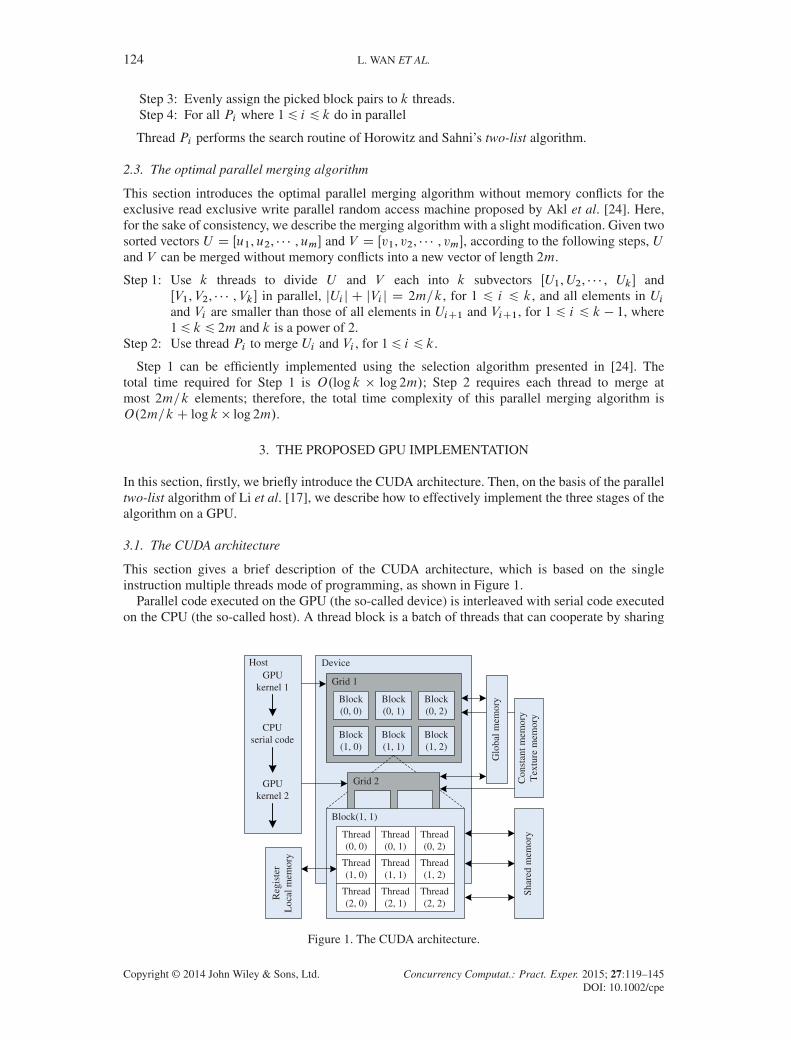
This section gives a brief description of the CUDA architecture, which is based on the singleinstruction multiple threads mode of programming, as shown in Figure 1.
Parallel code executed on the GPU (the so-called device) is interleaved with serial code executedon the CPU (the so-called host). A thread block is a batch of threads that can cooperate by sharing
Figure 1. The CUDA architecture.
Copyright © 2014 John Wiley & Sons, Ltd. Concurrency Computat.: Pract. Exper. 2015; 27:119–145DOI: 10.1002/cpe
GPU IMPLEMENTATION OF A PARALLEL ALGORITHM FOR THE SSP 125
data through shared memory. Threads from different blocks cannot cooperate. These thread blocksare organized into a grid. The basic unit of execution in CUDA is the so-called kernel. When aCUDA program invokes a kernel on the host side, these thread blocks within a grid are enumeratedand distributed to multiprocessors with available execution capacity. All threads within a grid canbe executed in parallel.
As can be seen in Figure 1, the GPU offers multiple memory spaces. Each thread has its own reg-ister and local memory. Each thread block has a shared memory, which is visible to all the threadswithin the same block and has the same lifetime as the block. All threads within a grid can accessthe global memory, the constant memory, and the texture memory. These threads can coordinatememory accesses by synchronizing their executions.
3.2. Task distribution
This section describes how to reasonably assign tasks to CPU and GPU in our GPU implementation.A reasonable task distribution between CPU and GPU is critical for GPU applications, namely,
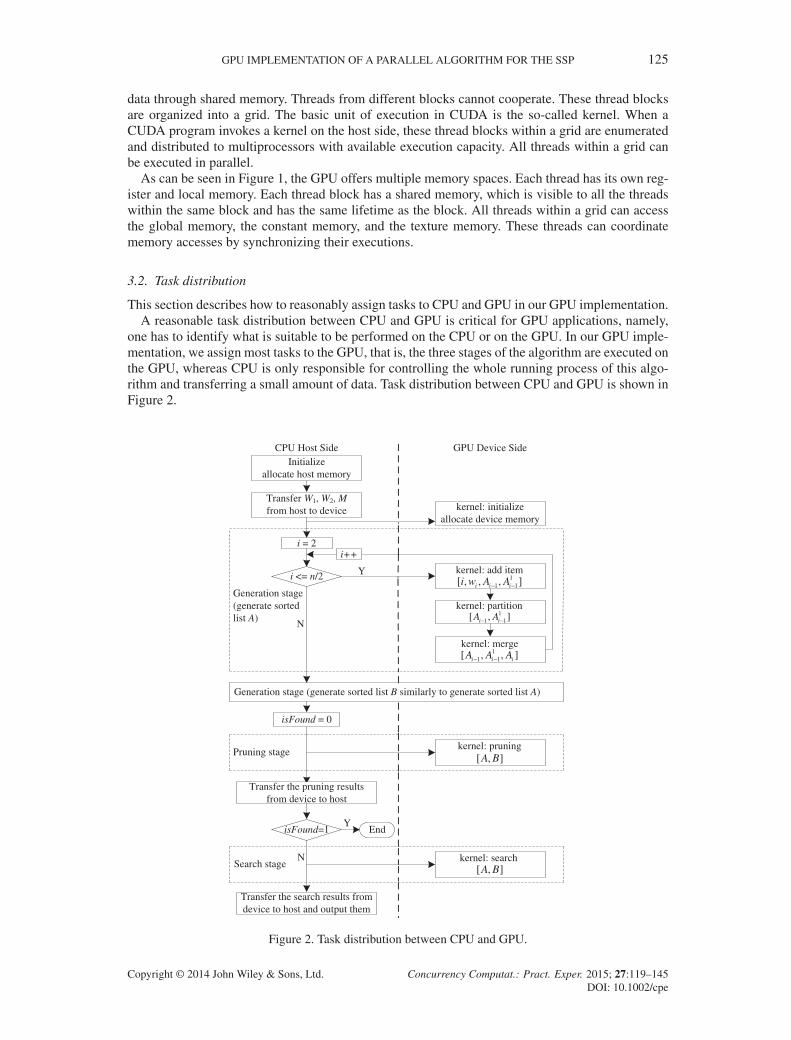
one has to identify what is suitable to be performed on the CPU or on the GPU. In our GPU imple-mentation, we assign most tasks to the GPU, that is, the three stages of the algorithm are executed onthe GPU, whereas CPU is only responsible for controlling the whole running process of this algo-rithm and transferring a small amount of data. Task distribution between CPU and GPU is shown inFigure 2.
Figure 2. Task distribution between CPU and GPU.
Copyright © 2014 John Wiley & Sons, Ltd. Concurrency Computat.: Pract. Exper. 2015; 27:119–145DOI: 10.1002/cpe
126 L. WAN ET AL.
Specifically, our GPU implementation begins with the initialization on the host and device sides.During the host side initialization phase, firstly, we obtain the original n-element input vector W ,divide W into two equal parts W1 and W2, and dynamically allocate host memory and global mem-ory for W1 and W2, where each part contains n=2 items. Secondly, we statically allocate constantmemory for the knapsack capacity M on the device side, and we initialize the capacity value. Fur-thermore, we transfer W1,W2, and M from the host to the device through the system bus. W1 andW2 are stored in the global memory. M is copied to the constant memory, and it can be read by allthe threads in the grid with lower memory access latency than the global memory.
In our GPU implementation, we use the list A to store all of the N subset sums of W1 in non-decreasing order, and we use the list B to store all of the N subset sums of W2 in nonincreasingorder. During the device side initialization phase, we dynamically allocate global memory for listsA and B by executing the initialize kernel, where each list needs O.N/ memory cells. In addition,we initialize A1 D Œ0,w1� and B1 D Œwn=2C1, 0�.
After the initialization phase has completed, we will describe how to execute the three stages ofthe algorithm on a GPU in the following sections.
3.3. The parallel generation stage
This section describes the generation procedure of the nondecreasing list A. The generationprocedure of the nonincreasing list B is almost the same as that of the list A.
Let us suppose that the list A1 D Œ0,w1� has been generated in the previous initializationphase. Firstly, we use k GPU threads to add the item wi to each element of the list Ai�1 DŒai�1.1, ai�1.2, � � � , ai�1.2i�1 � in parallel, generating a new list A1i�1 D Œai�1.1 C wi , ai�1.2 Cwi , � � � , ai�1.2i�1 C wi �, where 2 6 i 6 n=2. Suppose that the maximum number of GPUthreads used is 2n=4. If 2 6 i 6 n=4 C 1, each thread works on one element of the list Ai�1; ifn=4C 1 < i 6 n=2, each thread works on 2i�1=k elements of the list Ai�1. Note that it is neces-sary to load the item wi from global memory to on-chip shared memory, before the add operationis executed by each thread, so as to avoid the high global memory access latency. Then, we mergelists Ai�1 and A1i�1 into a new list Ai with 2i subset sums by using the optimal parallel mergingalgorithm [24], and write Ai into the global memory. By sequentially repeating such steps, aftern=2 � 1 iterations, we finally obtain the list An=2 with N subset sums, that is, the needed sortedlist A.
The basic procedure to generate the nondecreasing list A is described in Algorithm 3, whichshows that the task carried out by the CPU on the host side has three phases: the add item phase,the partition phase, and the merge phase. The three phases correspond to three different kernelscarried out by the GPU on the device side as follows: the add item kernel, the partition kernel, andthe merge kernel. When these kernels are launched on the host side, we must specify the number ofblocks per grid and the number of threads per block (TPB) in gridSize and blockSize, respectively.Between the three phases, we use the function cudaDeviceSynchronize() to synchronize the GPUthreads between two kernel launches, so as to insure data consistency.
From Algorithm 3, it is easy to see that when generating the list Ai , if 2 6 i 6 n=4, the numberof required threads is 2i�1 at most; if n=4 < i 6 n=2, the number of threads used is 2n=4. Hence,we can determine the number of required threads according to the size of the list Ai . Moreover,the communication cost between CPU and GPU can be minimized, because the list A is directlygenerated by executing the three kernels on the GPU, and it is directly stored in the global memory.
3.3.1. The add item phase. In the add item phase, the add item kernel is described in Algorithm 4,which displays the work of a single GPU thread. Here, all k GPU threads can run the kernel inparallel. The tid-th thread adds the item wi to the tid-th element of the list Ai�1, generating thecorresponding tid-th element of the list A1i�1, where 16 t id 6 2i�1.
In Algorithm 4, gridDim.x indicates the number of blocks in a grid in theX -direction; blockDim.xindicates the number of threads in a block in the X -direction; blockIdx.x represents the block indexwithin a grid; and threadIdx.x represents the thread index within a block. In our GPU implementa-tion, we use a one-dimensional block and grid. Thus blockDim.x � gridDim.x is the total number of
Copyright © 2014 John Wiley & Sons, Ltd. Concurrency Computat.: Pract. Exper. 2015; 27:119–145DOI: 10.1002/cpe

GPU IMPLEMENTATION OF A PARALLEL ALGORITHM FOR THE SSP 127
Algorithm 3 The basic procedure to generate the nondecreasing list ARequire: W1 D Œw1,w2, � � � ,wn=2�,A1 D Œ0,w1�
1: for i D 2 to n=2 do2: if 26 i 6 n=4 then3: k D 2i�1;4: else5: k D 2n=4;6: end if7: addItem_kernel<<< gridSi´e, blockSi´e >>>
�i ,wi ,Ai�1,A1i�1
�;
8: cudaDeviceSynchronize();9: for j D 1 to log k do
10: partition_kernel<<< gridSi´e, blockSi´e >>>�j ,Ai�1,A1i�1
�;
11: cudaDeviceSynchronize();12: end for13: merge_kernel<<< gridSi´e, blockSi´e >>>
�Ai�1,A1i�1,Ai
�;
14: cudaDeviceSynchronize();15: end for16: return An=2
Algorithm 4 The add item kernel
Require: i ,wi ,Ai�1,A1i�11: t id D blockIdx.x � blockDim.xC threadIdx.xC 1;2: while t id 6 2i�1 do3: A1i�1Œt id �D Ai�1Œt id �Cwi ;4: t idCD blockDim.x � gridDim.x;5: end while6: return A1i�1
threads running in the grid. Each thread evaluates one copy of the kernel. After each thread accom-plishes its work at the current index tid, if tid is less than or equal to 2i�1, we need to increase tidby blockDim.x � gridDim.x.
3.3.2. The partition phase. The optimal parallel merging algorithm [24] is used in the partition andmerge phases. It is clear that the partition process adopts a typical recursive divide-and-conquerstrategy. However, support for recursion in GPUs with compute capability less than 3.5 is weak.Specifically, they support recursion only for device functions but not for kernel functions, namelythey do not allow a kernel function to call other kernel functions recursively, and thus massive GPUcores cannot be utilized, leading to poor efficiency. As a consequence, we have to develop a newvector-based iterative implementation mechanism instead of the explicit recursion. The partition andmerge phases are illustrated in Figure 3.
As shown in Figure 3, the whole partition process needs to execute log k iterations to complete.In each iteration, the partition kernel is launched from the host side and executed on the device side;the partition kernel is described in Algorithm 5. In the partition phase, the number of required GPUthreads depends on the current iteration number j , where 1 6 j 6 log k. Let threadCounts denotethe number of required GPU threads, which is equal to 2j�1 for the j -th iteration. Note that thecurrent iteration number j should be copied from the host to the device and stored in the on-chipshared memory, before the partition kernel is launched.
In the partition phase, in order to store the partition information (i.e., boundary positions of sub-list) generated by each GPU thread in each iteration, we declare a vector H whose size is 2k � 1.The vectorH is directly defined in the global memory, which can contribute to greatly reducing the
Copyright © 2014 John Wiley & Sons, Ltd. Concurrency Computat.: Pract. Exper. 2015; 27:119–145DOI: 10.1002/cpe

128 L. WAN ET AL.
Figure 3. The partition and merge phases.
Algorithm 5 The partition kernel
Require: j ,Ai�1,A1i�1,H1: t id D blockIdx.x � blockDim.xC threadIdx.xC 1;2: threadCounts D 2j�1;3: while t id 6 threadCounts do4: medianId D t id C threadCounts � 1;5: aDHŒmedianId�.lowA;6: b DHŒmedianId�.highA;7: c DHŒmedianId�.lowB ;8: d DHŒmedianId�.highB ;9: find the median pair (e, f ) of Ai�1Œa, b� and A1i�1Œc, d� by using the selection algorithm;
10: HŒ2 �medianId�.lowA D a;11: HŒ2 �medianId�.highA D e;12: HŒ2 �medianId�.lowB D c;13: HŒ2 �medianId�.highB D f ;14: HŒ2 �medianId C 1�.lowA D eC 1;15: HŒ2 �medianId C 1�.highA D b;16: HŒ2 �medianId C 1�.lowB D f C 1;17: HŒ2 �medianId C 1�.highB D d ;18: t idCD blockDim.x � gridDim.x;19: end while20: return H
communication cost between CPU and GPU, because the partition information does not have to bepassed back and forth to the GPU in each iteration.
Each element of the vector H is a struct with four integer member variables: lowA, highA,lowB and highB . The member variables lowA and highA are used to store the lower bound posi-tion and the upper bound position of sublist X , respectively. Similarly, the member variables lowBand highB are used to store the lower bound position and the upper bound position of sublist Y ,respectively. Before the first iteration, in order to store the boundary positions of lists Ai�1 andA1i�1, we initialize H as follows: HŒ1�.lowA D 1, HŒ1�.highA D 2i�1, HŒ1�.lowB D 1 andHŒ1�.highB D 2i�1.
Here, let Ai�1Œa, b� denote the sublist Œai�1.a, ai�1.aC1, � � � , ai�1.b�, and A1i�1Œc, d� denote thesublist
�a1i�1.c , a
1i�1.cC1, � � � , a1
i�1.d
�, where 2 6 i 6 n=2 and 1 6 a, b, c, d 6 2i�1. The
implementation of partitioning lists Ai�1 and A1i�1 consists of the following log k steps:
Step 1: (j D 1) We only use a single GPU thread P1 to run the partition kernel. At first, P1gets the first element of H . Then, P1 executes the selection algorithm presented in [24]
Copyright © 2014 John Wiley & Sons, Ltd. Concurrency Computat.: Pract. Exper. 2015; 27:119–145DOI: 10.1002/cpe
GPU IMPLEMENTATION OF A PARALLEL ALGORITHM FOR THE SSP 129
to find the median pair .x,y/ of lists Ai�1Œ1, 2i�1� and A1i�1Œ1, 2i�1�. Finally, we usethe second element of H to store the boundary positions .1, x, 1,y/ and use the thirdelement of H to store the boundary positions .xC 1, 2i�1,y C 1, 2i�1/.
Step j : (26 j 6 log k) We use 2j�1 GPU threads to run the partition kernel in parallel. Firstly,the current thread Ptid gets the corresponding element of H via the variable medianId,namely, it gets the corresponding partition information .a, b, c, d/ from the previousiteration, where 1 6 t id 6 2j�1. Secondly, Ptid finds the median pair .e, f / of sublistsAi�1Œa, b� and A1i�1Œc, d�. Finally, the new boundary positions .a, e, c,f / are stored inthe .2 � medianId/-th element of H . In the same way, the new boundary positions.eC 1, b,f C 1, d/ are stored in the .2 �medianId C 1/-th element of H .
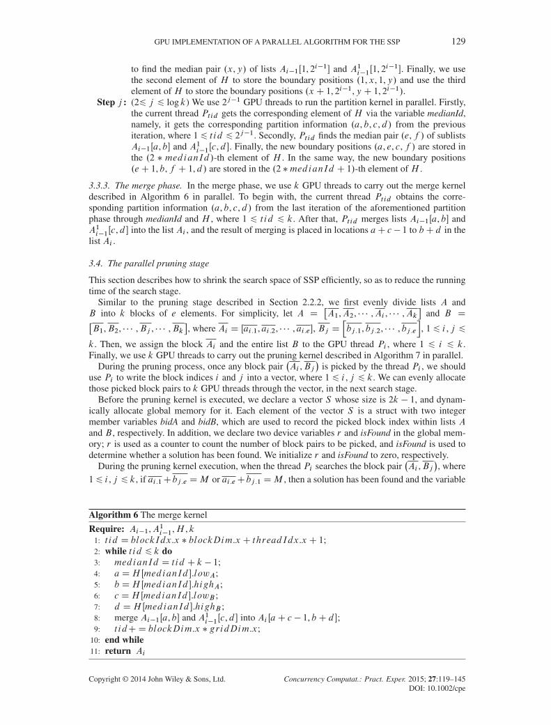
3.3.3. The merge phase. In the merge phase, we use k GPU threads to carry out the merge kerneldescribed in Algorithm 6 in parallel. To begin with, the current thread Ptid obtains the corre-sponding partition information .a, b, c, d/ from the last iteration of the aforementioned partitionphase through medianId and H , where 1 6 t id 6 k. After that, Ptid merges lists Ai�1Œa, b� andA1i�1Œc, d� into the list Ai , and the result of merging is placed in locations aC c � 1 to bC d in thelist Ai .
3.4. The parallel pruning stage
This section describes how to shrink the search space of SSP efficiently, so as to reduce the runningtime of the search stage.
Similar to the pruning stage described in Section 2.2.2, we first evenly divide lists A andB into k blocks of e elements. For simplicity, let A D
�A1,A2, � � � ,Ai , � � � ,Ak
�and B D�
B1,B2, � � � ,Bj , � � � ,Bk�, where Ai D Œai .1, ai .2, � � � , ai .e�, Bj D
hbj .1, bj .2, � � � , bj .e
i, 1 6 i , j 6
k. Then, we assign the block Ai and the entire list B to the GPU thread Pi , where 1 6 i 6 k.Finally, we use k GPU threads to carry out the pruning kernel described in Algorithm 7 in parallel.
During the pruning process, once any block pair�Ai ,Bj
�is picked by the thread Pi , we should
use Pi to write the block indices i and j into a vector, where 1 6 i , j 6 k. We can evenly allocatethose picked block pairs to k GPU threads through the vector, in the next search stage.
Before the pruning kernel is executed, we declare a vector S whose size is 2k � 1, and dynam-ically allocate global memory for it. Each element of the vector S is a struct with two integermember variables bidA and bidB, which are used to record the picked block index within lists Aand B , respectively. In addition, we declare two device variables r and isFound in the global mem-ory; r is used as a counter to count the number of block pairs to be picked, and isFound is used todetermine whether a solution has been found. We initialize r and isFound to zero, respectively.
During the pruning kernel execution, when the thread Pi searches the block pair�Ai ,Bj
�, where
16 i , j 6 k, if ai .1Cbj .e DM or ai .eCbj .1 DM , then a solution has been found and the variable
Algorithm 6 The merge kernel
Require: Ai�1,A1i�1,H , k1: t id D blockIdx.x � blockDim.xC threadIdx.xC 1;2: while t id 6 k do3: medianId D t id C k � 1;4: aDHŒmedianId�.lowA;5: b DHŒmedianId�.highA;6: c DHŒmedianId�.lowB ;7: d DHŒmedianId�.highB ;8: merge Ai�1Œa, b� and A1i�1Œc, d� into Ai ŒaC c � 1, bC d�;9: t idCD blockDim.x � gridDim.x;
10: end while11: return Ai
Copyright © 2014 John Wiley & Sons, Ltd. Concurrency Computat.: Pract. Exper. 2015; 27:119–145DOI: 10.1002/cpe
130 L. WAN ET AL.
isFound is set to 1; if ai .1C bj .e <M and ai .e C bj .1 >M , then the block pair�Ai ,Bj
�is picked,
and the block indices i and j will be stored in the r-th element of S ; otherwise, the block pair�Ai ,Bj
�is directly discarded. Note that isFound and r are global variables, namely they might be
read and changed simultaneously by all k threads. Hence, it is necessary to update them atomically.After the pruning kernel has completed, if isFound=1, we copy the solution from the device to the
host and output it; otherwise, we will carry out the next search stage.
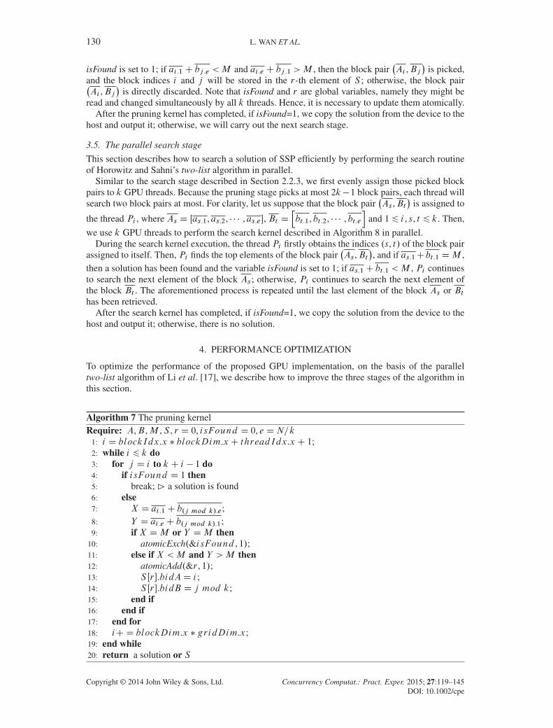
3.5. The parallel search stage
This section describes how to search a solution of SSP efficiently by performing the search routineof Horowitz and Sahni’s two-list algorithm in parallel.
Similar to the search stage described in Section 2.2.3, we first evenly assign those picked blockpairs to k GPU threads. Because the pruning stage picks at most 2k�1 block pairs, each thread willsearch two block pairs at most. For clarity, let us suppose that the block pair
�As ,Bt
�is assigned to
the thread Pi , where As D Œas.1, as.2, � � � , as.e�, Bt Dhbt .1, bt .2, � � � , bt .e
iand 16 i , s, t 6 k. Then,
we use k GPU threads to perform the search kernel described in Algorithm 8 in parallel.During the search kernel execution, the thread Pi firstly obtains the indices .s, t / of the block pair
assigned to itself. Then, Pi finds the top elements of the block pair�As ,Bt
�, and if as.1Cbt .1 DM ,
then a solution has been found and the variable isFound is set to 1; if as.1C bt .1 <M , Pi continuesto search the next element of the block As; otherwise, Pi continues to search the next element ofthe block Bt . The aforementioned process is repeated until the last element of the block As or Bthas been retrieved.
After the search kernel has completed, if isFound=1, we copy the solution from the device to thehost and output it; otherwise, there is no solution.
4. PERFORMANCE OPTIMIZATION
To optimize the performance of the proposed GPU implementation, on the basis of the paralleltwo-list algorithm of Li et al. [17], we describe how to improve the three stages of the algorithm inthis section.
Algorithm 7 The pruning kernelRequire: A,B ,M ,S , r D 0, isFound D 0, e DN=k
1: i D blockIdx.x � blockDim.xC threadIdx.xC 1;2: while i 6 k do3: for j D i to kC i � 1 do4: if isFound D 1 then5: break;B a solution is found6: else7: X D ai .1C b.j mod k/.e;8: Y D ai .e C b.j mod k/.1;9: if X DM or Y DM then
10: atomicExch.&isFound , 1/;11: else if X <M and Y >M then12: atomicAdd.&r , 1/;13: SŒr�.bidAD i ;14: SŒr�.bidB D j mod k;15: end if16: end if17: end for18: iCD blockDim.x � gridDim.x;19: end while20: return a solution or S
Copyright © 2014 John Wiley & Sons, Ltd. Concurrency Computat.: Pract. Exper. 2015; 27:119–145DOI: 10.1002/cpe

GPU IMPLEMENTATION OF A PARALLEL ALGORITHM FOR THE SSP 131
Algorithm 8 The search kernelRequire: A,B ,M ,S , r , isFound , e DN=k
1: i D blockIdx.x � blockDim.xC threadIdx.xC 1;2: while i 6 r do3: s D SŒi �.bidA;4: t D SŒi �.bidB;5: x D 1;6: y D 1;7: while x 6 e and y 6 e do8: if isFound D 1 then9: break;B a solution is found
10: else11: if as.x C bt .y DM then12: atomicExch.&isFound , 1/;13: else if as.x C bt .y <M then14: x D xC 1;15: else16: y D y C 1;17: end if18: end if19: end while20: iCD blockDim.x � gridDim.x;21: end while22: return a solution or NULL
4.1. The improved generation stage
To improve the performance of the generation stage, during the process of generating thenondecreasing list A, we discard those subset sums that exceed the knapsack capacity.
Specifically, we first sort the input vector W in nonincreasing order and then divide it intotwo equal parts W1 and W2. When adding the item wi to each element of the listAi�1 D Œai�1.1, ai�1.2, � � � , ai�1.2i�1 � to generate a new list A1i�1 D Œai�1.1 C wi , ai�1.2 Cwi , � � � , ai�1.2i�1 C wi �, if ai�1.j C wi > M , the subset sum can be directly discarded, namelyit does not need to be stored in the list A1i�1, where 26 i 6 n=2 and 16 j 6 2i�1.
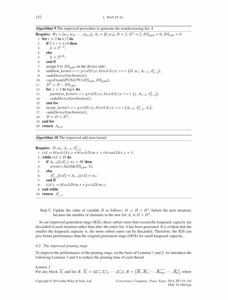
According to this optimization strategy, the improved procedure to generate the nondecreasinglist A is described in Algorithm 9. Let D and D1 denote, respectively, the number of elements tobe processed in the lists Ai�1 and A1i�1, where 2 6 i 6 n=2. Both D and D1 are initialized to 2.Let DSgpu and DScpu denote the number of subset sums to be discarded in the list A1i�1 in eachiteration. Note that DSgpu is a device variable declared in the global memory. The whole processof generating the list A needs to execute n=2 � 1 iterations to complete. Each iteration consists ofthe following five steps:
Step 1: Assign 0 to DSgpu on the device side.Step 2: Use k GPU threads to execute the improved add item kernel described in Algorithm 10 in
parallel. IfAi�1Œt id �Cwi >M , then the subset sum does not need to be stored in the listA1i�1, and the value of variable DSgpu needs to be increased by 1, where 16 t id 6D.
Step 3: Transfer the value of variableDSgpu from the device to the host, and store it into variableDScpu, after completing the add item process.
Step 4: Use k GPU threads to merge Ai�1 and A1i�1 into a new list Ai in parallel. BecauseDScpu subset sums are discarded in the list A1i�1, the number of elements to bemerged in the list A1i�1 is D1 D D �DScpu. Accordingly, during the partition phase,the initial boundary positions of lists Ai�1 and A1i�1 should be updated as follows:HŒ1�.lowA D 1,HŒ1�.highA DD,HŒ1�.lowB D 1,HŒ1�.highB DD1.
Copyright © 2014 John Wiley & Sons, Ltd. Concurrency Computat.: Pract. Exper. 2015; 27:119–145DOI: 10.1002/cpe
132 L. WAN ET AL.
Algorithm 9 The improved procedure to generate the nondecreasing list A
Require: W1 D Œw1,w2, � � � ,wn=2�, A1 D Œ0,w1�, D D 2, D1 D 2, DSgpu D 0, DScpu D 01: for i D 2 to n=2 do2: if 26 i 6 n=4 then3: k D 2i�1;4: else5: k D 2n=4;6: end if7: assign 0 to DSgpu on the device side;8: addItem_kernel<<< gridSi´e, blockSi´e >>>
�D,wi ,Ai�1,A1i�1
�;
9: cudaDeviceSynchronize();10: copyFromGPUToCPU.DScpu,DSgpu/;11: D1 DD �DScpu;12: for j D 1 to log k do13: partition_kernel<<< gridSi´e, blockSi´e >>>
�j ,Ai�1,A1i�1
�;
14: cudaDeviceSynchronize();15: end for16: merge_kernel<<< gridSi´e, blockSi´e >>>
�Ai�1,A1i�1,Ai
�;
17: cudaDeviceSynchronize();18: D DDCD1;19: end for20: return An=2
Algorithm 10 The improved add item kernel
Require: D,wi ,Ai�1,A1i�11: t id D blockIdx.x � blockDim.xC threadIdx.xC 1;2: while t id 6D do3: if Ai�1Œt id �Cwi >M then4: atomicAdd.&DSgpu, 1/;5: else6: A1i�1Œt id �D Ai�1Œt id �Cwi ;7: end if8: t idCD blockDim.x � gridDim.x;9: end while
10: return A1i�1
Step 5: Update the value of variable D as follows: D D D C D1, before the next iteration,because the number of elements in the new list Ai is DCD1.
In our improved generation stage (IGS), those subset sums that exceed the knapsack capacity arediscarded in each iteration rather than after the entire list A has been generated. It is evident that thesmaller the knapsack capacity is, the more subset sums can be discarded. Therefore, the IGS cangive better performance than the original generation stage (OGS) for small knapsack capacity.
4.2. The improved pruning stage
To improve the performance of the pruning stage, on the basis of Lemmas 1 and 2, we introduce thefollowing Lemmas 3 and 4 to reduce the pruning time of each thread.
Lemma 3For any block Ai and list B , Ai D .ai .1, ai .2, � � � , ai .e/, B D
�B1,B2, � � � ,Blow , � � � ,Bk
�, where
Copyright © 2014 John Wiley & Sons, Ltd. Concurrency Computat.: Pract. Exper. 2015; 27:119–145DOI: 10.1002/cpe

GPU IMPLEMENTATION OF A PARALLEL ALGORITHM FOR THE SSP 133
Blow Dhblow .1, blow .2, � � � , blow .e
i, 16 i , low 6 k, if ai .1Cblow�1.e >M and ai .1Cblow .e <M ,
then any block pair�Ai , Bj
�can be discarded, where 1 < low 6 k and 16 j < low.
ProofIt is obvious that the element ai .1 is the smallest element in the block Ai and the element blow�1.e isthe smallest element in the block Blow�1. If the sum of these two elements is greater than M , thenai .1C bj .e >M , where 16 j 6 low � 1. That is, any block pair
�Ai , Bj
�can be discarded. �
Lemma 4For any block Ai and list B , Ai D .ai .1, ai .2, � � � , ai .e/, B D
�B1,B2, � � � ,Bhigh, � � � ,Bk
�,
where Bhigh Dhbhigh.1, bhigh.2, � � � , bhigh.e
i, 1 6 i , high 6 k, if ai .e C bhigh.1 > M and
ai .e C bhighC1.1 < M , then any block pair�Ai , Bj
�can be discarded, where 1 6 high < k
and high < j 6 k.
ProofIt is obvious that the element ai .e is the largest element in the block Ai and the element bhighC1.1 isthe largest element in the block BhighC1. If the sum of these two elements is smaller than M , thenai .e C bj .1 <M , where highC 16 j 6 k. That is, any block pair
�Ai , Bj
�can be discarded. �
On the basis of Lemmas 3 and 4, we use GPU thread Pi to perform two binary searches in thelist B to find the block indices low and high, so as to pick high � low + 1 consecutive blocks Blow ,BlowC1, � � � , Bhigh, which will be associated with block Ai , where 1 6 i 6 k. The improvedpruning kernel is described in Algorithm 11, which consists of the following three steps:
Algorithm 11 The improved pruning kernelRequire: A,B ,M ,S , r D 0, isFound D 0, e DN=k
1: i D blockIdx.x � blockDim.xC threadIdx.xC 1;2: while i 6 k do3: l D 1; r D k;4: while l 6 r and isFound D 0 do5: mD l C .r � l/=2;6: if ai .1C bm.e DM then atomicExch.&isFound , 1/; break;B a solution is found7: else if ai .1C bm.e <M then r Dm� 1; else l DmC 1; end if8: end while9: low D l ; r D k;
10: while l 6 r and isFound D 0 do11: mD l C .r � l/=2;12: if ai .e C bm.1 DM then atomicExch.&isFound , 1/; break;B a solution is found13: else if ai .e C bm.1 >M then l DmC 1; else r Dm� 1; end if14: end while15: highD r ;16: if isFound D 0 then17: for j D low to high do18: atomicAdd.&r , 1/; SŒr�.bidAD i ; SŒr�.bidB D j ;19: end for20: end if21: iCD blockDim.x � gridDim.x;22: end while23: return a solution or S
Copyright © 2014 John Wiley & Sons, Ltd. Concurrency Computat.: Pract. Exper. 2015; 27:119–145DOI: 10.1002/cpe
134 L. WAN ET AL.
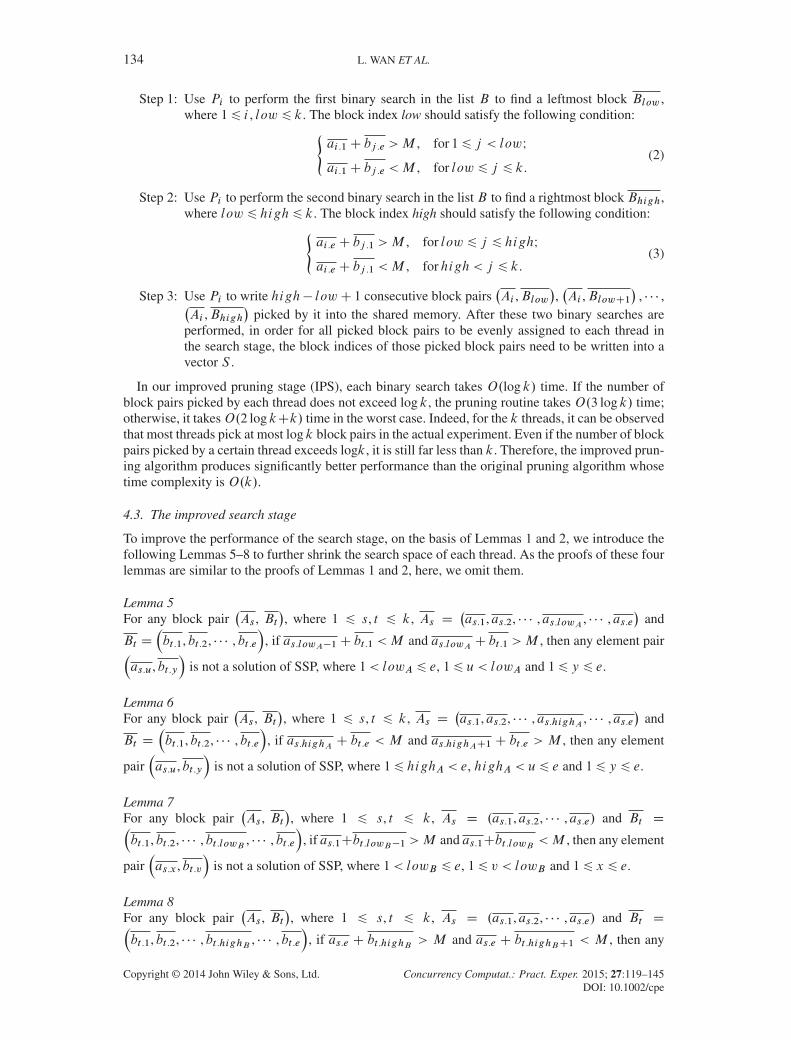
Step 1: Use Pi to perform the first binary search in the list B to find a leftmost block Blow ,where 16 i , low 6 k. The block index low should satisfy the following condition:(
ai .1C bj .e >M , for 16 j < lowIai .1C bj .e <M , for low 6 j 6 k.
(2)
Step 2: Use Pi to perform the second binary search in the list B to find a rightmost block Bhigh,where low 6 high6 k. The block index high should satisfy the following condition:(
ai .e C bj .1 >M , for low 6 j 6 highIai .e C bj .1 <M , forhigh < j 6 k.
(3)
Step 3: Use Pi to write high� lowC 1 consecutive block pairs�Ai ,Blow
�,�Ai ,BlowC1
�, � � � ,�
Ai ,Bhigh�
picked by it into the shared memory. After these two binary searches areperformed, in order for all picked block pairs to be evenly assigned to each thread inthe search stage, the block indices of those picked block pairs need to be written into avector S .
In our improved pruning stage (IPS), each binary search takes O.log k/ time. If the number ofblock pairs picked by each thread does not exceed log k, the pruning routine takes O.3 log k/ time;otherwise, it takesO.2 log kCk/ time in the worst case. Indeed, for the k threads, it can be observedthat most threads pick at most log k block pairs in the actual experiment. Even if the number of blockpairs picked by a certain thread exceeds logk, it is still far less than k. Therefore, the improved prun-ing algorithm produces significantly better performance than the original pruning algorithm whosetime complexity is O.k/.
4.3. The improved search stage
To improve the performance of the search stage, on the basis of Lemmas 1 and 2, we introduce thefollowing Lemmas 5–8 to further shrink the search space of each thread. As the proofs of these fourlemmas are similar to the proofs of Lemmas 1 and 2, here, we omit them.
Lemma 5For any block pair
�As , Bt
�, where 1 6 s, t 6 k, As D
�as.1, as.2, � � � , as.lowA , � � � , as.e
�and
Bt D�bt .1, bt .2, � � � , bt .e
�, if as.lowA�1C bt .1 <M and as.lowA C bt .1 >M , then any element pair�
as.u, bt .y�
is not a solution of SSP, where 1 < lowA 6 e, 16 u < lowA and 16 y 6 e.
Lemma 6For any block pair
�As , Bt
�, where 1 6 s, t 6 k, As D
�as.1, as.2, � � � , as.highA , � � � , as.e
�and
Bt D�bt .1, bt .2, � � � , bt .e
�, if as.highA C bt .e < M and as.highAC1 C bt .e > M , then any element
pair�as.u, bt .y
�is not a solution of SSP, where 16 highA < e, highA < u6 e and 16 y 6 e.
Lemma 7For any block pair
�As , Bt
�, where 1 6 s, t 6 k, As D .as.1, as.2, � � � , as.e/ and Bt D�
bt .1, bt .2, � � � , bt .lowB , � � � , bt .e�
, if as.1Cbt .lowB�1 >M and as.1Cbt .lowB <M , then any element
pair�as.x , bt .v
�is not a solution of SSP, where 1 < lowB 6 e, 16 v < lowB and 16 x 6 e.
Lemma 8For any block pair
�As , Bt
�, where 1 6 s, t 6 k, As D .as.1, as.2, � � � , as.e/ and Bt D�
bt .1, bt .2, � � � , bt .highB , � � � , bt .e�
, if as.e C bt .highB > M and as.e C bt .highBC1 < M , then any
Copyright © 2014 John Wiley & Sons, Ltd. Concurrency Computat.: Pract. Exper. 2015; 27:119–145DOI: 10.1002/cpe

GPU IMPLEMENTATION OF A PARALLEL ALGORITHM FOR THE SSP 135
Algorithm 12 The improved search kernelRequire: A,B ,M ,S , r , isFound D 0, e DN=k
1: i D blockIdx.x � blockDim.xC threadIdx.xC 1;2: while i 6 r do3: s D SŒi �.bidA; t D SŒi �.bidB; lA D 1; rA D e;4: while lA 6 rA and isFound D 0 do5: mD lAC .rA � lA/=2;6: if as.mC bt .1 DM then atomicExch.&isFound , 1/; break;7: else if as.mC bt .1 >M then rA Dm� 1; else lA DmC 1; end if8: end while9: lowA D lA; rA D e;
10: while lA 6 rA and isFound D 0 do11: mD lAC .rA � lA/=2;12: if as.mC bt .e DM then atomicExch.&isFound , 1/; break;13: else if as.mC bt .e <M then lA DmC 1; else rA Dm� 1; end if14: end while15: highA D rA; lB D 1; rB D e;16: while lB 6 rB and isFound D 0 do17: mD lB C .rB � lB/=2;18: if as.lowA C bt .m DM then atomicExch.&isFound , 1/; break;19: else if as.lowA C bt .m <M then rB Dm� 1; else lB DmC 1; end if20: end while21: lowB D lB ; rB D e;22: while lB 6 rB and isFound D 0 do23: mD lB C .rB � lB/=2;24: if as.highA C bt .m DM then atomicExch.&isFound , 1/; break;25: else if as.highA C bt .m >M then lB DmC 1; else rB Dm� 1; end if26: end while27: highB D rB ; x D lowA; y D lowB ;28: while x 6 highA and y 6 highB and isFound D 0 do29: if as.x C bt .y DM then atomicExch.&isFound , 1/; break;B a solution is found30: else if as.x C bt .y <M then x D xC 1; else y D y C 1; end if31: end while32: iCD blockDim.x � gridDim.x;33: end while34: return a solution or NULL
element pair�as.x , bt .v
�is not a solution of SSP, where 1 6 highB < e, highB < v 6 e and
16 x 6 e.
Suppose that the block pair�As ,Bt
�is assigned to the GPU thread Pi , where 1 6 i , s, t 6 k.
On the basis of Lemmas 5 and 6, we use Pi to perform two binary searches in block As to find theelement indices lowA and highA, so as to identify highA � lowA C 1 necessary search elementsas.lowA , as.lowAC1, � � � , as.highA . On the basis of Lemmas 7 and 8, we use Pi to perform two binarysearches in blockBt to find the element indices lowB and highB , so as to identify highB�lowBC1necessary search elements bt .lowB , bt .lowBC1, � � � , bt .highB . The improved search kernel is shownin Algorithm 12, which consists of the following five steps:
Step 1: Use Pi to perform the first binary search in block As to find a leftmost element as.lowA ,where 16 lowA 6 e. The element index lowA should satisfy the following condition:(
as.uC bt .1 <M , for 16 u < lowAIas.uC bt .1 >M , for lowA 6 u6 e.
(4)
Copyright © 2014 John Wiley & Sons, Ltd. Concurrency Computat.: Pract. Exper. 2015; 27:119–145DOI: 10.1002/cpe
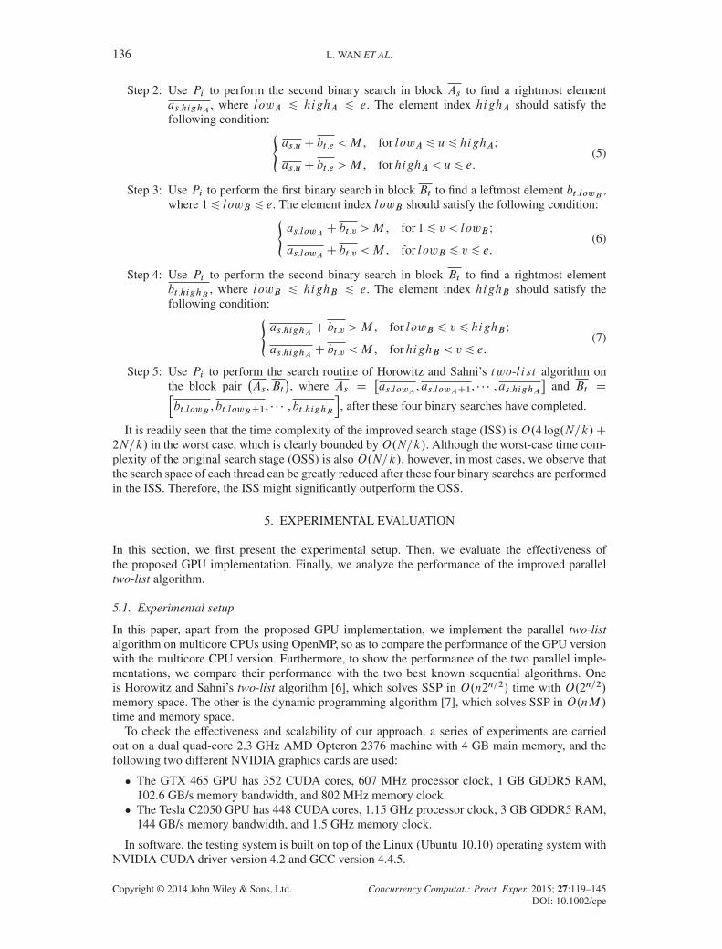
136 L. WAN ET AL.
Step 2: Use Pi to perform the second binary search in block As to find a rightmost elementas.highA , where lowA 6 highA 6 e. The element index highA should satisfy thefollowing condition:(
as.uC bt .e <M , for lowA 6 u6 highAIas.uC bt .e >M , forhighA < u6 e.
(5)
Step 3: Use Pi to perform the first binary search in block Bt to find a leftmost element bt .lowB ,where 16 lowB 6 e. The element index lowB should satisfy the following condition:(
as.lowA C bt .v >M , for 16 v < lowB Ias.lowA C bt .v <M , for lowB 6 v 6 e.
(6)
Step 4: Use Pi to perform the second binary search in block Bt to find a rightmost elementbt .highB , where lowB 6 highB 6 e. The element index highB should satisfy thefollowing condition:(
as.highA C bt .v >M , for lowB 6 v 6 highB Ias.highA C bt .v <M , forhighB < v 6 e.
(7)
Step 5: Use Pi to perform the search routine of Horowitz and Sahni’s two-list algorithm onthe block pair
�As ,Bt
�, where As D
�as.lowA , as.lowAC1, � � � , as.highA
�and Bt Dh
bt .lowB , bt .lowBC1, � � � , bt .highB
i, after these four binary searches have completed.
It is readily seen that the time complexity of the improved search stage (ISS) is O.4 log.N=k/C2N=k/ in the worst case, which is clearly bounded byO.N=k/. Although the worst-case time com-plexity of the original search stage (OSS) is also O.N=k/, however, in most cases, we observe thatthe search space of each thread can be greatly reduced after these four binary searches are performedin the ISS. Therefore, the ISS might significantly outperform the OSS.
5. EXPERIMENTAL EVALUATION
In this section, we first present the experimental setup. Then, we evaluate the effectiveness ofthe proposed GPU implementation. Finally, we analyze the performance of the improved paralleltwo-list algorithm.
5.1. Experimental setup
In this paper, apart from the proposed GPU implementation, we implement the parallel two-listalgorithm on multicore CPUs using OpenMP, so as to compare the performance of the GPU versionwith the multicore CPU version. Furthermore, to show the performance of the two parallel imple-mentations, we compare their performance with the two best known sequential algorithms. Oneis Horowitz and Sahni’s two-list algorithm [6], which solves SSP in O.n2n=2/ time with O.2n=2/memory space. The other is the dynamic programming algorithm [7], which solves SSP in O.nM/
time and memory space.To check the effectiveness and scalability of our approach, a series of experiments are carried
out on a dual quad-core 2.3 GHz AMD Opteron 2376 machine with 4 GB main memory, and thefollowing two different NVIDIA graphics cards are used:
� The GTX 465 GPU has 352 CUDA cores, 607 MHz processor clock, 1 GB GDDR5 RAM,102.6 GB/s memory bandwidth, and 802 MHz memory clock.� The Tesla C2050 GPU has 448 CUDA cores, 1.15 GHz processor clock, 3 GB GDDR5 RAM,
144 GB/s memory bandwidth, and 1.5 GHz memory clock.
In software, the testing system is built on top of the Linux (Ubuntu 10.10) operating system withNVIDIA CUDA driver version 4.2 and GCC version 4.4.5.
Copyright © 2014 John Wiley & Sons, Ltd. Concurrency Computat.: Pract. Exper. 2015; 27:119–145DOI: 10.1002/cpe

GPU IMPLEMENTATION OF A PARALLEL ALGORITHM FOR THE SSP 137
(a) Speedup on the GTX 465 GPU (b) Speedup on the Tesla C2050 GPU
Figure 4. The speedups of GPU implementation on two different GPU cards using six different settings forthreads per block.
We conduct our tests on randomly generated instances of SSP, and we use a random number gen-erator to produce the input vectors W whose sizes range from 36 to 54. They present the followingfeatures:
� wi is randomly drawn in [1, 108], i 2 f1, � � � ,ng.� M D ˛
PniD1wi , ˛ 2 f0.2, � � � , 0.8g.
� wi <M , i 2 f1, � � � ,ng.
In our experiments, we consider the following 10 different problem sizes: 36, 38, 40, 42, 44,46, 48, 50, 52 and 54. Note that the sequential two-list algorithm [6] and the parallel two-listalgorithm [17] all require O.2n=2/ memory space, implying that the problem size will be limitedby the available memory on the testing system. In addition, considering the real-world applica-tions and the worst-case execution time, it is necessary to take into account different knapsackcapacities.
For each problem size, we randomly generate 1000 instances. The average execution time is con-sidered, and the execution time is measured in milliseconds. The speedup is defined as Ts=Tp , whereTs and Tp represent the running time of the sequential implementation and parallel implementation,respectively.
Moreover, to achieve effective and robust performance for the GPU implementation, we shouldadopt the optimum number of TPB to keep the GPU multiprocessors as active as possible. Here,we conduct our preliminary speedup performance tests on the GTX 465 GPU and the Tesla C2050GPU using six different settings for TPB (respectively, 32, 64, 128, 256, 512, and 1024). In thisexperiment, we specify M D 0.5
PniD1wi , and Ts is obtained by executing Horowitz and Sahni’s
sequential two-list algorithm. Note that the maximum number of TPB is 1024 for both cards, thusat most 1024 threads can be specified in each block.
Figure 4 shows the speedups of the GPU implementation on two different GPU cards using sixdifferent settings for TPB. For the 10 different problem sizes, among the six different settings forTPB, Figures 4(a) and 4(b) show that the 128 TPB case seems to be the most efficient. It alwaysgives more stable and scalable speedup, because it can obtain the best multiprocessor occupancy.Hence, we choose the 128 TPB case for further performance tests on both the GTX 465 GPU andTesla C2050 GPU.
5.2. Comparison with CPU implementation
To accurately evaluate the performance of the proposed GPU implementation, for each randomlygenerated instance, we first run the dynamic programming algorithm and Horowitz and Sahni’ssequential two-list algorithm on the CPU. Then, we run the parallel two-list algorithm on multicore
Copyright © 2014 John Wiley & Sons, Ltd. Concurrency Computat.: Pract. Exper. 2015; 27:119–145DOI: 10.1002/cpe

138 L. WAN ET AL.
Table II. Experimental results on the CPU and two different GPU cards.
Sequential algorithm Parallel two-list algorithm
DP two-list Multicore CPUs GTX 465 GPU Tesla C2050 GPUM n Time Time Time Sp-DP Sp-TL Time Sp-DP Sp-TL Time Sp-DP Sp-TL
Case 1
36 27.93 61.29 26.51 1.05 2.31 20.72 1.35 2.96 20.09 1.39 3.0538 53.15 115.24 47.96 1.11 2.40 35.08 1.52 3.29 33.67 1.58 3.4240 110.54 205.45 82.39 1.34 2.49 54.85 2.02 3.75 52.17 2.12 3.9442 230.64 358.29 132.17 1.74 2.71 80.89 2.85 4.43 76.59 3.01 4.6844 480.16 645.12 215.58 2.23 2.99 123.78 3.88 5.21 112.88 4.25 5.72
Case 2
46 2127.87 1151.77 365.69 5.82 3.15 202.50 10.51 5.69 184.17 11.55 6.2548 4183.82 2132.49 650.35 6.43 3.28 353.82 11.82 6.03 321.88 13.00 6.6350 8714.37 4093.46 1217.46 7.16 3.36 652.89 13.35 6.27 593.12 14.69 6.9052 16685.87 7971.76 2234.80 7.47 3.57 1239.60 13.46 6.43 1129.92 14.77 7.0654 33935.49 16124.25 4377.58 7.75 3.68 2490.87 13.62 6.47 2265.74 14.98 7.12
Case 1: M D 0.5PniD1 wi Š
182n=2 Case 2: M D 0.5
PniD1 wi Š
142n=2
DP, dynamic programming; Sp-DP, speedup over the sequential dynamic programming algorithm; Sp-TL, speedupover the sequential two-list algorithm.
CPUs with eight OpenMP threads. Finally, we run the parallel two-list algorithm on two differentGPU cards. Table II shows the execution times of the dynamic programming algorithm and Horowitzand Sahni’s sequential two-list algorithm, and it also shows the execution times and speedups of themulticore CPU implementation and the GPU implementation, respectively, for the 10 different prob-lem sizes. In the experiments, the knapsack capacity M is half the total weight, which is moderatefor the first five problem sizes and is large for the other five problem sizes.
In Table II, it is not hard to see that the dynamic programming technique is attractive for moder-ate knapsack capacity, but Horowitz and Sahni’s two-list algorithm is attractive for large knapsackcapacity. It can be found that when the problem size increases, the execution time and the speedupfactor also increase, and the multicore CPU implementation and the GPU implementation showbetter performance over the two sequential implementations.
The performance comparison between the GPU implementation and the two sequential imple-mentations shows that the speedup is not substantial for small problem sizes (n 6 42). This isassociated with the fact that there may not be enough work to fully utilize the available hardwareparallelism of the GPU. On the other hand, the execution of the GPU program involves some fixedoverheads: thread creation and destruction overhead, GPU initialization overhead, GPU memoryallocation overhead, GPU synchronization overhead, and data transfer overhead. This makes GPUnot suitable for small computational tasks, as these fixed overheads are higher than the kernel exe-cution time. However, for large problem sizes (n > 42), the GPU implementation can achievesubstantial speedup, in comparison with the two sequential implementations, it obtains 14.98 and7.12 speedup, respectively, when n D 54. Hence, the proposed GPU implementation is most fit forlarge-scale SSP.
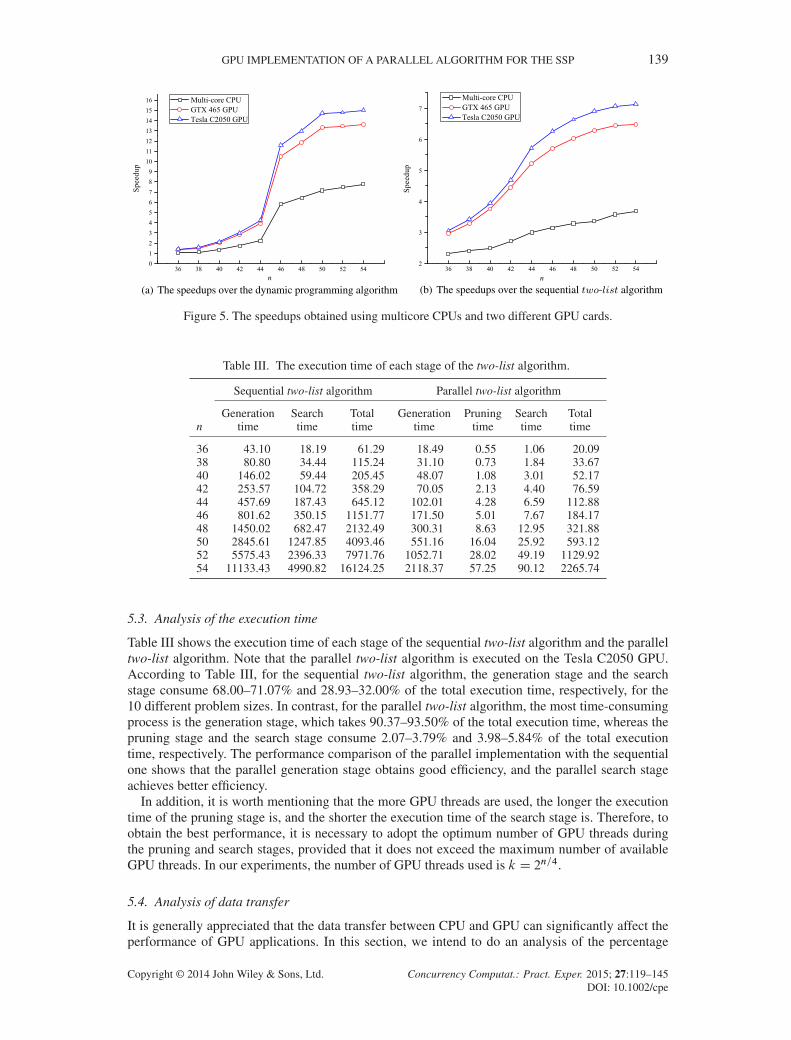
Figures 5(a) and 5(b) illustrate the speedups of the multicore CPU implementation and the GPUimplementation over the dynamic programming algorithm and the sequential two-list algorithm. Aswe can see, as long as the problem size increases, the speedup factor grows accordingly. It is obviousthat the GPU implementation has much better performance than the multicore CPU implementation,because a large number of cores are available on both the GTX 465 GPU and Tesla C2050 GPU.Note that the larger the problem size is, the slower the speedup increases, and the speedup willgradually reach a peak.
The results from Figures 5(a) and 5(b) also show that the GTX 465 GPU and the Tesla C2050GPU offer similar performance for small problem sizes (n 6 42). However, when the problem sizeexceeds 42, the Tesla C2050 GPU yields higher speedup than the GTX 465 GPU. This is due to thefact that the Tesla C2050 GPU enjoys more available streaming processor cores and higher memorybandwidth than the GTX 465 GPU.
Copyright © 2014 John Wiley & Sons, Ltd. Concurrency Computat.: Pract. Exper. 2015; 27:119–145DOI: 10.1002/cpe
GPU IMPLEMENTATION OF A PARALLEL ALGORITHM FOR THE SSP 139
Figure 5. The speedups obtained using multicore CPUs and two different GPU cards.
Table III. The execution time of each stage of the two-list algorithm.
Sequential two-list algorithm Parallel two-list algorithm
Generation Search Total Generation Pruning Search Totaln time time time time time time time
36 43.10 18.19 61.29 18.49 0.55 1.06 20.0938 80.80 34.44 115.24 31.10 0.73 1.84 33.6740 146.02 59.44 205.45 48.07 1.08 3.01 52.1742 253.57 104.72 358.29 70.05 2.13 4.40 76.5944 457.69 187.43 645.12 102.01 4.28 6.59 112.8846 801.62 350.15 1151.77 171.50 5.01 7.67 184.1748 1450.02 682.47 2132.49 300.31 8.63 12.95 321.8850 2845.61 1247.85 4093.46 551.16 16.04 25.92 593.1252 5575.43 2396.33 7971.76 1052.71 28.02 49.19 1129.9254 11133.43 4990.82 16124.25 2118.37 57.25 90.12 2265.74
5.3. Analysis of the execution time
Table III shows the execution time of each stage of the sequential two-list algorithm and the paralleltwo-list algorithm. Note that the parallel two-list algorithm is executed on the Tesla C2050 GPU.According to Table III, for the sequential two-list algorithm, the generation stage and the searchstage consume 68.00–71.07% and 28.93–32.00% of the total execution time, respectively, for the10 different problem sizes. In contrast, for the parallel two-list algorithm, the most time-consumingprocess is the generation stage, which takes 90.37–93.50% of the total execution time, whereas thepruning stage and the search stage consume 2.07–3.79% and 3.98–5.84% of the total executiontime, respectively. The performance comparison of the parallel implementation with the sequentialone shows that the parallel generation stage obtains good efficiency, and the parallel search stageachieves better efficiency.
In addition, it is worth mentioning that the more GPU threads are used, the longer the executiontime of the pruning stage is, and the shorter the execution time of the search stage is. Therefore, toobtain the best performance, it is necessary to adopt the optimum number of GPU threads duringthe pruning and search stages, provided that it does not exceed the maximum number of availableGPU threads. In our experiments, the number of GPU threads used is k D 2n=4.
5.4. Analysis of data transfer
It is generally appreciated that the data transfer between CPU and GPU can significantly affect theperformance of GPU applications. In this section, we intend to do an analysis of the percentage
Copyright © 2014 John Wiley & Sons, Ltd. Concurrency Computat.: Pract. Exper. 2015; 27:119–145DOI: 10.1002/cpe
140 L. WAN ET AL.
0%
10%
20%
30%
40%
50%
60%
70%
80%
90%
100%
36 38 40 42 44 46 48 50 52 54n
Tim
e sp
ent d
urin
g ex
ecut
ion[
%]
Data transferGPU computation
Figure 6. The percentage of the time spent by GPU computation and data transfer.
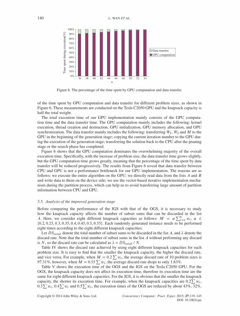
of the time spent by GPU computation and data transfer for different problem sizes, as shown inFigure 6. These measurements are conducted on the Tesla C2050 GPU and the knapsack capacity ishalf the total weight.
The total execution time of our GPU implementation mainly consists of the GPU computa-tion time and the data transfer time. The GPU computation mainly includes the following: kernelexecution, thread creation and destruction, GPU initialization, GPU memory allocation, and GPUsynchronization. The data transfer mainly includes the following: transferringW1,W2 andM to theGPU in the beginning of the generation stage; copying the current iteration number to the GPU dur-ing the execution of the generation stage; transferring the solution back to the CPU after the pruningstage or the search phase has completed.
Figure 6 shows that the GPU computation dominates the overwhelming majority of the overallexecution time. Specifically, with the increase of problem size, the data transfer time grows slightly,but the GPU computation time grows greatly, meaning that the percentage of the time spent by datatransfer will be reduced progressively. The results from Figure 6 reveal that data transfer betweenCPU and GPU is not a performance bottleneck for our GPU implementation. The reasons are asfollows: we execute the entire algorithm on the GPU; we directly read data from the lists A and Band write data to them on the device side; we use the vector-based iterative implementation mecha-nism during the partition process, which can help us to avoid transferring large amount of partitioninformation between CPU and GPU.
5.5. Analysis of the improved generation stage
Before comparing the performance of the IGS with that of the OGS, it is necessary to studyhow the knapsack capacity affects the number of subset sums that can be discarded in the listA. Here, we consider eight different knapsack capacities as follows: M D ˛
PniD1wi , ˛ 2
f0.2, 0.25, 0.3, 0.35, 0.4, 0.45, 0.5, 0.55g. Each randomly generated instance needs to be performedeight times according to the eight different knapsack capacities.
LetDStotal denote the total number of subset sums to be discarded in the list A, and � denote thediscard rate. Note that the total number of subset sums in the list A without performing any discardis N , so the discard rate can be calculated as � = DStotal / N .
Table IV shows the discard rate achieved by using eight different knapsack capacities for eachproblem size. It is easy to find that the smaller the knapsack capacity, the higher the discard rate,and vice versa. For example, when M D 0.2
Pwi , the average discard rate of 10 problem sizes is
97.31%, however, when M D 0.55Pwi , the average discard rate drops to only 1.63%.
Table V shows the execution time of the OGS and the IGS on the Tesla C2050 GPU. For theOGS, the knapsack capacity does not affect its execution time, therefore its execution time are thesame for eight different knapsack capacities. For the IGS, it is obvious that the smaller the knapsackcapacity, the shorter its execution time. For example, when the knapsack capacities are 0.2
Pwi ,
0.3Pwi , 0.4
Pwi and 0.5
Pwi , the execution times of the OGS are reduced by about 43%, 32%,
Copyright © 2014 John Wiley & Sons, Ltd. Concurrency Computat.: Pract. Exper. 2015; 27:119–145DOI: 10.1002/cpe

GPU IMPLEMENTATION OF A PARALLEL ALGORITHM FOR THE SSP 141
Table IV. The discard rate for different knapsack capacities.
����nM
0.2Pwi 0.25
Pwi 0.3
Pwi 0.35
Pwi 0.4
Pwi 0.45
Pwi 0.5
Pwi 0.55
Pwi
36 0.9722 0.9213 0.8124 0.6057 0.3722 0.1818 0.0731 0.016038 0.9755 0.9232 0.8110 0.6061 0.3749 0.1858 0.0729 0.015940 0.9719 0.9231 0.8111 0.6072 0.3728 0.1840 0.0712 0.016242 0.9709 0.9203 0.8132 0.6010 0.3758 0.1858 0.0716 0.016344 0.9733 0.9226 0.8107 0.6079 0.3714 0.1869 0.0726 0.016146 0.9750 0.9215 0.8113 0.6046 0.3702 0.1826 0.0743 0.016448 0.9768 0.9253 0.8103 0.6037 0.3732 0.1802 0.0728 0.016350 0.9719 0.9205 0.8143 0.6054 0.3747 0.1866 0.0733 0.016852 0.9728 0.9225 0.8139 0.6078 0.3711 0.1851 0.0729 0.016154 0.9710 0.9235 0.8102 0.6081 0.3706 0.1833 0.0744 0.0167
Average 0.9731 0.9224 0.8118 0.6057 0.3727 0.1842 0.0729 0.0163
Table V. Execution time comparison between IGS and OGS on the Tesla C2050 GPU.
IGS
n OGS 0.2Pwi 0.25
Pwi 0.3
Pwi 0.35
Pwi 0.4
Pwi 0.45
Pwi 0.5
Pwi 0.55
Pwi
36 18.49 10.57 11.52 12.65 13.92 15.84 17.34 18.14 18.3938 31.10 17.79 19.38 21.27 23.42 26.65 29.17 30.51 30.9540 48.07 27.50 29.95 32.88 36.20 41.19 45.09 47.16 47.8342 70.05 40.07 43.64 47.92 52.75 60.04 65.71 68.72 69.7044 102.01 58.35 63.55 69.77 76.81 87.42 95.68 100.07 101.5046 171.50 98.10 106.84 117.30 129.14 146.97 160.87 168.24 170.6448 300.31 171.78 187.09 205.41 226.13 257.36 281.69 294.60 298.8150 551.16 315.26 343.37 376.99 415.02 472.34 516.99 540.69 548.4052 1052.71 602.15 655.84 720.05 792.69 902.17 987.44 1032.71 1047.4454 2118.37 1211.71 1319.74 1448.96 1595.13 1815.44 1987.03 2078.12 2107.78
IGS, improved generation stage; OGS, original generation stage.
14% and 2%, respectively, for each problem size. The execution time comparison between IGS andOGS shows that our IGS yields significant performance benefits when M < 0.5
Pwi .
5.6. Analysis of the improved pruning stage
Because the number of block pairs picked by each GPU thread can affect the performance of theIPS, this section first shows the excess rate and then presents a performance comparison betweenthe IPS and the original pruning stage (OPS).
Let EXtotal denote the total number of the threads, which pick more than log k block pairs, and� denote the excess rate. Note that the total number of threads used in the IPS is k, the excess ratecan be calculated as � DEXtotal=k.
Table VI shows the excess rate achieved by using seven different knapsack capacities for eachproblem size. We can easily see that most threads pick less than log k block pairs, especially whenM D 0.5
Pwi , almost all threads pick less than log k block pairs. The results from VI reveal that
our IPS should be able to achieve better performance.Table VII shows the execution time of the OPS and the IPS on the Tesla C2050 GPU for
M D 0.5Pwi . It is obvious that our IPS achieves significantly better performance than the OPS.
For example, when the problem sizes are 36, 42, 48, and 54, the execution times of the OPS arereduced by 80%, 84.98%, 88.53%, and 91.41%, respectively.
5.7. Analysis of the improved search stage
Because the performance of the OSS is improved by reducing the search spaces of those pickedblock pairs, this section first shows the search space reduction rate and then presents a performancecomparison between the ISS and the OSS.
Copyright © 2014 John Wiley & Sons, Ltd. Concurrency Computat.: Pract. Exper. 2015; 27:119–145DOI: 10.1002/cpe

142 L. WAN ET AL.
Table VI. The excess rate for different knapsack capacities.
����nM
0.2Pwi 0.3
Pwi 0.4
Pwi 0.5
Pwi 0.6
Pwi 0.7
Pwi 0.8
Pwi
36 0.0031 0.0141 0.0154 0.0002 0.0155 0.0142 0.003238 0.0025 0.0136 0.0149 0.0001 0.0150 0.0137 0.002640 0.0021 0.0116 0.0136 0.0001 0.0137 0.0115 0.002142 0.0019 0.0113 0.0133 0.0000 0.0134 0.0112 0.001844 0.0016 0.0110 0.0131 0.0000 0.0131 0.0110 0.001546 0.0014 0.0098 0.0129 0.0000 0.0130 0.0098 0.001348 0.0012 0.0096 0.0126 0.0000 0.0127 0.0095 0.001150 0.0010 0.0094 0.0123 0.0000 0.0124 0.0093 0.001052 0.0009 0.0092 0.0120 0.0000 0.0121 0.0091 0.000854 0.0008 0.0090 0.0117 0.0000 0.0118 0.0089 0.0007
Average 0.0017 0.0109 0.0132 0.0000 0.0133 0.0108 0.0016
Table VII. Execution time comparison between IPS and OPS for M D 0.5Pwi .
nD 36 nD 38 nD 40 nD 42 nD 44 nD 46 nD 48 nD 50 nD 52 nD 54
OPS 0.55 0.73 1.08 2.13 4.28 5.01 8.63 16.04 28.02 57.25IPS 0.11 0.14 0.17 0.32 0.59 0.65 0.99 1.72 2.67 4.92
OPS, original pruning stage; IPS, improved pruning stage.
Table VIII. The search space reduction rate for different knapsack capacities.
0.3Pwi 0.4
Pwi 0.5
Pwi 0.6
Pwi 0.7
Pwi
n A B A B A B A B A B
36 0.4430 0.5119 0.4554 0.4966 0.4522 0.4999 0.4563 0.4973 0.4429 0.510238 0.4342 0.5160 0.4520 0.4988 0.4515 0.5082 0.4543 0.4989 0.4335 0.519140 0.4353 0.5108 0.4572 0.4956 0.4518 0.5015 0.4572 0.4996 0.4448 0.518342 0.4419 0.5103 0.4596 0.4977 0.4521 0.4954 0.4562 0.4982 0.4509 0.515544 0.4443 0.5173 0.4580 0.4981 0.4512 0.5016 0.4577 0.4968 0.4436 0.518246 0.4563 0.5173 0.4568 0.4951 0.4515 0.5015 0.4542 0.4992 0.4559 0.519148 0.4398 0.5198 0.4567 0.4997 0.4516 0.5013 0.4567 0.4996 0.4394 0.512450 0.4393 0.5190 0.4571 0.4953 0.4517 0.5016 0.4571 0.4953 0.4393 0.519052 0.4405 0.5153 0.4564 0.4951 0.4519 0.5052 0.4564 0.4961 0.4341 0.513954 0.4418 0.5156 0.4570 0.4970 0.4520 0.5024 0.4565 0.4945 0.4419 0.5175
Average 0.4416 0.5153 0.4566 0.4969 0.4517 0.5019 0.4562 0.4976 0.4426 0.5163
Suppose that the block pair�As ,Bt
�is assigned to the thread Pi , where 1 6 i , s, t 6 k. For the
OSS, the search space of block As ranges from as.1 to as.e , and the search space of block Bt rangesfrom bt .1 to bt .e . For the ISS, the search space of block As ranges from as.lowA to as.highA , andthe search space of block Bt ranges from bt .lowB to bt .highB . Therefore, the search space reductionrates of block As and block Bt are .e� .highA� lowAC 1//=e and .e� .highB � lowB C 1//=e,respectively.
Table VIII shows the average search space reduction rate of all picked block pairs achieved byusing five different knapsack capacities for each problem size. Columns ‘A’ and ‘B’ represent theaverage search space reduction rate of these blocks from lists A and B in all picked block pairs,respectively. It is clear that the search space of each picked block pair is greatly reduced; the searchspace reduction rate of one block from lists A and B in each picked block pair are around 45% and50%, respectively.
Copyright © 2014 John Wiley & Sons, Ltd. Concurrency Computat.: Pract. Exper. 2015; 27:119–145DOI: 10.1002/cpe
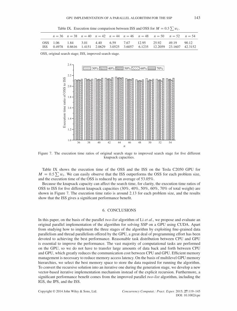
GPU IMPLEMENTATION OF A PARALLEL ALGORITHM FOR THE SSP 143
Table IX. Execution time comparison between ISS and OSS for M D 0.5Pwi .
nD 36 nD 38 nD 40 nD 42 nD 44 nD 46 nD 48 nD 50 nD 52 nD 54
OSS 1.06 1.84 3.01 4.40 6.59 7.67 12.95 25.92 49.19 90.12ISS 0.4978 0.8616 1.4151 2.0629 3.0525 3.6057 6.1235 12.2059 23.1607 42.3152
OSS, original search stage; ISS, improved search stage.
Figure 7. The execution time ratios of original search stage to improved search stage for five differentknapsack capacities.
Table IX shows the execution time of the OSS and the ISS on the Tesla C2050 GPU forM D 0.5
Pwi . We can easily observe that the ISS outperforms the OSS for each problem size,
and the execution time of the OSS is reduced by an average of 53.05%.Because the knapsack capacity can affect the search time, for clarity, the execution time ratios of
OSS to ISS for five different knapsack capacities (30%, 40%, 50%, 60%, 70% of total weight) areshown in Figure 7. The execution time ratio is around 2.13 for each problem size, and the resultsshow that the ISS gives a significant performance benefit.
6. CONCLUSIONS
In this paper, on the basis of the parallel two-list algorithm of Li et al., we propose and evaluate anoriginal parallel implementation of the algorithm for solving SSP on a GPU using CUDA. Apartfrom studying how to implement the three stages of the algorithm by exploiting fine-grained dataparallelism and thread parallelism offered by the GPU, a great deal of programming effort has beendevoted to achieving the best performance. Reasonable task distribution between CPU and GPUis essential to improve the performance. The vast majority of computational tasks are performedon the GPU, so we do not have to transfer large amounts of data back and forth between CPUand GPU, which greatly reduces the communication cost between CPU and GPU. Efficient memorymanagement is necessary to reduce memory access latency. On the basis of multilevel GPU memoryhierarchies, we select the best memory space to store the data required for running the algorithm.To convert the recursive solution into an iterative one during the generation stage, we develop a newvector-based iterative implementation mechanism instead of the explicit recursion. Furthermore, asignificant performance benefit comes from the improved parallel two-list algorithm, including theIGS, the IPS, and the ISS.
Copyright © 2014 John Wiley & Sons, Ltd. Concurrency Computat.: Pract. Exper. 2015; 27:119–145DOI: 10.1002/cpe

144 L. WAN ET AL.
A series of experiments are conducted to test the performance of our GPU implementation underdifferent experimental environments. The experimental results show that the GPU implementationhas much better performance than the CPU implementation and can achieve significant speedupon different GPU cards. The experimental results also show that the improved algorithm can bringsignificant performance benefits for our GPU implementation.
From a hardware point of view, the major consideration for our GPU implementation is the mem-ory available on the GPU. Up to now, the largest single GPU memory space available does notexceed 8 GB, which is far from meeting the memory requirements for large-scale SSP. In futurework, we will explore new techniques to solve large-scale SSP on heterogeneous CPU/GPU clustersystems with less communication overhead and optimal load balancing.
ACKNOWLEDGEMENTS
The authors would like to thank the editor and anonymous reviewers for their valuable suggestions whichconsiderably helped us to enhance this paper. This work was partially funded by the Key Program of NationalNatural Science Foundation of China (Grant No. 61133005), and the National Natural Science Foundationof China (Grant Nos. 61070057, 61370095, 61173013, 61370098)NSFC61070057, 61370095, 61173013, 61370098Key Program of NSFC61133005
REFERENCES
1. Gary MR, Johnson DS. Computers and Intractability: A Guide to the Theory of NP-Completeness. WH Freeman andCompany: New York, 1979.
2. Dietrich BL, Escudero LF, Chance F. Efficient reformulation for 0–1 programs–methods and computational results.Discrete Applied Mathematics 1993; 42(2):147–175.
3. Dyckhoff H. A new linear programming approach to the cutting stock problem. Operations Research 1981;29(6):1092–1104.
4. Kleywegt AJ, Papastavrou JD. The dynamic and stochastic knapsack problem with random sized items. OperationsResearch 2001; 49(1):26–41.
5. Martello S, Toth P. Knapsack Problems: Algorithms and Computer Implementations. John Wiley & Sons, Inc.: NewYork, NY, 1990.
6. Horowitz E, Sahni S. Computing partitions with applications to the knapsack problem. Journal of the ACM (JACM)1974; 21(2):277–292.
7. Bellman RE. Dynamic Programming. Princeton University Press: Princeton, New Jersey, 1957.8. Schroeppel R, Shamir A. A T=O.2n=2), S=O.2n=4) algorithm for certain NP-complete problems. SIAM Journal on
Computing 1981; 10(3):456–464.9. Karnin ED. A parallel algorithm for the knapsack problem. IEEE Transactions on Computers 1984; 100(5):404–408.10. Ferreira AG. A parallel time/hardware tradeoff T �H DO.2n=2/ for the knapsack problem. IEEE Transactions on
Computers 1991; 40(2):221–225.11. Chang HKC, Chen JJR, Shyu SJ. A parallel algorithm for the knapsack problem using a generation and searching
technique. Parallel Computing 1994; 20(2):233–243.12. Lou DC, Chang CC. A parallel two-list algorithm for the knapsack problem. Parallel Computing 1997;
22(14):1985–1996.13. Sanches CAA, Soma NY, Yanasse HH. Comments on parallel algorithms for the knapsack problem. Parallel
Computing 2002; 28(10):1501–1505.14. Sanches CAA, Soma NY, Yanasse HH. An optimal and scalable parallelization of the two-list algorithm for the
subset-sum problem. European Journal of Operational Research 2007; 176(2):870–879.15. Chedid FB. An optimal parallelization of the two-list algorithm of cost O.2n=2/. Parallel Computing 2008;
34(1):63–65.16. Chedid FB. A note on developing optimal and scalable parallel two-list algorithms. In Algorithms and Architectures
for Parallel Processing. Springer-Verlag: Berlin, 2012; 148–155.17. Li KL, Li RF, Li QH. Optimal parallel algorithms for the knapsack problem without memory conflicts. Journal of
Computer Science and Technology 2004; 19(6):760–768.18. Ryoo S, Rodrigues CI, Stone SS, Stratton JA, Ueng SZ, Baghsorkhi SS, Hwu WmW. Program optimization carving
for GPU computing. Journal of Parallel and Distributed Computing 2008; 68(10):1389–1401.19. Che S, Boyer M, Meng J, Tarjan D, Sheaffer JW, Skadron K. A performance study of general-purpose applications
on graphics processors using CUDA. Journal of Parallel and Distributed Computing 2008; 68(10):1370–1380.20. Bokhari SS. Parallel solution of the subset-sum problem: an empirical study. Concurrency and Computation:
Practice & Experience 2012; 24(18):2241–2254.
Copyright © 2014 John Wiley & Sons, Ltd. Concurrency Computat.: Pract. Exper. 2015; 27:119–145DOI: 10.1002/cpe
GPU IMPLEMENTATION OF A PARALLEL ALGORITHM FOR THE SSP 145
21. Boyer V, El Baz D, Elkihel M. Solving knapsack problems on GPU. Computers & Operations Research 2012;39(1):42–47.
22. Lalami ME, El-Baz D. GPU implementation of the Branch and Bound method for knapsack problems. 2012IEEE 26th International Parallel and Distributed Processing Symposium Workshops & PhD Forum (IPDPSW), IEEE,Shanghai, China, 2012; 1769–1777.
23. Pospíchal P, Schwarz J, Jaros J. Parallel genetic algorithm solving 0/1 knapsack problem running on the gpu. 16thInternational Conference on Soft Computing MENDEL, Brno, Czech Republic, 2010; 64–70.
24. Akl SG, Santoro N. Optimal parallel merging and sorting without memory conflicts. IEEE Transactions onComputers 1987; 100(11):1367–1369.
Copyright © 2014 John Wiley & Sons, Ltd. Concurrency Computat.: Pract. Exper. 2015; 27:119–145DOI: 10.1002/cpe