gpu computing for machine learning algorithms -...
TRANSCRIPT

Facoltà di Ingegneria Corso di Studi in Ingegneria Informatica
tesi di laurea
GPU Computing for Machine Learning
Algorithms
Anno Accademico 2010/2011
relatori Ch.mo prof. G. Ventre Ch.mo prof. A. Pescapè correlatore dott. M. Brescia candidato Mauro Garofalo matr. 041/002780

GPU Computing for Machine Learning Algorithms
2
Alla mia famiglia…

GPU Computing for Machine Learning Algorithms
3
Index
1 INTRODUCTION ...................................................................................................................................... 8
2 DATA MINING ON MASSIVE DATA SETS: AN OVERVIEW ........................................................................13
2.1 A SCIENTIFIC USE CASE: ASTROINFORMATICS ..................................................................................................... 17
3 STATE OF THE ART OF COMPUTING TECHNOLOGY ................................................................................23
3.1 GRID COMPUTING ....................................................................................................................................... 24
3.2 CLOUD COMPUTING ................................................................................................................................... 27
3.3 HIGH-PERFORMANCE COMPUTING (HPC) ........................................................................................................ 30
3.4 GPGPU ..................................................................................................................................................... 32
3.5 A DISCUSSION ABOUT COMPUTING ARCHITECTURES............................................................................................. 33
3.6 PARALLEL PROGRAMMING ENVIRONMENT ......................................................................................................... 43
3.6.1 Conventional programming environment: MPI and OpenMP ....................................................... 43
3.7 GPGPU ENVIRONMENT: CUDA ..................................................................................................................... 45
3.7.1 CUDA architecture ......................................................................................................................... 45
3.7.2 Memory Hierarchy ......................................................................................................................... 48
3.7.3 Thread Hierarchy ........................................................................................................................... 49
3.7.4 CUDA C Parallel Programming Model ........................................................................................... 50
3.7.5 CUDA Program Structure ............................................................................................................... 52
3.7.6 Other GPGPU environment: OpenCL .............................................................................................. 53
4 TECHNOLOGY IN MACHINE LEARNING ...................................................................................................57
4.1 THE LEARNING PARADIGMS ............................................................................................................................ 60
4.2 WHAT WE ARE LOOKING FOR IN THE DATA ......................................................................................................... 64
4.3 LEARNING STRATEGIES .................................................................................................................................. 75
4.4 THE NEW GENERATION OF DATA MINING INFRASTRUCTURES ................................................................................. 89

GPU Computing for Machine Learning Algorithms
4
4.5 SELECTED STRATEGY...................................................................................................................................... 94
4.5.1 Data Quality Enhancement with data mining ............................................................................... 96
4.5.2 Data Quality Mining and scalability issues .................................................................................. 100
5 GENETIC ALGORITHMS WITHIN CUDA PARALLEL ARCHITECTURE ........................................................ 104
5.1 GPU DESIGN MODEL ................................................................................................................................. 110
5.1.1 Assess ........................................................................................................................................... 111
5.1.2 Parallelize .................................................................................................................................... 111
5.1.3 Optimize ....................................................................................................................................... 113
5.1.4 Deploy .......................................................................................................................................... 114
5.2 MULTI-CORE DESIGN DESCRIPTION................................................................................................................ 115
5.2.1 Input Files..................................................................................................................................... 126
5.2.2 Input Dataset ............................................................................................................................... 126
5.2.3 Specific use case (training/test/run) configuration file ............................................................... 127
5.2.4 Use case (train/test/run/full) configuration file .......................................................................... 130
5.2.5 Output Files .................................................................................................................................. 131
5.3 PARALLEL REQUIREMENT ANALYSIS ............................................................................................................... 133
5.4 GPU-BASED DEVELOPMENT DESCRIPTION ...................................................................................................... 135
5.4.1 Assess ........................................................................................................................................... 135
5.4.2 Parallelize .................................................................................................................................... 137
5.4.3 Optimize ....................................................................................................................................... 139
5.4.4 Deploy .......................................................................................................................................... 143
6 TEST RESULTS AND PERFORMANCES ................................................................................................... 144
6.1 METRICS DEFINITION .................................................................................................................................. 144
6.2 COMPARISON BETWEEN MULTI-CORE AND GPU ARCHITECTURES ........................................................................ 144
6.3 CLASSIFICATION TEST .................................................................................................................................. 145
6.3.1 Results.......................................................................................................................................... 149

GPU Computing for Machine Learning Algorithms
5
6.4 REGRESSION TEST ....................................................................................................................................... 152
6.4.1 Results.......................................................................................................................................... 153
7 CONCLUSIONS AND FUTURE DEVELOPMENTS ..................................................................................... 154
7.1 CONCLUSIONS ........................................................................................................................................... 154
7.2 FUTURE WORK .......................................................................................................................................... 155
8 ACKNOWLEDGMENTS .......................................................................................................................... 157
9 REFERENCES......................................................................................................................................... 158

GPU Computing for Machine Learning Algorithms
6
Index of Figures
Figure 1 - Cluster-Grid-Cloud computing overview and comparison ....................... 23
Figure 2 – Example of GRID architecture ................................................................. 24
Figure 3 – Example of CLOUD architecture ............................................................. 27
Figure 4 – Example of HPC architecture ................................................................... 30
Figure 5 – The Moore’s CPU Law ............................................................................. 34
Figure 6 – CPU vs. GPU throughput evolution ......................................................... 38
Figure 7 – CPUs and GPUs different design philosophies. ....................................... 39
Figure 8 - CUDA GPU Architecture .......................................................................... 46
Figure 9 - Overview of the CUDA memory model.................................................... 48
Figure 10 - CUDA thread organization ...................................................................... 49
Figure 11 – CUDA with different multi-core architectures ....................................... 51
Figure 12 - CUDA program structure ........................................................................ 53
Figure 13 – A workflow based on supervised learning paradigm .............................. 60
Figure 14 – A workflow based on unsupervised learning paradigm .......................... 63
Figure 15 – correct (a) and wrong (b) separation of classes made by a Perceptron ... 80
Figure 16 – Regions recognized by a MLP with 0, 1, 2 hidden layers ...................... 81
Figure 17 – Classical topology of a MLP with hidden neurons in white circles ....... 81
Figure 18 – typical behavior of error function during learning process ..................... 83
Figure 19 – The variation of weights on different error functions ............................. 83
Figure 20 – Parameter space separated by hyperplanes through SVM model ........... 86
Figure 21 – GPU CUDA memory handling architecture ......................................... 101
Figure 22 – Genetic Algorithms in the hierarchical search method taxonomy ........ 104

GPU Computing for Machine Learning Algorithms
7
Figure 23 - APOD .................................................................................................... 110
Figure 24 – GAME serial (multi-core) version class diagram ................................. 116
Figure 25 – Schematic block diagram for the execution flow of a GA .................... 119
Figure 26 – Roulette selection technique ................................................................. 124
Figure 27- GA flow parallel specializations............................................................. 134
Figure 28 - Visual Profiler discover a Hotspot......................................................... 136
Figure 29 - polyTrigo instructions profile .......................................................... 137
Figure 30 – The field of view (FOV) covered by the 3x3 HST/ACS mosaic in the
F606W band. The central field, with a different orientation, shows the region
covered by previous archival ACS observations in g and z bands. .......................... 147
Figure 31 – Execution time comparison with degree=1........................................... 149
Figure 32 – Execution Time comparison with degree=2 ......................................... 149
Figure 33 - Execution Time comparison with degree=4 .......................................... 150
Figure 34 - Execution Time comparison with degree=8 .......................................... 150
Figure 35 - Speedup comparison .............................................................................. 151

GPU Computing for Machine Learning Algorithms
8
1 Introduction
Computing has rapidly established itself as essential and important to many
branches of science, to the point where computational science is a commonly used
term. Indeed, the application and importance of computing is set to grow
dramatically across almost all the sciences. Computing has started to change how
science is done, enabling new scientific advances through enabling new kinds of
experiments. These experiments are also generating new kinds of data of
increasingly exponential complexity and volume. Achieving the goal of being able
to use, exploit and share these data most effectively is a huge challenge.
It is necessary to merge the capabilities of a file system to store and transmit bulk
data from experiments, with logical organization of files into indexed data
collections, allowing efficient query and analytical operations. It is also necessary to
incorporate extensive metadata describing each experiment and the produced data.

GPU Computing for Machine Learning Algorithms
9
Rather than flat files traditionally used in scientific data processing, the full power of
relational databases is needed to allow effective interactions with the data, and an
interface which can be exploited by the extensive scientific toolkits available, for
purposes such as visualization and plotting.
Different disciplines require support for much more diverse types of tasks than we
find in the large, very coherent and stable virtual organizations. Astronomy, for
example, has far more emphasis on the collation of federated data sets held at
disparate sites (Brescia et al. 2010). There is less massive computation, and large-
scale modeling is generally done on departmental High Performance Computing
(HPC) facilities, where some communities are formed of very small teams and
relatively undeveloped computational infrastructure. In other cases, such as the life
sciences, the problems are far more related to heterogeneous, dispersed data rather
than computation. The harder problem for the future is heterogeneity, of platforms,
data and applications, rather than simply the scale of the deployed resources. The
goal should be to allow scientists to explore the data easily, with sufficient
processing power for any desired algorithm to process it. Current platforms require
the scientists to overcome computing barriers between them and the data (Fabbiano
et al. 2010).
Our convincement is that most aspects of computing will see exponential growth in
bandwidth, but sub-linear or no improvements at all in latency. Moore’s Law will
continue to deliver exponential increases in memory size but the speed with which
data can be transferred between memory and CPUs will remain more or less
constant and marginal improvements can only be made through advances in caching

GPU Computing for Machine Learning Algorithms
10
technology. Certainly Moore’s law will allow the creation of parallel computing
capabilities on single chips by packing multiple CPU cores onto it, but the clock
speed that determines the speed of computation is constrained to remain limited by a
thermal wall (Sutter 2005). We will continue to see exponential growth in disk
capacity, but the factors which determine latency of data transfer will grow sub-
linearly at best, or more likely remain constant. Thus computing machines will not
get much faster. But they will have the parallel computing power and storage
capacity that we used to only get from specialist hardware. As a result, smaller
numbers of supercomputers will be built but at even higher cost. From an
application development point of view, this will require a fundamental paradigm
shift from the currently sequential or parallel programming approach in scientific
applications to a mix of parallel and distributed programming that builds programs
that exploit low latency in multi core CPUs. But they are explicitly designed to cope
with high latency whenever the task at hand requires more computational resources
than can be provided by a single machine. Computing machines can be networked
into clouds or grids of clusters and perform tasks that were traditionally restricted to
supercomputers at a fraction of the cost. A consequence of building grids over wide-
area networks and across organizational boundaries is that the currently prevailing
synchronous approach to distributed programming will have to be replaced with a
fundamentally more reliable asynchronous programming approach. A first step in
that direction is Service-Oriented Architectures (SOA) that has emerged and support
reuse of both functionality and data in cross-organizational distributed computing

GPU Computing for Machine Learning Algorithms
11
settings. The paradigm of SOA and the web-service infrastructures facilitate this
roadmap (Shadbolt et al. 2006).
Traditionally, scientists have been good at sharing and reusing each other’s
application and infrastructure code. In order to take advantage of distributed
computing resources in a grid, scientists will increasingly also have to reuse code,
interface definitions, data schemas and the distributed computing middleware
required to interact in a cluster or grid. The fundamental primitive that SOA
infrastructures provide is the ability to locate and invoke a service across machine
and organizational boundaries, both in a synchronous and an asynchronous manner.
The implementation of a service can be achieved by wrapping legacy scientific
application code and resource schedulers, which allows for a viable migration path
(Taylor et al. 2007). Computational scientists will be able to flexibly orchestrate
these services into computational workflows. The standards available for service
design and their implementation support the rapid definition and execution of
scientific workflows. With the advent of abstract machines, it is now possible to mix
compilation and interpretation as well as integrate code written in different
languages seamlessly into an application or service. These platforms provide a solid
basis for experimenting with and implementing domain-specific programming
languages and we expect specialist languages for computational science to emerge
that offer asynchronous and parallel programming models while retaining the ability
to interface with legacy FORTRAN, C, C++ and Java code.
The original work of the present thesis consists of the design and development of a
multi-purpose genetic algorithm implemented with the GPGPU/CUDA parallel

GPU Computing for Machine Learning Algorithms
12
computing technology. The model comes out from the machine learning supervised
paradigm, dealing with both regression and classification scientific problems applied
on massive data sets. The model was derived from the original serial
implementation, named GAME (Genetic Algorithm Model Experiment) deployed
on the DAME1 Program hybrid distributed infrastructure and made available
through the DAMEWARE2 data mining web application. In such environment the
GAME model has been scientifically tested and validated on astrophysics massive
data sets problems with successful results (Brescia et al. 2011b). As known, genetic
algorithms are derived from Darwin’s evolution law and are intrinsically parallel in
its learning evolution rule and processing data patterns. The parallel computing
paradigm can indeed provide an optimal exploit of the internal training features of
the model, permitting a strong optimization in terms of processing performances.
Such requirement is particularly important in case of real problem cases having to
deal with massive data sets, such as, for instance, the data quality mining of
observed and telemetry data coming out from astronomical ground- and space-based
instrumentation. We intend to perform experiments of GPU-based GAME model on
EUCLID3 Mission, a multi-wavelength space telescope, provided by European
Space Agency (ESA), foreseen to be launched in 2019, in which our DAME group
is leading the data quality science team.
1 http://dame.dsf.unina.it 2 http://dame.dsf.unina.it/beta_info.html 3 http://sci.esa.int/euclid/

GPU Computing for Machine Learning Algorithms
13
2 Data Mining on massive data sets: An Overview
Let’s start from a real and fundamental assumption: we live in a contemporary world
submerged by a tsunami of data. Many kinds of data, tables, images, graphs,
observed, simulated, calculated by statistics or acquired by different types of
monitoring systems. The recent explosion of World Wide Web and other high
performance resources of Information and Communication Technology (ICT) are
rapidly contributing to the proliferation of such enormous information repositories.
In all human disciplines, sciences, finance, societies, medicine, military, the
archiving and electronic retrieval of data are by now both a common practice and the
only efficient way to perform enterprises.
Despite of this situation, there is an important question: how are we able to handle,
understand and use them in an efficient and complete way?
It is now widely recognized the chronic imbalance between growth of available data
and ability to manage them (Hey et al. 2009).
In most cases the acquired data are not directly interpretable and understandable.
Partially because they are obscured by redundant information or sources of noise,
and mostly because they need to be cross correlated and in principle we never know

GPU Computing for Machine Learning Algorithms
14
which is their hidden degree of correlation, also because in many cases we proceed
to explore data without any prior knowledge about what we are looking for.
Moreover, for each social or scientific discipline the data are registered and archived
in an inhomogeneous way, making inefficient the available tools useful to explore
and correlate data coming from different sources.
Such a scenario imposes urgently the need to identify and apply uniform standards
able to represent, archive, navigate and explore data in a homogeneous way,
obtaining the required interoperability between the different disciplines.
This basic issue has been reflected within the recent definition (Hey et al. 2009) of
the fourth paradigm of modern science, after theory, experiments and simulations. It
is the E-science, which is the extraction of knowledge through the exploration of
massive data archives, or Knowledge Discovery in Databases (KDD).
The fourth paradigm poses in primis the problem of the understanding of data, still
before their representation or registering strategy. In scientific terms it implicitly
identifies a methodology, based on the “with open mind” investigation and without
any knowledge bias, of any kind of data set, in search of information useful to reveal
the knowledge.
Of course this methodology imposes to make use of efficient and versatile
computing tools, able to bridge the gap between human limited capacity (both in
terms of processing time and 3D dimensionality) and progressive and steady growth
in the quantity and complexity of the data. In other words able to replicate at a
technological level the high learning, generalization and adaptation capabilities of
human brain, by growing exponentially its information processing features.

GPU Computing for Machine Learning Algorithms
15
These two prerogatives, investigation without knowledge bias and fast human
intelligence, are not casually the milestones at the base of two rapidly growing
disciplines: respectively Data Mining (DM) and Machine Learning (ML).
For those who prefer the formal definitions, DM can be easily defined as the
extraction of information, implicit as well a priori unknown, from data.
But the definition of ML is not so easy to be formulated. There are in fact
philosophical debates, partially divergent and hard to summarize in a single formal
definition. However, in practice we can simplify its expression.
There are in particular two key concepts to be formally cleared: first, what we
technically stand for learning? Second, how learning is practically connected to the
machine (computer) processing rules?
Usually, in practical terms, what we can easily verify is not if a computer is able to
learn, but mostly if it is able to give correct answers to specific questions. But such a
level of ability is too weak to state that a computer has learned, especially if we
consider that real learning is related to the generalization ability of a problem. In
other words, to verify that a machine gives correct answers to direct questions, used
to train it, is only the preliminary step of its complete learning. What is more
interesting is the machine behavior in unpredicted situations, i.e. those never
submitted to the machine during training.
Paraphrasing one of the key concepts of Darwinian theory of evolution of living
species, ML is mainly interested to provide intelligence to a computer, i.e.
adaptation and generalization to new or unpredicted evolving situations.

GPU Computing for Machine Learning Algorithms
16
We defined above DM as the automatic or semi-automatic process of information
discovery within massive data sets. After the previous considerations about ML, we
are now able to provide an analogous operative definition also for it: a machine has
learned if it is able to modify own behavior in an autonomous way such that it can
obtain the best performance in terms of answer to external stimuli.
This definition shifts the focus on a different aspect of ML, which is not the pure
knowledge but the adaptation performance in real and practical situations. In other
words we are able to verify the training improvements through the direct comparison
between present and past reaction performances. Indeed more in terms of evolution
measurement rather than abstract knowledge.
But under theoretical aspects such kind of learning (evolution of behavior) is of
course too much simple and weak. We know that also animals, considered less
intelligent than humans, can be trained to evolve their reaction to external stimuli.
But this does not necessarily mean that they have increased their knowledge, i.e. that
they have really learned!
Learning is also thinking (cogito ergo sum, to cite the philosopher Descartes), which
implies to have and use own cognitive properties to reach the goal. Not only to
answer more or less in a right way to external stimuli. The latter is basically a
passive process of action-reaction, not a real result of an active process of thinking
and controlled behavior.
So far, the final role of ML must be more than evolution performance. To really
decide if any machine was able to learn, it is inevitably needed to verify if the

GPU Computing for Machine Learning Algorithms
17
machine may offer a conscious purpose and whether it is able to pursue and achieve
its own abilities, acquired during training.
Besides these theoretical considerations, fortunately ML treats physical problems of
real world, which are those composed or represented by tangible data and
information, as result of direct or indirect observations/simulations. In such cases we
can restrict the scope and interest of the ML and DM techniques, by focusing on
their capability to identify and describe ordered structures of information within
massive data sets (essentially structures in the data patterns), mixed with noise,
together with the ability to predict the behavior of real complex systems. In other
words, not only identification and prediction capabilities, but also description of the
retrieved information, important for classification of unknown events.
2.1 A scientific use case: AstroInformatics
Over the last decade or two, due to the evolution of instruments and detectors,
astronomy has become an immensely data rich science, thus triggering the birth of
Astroinformatics: a new discipline placed at the crossroad between traditional
astronomy, applied mathematics, computer science and ICT technologies. Among
the other things, Astroinformatics aims at providing the astronomical community
with a new generation of accurate and reliable methods and tools needed to reduce,
analyze and understand massive and complex data sets and data flows which go far
beyond the reach of traditionally used methods.
In the broadest sense, KDD/DM regards the discovery of “models” for data. There
are, however, many different methods which can be used to discover these
underlying models: statistical pattern recognition, machine learning, summarization,

GPU Computing for Machine Learning Algorithms
18
etc., and an extensive review of all these models would take us far beyond the
purposes of this paper. In what follows we shall therefore summarize only the main
methodological aspects (Bishop 2006 and Duda 2001). Machine learning (ML),
which is sometimes considered to be a branch of Artificial Intelligence (AI), is a
scientific discipline concerned with the design and development of algorithms that
allow computers to evolve behaviors based on empirical data. A “learner” can take
advantage of examples (data) to capture characteristics of interest of their unknown
underlying probability distribution.
These data form the so called Knowledge Base (KB): a sufficiently large set of
examples to be used for training of the ML implementation, and to test its
performance. The difficulty lies in the fact that often, if not always, the set of all
possible behaviors given all possible inputs is too large to be covered by the KB.
Hence the learner must possess some generalization capabilities in order to be able
to produce useful output when presented new instances.
From a completely general point of view, regardless the specific method
implemented, DM is a rather complex process. In most cases the optimal results can
be found only on a trial and error base by comparing the outputs of different
methods or of different implementations of the same method. This implies that in
order to solve a specific problem a lengthy fine-tuning phase is often required. Such
complexity is among the reasons for a slow uptake of these methods by the
community of potential users which still fail to adopt them. In order to be effective,
a DM application requires a good understanding of the mathematics underlying the
methods, of the computing infrastructure, and of the complex workflows which need

GPU Computing for Machine Learning Algorithms
19
to be implemented. So far, most domain experts in the scientific community are
simply not willing to make the effort needed to understand the fine details of the
process, and prefer to recur to traditional approaches which are far less powerful, but
which may be more user-friendly. This situation is unsustainable as the ever larger
MDS become available, and there will be no viable alternatives to DM methods for
their exploration.
A good example of the challenges that have to be addressed by the astronomical
community is the Large Synoptic Survey Telescope (LSST4) which should become
operational within this decade, and which will produce a data flow of about 20 – 30
TB per observing night, or many PB/year. LSST raw data will therefore need to be
calibrated, analyzed and processed in real time and, speed, accuracy and reliability
become a must.
By addressing the case of space-based astronomical instrumentation, an important
aspect involving machine learning is the data quality assessment: the so-called Data
Quality Mining. A real case is the Euclid Mission spacecraft and detector (Brescia et
al. 2011). As for a typical space observing instrument, sources and types of data
outcoming from the Euclid system are:
1. Pre-mission data (catalogues, satellite and mission modeling data, etc.) used before
and during the mission for calibration and modeling purposes mainly. The data for
this processing level are prepared before the mission (and refined/updated during the
in-flight commissioning and initial calibration phase) and are used as appropriate,
before and during the mission.
4 http://www.lsst.org/lsst/scibook

GPU Computing for Machine Learning Algorithms
20
2. External data (images, catalogues, all relevant calibration and meta-data,
observational data in science-usable format) derived from other missions and/or
external survey projects, reformatted to be handled homogeneously with Euclid data.
This data is required to allow the EC to provide its final data products at the expected
level of accuracy. The data at this level is delivered by the EC.
3. Level 1: is composed of three separate processing levels, namely Level 1a, Level 1b
and Level 1c.
a. Level 1a refers to telemetry checking and handling, including real-time
assessment (RTA) on housekeeping;
b. Level 1b comprises quick-look analysis (QLA) on science telemetry,
production of daily reports, trend analysis on instruments performance and
production of weekly reports. The data for this processing level come from the
satellite via MOC and are used to perform quality control.
c. Level 1c refers to the high-quality removal of instruments signatures which
provides data that will used to process Level 2 data.
4. Level 2: instrumental data processing, including the calibration of the data as well as
the removal of instrumental features in the data. The data processing at this level is
under the responsibility of the SDCs in charge of the instruments monitoring.
5. Level 3: data processing pipelines for the production of science-ready data. The Level
3 data are also produced by SDCs.
It goes without saying that the most valuable asset of Euclid are the data and, due to
the huge data volume, the quality control becomes a crucial aspect of all five items

GPU Computing for Machine Learning Algorithms
21
listed above and over the entire lifetime of the experiment: not only scientific data
available at all various intermediate stages of the acquiring and processing
workflows and pipelines, as it is foreseen during normal operations, but also
telemetry, diagnostic, control, monitoring, calibration information coming in the
ground segment from the instrument.
DM on MDS poses two important challenges for the computational infrastructure:
asynchronous access and scalability.
Most available web-based DM services run synchronously, i.e., they execute jobs
during a single HTTP transaction. This may be considered useful and simple, but it
does not scale well when it is applied to long-run tasks. With synchronous
operations, all the entities in the chain of command (client, workflow engine, broker,
processing services) must remain up for the duration of the activity: if any
component stops, the context of the activity is lost.
Regarding scalability, whenever there is a large quantity of data, there are three
approaches to making learning feasible. The first one is trivial, consisting of
applying the training scheme to a decimated data set. Obviously, in this case, the
information may be easily lost and there is no guarantee that this loss is negligible in
terms of correlation discovery. This approach, however, may turn very useful in the
lengthy optimization procedure that is required by many ML methods (such as
Neural Networks or Genetic Algorithms).
The second method relies in splitting the problem in smaller parts (parallelization)
sending them to different CPUs and finally combine the results together. However,
implementation of parallelized versions of learning algorithms is not always easy

GPU Computing for Machine Learning Algorithms
22
(Rajaraman et al. 2010), and this approach should be followed only when the
learning rule, such as in the case of Genetic Algorithms (Meng Joo et al. 2009), or
Support Vector Machines (Chang et al. 2001), is intrinsically parallel. However,
even after parallelization, the asymptotic time complexity of the algorithms cannot
be improved.
A third and more challenging way to enable a learning paradigm to deal with MDS
is to develop new algorithms of lower computational complexity, but in many cases
this is simply not feasible (Paliouras 1993).
In some situations, background knowledge can make it possible to reduce the
amount of data that needs to be processed by adopting a particular learning rule,
since in many cases most of the measured attributes may turn out to be irrelevant or
redundant when background knowledge is taken into account. In many exploration
cases, however, such background knowledge simply does not exist, or it may
introduce biases in the discovery process.

GPU Computing for Machine Learning Algorithms
23
3 State of the art of computing technology
Over the years, the computational complexity of real-world problems and the
scientific simulation completeness have increased hand in hand with available
computational power. This chase to the performance has led to the need for a
smarter management of available hardware resources and thus to create new
architectures for High Performance Computing (HPC).
Actually the most important architectures commonly used are: Grid Computing,
Cloud Computing and HPC.
Figure 1 - Cluster-Grid-Cloud computing overview and comparison

GPU Computing for Machine Learning Algorithms
24
3.1 GRID Computing
The term “the Grid” was coined in the mid-1990s to denote a (then) proposed
distributed computing infrastructure for advanced science and engineering. Much
progress has since been made on the construction of such an infrastructure and on its
extension and application to commercial computing problems. And while the term
“Grid” has also been on occasion applied to everything from advanced networking
and computing clusters to artificial intelligence, there has also emerged a good
understanding of the problems that Grid technologies address, as well as a first set of
applications for which they are suited (Foster et al. 1998).
In a short time grid technologies have spread all over the world, especially in
universities and research institutes due to the strong boost of the high energy physics
experiments (such as CERN’s experiments) that involve large international
collaborations.
The aim of grid computing is to share large amounts of memory and computing
resources, distributed on a large scale, belonging to different administrative domains
and characterized by a high degree of dynamism.
Figure 2 – Example of GRID architecture

GPU Computing for Machine Learning Algorithms
25
This sharing is, necessarily, highly controlled, with resource providers and
consumers defining clearly and carefully just what is shared, who is allowed to
share, and the conditions under which sharing occurs. To deal the administration of
this complex infrastructure, it introduces new important concepts and services
compared to conventional distributed systems5
The first change brought, which is central to the philosophy of the Grid, is the
concept of Virtual Organization (VOrg), which plays a key role, given the multi-
disciplinary nature of large collaborations aimed at by this technology. A VOrg is
defined as a set of mutually distrustful participants with varying degrees of prior
relationship that want share resources in order to perform some task (Foster et al.
1998). It can also be composed of members of a single local institution, which
shares the same structure with other campus (in case of campus Grid). Grid
architectures are therefore designed to handle multi-VOrg environments that work
together with different privileges and access policies about shared resources, unlike
the traditional distributed systems.
Another important innovation of Grid systems is the high level of virtualization
that mediates access to and virtualizes the hardware resource. One who logs the grid
does not know the available resources and existing policies on them, so the access
cannot be done with the classic login process.
The GRID introduces the concept of “GRID certificate” to authenticate users. A
GRID certificate is issued by a Certificate Authority (CA) which checks the identity
of the user and guarantees that the holder of this certificate exists and his certificate
5 http://www.scope.unina.it/C8/grid-computing/default.aspx

GPU Computing for Machine Learning Algorithms
26
is valid. The certificate is used for authentication instead of the user's account to
avoid the replication of the user's account to all GRID sites. When authenticating to
a site, the user's certificate is mapped to a local account under which all commands
are executed. All GRID jobs use a proxy of the certificate with a limited lifetime.
This enhances security because the user has to re-establish the validity of his
certificate after the lifetime of the proxy has ended.
After logged in the user makes the discovering of available resources using
community and integrated services according to the requirements of its applications.
After an automatic or manual choice of the best resources, user's jobs are submitted
from the front end to the physical Grid resources, which close the virtualization
process, mapping the user on a local account that will run the applications. In Grid, a
resource is a reusable entity that is employed to fulfill a job or resource request. It
could be a machine, network, or some service that is synthesized using a
combination of machines, networks, and software. The Resource broker is defined as
an agent that controls the resource. It acts as a provider for a resource could provide
the consumers with a ‘value added’ abstract resource (Krauter et al. 2002).
The scheduling is critical points of grid computing. Although this problem was
extensively treated for several kinds of systems, many traditional approaches are
inadequate to grid due its characteristics. While in traditional systems, resources and
jobs are under the direct control of the scheduler, in Grids, the resources are
heterogeneous, geographically distributed and belong to different individuals or
organizations, each with their own scheduling policies, cost models of access, loads
work and dynamic availability of resources through the time. The lack of centralized

GPU Computing for Machine Learning Algorithms
27
control, along with the presence of users that generate jobs different from each
other, make scheduling more complicated than in traditional computing systems.
Due to the expensive scheduling decisions, data staging in and out, and potentially
long queue times, many Grids don’t natively support interactive applications.
3.2 CLOUD Computing
The name cloud computing was inspired by the cloud symbol that's often used to
represent the Internet in flowcharts and diagrams.
Cloud computing means that the user applications and data are managed externally
(online), rather than the user's machine (Viega 2009). The basic idea is to provide a
heterogeneous collection of resources, where features are not known to the user. The
main characteristic of cloud computing is to make available heterogeneous resources
as if they were implemented by a single standard system. The actual implementation
of the resources is not defined in detail as the architecture is service oriented.
Figure 3 – Example of CLOUD architecture
GPU Computing for Machine Learning Algorithms
28
A Cloud service has three distinct features that differentiate it from traditional
hosting. It is sold on demand, typically by the minute or the hour; it is elastic, i.e. a
user can have as much or as little of a service as he wants at any given time; and the
service is fully managed by the provider. This "service provider hosting" fully
handles the computer hardware and software architecture. Everything that the user
needs is an Internet connection to access their data and to the applications for
manage them. This approach allows access to facilities and services that are often
cost-prohibitive for many organizations to meet or exceed.
These services are organized in three classes:
Software-as-a-Service (SaaS): In the SaaS model, the user buys a subscription to
some software product, but some or all of the data and code resides remotely. It will
be better than buying the hardware and software as keeps off the burden of updating
the software to the latest version, licensing and is of course more economical. It
doesn’t keep any code on the client machine, even though some code might execute
on the client temporarily. For example, Zoho Docs6 (a Google alternative to
Microsoft Office) relies on JavaScript, which runs in the Web browser. In this
model, applications could run entirely on the network, with the user interface living
on a thin client. In this layer, the users can access an application and information
remotely via the Internet and pay only for that they use.
6 https://www.zoho.com/docs/

GPU Computing for Machine Learning Algorithms
29
Platform-as-a-Service (PaaS): From the consumer viewpoint, PaaS software
probably resembles SaaS, but instead of software developers building the program to
run on their own Web infrastructure, they build it to run on someone else’s. PaaS
offers an advanced integrated environment for building, testing, deploying and
upgrading custom applications. For example, Microsoft offers Windows Azure7,
provides developers with on-demand compute, storage, networking and content
delivery capabilities to host, scale and manages Web applications on the Internet
through Microsoft data centers. A service that lets development organizations write
programs to run specifically on Google's infrastructure.
Infrastructure-as-a-Service (IaaS): Similar to PaaS, IaaS lets the development
organization to define its own software environment. This basically delivers virtual
machine images to the IaaS provider, instead of programs, and the machines can
contain whatever the developers want. The provider can automatically grow or
shrink the number of virtual machines running at any given time so that programs
can more easily scale to high workloads, saving money when resources aren’t
needed. The client typically pays on a per-use basis. Thus, clients can save cost as
the payment is only based on how much resource they really use. Infrastructure can
be expanded or shrunk dynamically as needed.
Cloud Computing model looks very different than Grid one, with resources in the
Cloud being shared by all users at the same time (in contrast to dedicated resources
7 https://partner.microsoft.com/italy/40084702

GPU Computing for Machine Learning Algorithms
30
governed by a queuing system). This should allow latency sensitive applications to
operate natively on Clouds, although ensuring a good enough level of QoS (Quality
of Service) to the end users is not trivial, and it will likely be one of the major
challenges for Cloud Computing as the Clouds grow in scale, and number of users
(Foster et al. 2008).
3.3 High-Performance Computing (HPC)
The term is frequently used in the field of scientific calculus, generally referring
to all technologies used to create processing systems capable of delivering very high
performance of order of teraflop. The term is often used as a synonym for
“supercomputer”. In this case, the Clusters are a classical example of HPC, mainly
used for calculations, rather than for I/O oriented operations like web services or
database.
Figure 4 – Example of HPC architecture

GPU Computing for Machine Learning Algorithms
31
HPC was once restricted to institutions that could afford the significantly
expensive and dedicated supercomputers of the time. There was a need for HPC in
small scale and at a lower cost which lead to cluster computing. The emergence of
cluster platforms was driven by a number of academic projects, such as Beowulf8 .
A Beowulf cluster (whose name is inspired by the eponymous hero of the epic
Saxon) is a multi-computer architecture for parallel computing. Usually it consists of
several client nodes controlled by a server node connected to each other via
Ethernet. Once, they were created by assembling more homogeneous but less
powerful PCs, creating bigger computing power. Beowulf was introduced in
Astrophysics to do parallel processing of images observed by the CCD mosaic
(mosaic detectors, where each CCD has a dedicated PC). Middleware systems such
as MPI (Message Passing Interface) or PVM (Parallel Virtual Machine), allow the
creation of clustering programs, portable across a wide variety of clusters.
HPC systems are used to solve advanced computational problems, for example:
decoding genomes, animating movies, analyzing financial risks, streamlining crash
test simulations, modeling global climate solutions and other highly complex
problems, always characterized by extreme processing complexity. The most
common way of solving complex problems has been to use specialized
supercomputing hardware, leading to increase the costs to purchase new hardware,
which would become obsolete quickly.
8 http://www.beowulf.org/

GPU Computing for Machine Learning Algorithms
32
3.4 GPGPU
GPGPU is an acronym standing for General Purpose Computing on Graphics
Processing Units. It was invented by Mark Harris in 2002 (Harris 2003), by
recognizing the trend to employ GPU technology for not graphic applications.
With such term we mean all techniques able to develop algorithms extending
computer graphics but running on graphic chips. Up to 2006 these chips have been
difficult to be used, mainly because programmers were conditioned to use specific
APIs (Application Programming Interface) to access to graphic devices, hence based
on methods made available by libraries like OpenGL and Direct3D. These APIs
often were strongly limiting applications design and development.
In general the graphic chips, due to their intrinsic nature of multi-core processors
(many-core) and being based on hundreds of floating-point specialized processing
units, make many algorithms able to obtain higher (one or two orders of magnitude)
performances than usual CPUs (Central Processing Units). They are also cheaper,
due to the relatively low price of graphic chip components.
Particularly useful for super-computing applications, often requiring several
execution days on large computing clusters, the GPGPU paradigm may drastically
decrease execution times, by promoting research in a large variety of scientific and
social fields (such as, for instance, astrophysics, biology, chemistry, physics,
finance, video encoding and so on).
Besides the architecture intrinsically compliant with parallel computing, since the
2007 there was an increasing of programming tools, offered by commercial
solutions, growing the computing power and availability. This evolution is still

GPU Computing for Machine Learning Algorithms
33
extending its exploit, also due to the recent upgrade of the 3D technology (in most
cases pushed up by videogames world). In the past the video technology was based
on a pipeline of pre-defined and static instructions, but progressively it started to
evolve towards a new approach, in which the GPUs are fully programmed by using
the shader models. In the field of computer graphics, a shader is a set of software
instructions that is used primarily to calculate rendering effects on graphics
hardware with a high degree of flexibility. Shaders are used to program the GPUs
programmable rendering pipeline, which has mostly superseded the fixed-function
pipeline that allowed only common geometry transformation and pixel-shading
functions; with shaders, customized effects can be used (Ebert et al. 2000).
Nowadays there is available the shader model 4.0, also named as “model with
unified shaders”, able to use the same instruction set to handle different types of
shaders. This solution can optimize the dynamical resource management for
different types of shaders. More in detail, while past GPU generations were simply
devices able to extend classical graphic pipeline, last generation GPUs have a more
flexible internal engine, supported by a series of processing units specialized in a
predetermined function (Owens et al. 2008).
3.5 A discussion about computing architectures
For over two decades, before the advent of multi-core architectures, the general
purpose CPUs have been characterized, at each generation, by an almost linear
increasing of performances together with a decreasing of costs, also known as
Moore’s Law (Moore 1965), shown in Figure 5,

GPU Computing for Machine Learning Algorithms
34
Figure 5 – The Moore’s CPU Law
So far, we have now available low-cost desktop PCs able to execute tens of Giga
floating-point Operations per Second (GFLOPS) and server clusters with hundreds
of GFLOPS.
This performance growth engaged a fundamental virtuous cycle in the Computer
Science:
• Users, being rapidly used to performance growth for computers, especially in terms of
execution speed, processing reliability and multi-tasking capability, are continuously
asking for better software systems;
• Developers, by observing the constant increase of software performances, together
with processor technology, always ask for better hardware performances to optimize
application speed.
There is a downside of this virtuous mechanism. The physical constraints of
Thermodynamics started to cause relevant problems of power consumption and heat

GPU Computing for Machine Learning Algorithms
35
dissipation inside the modern CPUs, by slowing such evolution trend and by forcing
computer manufacturers to a drastic revolution in the processor architecture design.
In fact, in order to make feasible this linear trend of performances, by controlling the
thermal effects, the new strategy was to reduce the clock frequencies and to
distribute working loads over several processing units (cores) located on the same
chip. From the architectural point of view, such new roadmap has inevitably
changed the design approach adopted up to now in the software development
environment.
They in fact moved away from the past sequential structure. Such methodology
appeared obsolete on the new multi-core infrastructure, essentially because the
sequential program can run on a single core, leaving unexploited the rest of
processor cores.
Furthermore, without an effective growth of performances, the developers would not
be able to introduce new features in the software products, blocking de facto the
evolution of the entire computer science business.
So far, in order to maintain the cyclic hardware/software trend, the software
applications had to change their perspective, moving towards parallel computing,
able to fully exploit the availability of parallel architectures. The first systems, on
which the parallel programming started, were indeed HPC mainframes.

GPU Computing for Machine Learning Algorithms
36
However they are machines, or infrastructures in the Grid/Cloud cases, having some
critical points:
• Large dimensions;
• High costs for equipment and management;
• Difficult to be accessed by external developers and users;
With such problems, many applications are not able to justify these high costs and
this was hardly limiting in practice the parallel programming dissemination.
Nowadays the multi-core technology has reached so high sales volumes that a
parallel programming approach can be considered as usual. This caused a trend
inversion in the software development field.
At the beginning of 2000 every silicon farm posed an important question: which
roadmap to follow in the processor development to reach the business goals?
Multi-core processors were selected by many companies, such as, for instance,
Advanced Micro Devices Inc. (AMD), ARM Ltd., Broadcom Corp., Intel Corp. e
VIA Technologies. Examples of last generation multi-core architectures are present
either in the AMD Phenom X4 and Intel Core i7 families.
More specifically, these multi-core processors are based on an integrated circuit in
which two or more processors were connected to the same socket, in order to
increase their connection speed. Each core implements the full set of x86
instructions and it enhances the performances, reduces consumptions and
implements a more efficient multi-tasking. First models were dual-core, comparable

GPU Computing for Machine Learning Algorithms
37
to dual-processor systems. Ideally indeed, a dual-core processor would be about two
times more powerful of a single-core processor. But in practice this gap is about one
and half times.
The evolution of such architecture proceeds through a slow enhancement, in which
the number of cores doubles with every new semi-conductor generation. The basic
idea is to grow the core number by maintaining unchanged the execution speed of
pre-existent sequential programs.
The critical points for such architecture come out in case of serial programs. In this
case, in the absence of the parallel approach, the processes are scheduled in such a
way that the full load on the CPU is balanced, by distributing them over the less
busy cores each time. However many software products are not designed to fully
exploit the multi-core features, so far the micro-processors are designed to optimize
the execution speed on sequential programs.
The choice of graphic device manufacturers, like ATI Technologies Inc. (acquired
by AMD in the 2006) and NVIDIA Corp., was the many-core technology (usually
many-core is intended for multi-core systems over 32 cores). The many-core
paradigm is based on the growth of execution speed for parallel applications. Began
with tens of cores smaller than CPU ones, such kind of architectures reached
hundreds of core per chip in a few years.
An example of many-core architecture is the graphic device NVIDIA GeForce GTX
560, with 336 cores, also named Streaming Processor (SP). These cores are grouped
into units, called Streaming Multiprocessor (SM), of 8 cores each (hence in our case

GPU Computing for Machine Learning Algorithms
38
336/8 = 42 SM). Each SP is an in-order executed scalar processor and it shares both
control logic and instruction cache with others.
The many-core processors, in particular GPU, have led the race for floating point
computation performance since 2004, as shown in Figure 6 (Kirk et al 2010).
Figure 6 – CPU vs. GPU throughput evolution
Since 2009 the throughput peak ratio between GPU (many-core) and CPU (multi-
core) was about 10:1. It must be issued that such values are referred mainly to the
theoretical speed supported by such chips, i.e. 1 TeraFLOPS against 100 GFLOPS.
Such a large difference has pushed many developers to shift more computing-
expensive parts of their programs on the GPUs. The large difference between GPU
and CPU is basically located into the different design philosophy, as shown in
Figure 79.
9 http://developer.nvidia.com/nvidia-gpu-computing-documentation

GPU Computing for Machine Learning Algorithms
39
Figure 7 – CPUs and GPUs different design philosophies.
In order to maximize the efficiency of sequential code, the CPU must be designed
by following some constraints:
• sophisticated control logics, in order to make single process instructions able to be
executed in parallel (pipelining and multi-threading) or without to follow the
execution order imposed by the programmer (out-of order execution), by appearing as
sequentially executed;
• cache memories of large dimensions, in order to reduce the latency time during data
access or complex instruction execution;
• high difference of memory bandwidth between CPU and graphic chips (about ten
times higher), due to the requirements (coming from operative systems, applications
and I/O devices), to be satisfied by general-purpose processors. This makes difficult a
growth of memory bandwidth. On the contrary, by having more simple memory
models and fewer constraints to follow, GPU designers have been able to enhance the
memory bandwidth in a more easy way. For instance, the chip NVIDIA GTX 590 has

GPU Computing for Machine Learning Algorithms
40
a memory bandwidth of about 328 GB/sec, while an Intel Core i7-2600 reaches only
20 GB/sec.
Videogames have mainly led and caused such technical evolution trend all over
these years. The demand of higher performances at low cost, together with the need
to obtain a higher number of floating point calculations in less time, caused the
optimization of throughput in the GPUs for the multi-threading execution. Such
hardware is able to exploit the entire GPU at all processing time, by also reducing
the control logic needed for each execution process. In order to maximize the
number of threads accessing to same data in memory, without having to access to
the DRAM, several smaller cache memories are used, helping to respect the
bandwidth requirements. This results in a larger area than chip addressable by
floating point calculations.
The GPUs are particularly efficient to solve problems with a strongly parallel
structure of data. Being able to execute same instructions over each data-element,
there are less strong requirements about control logic.
The latency time of memory access can be masked by the execution time, instead of
using larger cache memories.
However the GPUs provide high performances on specific cases only: scientific
calculations, parallel computing and massive data sets navigation. So far, the
applications which want to exploit all their features will have to use GPUs for more
complex computations, by devoting CPUs for the rest of the sequential code.

GPU Computing for Machine Learning Algorithms
41
It is important to point out that the performances are not the unique decisional factor
whenever processors are to be selected for specific applications. Other important
factors could also be:
• Standards to follow: such as IEEE (Institute of Electrical and Electronics Engineers)
754, for floating point calculation10. In general to follow specific standards has the
advantage to obtain reproducible results with different processors. GPUs, starting to
support single-precision floating point calculation, have reached a level comparable
with CPU with double-precision. We expect indeed to extend the scientific
application range running on GPUs;
• A wide presence on the marketplace of the particular processor category, in order to
justify the software development costs through a large user base. By using processors
with a low distribution it may cause a low use of the technology. This was the case in
the past for parallel computing. But as said before, this situation has been changed by
the introduction of GPGPU technology.
In conclusion, we are living a particular dynamical era, in which the proliferation of
different computing paradigms reflect the recent recognition of e-science as the
fourth leg of Science, after theory, experimentation and simulation. All these
computing architectures have pro and cons, summarized in the following table.
10 IEEE Standard for Floating-Point Arithmetic http://ieeexplore.ieee.org/xpls/abs_all.jsp?arnumber=4610935

GPU Computing for Machine Learning Algorithms
42
In the following Table 1 (Sadashiv et al. 2011), we summarize a comparison
between Cluster, Grid and Cloud Computing paradigms. GPGPU can be only
partially involved in that comparison, because specifically dedicated to parallel
computing.
FEATURE CLUSTERs GRIDs CLOUDs
Service Level Agreement limited yes Yes
Allocation centralized decentralized Both
Resource Handling centralized distributed Both
Loose coupling no both Yes
Protocols/API MPI, parallel virtual
MPI, MPICH-G, GIS, GRAM
TCP/IP, SOAP, REST, AJAX
Reliability no half Full
Security yes half No
User friendliness no half Yes
Virtualization half half Yes
Interoperability Yes yes Half
Standardized yes yes No
Business Model no no Yes
Task Size Single large Single large Small & medium
SOA no yes Yes
Multi tenancy no yes Yes
System Performance improves improves Improves
Self service no yes Yes
Computation service computing Max. computing On demand
Heterogeneity no yes Yes
Scalable no half Yes
Inexpensive no no Yes Data Locality
exploited no no Yes
Application HPC, HTC HPC, HTC, Batch SME interactive apps
Switching cost low low High
Value added service no half Yes
Table 1 – Cluster, Grid and HPC comparison

GPU Computing for Machine Learning Algorithms
43
3.6 Parallel programming environment
3.6.1 Conventional programming environment: MPI and OpenMP
Parallel programming environments provide the basic tools, language features and
programming interfaces (APIs) needed to build a parallel program. This
programming environment uses an abstraction called a programming model. The
sequential computers use the well-known model of von Neumann (von Neumann
1945). Because all sequential computers use this model, developers who program in
this software abstraction can map onto most, if not all, sequential computers.
Otherwise, there are many possible models for parallel computing.
Due to the wide range of parallel architectures, the research of programmers has
been historically focused on hundreds of parallel programming environments.
Fortunately, by the late 1990s, the parallel programming community converged
predominantly on two environments for parallel programming: Message Passing
Interface (MPI) for the scalable cluster calculations (i.e. distributed memory
systems) and OpenMP for multi-processor systems with shared memory (Mattson et
al. 2004).
MPI is a model in which the computing nodes of a cluster do not share memory11.
Both data sharing and interactions occur through an explicit message exchange. MPI
has been much more employed in the scientific high performance computing
domain. There are in fact, known MPI applications able to work on cluster systems
with more than 100.000 nodes. However the huge effort for the porting of an
11 http://www.mpi-forum.org/docs/-2.2/-report.pdf

GPU Computing for Machine Learning Algorithms
44
application on this infrastructure could be extremely expensive, especially in case of
absence of shared memory between computing nodes.
On the contrary, OpenMP is quite simple to be programmed. Main advantages come
out from the fact that there are APIs handled by issues from the specific compiler
used (for example, the C code fragment reported below): easier programming,
incremental parallelism (i.e. it is possible to work on a code portion at a time
without drastic changes to the serial code) and unified applications with parallel and
serial code (because the OpenMP blocks are considered as comments by sequential
compilers). However there is the risk to introduce bugs due to synchronization
errors12. Anyway, with such APIs it is not possible to reach scalability higher than
two hundred computing nodes, because there are strict hardware requirements
concerning the overhead of thread handling and cache coherency.
int main(int argc, char *argv[]) { const int N = 100000; int i, a[N]; #pragma omp parallel for for (i = 0; i < N; i++) a[i] = 2 * i; return 0; }
Listing 1 - Example of OpenMP Pragma
12 http://developers.sun.com/solaris/articles/cpp_race.html

GPU Computing for Machine Learning Algorithms
45
3.7 GPGPU environment: CUDA
CUDA (Compute Unified Device Architecture) is a general purpose parallel
computing architecture introduced by NVIDIA in November 2006 that leverages the
parallel compute engine in NVIDIA GPUs to solve many complex computational
problems in a more efficient way than on a CPU. It includes the CUDA Instruction
Set Architecture (ISA) and the parallel compute engine in the GPU.
CUDA comes with a software environment that allows developers to use C as a
high-level programming language. Other languages or API are supported, such as
CUDA FORTRAN, OpenCL, and DirectCompute.
To the hardware perspective, NVIDIA devoted silicon area to facilitate the ease of
parallel programming, so this did not represent a change in software alone;
additional hardware was added to the chip. CUDA programs no longer go through
the graphics interface at all. Instead, a new general-purpose parallel programming
interface on the silicon chip serves the requests of CUDA programs.
3.7.1 CUDA architecture
Unlike previous generations that partitioned computing resources into vertex and
pixel shaders, the CUDA Architecture included a unified shader pipeline, allowing
each and every arithmetic logic unit (ALU) on the chip to be marshaled by a
program intending to perform general-purpose computations. Because NVIDIA
intended this new family of graphics processors to be used for general-purpose
computing, these ALUs were built to comply with IEEE requirements for single-

GPU Computing for Machine Learning Algorithms
46
precision floating-point arithmetic and were designed to use an instruction set
tailored for general computation rather than specifically for graphics.
Furthermore, the execution units on the GPU were allowed arbitrary read/write
access to memory as well as access to a software-managed cache known as shared
memory. All of these features of the CUDA Architecture were added in order to
create a GPU that would excel at computation in addition to performing well at
traditional graphics tasks.
Figure 8 - CUDA GPU Architecture
A typical CUDA-capable GPU is organized into an array of highly threaded
streaming multiprocessors (SMs).
In Figure 8, two SMs form a building block; however, the number of SMs in a
building block can vary from one generation of CUDA GPUs to another generation.
Also, each SM has a number of streaming processors (SPs) that share control logic

GPU Computing for Machine Learning Algorithms
47
and instruction cache. Each GPU currently comes with up to 4 GB of graphics
double data rate (GDDR) DRAM, referred to as global memory. They function as
very-high-bandwidth, off-chip memory, though with somewhat more latency than
typical system memory. For massively parallel applications, the higher bandwidth
makes up for the longer latency. Each SP has a multiply–add (MAD) unit and an
additional multiply unit. In addition, special-function units perform floating-point
functions such as square root (SQRT), as well as transcendental functions. Because
each SP is massively threaded, it can run thousands of threads per application.
GPU Computing for Machine Learning Algorithms
48
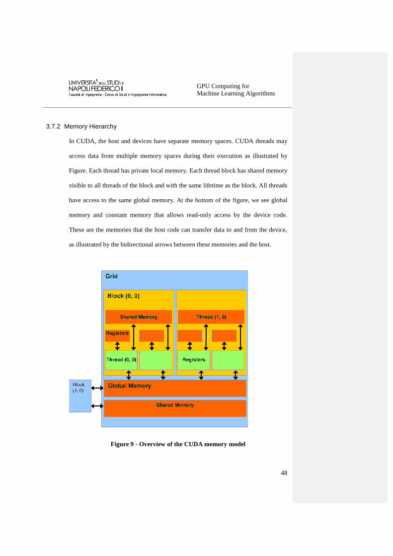
3.7.2 Memory Hierarchy
In CUDA, the host and devices have separate memory spaces. CUDA threads may
access data from multiple memory spaces during their execution as illustrated by
Figure. Each thread has private local memory. Each thread block has shared memory
visible to all threads of the block and with the same lifetime as the block. All threads
have access to the same global memory. At the bottom of the figure, we see global
memory and constant memory that allows read-only access by the device code.
These are the memories that the host code can transfer data to and from the device,
as illustrated by the bidirectional arrows between these memories and the host.
Figure 9 - Overview of the CUDA memory model

GPU Computing for Machine Learning Algorithms
49
3.7.3 Thread Hierarchy
Figure 10 - CUDA thread organization
When a kernel is invoked, it is executed as grid of parallel threads. Each CUDA
thread grid typically is comprised of thousands to millions of lightweight GPU
threads per kernel invocation. For simplicity, a small number of threads are shown
in Figure 10.
Threads in a grid are organized into a two-level hierarchy, where at the top level,
each grid consists of one or more thread blocks. All blocks in a grid have the same
number of threads. Each block has a unique two-dimensional coordinate given by

GPU Computing for Machine Learning Algorithms
50
the CUDA specific keywords blockIdx.x and blockIdx.y. All thread blocks must
have the same number of threads organized in the same manner. Blocks are
organized into a one-dimensional, two-dimensional, or three-dimensional array of
threads. On current GPUs a thread block may contain up to 1024 threads. Threads
with the same threadIdx values from different blocks would end up accessing the
same input and output data elements. When the host code invokes a kernel, it sets
the grid and thread block dimensions via execution configuration parameters.
3.7.4 CUDA C Parallel Programming Model
The introduction of multicore CPUs and manycore GPUs introduced the challenge is
to develop application software that transparently scales its parallelism to leverage
the increasing number of processor cores.
The CUDA parallel programming model is designed to overcome this challenge
while maintaining a low learning curve for programmers familiar with standard
programming languages such as C.
At its core are three key abstractions: a hierarchy of thread groups, shared memories,
and barrier synchronization.
These abstractions provide fine-grained data parallelism and thread parallelism,
nested within coarse-grained data parallelism and task parallelism. They guide the
programmer to partition the problem into coarse sub-problems that can be solved
independently in parallel by blocks of threads, and each sub-problem into finer
pieces that can be solved cooperatively in parallel by all threads within the block.

GPU Computing for Machine Learning Algorithms
51
This decomposition preserves language expressivity by allowing threads to
cooperate when solving each sub-problem, and at the same time enables automatic
scalability. Indeed, each block of threads can be scheduled on any of the available
processor cores, in any order, concurrently or sequentially, so that a compiled
CUDA program can execute on any number of processor cores as illustrated by
Figure 9, and only the runtime system needs to know the physical processor count.
Figure 11 – CUDA with different multi-core architectures
This scalable programming model is designed for transparent and portable
scalability. It allows the CUDA architecture to span a wide market range, from the
high-performance Tesla GPUs to the inexpensive mainstream GeForce GPUs, by

GPU Computing for Machine Learning Algorithms
52
scaling the number of processors and memory partitions. A CUDA program is
written once and runs on a GPU with any number of processor cores.
3.7.5 CUDA Program Structure
A CUDA program consists of one or more phases that are executed on either the
host (CPU) or a device such as a GPU. The phases that exhibit little or no data
parallelism are implemented in host code. The phases that exhibit rich amount of
data parallelism are implemented in the device code.
A CUDA program is a unified source code encompassing both host and device code.
While the host code is straight ANSI C code, the device code is written using ANSI
C extended with keywords for labeling data-parallel functions, called kernels, and
their associated data structures. The kernels typically generate a large number of
threads to exploit data parallelism. Due to efficient hardware support the CUDA
threads are of much fast and lighter weight than the CPU threads that typically
require thousands of clock cycles to generate and schedule.
The execution of a typical CUDA program starts with host (CPU) execution. When
a kernel function is invoked, the execution is moved to a device (GPU), where a
large number of threads are generated to take advantage of abundant data
parallelism. All the threads that are generated by a kernel during an invocation are
collectively called a grid. When all threads of a kernel complete their execution, the
corresponding grid terminates, and the execution continues on the host until another
kernel is invoked.

GPU Computing for Machine Learning Algorithms
53
Figure 12 - CUDA program structure
3.7.6 Other GPGPU environment: OpenCL
Recently, some collaboration between major industries, including Apple, Intel,
AMD (formerly ATI) and NVIDIA developed a programming model for
development on heterogeneous architectures across CPU, GPU and other types of
processors, called OpenCL (Open Computing Language). OpenCL will form the

GPU Computing for Machine Learning Algorithms
54
foundation layer of a parallel computing ecosystem of platform-independent tools,
middleware and applications.
OpenCL has been proposed as an open standard. Similar to CUDA, OpenCL
programming model defines a language, based on the C99 programming language
with extensions and restrictions, and runtime APIs to allow programmers the
management of data parallelism and massively parallel processors13.
OpenCL, being a standardized programming model, allows all applications,
requiring to be developed in this language, to be executed without any modification
to the code, on all devices that support language extensions and APIs.
OpenCL is a technology less known than CUDA. Its level of programming rules is
still less advanced than in CUDA and it is more complex to be used, due to the
absence of a unified SDK (Software Development Kit) to be shared among all
manufacturers.
Furthermore, on the platforms supporting both technologies, the speed reached by
OpenCL applications is still less than CUDA, an important factor influencing
developers, always demanding higher processing speed.
For completeness, we mention the development environments created by ATI: CTM
(Close To Metal) and Stream. These two programming models have been early
abandoned in favor of OpenCL, whose basic positive and negative features can be
summarized as follows:
13 http://www.khronos.org/registry/cl/sdk/1.0/docs/man/xhtml/

GPU Computing for Machine Learning Algorithms
55
Pros
• Acceleration in parallel processing;
• It allows to manage computational resources
o View multi-core CPUs, GPUs, etc. as computational units;
o Allocate different levels of memory;
• Cross-vendor software portability
o Separation of low-level and high-level software;
• Much wider range of hardware and platform support;
o Supports AMD, NVIDIA and Intel GPUs equally. It can also be used on
newer versions of Android phones, iPhones and other devices;
• It can fallback on CPU if the GPU support does not exist;
o In reality, to create thousands of threads on the CPU, it is generally not a good
idea;
• Supports synchronization over multiple devices;
• Easy to get started with integrating OpenCL kernels in to the code.
• An open standard and not vendor locked and a kernel language based on C99
specification.
Con
• public drivers to support OpenCL 1.1. Currently only developer ones exist;
• Lacks mature libraries;
• Debugging and profiling tools are not as advanced as CUDAs.
Moreover, the following table reports a direct comparison between OpenCL and CUDA
(Rosendahl 2010).
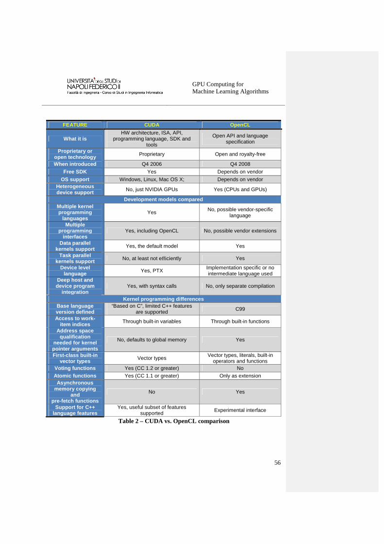
GPU Computing for Machine Learning Algorithms
56
FEATURE CUDA OpenCL
What it is HW architecture, ISA, API,
programming language, SDK and tools
Open API and language specification
Proprietary or open technology Proprietary Open and royalty‐free
When introduced Q4 2006 Q4 2008
Free SDK Yes Depends on vendor
OS support Windows, Linux, Mac OS X; Depends on vendor Heterogeneous device support No, just NVIDIA GPUs Yes (CPUs and GPUs)
Development models compared Multiple kernel programming
languages Yes No, possible vendor‐specific
language
Multiple programming
interfaces Yes, including OpenCL No, possible vendor extensions
Data parallel kernels support Yes, the default model Yes
Task parallel kernels support No, at least not efficiently Yes
Device level language Yes, PTX
Implementation specific or no intermediate language used
Deep host and device program
integration Yes, with syntax calls No, only separate compilation
Kernel programming differences Base language version defined
“Based on C”, limited C++ features are supported C99
Access to work ‐‐‐‐item indices Through built‐in variables Through built‐in functions
Address space qualification
needed for kernel pointer arguments
No, defaults to global memory Yes
First ‐‐‐‐class built ‐‐‐‐in vector types Vector types Vector types, literals, built-in
operators and functions Voting functions Yes (CC 1.2 or greater) No
Atomic functions Yes (CC 1.1 or greater) Only as extension Asynchronous
memory copying and
pre-fetch functions
No Yes
Support for C++ language features
Yes, useful subset of features supported
Experimental interface
Table 2 – CUDA vs. OpenCL comparison

GPU Computing for Machine Learning Algorithms
57
4 Technology in machine learning
The sheer size of the foreseen data streams renders impossible to discriminate
objects using traditional software tools, and requires the development of specific
computing infrastructures as well as the implementation of specific and robust
(largely based on the ML paradigm) methods for data analysis and understanding.
ML methods, in order to provide efficient and reliable answers, need also to exploit
all the meta-information made available to any scientific/social community through
the data repositories federated under specific data centers or virtual organizations
(Genova et al. 2002).
The problem of inventing and deploying these new tools under powerful
computational infrastructure has therefore become a worldwide challenge. On the
algorithmic side, we wish to emphasize that commonly used decision algorithms
depend on a fixed number of predefined input features for decision making. This is
not the best option in Time Domain Analysis where some of the inputs may not be
present within the time slot available to make the decision.
There is therefore a demand for a completely new class of tools that can dynamically
select the input features and can consistently give reliable predictions. Most decision
algorithms compute the inverse Bayesian probability to deal with missing attributes
(mostly called features) in the input data.

GPU Computing for Machine Learning Algorithms
58
Although such algorithms can handle missing features to some extent, there is
always a possibility for asymptotic decline in accuracy. It may be argued that the
possible state of the missing feature can be adequately constrained and compensated
for by the available remaining inputs.
However this is not true, because a feature that can be well constrained by the
remaining inputs is usually redundant and it is not required as an input at the first
place. If this is not the case, its absence can't be appropriately compensated and that
will result in a loss of information.
The idea therefore is to facilitate dynamic learning in which, for instance, the system
learns from all available information (and not on a fixed set of samples) and identify
strategies that can optimally handle situations in which most of the inputs are
missing.
As already underlined, one of next main breakthroughs in many human fields is that
we have reached the physical limit of observations. So far, like all scientific
disciplines focusing their discoveries on collected data exploration, there is a strong
need to employ e-science methodology and tools in order to gain new insights on the
knowledge. But this mainly depend on the capability to recognize patterns or trends
in the parameter space (i.e. physical laws), possibly by overcoming the human limit
of 3D brain vision, and to use known patterns as Base of Knowledge (BoK) to infer
knowledge on self-adaptive models in order to make them able to generalize feature
correlations and to gain new discoveries (for example outliers identification) through
the unbiased exploration of new collected data. These requirements are perfectly
matching the paradigm of ML techniques based on the Artificial Intelligence

GPU Computing for Machine Learning Algorithms
59
postulate (Bishop 2006). Hence, in principle at all steps of an exploration workflow
ML rules can be applied. Let us better know this methodology.
There is a basic dichotomy in ML, by distinguish between supervised and
unsupervised methodology, as described in the following.
The Greek philosopher Aristotle was one of the first to attempt to codify "right
thinking," that syllogism is, irrefutable reasoning processes. His syllogisms provided
patterns for argument structures that always yielded correct conclusions when given
correct premises. For example, "Socrates is a man; all men are mortal; therefore,
Socrates is mortal." These laws of thought were logic supposed to govern the
operation of the mind; their study initiated the field called logic. Logicians in the
19th century developed a precise notation for statements about all kinds of things in
the world and about the relations among them. Contrast this with ordinary arithmetic
notation, which provides mainly for equality and inequality statements about
numbers.
By 1965, programs existed that could, in principle, process any solvable problem
described in logical notation (Moore 1965). The so-called logicist tradition within
artificial intelligence hopes to build on such programs to create intelligent systems
and the ML theory represents their demonstration discipline. Reinforcement in this
direction came out by integrating ML paradigm with statistical principles following
the Darwin’s Nature evolution laws, (Duda et al. 2001).

GPU Computing for Machine Learning Algorithms
60
4.1 The learning paradigms
In supervised ML we have a set of data points or observations for which we know
the desired output, expressed in terms of categorical classes, numerical or logical
variables or as generic observed description of any real problem. The desired
output is in fact providing some level of supervision in that it is used by the learning
model to adjust parameters or make decisions allowing it to predict correct output
for new data. Finally, when the algorithm is able to correctly predict observations
we define it a classifier. Some classifiers are also capable of providing results in a
more probabilistic sense, i.e. a probability of a data point belonging to class. We
usually refer to such model behavior as regression.
A typical workflow for supervised learning is shown in the diagram below (Figure
13).
Figure 13 – A workflow based on supervised learning paradigm
The process is:

GPU Computing for Machine Learning Algorithms
61
• Pre-processing of data. First we need to build input patterns that are appropriate
for feeding into our supervised learning algorithm. This includes scaling and
preparation of data;
• Create data sets for training and evaluation. This is done by randomly splitting
the universe of data patterns. The training set is made of the data used by the
classifier to learn their internal feature correlations, whereas the evaluation set is
used to validate the already trained model in order to get an error rate (or other
validation measures) that can help to identify the performance and accuracy of the
classifier. Typically you will use more training data than validation data;
• Training of the model. We execute the model on the training data set. The output
result consists of a model that (in the successful case) has learned how to predict
the outcome when new unknown data are submitted;
• Validation. After we have created the model, it is of course required a test of its
performance accuracy, completeness and contamination (or its dual, the purity). It
is particularly crucial to do this on data that the model has not seen yet. This is
main reason why on previous steps we separated the data set into training patterns
and a subset of the data not used for training. We intend to verify and measure the
generalization capabilities of the model. It is very easy to learn every single
combination of input vectors and their mappings to the output as observed on the
training data, and we can achieve a very low error in doing that, but how does the
very same rules or mappings perform on new data that may have different input to
output mappings? If the classification error of the validation set is higher than the
training error, then we have to go back and adjust model parameters. The reason
could be that the model has essentially memorized the answers seen in the training
data, failing its generalization capabilities. This is a typical behavior in case of
overfitting, and there are various techniques for overcoming it;

GPU Computing for Machine Learning Algorithms
62
• Use. If validation was successful the model has correctly learned the underlying
real problem. So far we can proceed to use the model to classify/predict new data.
The kinds of problems that are suited for unsupervised algorithms may seem similar,
but are very different to supervised learners. Instead of trying to predict a set of
known classes, we are trying to identify the patterns inherent in the data that
separate like observations in one way or another. In other words, the main difference
is that we are not providing a target variable like we did in supervised learning.
This marks a fundamental difference in how both types of algorithms operate. On
one hand, we have supervised algorithms which try to minimize the error in
classifying observations, while unsupervised learning algorithms don't have such
gain, because there are no outcomes or target labels. Unsupervised algorithms try to
create clusters of data that are inherently similar. In some cases we don't necessarily
know what makes them similar, but the algorithms are capable of finding
relationships between data points and group them in possible significant ways.
Differently from supervised algorithms, which aim at minimizing the classification
error, unsupervised algorithms try to create groups or subsets of the data, in which
points belonging to a cluster are as similar to each other as possible, by making the
difference between the clusters as high as possible (Haykin 1998).
Another main difference is that in an unsupervised problem, the concept of training set does not apply in the same way as with supervised learners. Typically we have a data set that is used to find the relationships in the data that buckets them in different clusters. A common workflow approach for unsupervised learning analysis is shown in the diagram below (Figure 14).

GPU Computing for Machine Learning Algorithms
63
Figure 14 – A workflow based on unsupervised learning paradigm
For unsupervised learning, the process is:
1) Pre-processing of data. As with supervised learners, this step includes selection of
features to feed into the algorithm, by also scaling them to build a suitable training
data set;
2) Execution of model training. We run the unsupervised algorithm on the scaled
data set to get groups of like observations;
3) Validation. After clustering the data, we need to verify whether it cleanly
separated the data in significant ways. This includes calculating a set of statistics
on the resulting outcomes, as well as analysis based on domain knowledge, where
you may measure how certain features behave when aggregated by the clusters.
Once we are satisfied of the resulting creation of clusters (or in general over-
densities), there is no need to run the model with new data (although you can).

GPU Computing for Machine Learning Algorithms
64
4.2 What we are looking for in the data
In the DM scenario, the ML model choice should always be accompanied by the
functionality domain. To be more precise, some ML models can be used in a same
functionality domain, because it represents the functional context in which it is
performed the exploration of data.
Traditional statistical methods break down partly because of the increase in the
number of observations, but mostly because of the increase in the number of
variables associated with each observation. The dimension of the data is the number
of variables that are measured on each observation.
High-dimensional data sets present many mathematical challenges as well as some
opportunities, and are bound to give rise to new theoretical developments. One of
the problems with high-dimensional data sets is that, in many cases, not all the
measured variables are “important” for understanding the underlying phenomena of
interest. While certain computationally expensive novel methods can construct
predictive models with high accuracy from high-dimensional data, it is still of
interest in many applications to reduce the dimension of the original data prior to
any data modeling (Samet 2006).
In mathematical terms, the problem we investigate can be stated as follows: given
the p-dimensional random variable � = ���,⋯ , ��, and a lower dimensional
representation of it, � = ���,⋯ , � � with k ≤ p, that captures the content in the
original data, according to some criterion. The components of s are sometimes called
the hidden components. Different fields use different names for the p multivariate

GPU Computing for Machine Learning Algorithms
65
vectors: the term “variable” is mostly used in statistics, while “feature” and
“attribute” are alternatives commonly used in the DM and ML literature.
Generally speaking, dimensional reduction is the process of reducing the number of
random variables under consideration, and can be divided into feature
selection and feature extraction.
Feature selection approaches try to find a subset of the original variables (also called
features or attributes) (Guyon et al. 2003). Two strategies are filter (e.g. information
gain) and wrapper (e.g. search guided by the accuracy) approaches.
Feature extraction transforms the data in the high-dimensional space to a space of
fewer dimensions. The data transformation may be linear, as in Principal
Component Analysis (PCA), but many non-linear techniques also exist (Guyon et al.
2006).
Being based on the covariance matrix of the variables, PCA is a second-order
method. In various fields, it is also known as the Singular Value Decomposition
(SVD), the Karhunen-Loève transform, the Hotelling transform, and the Empirical
Orthogonal Function (EOF) method. In essence, PCA seeks to reduce the dimension
of the data by finding a few orthogonal linear combinations (Principal Components)
of the original variables with the largest variance. In other words, PCA performs a
linear mapping of the data to a lower dimensional space in such a way that the
variance of the data in the low-dimensional representation is maximized.
Another technique belonging, like PCA, to the latent variable methods family, is the
model known as Principal Probabilistic Surfaces (PPS), in which first principal
component accounts for as much of the variability in the data as possible, and each
GPU Computing for Machine Learning Algorithms
66
succeeding component accounts for as much of the remaining variability as possible
(Chang et al. 2001).
The PPS are able to find a better data aggregation than the PCA method. A PPS is
trained to recognize the best projection functions from the N-dimensional parameter
space to a spherical surface in a 3D space.
This surface is covered by a grid of latent variables (points), representing the
Gaussian peak in the N-parameter space. It permits to visualize all data with a
human compliant 3D diagram, independently from the number of initial parameters.
It is hence possible to individuate the presence of sub-structures in the data. An
interesting aspect is the estimation of each input data parameter incidence on the
latent variables that can help to understand the relationship between the parameter
and the found clusters. The incidence of parameters is calculated by evaluating the
probability density of input vector components in respect of each latent variable.
During the training phase a reference variety is created.
In the test phase, a datum, never seen by the network, is attributed to the closest
spherical variety. Obviously the concept of closest implies a calculation of a
distance between a point and a node in the space. Before that the data must be
projected on the space. This basically because a spherical variety consists of squared
or triangular areas, each of them defined by 3 or 4 variety nodes. After this
projection of the datum the approximated distance is calculated.
In the PPS system three main approximation criteria exist:
• Nearest Neighbor: it founds the minimum square distance from all variety nodes;
• Grid projections: it founds the shortest projection distance on the variety grid;

GPU Computing for Machine Learning Algorithms
67
• Nearest Triangulation: it founds the projection closest to the possible
triangulations.
The most frequently used is the first one, because it permits to evaluate the distances
between data and all nodes on the spherical variety. The downside is that it is
generally more time-consuming, but more precise than others (LeBlanc et al. 1994).
The technique described above makes clear the role of PPS as an efficient method
for MDS pre-clustering or dimensional reduction.
More generally, the advantage to preliminarily apply a dimensional reduction model
to data is that, in some cases, data analysis such as regression or classification can be
done in the reduced space more accurately than in the original one.
Classification is a procedure in which individual items are placed into groups based
on quantitative information on one or more features inherent to the items (referred to
as features) and based on a training set of previously labeled items (Kotsiantis
2007).
A classifier is a system that performs a mapping from a feature space X to a set of
labels Y. Basically a classifier assigns a pre-defined class label to a sample.
Formally, the problem can be stated as follows: given training data
����, ��,⋯ , ���, ��� (where �� are vectors) a classifier h:X → Y maps an object
xϵX to its classification label yϵY.
Different classification problems could arise:
a) crispy classification: given an input pattern x (vector) the classifier returns its
computed label y (scalar).

GPU Computing for Machine Learning Algorithms
68
b) probabilistic classification: given an input pattern x (vector) the classifier returns a
vector y which contains the probability of �� to be the "right" label for x. In other
words in this case we seek, for each input vector, the probability of its
membership to the class �� (for each��).
Both cases may be applied to both "two-class" and "multi-class" classification. So
the classification task involves, at least, three steps:
• training, by means of a training set (input: patterns and target vectors, or labels;
output: an evaluation system of some sort);
• testing, by means of a test set (input: patterns and target vectors, requiring a valid
evaluation system from point 1; output: some statistics about the test, confusion
matrix, overall error, bit fail error, as well as the evaluated labels);
• evaluation, by means of an unlabeled data set (input: patterns, requiring a valid
evaluation systems; output: the labels evaluated for each input pattern);
Because of the supervised nature of the classification task, the system performance
can be measured by means of a test set during the testing procedure, in which unseen
data are given to the system to be labeled.
The overall error somehow integrates information about the classification goodness.
However, when a data set is unbalanced (when the number of samples in different
classes varies greatly) the error rate of a classifier is not representative of the true
performance of the classifier. A confusion matrix can be calculated to easily
visualize the classification performance (Provost et al. 1998): each column of the
matrix represents the instances in a predicted class, while each row represents the

GPU Computing for Machine Learning Algorithms
69
instances in an actual class. One benefit of a confusion matrix is the simple way to
see if the system is mixing two classes.
Optionally (some classification methods does not require it by its nature or simply as
a user choice), one could need a validation procedure.
Validation is the process of checking if the classifier meets some criterion of
generality when dealing with unseen data. It can be used to avoid over-fitting or to
stop the training on the base of an "objective" criterion.
With “objective” we intend a criterion which is not based on the same data we have
used for the training procedure. If the system does not meet this criterion it can be
changed and then validated again, until the criterion is matched or a certain
condition is reached (for example, the maximum number of epochs). There are
different validation procedures. One can use an entire data set for validation
purposes (thus called validation set); this data set can be prepared by the user
directly or in an automatic fashion.
In some cases (e.g. when the training set is limited) one could want to apply a “cross
validation” procedure, which means partitioning a sample of data into subsets such
that the analysis is initially performed on a single subset, while the other subset(s)
are retained for subsequent use in confirming and validating the initial analysis
(Mosteller et al. 1968). Different types of cross validation may be implemented, e.g.
k-fold, leave-one-out, etc.
Summarizing we can safely state that a common classification training task
involves:
• the training set to compute the model;

GPU Computing for Machine Learning Algorithms
70
• the validation set to choose the best parameters of this model (in case there are
"additional" parameters that cannot be computed based on training);
• the test data as the final “judge”, to get an estimate of the quality on new data that
are used neither to train the model, nor to determine its underlying parameters or
structure or complexity of this model;
The validation set may be provided by the user, extracted from the software or
generated dynamically in a cross validation procedure. In the next paragraphs we
underline some practical aspects connected with the validation techniques for
classification models.
Regression methods bring out relations between variables, especially whose relation
is imperfect (i.e. it has not one y for each given x). The term regression is
historically coming from biology in genetic transmission through generations, where
for example it is known that tall fathers have tall sons, but not as tall on the average
as the fathers. The trend to transmit on average genetic features, but not exactly in
the same quantity, was what the scientist Galton defined as regression, more exactly
regression toward the mean (Galton 1877).
But what is regression? Strictly speaking it is very difficult to find a precise
definition. It seems the existence of two meanings for regression (Hastie et al. 2005),
that can be addressed as data table statistical correlation (usually column averages)
and as fitting of a function.
About the first meaning, let start with a very generic example: let’s suppose to have
two variables x and y, where for each small interval of x there is a distribution of
corresponding y. We can always compute a summary of the y values for that

GPU Computing for Machine Learning Algorithms
71
interval. The summary might be for example the mean, median or even the
geometric mean. Let fix the points ���, ��� ), where �� is the center of the ith interval
and ��� the average y for that interval. Then the fixed points will fall close to a curve
that could summarize them, possibly close to a straight line. Such a smooth curve
approximates the regression curve called the regression of y on x. By generalizing
the example, the typical application is when the user has a table (let say a series of
input patterns coming from any experience or observation) with some
correspondences between intervals of x (table rows) and some distributions of y
(table columns), representing a generic correlation not well known (i.e. imperfect as
introduced above) between them. Once we have such a table, we want for example
to clarify or accent the relation between the specific values of one variable and the
corresponding values of the other. If we want an average, we might compute the
mean or median for each column. Then to get a regression, we might plot these
averages against the midpoints of the class intervals.
Given the example in mind let’s try to extrapolate the formal definition of regression
(in its first meaning).
In a mathematical sense, when for each value of x there is a distribution of y, with
density f(y|x) and the mean (or median) value of y for that x given by:
���� = � � ��|�"�#$%$ (1)
then the function defined by the set of ordered pairs ��, ���� is called the
regression of y on x. Depending on the statistical operator used, the resulting
regression line or curve on the same data can present a slightly different slope.

GPU Computing for Machine Learning Algorithms
72
Sometimes we do not have continuous populations with known functional forms.
But the data may be very extensive (such as in the astrophysical case). In these cases
it is possible to break one of the variables into small intervals and compute averages
for each of them. Then, without severe assumptions about the shape of the curve,
essentially get a regression curve. What the regression curve does is essentially to
give a, let say, “big summary” for the averages for the distributions corresponding to
the set of x’s. One can go further and compute several different regression curves
corresponding to the various percentage points of the distributions and thus get a
more complete picture of the input data set. Of course often it is an incomplete
picture for a set of distributions! But in this first meaning of regression, when the
data are more sparse, we may find that sampling variation makes impractical to get a
reliable regression curve in the simple averaging way described (Menard 2001).
From this assumption, it descends the second meaning of regression.
Usually it is possible to introduce a smoothing procedure, applying it either to the
column summaries or to the original values of y’s (of course after an ordering of y
values in terms of increasing x). In other words we assume a shape for the curve
describing the data, for example linear, quadratic, logarithmic or whatever. Then we
fit the curve by some statistical method, often least-squares. In practice, we do not
pretend that the resulting curve has the perfect shape of the regression curve that
would arise if we had unlimited data, but simply we obtain an approximation. In
other words we intend the regression of data in terms of forced fitting of a functional
form. The real data present intrinsic conditions that make this second meaning as the
official regression use case, instead of the first, i.e. curve connecting averages of

GPU Computing for Machine Learning Algorithms
73
column distributions. We ordinarily choose for the curve a form with relatively few
parameters and then we have to choose the method to fit it. In many manuals
sometimes it might be founded a definition probably not formally perfect, but very
clear: by regressing one y variable against one x variable means to find a carrier for
x. This introduces possible more complicated scenarios in which more than one
carrier of data can be founded. In these cases it has the advantage that the geometry
can be kept to three dimensions (with two carriers) up to n-dimensional spaces (n >
3, with more than two carriers regressing input data). Clearly, both choosing the set
of carriers from which a final subset is to be drawn and choosing that subset can be
most disconcerting processes.
In substance we can declare a simple, important use of regression, consisting in:
To get a summary of data, i.e. to locate a representative functional operator of the
data set, in a statistical sense (first meaning) or via an approximated trend curve
estimation (second meaning).
And a more common use of regression:
• For evaluation of unknown features hidden into the data set;
• For prediction, as when we use information from several weather or astronomical
seeing stations to predict the probability of rain or the turbulence growing in the
atmosphere;
• For exclusion. Usually we may know that x affects y, and one could be curious to
know whether z is associated with y too, through a possible casual mechanism. In
this case one approach would take the effects of x out of y and see if what remains
is associated with z. In practice this can be done by an iterative fitting procedure
by evaluating at each step the residual of previous fitting.

GPU Computing for Machine Learning Algorithms
74
This is not exhaustive of the regression argument, but simple considerations to help
the understanding of the regression term and the possibility to extract basic
specifications for the use case characterization in the design phase.
Clustering is a division of data into groups of similar objects. Representing the data
by fewer clusters necessarily loses certain fine details (data compression), but
achieves simplification (Jain et al. 1999).
From a ML perspective clusters correspond to hidden patterns, the search for
clusters is unsupervised learning, and the resulting system could represent a data
concept in the KDD (Knowledge Discovery in Databases).
From a practical perspective clustering plays an outstanding role in DM applications
such as scientific data exploration, information retrieval and text mining, spatial
database applications, Web analysis, Customer Relationships Management (CRM),
marketing, medical diagnostics, computational biology, and many others.
For example, in CRM, marketing applications generally come with predictive
clustering analytics to improve segmentation and targeting, and features for
measuring the effectiveness of online, offline, and search marketing campaigns
(Collica 2007). By evaluating “buy signals,” marketers can see which prospects are
most likely to transact and also identify those who are bogged down in a sales
process and need assistance.
Data mining on MDS adds to clustering the complications of very large data sets
with very many attributes of different types (high dimensionality). This imposes
unique computational requirements on relevant clustering algorithms.

GPU Computing for Machine Learning Algorithms
75
What are the properties of clustering algorithms we are concerned with in DM?
These properties include:
• Type of attributes that the algorithm can handle;
• Scalability to large data sets;
• Ability to work with high dimensional data (multi-D parameter space, multi-
wavelength, multi-epoch etc…);
• Ability to find clusters of irregular shape;
• Handling outliers;
• Time complexity (when there is no confusion, we use the term complexity);
• Data order dependency;
• Labeling or assignment (hard or strict vs. soft of fuzzy);
• Reliance on a priori knowledge and user defined parameters;
• Interpretability of results;
We have to try to keep these issues in mind, realistically. The above list is in no way
exhaustive. For example, we must deal also with implementation properties, such as
ability to work in pre-defined memory buffer, ability to restart and to provide an
intermediate solution and so on.
4.3 Learning Strategies
Before going into the working mechanisms of ML systems, it is interesting and
useful to focus the attention on the shape and expressions of data to be given as
input to ML information processing models.

GPU Computing for Machine Learning Algorithms
76
In ML experiments the performance strongly depends from data used for training.
Hence it is crucial the choice of data selection and their representation mode.
Generally, except for some particular cases, the set of input data is provided under
the form of tables or matrices; in which any row identify an example (a complete
pattern in the data parameter space), whose columns are all parameters (features)
and their values the parameter attributes.
It may be frequent that the table can have empty entries (sparse matrix) or missing
(lack of observed values for some features in some patterns). It may also happen that
information of a single table is not homogeneous, i. e. attributes may be of different
types, such as numerical mixed with categorical entries.
This level of diversity in the internal information could be also related with different
format type of data sets, such as tables registered in ASCII code (ANSI et al. 1977),
CSV (Comma Separated Values) (Repici 2002) or FITS (text header followed by
binary code of an image) (Wells et al. 1981).
In order to reach an efficient and homogeneous representation of data sets, to be
submitted to ML systems, it is mandatory to preliminarily take care of the data
format, in order to make them intelligible by the processing framework. In other
words to transform pattern features to assume a uniform representation before to
submit them to the training process.
In this mechanism the real situations could be very different. Let think to time
sequences (coming from any sensor monitoring acquisition), where data are
collected in a single long sequence, not simply divisible, or to raw data (such as

GPU Computing for Machine Learning Algorithms
77
original images taken by astronomical observations), that could be affected by noise
or aberration factors.
These events always require a pre-processing phase, to clean and opportunely
prepare the data sets to be used for any ML and DM experiment. Of course such
preliminary step must take into account also the functional scope of the experiment
itself.
More in practice, having in mind the functional taxonomy described in the previous
section, there are essentially four kinds of learning related with ML for DM:
1) Learning by association;
2) Learning by classification;
3) Learning by prediction;
4) Learning by grouping (clustering);
The primer, learning by association consists of the identification of any structure
hidden between data. It does not mean to identify the belonging of patterns to
specific classes, but to predict values of any feature attribute, by simply recalling it,
i.e. by associating it to a particular state or sample of the real problem.
It is evident that in the case of association we are dealing with very generic
problems, i.e. those requiring a precision less than in the classification case. In fact,
the complexity grows with the range of possible multiple values for feature
attributes, potentially causing a mismatch in the association results.
In practical terms, fixed percentage thresholds are given in order to reduce the
mismatch occurrence for different association rules, based on the experience on that

GPU Computing for Machine Learning Algorithms
78
problem and related data. The representation of data for associative learning is thus
based on the labeling of features with non-numerical values or by alpha-numeric
coding.
Classification learning is often named simply “supervised” learning, because the
process to learn the right assignment of a label to a datum, representing its category
or “class”, is usually done by examples. Learning by examples stands for a training
scheme operating under supervision of any oracle, able to provide the correct,
already known, outcome for each of the training sample. And this outcome is
properly a class or category of the examples. Its representation depends on the
available Base of Knowledge (BoK) and on its intrinsic nature, but in most cases is
based on a series of numerical attributes, related to the extracted BoK, organized and
submitted in a homogeneous way.
The success of classification learning is usually evaluated by trying out the acquired
feature description on an independent set of data, having known output but never
submitted to the model before.
Slightly different from classification scheme is the prediction learning. In this case
the outcome consists of a numerical value instead of a class.
The numeric prediction is obviously related to a quantitative result, because is the
predicted value much more interesting than the structure of the concept behind the
numerical outcome.
Whenever there is no any class attribution, clustering learning is used to group data
that show natural similar features. Of course the challenge of a clustering
experiment is to find these clusters and assign input data to them. The data could be

GPU Computing for Machine Learning Algorithms
79
given under the form of categorical/numerical tables and the success of a clustering
process could be evaluated in terms of human experience on the problem or a
posteriori by means of a second step of the experiment, in which a classification
learning process is applied in order to learn an intelligent mechanism on how new
data samples should be clustered.
In the wide variety of possible applications for ML, DM is of course one of the most
important, but also the most challenging. Users encounter as much problems as
massive is the data set to be investigated. To find hidden relationships between
multiple features in thousands of patterns is hard, especially by considering the
limited capacity of human brain to have a clear vision in a multiple than 3D
parameter space.
Artificial neural networks are one of the best examples of ML methods, inspired by
the human brain architecture and learning rules. Dealing with supervised learning,
these models need training patterns formed by feature-target couples. Indeed for
each given input pattern (list of features), there should be also given the
corresponding list of targets (one or more). We already called such a complete data
set as Base of Knowledge (BoK). With this data set, the network could be able to
learn the right association between input features and location of its output in the
parameter space. The network will be able, after this training process, to correctly
classify any pattern, even if not presented to the network in the training phase
(generalization).
One of the simplest models of supervised neural networks is the Perceptron
(Rosenblatt 1957), composed by a single output neuron and N input neurons. The

GPU Computing for Machine Learning Algorithms
80
capabilities of this model are very limited, but it is a good starting point for more
advanced and complex variants of such network. The network learns by modifying
the weights to enforce right decisions and discourage those wrong. At each iteration
a new pattern of the training set is presented and the network calculates its output.
Main limit of such model is that it is able to correctly classify the input only if
classes are linearly separable (see Figure 15a). However the division between
classes is much more complex. A typical example is a problem (see Figure 15b),
where it is not possible to find a single split line for the two classes and the
Perceptron fails.
Figure 15 – correct (a) and wrong (b) separation of classes made by a
Perceptron
To overcome this problem it is needed to employ more complex classification
structures, organized on more than one computational layer (Cybenko 1989).
In order to be able to operate non-linear classification, i.e. to separate complex
regions, the solution is to extend the perceptron to the so-called Multi-Layer
Perceptron (MLP), a network composed by one or more hidden layers of neuron,
fully connected, between input and output layers (Figure 16).

GPU Computing for Machine Learning Algorithms
81
Figure 16 – Regions recognized by a MLP with 0, 1, 2 hidden layers
The classical topology of MLP is shown in Figure. This kind of networks is able to
recognize and classify any type of topological region, having as downside a more
complex learning process. Moreover, the Heaviside function cannot be applied as
activation function, because it is not differentiable. An alternative is to use the
sigmoid function. In this case the activation values of output neurons become
differentiable functions of input values and hidden neuron weights.
The practice and expertise in the ML methods, such as MLP, are important factors,
formed through a long exercise within scientific experiments. In particular the speed
and effectiveness of the results strongly depend on these factors. Unfortunately there
are no magic ways to a priori indicate the best configuration of internal parameters,
involving network topology and learning algorithm, but a series of heuristics.
Figure 17 – Classical topology of a MLP with hidden neurons in white circles
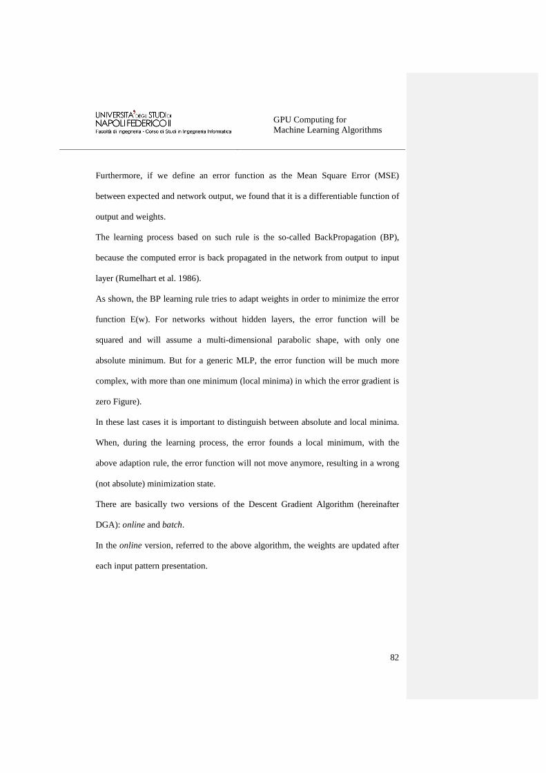
GPU Computing for Machine Learning Algorithms
82
Furthermore, if we define an error function as the Mean Square Error (MSE)
between expected and network output, we found that it is a differentiable function of
output and weights.
The learning process based on such rule is the so-called BackPropagation (BP),
because the computed error is back propagated in the network from output to input
layer (Rumelhart et al. 1986).
As shown, the BP learning rule tries to adapt weights in order to minimize the error
function E(w). For networks without hidden layers, the error function will be
squared and will assume a multi-dimensional parabolic shape, with only one
absolute minimum. But for a generic MLP, the error function will be much more
complex, with more than one minimum (local minima) in which the error gradient is
zero Figure).
In these last cases it is important to distinguish between absolute and local minima.
When, during the learning process, the error founds a local minimum, with the
above adaption rule, the error function will not move anymore, resulting in a wrong
(not absolute) minimization state.
There are basically two versions of the Descent Gradient Algorithm (hereinafter
DGA): online and batch.
In the online version, referred to the above algorithm, the weights are updated after
each input pattern presentation.
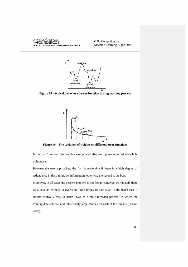
GPU Computing for Machine Learning Algorithms
83
Figure 18 – typical behavior of error function during learning process
Figure 19 – The variation of weights on different error functions
In the batch version, the weights are updated after each presentation of the whole
training set.
Between the two approaches, the first is preferable if there is a high degree of
redundancy in the training set information, otherwise the second is the best.
Moreover, in all cases the descent gradient is not fast to converge. Fortunately there
exist several methods to overcome these limits. In particular, in the batch case it
results relatively easy to make DGA as a multi-threaded process, in which the
training data sets are split into equally large batches for each of the threads (Heaton
2009).

GPU Computing for Machine Learning Algorithms
84
Both versions require that the learning rate is a priori defined in a static way. This is
another important point, because a high value of learning rate causes a more instable
convergence of the learning process (the error function jumps along the error surface
without convergence assurance). For a learning rate too small, the convergence will
result extremely slowly.
The good compromise is to gradually reduce, at each learning step, the value of the
learning rate (for example by simply following the law & = 1 (⁄ or by applying more
complex rules), obtaining a faster convergence of the algorithm (Jacobs 1988).
By using the standard DGA, the direction of each updating step is calculated through
the error descent gradient, while the length is determined by the learning rate. A
more sophisticated approach could be to move towards the negative direction of the
gradient (line search direction) not by a fixed length, but up to reach the minimum
of the function along that direction. This is possible by calculating the descent
gradient and analyzing it with the variation of the learning rate.
The problem of line search is in practice a single dimension minimization problem.
There exist many other methods to solve this problem. For example the parabolic
search of a minimum calculates the parabolic curve crossing pre-defined learning
rate points. The minimum d of the parabolic curve is a good approximation of the
minimum of E(λ) and it can be reached by considering the parabolic curve crossing
the fixed points with the lowest error values.
There are also the trust region based strategies to find a minimum of an error
function, which main concept is to iteratively growing or contracting the region of
the function by adjusting a quadratic model function which better approximates the

GPU Computing for Machine Learning Algorithms
85
error function. In this sense this technique is considered dual to line search, because
it tries to find the best size of the region by preliminarily fixing the moving step (the
opposite of the line search strategy that always chooses the step direction before to
select the step size), (Celis et al. 1985).
Up to now we have supposed that the optimal search direction for the method based
on the line search is given at each step by the negative gradient. That’s not always
true!
If the minimization is done along the negative gradient, next search direction (the
new gradient) will be orthogonal to the previous one. By selecting further directions
equal to the negative gradient, there should be obtained some oscillations on the
error function that slow down the convergence process. The solution could be to
select further more directions such that the gradient component, parallel to the
previous search direction (that is zero), remains unchanged at each step.
In the ML based on supervised paradigm, there is nowadays a considerable interest
in techniques based on margin regularization (Baxter 2000). The concept derives
from the assumption that the distance (typically Euclidean distance) of an example
from the separating hyperplane is the margin of that example and the final goal is to
find the best margin of separation (classification) for the submitted data. Significant
examples include the Support Vector Machine (SVM), (Cortes et al. 1995), a
powerful classification tool that has gained its popularity and interest due to its
theoretical merits and successes in real applications (Burges 1998).

GPU Computing for Machine Learning Algorithms
86
SVM were originally defined in order to classify two classes of objects linearly
separable. For each class SVM identify the hyperplane that maximize the margin of
separation (Figure 20).
In Figure 20 black dots are the first class, white dots the second class, the three lines
are three possible margins, it is obvious that H3 is not suitable for this problem, H1
separates the two class but it’s very near to some dots of the two class, H2 maximize
the distance from the dots and is the best separator.
Figure 20 – Parameter space separated by hyperplanes through SVM model
Another technique related with the supervised ML is the one including methods
called logic based algorithms. Main examples are decision trees or its derivation,
rule-based estimators.
We have already introduced decision trees in the previous sections. By dealing with
supervised learning, they try to classify patterns by sorting them on the base of their
feature values.
However they have some defects. First, the construction of optimal binary decision
trees is a well-known NP-complete problem (Hyafil et al. 1976), hence it requires
complex heuristics to overcome this limit. Second, for their nature decision trees are

GPU Computing for Machine Learning Algorithms
87
univariate, i.e. they split the parameter space on a single feature at each node,
revealing inefficient in case of diagonal partitioning requirements. The solution is
hence to use alternative multivariate trees, usually obtained by the combination
between linear discriminant method and decision trees (Brodley et al. 1995).
As known, it is always possible to derive a rule-based estimator by a decision tree,
simply associating one tree path to a separated rule.
One positive aspect of a decision tree is of course its comprehensibility and ease of
use. It is intuitive enough to understand that a decision tree corresponds to a
hierarchy of tests done by simply making the data flowing through the tree branches
and taking output at its leaves (Kotsiantis 2007).
In the unsupervised case, the learning mechanism has something apparently magic.
The data analysis model appears a closed system, except for the input data. It never
interacts with external environment neither receives any kind of target outputs, but it
learns!
Behind this apparently mysterious behavior, we can observe that the unsupervised
learning consists in the internal re-organization of the input, based on the retrieved
correlations hidden into the data by some quantities of unknown noise contributions.
In a certain way, unsupervised learning can be interpreted as a self-adaptive
mechanism to find patterns in the data beyond what can be considered pure
unstructured noise (Gharamani 2004). Two important classic functional examples of
such learning type are clustering and dimensional reduction.
Almost all unsupervised methods may be considered strictly connected with
statistical and probabilistic issues. In this sense the final goal is to estimate a model

GPU Computing for Machine Learning Algorithms
88
representing a probabilistic distribution of input data, conditioned by the previous
sequence of data submitted to the system. Obviously the simplest case is when the
ordering of the data sequence is irrelevant, because the variables are considered
independent.
Under these conditions we can make use of the classical Bayesian rule (Berger
1985) in which, given a certain model A, considered as an unknown probability
distribution over a data set S = {x1,…,xN}, the conditioned probability that the
model fits the data is:
*�+|, = -�.-�/|.-�/ (2)
And the corresponding model distribution, representing the estimation of the model
output on new data can be expressed as:
*��|, = *��|+*�+|, (3)
An unsupervised model based on such considerations can be applied in many
functional DM cases, such as classification, prediction, outlier detection and
certainly data parameter space dimensional reduction.
Up to now we are making an important assumption, that is the input data are
independent and distributed in an identical way. Although this is a very limiting
condition, unreasonable in many real world cases, where current and incoming
observed data are correlated with previous ones, it can be applied to time series
analysis.

GPU Computing for Machine Learning Algorithms
89
Many other clustering techniques are developed, primarily in ML, that either are
used traditionally outside the DM community, or do not fit in previously outlined
categories. They are basically specialized for KDD (Knowledge Discovery in
Databases) and KDT (Knowledge Discovery in Text). There are relationships with
unsupervised learning and evolutionary methods (simulated annealing and genetic
algorithms). There is however the emerging field of constraint-based clustering
(Tung et al. 2001), that is influenced by requirements of real world DM applications.
Another frequently used technique in clustering is referred to the field of Artificial
Neural Networks (ANN), in particular the model Self-Organized Map (SOM),
(Kohonen 2007). SOM is very popular in many fields (such as vector quantization,
image segmentation and clustering) and in this context its analytical description can
be omitted, except for two important features: (i) SOM is based on the incremental
approach, by processing one-by-one all input patterns; (ii) it allows to map centroids
into 2D plane that provides for a quite simple visualization. In addition to SOM,
other ANN developments, such as Adaptive Resonance Theory (ART), (Carpenter et
al. 1991), or PPS have also relations with clustering.
4.4 The new generation of data mining infrastructures
As discussed in the previous chapter, the broad development and dissemination of
Web 2.0 technologies have dramatically changed the perspective of how to make
DM and analysis experiments, either from the user access and engineering design
points of view. The huge dimensions of data, the recently discovered relevance of
multi-disciplinary and cross correlation in modern DM and the advanced complexity

GPU Computing for Machine Learning Algorithms
90
of ML methodologies have rapidly modified the requirements for applications and
services to be made available to virtual communities of users, in industry, social
networks, finance as well in all scientific and academic environments.
Such new requirements are indeed related with hardware computing infrastructures
together with software tools, applications and services:
• Computing time efficiency, high storage systems, distributed multi-core
processing farms and parallel programming: modern computing architectures,
such as cloud, grid, HPC (High Performance Computing), GPU (Graphics
Processing Unit) cannot be hosted by single user offices and require to
concentrate computing facilities in data centers, accessible to worldwide user
communities.
• The access to computing facilities must be as much as possible user-friendly, by
embedding to the end user, potentially not technically skilled, all internal
mechanisms and setup procedures;
• The remote access to data centers and analysis services must be asynchronous, in
order to avoid the need for the user to maintain open the connection sockets for a
potentially huge amount of time. It is in fact well known that massive data
processing experiments, based on ML, are time-consuming;
• Data mining with ML methods are in principle structured as workflows (for
example pipelines of data reduction and analysis in astrophysics), made by an
ordered sequence of conceptual steps (data preparation, training, validation, test),
one depending on each other. Any of the analysis and mining services must offer a
complete set of tools to perform all these operational steps. In particular they
should be able to offer scripting tools, to make custom setup and execution of
different scripts, composed by various ML experiments automatically sequenced
and ordered;

GPU Computing for Machine Learning Algorithms
91
• Machine learning methods require a strong experience and both scientific and
technological knowledge on their internal setup and learning mechanisms. In
principle the end user should have an expert of ML techniques available during all
phases of the experiments. So far, in the absence of human experts, the remote
applications and services must guarantee the possibility to guide users through
simple and intuitive interfaces to all conceptual steps of the experiments;
• Multi-disciplinary data centers must be interoperable, i.e. all archives require an
high level of data format and access standardization in order to perform join and
cross correlation activities in a fast and efficient way, without constraining a pre-
treatment of data to obtain their uniformity and homogeneity;
• Massive data sets are often composed by GB or TB of data. It is unthinkable to
make repetitive data moving operation on the network in a fast and efficient way.
The use of metadata could represent a good compromise for any user who intends
to manipulate data and to submit them to ML services in a remote way. So far, the
available application frameworks must make available such mechanisms;
• The human machine as well as graphical user interfaces of remote data analysis
systems should guarantee the interoperability between their ML engines, by
making use of standards for algorithm description, setup and engineering. This
could permit an efficient sharing mechanism between different data warehouses,
avoiding replications of tools and confusion in the end users;
• In many scientific communities, users are accustomed to use their own algorithms
and tools, sometimes specifically created to solve limited problems. Such tools
were not originally designed by following programming standards or to be
executed and portable on cross platforms. Modern ML service infrastructures
should make available automatic plug-in features able to give to users the

GPU Computing for Machine Learning Algorithms
92
possibility to integrate and execute their own scripts or algorithms on the remote
computing platforms.
The above list of requirements is not exhaustive, but is sufficient to clear the
important aspects related with what the modern virtual communities should expect
to take full advantages of available Information and Communication Technologies
(ICT) in the era of e-science.
Data mining with ML intrinsically contains so high levels of complexity and a wide
degree of multi-disciplinary generalization to be a good candidate as benchmark for
the new ICT solutions, being able to fully exploit its revolutionary features and
products.
Currently there are a lot of applications and services, related to DM with ML,
available in the world. Some of them were originally conceived for general purpose,
others specialized to treat problems for a specific discipline or science/social
community.
For example, DAMEWARE (Data Mining & Exploration Web Application
REsource) is a rich internet application, one of the main products made available
through the DAME international Program Collaboration. It provides a web browser
based front-end, able to configure DM experiments on massive data sets and to
execute them on a distributed computing infrastructure (cloud/grid hybrid platform),
hidden to the users. DAMEWARE offers the possibility to access different DM
functionalities (supervised classification, regression and clustering) implemented
with different ML methods (among them, traditional MLPs, Support Vector
Machines, Genetic Algorithms). Originally specialized and scientifically validated

GPU Computing for Machine Learning Algorithms
93
on DM in Astrophysics, it can be used in a wide range of real problems and
disciplines, by offering a completely transparent architecture, a user friendly
interface, standards to ensure the long-term interoperability of data and the
possibility to seamlessly access a distributed computing infrastructure. It also makes
available an automatic tool to create user customable workflows and models,
plugged in the application engine. In order to effectively deal with MDS, DAME
offers asynchronous access to the infrastructure tools, thus allowing the running of
activity jobs and processes outside the scope of any particular web application
operation and without depending on the user connection status. The user, via a
simple web browser, can access the application resources and can keep track of his
jobs by recovering related information (partial/complete results) without having the
need to maintain open the communication socket. Furthermore its GUI has widgets
that make it interoperable with KNIME processing engine. The service is currently
available as a beta release and under completion and test for some crucial aspects
(experiment execution scheduling system, integration of new ML models, plug-in
procedure). The main limit is the inability to setup and execute custom scripting
procedures, constraining to manually setup and execute multiple ML experiments in
a sequential way. The DAME Program website hosts other web-based services and
resources for the astronomical virtual community, together with many documents
useful especially for novices of ML techniques and DM methodology.

GPU Computing for Machine Learning Algorithms
94
4.5 Selected strategy
Another important category of supervised ML models and techniques, in some way
related with the Darwin’s evolution law, is known as evolutionary (or genetic)
algorithms, sometimes also defined as based on genetic programming (Michalewicz
et al. 1996).
These names however present some differences. What we can surely assert is that
Evolutionary or Genetic models are a category of algorithms that emulate the living
organism evolution law. In the Nature all species follow that law in order to adapt
their life style to the outdoor environment and to survive. In the ML paradigm this
kind of self-adaptive methods try to solve optimization problems.
The relationship is strong between them, because the surviving can be considered an
optimization problem as well.
The slight conceptual difference between evolutionary and genetic algorithms is that
the formers are problem-dependent, while the latters are very generic. This is also a
concept derived from the biologic models, in which all living species are commonly
driven by genetic laws, but present specific internal mechanisms to achieve their
proper evolution through population generations.
At the base of all evolutionary models there are some general concepts, present in
both biological and ML models:
• Individuals as set of genetic features (chromosomes composed by genes);
• Population of individuals evolving in parallel;
• Reproduction of individuals based on re-combination operators and on random
mutation;

GPU Computing for Machine Learning Algorithms
95
• Selection of better individuals (solutions of the optimization problem) through
fitness operators;
These common features are easily assembled in a form of computational algorithms
and are demonstrated very effective by their success in the biological case. There
could be also proved that such genetic programming rules are able to solve
optimization (either minimization or maximization) problems, statistically
converging to the best solution (Mitchell 1998).
In order to be more precise, the question is: what we intend for optimization
problem solvable by genetic/evolutionary models?
Well, such problem must include some generic issues:
• Its solution depends on many parameters, to be evolved in strict combination
between them;
• It must be always an optimization problem (minimization or its dual,
maximization). This is easy to understand by thinking at the final goal of
evolution in Nature, i.e. optimization of species adaptation;
• The optimization evaluation function (fitness function in evolutionary jargon) is a
complex one, i.e. frequently it has not a closed mathematical expression. For
instance, sometimes it is given under the form of a simulation of a real physical
system;
• The problem has in principle unknown structure and complexity;
• The problem presents aspects or possible representations that could require a
parallel processing. Genetic algorithms are intrinsically parallel, at different

GPU Computing for Machine Learning Algorithms
96
levels, from lowest, in which the population members can be created and/or
grown independently, to highest, where several independent populations can be
grown in parallel or genetic operators can be applied to various population
members in an independent way.
In all cases, genetic programming and evolutionary algorithms try always to mimic
the evolution in Nature. With such issue in mind, it is easy to deduce that the genetic
population corresponds to a set of possible optimization solutions to the given real
problem.
The experience on such systems reveals that genetic and evolutionary algorithms are
very generic, but if a specific algorithm could be created, it is very likely to be
effective in the problem solving.
4.5.1 Data Quality Enhancement with data mining
In the traditional DQ methodology, briefly touched in the previous chapter, the
statistical approach is usually employed for measuring the quality of data, in many
common cases with good results (for example financial, enterprise, medical
warehouses). But dealing with much more complex cases, especially in data
warehouses designated as repositories of high precision scientific experiment results
(like in the Euclid case), the traditional approach appears to be quite insufficient.
The major limit of statistical methods, when applied directly on data quality control,
is the fact that traditionally DQ modifies the data themselves (Farzi et al. 2010)
while for scientific data this needs to be avoided. Data Mining, on the contrary, is a
methodology for measuring the quality of data, preserving their intrinsic nature. DM
algorithms extract some knowledge that can be used to measure the quality of data,
GPU Computing for Machine Learning Algorithms
97
with particular reference to the quality of input transactions and then, eventually flag
the data of poor quality.
A typical procedure to measure DQ of data transactions should be based on three
steps:
1. Extract all association rules, which depend on input transactions;
2. Select compatible association rules;
3. Add confidence factor of compatible rules as criteria of data quality of transaction.
There are two important challenging issues. First, the extraction of all association
rules needs a lot of time and next, in most cases there is no exact mathematical
formula for measuring data quality.
So far, a more effective DM approach to DQ should be alternative to find exact
deterministic or statistical formulas. Therefore, for us, the answer is in employing
methodologies derived from Machine Learning (ML) paradigms, such as (a) active
on-line learning, which addresses the issue of optimizing the combination and trade-
off of losses incurred during data acquisition; (b) associative reinforcement learning,
(Kaelbling 1994), connected with the predictive quality of the final hypothesis.
Moreover, one of the guidelines of our proposed approach is to conjugate these
machine learning paradigms with features coming from biological adaptive systems.
The key principles are to process information systems using a connectionist
approach to computation, in order to emulate the powerful correlation ability at the
base of the cognitive learning engine of human brain (Gould 2002), together with
the optimization process at the base of biological evolution (Darwin’s law).

GPU Computing for Machine Learning Algorithms
98
Our experience in such methodology has produced the DAME14 (Data Mining &
Exploration) Program, which includes several projects, mostly connected with
Astrophysics, although spread into various of its scientific branches and sub-
domains. Data Mining is usually conceived as an application
(deterministic/stochastic algorithm) to extract unknown information from noisy data,
(Dunham 2002). This is basically true but in some way it is too much reductive with
respect to the wide range covered by mining concept domains. More precisely, in
DAME, data mining is intended as techniques of exploration on data, based on the
combination between parameter space filtering, machine learning and soft
computing techniques associated to a functional domain. In the data mining
scenario, the machine learning model choice should always be accompanied by the
functionality domain. To be more precise, some machine learning models can be
used in a same functionality domain, because it represents the functional context in
which it is performed the exploration of data.
It needs to be stressed that, for what raw images streamed by the experiment are
concerned, data quality would be based on the global and local properties of the
images themselves, as well as on some a –priori constraints. For instance, on
parameters, such as the average background counts, the filling factor of objects (i.e.
number of pixels above a given flux threshold) as a function of many internal and
external parameters (such as lim mag, galactic latitude, etc.). This implies the need
14 http://dame.dsf.unina.it/

GPU Computing for Machine Learning Algorithms
99
for an intelligent, reliable and fast on the fly segmentation of the image such as, for
instance, that provided by the NExt-II software15.
From the technological point of view, the employment of state of the art web 2.0
technologies, allows the end user (i.e. the data centers) to be in the best condition to
interact with the DQ process by making use of a simple web browser.
The approach outlined above has three immediate advantages:
• DQ controls can be approached by remote, through homogeneous and interoperable
interfaces, federated whereas possible under VO standards.
• Different DQ models and algorithms available by remote web applications can be
tested by the end user (SDC) in a standard and intuitive way. In other words, the SDC
does not need to be particularly skilled with DM methodologies to create and
configure workflows on data;
• DM applications could be executed by remote cloud/grid frameworks, embedding all
the complex management issues of the distributed computing infrastructure.
However, another indirect positive issue for our approach arises by considering that,
in a massive data centric project like EDW, one of the unavoidable constraints is to
minimize data flow traffic and down/up-load operations from remote sites. DQ tools
should therefore be installed and maintained at the SDC.
It is worth to stress that this approach fits perfectly within the recently emerging area
of interest named DQM (Data Quality Mining). DQ uses information attributes as a
tool for assessing quality of data products. The goal of DQM is to employ data
mining methods in order to detect, quantify, explain and correct DQ deficiencies in
15 http://dame.dsf.unina.it/next.html

GPU Computing for Machine Learning Algorithms
100
very large databases. For this reason there is a reciprocal advantage between the two
application fields (DQ is crucial for many applications of KDD, which on the other
side can improve DQ results).
4.5.2 Data Quality Mining and scalability issues
DQ and DQM are computing intensive and their computational cost grows quickly
with the size and complexity of the data to be analyzed. In what follows we shortly
describe how Graphic Processing Units (GPUs) could offer an effective and
inexpensive way to deal with such problem even in the framework of a mission as
complex as Euclid is.
In Euclid SGS warehouse the scientific quality control is particularly referred with
data and metadata related to both images and spectra. Most of the KDD techniques
based on machine learning that could directly be employed on such kind of data can
be considered naturally parallel in terms of their analysis computation.
As an example let us consider a Multi Objective Genetic Algorithm (MOGA), based
on the linkage between feature selections and association rules, that is one of the key
concepts in the DQ methodology. The main motivation for using GA in the
discovery of high-level prediction rules is that they perform a global search and cope
better with attribute interaction, often used in DM problems (Das et al. 2009).
Therefore a parallel GA further promotes the performance of computing,
particularly required on massive data warehouse quality control.
A traditional parallel computing environment is very difficult and expensive to set
up. This can be circumvented by recurring to graphics hardware, inexpensive, more

GPU Computing for Machine Learning Algorithms
101
powerful, and perfectly comparable with other more complex HPC mainframes in
terms of computing power (many frameworks based on GPU architecture are
already included in the top 500 HPC worldwide supercomputer ranking16).
The DAME Program has already started the investigation on the design and
implementation of a hierarchical parallel genetic algorithm, implemented on new
technology based on multi-core Graphics Processing Unit (GPU) provided by
NVIDIA Company, by using the Compute Unified Device Architecture (CUDA)
parallel programming SDK. CUDA is a platform for massively parallel high-
performance computing on the company’s powerful GPUs (Zhang et al. 2009). At
its cores are three key abstractions: (a) a hierarchy of thread groups, (b) shared
memories, and (c) barrier synchronization that are simply exposed to the
programmer as a minimal set of language extensions. These abstractions provide
fine-grained data parallelism and thread parallelism, nested within coarse grained
data parallelism and task parallelism.
Figure 21 – GPU CUDA memory handling architecture 16 http://www.top500.org/

GPU Computing for Machine Learning Algorithms
102
The amount of performance benefit an application will realize by running on CUDA
depends entirely on the extent to which it can be parallelized. As mentioned
previously, code that cannot be sufficiently parallelized should run on the host,
unless doing so would result in excessive transfers between host and device.
Amdahl’s law specifies the maximum speed-up that can be expected by parallelizing
portions of a serial program (Amdahl 1967). Essentially, it states that the maximum
speed-up (S) of a program is:
, = ���%-#�- 1⁄ (4)
where P is the fraction of the total serial execution time taken by the portion of code
that can be parallelized and N is the number of processors over which the parallel
portion of the code runs.
The larger N is (that is, the greater the number of processors), the smaller the P/N
fraction. It can be simpler to view N as a very large number, which essentially
transforms the equation into ( )PS −= 11 . For example, if ¾ of a program is
parallelized, the maximum speed-up over serial code is ( ) 44311 =−=S .
Moreover, effective bandwidth is calculated by timing specific program activities
and by knowing his equation how data is accessed by the program. To do so, we can
use the formula:
2 23(45267�89�8:; =<�=> +=9 10AB C (4D2B (5)

GPU Computing for Machine Learning Algorithms
103
where the effective bandwidth is in units of GBps (Giga Byte per second), Br is the
number of bytes read per kernel, Bw is the number of bytes written per kernel, and
time is given in seconds.
For example, to compute the effective bandwidth of a 2048 x 2048 matrix copy, the
formula (5) could be used obtaining: 2 23(45267�89�8:; = <�2048H × 4 × 2 10AB C (4D2B (6)
The number of elements is multiplied by the size of each element (4 bytes for a
float), multiplied by 2 (because of the read and write), divided by 109 to obtain GB
of memory transferred. This number is divided by the time in seconds to obtain
GBps.
In our vision such mix between software DM and ML techniques together with
hardware high performance at low cost distributed computation architecture, could
engage and maintain an adequate level of reliability and performance in the DQ
control during both the design and development stages of the Euclid Data
Warehouse.

GPU Computing for Machine Learning Algorithms
104
5 Genetic Algorithms within CUDA parallel architect ure
Genetic Algorithms (GA) are methods inspired to natural evolution as described by
Darwin. They are powerful instruments to solve problems where parameter space is
not well defined to find best solution. They always ensure the convergence towards
the best solution, avoiding typical limits of other algorithms, such as local minima.
Figure 22 – Genetic Algorithms in the hierarchical search method taxonomy
GAME (Genetic Algorithm Mining Experiment) is a pure genetic algorithm
specially designed to solve supervised optimizations problems related with
regression or classification functionalities, scalable to efficiently manage Massive
Data Sets (MDS) and based on the usual genetic evolution methods (crossover,
genetic mutation, roulette/tournament, elitism).

GPU Computing for Machine Learning Algorithms
105
GAME as a genetic algorithm needs the creation of chromosomes’ population
(genome), this means that we need an internal representation (encoding genes of the
chromosomes, normalization) and a fitness function able to evaluate the goodness of
a chromosome than other. This depends obviously from the problem examined and
hence from nature and the intrinsic characteristics of the dataset evaluated.
In order to give a level of abstraction able to make simple adapt the algorithm to the
specific problem, a family of polynomial developments was chosen. This
methodology makes the algorithm itself easily expandable, but this abstraction
requires a set of parameters that allows to fit the algorithm to the specific problem.
From an analytic point of view, a pattern, composed of N features contains an
amount of information correlated between the features corresponding to the target
value. Usually in a real scientific problem that correlation is “masked” from the
noise (both intrinsic to the phenomenon, and due to the acquisition system); but the
unknown correlation function can ever be approximated with a polynomial
sequence; degree and non-linearity of the chosen function determine the
approximation level, e.g. in the hybrid model GA+MLP, the polynomial sequence is
represented from the weights of the net and from the activation function of neurons;
hence the mathematical validity of the method is guaranteed and preserved.
The generic function of a polynomial sequence is based on these simple
considerations:
Given a generic dataset with N features and a target t, pat a generic input pattern of
the dataset,JK( = � �,⋯ , 1 , ( and g(x) a generic real function, the representation

GPU Computing for Machine Learning Algorithms
106
of a generic feature fi of a generic pattern, with a polynomial sequence of degree d
is:
L� � ≅ KN + K�O� � + ⋯+ K8O8� � (7)
Hence, the k-th pattern (patk) with N features may be represented by:
PQ(�JK( ≅ ∑ L� � ≅ KN + ∑ ∑ KSOS� �8ST�1�T�1�T� (8)
Then target tk, concerning to pattern patk, can be used to evaluate the approximation
error of the input pattern to the expected value:
U = �( − PQ(�JK( H (9)
If we generalize the expression (8) to an entire dataset, with NP patterns number (k
= 1, …, NP), at the end of the “forward” phase (batch) of the GA, we have NP
expressions (8) which represent the polynomial approximation of the dataset.
In order to evaluate the fitness of the patterns as extension of (9) Mean Square Error
(MSE) or Root Mean Square Error (RMSE) may be used:
W,U = ∑ �:X%YZ:�7:X[\]X^_ 1- (10)
`W,U = a∑ �:X%YZ:�7:X[\]X^_ 1- (11)
Then we define a GA with this characteristic:

GPU Computing for Machine Learning Algorithms
107
• The expression (8) is the fitness function;
• The array (a0, …, aM) defines M genes of the generic chromosome (initially they are
generated random and normalized between -1 and +1);
• All the chromosomes have the same size (constrain from a classic GA);
• The expression (9) gives the standard error to evaluate the fitness level of the
chromosomes;
• The population (genome) is composed by a number of chromosomes imposed from
the choice of the function g(x) of the polynomial sequence.
About the last item we can say that this number is determined by the following
expression:
bcWdefYgY/Ygh/ = �" ∙ b + 1 (12)
where N is the number of features of the patterns and B is a multiplicative factor that
depends from the g(x) function, in the simplest case is just 1, but can arise to 3 or 4
in more complex cases.
A derivation of the Holland's theory (Holland 1975), states that the best solutions
may be found using a population of 20, up to 50, chromosomes. By using much
more chromosomes it doesn’t help the convergence of the GA, also dramatically
increasing the computational time.

GPU Computing for Machine Learning Algorithms
108
The parameter B also influence the dimension of each chromosome (number of
genes):
bcWjh1h/ = �" ∙ = + 1 (13)
where d is the degree of the polynomial.
For example if we use the trigonometric polynomial sequence, given by the
following expression,
J�� = KN + ∑ Kk cos�D� +�kT� ∑ ok sin�D��kT� (14)
and to have 2000 patterns, each one with 11 features, the expression for the single
(k-th) pattern, using (8) with degree 3, will be:
PQ(�JK( ≅ ∑ L� � ≅ KN + ∑ ∑ KS3r��s �tST����T����T� + ∑ ∑ oS �4u�s �tST����T� (15)
for k = 1,…,2000.
In the (15) we have two groups of coefficients (sin and cosine), B will be 2, so the
number of chromosomes for each generation will be:
bcWdefYgY/Ygh/ = �2 ∙ 11 + 1 = 23
Each chromosome will be composed by a number of genes given from (13):
bcWjh1h/ = �2 ∙ 3 + 1 = 7
Hence the generic genome (population at a generic evolution stage), will be
composed by 23 chromosomes, each one with 7 genes [a0, a1, a2, a3, b1, b2, b3],
with each single gene (coefficient of the polynomial) in the range x−1,+1y and
initially random generated.

GPU Computing for Machine Learning Algorithms
109
By evaluating the goodness of a solution through MSE or RMSE metrics, sometimes
it may happen that a better solution in terms of MSE is a worse solution for the
model, for example if we have a simple crispy classification problem with two
patterns (class types 0 and 1).
As an example, if the solutions are, respectively, 0.49 for the class 0 and 0.51 for the
class 1, the efficiency is 100% (i.e. each pattern is correctly classified), with a MSE
= 0.24. But a solution of 0 for the class 0 and 0.49 for the class 1 (efficiency of
50%), gives back a MSE = 0.13 and consequently the model will prefer the second
solution, although with a lower efficiency.
In order to circumvent this problem, we decide to implement in GAME the so-called
convergence tube.
Despite its name, its formulation is quite simple: for a given radius R the error
within R is placed equal to 0 so that the equation (9) becomes:
if Ko��( − PQ(�JK( H > ` → U = �( − PQ(�JK( H
if Ko��( − PQ(�JK( H ≤ ` → U = 0 (16)
With the previous example, using R = 0.5, in the first case we have a MSE = 0,
while in the second case MSE = 0.13, recognizing the first solution better than the
second one and indeed revealing much better a correct trend according the efficiency
of the algorithm.

GPU Computing for Machine Learning Algorithms
110
5.1 GPU Design Model
To better address the GPU-based design starting from the serial implementation of
the application, we choose to use an ad hoc software development methodology, for
instance APOD (Assess, Parallelize, Optimize, and Deploy)(NVIDIA Corp. 2011).
APOD design cycle aims at quickly identify the portions of code that could take
more easily the advantages and benefits of GPU acceleration, and begin to exploit
the speedups resulting in production as fast as possible. APOD is a cyclical process:
initial speedups can be achieved, tested, and deployed quickly, at which point the
cycle can start over to identify further optimization opportunities.
Figure 23 - APOD

GPU Computing for Machine Learning Algorithms
111
5.1.1 Assess
The first step is to evaluate the multi-core application code to identify the parts
responsible for most of the execution time. To identify the critical points and start to
draw up a list of candidates for parallelization, the developers can use profiler tools.
These bottlenecks are evaluated, de facto starting to investigate on parallelizable
GPU acceleration. An upper limit of performance improvement can be estimated
considering requirements and constraints, and by applying Amdahl's and
Gustafson’s laws (Gustafson 1988).
Gustafson’s Law states that the problem size scales with the number of processors.
Practically, for Gustafson the maximum speedup S of a program is:
, = b + �1 − *�1 − b
where P is the fraction of the total serial execution time taken by the portion of code
that can be parallelized and N is the number of processors over which the parallel
portion of the code runs.
5.1.2 Parallelize
Once identified the hotspots and having established the theoretical speedup
achievable, we need to parallelize the code. By exposing the parallelism to improve
performance and simply maintain the code of sequential applications, we are able to
ensure also the maximum parallel throughput on GPU CUDA-capable. This could
be as simple as adding a few preprocessor directives, such as OpenMP as

GPU Computing for Machine Learning Algorithms
112
OpenACC, or it can be done by calling an existing GPU-optimized library such as
cuBLAS, cuFFT, or Thrust.
Specifically, Thrust (Bell N. et al. 2010) is a parallel C++ template library like C++
STL (Standard Template Library) (Stepanov et al. 1995), it provides a rich
collection of data parallel primitives such as scan, sort, and reduce, which can be
composed together to implement complex algorithms with concise, readable source
code. Thrust is implemented entirely within CUDA C/C++ and maintains
interoperability with the rest of the CUDA ecosystem. The native interoperability
with CUDA C is a powerful feature. Interoperability ensures that Thrust always
complements CUDA C and that a Thrust plus CUDA C combination is never worse
than either Thrust or CUDA C alone.
The Thrust library provides two vector containers: host_vector stored in host
memory and device_vector lives in device memory and like the vector container in
the C++ STL, both are generic containers that can be resized dynamically.
In Listing 2 acts on the vector containers using generate, sort, and copy algorithms.
In this example, the iterators h_vec.begin() and h_vec.end() can be thought
of as a pair of int pointers. Together the pair defines a range of integers of size
h_vec.end() - h_vec.begin() .

GPU Computing for Machine Learning Algorithms
113
#include <thrust/host_vector.h> #include <thrust/device_vector.h> #include <thrust/sort.h> int main(void) { // generate 16M random numbers on the host thrust::host_vector<int> h_vec(1 << 24); thrust::generate(h_vec.begin(), h_vec.end(), ran d);
// transfer data to the device thrust::device_vector<int> d_vec = h_vec;
// sort data on the device thrust::sort(d_vec.begin(), d_vec.end());
// transfer data back to host thrust::copy(d_vec.begin(), d_vec.end(), h_vec.b egin());
return 0; }
Listing 2 - Simple sort example using Thrust
Note that even though the computation implied by the call to the sort algorithm
suggests one or more CUDA kernel launches, the programmer has not specified a
launch configuration. Thrust’s interface abstracts these details. The choice of
performance-sensitive variables such as grid and block size, the details of memory
management, and even the choice of sorting algorithm are left to the library
implementations.
5.1.3 Optimize
After the parallelization step is complete, we can move to optimize the outcome to
improve performance. As well APOD, optimization is an iterative process (identify
an opportunity for optimization, apply and test optimization, verify the speedup
achieved, and repeat), which means that it is not necessary to spend large amounts of
time trying all possible optimization strategies. Instead, strategies can be applied

GPU Computing for Machine Learning Algorithms
114
incrementally and using profiling tools can come in handy once again for guiding
this process. Performance optimization is based on:
• Maximizing parallel execution;
• Optimizing memory usage to achieve maximum memory bandwidth;
• Optimizing instruction usage to achieve maximum instruction throughput.
Maximizing parallel execution starts with structuring the algorithm in order to
expose as much "data parallelism" as possible. Once the parallelism of the algorithm
has been exposed, should be mapped to the hardware as efficiently as possible. This
is usually done by carefully choosing the running configuration of each kernel
launch and maximizing competition between host and the device.
Optimizing memory usage starts by minimizing the host-to-device data transfers
because they have much lower bandwidth than the device-to-device transfers.
Sometimes, the best memory optimization could be simply to avoid any transfer of
data by recalculating them whenever needed.
As for optimizing instruction usage, the use of arithmetic instructions that have low
throughput should be avoided. This suggests trading precision for speed when it
does not affect the end result, such as using single precision instead of double
precision. Finally, particular attention must be paid to control flow instructions due
to the SIMT (Single Instruction Multiple Thread) nature of the device.
5.1.4 Deploy
After completed an acceleration cycle, we can compare the result with the original
implementation. Before tackling other critical points, the current partially

GPU Computing for Machine Learning Algorithms
115
parallelized implementation is deployed. This allows us to profit from the
improvements as fast as possible (the speed increase may be partial, but it is still
valid).
With each generation of NVIDIA processors, new features are added to the GPU
that CUDA can leverage. Consequently, it’s important to understand the
characteristics of the architecture. The computing capability describes the features of
the hardware and reflects the set of instructions supported by the device as well as
other specifications, such as the maximum number of threads per block and the
number of registers per multiprocessor. Higher computing capability versions are
backward compatible.
When in doubt about the computing capability of the hardware that will be present at
runtime, it is best to assume a computing capability of 1.0 or 1.3, depending on the
required double-precision arithmetic.
5.2 Multi-core Design Description
In a GA each element (called chromosome) has its DNA, in the form of a vector of
genes, representing a potential solution to the problem.

GPU Computing for Machine Learning Algorithms
116
Figure 24 – GAME serial (multi-core) version class diagram
In particular, by referring to the class diagram of Figure 24, the crucial
implementing aspects are:
the class Chromosome handles its own stack array vector<double> DNA with all
genes and the stack array vector<double> outputData ; which includes for
each chromosome the vector of outputs for all input patterns. It must be taken into
account that at the moment the program can execute experiments related to one-
output (one-class or crispy) classification and one-output regression;
the class Population handles the stack array vector<Chromosome*> popv ; that
is a matrix with rows corresponding to the number of chromosomes and columns
corresponding to the vector DNA of each chromosome;
the class GASControl, at an higher level, handles the object Population *P , and
the stack matrices related to input and target patterns, respectively,

GPU Computing for Machine Learning Algorithms
117
vector<vector<double> > inputData ; and vector<vector<double> >
targetData ;
for the class Population, the most important methods are the constructor,
GASControl::GasControl , which initializes the population and the method
GASControl::next , which implements the population evolution during training;
Through several cycles, the population of chromosomes, originally created from a
random generation (typically following the normal distribution), is replaced at each
step by a new one obtained by applying genetic operators, trying to evolve it
towards best population (solution). The DNA is usually a solution to a problem,
codified (normalized) in order to permit an easier application of genetic operators.
Typical representations used are the binary code or the values in [-1, 1] for each
element (gene) of a chromosome. But sometimes, a normalization cannot be applied,
depending on the problem topic area.
How a GA can evolve? Well, at the first stage, an initial random population is
created.
There are available three types of random generation criteria:
• RANDOM: it generates pseudo-random values in [-1, +1];
• GRANDOM: it generates random values following the normal distribution in [-1, +1];
• DRANDOM: it generates pseudo-random values in [0, 1];
Then its chromosomes are evaluated in terms of their qualification to solve a
specific problem, whose initial solutions are the chromosomes of the first random
population. The evaluation is made by a specified fitness function. This operator

GPU Computing for Machine Learning Algorithms
118
assigns a score to each chromosome. The best scored is the best solution for the
current population. The choice of the best fitness function is one of the crucial
design steps of a GA.
After the calculation of fitness operator for all chromosome of a generation, next
step is the evolution (reproduction) of the population. The reproduction is done by
using typical genetic operators, such as crossover, random mutation, whose common
scope is to introduce genetic variety inside the original population, during the
generation evolution. In practice, the reproduction is done by selecting stronger
chromosomes and by killing others. But how to select them?
Obviously, the selection cannot be done randomly, otherwise the population will not
evolve towards better solutions. The selection is done applying a well fixed fitness
function.

GPU Computing for Machine Learning Algorithms
119
Figure 25 – Schematic block diagram for the execution flow of a GA
As mentioned above, the choice of the evaluation method to look for the best
candidates to be reproduced over the generations of chromosomes, the so-called
fitness function, is a crucial step in the GA design.
There is a large variety of possible fitness functions. One of the simplest is to codify
chromosomes in an convenient way, such as BCD binary code, and then to compare
a target value through its difference with the sum of half-groups of chromosomes.
In the present project, the idea is to use GA to solve supervised one-class
classification and regression problems, typically related to an high-complexity
parameter space where the background analytic function is not known, except for a

GPU Computing for Machine Learning Algorithms
120
limited number of couples of input-target values, representing solutions to a physical
category of phenomena.
In such cases, we want to train a GA to recognize the correct output to be assigned
to other input samples extracted by real world cases. A typical case is to classify
astronomical objects based on some solution samples (Base of Knowledge or BoK)
and to learn to recognize new values extracted by further observations.
To accomplish such behavior we designed a function (a polynomial expansion) to
combine input patterns. The coefficients of these polynomials are the chromosome
genes. The goal is to find the best chromosome so that the related polynomial
expansion is able to approximate the right solutions to input pattern
classification/regression.
So far, the fitness function for such representation consists of the error, obtained as
absolute difference between the polynomial output and the target value for each
pattern. Due to the fact that we are interested to find the minimum value of the error,
the fitness is calculated as the opposite of the error (i.e. 1-error) and the problem is
reduced to find the chromosome achieving the maximum value of fitness. At each
evolution step (batch update of population) there are the following options, that can
be chosen by user at configuration step:
• error function type: MSE (Mean Square Error), TMSE (Threshold MSE)
or RMSE (Root MSE);
• selection type: the selection function to be used to extract some chromosomes as
candidates to participate to the tournament, in order to be used to make evolution in
the population. It is possible to choose between RANKING and ROULETTE type. In
the RANKING case the winner chromosome is the one with the highest fitness. In

GPU Computing for Machine Learning Algorithms
121
the ROULETTE the winner chromosome is selected with the highest probability,
calculated as the ratio between its fitness and the sum of all chromosome fitness
values inside the current population. It is called Roulette, because in the selection all
chromosomes participate like in a classical roulette wheel random selection. In all the
two cases above, the number of candidates chromosomes is randomly extracted from
the current population (the number of candidates is one of the user selected
parameters). After the tournament, the winner chromosome is used together with a
new one, randomly created from scratch, to apply genetic operators (crossover and/or
mutation).
• Another mechanism for evolving the population is the Elitism . It consists of a user
selection of the number of copies of winner chromosome at current population, to be
maintained as it is in the next generation, in order to preserve the best fitness obtained
up to the current evolution step. This value should be taken low in order to don't
waste members with worst fitness, that in any case, can play an important role during
the entire evolution process. In fact we recall that the members with worst fitness play
a not irrelevant role in the population evolution, because their "genetic material" can
and must be subject of useful mesh inside the population during evolution, by
applying genetic operators, such as crossover.
There are two genetic operators. They are used to mesh the genes between selected
chromosomes (by one of the above tournament selection criteria).
Crossover happens when two chromosomes "break" themselves at the same point
(inside the string coding the gene vector) and "exchange" their segments. For
example, let's suppose to maintain the same fitness function of the example in the
previous section:
(1) 00100101 (2 + 5 = 7) with fitness 15 - 7 = 8
(2) 00010111 (1 + 7 = 8) with fitness 15 - 8 = 7

GPU Computing for Machine Learning Algorithms
122
Let's apply the crossover at index 3:
(1) 00100 101 � 00100 111 � 00100111 (2 + 7 = 9) with fitness 15 - 9 = 6
(2) 00010 111 � 00010 101 � 00010101 (1 + 5 = 6) with fitness 15 - 6 = 9
In the example, the chromosome son (1) has been optimized in terms of their fitness
and it is a better solution than its fathers. The crossover implementation is
at Population::crossover .
As all genetic operators, the crossover is not always applied in the genetic
recombination, but with an associated probability (parameter
Population::crossover_rate ). While the breaking point inside the
chromosome where to apply crossover is selected randomly (int crosspoint =
rand()length ;).
The mutation operator makes a single change in a gene of a chromosome, replacing
it with a new value (Population::Mutation ). As for crossover case, mutation is
not always applied, but with a certain probability.
As mentioned above, the GA is implemented by a hierarchy of classes. The atomic
element in this case is the class Chromosome, representing a single member of a
population. It identifies a single vector of genes (coefficient of the polynomial
expansion). A family of chromosomes is grouped in the class Population,
representing a set of solutions (polynomial coefficients) racing in the selection of the
best solution for the current problem identified by input patterns (user dataset).
The object of class Chromosome is identified by the vector of values in [-1, +1].

GPU Computing for Machine Learning Algorithms
123
The constructor (Chromosome::Chromosome ) creates a chromosome from scratch,
assigning random values.
Inside this class there are various methods to manage genes. Main attributes are the
vector DNA (the genes), fitness and the vector outputData (all output values for each
input pattern related to the specific chromosome).
The class Population combines a set of chromosomes, plus a series of methods
useful to perform crossover, reproduction etc...
The constructor is very simple. It takes as input the number of chromosomes of the
population and set the population and chromosome sizes, by following formulas
described above.
The method Population::crossover implements the genetic operator, already
described above.
The method Population::Mutation implements the genetic operator, already
described above.
The method Population::getChromosomeFromRankTournament implements
the already mentioned RANKING selection criterion, providing the winner
chromosome (candidate with best fitness, i.e. with lowest training error).
The method Population::getChromosomeFromRouletteTournament
implements the already mentioned ROULETTE selection criterion, providing the
winner chromosome (candidate with best fitness probability).

GPU Computing for Machine Learning Algorithms
124
Figure 26 – Roulette selection technique
The methods Population::best and Population::worst are used to extract,
respectively, winner and the worst candidate inside the current population, useful for
the ordering of the chromosome vector.
Finally the overloading of the operator [ ] is a special mechanism useful to directly
access to the members of population as being elements of a generic array, i.e. the
same as for the specific method Population::getMember .
The reproduction, starting from the above array is done by the
method Population::next , that applies genetic operators to obtain a new
population. In this method it is important to mention the elitism mechanism. The
elitism paradigm tries to maintain alive one or more copies of the best chromosome
in the next population. This is done to prevent possible genetic modification of
winner chromosome, causing its death during the evolution process, through several
genetic recombinations of DNAs. The parameter (user defined) related to this elitism

GPU Computing for Machine Learning Algorithms
125
mechanism defines the number of copies of the winner to be transmitted unchanged
in the next population.
We recall also that the algorithm performs a batch error evaluation (i.e. by
considering the error for each chromosome as calculated on the entire pattern set).
The project GAME is organized in functional portions, each one devoted to a
specific use case to be executed.
The foreseen use cases are related to a typical machine learning model execution
modes:
• TRAIN: the first mandatory case, consisting into submitting training datasets in order
to build and store the best GA population, where best is in terms of its problem
solving capability;
• TEST: case to be used in order to verify and validate the learning performance of the
trained GA;
• RUN: the normal execution mode after training and validation;
• FULL: a workflow case, including in cascade TRAIN and TEST cases;
The choice of the current use case is done by user at setup time from external
configuration files.
Also the functionality can be chosen by user. At the moment it is possible to run
classification or regression types.
Depending on different use cases and experiments, the user should be able to
perform a setup of many parameters and input/output files, without need to re-

GPU Computing for Machine Learning Algorithms
126
compile the code. In order to implement this requirement, a set of input/output files
has been designed.
5.2.1 Input Files
As input to the program (depending on specific use case) the user must provide
following setup files:
• input dataset (input and/or desired output data)
• specific experiment (training/test/run) configuration file
• specific use case (train/test/full) configuration file
5.2.2 Input Dataset
The input dataset represents the input patterns to be processed for both training
and/or test phases. These data must be submitted as an ASCII-file, with columns
separated by spaces and without header. Each pattern must be filled in as a row
vector. All patterns must be of the same size.
Depending on the specific use case, the input dataset should be made of:
The training and test dataset must consist of an ASCII file with first columns
referred to input features, followed by (usually) two columns representing the targets
(desired output) associated to each feature pattern.

GPU Computing for Machine Learning Algorithms
127
EXAMPLE:
24.4753 -0.1139 1.822 51.29 0 1
22.6316 0.8065 5.002 80.45 1 0
22.4708 -0.3912 -7.425 5.66 0 1
23.9033 8.397 14.79 88.5 1 0
The above list is an example of an input dataset valid for training/test use cases,
made of 4 patterns, with four feature columns, followed by two target columns.
In the other cases, run use case, only the feature columns must be present in the
input file.
EXAMPLE:
24.4753 -0.1139 1.822 51.29
22.6316 0.8065 5.002 80.45
22.4708 -0.3912 -7.425 5.66
23.9033 8.397 14.79 88.5
This is the run use case version of the same train/test example, where the targets
columns were removed.
5.2.3 Specific use case (training/test/run) configuration file
This group of files is related to the specific type of experiment the user wants to
execute. There are three types of files: training, test and run setup.

GPU Computing for Machine Learning Algorithms
128
In case of a training experiment, the user must provide an ASCII-coded file, with a
specific format 38 rows x 1 column, whose meaning is the following:
• row 1 : <string> header label
• row 2 : <string> name of input dataset file
• row 3 : <string> header label
• row 4 : <string> initial population generation mode. It must be one of the following
strings:
RANDOM � pseudo-random generation in [-1, +1];
DRANDOM � pseudo-random generation in [0, +1];
GRANDOM � gaussian random generation in [-1, +1];
NORANDOM � not random, but loaded from an external file (useful in case
of training resume experiment);
• row 5 : <string> header label
• row 6 : <string> "none" or name of trained population file (depending on row 4)
• row 7 : <string> header label
• row 8 : <real> number of input features
• row 9 : <string> header label
• row 10: <integer> number of target columns
• row 11: <string> header label
• row 12: <real> order (max degree) of polynomial expansion
• row 13: <string> header label
• row 14: <string> type of polynomial expansion as combination for genes
It can assume the following values:
CL_POLY_TRIGO � trigonometric polynomial expansion (sum of sin and cosin);
• row 15: <string> header label
• row 16: <string> type of error calculation function. It can be:
MSE � Mean Square Error
TMSE � Thresholded Mean Square Error
RMSE � Root Mean Square Error
• row 17: <string> header label

GPU Computing for Machine Learning Algorithms
129
• row 18: <real> value of error rounded threshold (for TMSE only)
• row 19: <string> header label
• row 20: <string> type of selection function for evolving population. It can be:
ROULETTE � uniform probability on entire population fitness function
RANKING � absolute fitness rank of chromosomes
• row 21: <string> header label
• row 22: <real> error threshold (one of the stopping criteria)
• row 23: <string> header label
• row 24: <integer> max number of iterations (one of the stopping criteria)
• row 25: <string> header label
• row 26: <integer> frequency (number of iterations) of error reporting on stdout
• row 27: <string> header label
• row 28: <real> crossover (genetic operator) occurrence rate (range [0, 1])
• row 29: <string> header label
• row 30: <real> mutation (genetic operator) occurrence rate (range [0, 1])
• row 31: <string> header label
• row 32: <integer> number of chromosomes candidates to selection tournament
• row 33: <string> header label
• row 34: <integer> elitism factor (copies of winner into next generation)
• row 35: <string> header label
• row 36: <string> name of file where to store trained population
• row 37: <string> header label
• row 38: <string> name of output error log file
• row 39: <string> header label
• row 40: <string> name of GA output file
In case of test/run experiment, the user must provide an ASCII-coded file, with a
specific format 8 rows x 1 column, whose meaning is the following:
• row 1 : <string> header label

GPU Computing for Machine Learning Algorithms
130
• row 2 : <string> name of input test/run dataset file
• row 3 : <string> header label
• row 4 : <string> name of trained population file
• row 5 : <string> header label
• row 6 : <string> name of internal parameters file (fixed during training)
• row 7 : <string> header label
• row 8 : <string> name of test output file
5.2.4 Use case (train/test/run/full) configuration file
This group of files is related to the specific use case the user wants to launch. This is
the main configuration file passed to the object Params through the constructor
(class GASParams).
There are four types of files: train, test, run and full setup.
In case of TRAIN , TEST or RUN use cases, the ASCII-coded configuration file
must contain the following information:
• row 1 : <string> header label
• row 2 : <string> functionality for the current experiment. It can be:
CLASSIFICATION � classification (one-class) type
REGRESSION � regression type
• row 3 : <string> header label
• row 4 : <string> name of use case. It can be:
TRAIN � training use case type
TEST � test use case type
RUN � run use case
• row 5 : <string> header label
• row 6 : <string> name of input parameter setup file
In the FULL use case, the file has two more rows:

GPU Computing for Machine Learning Algorithms
131
• row 1 : <string> header label
• row 2 : <string> functionality for the current experiment. It can be:
CLASSIFICATION � classification (one-class) type
REGRESSION � regression type
• row 3 : <string> header label
• row 4 : <string> name of use case. It must be:
FULL � training+test use case type
• row 5 : <string> header label
• row 6 : <string> name of TRAIN input parameter setup file
• row 7 : <string> header label
• row 8 : <string> name of TEST input parameter setup file
5.2.5 Output Files
The output from the program strongly depends on specific use case).
Remember that for FULL use case, the outputs will be the sum of files obtained
from training and test cases.
Common to all use cases (TRAIN, TEST, RUN) the output files are:
• GAME_<use case>_output.txt � the training data output file;
• GAME_<use case>.log � normal log status of the executed job;
• verbose_debug.log � a verbose log status report (the name is fixed);
Specific to TRAIN and TEST will be present also the following files;
• <functionality>_GAME_<use case>_confmat.txt � the confusion matrix for
statistical results on the output;
• GAME_<use case>_error.txt � the list of errors at several cycles;
• internal_targets.txt � intermediate file (for internal use only);

GPU Computing for Machine Learning Algorithms
132
Specific only to TRAIN will be present two more files;
• the trained population file;
• classification_trained_GAME_internal_params.txt � the list of used parameters as
chosen by user. This file must be used for test/run cases;

GPU Computing for Machine Learning Algorithms
133
5.3 Parallel Requirement Analysis
In all execution modes (use case), GAME exploits the polyTrigo function,
consisting in a polynomial expansion in terms of sum of sines and cosines.
Specifically in the Training use case, corresponding to the GA building and
consolidation phase, the polyTrigo() is used at each iteration as the
transformation function applied to each chromosome to obtain the output on the
problem input dataset, and indirectly also to evaluate the fitness of each
chromosome. It is indeed one of the critical aspects of the serial algorithm to be
investigated during the parallelization design process.
Moreover, after having calculated the fitness function for all genetic population
chromosomes, this information must be back-propagated to evaluate and evolving
the genetic population (by using the selected genetic operators). This back and forth
procedure must be replicated as many times as it is the training iteration number or
the learning error threshold, both decided and imposed by the user at setup time of
any experiment.
The direct consequence of the above issues is that the training use case takes much
more execution time than the others and therefore is the one we are going to
optimize. The key computational steps in this calculation loop are
1. generate initial population of chromosomes random.
2. calculate the fitness functions to find and order the best chromosomes in the
population
3. evaluate the stop criteria (error or number of iteration)
4. stop or use the genetic evolution methods to evolve the population and goto 2

GPU Computing for Machine Learning Algorithms
134
Figure 27- GA flow parallel specializations
Main design aspect approaching the software architecture analysis for the GPU is
the partition of work: i.e. which work should be done on the CPU vs. the GPU.
As we can see in Figure 27, we have identified as time consuming critical parts, and
hence potential tasks to be executed on the GPU, the generation of random
population and the calculation of the fitness functions of chromosomes. For instance
we focused the attention on these tasks as better candidates to exploit the data
parallelism on the GPU.
In fact, the key principle is that we need to perform the same
instruction simultaneously on as much data as possible. In random generation of
population, the number of elements involved is never extremely large but it may

GPU Computing for Machine Learning Algorithms
135
occur with an high frequency. This is because also during the population evolution
loop a variable number of chromosomes are randomly generated to replace older
individuals. To overcome this problem we may generate a large number of
chromosomes randomly una tantum, by drawing elements from these whenever
required. On the contrary, the evaluation of fitness functions involves all the input
data, which is assumed to be massive datasets, so it already has an intrinsic data-
parallelism.
5.4 GPU-based Development Description
5.4.1 Assess
Since CUDA programming involves code running concurrently on a host with one
or more CPUs and one or more CUDA-enabled GPU devices where the devices
have a dramatically different design from the hosts, it is important to keep in mind
that these differences affect application performance to use CUDA effectively. To
better exploit the resources, we have to use host and device together where the
sequential work is done on the host and parallel work on the device. Which parts to
run on the device? The device is designed for exploit massive data parallelism. This
typically involves arithmetic operations on large datasets where the same operation
can be performed on all dataset items.
To generate an application profile, we used Microsoft Visual Profiler which is the
profiler that came with Microsoft Visual Studio 2010.

GPU Computing for Machine Learning Algorithms
136
Figure 28 - Visual Profiler discover a Hotspot
In Figure 28, we can see that the function polyTrigo() (excluding its child
functions) takes about three-quarters of the total execution time of the application
while the total including child functions amounts to about 7/8 of total time
execution. This will be our first candidate for parallelization.
It is worth noting that if other functions had taken a significant portion of total
execution time, even if parallelizing these functions would increase our speedup, we
would opted for parallelizing these functions in a later step because APOD is a
cyclical process.
The benefits that can be achieved depend on the extent to which code can be
parallelized. The code that cannot be well parallelized should be run on the host,
unless that by doing so would lead to excessive host-to-device transfers.
Having analyzed the application profile, we apply either Amdahl’s or Gustafson’s
Law to estimate an upper limit of the speedup achievable.

GPU Computing for Machine Learning Algorithms
137
5.4.2 Parallelize
Once we have located a hotspot in our application’s profile assessment and
determined that custom code is the best approach, we can use Thrust library to
expose the parallelism in that portion of our code as a call to an external function.
We can then launch this external function onto the GPU and retrieve the results
without requiring major rewrites to the rest of our application.
The function polyTrigo() was previously identified as candidate for
parallelization and using Microsoft Visual Profiler we can check which of its
statements is CPU time consuming.
Figure 29 - polyTrigo instructions profile
Analyzing the instruction:
ret+=v[j]*cos(j*input[i])+v[j+poly_degree]*sin(j*in put[i])
where v[j] is a vector containing DNA of a chromosome and input[i] is a
vector containing a row of input dataset.

GPU Computing for Machine Learning Algorithms
138
Noting that while the vector v[] is continually evolving, input[] (the elements of
the input dataset) are being used in calculation of ret at each iteration but they are
never altered, we rewrite the function by calculating in advance the sums of sines
and cosines, storing the results in two vectors and then use them in the function
polyTrigo() at each iteration.
This brings huge benefits because we calculate trigonometric functions, which are
those time consuming, only once instead of at every iteration and exploit the
parallelism on large amount of data because it assumes that we have large input
datasets.
In Listing 3 we can see how the elements of vectors are calculated using Thrust
struct sinFunctor { __host__ __device__ double operator()(thrust::tuple<double, double> t) { return sin(thrust::get < 0 > (t) * thrust::get < 1 > (t)); } }; struct cosFunctor { __host__ __device__ double operator()(thrust::tuple<double,double > t) { return cos(thrust::get < 0 > (t) * thrust::get < 1 > (t)); } }; … thrust::transform (thrust::make_zip_iterator (thrust::make_tuple(data.begin(),index.begin())), thrust::make_zip_iterator (thrust::make_tuple(data.end(),index.end())), tmpS.begin(), sinFunctor()); double s = reduce(tmpS.begin(),tmpS.end());

GPU Computing for Machine Learning Algorithms
139
thrust::transform (thrust::make_zip_iterator (thrust::make_tuple(data.begin(),index.begin())), thrust::make_zip_iterator (thrust::make_tuple(data.end(),index.end())), tmpC.begin, cosFunctor()); double c = reduce(tmpC.begin(),tmpC.end()); …
Listing 3 – First parallelization
5.4.3 Optimize
Thrust’s native CUDA C interoperability is a powerful feature. Interoperability
ensures that Thrust always complements CUDA C and that a Thrust plus CUDA C
combination is never worse than either Thrust or CUDA C alone. Indeed, while it
may be possible to write whole parallel applications entirely with Thrust functions,
it is often valuable to implement domain-specific functionality directly in CUDA C.
The level of abstraction targeted by native CUDA C affords programmers fine-
grained control over the precise mapping of computational resources to a particular
problem. Programming at this level provides developers the flexibility to implement
specialized algorithms. Interoperability also facilitates an iterative optimization
strategy: (1) quickly prototype a parallel application entirely in Thrust, (2) identify
the application’s hot spots, and (3) write more specialized algorithms in CUDA C
and optimize as necessary.
So, to further improve the speedup it is possible to develop some algorithms in
CUDA C by exploiting the interoperability, but we have skipped this step, by
preferring a Thrust code optimization rather than a rewriting in CUDA. In brief, at
the cost of lower speedup we gain rapid development and a better code readability.

GPU Computing for Machine Learning Algorithms
140
There are three high-level optimization techniques that programmers may employ to
yield significant performance speedups when using Thrust.
1. Fusion: In computations with low arithmetic intensity, the ratio of calculations per
memory access, are constrained by the available memory bandwidth and do not fully
exploits the GPU. One technique for increasing the computational intensity of an
algorithm is to fuse multiple pipeline stages together into a single one.
for (int i = 0; i < N; i++) U[i] = F(X[i],Y[i],Z[i]); for (int i = 0; i < N; i++) V[i] = G(X[i],Y[i],Z[i]);
�
for (int i = 0; i < N; i++) { U[i] = F(X[i],Y[i],Z[i]); V[i] = G(X[i],Y[i],Z[i]); }
Listing 4 - Fusing Loops example
The simplest form of kernel fusion is scalar function composition.
for (int i = 0; i < N; i++) Y[i] = F(X[i]); (y=f(x)) for (int i = 0; i < N; i++) sum += Y[i]; (z=g(y))
�
for (int i = 0; i < N; i++) sum += F(X[i]); (z=g(f(x)))
Listing 5 - Scalar Function Composition
In Thrust a better approach is to fuse the functions into a single operation O� ��
and halve the number of memory transactions. Unless f and g are computationally
expensive operations, the fused implementation will run approximately twice as fast
as the first approach.
Fusing a transformation with other algorithms is a worthwhile optimization. Thrust
provides transform iterator which allows transformations to be fused with any
algorithm. Indeed, transform_reduce is simply a convenience wrapper for the
appropriate combination of transform_iterator and reduce.

GPU Computing for Machine Learning Algorithms
141
2. Structure of Arrays (SoA): An alternative way to improve memory efficiency is to
ensure that all memory accesses benefit from coalescing, since coalesced memory
access patterns are considerably faster than non-coalesced transactions.
The most common violation of the memory coalescing rules arises when using an
Array of Structures (AoS) data layout. An alternative to the AoS layout is the SoA
approach, where the components of each struct are stored in separate arrays. The
advantage of the SoA method is that regular access to its components of a given
vector is coalesceable. The problem with SoA is that there is nothing to logically
encapsulate the members of each element into a single entity.
The zip_iterator takes a number of iterators and zip them together into a virtual
range of tuples. Note that zip_iterator is used for both input and output ranges,
transparently packing the underlying scalar ranges into tuples and then unpacking the
tuples into the scalar ranges.
3. Implicit Sequences: the use of implicit ranges, i.e., ranges whose values are defined
programmatically and not stored anywhere in memory. Thrust provides
counting_iterator , which acts like an explicit range of values but does not carry
any overhead. Specifically, when counting iterator is dereferenced it generates the
appropriate value “on the fly” and yields that value to the caller.

GPU Computing for Machine Learning Algorithms
142
typedef thrust::tuple<double, double> Tuple2; // return the couple (cos(j*x), sin(j*x)) struct sincosFunctor { int deg; __host__ __device__ tupleFunctor(int _deg) : deg(_deg) { } template <typename Tuple > __host__ __device__ Tuple2 operator()(Tuple t) { int j= (thrust::get < 1 > (t) % deg) + 1; // Fusing Loops double c = cos(thrust::get < 0 > (t) * j); double s = sin(thrust::get < 0 > (t) * j); return Tuple2(c, s); } }; … Tuple2 result; // fusion of transform with reduce algorithm // (scalar function composition) result = thrust::transform_reduce // SoA (thrust::make_zip_iterator (thrust::make_tuple // implicit sequence instead of stored v ector (data.begin(),thrust::counting_iterator<int>(1 ))), thrust::make_zip_iterator (thrust::make_tuple (data.end(), thrust::counting_iterator<int>(my Col))), thrust::make_zip_iterator (thrust::make_tuple (tmpC.begin(), tmpS.begin())), sincosFunctor(poly_degree)); …
Listing 6 - Appling Transformations Optimizations
In Listing 6 has shown the optimized version of the code in Listing 3

GPU Computing for Machine Learning Algorithms
143
5.4.4 Deploy
Results obtained using double-precision arithmetic will frequently differ from the
same operation performed via single-precision arithmetic due to the greater
precision of the former and due to rounding issues. Devices of compute capability
1.3 and higher provide native support for double-precision floating-point values.
This means that whenever doubles are used, use at least the --arch=sm_13 option on
the nvcc command line;
So, paying in terms of backward compatibility with old GPUs, we target to devices
with computing capability of 1.3 and higher, given the importance of double
precision in scientific computing.

GPU Computing for Machine Learning Algorithms
144
6 Test results and performances At this stage the CPU version of GAME, an optimized version of the serial
algorithm (hereinafter Opt), where the parallelism is explained, and the final version
for GPU (hereinafter ELGA) have been compared basically by measuring their
performance in terms of execution speed. Initially, the tests have been organized by
distinguishing between classification and regression functional modes. By analyzing
early trials, however, it resulted that the performance growth was virtually achieved
in both cases.
6.1 Metrics Definition
All data in the graphs refer to the average of five executions of the same experiment.
It has served to mediate the various workloads about the CPUs and for the GPU to
reduce the effect of an unexpected bias, a sort of transient from 4 to 6 seconds
before the start of the first experiment run.
To measure the increase of performance, the speed, i.e. the ratio between the
execution time of the serial version and the parallel one, has been calculated.
6.2 Comparison between Multi-core and GPU architectures
The performance of each use case was evaluated on several hardware platforms.
The input datasets were selected to be:

GPU Computing for Machine Learning Algorithms
145
• representative for problems both in regression and classification;
• simulation data that researchers often work with;
• to exercise the limits of our algorithms, particularly in the case of the GPU.
We compared our production GPU code with a CPU implementation of the same
algorithm. However, the CPU implementation’s serial structure limited its
computation to a single core.
The benchmarks were run on a 2.0 GHz Intel Core i7 2630QM quad core CPU
running 64-bit Windows 7 Home Premium SP1. The CPU code was compiled using
the Microsoft® C/C++ Optimizing Compiler version 16.00 and GPU benchmarks
were performed using the NVIDIA CUDA programming toolkit version 4.1 running
on several generations of NVIDIA GPUs GeForce GT540M.
6.3 Classification test
First of all we detail the results for a classification problem. Here we intend
classification as defined in the case (a) described in section 4.2.
The input dataset chosen for classification is named GCSearch, a real dataset that
refers to the following (Brescia et al. 2011b).
The scientific problem which is used here as a testbed for data mining applications is
the study of GC populations in external galaxies. This topic is of interest to many
astrophysical fields: from cosmology, to the evolution of stellar systems, to the
formation and evolution of binary systems.
The study of Globular Clusters populations in external galaxies requires the use of
wide-field, multi-band photometry. In fact GCs in galaxies more than a few Mpc

GPU Computing for Machine Learning Algorithms
146
away, appear as unresolved sources in ground-based astronomical images and are
thus hardly distinguishable from background galaxies, leading to severe
contamination problems. For such reason they are traditionally selected based on
source color and magnitude.
However, in order to minimize contamination and to measure GC properties, such as
sizes and structural parameters (core radius, concentration, binary formation rates)
high-resolution data are required as well, which are only available through the use of
space facilities (i.e. Hubble Space Telescope, HST).
The dataset used in this experiment consists in wide field HST observations of the
giant elliptical NGC1399 in the Fornax cluster. This galaxy represents an ideal test
case since, due to its distance (20 Mpc), it is possible to cover a large fraction of its
GC system with a limited number of observations. Furthermore at this distance GC
are only marginally resolved even by HST, allowing to verify our experiment in a
worst-case scenario. This dataset was used to study the GC-LMXB connection and
the structural properties of the GC population.
The optical data were taken with the HST Advanced Camera for Surveys (ACS,
program GO-10129), in the F606W filter, with integration time of 2108 seconds for
each field. The observations were arranged in a 3x3 ACS mosaic, and combined into
a single image using the MultiDrizzle routine. The final scale of the images is
0.03\arcsec/pix, providing Nyquist sampling of the ACS PSF. The field of view of
the ACS mosaic covers ~100 square arcmin, extending out to a projected
galactocentric distance of 55 kpc. The source catalog was generated with SExtractor,
requiring a minimum area of 20 pixels. The NGC1399 region covered by our HST

GPU Computing for Machine Learning Algorithms
147
mosaic, has no complete color coverage. In this experiment we will make use of two
ancillary multi-wavelength datasets: archival HST g-z observations, which cover the
very central region of the galaxy (10% of the sample), and ground based
photometry. The latter is only available for 14% of our sources, and due to
background light contamination, is very incomplete close to the galaxy center. In
total 2740 sources of our catalog have multi-band photometry, Figure 30.
Figure 30 – The field of view (FOV) covered by the 3x3 HST/ACS mosaic in the F606W band. The central field, with a different orientation, shows the region
covered by previous archival ACS observations in g and z bands.
The dataset file used consists of 2100 rows (input patterns) and 11 columns
(features), 9 as input and last two as class targets (class labels, respectively, 0 for not
GC and 1 for GC objects).
As execution parameters were chosen combinations of:
• max number of iterations: 1000, 2000, 4000, 10000, 20000 and 40000;

GPU Computing for Machine Learning Algorithms
148
• order (max degree) of polynomial expansion: 1, 2, 4 and 8;
The other parameters remain unchanged for all test and they are setted as follow:
• Random mode for initial population: GRANDOM, generates random values
following the normal distribution in [-1, +1].
• type of error function (fitness): Threshold Mean Square Error (TMSE).
• error threshold: 0.001 for Regression and 0.49 for Classification.
• selection type criterion: both RANKING and ROULETTE, types of selection function
for evolving population.
• Error threshold: 0.001, used as a stopping criteria.
• Crossover rate: 0.9, occurrence rate of crossover genetic operator.
• Mutation rate: 0.2, occurrence rate of mutation genetic operator
• Number of tournament chromosomes: 4, number of chromosomes candidates to
selection tournament.
• Elitism rate: 2, number of copies of winner chromosome into next generation.

GPU Computing for Machine Learning Algorithms
149
6.3.1 Results
In this section we presented several graphs and tables which demonstrate the
expected speed performance variation between the different computing
architectures.
Figure 31 – Execution time comparison with degree=1
Figure 32 – Execution Time comparison with degree=2
1
10
100
1000
10000
1000 11000 21000 31000 41000
Exe
cuti
on
Tim
e (
sec)
Max number of iterations
polynomial degree = 1
serial
Opt
GPU
1
10
100
1000
10000
1000 11000 21000 31000 41000
Ex
ecu
tio
n t
ime
(se
c)
Max number of iterations
polynomial degree = 2
serial
Opt
GPU
Commento [MB1]: Da aggiornare grafico
Commento [MB2]: Da aggiornare grafico

GPU Computing for Machine Learning Algorithms
150
Figure 33 - Execution Time comparison with degree=4
Figure 34 - Execution Time comparison with degree=8
The trends are immediately obvious from previous graphs. The execution time
increases always in a linear way with the number of iterations fixed the polynomial
1
10
100
1000
10000
100000
1000 11000 21000 31000 41000
Exe
cuti
on
Tim
e (
sec)
Max number of iterations
polynomial degree = 4
serial
Opt
GPU
1
10
100
1000
10000
100000
1000 11000 21000 31000 41000
Exe
cuti
on
Tim
e (
sec)
Max number of iterations
polynomial degree = 8
serial
Opt
GPU
Commento [MB3]: Da aggiornare grafico
Commento [MB4]: Da aggiornare grafico

GPU Computing for Machine Learning Algorithms
151
degree. This is what we expected since the algorithm repeats the same operations at
each iteration.
Figure 35 - Speedup comparison
In Figure 35, the speedup increases with a proportional factor of about 3 with
increase of the maximum polynomial degree. This is because the GPU model
requires a large number of genes, and so a greater degree, to be elaborate at the same
time for effective speedup. This is typical for GPU algorithms, especially those
relying on data parallelism.
Speedup
degree vs. Serial step vs. Opt step
1 8x 6x
2 23x 2.9 16x 2.7 4 66x 2.9 45x 2.8 8 200x 3.0 125x 2.8
Table 3 - Speed compared against CPU
0
50
100
150
200
250
0 2 4 6 8 10
Sp
ee
du
p (
x)
polynomial degree
serial vs GPU
opt vs GPU

GPU Computing for Machine Learning Algorithms
152
The table lists results for the average speed in a range of iteration from 1000 to
40000 intended to show scaling performance for a very computationally demanding
test case. Results come from comparison of parallel version against the initial
version of the program (serial) and the optimized serial algorithm (Opt.).
The algorithm exploiting the data parallelism is as more powerful, as much data are
simultaneously processed. As previously mentioned, an increase of maximum
degree in the polynomial expansion leads to an increase in the number of genes and
consequently to a larger population matrix. This may explain the upward trend in
speedup shown in Table 3.
The GPU algorithm outperforms the CPU performance by a factor ranging from 8x
to 200x in the first case and a range from 6x to 125x in the second one, enabling
intensive use of the algorithm that were previously impossible to be achieved with a
CPU.
6.4 Regression test
This section is dedicated to describe the results for a regression problem. Here we
intend regression as defined in section 4.2.
The input dataset chosen for regression was constrained to be compliant with the
sample selected for classification. Compliant means to maintain the same number of
patterns (dataset rows) and features (dataset columns), in order to make both cases
comparable in terms of speed performance evaluation.
In order to achieve this goal, we slightly modified the dataset used for classification,
by adapting it to have same number of patterns and 11 columns, by assigning,
respectively, first 10 columns as input features and the last one as the regression

GPU Computing for Machine Learning Algorithms
153
target. The final scope of the problem was indeed to train the GA to learn the hidden
correlation between the 10 features and the target one. Remember that all columns
of original dataset were intrinsically correlated by the extraction of parameters from
the reduced astronomical catalogue.
Of course, also the default GA parameters were maintained unchanged in respect of
the classification test.
6.4.1 Results
As theoretically expected, by the choice of compliant datasets for classification and
regression cases, the speed performances and comparisons show perfectly identical
results and trends as already shown in the classification test report.
So far, we omit here to report the graphs and tables, because exactly the same of the
previous ones, already shown in section 6.3.1.
Moreover, the perfectly analogous results for classification and regression functional
cases demonstrate the consistency of the implementation for the three different
computing architectures.
GPU Computing for Machine Learning Algorithms
154
7 Conclusions and future developments
7.1 Conclusions
The original work of this thesis has touched on various topics. First of all, it was
investigated the state of the art computing technologies, in order to choose the one
best suited to our problem and later a multi-purpose genetic algorithm implemented
with GPGPU / CUDA parallel computing technology has been designed and
developed. The model comes from the machine paradigm of supervised learning,
addressing both the problems of classification and regression applied on massive
data sets. The model was derived from a serial implementation named GAME,
deployed on the DAME Program hybrid distributed infrastructure and already
scientifically tested and validated on astrophysics massive data sets problems with
successful results (Brescia et al. 2011b).
Since genetic algorithms are inherently parallel, the parallel computing paradigm
has provided an exploit of the internal training features of the model, permitting a
strong optimization in terms of processing performances.
We described our effort to adapt our genetic algorithm for general purpose on GPU.
We showed how this algorithm can be redesigned to efficiently use Thrust, the
vendor-provided library routines. We discussed the efficiency and computational

GPU Computing for Machine Learning Algorithms
155
costs of various components involved that are present in the algorithm. Several
benchmark results were shown and the final test simulations were performed for
Regression and Classification use.
The use of CUDA translates into a 75x average speedup. Clearly, we have been
successful at eliminating the largest bottleneck in the CPU code. Although a
speedup of up to 200X over a modern CPU is impressive, it ignores the larger
picture of use a Genetic Algorithm as a whole. In any real-world the dataset can be
very large (those we have previously called Massive Data Sets) and
this requires greater attention to GPU memory management, in terms of scheduling
and data transfers host-to-device and vice versa.
Moreover, the identical results for classification and regression functional cases,
based also taking into account the constraints to maintain the structure of datasets
perfectly compliant in both cases, demonstrate the consistency of the
implementation for the three different computing architectures.
7.2 Future Work
We presented our experimental implementation of parallel Genetic Algorithm on
GPUs. In our future development we are investigating possible optimizations.
The next step will be:
• Moving the formation of the population matrix and its evolution in place on the GPU,
this approach has the potential to significantly reduce the number of operations in the
core computation, but at the cost of higher memory usage.
• Exploring more improvement by mixing Thrust and CUDA C code, that should allow
a modest speedup justifying development efforts at a lower level.

GPU Computing for Machine Learning Algorithms
156
• Use of new features available on NVIDIA’s Fermi architecture, such as faster
atomics and more robust thread synchronization and multi GPUs capability.
After these optimizations, we plan to use this method in the ESA mission EUCLID
for data quality.
A second direction for further work is the implementation of following Machine
Learning algorithms, inspired by the models provided by DAME: Support Vector
Machine (SVM), Multilayer Perceptron (MLP) and Probabilistic Principal Surfaces
(PPS).

GPU Computing for Machine Learning Algorithms
157
8 Acknowledgments
Desidero ringraziare il Professor Giorgio Ventre per avermi dato la possibilità di
svolgere questo lavoro di tesi ed il Professor Antonio Pescapè per la disponibilità e
la cortesia avute nei miei confronti.
Un grazie particolare al Dottor Massimo Brescia senza il quale forse questa tesi non
avrebbe visto luce, e al Professor Giuseppe Longo per essere stato mentore e amico
in tutti questi anni.
Grazie per averci creduto.

GPU Computing for Machine Learning Algorithms
158
9 References
Aha, W.; Kibler, D.; Albert, M.K., Instance-Based Learning Algorithms. 1991, Machine
Learning, Kluwer Academic Publishers, Boston MA, USA, Vol. 6, pp.37-66.
Aho, A. V.; Hopcroft, J. E.; Ullman, J. D., Data Structures and Algorithms. Addison-Wesley,
1983. ISBN 0-201-00023-7.
Aldrich, J., R.A. Fisher and the making of maximum likelihood 1912–1922. 1997, Statistical
Science 12 (3), pp. 162–176.
Amdahl, G.; Validity of the Single Processor Approach to Achieving Large-Scale Computing
Capabilities. 1967, AFIPS Conference Proceedings (30): 483–485.
American National Standards Institute, et al. 1977, American National Standard Code for
Information Interchange. The Institute.
Armstrong, J. S., Principles of forecasting: a handbook for researchers and practitioners,
2001, Kluwer Academic Publishers, Norwell, Massachusetts, ISBN 0-7923-7930-6.
Baum, E.; Wilczek, F., Supervised learning of probability distributions by neural networks.
1988, Neural Information Processing Systems, Anderson, D.Z. ed., American Institute of
Physics, New York, pp. 52-61.
Baum, L.E.; Petrie, T., Statistical inference for probabilistic functions of finite state Markov
chains, 1966. Annals of Mathematical Statistics, Vol. 37, Nr.6.

GPU Computing for Machine Learning Algorithms
159
Bell, N.; Hoberock J., Thrust: A Productivity-Oriented Library for CUDA. 2011, GPU
Computing Gems, Jade Edition, Hwu W., pp. 359-371, Morgan Kaufmann,
ISBN: 0123859638.Berger, J. O., Statistical decision theory and Bayesian Analysis.
1985, 2nd ed., Springer-Verlag, New York.
Berkhin, P. 2002, Survey Of Clustering Data Mining Techniques, Technical Report, Accrue
Software Inc.
Bijaoui, A.; Rué, F., A Multiscale Vision Model, 1995, Signal Processing Nr. 46, Vol. 345.
Bishop, C.M., Pattern Recognition and Machine Learning, 2006, Springer ISBN 0-387-
31073-8.
Borne, K.D., AstroInformatics: A 21st Century Approach to Astronomy. 2009, in Astro2010
Decadal Survey State of the Profession, arXiv: 0909.3892v1.
Bray, T.; Paoli, J.; Sperberg-McQueen, C. M.; Maler, E.; Yergeau, F.; Cowan, J., XML 1.1
(Second Edition). 2006, W3C Recommendation, http://www.w3.org/TR/2006/REC-
xml11-20060816/
Breiman, L.; Friedman, J.; Ohlsen, R.; Stone, C., Classification and regression trees. 1984,
Wadsworth, Belmont, CA.
Brescia, M.; Longo, G.; Pasian, F., Nuclear Instruments and Methods in Physics Research
2010, Section A, Elsevier Science, Vol. 623, Issue 2, pp. 845-849, ISSN 0168-9002.
Brescia, M.; Longo, G., Euclid Consortium Scientific Ground Segment Data Quality Mining.
2011, Technical Communication to Euclid Consortium, document code EUCL-OAC-
SGS-TN-00085.

GPU Computing for Machine Learning Algorithms
160
Brescia, M.; Cavuoti, S.; Paolillo, M.; Longo, G.; Puzia, T.; The Detection of Globular
Clusters in galaxies as a data mining problem. 2011b, accepted by MNRAS (in press), 11
pages, electronically available at arXiv: 1110.2144v1.
Brodley, C.E.; Utgoff, P.E., Multivariate Decision trees. 1995, Journal of Machine Learning,
Kluwer Academic Publishers, Hingham, MA, USA, Vol. 19, Issue 1, pp. 45-77.
Broyden, C. G., The convergence of a class of double-rank minimization algorithms.
1970, Journal of the Institute of Mathematics and Its Applications, Vol. 6, pp. 76–90.
Burges, C.J.C., A tutorial on support vector machines for pattern recognition. 1998, Data
Mining and Knowledge Discovery, Vol. 2, pp. 955-974.
Cabena, P.; Hadjinian, P.; Stadler, R.; Verhees, J. & Zanasi, A., Discovering Data Mining:
From Concepts to Implementation. 1998, Prentice Hall.
Carpenter, G.A.; Grossberg, S.; Rosen, D.B, Fuzzy art: Fast stable learning and
categorization of analog patterns by an adaptive resonance system. 1991, Neural
Networks, Vol. 4, pp. 759-771.
Celis, M.; Dennis, J. E.; Tapia, R. A., A trust region strategy for nonlinear equality
constrained optimization. 1985, in Numerical Optimization, P. Boggs, R. Byrd and R.
Schnabel eds, SIAM, Philadelphia USA, pp. 71–82.
Chang, C. C., Lin, C. J., Training Support Vector Classifiers: Theory and algorithms, 2001.
In Neural Computation, Vol. 13, pp. 2119-2147.
Chang, C. C., Lin, C. J., LIBSVM: a library for support vector machines. 2011, ACM
Transactions on Intelligent Systems and Technology, Vol. 2, pp. 1-27.
Chang, K.; Ghosh, J., Unified model for probabilistic principal surfaces, IEEE Transactions
on Pattern Analysis and Machine Intelligence, Publisher: IEEE, 2001, Vol. 23, pp. 22-41.

GPU Computing for Machine Learning Algorithms
161
Clark, L. A; Pregibon, D., Tree-based models, 1992, In Statistical Models in Statistics, eds J.
M. Chambers and T. J. Hastie, Chapter 9. New York, Chapman & Hall.
Collica R. S. 2007, CRM Segmentation and Clustering Using SAS Enterprise Miner, SAS
Publishing, p. 290.
Cortes, C.; Vapnik, V., Support-Vector Networks. 1995, Machine Learning, Vol. 20.
Cybenko, G., Approximation by superpositions of a sigmoidal function. 1989, Mathematics
of Control, Signals, and Systems, Vol. 2, pp. 303–314.
Das, S.; Saha, B.; Data Quality Mining using Genetic Algorithm. 2009, (IJCSS) Volume (3):
Issue (2), 105-112.
Duda, R.O., Hart, P.E., Stork, D.G., 2001, Pattern Classification, A Wiley-Interscience
Publication, New York USA, ISBN 0-471-05669-3.
Dunham, M.; Data Mining Introductory and Advanced Topics. 2002, Prentice-Hall.
Ebert, D.S.; Kenton Musgrave, F.; Peachey, D.; Perlin, K.; Worley, S.; Texturing and
modeling: a procedural approach. 2000, AP Professional, ISBN 0-12-228730-4.
Fabbiano, G.; Calzetti, D.; Carilli, C.; Djorgovski, S. G.; Recommendations of the VAO-
Science Council, 2010, arXiv:1006.2168v1 [astro-ph.IM].
Farzi, S.; Dastjerdi, A.; Data Quality Measurement using Data Mining. 2010, IJCTE Vol. 2,
No. 1, 1793-8201.
Fletcher, R., A New Approach to Variable Metric Algorithms. 1970, Computer Journal, Vol.
13, pp. 317–322.
Forgy, E., Cluster analysis of multivariate data: Efficiency versus interpretability of
classification. 1965, Biometrics, Vol. 21, pp. 768-780.

GPU Computing for Machine Learning Algorithms
162
Foster, I.; Kesselman, C.; The grid: blueprint for a new computing infrastructure. 1998, The
Elsevier Series in Grid Computing, ISBN 1-55860-933-4.
Foster, I.; Zhao, Y.; Raicu, I.; Lu, S.; Cloud Computing and Grid Computing 360-Degree
Compared. 2008, IEEE Grid Computing Environments (GCE08), co-located with
IEEE/ACM Supercomputing 2008.
Galton, F. 1877, Typical laws of heredity, Nature 15.
Garofalo, M.; Seminario di tecnologie Web. 2010, Corso di Tecnologie Astronomiche, Corso
di Laurea Magistrale in Astrofisica e Scienze dello Spazio, Facoltà di Scienze, Università
degli Studi di Napoli Federico II, Anno Accademico 2009/10.
Goldfarb, D., A Family of Variable Metric Updates Derived by Variational Means.
1970, Mathematics of Computation, Vol. 24, pp. 23–26.
Golub, G.H.; Ye, Q., Inexact Preconditioned Conjugate Gradient Method with Inner-Outer
Iteration. 1999, SIAM Journal of Scientific Computation, Vol. 21, pp. 1305-1320.
Genova, F.; Rixon, G.; Ochsenbein, F.; Page, C.G., Interoperability of archives in the VO,
Proceedings of SPIE Conference Virtual Observatories, Alexander S. Szalay Editor, Vol.
4846, pp.20-26, 2002.
Ghahramani, Z., Unsupervised Learning. Bousquet, O., Raetsch, G. and von Luxburg, U.
(eds), 2004, Advanced Lectures on Machine Learning, Springer-Verlag, LNAI 3176.
Goldstein, M., Swing model filtering using filter objects to reinterpret data and state models,
2001, available at http://www-106.ibm.com/developerworks/java/library/j-filters/.
Gould, S.J.; The Structure of Evolutionary Theory, 2002, Harvard University Press.
Guenther, R.; Radebaugh, J., Understanding Metadata. 2004, National Information Standards
Organization (NISO) Press, Bethesda MD, USA.

GPU Computing for Machine Learning Algorithms
163
Gustafson J. L.; Reevaluating Amdahl's Law. 1988, Communications of the ACM, 31(5),
pp. 532-533.
Guyon, I.; Elisseeff, A., 2003, An Introduction to Variable and Feature Selection, Journal of
Machine Learning Research, Vol. 3, pp. 1157-1182.
Guyon, I.; Elisseeff, A. In Feature Extraction, Foundations and Applications, Guyon, I.;
Gunn, S.; Nikravesh, M.; Zadeh, L. A. Editors; Series: Studies in Fuzziness and Soft
Computing, Springer, 2006, Vol. 207.
Han, J.; Kamber, M., Data Mining. 2001, Morgan Kaufmann Publishers.
Harris, M.J.; Real-Time Cloud Simulation and Rendering. 2003, University of North Carolina
Technical Report #TR03-040.
Hartigan, J.; Wong, M., Algorithm AS136: A k-means clustering algorithm. 1979, Applied
Statistics, Vol. 28, pp. 100-108.
Hastie, T.; Tibshirani, R.; Friedman, J.; Franklin, J., The elements of statistical learning: data
mining, inference and prediction. The Mathematical Intelligencer, 2005, Springer New
York, Vol. 27, pp. 83-85.
Haykin, S., 1998, Neural Networks - A Comprehensive Foundation (2nd. ed.). Prentice-Hall,
Upper Saddle River, NJ USA.
Heaton, J., Applying Multithreading to Resilient Propagation and Backpropagation. 2009,
Heaton Research Inc., http://www.heatonresearch.com/encog/mprop/compare.html.
Hey, T.; Tansley, S.; Tolle, K., The Fourth Paradigm: Data-Intensive Scientific Discovery;
ISBN-10: 0982544200, 2009; Microsoft Research, Redmond Washington, USA, 2009.

GPU Computing for Machine Learning Algorithms
164
Hoberock, J.; N. Bell, Thrust: A parallel template library, 2010, available on line at
http://code.google.com/ p/thrust/Holland, J.; Adaptation in Natural and Artificial
Systems; The MIT Press, 1975.
Hyafil, L.; Rivest, R.L., Constructing Optimal Binary Decision Trees is NP-complete.
1976, Information Processing Letters, Vol. 5, pp. 15–17.
Inmon, B., Building the Data Warehouse. 1992. John Wiley and Sons. ISBN 0471569607.
Jacobs, R.A., Increased rates of convergence through learning rate adaptation. 1988, Neural
Networks, Vol. 1, pp. 295–307.
Jain, A.; Dubes, R., Algorithms for Clustering Data. 1988, Prentice-Hall, Englewood Cliffs,
NJ.
Jain, A.K.; Murty, M.N.; Flynn, P.J., Data Clustering: A Review, 1999, ACM Computing
Surveys, Vol. 31, No. 3, pp. 264-323.
Kaelbling, A.; Associative reinforcement learning: Functions in k-dnf. 1994, Machine
Learning, 15(3):279–298.
Kaufman, L.; Rousseeuw, P., Finding Groups in Data: An Introduction to Cluster Analysis.
1990, John Wiley and Sons, New York, NY.
Kirk, D. B.; Hwu, W.; Programming Massively Parallel Processor, A Hands-on Approach.
2010, Morgan Kaufmann Publishers, ISBN 0123814723.
Kohavi, R., A study of cross-validation and bootstrap for accuracy estimation and model
selection. 1995, Proceedings of the Fourteenth International Joint Conference on
Artificial Intelligence, Morgan Kaufmann Editions, San Mateo, Vol. 2, pp. 1137–1143.

GPU Computing for Machine Learning Algorithms
165
Kohavi, R.; Provost, F., Glossary of Terms. 1998, In Editorial for the Special Issue on
Applications of Machine Learning and the Knowledge Discovery Process, Machine
Learning, Vol. 30, pp. 2-3.
Kohonen, T., Self-Organizing Maps. 2007, Springer, Heidelberg, Second ed., Vol. 30.
Kotsiantis, S. B., Supervised Machine Learning: A Review of Classification Techniques,
Proceeding of the 2007 conference on Emerging Artificial Intelligence Applications in
Computer Engineering, IOS Press Amsterdam, The Netherlands, 2007, Vol. 160, pp. 3-
24.
Krauter, K.; Buyya, R.; Maheswaran, M.; A Taxonomy and Survey of Grid Resource
Management System for Distributed Computing. 2002, Software Practice and
Experience, 32(2):135-- 164.
LeBlanc, M.; Tibshirani, R., Adaptive principal surfaces, 1994, Journal of the American
Statistical Association, vol. 89, pp. 53–64.
Lehmann, E. L.; Casella, G., Theory of Point Estimation. 1998, (2nd ed.), Springer, New
York NY.
Lindeberg, T., Feature detection with automatic scale selection, 1998, International Journal
of Computer Vision 30 (2): pp. 77–116.
Lindeberg, T., Edge detection, in Encyclopedia of Mathematics, M. Hazewinkel (editor),
2001, Kluwer/Springer, ISBN 1402006098.
Mattson, T. G.; Sanders, B. A.; Massingill, B. L.; Patterns of parallel programming. 2004,
Upper Saddl and River, NJ: Addison -Wesley page. 21.
McLachlan, G.; Basford, K., Mixture Models: Inference and Applications to Clustering.
1988, Marcel Dekker ed., New York, NY.

GPU Computing for Machine Learning Algorithms
166
McCulloch, W. S.; Pitts, W. H., A logical calculus of the ideas immanent in nervous
activity. 1943, Bulletin of Mathematical Biophysics, Vol. 5, pp. 115-133.
Menard, S. W. 2001. Applied logistic regression analysis, Sage University Papers Series on
Quantitative Applications in the Social Sciences, Thousand Oaks, CA, Vol. 106.
Meng Joo, E.; Fan, L.; Genetic algorithms for MLP neural network parameters optimization.
2009, in Control and Decision Conference, Guilin, China, 3653-3658.
Michalewicz, Z., Genetic Algorithm +Data Structures = Evolution Programs. 1996, Third
ed., Springer-Verlag New York.
Mitchell, M., An Introduction to Genetic Algorithms. 1998, The MIT Press, Cambridge MA.
Moore, G. E. 1965, Cramming more components onto integrated circuits. Electronics
Magazine, Vol. 38, Number 8.
Mosteller F.; Turkey J.W., Data analysis, including statistics. In Handbook of Social
Psychology. Addison-Wesley, Reading, MA, 1968.
Murtagh, F., Clustering in massive data sets. 2002, Handbook of massive data sets, Kluwer
Academic Publishers Norwell, MA USA.
Neapolitan, R. E., Learning Bayesian Networks, 2003. Prentice Hall, New York USA, ISBN-
13 978-0130125347.
Nocedal, J., Updating Quasi-Newton Matrices with Limited Storage. 1980, Mathematics of
Computation, Vol. 35, pp. 773–782.
Nocedal, J.; Wright, S. J., Numerical optimization. Springer Verlag, New York, NY, 1999.
NVIDIA Corporation, CUDA C Best Practices Guide v4.0. NVIDIA Corporation, Santa
Clara, CA, 2011. Owens, J.D.; Houston, M.; Luebke, D.; Green, S.; Stone, J.E.; Phillips,
J.C.; GPU Computing. 2008, Proceedings of the IEEE, vol. 96, No. 5, pp. 879–899.

GPU Computing for Machine Learning Algorithms
167
Paliouras, G.; Scalability of Machine Learning Algorithms. 1993, M. Sc. Thesis, University
of Manchester.
Park, J. M.; Lu, Y., Edge detection in grayscale, color, and range images, in B. W. Wah
(editor) Encyclopedia of Computer Science and Engineering, 2008, doi
10.1002/9780470050118.ecse603.
Pasian, F.; Ameglio, S.; Becciani, U.; Borgani, S.; Gheller, C.; Manna, V.; Manzato, P.;
Marseglia, L.; Smareglia, R.; Taffoni, G., Interoperability and integration of theoretical
data in the Virtual Observatory. 2007, Highlights of Astronomy, IAU XXVI General
Assembly, Vol. 14, p.632.
Pearl, J., Bayesian Networks: A Model of Self-Activated Memory for Evidential Reasoning,
1985. Proceedings of the 7th Conference of the Cognitive Science Society, University of
California, Irvine, CA. pp. 329–334.
Phansalkar, V.V.; Sastry, P.S., Analysis of the back-propagation algorithm with momentum.
1994, IEEE Transactions on Neural Networks, Vol. 5, Issue 3, pp. 505-506.
Pratt, W. K., Digital Image Processing, 4th Edition, 2007, John Wiley & Sons Eds., Los
Altos, California.
Press, W.H.; Teukolsky, S.A.; Vetterling, W.T.; Flannery, B.P., Markov Models and Hidden
Markov Modeling. 2007, Numerical Recipes: The Art of Scientific Computing (3rd ed.),
Section 16.3, Cambridge University Press, New York NY.
Provost, F.; Fawcett, T.; Kohavi, R., The Case Against Accuracy Estimation for Comparing
Induction Algorithms, Proceedings of the 15th International Conference on Machine
Learning, 1998, Morgan Kaufmann. pp. 445-553.

GPU Computing for Machine Learning Algorithms
168
Rajaraman, A.; Ullmann, J.D.; Mining of Massive Data Sets. 2010, available on line at http://
infolab.stanford.edu/~ullman/mmds.html.
Repici, J., (2010), How To: The Comma Separated Value (CSV) File Format. 2010,
Creativyst Inc., http://www.creativyst.com/Doc/Articles/CSV/CSV01.htm
Ripley, B.D., Statistical Data Mining, 2002, Springer-Verlag, New York
Rosenblatt, F., The Perceptron - a perceiving and recognizing automaton. 1957, Report 85-
460-1, Cornell Aeronautical Laboratory.
Rosendahl, S.; Presentation for T-106.5800. 2010, Seminar on Software Techniques.
Rubinstein, R.Y.; Kroese, D.P., The Cross-Entropy Method: A Unified Approach to
Combinatorial Optimization, Monte-Carlo Simulation and Machine Learning. 2004,
Springer-Verlag, New York NY.
Ruckstuhl, A.F.; Welsh, A.H., Reference Bands for Nonparametrically Estimated Link
Functions. 1999, Journal of Computational and Graphical Statistics, Vol. 8, Nr. 4, pp.
699-714.
Rumelhart, D.; Hinton, G.; and Williams, R., Learning internal representations by error
propagation. 1986, In Parallel Distributed Processing, MIT Press, Cambridge, MA,
chapter 8.
Sadashiv, N.; Dilip Kumar, S.M.; Cluster, Grid and Cloud Computing: A Detailed
Comparison. 2011, Proceedings of The 6th International Conference on Computer Science
& Education (ICCSE 2011), August 3-5, SuperStar Virgo, Singapore, pg. 477-482.
Samet, H., 2006, Foundations of Multidimensional and Metric Data Structures. Morgan
Kaufmann, San Francisco, USA. ISBN 0123694469.

GPU Computing for Machine Learning Algorithms
169
Selim, S. Z.; Ismail, M. A., K-Means-Type Algorithms: A Generalized Convergence
Theorem and Characterization of Local Optimality, IEEE Transactions on Pattern
Analysis and Machine Intelligence, 1984, Vol. 6, Issue 1, IEEE Publishing, pp. 81-87.
Shadbolt, N.; Hall, W.; Berners-Lee, T.; The Semantic Web Revisited, IEEE Intelligent
Systems, vol. 21, no. 3, pp. 96–101, 2006, doi: 10.1109/MIS.2006.62.
Shanno, D. F., Conditioning of quasi-Newton methods for function minimization.
1970, Mathematics of Computation, Vol. 24, pp. 647–656.
Shapiro, L. G.; Stockman, G. C., Computer Vision, 2001, New Jersey, Prentice-Hall, ISBN 0-
13-030796-3, pp. 279-325.
Sorenson, H. W., Parameter estimation: principles and problems. 1980, M. Dekker Editor,
Control and systems theory, Vol. 9, New York.
Stepanov A.; Lee M., The Standard Template Library, HP Laboratories Technical Report 95-
11(R.1), November 1995.
Sutter, H.; The Free Lunch Is Over: A Fundamental Turn Toward Concurrency in Software,
Dr. Dobb's Journal, 30(3), March 2005.
Sutton, R. S.; Barto A. G., Reinforcement Learning: An Introduction. 1998, The MIT Press,
Cambridge, MA.
Taylor, I.J.; Deelman, E.; Gannon, D. B.; Shields, M. Eds., Workflows for e-Science:
Scientific Workflows for Grids. London: Springer, 2007.
Tung, A.K.H.; NG, R.T.; Lakshmanan, L.V.S.; Han, J., Constraint-Based Clustering in
Large Databases. 2001, In Proceedings of the 8th ICDT, London, UK.
Vapnik, V.N., The Nature of Statistical Learning Theory, 1995, Springer.
Vapnik, V. N., Statistical Learning Theory, 1998, John Wiley and Sons, New York.

GPU Computing for Machine Learning Algorithms
170
Vetterling, T.; Flannery, B.P., Conjugate Gradients Methods in Multidimensions. 1992,
Numerical Recipes in C - The Art of Scientific Computing, W. H. Press and S. A.
Teukolsky Eds, Cambridge University Press; 2nd edition.
Viega, J; Cloud Computing and the Common Man. 2009, Computer, vol.42, no.8, pp.106-
108, doi: 10.1109/MC.2009.252.
Vogl, T. P.; Mangis, J. K.; Rigler, A. K.; Zink, W. T.; Alkon, D. L., Accelerating the
convergence of the back-propagation method. 1988, Biological Cybernetics, Vol. 59, pp.
257-263.
von Neumann, J., First Draft of a Report on the EDVAC. 1945.
Zahn, C. T., Graph-theoretical methods for detecting and describing gestalt clusters,
1971, IEEE Transactions on Computers, Vol. 20, No. 1, pp. 68-86.
Zhang, S.; He, Z; Implementation of Parallel Genetic Algorithm Based on CUDA. 209, Z.
Cai et al. (Eds.): ISICA 2009, LNCS 5821, pp. 24-30, Springer-Verlag Berlin Heidelberg.
Weigend, A.S.; Mangeas, M.; Srivastava, A.N., Nonlinear gated experts for time series:
discovering regimes and avoiding overfitting, 1995, International Journal of Neural
Systems, pp.373-399.
Wells, D.C.; Greisen, E.W.; Harten, R.H., FITS: a Flexible Image transport System. 1981,
Astronomy & Astrophysics Supplement Series, Vol. 44, p. 363.
Witten, I.H.; Frank, E., Data Mining: Practical machine learning tools and techniques. 2005,
2nd Edition, Morgan Kaufmann, San Francisco, USA.