gps surveying dr. jayanta kumar ghosh department of civil ... · indian institute of technology,...

GPS Surveying

Dr. Jayanta Kumar Ghosh

Department of Civil Engineering

Indian Institute of Technology, Roorkee

Lecture – 12

GPS Data Pre- Processing-II (Linear Combinations)

Welcome friends. Welcome to the todays class on, Linear Combinations. As you know

that GPS observables are fraught with errors, and to improve the accuracy in GPS

positioning, we need to improve the quality of the GPS observables. That means, we

want to reduce the errors, associated with the GPS observables.

In the last class we have seen that, the errors associated with GPS observables, can be

minimized or reduced, by going linear difference methods. Today, in that linear

difference’s method, or method of differences, we do take the different of different, same

observables, from different satellites, or from different receivers. Now today, we will

discuss another type of combinations of GPS observables, which is called Linear

Combinations, in which we will take the combination of GPS observables of different

types, but they will be from same satellites.

As you know, GPS signal contains observables of different types, like carrier phase

observables, as well as code pseudo range observables. So, in any GPS signal nowadays

we get 3 types of carrier phase observables, and 5 types of pseudo range code

observables. So, these observables may be combined in such a way, so that we can

minimize,, the different types of errors associated with the independent observables. So,

in order to carry out these Linear Combinations, we do take the differences; indifference

observables, or double difference observables. As we have find in the last class.

Now, today’s class, regarding combinations or Linear Combinations of GPS observables

we will talk on introduction and then different types of Linear Combinations.

(Refer Slide Time: 02:41)

I will take 3 carrier phase Linear Combinations, then Melbourne-Wubbena Linear

Combinations, and some Dual Carrier Phase Linear Combinations.


Now as I told you, that the Linear Combinations are the observables derived from, other

observables of different types, from the same satellites, and we make use of the

undifference observables, as well as double difference observables, to find out the Linear

Combinations observables.

Now, in doing that, we will effectively change the measurement model, from linear or

single or original measurements to, combined measurements, and in doing that, we will

eliminate the error, most of the code related errors, alleviate processing computations, as

well as reduce bandwidths.


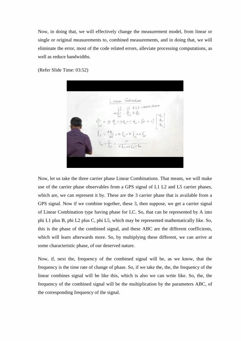
Now, let us take the three carrier phase Linear Combinations. That means, we will make

use of the carrier phase observables from a GPS signal of L1 L2 and L5 carrier phases,

which are, we can represent it by. These are the 3 carrier phase that is available from a

GPS signal. Now if we combine together, these 3, then suppose, we get a carrier signal

of Linear Combination type having phase for LC. So, that can be represented by A into

phi L1 plus B, phi L2 plus C, phi L5, which may be represented mathematically like. So,

this is the phase of the combined signal, and these ABC are the different coefficients,

which will learn afterwards more. So, by multiplying these different, we can arrive at

some characteristic phase, of our deserved nature.

Now, if, next the, frequency of the combined signal will be, as we know, that the

frequency is the time rate of change of phase. So, if we take the, the, the frequency of the

linear combines signal will be like this, which is also we can write like. So, the, the

frequency of the combined signal will be the multiplication by the parameters ABC, of

the corresponding frequency of the signal.

Now, the wavelength of the combined signal, as we know, wavelength is equal to C by

F; that means, the wavelength of the combines signal will be equal to, this. Now through

algebraic manipulation, we can get it. Now frequency of this is equal to, A into FL 1 plus

C into FL 5.


So, our, will be equal to, we can write it like this, C. Now you know this C is different

from, this is the constant C. And this is the velocity of the light. So, that distinction is to

be done. Now from this, we get A into lambda, L2 lambda, L5 plus B into lambda, L1

lambda, L5 plus C into lambda, L1 lambda, L2. And well get, lambda L1, lambda L2,

lambda L5. So, this is what is the wavelength of the combined signal.

And next all, what will be the integer ambiguity, of the combined signal; now we know

integer ambiguity is nothing, but phase by lambda. So, integer ambiguity of the

combined signal will be equal to, phase of the combined signal, divided by the

wavelength of the combined signal, though we know the phase of the combined signal is

summation of the individual signal, multiplied by the constants, divided by lambda LC.

So, if we now, we have to make some algebraic manipulation. So, for this, I can write

these things, by algebraic manipulation. Similarly, B into phi L2 lambda L2 plus C into,

this is what we can get from here.

Now, you can see, this is a constant. Because this is the wavelength of the L1 signal, this

is the wavelength of the linearly combined (Refer Time: 10:25) signal, and A is also

constant. So, all together this is a constant, say it is I, and here, this factor is nothing, but

it is the integer ambiguity of the signal L1, so phi by L1. So, integer ambiguity of the L1

signal, similarly this is another constant, J suppose, and this is the integer ambiguity of

the L2 signal, and this is (Refer Time: 10:52) constant K, the integer ambiguity of the L5

signal.

So, we see that the integer ambiguity of the combined signal is a summation of integer

ambiguity of the individual signal, multiplied by some constants. These constants are

again depending upon the, wavelength of these signals, as well as wavelength of the

combined signal, and a factor A. So, in this way, we can find out, we can get the

different characteristics, of the combined signal, which really provides us an insight, into

the nature of the combined signal.

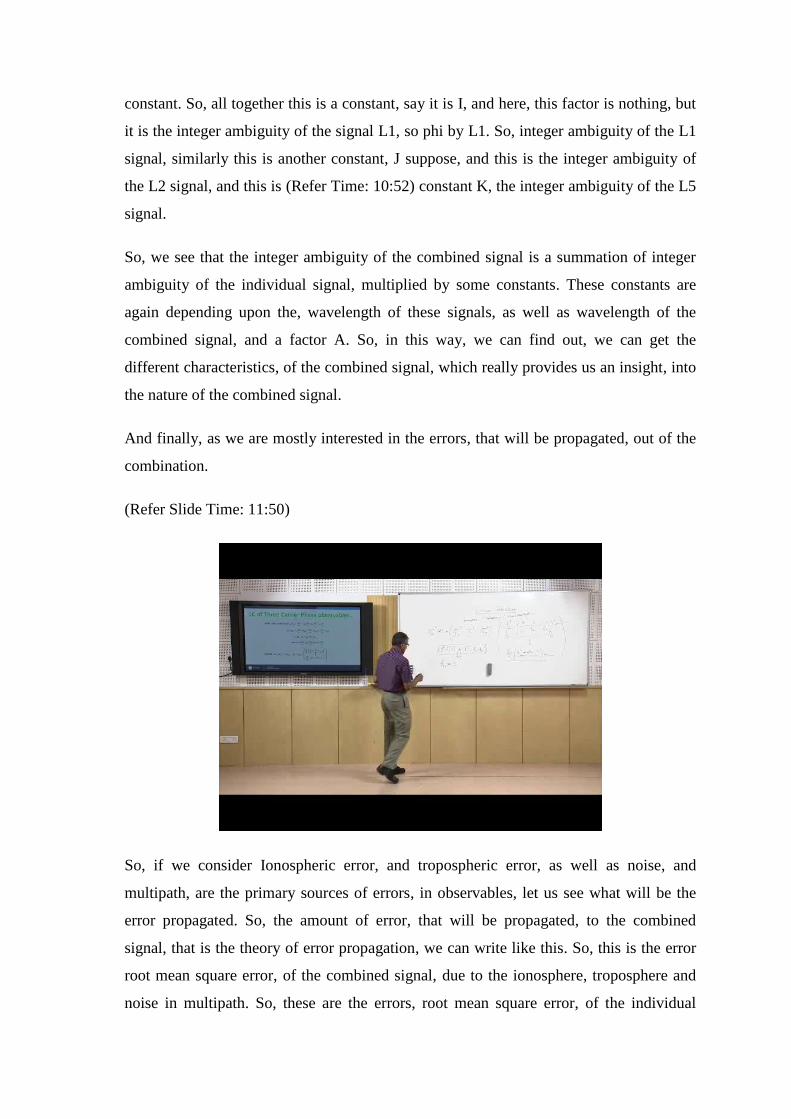
And finally, as we are mostly interested in the errors, that will be propagated, out of the

combination.


So, if we consider Ionospheric error, and tropospheric error, as well as noise, and

multipath, are the primary sources of errors, in observables, let us see what will be the

error propagated. So, the amount of error, that will be propagated, to the combined

signal, that is the theory of error propagation, we can write like this. So, this is the error

root mean square error, of the combined signal, due to the ionosphere, troposphere and

noise in multipath. So, these are the errors, root mean square error, of the individual

signal L1, L1 signal in the Ionospheric error, tropospheric error, this is the noise of

multipath error.

So, our errors will be defined in terms of the error that is associated with the L1 signal,

which is the most prominent signal, and this is multiplied by. And this, that means, this

multiplied, by this, will be the amount of Ionospheric error, in the combined signal. And

this multiplied by this; that means, this is what is the error in the tropospheric signal, and

your. So, and this multiplied by this, is the error due to noise.

Now we can see that, we can found that the errors associated with the, linearly combined

signal is the weight, these are the weights, weighted some of the errors that is associated

with the Ionospheric error, tropospheric error, and noise and multipath. And these

weights, you can see these weights, are primarily dependent on the coefficients ABC,

and the nominal frequency FL1 FL2 FL5. So, these are the prominent thing on which the

error will depend. And since the amount of error, is the weighted some of these weights,

weighted sum. So, these weights are called the amplification factor of errors. Because

depending upon these weights, the error gets amplified, or reduced as the combined

signal.

Now, if we can make this as 0, then our, this multiplied by this error with 0. So, our

Ionospheric error will be 0. So, the condition for Ionospheric error to be reduced to 0, or

nullify, is to make these 0. Now and to make the tropospheric error, to nullify,

tropospheric error, we get to make this character 0. Similarly now we can see here, all

these parameters A square plus B square plus C square. Under all circumstances,

whatever we take the value, of ABC, this summation will be always a positive number;

this indicates that, the error due to noise or multipath will always, increase, in case of

Linear Combination.

Now, as we know that the observables are different in different campaigns. So and so,

the errors, that will be associated with the GPS observables. Thus the constants, ABC,

we take; also well vary from campaign to campaign, to arrive at a particular

characteristics of the combined signal. Now, how to decide the value of ABC? The

criteria for deciding the value of ABC is to make this combined error should be

minimum. Because this is the primary objective, of our Linear Combination is to remove

or minimize the error, associated with the linearly combined signal. So, we have to make

this expression to be minimum, or in some cases because many times we may not make

minimize. So, it should be guided that, the errors due to ionosphere and troposphere as

well as noise should be minimum; it should be less in linearly combined signal, than that

is available in only L1 signal.

Actually the amount of error that will be associated with the linearly combined signal

will depend upon the, baseline length of the GPS observable, and the amount of errors

that will be associated, or the mutual errors. That means, what are the errors in

ionosphere and troposphere multipath mutually available, inside the observables and as

well, as it will also depend upon, what is a degree of accuracy, a user want to be

associated with the observables. So, on these factors, the quality or the amount of errors

that will be available in linearly combined will depend; that means, we have to choose

the values of ABC.

With this, I will like to go for the next type of Linear Combination which is widely

prevalent in today’s scenario.


Nowadays the Linear Combination, known as Melbourne-Wubbena liner combination, is

most widely used for minimizing or for other pre-processing, operation towards GPS

processing, to minimize the error associated with the GPS observable.


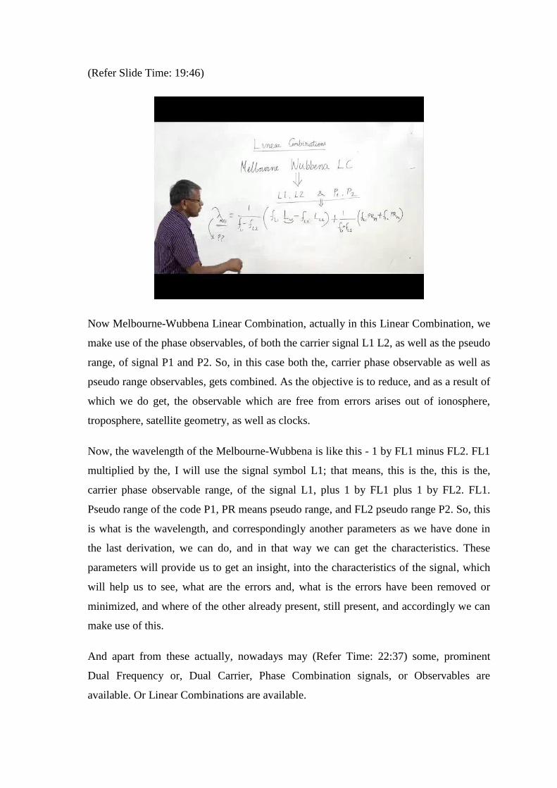
Now Melbourne-Wubbena Linear Combination, actually in this Linear Combination, we

make use of the phase observables, of both the carrier signal L1 L2, as well as the pseudo

range, of signal P1 and P2. So, in this case both the, carrier phase observable as well as

pseudo range observables, gets combined. As the objective is to reduce, and as a result of

which we do get, the observable which are free from errors arises out of ionosphere,

troposphere, satellite geometry, as well as clocks.

Now, the wavelength of the Melbourne-Wubbena is like this - 1 by FL1 minus FL2. FL1

multiplied by the, I will use the signal symbol L1; that means, this is the, this is the,

carrier phase observable range, of the signal L1, plus 1 by FL1 plus 1 by FL2. FL1.

Pseudo range of the code P1, PR means pseudo range, and FL2 pseudo range P2. So, this

is what is the wavelength, and correspondingly another parameters as we have done in

the last derivation, we can do, and in that way we can get the characteristics. These

parameters will provide us to get an insight, into the characteristics of the signal, which

will help us to see, what are the errors and, what is the errors have been removed or

minimized, and where of the other already present, still present, and accordingly we can

make use of this.

And apart from these actually, nowadays may (Refer Time: 22:37) some, prominent

Dual Frequency or, Dual Carrier, Phase Combination signals, or Observables are

available. Or Linear Combinations are available.


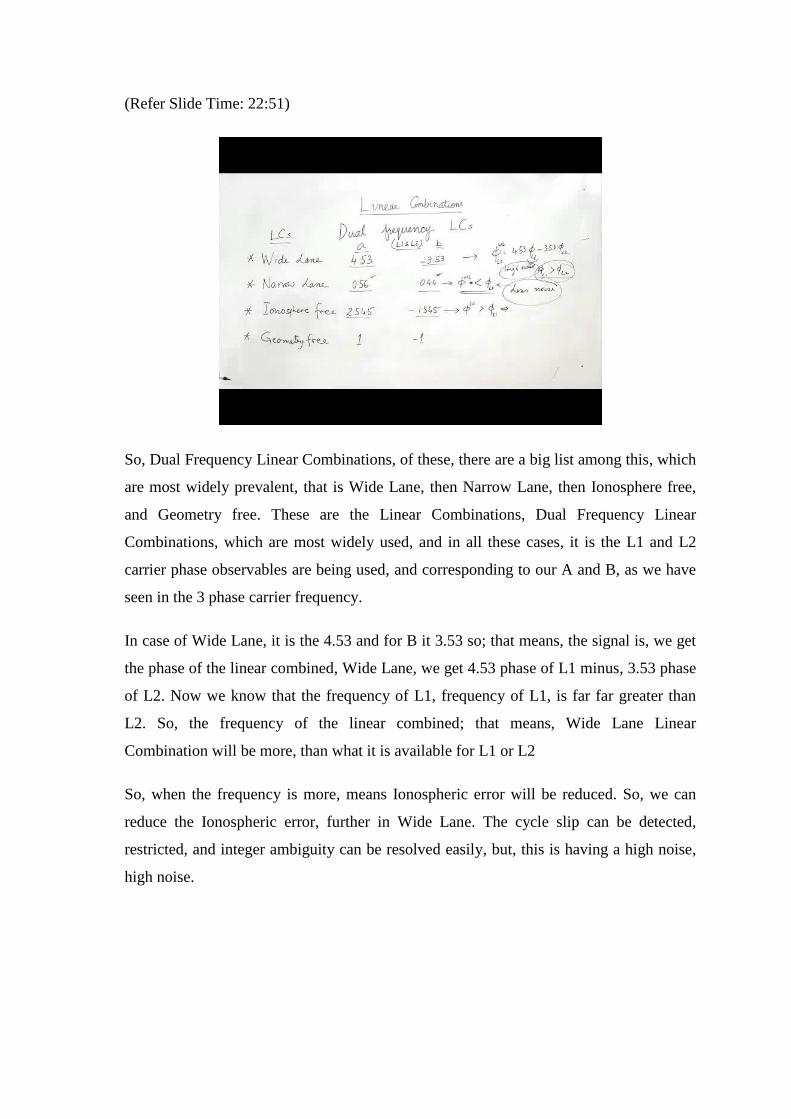
So, Dual Frequency Linear Combinations, of these, there are a big list among this, which

are most widely prevalent, that is Wide Lane, then Narrow Lane, then Ionosphere free,

and Geometry free. These are the Linear Combinations, Dual Frequency Linear

Combinations, which are most widely used, and in all these cases, it is the L1 and L2

carrier phase observables are being used, and corresponding to our A and B, as we have

seen in the 3 phase carrier frequency.

In case of Wide Lane, it is the 4.53 and for B it 3.53 so; that means, the signal is, we get

the phase of the linear combined, Wide Lane, we get 4.53 phase of L1 minus, 3.53 phase

of L2. Now we know that the frequency of L1, frequency of L1, is far far greater than

L2. So, the frequency of the linear combined; that means, Wide Lane Linear

Combination will be more, than what it is available for L1 or L2

So, when the frequency is more, means Ionospheric error will be reduced. So, we can

reduce the Ionospheric error, further in Wide Lane. The cycle slip can be detected,

restricted, and integer ambiguity can be resolved easily, but, this is having a high noise,

high noise.


So, noise is a embeddedments, and as a result, we will see, you see, that the errors are

very big. 5.76 meter.

So, now in case of Narrow Lane, we will make use of A is equal to 0.56, B equal to 0.44.

So, here though you can see, the Linear Combination, Narrow Lane; ultimately because

L1 frequency is more, L2 frequency is less. So, ultimately, we will see, that the

combined frequency will be less than, the frequency of this will be less than the

frequency of L1 single. So, frequency is less means, your Ionospheric error will be more,

but less noise. So, if we want to create a signal, which will be having less noise, then we

should make use of Narrow Lane concept, or an these constants we may use.

Then Ionosphere free linear combinations were 2. So, this is the constants which we have

to multiply, with the phase of the L1 signal, and phase of the L2 signals, and again, we

will find out, we will get frequency of Ionosphere free, will be more, than the frequency

of L1 signal. Which will provide us a good signal, for getting the Ionosphere free, we

will be able to compute the Ionospheric error easily, and we can make it free, and this

type of signal we design for baselines which are very long.

And Geometry free, where we get the signals having constant multiplied by 1 and minus

1. So, here also, will get a frequency, less than the frequency of the L1, and this will

provide us, a Geometry free signal, but it will have so many other errors. So, depending

upon the purpose, what for we are looking for, we want to pre-process the signal; we can

go for different types of linear sig combinations. And we can reduce, some of the

parameters we can enhance some of the parameters.


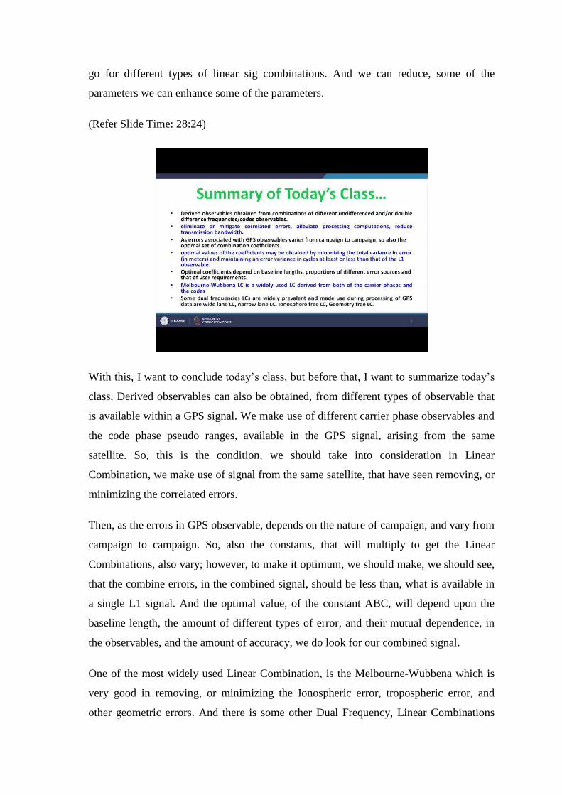
With this, I want to conclude today’s class, but before that, I want to summarize today’s

class. Derived observables can also be obtained, from different types of observable that

is available within a GPS signal. We make use of different carrier phase observables and

the code phase pseudo ranges, available in the GPS signal, arising from the same

satellite. So, this is the condition, we should take into consideration in Linear

Combination, we make use of signal from the same satellite, that have seen removing, or

minimizing the correlated errors.

Then, as the errors in GPS observable, depends on the nature of campaign, and vary from

campaign to campaign. So, also the constants, that will multiply to get the Linear

Combinations, also vary; however, to make it optimum, we should make, we should see,

that the combine errors, in the combined signal, should be less than, what is available in

a single L1 signal. And the optimal value, of the constant ABC, will depend upon the

baseline length, the amount of different types of error, and their mutual dependence, in

the observables, and the amount of accuracy, we do look for our combined signal.

One of the most widely used Linear Combination, is the Melbourne-Wubbena which is

very good in removing, or minimizing the Ionospheric error, tropospheric error, and

other geometric errors. And there is some other Dual Frequency, Linear Combinations

are available like, Wide Lane, Narrow Lane, Ionosphere free, Geometry free, etcetera,

which has their own characteristics, and depending upon the need, we can make use of

these different types of Linear Combinations, to serve our purpose particularly.

With this I would like to conclude, thank you. And see you, again, in the next class,

which will be on GPS processing, we will be talking on GPS processing in the next class.

Thank you.

gps surveying dr. jayanta kumar ghosh department of civil ... · indian institute of technology,...

Documents