gpgpu: general-purpose computation on...
TRANSCRIPT
2004
GPGPU: GPGPU: GeneralGeneral--Purpose Purpose
Computation on GPUsComputation on GPUsMark Harris
NVIDIA Developer Technology Group
The GPU has evolved into an extremely flexible and powerful processor
ProgrammabilityPrecisionPerformance
This talk addresses the basics of harnessing the GPU for general-purpose computation
Why GPGPU?Why GPGPU?

Motivation: Computational PowerMotivation: Computational Power
GPUs are fast…3 GHz Pentium 4 theoretical: 6 GFLOPS
5.96 GB/sec peak
GeForce FX 5900 observed*: 20 GFLOPs25.6 GB/sec peak
GeForce 6800 Ultra observed*: 40 GFLOPs35.2 GB/sec peak
*Observed on a synthetic benchmark: A long pixel shader with nothing but MUL instructions

GPU: high performance growthGPU: high performance growth
CPUAnnual growth ~1.5× decade growth ~ 60×Moore’s law
GPUAnnual growth > 2.0× decade growth > 1000×Much faster than Moore’s law
Why are GPUs getting faster so fast?Why are GPUs getting faster so fast?
Computational intensity Specialized nature of GPUs makes it easier to use additional transistors for computation not cache
EconomicsMulti-billion dollar video game market is a pressure cooker that drives innovation

Motivation: Flexible and preciseMotivation: Flexible and precise
Modern GPUs are programmableProgrammable pixel and vertex enginesHigh-level language support
Modern GPUs support high precision32-bit floating point throughout the pipelineHigh enough for many (not all) applications

Motivation: The Potential of GPGPUMotivation: The Potential of GPGPU
The performance and flexibility of GPUs makes them an attractive platform for general-purpose computation
Example applications (from www.GPGPU.org)Advanced Rendering: Global Illumination, Image-based Modeling Computational GeometryComputer VisionImage And Volume ProcessingScientific Computing: physically-based simulation, linear system solution, PDEsStream ProcessingDatabase queriesMonte Carlo Methods

The Problem: Difficult To UseThe Problem: Difficult To Use
GPUs are designed for and driven by graphicsProgramming model is unusual & tied to graphicsProgramming environment is tightly constrained
Underlying architectures are:Inherently parallelRapidly evolving (even in basic feature set!)Largely secret
Can’t simply “port” code written for the CPU!
Mapping Computational Mapping Computational Concepts to GPUsConcepts to GPUs
Remainder of the Talk:
Data Parallelism and Stream ProcessingComputational Resources InventoryCPU-GPU AnalogiesFlow Control TechniquesExamples and Future Directions

Importance of Data ParallelismImportance of Data Parallelism
GPUs are designed for graphicsHighly parallel tasks
GPUs process independent vertices & fragments
Temporary registers are zeroedNo shared or static dataNo read-modify-write buffers
Data-parallel processingGPU architecture is ALU-heavy
Multiple vertex & pixel pipelines, multiple ALUs per pipeHide memory latency (with more computation)

Arithmetic IntensityArithmetic Intensity
Arithmetic intensity = ops per word transferred
“Classic” Graphics pipelineVertex
BW: 1 triangle = 32 bytes OP: 100-500 f32-ops / triangle
Fragment BW: 1 fragment = 10 bytesOP: 300-1000 i8-ops/fragment
Courtesy of Pat Hanrahan

Data Streams & KernelsData Streams & Kernels
StreamsCollection of records requiring similar computation
Vertex positions, Voxels, FEM cells, etc.
Provide data parallelismKernels
Functions applied to each element in streamtransforms, PDE, …
Few dependencies between stream elementsEncourage high Arithmetic Intensity
Courtesy of Ian Buck
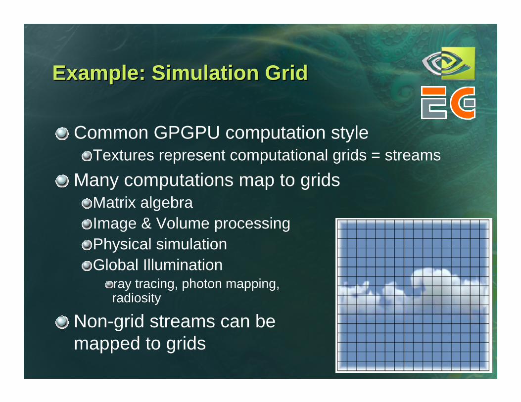
Example: Simulation GridExample: Simulation Grid
Common GPGPU computation styleTextures represent computational grids = streams
Many computations map to gridsMatrix algebraImage & Volume processingPhysical simulationGlobal Illumination
ray tracing, photon mapping, radiosity
Non-grid streams can be mapped to grids
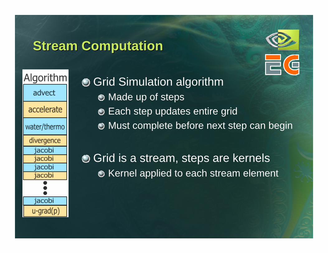
Stream ComputationStream Computation
Grid Simulation algorithmMade up of stepsEach step updates entire gridMust complete before next step can begin
Grid is a stream, steps are kernelsKernel applied to each stream element
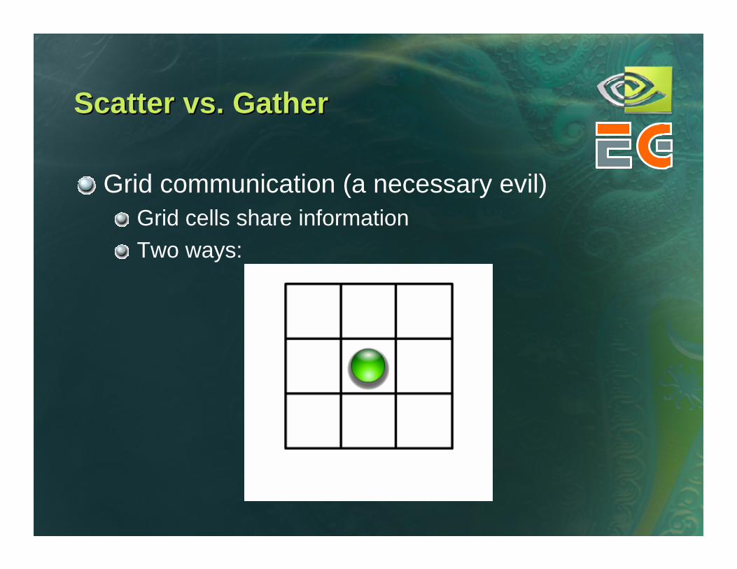
Scatter vs. GatherScatter vs. Gather
Grid communication (a necessary evil)Grid cells share informationTwo ways:
Computational Resources InventoryComputational Resources Inventory
Programmable parallel processorsVertex & Fragment pipelines
RasterizerMostly useful for interpolating addresses (texture coordinates) and per-vertex constants
Texture unitRead-only memory interface
Render to textureWrite-only memory interface
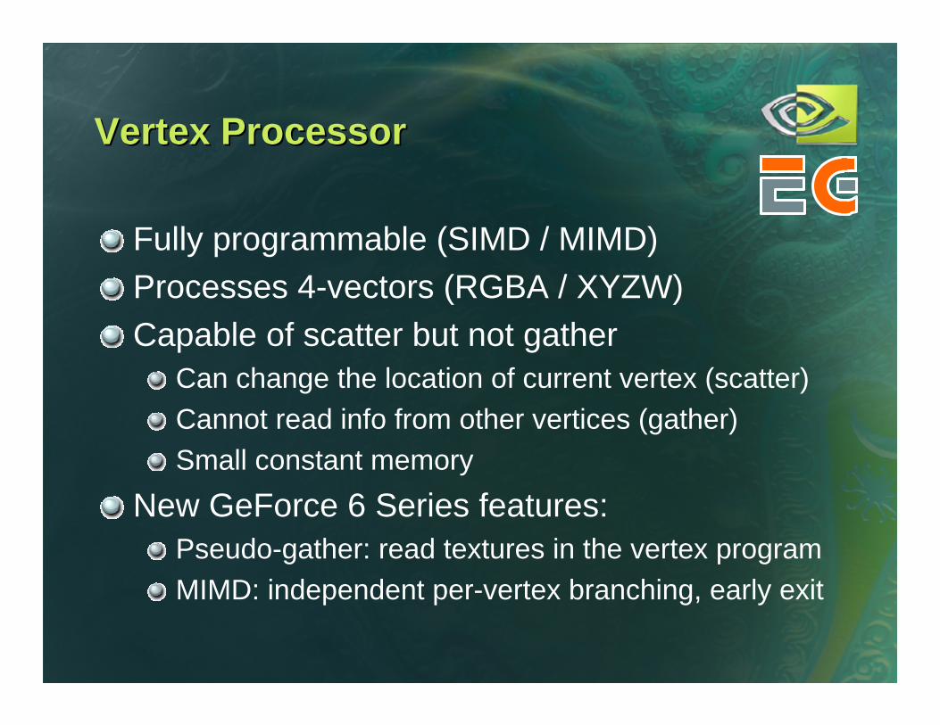
Vertex ProcessorVertex Processor
Fully programmable (SIMD / MIMD)Processes 4-vectors (RGBA / XYZW)Capable of scatter but not gather
Can change the location of current vertex (scatter)Cannot read info from other vertices (gather)Small constant memory
New GeForce 6 Series features: Pseudo-gather: read textures in the vertex programMIMD: independent per-vertex branching, early exit

Fragment ProcessorFragment Processor
Fully programmable (SIMD)Processes 4-vectors (RGBA / XYZW)Capable of gather but not scatter
Random access memory read (textures)Output address fixed to a specific pixel
Typically more useful than vertex processorMore fragment pipelines than vertex pipelinesGather / RAM readDirect output
GeForce 6 Series adds SIMD branchingGeForce FX only has conditional writes
CPUCPU--GPU AnalogiesGPU Analogies
CPU programming is (assumed) familiarGPU programming is graphics-centric
Analogies can aid understanding
CPUCPU--GPU AnalogiesGPU Analogies

GPU Simulation OverviewGPU Simulation Overview
Analogies lead to implementationAlgorithm steps are fragment programs
Computational kernels
Current state variables stored in texturesData streams
Feedback via render to texture
One question: How do we invoke computation?

Invoking ComputationInvoking Computation
Must invoke computation at each pixelJust draw geometry!Most common GPGPU invocation is a full-screen quad

Standard Standard ““GridGrid”” ComputationComputation
Initialize “view” (so that pixels:texels::1:1)glMatrixMode(GL_MODELVIEW);glLoadIdentity();glMatrixMode(GL_PROJECTION);glLoadIdentity();glOrtho(0, 1, 0, 1, 0, 1);glViewport(0, 0, gridResX, gridResY);
For each algorithm step:Activate render-to-textureSetup input textures, fragment programDraw a full-screen quad (1 unit x 1 unit)

ReactionReaction--DiffusionDiffusion
Gray-Scott reaction-diffusion model [Pearson 1993]Streams = two scalar chemical concentrationsKernel: just Diffusion and Reaction ops
∂U∂t
= Du∇2U −UV 2 + F (1−U ),
∂V∂t
= Dv∇2V +UV 2 − (F + k )V
U, V are chemical concentrations,F, k, Du, Dv are constants
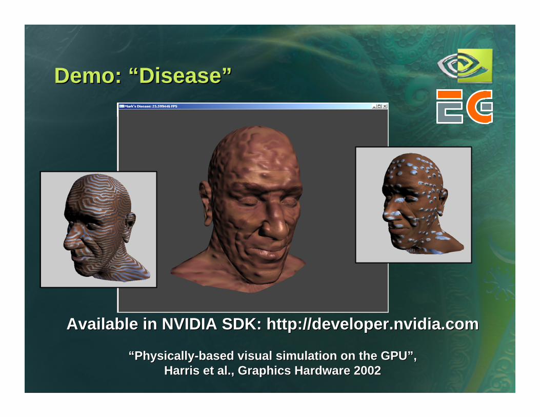
Demo: Demo: ““DiseaseDisease””
Available in NVIDIA SDK: Available in NVIDIA SDK: http://developer.nvidia.comhttp://developer.nvidia.com
““PhysicallyPhysically--based visual simulation on the GPUbased visual simulation on the GPU””,,Harris et al., Graphics Hardware 2002Harris et al., Graphics Hardware 2002

PerPer--Fragment Flow ControlFragment Flow Control
No true branching on GeForce FXSimulated with conditional writes: every instruction is executed, even in branches not taken
GeForce 6 Series has SIMD branchingLots of deep pixel pipelines many pixels in flightCoherent branching = likely performance winIncoherent branching = likely performance loss

Fragment Flow Control TechniquesFragment Flow Control Techniques
Try to move decisions up the pipelineReplace with mathOcclusion QueryDomain decompositionZ-cullPre-computation

Branching with Occlusion QueryBranching with Occlusion Query
OQ counts the number of fragments writtenUse it for iteration termination
Do { // outer loop on CPUBeginOcclusionQuery {
// Render with fragment program// that discards fragments that// satisfy termination criteria
} EndQuery} While query returns > 0
Can be used for subdivision techniques
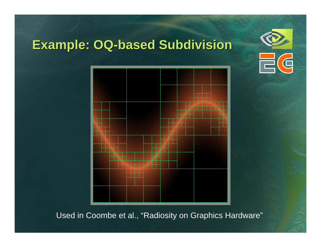
Example: OQExample: OQ--based Subdivisionbased Subdivision
Used in Coombe et al., “Radiosity on Graphics Hardware”
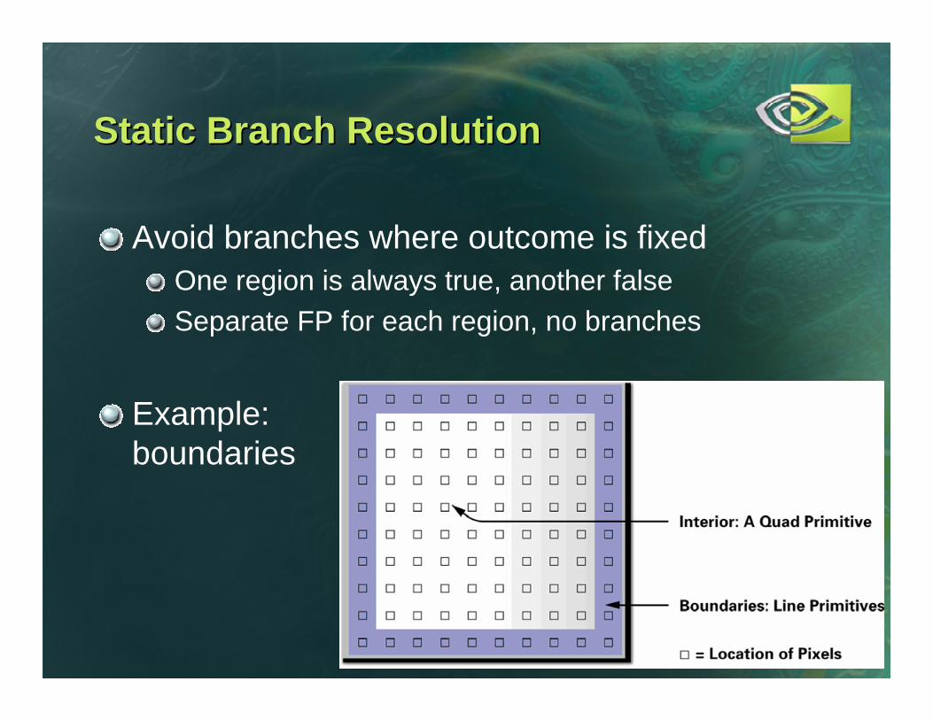
Static Branch ResolutionStatic Branch Resolution
Avoid branches where outcome is fixedOne region is always true, another falseSeparate FP for each region, no branches
Example: boundaries

ZZ--CullCull
In early pass, modify depth bufferClear Z to 1, enable depth testDraw quad at Z=0Discard pixels that should be modified in later passes
Subsequent passesEnable depth test (GL_LESS), disable depth writeDraw full-screen quad at z=0.5Only pixels with previous depth=1 will be processed
Can also use early stencil test on GeForce 6
PrePre--computationcomputation
Pre-compute anything that will not change every iteration!Example: arbitrary boundaries
When user draws boundaries, compute texture containing boundary info for cells
e.g. Offsets for applying PDE boundary conditionsReuse that texture until boundaries modifiedGeForce 6 Series: combine with Z-cull for higher performance!

GeForce 6 Series BranchingGeForce 6 Series Branching
True, SIMD branchingLots of incoherent branching can hurt performanceShould have coherent regions of > 1000 pixels
That is only about 30x30 pixels, so still very useable!
Don’t ignore overhead of branch instructionsBranching over only a few instructions not worth it
Use branching for early exit from loopsSave a lot of computation
GeForce 6 vertex branching is fully MIMDvery small overhead and no penalty for divergent branching
Current GPGPU LimitationsCurrent GPGPU Limitations
Programming is difficultLimited memory interfaceUsually “invert” algorithms (Scatter Gather)Not to mention that you have to use a graphics API…
Limitations of communication from GPU to CPUPCI-Express helps
GeForce 6 Quadro GPUs: 1.2 GB/s observedWill improve in the near future
Frame buffer read can cause pipeline flushAvoid frequent communication to CPU

Brook for GPUsBrook for GPUs
A step in the right directionMoving away from graphics APIs
Stream programming modelenforce data parallel computing: streamsencourage arithmetic intensity: kernels
C with stream extensionsCross compiler compiles to HLSL and CgGPU becomes a streaming coprocessor
See SIGGRAPH 2004 Paper andhttp://graphics.stanford.edu/projects/brookhttp://www.sourceforge.net/projects/brook

2004
ExamplesExamples

Example: Fluid SimulationExample: Fluid Simulation
Navier-Stokes fluid simulation on the GPUBased on Stam’s “Stable Fluids”Vorticity Confinement step
[Fedkiw et al., 2001]Interior obstacles
Without branching
Fast on latest GPUs~120 fps at 256x256 on GeForce 6800 Ultra
Available in NVIDIA SDK 8.0“Fast Fluid Dynamics Simulation on the
GPU”, Mark Harris. In GPU Gems.

Fluid DynamicsFluid Dynamics
Solution of Navier-Stokes flow equationsStable for arbitrary time steps[Stam 1999], [Fedkiw et al. 2001]
Fast on latest GPUs100+ fps at 256x256 on GeForce 6800 Ultra
See “Fast Fluid Dynamics Simulation on the GPU”
Harris, GPU Gems, 2004

Fluid Simulator DemoFluid Simulator Demo
Available in NVIDIA SDK: http://Available in NVIDIA SDK: http://developer.nvidia.comdeveloper.nvidia.com
Example: Particle SimulationExample: Particle Simulation
1 Million Particles1 Million ParticlesDemo by Simon GreenDemo by Simon Green
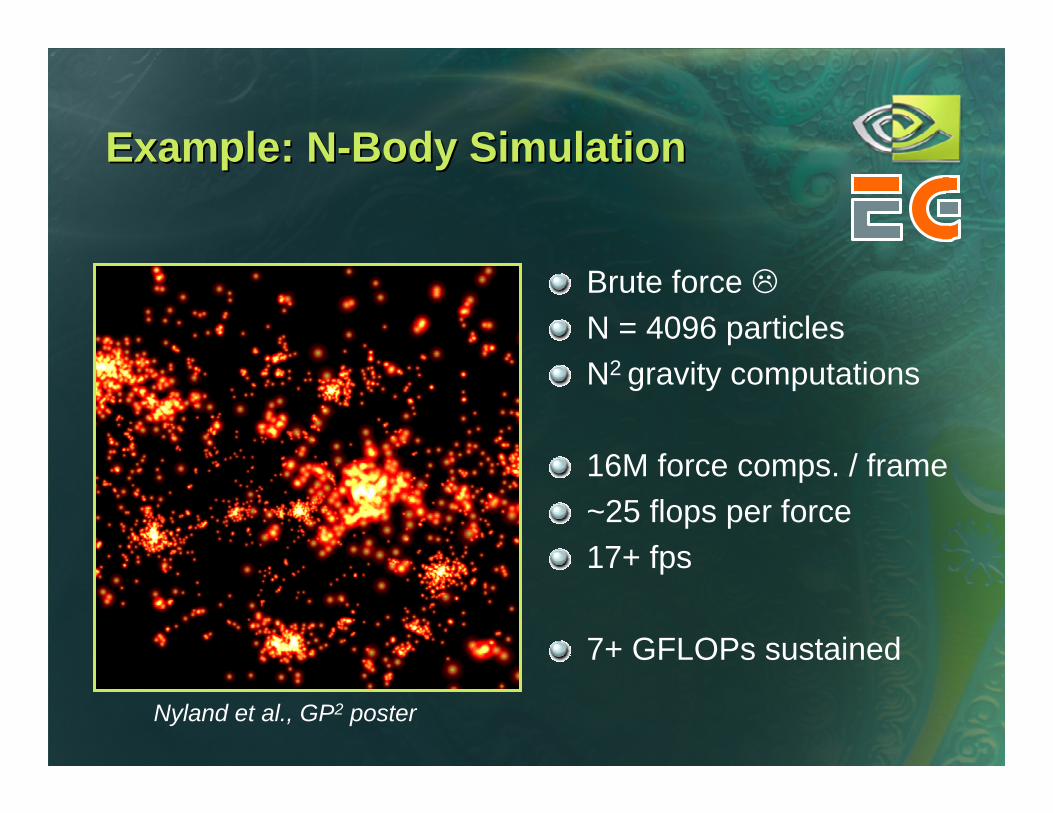
Example: NExample: N--Body SimulationBody Simulation
Brute force N = 4096 particlesN2 gravity computations
16M force comps. / frame~25 flops per force17+ fps
7+ GFLOPs sustained
Nyland et al., GP2 poster

The FutureThe Future
Increasing flexibilityAlways adding new featuresImproved vertex, fragment languages
Easier programmingNon-graphics APIs and languages?Brook for GPUs
http://graphics.stanford.edu/projects/brookgpu

The FutureThe Future
Increasing performanceMore vertex & fragment processorsMore flexible with better branching
GFLOPs, GFLOPs, GFLOPs!Fast approaching TFLOPs!Supercomputer on a chip
Start planning ways to use it!

More InformationMore Information
GPGPU news, research links and forumswww.GPGPU.org
developer.nvidia.org

New Functionality OverviewNew Functionality Overview
Vertex ProgramsVertex Textures: gatherMIMD processing: full-speed branching
Fragment ProgramsLooping, branching, subroutines, indexed input arrays, explicit texture LOD, facing register
Multiple Render TargetsMore outputs from a single shaderFewer passes, side effects

New Functionality OverviewNew Functionality Overview
VBO / PBO & SuperbuffersFeedback texture to vertex inputRender simulation output as geometryNot as flexible as vertex textures
No random access, no filtering
DemosPCI-Express
Higher GPU CPU bandwidth
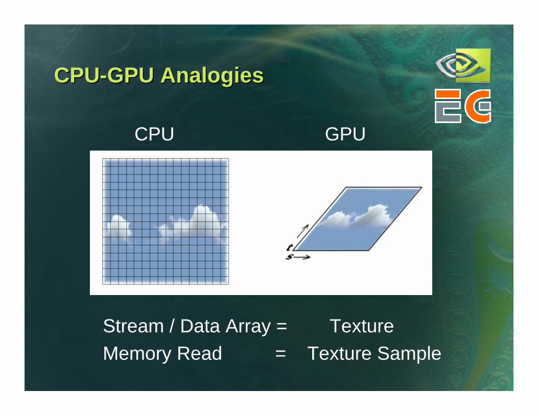
CPUCPU--GPU AnalogiesGPU Analogies
CPU GPU
Stream / Data Array = TextureMemory Read = Texture Sample

CPUCPU--GPU AnalogiesGPU Analogies
Loop body / kernel / algorithm step = Fragment Program
CPU GPU

FeedbackFeedback
Each algorithm step depend on the results of previous steps
Each time step depends on the results of the previous time step

CPUCPU--GPU AnalogiesGPU Analogies
.
..
Grid[i][j]= x;...
Array Write = Render to Texture
CPU GPU
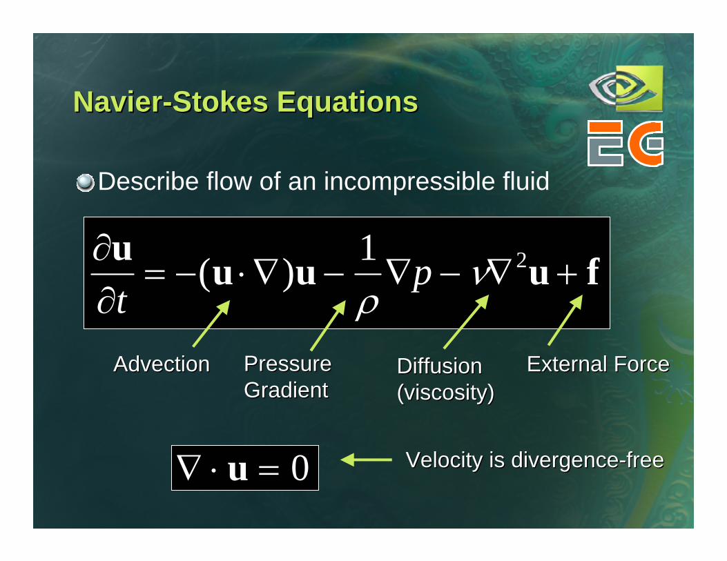
NavierNavier--Stokes EquationsStokes Equations
Describe flow of an incompressible fluid
∂u∂t
= −(u ⋅∇)u −1ρ∇p − ν∇2u + f
AdvectionAdvection PressurePressureGradientGradient
Diffusion Diffusion (viscosity)(viscosity)
External ForceExternal Force
∇ ⋅ u = 0 Velocity is divergenceVelocity is divergence--freefree
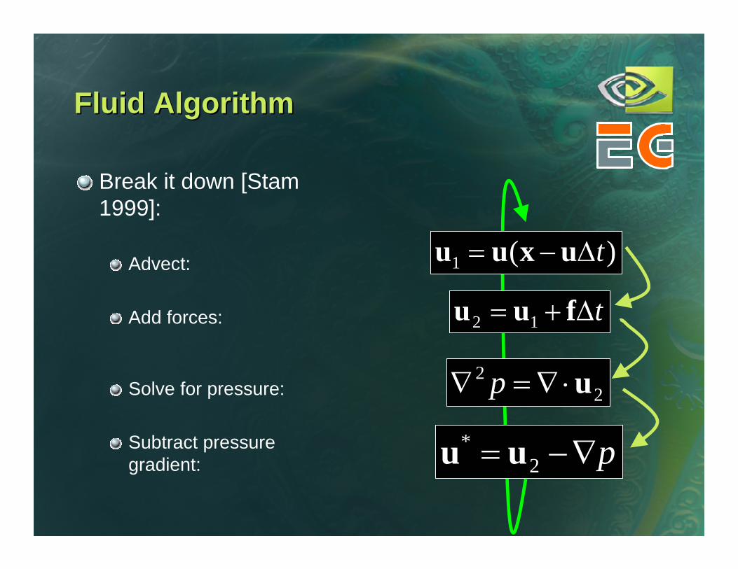
Fluid AlgorithmFluid Algorithm
Break it down [Stam1999]:
Advect:
Add forces:
Solve for pressure:
Subtract pressuregradient:
)(1 t∆−= uxuu
t∆+= fuu 12
22 u⋅∇=∇ p
p∇−= 2* uu

AdvectionAdvection
Advection: quantities in a fluid are carried along by velocity
Follow velocity field back in time from current position
uu((xx, , t+t+∆∆tt))
uu((xx’’, , tt))
Path of fluid
Trace back in time
float2 pos = coords – delta_t * tex(u, coords);
uNew = texBilerp(u, pos);
)(1 t∆−= uxuu

PoissonPoisson--Pressure SolutionPressure Solution
Discretize equation, solve using iterative solver Jacobi, multigrid, conjugate gradient, etc.Jacobi easy on GPU, but others possible tooDemo uses Jacobi iteration (50 iterations by default)
Compute divergence field, then repeatedly evaluate:
22 u⋅∇=∇ p
float pL = tex(pressure, coords + float2(-1, 0));float pR = tex(pressure, coords + float2( 1, 0));float pB = tex(pressure, coords + float2( 0,-1));float pT = tex(pressure, coords + float2( 0, 1));
float div = tex(divergence, coords);
pNew = 0.25 * (pL + pR + pB + pT – delta2 * div);