government statistician group list a topics · 2014-02-07 · the gss statistician competence...

Government Statistician Group List A Topics

January 2014

GSG List A Topic Guide

Contents Page

Introduction ........................................................................................................................... 2

1. Analysis of Variance (ANOVA) ....................................................................................... 4

2. Multiple Regression ....................................................................................................... 7

3. Other Multivariate Techniques ..................................................................................... 10

4. Stochastic Processes ................................................................................................... 14

5. Time Series Analysis ................................................................................................... 17

6. Generalised Linear Models .......................................................................................... 22

7. Hypothesis Testing ...................................................................................................... 26

8. Index Numbers ............................................................................................................ 31

Acknowledgements

We would like to thank the Department for Environment, Food and Rural Affairs, the Office for National Statistics and York University for their contributions to this material.


Introduction 3

Introduction

The GSS Statistician Competence Framework was updated and re-launched in June 2012. It stipulates that for admission to the Government Statistician Group (GSG), or for promotion to Grade 7, candidates must demonstrate a certain level of statistical analytical knowledge in a range of techniques. For entrance to the GSG, candidates must demonstrate knowledge in two statistical techniques from List A; for promotion to Grade 7, candidates should be able to demonstrate competence in at least three.

List A: Statistical Techniques for data analysis required for admission to or promotion within the GSG

1. Analysis of Variance: any of ANOVA, MANOVA, ANCOVA, MANCOVA; 2. Multiple Regression: either time-series or cross-sectional or both; 3. Other Multivariate techniques: any of Principle Component Analysis, Factor Analysis,

Clustering techniques, Discriminant Analysis; 4. Stochastic Processes: including for example, Markov chains, Queuing Processes,

Poisson processes, random walks; 5. Time Series Analysis: any of Time Series models, ARIMA processes and

Stationarity, Frequency Domains Analysis; 6. Generalised Linear Models: any of Log-Linear models, Logistic Regression, Probit

Models, Poisson Regression; 7. Hypothesis Testing: all of formulation of hypotheses, types of error, p-values,

common parametric (z, t, F) or non-parametric (Χ2, Mann-Whitney U, Wilcoxon, Kolmogorov-Smirnov) tests

8. Index Numbers: most of Laspayres/Paasche indices, hedonic indices, chaining, arithmetic and geometric means as applied to indices.

This booklet aims to provide an overview and some technical detail of the eight listed statistical techniques to aid with refreshing your statistical knowledge. If further training is required, the Statistical Training Unit at the ONS currently offers short courses (half day or one day) in: ANOVA, Multiple Regression, Probit/Logistic Regression, Generalised Linear Models, Hypothesis Testing, Index Numbers and Time Series. If you are interested in attending one of these, please email [email protected].

mailto:[email protected]�


Analysis of Variance (ANOVA) 4

1. Analysis of Variance (ANOVA)

1.1 Introduction

ANOVA is used to test the hypothesis that the means of two or more independent (i.e. unrelated) groups are (all) the same. This technique is an extension of the t-test, and is typically used when there are more than two groups to test.

The logic of using ANOVA to test for differences as opposed to multiple t-tests between all pairs of groups is that when conducting a t-test there is a chance of making a Type I error which happens when a test finds a significant difference between means, when one does not exist. Typically this error rate is five per cent, however, the chances of making a Type I error increases with the number of t-tests run. An ANOVA test controls for these errors so that the Type I error rate remains constant throughout the test , giving confidence that any significant result found is not just down to chance.

ANOVA is a parametric test which relies on certain assumptions (see below). When these are violated, the non-parametric equivalent of ANOVA - the Kruskall-Wallis test, may be used in its place.

1.2 When should this technique be used?

You should use ANOVA when:

a you want to test the effect of different conditions or treatments on the outcome or response of the same dependant variable, between different groups whose members have been randomly assigned to each group from one larger group. Each subject is allocated to one, and only one, group.

b you want to test the effect of different conditions or treatments on the outcome or response of the same dependant variable between different groups that are split based on some independent variable. Again, each member will be assigned to one group only.

1.3 Technique Detail

Primarily ANOVA will determine that differences exist among means. The null hypothesis in an ANOVA test is that (all) the group means are the same, for example:

0 1 2 3H : ... Gµ µ µ µ= = = =

whereas the alternative hypothesis is that there are at least two group means that are significantly different from each other.

The underlying model (determined by the set-up/details of the experiment) should be stated explicitly. For the most basic model, the one-way ANOVA, and an extension of the t-test, that model would be:

Observation = Overall mean effect + Effect for Group g + Error term

Note: more extensive experience of ANOVA leads to knowledge of more complex models and designs. Terms encountered may include two-way crossed, two-way crossed with



interaction and replication, three-way (etc.); nested and hierarchical models (in contrast to the crossed models); and fixed effects and random effects.

At its most basic, ANOVA compares the variation of individual scores between groups (group means) to the variation of individual scores within the groups.

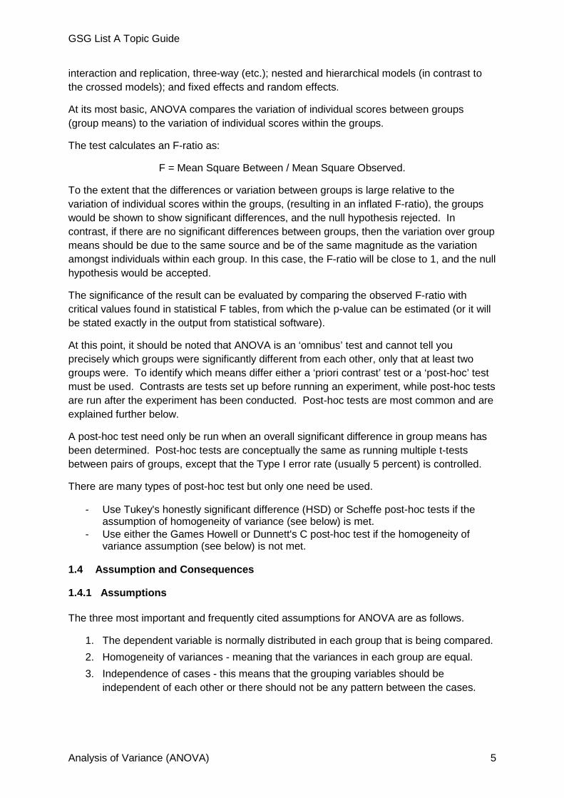
The test calculates an F-ratio as:

F = Mean Square Between / Mean Square Observed.

To the extent that the differences or variation between groups is large relative to the variation of individual scores within the groups, (resulting in an inflated F-ratio), the groups would be shown to show significant differences, and the null hypothesis rejected. In contrast, if there are no significant differences between groups, then the variation over group means should be due to the same source and be of the same magnitude as the variation amongst individuals within each group. In this case, the F-ratio will be close to 1, and the null hypothesis would be accepted.

The significance of the result can be evaluated by comparing the observed F-ratio with critical values found in statistical F tables, from which the p-value can be estimated (or it will be stated exactly in the output from statistical software).

At this point, it should be noted that ANOVA is an ‘omnibus’ test and cannot tell you precisely which groups were significantly different from each other, only that at least two groups were. To identify which means differ either a ‘priori contrast’ test or a ‘post-hoc’ test must be used. Contrasts are tests set up before running an experiment, while post-hoc tests are run after the experiment has been conducted. Post-hoc tests are most common and are explained further below.

A post-hoc test need only be run when an overall significant difference in group means has been determined. Post-hoc tests are conceptually the same as running multiple t-tests between pairs of groups, except that the Type I error rate (usually 5 percent) is controlled.

There are many types of post-hoc test but only one need be used.

- Use Tukey's honestly significant difference (HSD) or Scheffe post-hoc tests if the assumption of homogeneity of variance (see below) is met.

- Use either the Games Howell or Dunnett's C post-hoc test if the homogeneity of variance assumption (see below) is not met.

1.4 Assumption and Consequences

1.4.1 Assumptions

The three most important and frequently cited assumptions for ANOVA are as follows.

1. The dependent variable is normally distributed in each group that is being compared. 2. Homogeneity of variances - meaning that the variances in each group are equal. 3. Independence of cases - this means that the grouping variables should be

independent of each other or there should not be any pattern between the cases.



1.4.2 Consequences

The consequences and methods to resolve assumptions are as follows.

1. ANOVA can handle data that is non-normal with only a small affect on the Type I error rate. However this can be more problematic when group sizes are small. There are two methods of dealing with the problem of non-normal data: a) transform the data using various algorithms so that the shape of the distribution becomes normally distributed; b) choose the non-parametric equivalent test mentioned in the introduction.

2. For violation of the second assumption it is possible to run a Welch test. The Welch statistic tests for the equality of group means. This statistic is preferable when the assumption of equal variances does not hold.

3. A lack of independence of cases has been stated as the most important assumptions to fail. Often, there is little you can do that offers a good solution to this problem.

1.5 Practical Applications

ANOVA is a commonly used research technique in business, medicine, psychology and ecology. For example in business, ANOVA could be used to determine significant differences between sales in different areas; in Psychology ANOVA could be used to compare the behaviour patterns of different groups of people; in medicine ANOVA can be used to detect differences in the effectiveness of different drugs; while in ecology it could be used to detect differences in landscape response to the use of different grazing patterns.

1.6 Further Information

Wikipedia has an excellent entry on ANOVA available at the following address: http://en.wikipedia.org/wiki/Analysis_of_variance

1.7 Relevant Software

ANOVA can be run using: SAS using proc ANOVA or proc GLM; SPSS using the Compare Means function; MINITAB; R; Excel 2007 and later versions, using the Data Analysis tool in the Data menu.

http://en.wikipedia.org/wiki/Analysis_of_variance�


Multiple Regression 7

2. Multiple Regression

2.1 2.1 Introduction

Regression is about fitting models (including lines, curves, multi-dimensional lines / planes, etc.) to observed data, which can then be used to help inform interpretation and predict responses given a set of explanatory values. Fitting of lines involves choosing models that define one response variable, y, in terms of one or more independent variables, x, and a model/relationship given in terms of a set of parameters, the values of which are to be estimated. The observed data (y, x) are known, and usually assumed to be fixed (i.e. non-random). We first note some distinctions in regression model terminology:

- Simple linear regression: the ‘classic’ case of only one independent variable, and a straight-line relationship with the response: 0 1y xβ β= + . The error-term is assumed additive, and to come from a normal distribution with mean zero and constant variance.

- Multiple linear regression: an extension of the above case, but the model still retains the form ( ; )i i iy f ε= +xβ , where the function f is linear in the parameters

0 1

1

0 1 1 2 22

0 1 2

y xy xy x x

y x x

β βββ β β

β β β

= +

=

= + +

= + +

but need not be linear in the x’s. The following are all examples of functions that are linear in the parameters:

We still assume an additive error term, which is normally distributed with mean zero. However, its variance need not be constant (for example, the error variance may be assumed to be proportional to x), and a weighted model can be fitted.

- Non-linear regression is the term used to apply to models that are not linear in the parameters. An example of a such a function is 1

0 xy eββ= . Some models, like the example, can be made linear by applying a suitable transformation:

*0 1 1ln( ) ln( ) oy x xβ β β β= + = + ,

following which the linear theory (if we assume the error term is additive in the transformed model) can be applied.

The basis of the underpinning method for linear regression is least squares, in which the parameter estimates minimise the sum of squares of the error terms (ESS):

. 2 2

1 1ESS ( ( ; ))

n n

i i ii i

y fε= =

= = −∑ ∑ xβ

Multiple regression formalises this into statistical theory and allows multiple dimensions to the graph and finds a multi-dimensional line of best fit.


Use multiple regression when:

- you have a specific variable you wish to investigate,

- the variable does not depend on its previous levels,



- you want to establish the scale and statistical significance of correlations,

- you want to predict a response based on values of explanatory variables,

- you want to find the effect of an explanatory variable after controlling for differences in other variables.


Step1: Decide upon your response variable. This must be the key thing that you wish to investigate. You may need to construct or transform it so that the key questions you have can be applied directly to it.

Step2: Identify the explanatory variables that you want to include. Decide for each whether to split it into bands/groupings or to treat it as a linear relationship. Using bands is more robust but linear is more powerful. Also need to decide whether functions of variables need to be included, e.g. in modelling earnings (which flattens out with age), may need to include both Age and Age2 variables in the model. Dummy variables may need to be set up for the handling of discrete/banded/categorical variables.

Step 3: Compose the model. You have to choose which explanatory variables to include in the model depending on the amount they improve the fit of the model. The interaction between variables needs to be checked. Selecting variables to be included in the model can be done using a stepwise approach (forwards and backwards) and by checking the significance of the parameters and amount of variation explained by a parameter.

Step 4: Check for outliers by identifying the largest residuals (where data point has large deviation from the fitted point). If one or a few appear to be much larger than others then check the data underlying these points and consider their removal from the analysis if you think they are unreliable or unrepresentative. Refit the model without these points.

Step 5: Check that the residuals come from a random Normal distribution. Most software has residual plots that can reveal deviation from normality.

Step 6: Identify which data points have the most influence on the model using, for example, plots of Cook’s distance. Decide if you are happy that the model is sensitive to this data. Explain this sensitivity when presenting the results.

Step 7: The model will not be perfect. Decide if you can live with the model despite its failings. If you don’t want to predict a response variable or quote standard errors then you may be happy with a poor fitting model which is still averaging the data.

Step 8: Interpret the output. This should be done throughout while building the model, but there is a need to understand and interpret the ANOVA tables and other summary statistics produced by software. These include a measure of the variability in the data explained by the model, significance of the model and its parameters, as well as interpreting the parameter estimates themselves.



2.4 Assumptions and consequences

2.4.1 Assumptions

a Independence of data points.

b Residuals (the difference between the actual data points and the best fit line) have a Normal distribution.

c No multi-colinearity.

No serial correlation or autocorrelation. I.e. the response variable should not depend on its previous levels but only on the explanatory variables.

2.4.1 Consequences

a The approach is not the right one to use.

b Standard errors will not be statistically reliable. Try adding more explanatory variables. Try transforming the dependent variable by taking logs perhaps.

c Several parameters will operate in combination with individual levels being wild. Standard errors will be very large indicating unreliable estimates.

Standard errors will not be statistically reliable and the goodness of fit may be optimistic. (Need to use a time series analysis.)


Used with Family Food data to estimate the association between income and fruit purchases after controlling for differences in region, household composition, age of household reference person, ethnic origin of household reference person.


Wikipedia, software manuals


All statistical packages including SAS, SPSS, and R. Spreadsheets can be used with caution, but are not a good interface to keep track of your model as it develops.


Other Multivariate Techniques 10

3. Other Multivariate Techniques

3.1 Introduction

The word multivariate could describe any statistical method based on more than one observed variable, including correlation, cross tabulation, and regression among others. Although some textbooks use multivariate in this sense, it is more common to apply a more restricted definition. These notes will concentrate on methods for simplifying or finding patterns in large datasets containing multiple measurements of each observed object (person, animal, plant, town, etc). There are many such methods, including: Multiple ANOVA (MANOVA), Multivariate Regression, Principal Component Analysis, Factor Analysis, Discriminant Analysis and Cluster Analysis. As expressed by Vic Barnett (Interpreting Multivariate Data, 1980), “The emphasis is on exploring the data, rather than on subjecting them to models and procedures based often more on [mathematical] convenience than relevance.” We want to extract information and meaning from what otherwise might be uncommunicative data.


Sometimes multivariate analysis may be the main focus of a particular piece of work, perhaps because the objective is to explore relationships between the variables in a dataset. However, more commonly it can be used in addition to other approaches, such as formal models in the case of scientific data, or tabulation of government survey data. The multivariate analysis may take place after the main analysis, for example where a tight timetable restricts what can be done prior to publication of a stats notice. Alternatively, use of multivariate techniques at an earlier stage is frequently beneficial in order to suggest important relationships to explore in the main analysis.


3.3.1 Data requirements

Data for analysis usually need to be formed as a table, the columns forming ‘variables’ and the row forming ‘units of analysis’. The unit of analysis does not have to correspond to the ‘unit of observation’ or the ‘sampling unit’.

Variables may be continuous or discrete. Discrete values may be natural (eg counts) or arbitrary codes that may be ordered or purely nominal. Analysing multivariate data often includes tasks to recode or transform values, and to select or weight cases. It is important to ensure that coded categorical data is appropriately handled and not treated as if it were a continuous variable. Another data restructuring worth knowing about is to switch time-series data between ‘wide form’, where observations of each unit at different times are stored in separate columns, and ‘long form’, where the time value forms one variable and the observation is a second variable. Each row in the long form is identified by a unit/time combination. The exact data requirements will depend upon the technique being used, and, naturally, should be well-understood before attempting to use it.

Multivariate data very commonly contains ‘missing values’, which may be accidental or structural. Various methods allow for missing data, either by exclusion or imputation. The impact of the missing data in a particular dataset needs to be understood. For example, a



few values missing-at-random may be accommodated by excluding units, but greater numbers will demand more complex approaches. The choice of codes to mark missing values and whether software marks these as missing and supplies a default handling mechanism are also essential knowledge for the analyst. A sensitivity analysis may be needed.

3.3.2 Exploratory analyses

Before using any complex statistical analysis method, it is sensible to explore the data using simple univariate statistics (means, medians, quantiles, etc.) and histograms to reveal the shape of distributions. A starting point for multivariate analysis is often a ‘scatterplot matrix’, where each variable is plotted against every other. Where there is some natural grouping to the data (e.g. rural/urban, types of farm, etc.) different colours/symbols can be used in scatterplots, or the grouping factor can be used to classify table. All these approaches help to develop the statistician’s understanding of the data, and also highlight outliers, including those resulting from recording errors.

3.3.3 Techniques

In this section we provide a few comments about some of the main techniques used.

(a) Principal Components Analysis (PCA):

- From p original variables, create at most p new variables (the principal components (PCs)) that contain most of the information from the original variables. In this sense, the dimensionality of the data set can be reduced (leaving fewer variables to work with) whilst retaining most of the information it contains.

- The PCs are uncorrelated (orthogonal), thus avoiding multi-collinearity, which can be problematic if the original variables were to be used in other techniques (eg regression). As a visualisation, if two variables are considered, PCA rotates the axes so that the new variables – the PCs – have zero correlation.

- The PCs are created as linear combinations of the original variables, X:

1 11 1 1

1

...... ... ... ... ...

...

p

p p pp p

PC a a X

PC a a X

=

where the coefficients a are to be determined.

- Initially, p PCs are created, ordered by descending variance, and only the first q <= p will be retained; those not retained will be the ones that contribute least to the overall variability. A scree plot can be used to help decide the cut-point.

- The method behind PCA uses either the variance-covariance matrix, S, of the variables, or the correlation matrix, R; the user chooses which is more appropriate for the particular application. The PCs’ variances, the coefficients for the equations, and then new data set values are derived via determination of the eigenvectors of S or R – of course, statistical software would usually be used for this purpose.

- The outputs can then be used in further analysis, and interpretation of what the PCs mean (i.e. which original variables they mainly comprise) is useful.

- We note that PCA is closely related to Factor Analysis.



(b) Cluster Analysis

- The aim of cluster analysis is to put the individual subjects into some grouping or classification based upon the subjects’ similarity/dissimilarity with each other.

- No grouping structure is provided beforehand.

- There are various metrics that can be used to define similarity/dissimilarity between all pairs of clusters/observations. A common one is the Euclidean distance, and standardising each variable first is usual to avoid variables that have great variance from dominating.

- There are various algorithms for carrying out the clustering. K-means, which allows the number of clusters to be defined beforehand is one common method. Another method is (agglomerative) hierarchical, in which the cases are initially treated as n clusters of 1 observation, and are iteratively grouped together to finally give 1 cluster of n observations. A dendrogram, with appropriate cut-off, can help determine a suitable grouping/clustering structure.

- The method is suitable for most data types (including continuous, discrete, binary, categorical, ordinal) though some transformation work may be required initially.

(c) Discriminant Function Analysis

- Data requirements are for (precisely) one categorical variable (ie an indicator showing to which category a subject belongs), and one or more predcitor variables.

- The aim is to develop a prediction as to what category a subject is most likely to belong, based upon his/her/its predictor variable values. For example, if a patient doesn’t smoke, likes eating chips, is not young, has high blood pressure … is (s)he more likely to have high or normal cholesterol?

- Fisher’s Linear Discriminant Function (LDF) determines a linear combination, a1X1 + a2X2 + …+ apXp of the original variables that can be used as a good predictor: subjects in the same group would have similar values of the linear combination, and those in a different group, would have different values. The solution is based on the ratio of between-to-within group variances, and is determined by an evaluation of eigenvectors. An individual would be classified based on the smallest distance between his/her/its LDF score and each group’s average score.

- An alternative approach is via classification functions, where the individual’s assignment is based upon the max score evaluated for each group. Various other methods also exist.

3.3.4 Data reduction

The problem of multivariate data is complexity. Many multidimensional analyses aim to demonstrate that the data can be analysed in fewer dimensions than initially presented, without substantial loss of information. It may be a matter of judgment what proportion of lost information is acceptable. Socio-economic analyses often rely upon dimensional reduction because they deal with fuzzy concepts for which there is no unique or direct measure. The classic example is intelligence, for which the IQ scale was derived by factor analysis of a battery of tests. A more agricultural example is the use of Principal Components Analysis to derive an overall measure of fertiliser use from multivariate information on the quantities of the different components used on farms.



3.4 Assumptions

Most multivariate analyses make no formal distributional assumptions, but many techniques are sensitive to outliers and skewed distributions, which is why exploratory analyses are important. Transformations are useful for skewed distributions.


Specialist software is needed for multivariate techniques but the major statistical packages all have the most commonly used techniques:

- SAS - SPSS - Stata - GenStat - R

Terminology may differ between packages and sometimes outputs are scaled differently.

Specialist programs are available for some techniques; either stand alone programs, such as DECORANA for detrended correspondence analysis, or add-in packages to extend R.


Stochastic Processes 14

4. Stochastic Processes

4.1 Introduction

A stochastic process (often called a random process) is a family of indexed random variables that define the distribution of values at each value of the index, which is often a measure of time. Hence they are often used to represent a series of events or transitions over time. Rather than studying uncertainty or variation as a characteristic of populations, stochastic processes model it as a consequence of randomness determining the outcome of processes, which may evolve in multiple directions. The index or measure of time can take either discrete values or continuous values.


Most analysis of stochastic processes focuses on Markov chains, which have the property that future outcomes conditional on the current value are independent of the past. This property greatly simplifies definition of a Markov chain and allows generalisation. It also has various formal consequences, which allow simplification of analysis, trends and long term outcomes. Markov chains are often useful for analysis of models in which systems are treated as mechanistic, i.e. an analogy is made with a machine. More or less the simplest Markov chains are stationary processes, which can represent noise within a model of a time series. Renewal processes represent successive occurrences of events such as radioactive emissions, or machine failures. Random walks represent systems in which expected errors or distances can accumulate over time, while retaining a chance that the net error or distance can return to zero. Branching processes allow modelling and analysis of growth in generations. Where systems or elements in systems can be simplified to a finite set of alternative states, a Markov chain can be very simply and powerfully represented by a matrix that defines changes in a single time step. Finally, the Markov Chain Monte Carlo method has become a widely used process for ensuring that randomization methods for parameter estimation converge on valid parameter sets, although its explanation is beyond the scope of these notes.


The Markov property specifically allows change to be dependent on the value of the index variable, but introductions to stochastic processes usually focus on the ‘homogeneous’ special case, in which change is independent of the index variable. If the current state is defined as a vector of probabilities of each state, the matrix is a ‘state transition matrix’, or stochastic matrix, in which the sum of each row is unity (in a right hand matrix). Such a matrix can describe the dynamics of states with a fixed total, such as the proportions of different land covers within a region. In the more general case, in which the current state is a vector of frequencies, the matrix is termed a ‘population projection matrix’. These matrices can represent the demography of a population that is changing size. Presentations often focus on transition matrices, but projection matrices are almost as simple and have additional powerful applications. A state or set of states is ‘absorbing’ if there is zero probability of leaving that set of states. A Markov chain is ‘irreducible’ if all states can be reached from all alternative states in the chain. A dead state is usually avoided in stochastic process models, because it is an absorbing state that prevents the Markov chain from being irreducible. The period of each state in a stochastic process is the minimum number of time



steps required to return to it when starting from it. A process is ‘aperiodic’ if the maximum common divisor of the periods of states in the process = 1. This can be indicated by finding a power of the change matrix at which all its elements are strictly positive, i.e. real and greater than 0.

4.4 Assumptions and Consequences

4.4.1 Assumptions

- Markov property: Future outcomes of a stochastic process conditional on the current value are independent of the past.

- Irreducible: All states in the process can be reached from all alternative states.

- Homogeneous: Transitions are independent of the index variable (usually time).

- The values in the current state vector are probabilities or population sizes so they are non-negative. Therefore all elements in the change matrix are non-negative.

4.4.2 Consequences

The Markov property severely limits the dependence of the long term state of the process on its initial state.

1. If a process is a homogeneous, irreducible, aperiodic Markov chain with a state vector with sum =1, it will have a unique stationary distribution independent of its initial state, which is defined by a state vector that remains constant if the process continues.

2. If a process is a homogeneous, irreducible, aperiodic Markov chain with a state vector with sum <> 1, the dominant eigenvalue (largest in magnitude) is the potential intrinsic growth rate of the population when it reaches its stable demographic composition, which is defined by the eigenvector.

3. Periodic cases and cases with absorbing states.


Stochastic processes have a wide range of practical applications, particularly in economics (e.g. stock and exchange rate fluctuations), medicine (e.g. blood pressure and temperature data) and modelling signals such as speech and audio.

4.6 Sources of Further Information

Two very different textbooks stand out. Both have been reprinted multiple times.

A university text:

Geoffrey Grimmett and David Stirzaker (2001) Probability and Random Processes 3rd Edition. Oxford University Press.

A very influential book in quantitative ecology:

Hal Caswell (2001) Matrix Population Models 2nd Edition: Construction, Analysis and Interpretation. Sinauer.




The attraction of these methods is the ability to readily construct bespoke solutions to a wide range of problems. These problems also tend to be especially suitable for simple computer programming. However, various matrix problems are best solved using sophisticated numeric methods. Hence high level programming languages with access to libraries of matrix functions and solutions are most suitable, such as:

R, Matlab, Maple or Mathematica.


Time Series Analysis 17

5. Time Series Analysis

5.1 Introduction

A time series is a sequence of measurements in time, typically taken at regular intervals. Time series analysis comprises methods for analysing such data in order to extract meaningful statistics. An important function of this kind of analysis is to enable forecasting of future levels of a variable. Time series methods can draw out processes of interest by breaking down variation in the data into components:

Trend: a smooth, long term underlying pattern in the data.

Diagram 1 Diagram 2

Diagram 1 shows a constant series where the measurements stay roughly the same over time. Diagram 2 shows a series with an increasing trend.

Seasonality: variation which is cyclic and predictable in nature (e.g. monthly, weekly, daily).

Diagram 3 Diagram 4

Diagram 3 shows a seasonal series which follows a pattern that repeats itself at regular intervals. Diagram 4 shows a seasonal series with an increasing trend. Notice that each peak is greater than the previous peak.

Random effects: irregular and unpredictable residual variation left after other identifiable effects have been removed. Notice that in the diagrams above none of the lines are perfectly smooth – this is caused by the random effects.


Time series analysis is used for two purposes:

- To understand the underlying process that generated the observed time series; and



- To fit a model to the time series in order to forecast future data or monitor for changes in the process.


5.3.1 Exploratory analysis

Exploratory analysis of the data can yield useful insights about its structure and assist with modelling. Basic techniques include:

a) Plotting the data: This is the simplest way to examine a time series. This will help identify any trend or seasonality. It can be helpful in considering whether the series has an non-constant mean or variance:

Non-constant variance: the variation in the series is clearly increasing with time.

Non-constant mean: the series clearly has an upwards trend with time.

b) Autocorrelation plot: This plot is created by estimating the correlations between data points at varying time lags. If there is no correlation between points which are (T) intervals apart, the autocorrelations should be near zero. If a time series is white noise, the autocorrelations will be zero at all time lags. If there is serial dependence, then one or more of the autocorrelations will be significantly non-zero.

Autocorrelation plots are also used to identify AR and MA models (see below).

c) Spectral analysis: This more technical branch of analysis (based on Fourier transforms) is used for investigating any cyclic components of a time series (the frequency domain).

d) Decomposition of time series: Many techniques can be used to disaggregate a time series into its trend, seasonal and random components. Often these operate as “black box” tools, and are more useful for exploring the time series than for developing a simple explanatory model. An example is discussed in reference [6], below.



5.3.2 Modelling

There are a variety of models for time series data, each representing different random processes. Two of the simplest models are:

- autoregressive (AR) models: the current value of the time series depends linearly on previous values, plus a white noise variable.

where Xt is the time series, At is white noise and (δ, φ1, φ2...) are constants. The value of p is called the order of the AR model.

- moving average (MA) models: the current value of the time series depends linearly on a series of a white noise variable.

where Xt is the time series, At is white noise and (μ, θ1, θ2...) are constants. The value of q is called the order of the MA model.

These can be combined to produce the widely-used autoregressive moving average (ARMA) model:

This itself generalises to the autoregressive integrated moving average (ARIMA) model (see later). Other classes of model exist for non-linear time series (e.g. ARCH, GARCH) and vector-valued time series (e.g. VAR); these are not treated here.

5.3.3 Fitting the model

a Ensure the series is stationary: The first step is to determine if the series is stationary and take corrective action if it is not (see assumptions, below).

b Identify p and q: Once stationarity and seasonality have been addressed, the next step is to identify the order (i.e., the p and q) of the autoregressive and moving average terms. The primary tools for doing this are the autocorrelation plot and the partial autocorrelation plot (a related tool).

- Order of Autoregressive Process (p): The partial autocorrelation of an AR(p) process becomes zero at lag p+1 and greater, so we examine the sample partial autocorrelation function to see if there is evidence of a departure from zero.

- Order of Moving Average Process (q): The autocorrelation function of a MA(q) process becomes zero at lag q+1 and greater, so we examine the sample autocorrelation function to see where it essentially becomes zero.



c Fit the model: Statistical software should be used to perform the complex estimation process. You will need to supply the order of the AR and MA processes you wish to fit. Model selection criteria, such as AIC, can be used to choose the model which best fits the data.

d Validate the model: The residuals from the chosen model should be a white noise process. This can be examined by plotting the residuals or performing hypothesis tests.

5.3.1 Forecasting

Once a satisfactory model has been fitted, it can be used to forecast future data points. Your chosen software package should be able to perform this as standard.


5.4.1 Assumptions

To fit an AR, MA or ARMA model, the series must be second order stationary. This means that the mean and variance of the series are finite, and the covariance between any two observations depends only on the time interval between them.

Stationarity can be assessed from a basic time series plot (see earlier). It can also be detected from an autocorrelation plot. Specifically, non-stationarity is often indicated by an autocorrelation plot with very slow decay.

Seasonality can usually be assessed from an autocorrelation plot or a spectral plot.

5.4.2 Consequences

If the time series is not stationary, we can often transform it to stationarity with one of the following techniques.

1. We can difference the data. That is, given the series {Zt}, we create the new series

Y(i) = Z(i) - Z(i-1)

The differenced data will contain one less point than the original data. Although you can difference the data more than once, one difference is usually sufficient.

This is the principle behind the ARIMA model, which is essentially an ARMA model fitted to a differenced time series.

Seasonal differencing can be used to remove seasonality. For example, if the data are quarterly, we can apply:

Y(i) = Z(i) - Z(i-4)

This is the principle behind the SARIMA model.

2. If the data contain a trend, we can fit some type of curve to the data and then model the residuals from that fit. Since the purpose of the fit is to simply remove long term trend, a simple fit, such as a straight line, is typically used.



3. For non-constant variance, taking the logarithm or square root of the series may stabilise the variance. For negative data, you can add a suitable constant to make all the data positive before applying the transformation. This constant can then be subtracted from the model to obtain predicted (i.e., the fitted) values and forecasts for future points.

5.5 Practical applications

Time series methods are used to understand trends and patterns and use these for forecasting. They are commonly used across government, particularly to model economic data (e.g. prices, output, employment) and demographic data (e.g. birth rates, death rates). At Defra, examples include work to forecast food prices, waste arisings and fishing patterns, based on historical data.


[1] Peter J. Brockwell and Richard A. Davis. Time series: theory and methods. Springer-Verlag, New York, 2nd edition, 1991.

[2] Chris Chatfield. The analysis of time series: an introduction. Chapman & Hall/CRC, Boca Raton, 6th edition, 2004.

[3] W. N. Venables and B.D. Ripley. Modern applied statistics with S. Springer, New York, 4th edition, 2002

[4] .Walter Enders. Applied Econometrics Time Series: Third Edition. John Wiley & Sons, USA. 2009.

[5] Robert H. Shumway, David S. Stoffer. Time Series Analysis and Its Applications. Springer, New York, 3rd Edition, 2010.

[6] R. B. Cleveland, W. S. Cleveland, J.E. McRae, and I. Terpenning. STL: A seasonal-trend decomposition procedure based on loess. Journal of Official Statistics, (6):3-73, 1990.

[7[ See also: Introduction to Time Series Analysis: http://www.itl.nist.gov/div898/handbook/pmc/section4/pmc4.htm

5.7 5.7 Relevant Software

The most commonly used time series analysis package across Government is X12-ARIMA (or the newer version X13-Ceats-ARIMA) from the US Census Bureau. However most standard statistical packages will have time series analysis functions, including R, SPSS, Stata and Minitab. R users may wish to consult Venables and Ripley (2002, above), Shumway and Stoffer (2010), and http://www.stat.pitt.edu/stoffer/tsa3/Rissues.htm.

http://www.itl.nist.gov/div898/handbook/pmc/section4/pmc4.htm�

http://www.stat.pitt.edu/stoffer/tsa3/Rissues.htm�


Generalised Linear Models 22

6. Generalised Linear Models

6.1 Introduction

Generalized Linear Models (GLM) are an extension of the familiar Linear Model (underlying anova and regression) to provide for data transformation and non-normal error distributions. This allows robust modelling of a wider range of data types (e.g. binary responses, counts) in the linear model framework. The theoretical basis was developed/invented at Rothamsted in the 1970’s and subsequently much refined and extended – including: Generalized Additive Models, GAM, which fit arbitrary smooth curves to response data; Generalized Linear Mixed Models, GLMM, which provide 2 tiers of error variance component – but only Normal at the “higher” tier; Hierarchical Generalized Linear Models, HGLM, which extend GLMM by permitting non-Normal distributions at both tiers of error variance. A basic understanding of GLM is the key to understanding these extensions. The theory, especially of the extensions, is advanced – but need not concern us except to note it is well established. The models have to be fitted by numerical optimisation (iteratively reweighted least squares) but GLMs are available in every major statistical package, and the extensions in some of the leading packages (GenStat, R, etc). Terms you may commonly encounter are: logistic regression (binary data) and Poisson regression (counts). The “classic” GLMs are the most likely to be seen – but an awareness of the extensions is useful as they are becoming more common.


Generalized Linear Models should be used instead of (general) Linear Models where:

- the range of the dependent variable is restricted/bounded e.g. binary (0/1) or counts (>=0)

- the variance of the dependent variable depends on the mean (e.g. for counts)

Examples include:

- Binary data (0/1, no/yes) can be modelled either as raw data (0/1), or as aggregate (counts of positive/number of trials), or proportions (e.g. dose response or “probit”);

- Count data including contingency tables - Ordered categorical data (counts of data in ordered categories e.g. nil, low, medium,

high) can also be modelled using an extension of the GLM framework


A Generalized Linear Model (GLM) is composed of three parts:

- a “linear predictor”, which is a function of parameters and independent variables (cf. the familiar a + b.x of simple linear regression;

- a “link function” that describes how the mean (expectation of the dependent variable) depends on the linear predictor;

- a “variance function” that describes how the variance of the dependent variable depends on the mean.

In the familiar linear regression context, the link function is the identity function, the variance function is constant = 1, and the error distribution is Normal – making this now a “special case” of the Generalized Linear Model.



The link function is somewhat like the data transformations of the dependent variable used before GLMs were invented but

The error distributions are modelled by commonly used statistical distributions from the exponential family – e.g. Normal, Binomial, Poisson, which have the essential properties for the variance function.

note that the link function transforms the expectation (mean) of the dependent variable not the observations, which has the desirable effect that we can transform the systematic part of a model without changing the distribution of the random variability.

The following models are the most common:

- Binary data modelled with logit (log of odds ratio) link and Binomial distribution; - Count data modelled with log link and Poisson distribution; and, of course, - continuous data modelled with identity link function and Normal distribution. (These

pairings of link and distribution are called the “canonical link function”.)

It’s useful to have a generalized quantity that behaves like the residual sum of squares in a linear model – this is the “deviance”. Deviance reduces as the fit improves and can be used for nested model comparison (cf. model building in multiple (aka “general”) linear regression.

Once a model has been fitted and shown to be adequate, predictions (e.g. means of categories, interpolated values) can be made as for the familiar Linear Model, together with measures of spread.


6.4.1 Assumptions

- Data are independent; - have the assumed mean-variance relationship (i.e. the “scale factor”, which is the

constant of proportionality for the variance, is correctly assumed / estimated) - are consistent with the assumed distribution - link function is correctly specified - correct form for explanatory variables - lack of undue influence of individual observations on the fit

6.4.2 Consequences

Any major departure from these assumptions is likely to seriously affect the validity and usefulness of the analysis. There are methods for checking the analysis and these should be used to ensure the model is appropriate and fits well enough for the purpose of the analysis.

It is not uncommon to find that real data are “overdispersed”, that is have greater than theoretical variance. It is possible to incorporate a “fix” for this by allowing the scale factor for the variance (theoretically = 1 for Binomial and Poisson) to be estimated during the process of fitting the GLM. This scale factor can then be applied to inflate the measures of dispersion for any predictions, which is a reasonable approach to take.

Another common issue with ecological and environmental data is so-called “zero inflation”, where we observe an excess of zero observations over what might be expected were the



assumed probability distribution of the data “correct” / “exact”. Again, there are extensions to the GLM approach that can be used for such situations – although these are not as widely known or used as is desirable.

6.5 Practical applications

Generalized Linear Models have really taken off – thanks to wide availability in standard statistical software packages. There are many practical applications as non-Normally distributed data are so common in real life situations. There is little excuse for continuing to attempt to force/distort these into a simple Linear Model (anova / regression) any more. All binary and count data should be modelled using an appropriate GLM.

In particular GLMM models are widely used for multilevel modelling in social research. Here the two tiers of error variance correspond to data structure hierarchies familiar in the context of such research. A common example is data on schools and pupils where the pupils each attend a particular school, hence the hierarchy is pupils data nesting within schools data.


The standard reference for Generalized Linear Models is:

[1] McCullagh, P. and J. A. Nelder (1989). Generalized Linear Models

[2] Google books link:

. London, Chapman & Hall.

http://books.google.co.uk/books/about/Generalized_Linear_Models.html?id=h9kFH2_FfBkC

Warning – this includes a lot of theory and is heavy going for those daunted by pages of equations!

The Google books page links to other texts that are more accessible.

[3] Dobson, A., J. (2003). An Introduction to Generalized Linear Models

[4] Wikipedia has a good article

, CRC Press.

http://en.wikipedia.org/wiki/Generalized_linear_models

These links came up from a Google search and seem good and user-friendly:

[5] http://people.bath.ac.uk/sw283/mgcv/tampere/glm.pdf

[6] http://statmath.wu.ac.at/courses/heather_turner/glmCourse_001.pdf

both of these provide a very good basic introduction with only a little mathematics.

[7] http://www.commanster.eu/ms/glm.pdf (This is a 270 page text book and looks very good.)

[8] In the multilevel modelling context, there is an established Centre for Multilevel Modelling at University of Bristol with a web site giving useful links http://www.bristol.ac.uk/cmm/

http://books.google.co.uk/books/about/Generalized_Linear_Models.html?id=h9kFH2_FfBkC�

http://en.wikipedia.org/wiki/Generalized_linear_models�

http://people.bath.ac.uk/sw283/mgcv/tampere/glm.pdf�

http://statmath.wu.ac.at/courses/heather_turner/glmCourse_001.pdf�

http://www.commanster.eu/ms/glm.pdf�

http://www.bristol.ac.uk/cmm/�




Most widely used statistical packages will provide at least the common Generalized Linear Models – spreadsheets are not appropriate for GLM analysis.

Packages known to include:

- GLM - MINITAB - GenStat - SAS - SPSS - Stata - R.

GenStat & R also offer many of the extensions and diagnostic tools.


Hypothesis Testing 26

7. Hypothesis Testing

7.1 Introduction

Hypothesis testing is arguably the most common statistical technique as it forms the basis of almost all modern-day scientific and academic ventures. Setting up and testing hypotheses is an essential part of statistical inference. A statistical hypothesis test is a method of making decisions using data, whether from a controlled experiment or an observational study (not controlled). In statistics, a result is called statistically significant if it is unlikely to have occurred by chance alone, according to a pre-determined threshold probability, the significance level.

The hypotheses to be tested usually come in the form of a claim, of some description, about the wider population of statistical units (whether people, businesses, plants, etc.). Examples of such hypotheses may start from claims such as a new drug has had a positive effect on <something>, a new policy has improved <something>, the proportion of defects in a manufacturing process is at most <some given level>, the average level of well-being in one given domain of the population is the same as or is different from that in another.

As described later, to test such hypotheses, data are first collected. An appropriate test is applied, from which a decision is made about whether to accept or reject the hypothesis. There are many different tests/techniques that can be used in hypothesis testing, including t-tests, chi-squared tests, ANOVA and regression, and it is important to choose an appropriate one.


Hypothesis testing or significance testing is a method for testing a claim or hypothesis about a parameter in a population, using data measured in a sample. In order to formulate such a test, usually some theory has been put forward, either because it is believed to be true or because it is to be used as a basis for argument, but has not been proved. In each problem considered, the question of interest is simplified into two competing hypotheses between which we have a choice; the null hypothesis, denoted H0, against the alternative hypothesis, denoted H1.

- The null hypothesis, H0, usually represents the default or general position (e.g. that there is no association between variables, or that an intervention has had no effect).

- The alternative hypothesis, H1, is a statement of what a statistical hypothesis test is set up to establish. Usually this is the claim to be investigated, and may make for a one-sided test (e.g. if the claim involves one inequality (is either less than or is greater than)), or a two-sided test (if the claim is just for a difference rather than in one direction only).

We have two common situations:



a The experiment has been carried out in an attempt to disprove or reject a particular hypothesis, the null hypothesis, thus we give that one priority so it cannot be rejected unless the evidence against it is sufficiently strong. For example, H0: there is no difference in the average wellbeing of men and women, against, H1: there is a difference.

b If one of the two hypotheses is 'simpler' we give it priority so that a more 'complicated' theory is not adopted unless there is sufficient evidence against the simpler one. For example, it is 'simpler' to claim that there is no difference in average wellbeing between men and women than it is to say that there is a difference.

The hypotheses are often statements about population parameters like expected value (mean) and variance; for example H0 might be that the average value of subjective wellbeing among middle aged women in the Scottish population is equal to that of middle aged men. A hypothesis might also be a statement about the distributional form of a characteristic of interest, for example that the emission of PM2.5 is normally distributed across the UK.

The outcome of a hypothesis test is "Reject H0 in favour of H1" or "Do not reject H0" at a given level of significance.


The method of hypothesis testing can be summarized in four steps:

Step 1: State the null and alternative hypotheses - we identify a hypothesis or claim that we feel should be tested.

Step 2: Set the criteria for a decision (level of significance) - we select a criterion upon which we decide that the claim being tested is true or not

Step 3: Choose an appropriate test and compute the test statistic from a sample randomly selected from the population.

Step 4: Make a decision - compare what we observe in the sample to what we expect to observe if the null hypothesis were true. If what we observed in the sample has only a small probability of occurring by chance alone if the null hypothesis were true, then we conclude it more likely that there is some other explanation, and we accept the alternative hypothesis instead.

Depending on the number of criteria and the assumptions, a range of tests can be employed to test our hypothesis, listed below are the most commonly used tests:

Parametric Tests1

- Student’s t-test (used for comparing one mean (including proportions) against some fixed value, e.g. that the prevalence of smoking in some population is 20 per cent); the difference in means of two independent variables, or the difference in means for paired observations (e.g. before/after treatment on the same subjects). Used with smaller sample sizes and/or unknown variance)

1 For a brief explanation of Parametricity, please see point 7.4.1



- Z-Test (As for the t-test, but used with larger sample sizes and known variance) - Pearson’s Correlation (Comparing two variables for association (strength)) - ANOVA (Comparing three or more group means for any difference); post-hoc tests

determine which group means differ

Regression

Including Ordinary Least Squares, logistic regression and log-linear regression. Hypothesis tests including testing whether the regression is significant (for the case of simple linear regression, this is equivalent to testing is the slope is zero), and, more generally, testing whether individual parameter estimates differ significantly from zero.

Non-Parametric Tests

- Chi-square-based tests: used in testing whether the data observed come from a specified distribution, and also in contingency tables to assess whether there exists association between variables.

- Mann-Whitney U test (Comparing two independent means for difference) - Wilcoxon test (Comparing a repeated measures mean (over two occurrences) for

difference) - Kruskal-Wallis test (Comparing three or more means for difference)


7.4.1 Assumptions

Due to the large range of statistical tests it is not realistic to list all the assumptions here. However, there are some key assumptions that cover multiple areas. Parametricity: If a statistical test is said to be parametric, then we assume the data follow some specified probability distribution. We would like to make inferences about the parameters of this distribution. For example, with IQ, we assume an approximately normal distribution with the peak at 100 (the average). It then follows that 68% of the population are expected to be less than 1 SD away from the mean, 28% between 1 and 2 SDs away from the mean and 14% more than 2 SDs away from the mean in both directions. This assumption allows more statistical power and thus a better chance of reaching significance. Before using a parametric test, the data should be tested to ensure the assumptions made are reasonable.

Parametricity can be determined in multiple ways. Classically a Kolmogorov-Smirnov test is used to look at one or two independent samples. Parametricity can also be measured by dividing the standard error of skew (and Kurtosis separately) by its statistical skew (calculated by SPSS or similar software).

Variance: Many tests, including t-tests and ANOVA, will assume that the variances of the data sets are relatively similar. This is referred to as homogeneity of variance. If variances differ noticeably, it is known as heterogeneity of variance.

Outliers: Lack of outliers is sometimes referred to as an assumption for the parametric tests. Great care has to be taken when choosing a test for data that contains outliers (especially if the sample is small).



7.4.2 Consequences

Errors

The following table gives a summary of possible outcomes of any hypothesis test:

Decision

Truth Reject H0 Don’t reject H0 H0 true Type I Error Right Decision H1 true Right Decision Type II Error

For any given set of data, type I and type II errors are inversely related; the smaller the risk of one, the higher the risk of the other.

Type I Error

In a hypothesis test, a type I error occurs when the null hypothesis is rejected when it is in fact true; that is, H0 is wrongly rejected.

A type I error is often considered to be more serious, and therefore more important to avoid, than a type II error. The hypothesis test procedure is therefore adjusted so that there is a guaranteed 'low' probability of rejecting the null hypothesis wrongly; this probability is never 0. This probability of a type I error can be precisely computed as P(type I error) = P(rejecting H0 given H0 true) = significance level =

A type I error can also be referred to as an error of the first kind.

Type II Error

A type II error occurs when the null hypothesis H0, is not rejected when it is in fact false. This is frequently due to sample sizes not being large enough to identify the falseness of the null hypothesis (especially if the truth is very close to hypothesis).

The probability of a type II error is generally unknown, but is symbolised by and written

P(type II error) = P(rejecting H1 given H1 true) =

A type II error can also be referred to as an error of the second kind.

The power of a test is defined as 1 – β = P(accepting H1 given H1 true); this is also called the sensitivity. To be able to detect a minimum difference (between two means, say) with a given significance level, it is therefore necessary to have a sufficiently powered test. In reality, this means that the sample size must be sufficiently large, as noted above. Given a specified significance level (often 5%) and power (often 80%) it is possible to calculate the sample size required to allow detection of a stated minimum significant difference.


The University of California, Los Angeles provide excellent walk-through guides to performing these tests in many of the software packages listed below: http://www.ats.ucla.edu/stat/

http://www.ats.ucla.edu/stat/�




- SPSS – IBM, http://www-01.ibm.com/software/uk/analytics/spss/ - SAS Analytics – SAS,

http://www.sas.com/technologies/analytics/statistics/stat/index.html - Excel – Microsoft. - MATLAB – Mathworks,

http://www.mathworks.com/products/matlab?s_cid=wiki_matlab_2 - Stata – Statacorp, http://www.stata.com/

http://www-01.ibm.com/software/uk/analytics/spss/�

http://www.sas.com/technologies/analytics/statistics/stat/index.html�

http://www.mathworks.com/products/matlab?s_cid=wiki_matlab_2�

http://www.stata.com/�


Index Numbers 31

8. Index Numbers

8.1 Introduction

In general terms, an index number is a useful measure of change. Index Numbers can combine different types of data together in a fair way leading to a single, summary value which permits ease of comparison. It can provide an indication of change over time, or across geographic locations. A base time period (or location) is chosen and the value of the index at the base is set to a convenient value, usually 100. At all other periods the value of the index number represents the change in the series from the base period.

More formally, an index number is a measure that shows change in a variable or group of variables with respect to a characteristic such as time. A collection of index numbers across characteristics (e.g. time) is called an index series.


The most common use of index numbers is found in economics where they are used to provide a measure of the change in the prices and volumes of goods and services. Prominent indices include the Consumer Price Index (CPI), which is a measure of macroeconomic inflation (and is used for various other purposes) and change in Gross Domestic Product (GDP) which is a measure of whether or not the economy is growing.

Index Numbers can be used to summarise the movement (or change) in a number of different measurements in one figure. Index Numbers can also be used to make comparisons between time series; it is rare that each individual time series will use the same measurement, making direct comparisons difficult, so by creating Index series with a common base period, these comparisons are then possible. Index Numbers can also be used to measure volumes that are not directly measurable (see deflation in 8.3.5)

8.3 Technique Details

8.3.1 Simple Index Numbers

The most basic form of an Index Number is a simple relative index. To convert a time series to an index, first choose one period to be the base period (usually called period 0) and then divide each value by the value in the base period. For ease of comparison, index numbers are often expressed with the value in the base period set to 100, to do this the value of the index is multiplied by 100 – this is optional but common.

8.3.2 Price and Quantity

The most common use of index numbers is found in economics where they are used to provide a measure of the change in the prices and volumes of goods and services. As a result, the majority of literature on the theory of index numbers in concerned with measuring


Index Numbers 32

changes in price (or quantity). However, the theory can be applied to many other areas. The sections that follow will focus on price indices; however the formulae can be used for calculating the equivalent quantity (or volume) indices by substituting prices for quantities.

First consider the change in price of a single item, i. Let pit be the price of item i in the current

period and let pi0 be the price of item i in the base period. The change in price of this item

between the base period, 0 and the current period, t is calculated as the price relative (Ri0,t)

Similarly: Let qit be the quantity of item i in the current period and let qi

0 be the quantity of item i in the base period. The change in quantity of this item between the base period, 0 and the current period, t is calculated as the quantity relative (R*

i0,t)

Much of index number theory uses the concept of a Basket of goods (and services) for which prices and quantities are measured. A selection of items or commodities is chosen (often to be representative of the population of interest) and the prices (and quantities) of the same selection of goods is measured at each period so that direct comparisons can be made.

The relationship between price and quantity is central to Index Number theory. For any item the value can be calculated as the price of that item multiplied the quantity. For a collection of items (basket) the total value (which can also be thought of as expenditure, or turnover, or cost) is the sum of the value of the items in the basket.

Many of the developments and issues in the theory of index Numbers have been in how to combine prices and price relatives to summarise the change in price for a collection of different items. Section 8.3.3 lists some of the more common approaches.

8.3.3 Common Index Formulae

This section describes some of the more common price index number formulae for a common basket of n items between two periods, 0 and t. Where pi

t is the price of item i in period t and qi

t is the quantity of item i in period t.

In un-weighted indices every item in the basket is given the same importance. It may instead be preferable to apply weighting, usually using quantity to better represent consumer behaviour – the more money spent on an item, the more impact it has on the price index.


Index Numbers 33

Un-weighted Indices

The Carli Price Index (arithmetic mean of price

relatives)

The Jevons Price Index (geometric mean of price

relatives)

The Dütot Price Index

(ratio of arithmetic mean of prices)

Weighted Indices

The Laspeyres Price Index (base weighted arithmetic mean of price relatives)

The Paasche Price Index (current weighted harmonic mean of price relatives)

The Lowe Price Index - similar to the Laspeyres Price index, however quantities are taken from some period other than the base or current period.

Superlative Indices

Superlative indices are a class of indices often chosen as the “target” or “ideal” indices. They use quantity information from both the current and base periods and possess desirable properties (see the ILO manual on the CPI, or the works of W.E. Diewert for more information.)

The Fisher Price Index The Törnqvist Price Index The Walsh Price Index

8.3.4 Choice of Index Formula

Many approaches for making the choice between index formulae have been proposed, details of many of these approaches are described in detail in the International Labour Organisation, Consumer Price Index Manual.

A common result of these approaches is that one of the superlative indices (such as Fisher or Törnqvist) should be the target, although this often depends what you are trying to


Index Numbers 34

measure. While there is a desire to use the most effective approaches from a theoretical point of view, producers of Official Statistics are constrained by the resources available, the data that can be gathered and the need to produce statistics on a tight timescale. While the Fisher index is widely regarded as a desirable index formula to use, its need for current turnover (or quantity) data makes it impractical and expensive for many uses.

In practice, a Laspeyres or Lowe index is often chosen as weights (quantities or turnover/expenditure) can be fixed at some earlier date and only current prices are needed each month.

8.3.5 Deflation

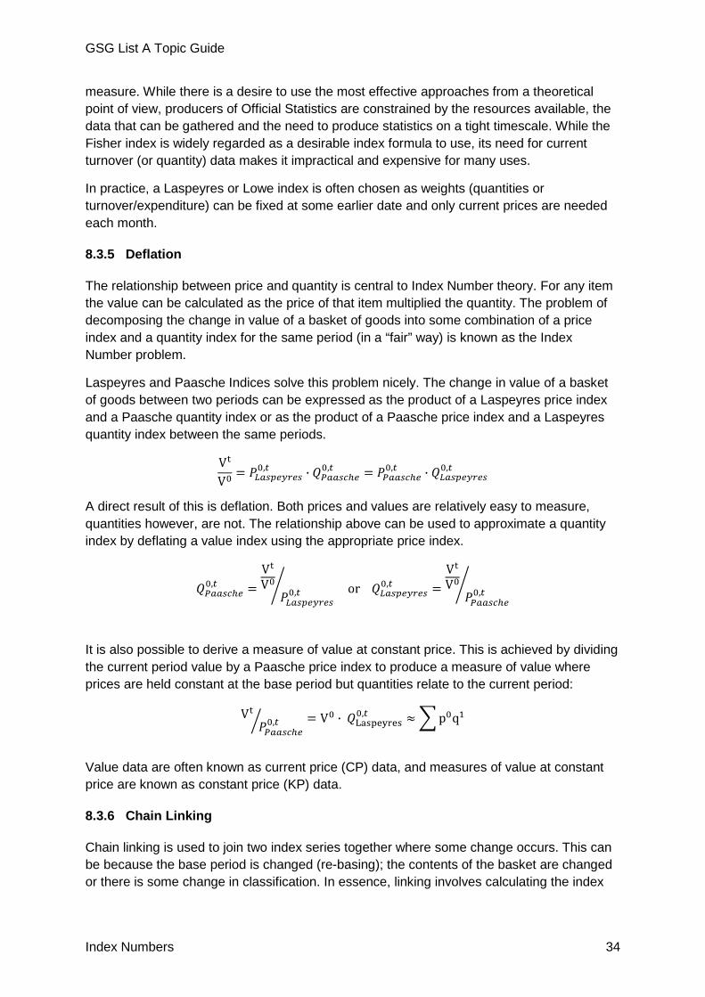
The relationship between price and quantity is central to Index Number theory. For any item the value can be calculated as the price of that item multiplied the quantity. The problem of decomposing the change in value of a basket of goods into some combination of a price index and a quantity index for the same period (in a “fair” way) is known as the Index Number problem.

Laspeyres and Paasche Indices solve this problem nicely. The change in value of a basket of goods between two periods can be expressed as the product of a Laspeyres price index and a Paasche quantity index or as the product of a Paasche price index and a Laspeyres quantity index between the same periods.

A direct result of this is deflation. Both prices and values are relatively easy to measure, quantities however, are not. The relationship above can be used to approximate a quantity index by deflating a value index using the appropriate price index.

It is also possible to derive a measure of value at constant price. This is achieved by dividing the current period value by a Paasche price index to produce a measure of value where prices are held constant at the base period but quantities relate to the current period:

Value data are often known as current price (CP) data, and measures of value at constant price are known as constant price (KP) data.

8.3.6 Chain Linking

Chain linking is used to join two index series together where some change occurs. This can be because the base period is changed (re-basing); the contents of the basket are changed or there is some change in classification. In essence, linking involves calculating the index


Index Numbers 35

under the old and new circumstances over some link period, and then applying the growth of the subsequent new series to the old series.

Chain-linking allows for the inclusion of new items in your basket of goods without either a break in the series or the recalculation of the entire index. Chain-linking can also be used to ensure that expenditure weights remain representative.


8.4.1 Assumptions

A number of assumptions are made when calculating index numbers. These can relate to the choice of index formula, the make-up of the basket of goods or services, or the choice of weights (both in terms of period and source) but all are determined by the target – what you are trying to measure, and any approach or framework that you choose to follow.

8.4.2 Consequences

There are many sources of bias in index numbers, mainly due to the fact that a large amount of information is being summarised into a single figure. It is important that data collected is representative of the population of interest and that weights and coverage are updated regularly to ensure that the index remains representative.

In practice weighted index formulae are preferred to un-weighted formulae; however weighting information (quantities or expenditure) can be difficult or expensive to collect at the individual item level. As a result, un-weighted indices are used at the lowest level of aggregation.


Index Numbers are used widely across government statistical outputs. The section below describes a few examples but does not constitute a full list of outputs. More recently, the uses of index numbers have extended far and wide. There are indices that provide measures of poverty, deprivation, freedom, prosperity and many other social and political topics.

8.5.1 Government Index Numbers

One of the most prominent outputs of the Office for National Statistics is the Consumer Price Index (CPI), which is a measure of the average change in the price of household goods and services. It is derived from a set of prices of goods and services from a (annually) fixed basket in a fixed geographic area. It is a temporal index (measured across time) with the base period (index value = 100) currently set to be 2005. The CPI is the preferred measure of UK inflation and it is published every month.

To achieve a representative measure of average price change, 180,000 prices are gathered every month on 650 individual goods and services in 150 randomly selected locations. The selection of goods and services is reviewed annually and the CPI combines all these individual prices to come up with one overall figure. The CPI is an annually chain linked Lowe Index which uses a combination of Jevons and Dütot Indices to combine prices at the


Index Numbers 36

Elementary Aggregate level. Other Indices produced by the ONS include GDP, the Retail Sales Index, the Index of Production, the Producer Price Index and the House Price Index.

Defence Analytical Services and Advice (DASA) within the Ministry of Defence, publishes defence inflation estimates. These measure the average change in pay and prices of goods and services, making up the defence budget, with quality and quantity held constant.

The estimate of defence inflation is a chain-linked Laspeyres price index. For each pair of consecutive years pure price growth is estimated by holding the quality and quantity of goods, services and personnel constant, and either directly measuring their change in price or making reference to relevant price indices. The year-on-year price growths are multiplied together to produce the chain-linked Laspeyres index with the reference period being the financial year 2004/05.

DEFRA uses indices for a number of key outputs. These include Total Factor productivity in agriculture, which is a chain-linked series of volumes weighted by values. The ‘basket’ by which it is measured covers a range of resources for agriculture with results measured in terms of the trend in volume of output leaving the industry per unit of all inputs (including labour).

8.5.2 Wider Applications

The well-known FTSE100 index is a measure of the change in the share price of the top 100 UK companies by market capitalisation. The base period is 3rd January 1984 with index value 1000. It is calculated every 15 seconds and is one of a family of stock related indices. It is a key indicator of investment conditions and appears in most news bulletins every day.

There are many examples of indices created to provide a view on other aspects of life, including the Multidimensional Poverty Index produced by the Department for International Development at the University of Oxford. This index has three dimensions: health, education, and standard of living. Although constrained by data limitations, it reveals a different pattern of poverty than pure income poverty.

8.6 Sources of Further Information

GSS Statistical Short Course: Index Numbers http://www.knowledgenetwork.gsi.gov.uk/statnet/statnet.nsf/15cc09bf3315edb180256b0700233105/d54edda9731dd35880257b2f00425df4/$FILE/GSS%20Statistical%20Training%20Unit%20ProspectusWEB.pdf

International Labour Organisation, Consumer Price Index Manual: Theory and Practice 2004 gauss.stat.su.se/master/es/CPIM-TP.pdf

UNECE Practical Guide to Producing the CPI www.unece.org/stats/publications/Practical_Guide_to_Producing_CPI.pdf

R G D Allen, Index Numbers in Economic Theory and Practice, Transaction Publishers, 1975

B M Balk, Price and Quantity Index Numbers, Cambridge University Press, 2008


Index Numbers 37


No specialist software is needed. Index Numbers can be calculated in spreadsheets or using statistical packages such as SAS and R.

government statistician group list a topics · 2014-02-07 · the gss statistician competence...

Documents