Google Vizier: A Service for Black-Box OptimizationDaniel Golovin

Google Research

dgg@google.com

Benjamin Solnik

Google Research

bsolnik@google.com

Subhodeep Moitra

Google Research

smoitra@google.com

Greg Kochanski

Google Research

gpk@google.com

John Karro

Google Research

karro@google.com

D. Sculley

Google Research

dsculley@google.com

ABSTRACT

Any sufficiently complex system acts as a black boxwhen it becomes

easier to experiment with than to understand. Hence, black-box

optimization has become increasingly important as systems have

become more complex. In this paper we describe Google Vizier, aGoogle-internal service for performing black-box optimization that

has become the de facto parameter tuning engine at Google. Google

Vizier is used to optimize many of our machine learning models

and other systems, and also provides core capabilities to Google’s

Cloud Machine Learning HyperTune subsystem. We discuss our

requirements, infrastructure design, underlying algorithms, and

advanced features such as transfer learning and automated early

stopping that the service provides.

KEYWORDS

Black-Box Optimization, Bayesian Optimization, Gaussian Pro-

cesses, Hyperparameters, Transfer Learning, Automated Stopping

1 INTRODUCTION

Black–box optimization is the task of optimizing an objective func-

tion f : X → Rwith a limited budget for evaluations. The adjective

“black–box” means that while we can evaluate f (x ) for any x ∈ X ,

we have no access to any other information about f , such as gradi-

ents or the Hessian. When function evaluations are expensive, it

makes sense to carefully and adaptively select values to evaluate;

the overall goal is for the system to generate a sequence of xt that

approaches the global optimum as rapidly as possible.

Black box optimization algorithms can be used to find the best

operating parameters for any system whose performance can be

measured as a function of adjustable parameters. It has many impor-

tant applications, such as automated tuning of the hyperparameters

of machine learning systems (e.g., learning rates, or the number

of hidden layers in a deep neural network), optimization of the

user interfaces of web services (e.g. optimizing colors and fonts

KDD ’17, August 13-17, 2017, Halifax, NS, Canada© 2017 Copyright held by the owner/author(s).

ACM ISBN 978-1-4503-4887-4/17/08.

https://doi.org/10.1145/3097983.3098043

to maximize reading speed), and optimization of physical systems

(e.g., optimizing airfoils in simulation).

In this paper we discuss a state-of-the-art system for black–box

optimization developed within Google, called Google Vizier, named

after a high official who offers advice to rulers. It is a service for

black-box optimization that supports several advanced algorithms.

The system has a convenient Remote Procedure Call (RPC) inter-

face, along with a dashboard and analysis tools. Google Vizier is

a research project, parts of which supply core capabilities to our

Cloud Machine Learning HyperTune1 subsystem. We discuss the ar-

chitecture of the system, design choices, and some of the algorithms

used.

1.1 Related Work

Black–box optimization makes minimal assumptions about the

problem under consideration, and thus is broadly applicable across

many domains and has been studied in multiple scholarly fields un-

der names including Bayesian Optimization [2, 25, 26], Derivative–

free optimization [7, 24], Sequential Experimental Design [5], and

assorted variants of the multiarmed bandit problem [13, 20, 29].

Several classes of algorithms have been proposed for the prob-

lem. The simplest of these are non-adaptive procedures such as

Random Search, which selects xt uniformly at random from X

at each time step t independent of the previous points selected,

xτ : 1 ≤ τ < t , and Grid Search, which selects along a grid (i.e.,

the Cartesian product of finite sets of feasible values for each pa-

rameter). Classic algorithms such as SimulatedAnnealing and

assorted genetic algorithms have also been investigated, e.g., Co-

variance Matrix Adaptation [16].

Another class of algorithms performs a local search by selecting

points thatmaintain a search pattern, such as a simplex in the case of

the classic Nelder–Mead algorithm [22]. More modern variants of

these algorithms maintain simple models of the objective f within

a subset of the feasible regions (called the trust region), and select a

point xt to improve the model within the trust region [7].

More recently, some researchers have combined powerful tech-

niques for modeling the objective f over the entire feasible region,

using ideas developed for multiarmed bandit problems for manag-

ing explore / exploit trade-offs. These approaches are fundamen-

tally Bayesian in nature, hence this literature goes under the name

Bayesian Optimization. Typically, the model for f is a Gaussian

1https://cloud.google.com/ml/

KDD 2017 Applied Data Science Paper KDD’17, August 13–17, 2017, Halifax, NS, Canada

1487

process (as in [26, 29]), a deep neural network (as in [27, 31]), or a

regression forest (as in [2, 19]).

Many of these algorithms have open-source implementations

available. Within the machine learning community, examples in-

clude, e.g., HyperOpt2, MOE

3, Spearmint

4, and AutoWeka

5, among

many others. In contrast to such software packages, which require

practitioners to set them up and run them locally, we opted to de-

velop a managed service for black–box optimization, which is more

convenient for users but involves additional design considerations.

1.2 Definitions

Throughout the paper, we use to the following terms to describe

the semantics of the system:

A Trial is a list of parameter values, x , that will lead to a single

evaluation of f (x ). A trial can be “Completed”, which means that it

has been evaluated and the objective value f (x ) has been assigned

to it, otherwise it is “Pending”.

A Study represents a single optimization run over a feasible

space. Each Study contains a configuration describing the feasible

space, as well as a set of Trials. It is assumed that f (x ) does not

change in the course of a Study.

AWorker refers to a process responsible for evaluating a PendingTrial and calculating its objective value.

2 SYSTEM OVERVIEW

This section explores the design considerations involved in imple-

menting black-box optimization as a service.

2.1 Design Goals and Constraints

Vizier’s design satisfies the following desiderata:

• Ease of use. Minimal user configuration and setup.

• Hosts state-of-the-art black-box optimization algorithms.

• High availability

• Scalable to millions of trials per study, thousands of parallel

trial evaluations per study, and billions of studies.

• Easy to experiment with new algorithms.

• Easy to change out algorithms deployed in production.

For ease of use, we implemented Vizier as a managed service

that stores the state of each optimization. This approach drastically

reduces the effort a new user needs to get up and running; and

a managed service with a well-documented and stable RPC API

allows us to upgrade the service without user effort. We provide a

default configuration for our managed service that is good enough

to ensure that most users need never concern themselves with the

underlying optimization algorithms.

The default option allows the service to dynamically select a

recommended black–box algorithm along with low–level settings

based on the study configuration.We choose tomake our algorithms

stateless, so that we can seamlessly switch algorithms during a

2https://github.com/jaberg/hyperopt

3https://github.com/Yelp/MOE

4https://github.com/HIPS/Spearmint

5https://github.com/automl/autoweka

study, dynamically choosing the algorithm that is likely to perform

better for a particular trial of a given study. For example, Gaussian

Process Bandits [26, 29] provide excellent result quality, but naive

implementations scale asO (n3) with the number of training points.

Thus, once we’ve collected a large number of completed Trials, we

may want to switch to using a more scalable algorithm.

At the same time, we want to allow ourselves (and advanced

users) the freedom to experiment with new algorithms or special-

case modifications of the supported algorithms in a manner that is

safe, easy, and fast. Hence, we’ve built Google Vizier as a modular

system consisting of four cooperating processes (see Figure 1) that

update the state of Studies in the central database. The processes

themselves are modular with several clean abstraction layers that

allow us to experiment with and apply different algorithms easily.

Finally wewant to allowmultiple trials to be evaluated in parallel,

and allow for the possibility that evaluating the objective function

for each trial could itself be a distributed process. To this end we

define Workers, responsible for evaluating suggestions, and iden-

tify each worker by a name (a worker_handle) that persists across

process preemptions or crashes.

2.2 Basic User Workflow

To use Vizier, a developer may use one of our client libraries (cur-

rently implemented in C++, Python, Golang), which will generate

service requests encoded as protocol buffers [15]. The basic work-

flow is extremely simple. Users specify a study configuration which

includes:

• Identifying characteristics of the study (e.g. name, owner,

permissions).

• The set of parameters along with feasible sets for each (c.f.,

Section 2.3.1 for details); Vizier does constrained optimiza-

tion over the feasible set.

Given this configuration, basic use of the service (with each trial

being evaluated by a single process) can be implemented as follows:

# Register this client with the Study, creating it if# necessary.client.LoadStudy(study_config, worker_handle)

while (not client.StudyIsDone()):

# Obtain a trial to evaluate.trial = client.GetSuggestion()

# Evaluate the objective function at the trial parameters.metrics = RunTrial(trial)

# Report back the results.client.CompleteTrial(trial, metrics)

Here RunTrial is the problem–specific evaluation of the objective

function f . Multiple named metrics may be reported back to Vizier,

however one must be distinguished as the objective value f (x ) for

trial x . Note that multiple processes working on a study should

share the same worker_handle if and only if they are collaboratively

evaluating the same trial. All processes registered with a given

study with the same worker_handle are guaranteed to receive the

same trial upon request, which enables distributed trial evaluation.

KDD 2017 Applied Data Science Paper KDD’17, August 13–17, 2017, Halifax, NS, Canada

1488

Vizier API

Persistent

Database

Suggestion Service

Suggestion

Workers

Automated Stopping Service

Dangling

Work Finder

AutomatedStopping

Workers

Evaluation

Workers

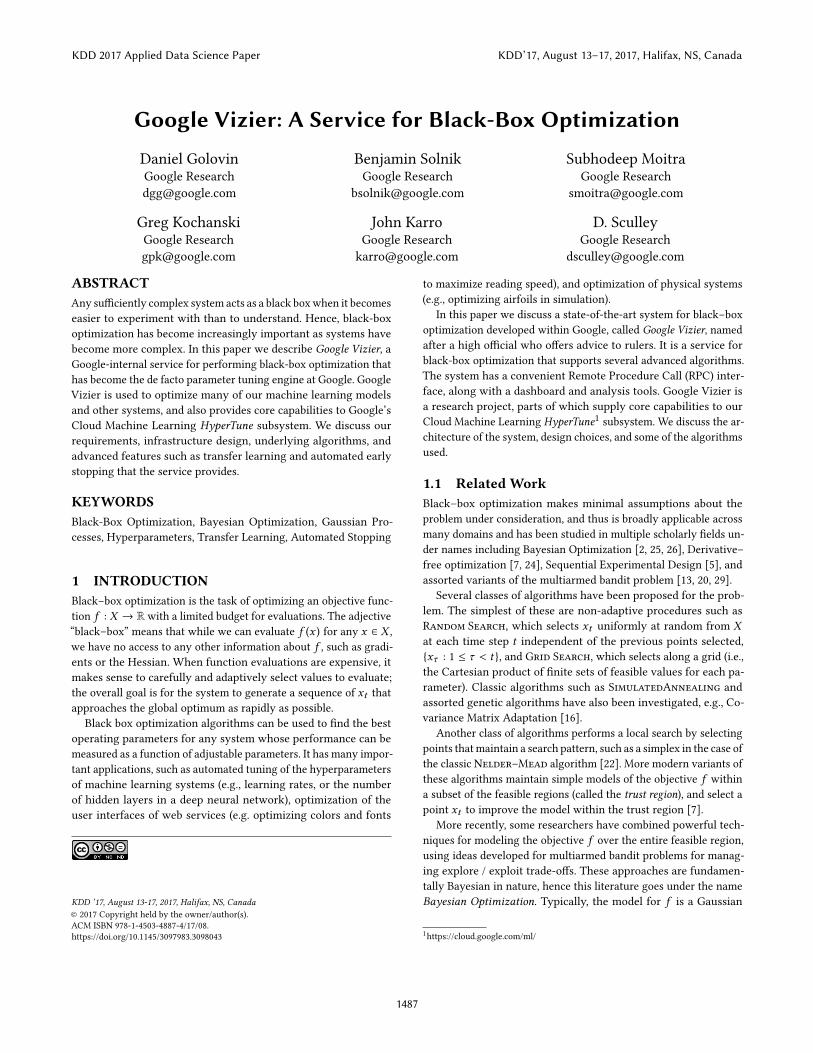
Figure 1: Architecture of Vizier service: Main components are (1)

Dangling work finder (restarts work lost to preemptions) (2) Persis-

tent Database holding the current state of all Studies (3) Suggestion

Service (creates new Trials), (4) Early Stopping Service (helps termi-

nate a Trial early) (5) Vizier API (JSON, validation, multiplexing) (6)

Evaluation workers (provided and owned by the user).

2.3 Interfaces

2.3.1 Configuring a Study. To configure a study, the user pro-vides a study name, owner, optional access permissions, an opti-

mization goal from MAXIMIZE, MINIMIZE, and specifies the feasible

region X via a set of ParameterConfigs, each of which declares a

parameter name along with its values. We support the following

parameter types:

• DOUBLE: The feasible region is a closed interval [a,b] for some

real values a ≤ b.

• INTEGER: The feasible region has the form [a,b]∩Z for some

integers a ≤ b.

• DISCRETE: The feasible region is an explicitly specified, or-

dered set of real numbers.

• CATEGORICAL: The feasible region is an explicitly specified,

unordered set of strings.

Users may also suggest recommended scaling, e.g., logarithmic

scaling for parameters for which the objective may depend only on

the order of magnitude of a parameter value.

2.3.2 API Definition. Workers and end users can make calls

to the Vizier Service using either a REST API or using Google’s

internal RPC protocol [15]. The most important service calls are:

• CreateStudy: Given a Study configuration, this creates an

optimization Study and returns a globally unique identifier

(“guid”) which is then used for all future service calls. If a

Study with a matching name exists, the guid for that Study

is returned. This allows parallel workers to call this method

and all register with the same Study.

• SuggestTrials: Thismethod takes a “worker handle” as input,

and immediately returns a globally unique handle for a “long-

running operation” that represents the work of generating

Trial suggestions. The user can then poll the API periodically

to check the status of the operation. Once the operation is

completed, it will contain the suggested Trials. This design

ensures that all service calls are made with low latency, while

allowing for the fact that the generation of Trials can take

longer.

• AddMeasurementToTrial: This method allows clients to pro-

vide intermediate metrics during the evaluation of a Trial.

These metrics are then used by the Automated Stopping

rules to determine which Trials should be stopped early.

• CompleteTrial: This method changes a Trial’s status to “Com-

pleted”, and provides a final objective value that is then used

to inform the suggestions provided by future calls to Sug-

gestTrials.

• ShouldTrialStop: This method returns a globally unique han-

dle for a long-running operation that represents the work of

determining whether a Pending Trial should be stopped.

2.4 Infrastructure

2.4.1 Parallel Processing of Suggestion Work. As the de factoparameter tuning engine of Google, Vizier is constantly working on

generating suggestions for a large number of Studies concurrently.

As such, a single machine would be insufficient for handling the

workload. Our Suggestion Service is therefore partitioned across

several Google datacenters, with a number of machines being used

in each one. Each instance of the Suggestion Service potentially

can generate suggestions for several Studies in parallel, giving

us a massively scalable suggestion infrastructure. Google’s load

balancing infrastructure is then used to allow clients to make calls

to a unified endpoint, without needing to know which instance is

doing the work.

When a request is received by a Suggestion Service instance to

generate suggestions, the instance first places a distributed lock on

the Study. This lock is acquired for a fixed period of time, and is

periodically extended by a separate thread running on the instance.

In other words, the lock will be held until either the instance fails,

or it decides it’s done working on the Study. If the instance fails

(due to e.g. hardware failure, job preemption, etc), the lock soon

expires, making it eligible to be picked up by a separate process

(called the “DanglingWorkFinder”) which then reassigns the Study

to a different Suggestion Service instance.

One consideration in maintaining a production system is that

bugs are inevitably introduced as our code matures. Occasionally, a

new algorithmic change, however well tested, will lead to instances

of the Suggestion Service failing for particular Studies. If a Study

is picked up by the DanglingWorkFinder too many times, it will

temporarily halt the Study and alert us. This prevents subtle bugs

that only affect a few Studies from causing crash loops that affect

the overall stability of the system.

2.5 The Algorithm Playground

Vizier’s algorithm playground provides a mechanism for advanced

users to easily, quickly, and safely replace Vizier’s core optimization

algorithms with arbitrary algorithms.

The playground serves a dual purpose; it allows rapid prototyp-

ing of new algorithms, and it allows power-users to easily customize

Vizier with advanced or exotic capabilities that are particular to

KDD 2017 Applied Data Science Paper KDD’17, August 13–17, 2017, Halifax, NS, Canada

1489

Vizier API

Persistent

Database

Evaluation

Workers

Playground Binary

Abstract PolicyCustom Policy

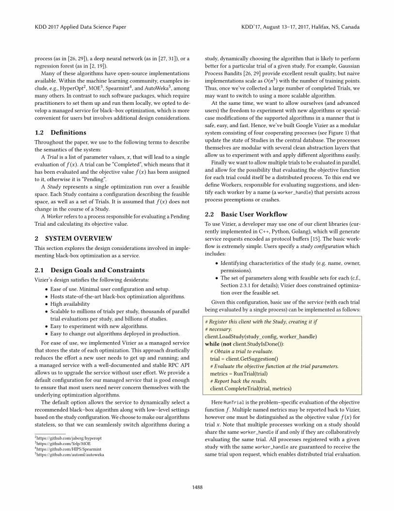
Figure 2: Architecture of Playground mode: Main components are

(1) The Vizier API takes service requests. (2) The Custom Policy im-

plements theAbstract Policy and generates suggested Trials. (3) The

Playground Binary drives the custom policy based on demand re-

ported by the Vizier API. (4) The EvaluationWorkers behave as nor-

mal, i.e., they request and evaluate Trials.

their use-case. In all cases, users of the playground benefit from

all of Vizier’s infrastructure aside from the core algorithms, such

as access to a persistent database of Trials, the dashboard, and

visualizations.

At the core of the playground is the ability to inject Trials into

a Study. Vizier allows the user or other authorized processes to

request one or more particular Trials be evaluated. In Playground

mode, Vizier does not suggest Trials for evaluation, but relies on

an external binary to generate Trials, which are then pushed to the

service for later distribution to the workers.

More specifically, the architecture of the Playground involves

the following key components: (1) Abstract Policy (2) PlaygroundBinary, (3) Vizier Service and (4) Evaluation Workers. See Figure 2for an illustration.

The Abstract Policy contains two abstract methods:

(1) GetNewSuggestions(trials, num_suggestions)

(2) GetEarlyStoppingTrials(trials)

which should be implemented by the user’s custom policy. Both

these methods are passed the full state of all Trials in the Study, so

algorithms may be implemented in a stateless fashion if desired.

GetNewSuggestions is expected to generate num_suggestions new tri-

als, while the GetEarlyStoppingTrialsmethod is expected to return

a list of Pending Trials that should be stopped early. The custom

policy is registered with the Playground Binary which periodically

polls the Vizier Service. The EvaluationWorkersmaintain the service

abstraction and are unaware of the existence of the Playground.

2.6 Benchmarking Suite

Vizier has an integrated framework that allows us to efficiently

benchmark our algorithms on a variety of objective functions. Many

of the objective functions come from the Black-Box Optimization

Benchmarking Workshop [10], but the framework allows for any

function to be modeled by implementing an abstract Experimenterclass, which has a virtual method responsible for calculating the

objective value for a given Trial, and a second virtual method that

returns the optimal solution for that benchmark.

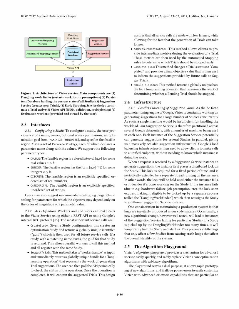
Figure 3: A section of the dashboard for tracking the progress of

Trials and the corresponding objective function values. Note also,

the presence of actions buttons such asGet Suggestions formanually

requesting suggestions.

Users configure a set of benchmark runs by providing a set of

algorithm configurations and a set of objective functions. The bench-

marking suite will optimize each function with each algorithm k

times (where k is configurable), producing a series of performance-

over-time metrics which are then formatted after execution. The

individual runs are distributed over multiple threads and multi-

ple machines, so it is easy to have thousands of benchmark runs

executed in parallel.

2.7 Dashboard and Visualizations

Vizier has a web dashboard which is used for both monitoring

and changing the state of Vizier studies. The dashboard is fully

featured and implements the full functionality of the Vizier API.

The dashboard is commonly used for: (1) Tracking the progress

of a study; (2) Interactive visualizations; (3) Creating, updating

and deleting a study; (4) Requesting new suggestions, early stop-

ping, activating/deactivating a study. See Figure 3 for a section of

the dashboard. In addition to monitoring and visualizations, the

dashboard contains action buttons such as Get Suggestions.The dashboard uses a translation layer which converts between

JSON and protocol buffers [15] when talking with backend servers.

The dashboard is built with Polymer [14] an open source web frame-

work supported by Google and uses material design principles. It

contains interactive visualizations for analyzing the parameters in

your study. In particular, we use the parallel coordinates visualiza-

tion [18] which has the benefit of scaling to high dimensional spaces

(∼15 dimensions) and works with both numerical and categorical

parameters. See Figure 4 for an example. Each vertical axis is a

dimension corresponding to a parameter, whereas each horizontal

line is an individual trial. The point at which the horizontal line

intersects the vertical axis gives the value of the parameter in that

dimension. This can be used for examining how the dimensions

co-vary with each other and also against the objective function

value (left most axis). The visualizations are built using d3.js [4].

KDD 2017 Applied Data Science Paper KDD’17, August 13–17, 2017, Halifax, NS, Canada

1490

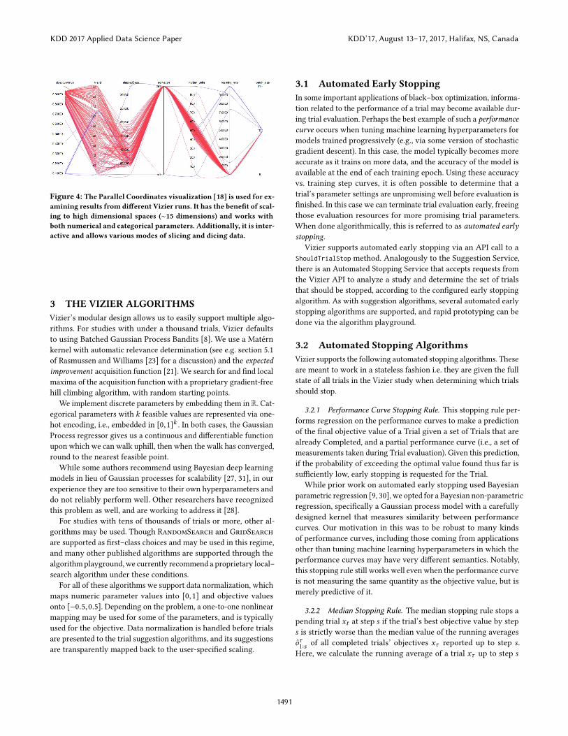
Figure 4: The Parallel Coordinates visualization [18] is used for ex-

amining results from different Vizier runs. It has the benefit of scal-

ing to high dimensional spaces (∼15 dimensions) and works with

both numerical and categorical parameters. Additionally, it is inter-

active and allows various modes of slicing and dicing data.

3 THE VIZIER ALGORITHMS

Vizier’s modular design allows us to easily support multiple algo-

rithms. For studies with under a thousand trials, Vizier defaults

to using Batched Gaussian Process Bandits [8]. We use a Matérn

kernel with automatic relevance determination (see e.g. section 5.1

of Rasmussen and Williams [23] for a discussion) and the expectedimprovement acquisition function [21]. We search for and find local

maxima of the acquisition function with a proprietary gradient-free

hill climbing algorithm, with random starting points.

We implement discrete parameters by embedding them in R. Cat-

egorical parameters with k feasible values are represented via one-

hot encoding, i.e., embedded in [0,1]k . In both cases, the Gaussian

Process regressor gives us a continuous and differentiable function

upon which we can walk uphill, then when the walk has converged,

round to the nearest feasible point.

While some authors recommend using Bayesian deep learning

models in lieu of Gaussian processes for scalability [27, 31], in our

experience they are too sensitive to their own hyperparameters and

do not reliably perform well. Other researchers have recognized

this problem as well, and are working to address it [28].

For studies with tens of thousands of trials or more, other al-

gorithms may be used. Though RandomSearch and GridSearch

are supported as first–class choices and may be used in this regime,

and many other published algorithms are supported through the

algorithm playground, we currently recommend a proprietary local–

search algorithm under these conditions.

For all of these algorithms we support data normalization, which

maps numeric parameter values into [0,1] and objective values

onto [−0.5,0.5]. Depending on the problem, a one-to-one nonlinear

mapping may be used for some of the parameters, and is typically

used for the objective. Data normalization is handled before trials

are presented to the trial suggestion algorithms, and its suggestions

are transparently mapped back to the user-specified scaling.

3.1 Automated Early Stopping

In some important applications of black–box optimization, informa-

tion related to the performance of a trial may become available dur-

ing trial evaluation. Perhaps the best example of such a performancecurve occurs when tuning machine learning hyperparameters for

models trained progressively (e.g., via some version of stochastic

gradient descent). In this case, the model typically becomes more

accurate as it trains on more data, and the accuracy of the model is

available at the end of each training epoch. Using these accuracy

vs. training step curves, it is often possible to determine that a

trial’s parameter settings are unpromising well before evaluation is

finished. In this case we can terminate trial evaluation early, freeing

those evaluation resources for more promising trial parameters.

When done algorithmically, this is referred to as automated earlystopping.

Vizier supports automated early stopping via an API call to a

ShouldTrialStop method. Analogously to the Suggestion Service,

there is an Automated Stopping Service that accepts requests from

the Vizier API to analyze a study and determine the set of trials

that should be stopped, according to the configured early stopping

algorithm. As with suggestion algorithms, several automated early

stopping algorithms are supported, and rapid prototyping can be

done via the algorithm playground.

3.2 Automated Stopping Algorithms

Vizier supports the following automated stopping algorithms. These

are meant to work in a stateless fashion i.e. they are given the full

state of all trials in the Vizier study when determining which trials

should stop.

3.2.1 Performance Curve Stopping Rule. This stopping rule per-

forms regression on the performance curves to make a prediction

of the final objective value of a Trial given a set of Trials that are

already Completed, and a partial performance curve (i.e., a set of

measurements taken during Trial evaluation). Given this prediction,

if the probability of exceeding the optimal value found thus far is

sufficiently low, early stopping is requested for the Trial.

While prior work on automated early stopping used Bayesian

parametric regression [9, 30], we opted for a Bayesian non-parametric

regression, specifically a Gaussian process model with a carefully

designed kernel that measures similarity between performance

curves. Our motivation in this was to be robust to many kinds

of performance curves, including those coming from applications

other than tuning machine learning hyperparameters in which the

performance curves may have very different semantics. Notably,

this stopping rule still works well even when the performance curve

is not measuring the same quantity as the objective value, but is

merely predictive of it.

3.2.2 Median Stopping Rule. The median stopping rule stops a

pending trial xt at step s if the trial’s best objective value by step

s is strictly worse than the median value of the running averages

oτ1:s of all completed trials’ objectives xτ reported up to step s .

Here, we calculate the running average of a trial xτ up to step s

KDD 2017 Applied Data Science Paper KDD’17, August 13–17, 2017, Halifax, NS, Canada

1491

as oτ1:s =

1

s Σsi=1o

τi , where o

τi is the objective value of xτ at step i .

As with the performance curve stopping rule, the median stopping

rule does not depend on a parametric model, and is applicable to a

wide range of performance curves. In fact, the median stopping rule

is model–free, and is more reminiscent of a bandit-based approach

such as HyperBand [20].

3.3 Transfer learning

When doing black-box optimization, users often run studies that are

similar to studies they have run before, and we can use this fact to

minimize repeatedwork. Vizier supports a form of Transfer Learningwhich leverages data from prior studies to guide and accelerate the

current study. For instance, one might tune the learning rate and

regularization of a machine learning system, then use that Study

as a prior to tune the same ML system on a different data set.

Vizier’s current approach to transfer learning is relatively simple,

yet robust to changes in objective across studies. We designed our

transfer learning approach with these goals in mind:

(1) Scale well to situations where there are many prior studies.

(2) Accelerate studies (i.e., achieve better results with fewer

trials) when the priors are good, particularly in cases where

the location of the optimum, x∗, doesn’t change much.

(3) Be robust against poorly chosen prior studies (i.e., a bad prior

should give only a modest deceleration).

(4) Share information even when there is no formal relationship

between the prior and current Studies.

In previous work on transfer learning in the context of hyper-

parameter optimization, Bardenet et al. [1] discuss the difficulty in

transferring knowledge across different datasets especially when

the observed metrics and the sampling of the datasets are different.

They use a ranking approach for constructing a surrogate model for

the response surface. This approach suffers from the computational

overhead of running a ranking algorithm. Yogatama and Mann [32]

propose a more efficient approach, which scales as Θ(kn + n3) for

k studies of n trials each, where the cubic term comes from using a

Gaussian process in their acquisition function.

Vizier typically uses Gaussian Process regressors, so one natural

approach to implementing transfer learning might be to build a

larger Gaussian Process regressor that is trained on both the prior(s)

and the current Study. However that approach fails to satisfy design

goal 1: for k studies with n trials each it would require Ω(k3n3)

time. Such an approach also requires one to specify or learn ker-

nel functions that bridge between the prior(s) and current Study,

violating design goal 4.

Instead, our strategy is to build a stack of Gaussian Process

regressors, where each regressor is associated with a study, and

where each level is trained on the residuals relative to the regressor

below it. Our model is that the studies were performed in a linear

sequence, each study using the studies before it as priors.

The bottom of the stack contains a regressor built using data

from the oldest study in the stack. The regressor above it is associ-

ated with the 2nd oldest study, and regresses on the residual of its

Figure 5: An illustration of our transfer learning scheme,

showing how µ ′i is built from the residual labels w.r.t. µi−1(shown in dotted red lines).

objective relative to the predictions of the regressor below it. Simi-

larly, the regressor associated with the ith study is built using the

data from that study, and regresses on the residual of the objective

with respect to the predictions of the regressor below it.

More formally, we have a sequence of studies Si ki=1 on un-

known objective functions

fiki=1, where the current study is Sk ,

and we build two sequences of regressors Ri ki=1 and

R′i

ki=1

hav-

ing posterior mean functions

µiki=1 and

µ ′i

ki=1

respectively, and

posterior standard deviation functions σi ki=1 and

σ ′i

ki=1

, respec-

tively. Our final predictions will be µk and σk .

Let Di =(x it ,y

it )tbe the dataset for study Si . Let R

′i be a re-

gressor trained using data

((x it ,y

it − µi−1 (x

it ))

twhich computes

µ ′i and σ ′i . Then we define as our posterior means at level i as

µi (x ) := µ ′i (x )+ µi−1 (x ). We take our posterior standard deviations

at level i , σi (x ), to be a weighted geometric mean of σ ′i (x ) and

σi−1 (x ), where the weights are a function of the amount of data

(i.e., completed trials) in Si and Si−1. The exact weighting function

depends on a constant α ≈ 1 sets the relative importance of old and

new standard deviations.

This approach has nice properties when the prior regressors

are densely supported (i.e. has many well-spaced data points), but

the top-level regressor has relatively little training data: (1) fine

structure in the priors carries through to µk , even if the top-level

regressor gives a low-resolution model of the objective function

residual; (2) since the estimate for σ ′k is inaccurate, averaging it

with σk−1 can lead to an improved estimate. Further, when the

top-level regressor has dense support, β → 1 and the σk → σ ′k , as

one might desire.

We provide details in the pseudocode in Algorithm 1, and illus-

trate the regressors in Figure 5.

Algorithm 1 is then used in the Batched Gaussian Process Ban-

dits [8] algorithm. Algorithm 1 has the property that for a suffi-

ciently dense sampling of the feasible region in the training data for

the current study, the predictions converge to those of a regressor

trained only on the current study data. This ensures a certain degree

of robustness: badly chosen priors will eventually be overwhelmed

(design goal 3).

KDD 2017 Applied Data Science Paper KDD’17, August 13–17, 2017, Halifax, NS, Canada

1492

Algorithm 1 Transfer Learning Regressor

# This is a higher order function that returns a regressor R(xtest);

# then R(xtest) can be evaluated to obtain (µ, σ )

function GetRegressor(Dtraining, i)

If i < 0: Return function that returns (0,1) for all inputs

# Recurse to get a Regressor (µi−1 (x ), σi−1 (x )) trained on

# the data for all levels of the stack below this one.

Rprior ← GetRegressor(Dtraining,i − 1)

# Compute training residuals

Dresiduals

← [(x ,y − Rprior (x )[0])for(x ,y) ∈ Di]

# Train a Gaussian Process (µ ′i (x ), σ′i (x )) on the residuals.

GPresiduals

= TrainGP(Dresiduals

)

function StackedRegressor(xtest)

µprior,σprior ← Rprior (xtest)

µtop,σtop ← GPresiduals

(xtest)

µ ← µtop + µpriorβ ← α |Di |/(α |Di | + |Di−1 |)

σ ← σβtop

σ1−βprior

return µ, σ

end function

return StackedRegressor

end function

In production settings, transfer learning is often particularly

valuable when the number of trials per study is relatively small,

but there are many such studies. For example, certain production

machine learning systems may be very expensive to train, limiting

the number of trials that can be run for hyperparameter tuning,

yet are mission critical for a business and are thus worked on year

after year. Over time, the total number of trials spanning several

small hyperparameter tuning runs can be quite informative. Our

transfer learning scheme is particularly well-suited to this case, as

illustrated in section 4.3.

4 RESULTS

4.1 Performance Evaluation

To evaluate the performance of Google Vizier we require functions

that can be used to benchmark the results. These are pre-selected,

easily calculated functions with known optimal points that have

proven challenging for black-box optimization algorithms. We can

measure the success of an optimizer on a benchmark function f by

its final optimality gap. That is, if x∗ minimizes f , and x is the best

solution found by the optimizer, then | f (x ) − f (x∗) | measures the

success of that optimizer on that function. If, as is frequently the

case, the optimizer has a stochastic component, we then calculate

the average optimality gap by averaging over multiple runs of the

optimizer on the same benchmark function.

Comparing between benchmarks is a more difficult given that the

different benchmark functions have different ranges and difficulties.

For example, a good black-box optimizer applied to the Rastrigin

function might achieve an optimality gap of 160, while simple

random sampling of the Beale function can quickly achieve an

optimality gap of 60 [10]. We normalize for this by taking the ratio

of the optimality gap to the optimality gap of Random Search on

the same function under the same conditions. Once normalized, we

average over the benchmarks to get a single value representing an

optimizer’s performance.

The benchmarks selected were primarily taken from the Black-

Box Optimization Benchmarking Workshop [10] (an academic com-

petition for black–box optimizers), and include the Beale, Branin,

Ellipsoidal, Rastrigin, Rosenbrock, Six Hump Camel, Sphere, and

Styblinski benchmark functions.

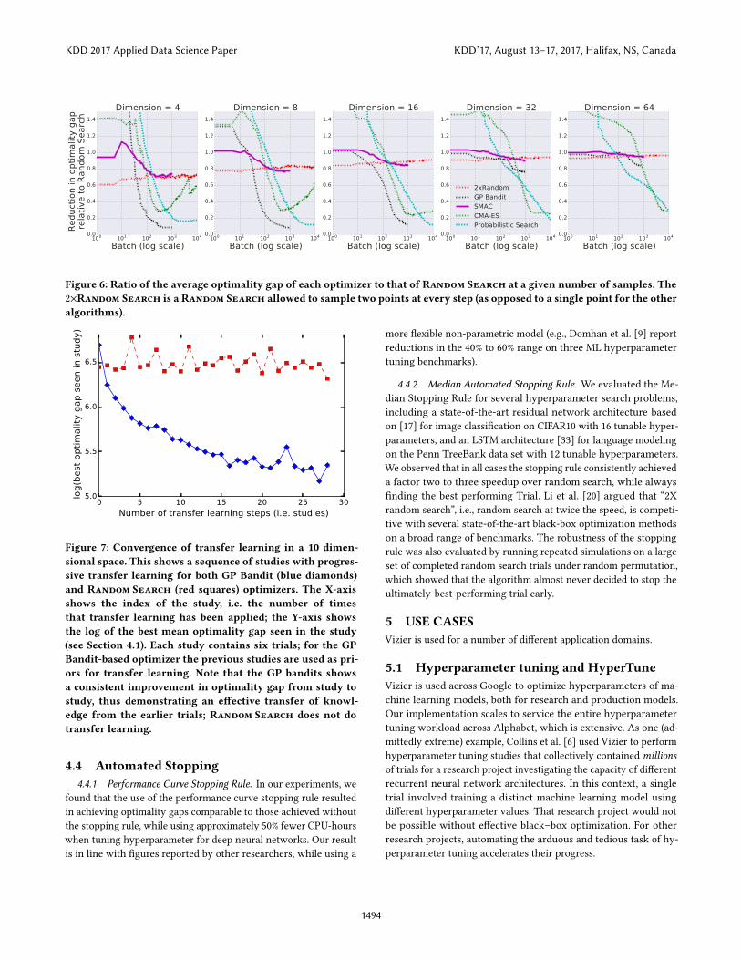
4.2 Empirical Results

In Figures 6 we look at result quality for four optimization algo-

rithms currently implemented in the Vizier framework: a multi-

armed bandit technique using a Gaussian process regressor [29],

the SMAC algorithm [19], the Covariance Matrix Adaption Evo-

lution Strategy (CMA-ES) [16], and a probabilistic search method

of our own. For a given dimension d , we generalized each bench-

mark function into a d dimensional space, ran each optimizer on

each benchmark 100 times, and recorded the intermediate results

(averaging these over the multiple runs). Figure 6 shows their im-

provement over Random Search; the horizontal axis represents

the number of trials have been evaluated, while the vertical axis

indicates each optimality gap as a fraction of the Random Search

optimality gap at the same point. The 2×Random Search curve is

the Random Search algorithm when it was allowed to sample two

points for each point the other algorithms evaluated. While some

authors have claimed that 2×Random Search is highly competitive

with Bayesian Optimization methods [20], our data suggests this

is only true when the dimensionality of the problem is sufficiently

high (e.g., over 16).

4.3 Transfer Learning

We display the value of transfer learning in Figure 7 with a series

of short studies; each study is just six trials long. Even so, one can

see that transfer learning from one study to the next leads to steady

progress towards the optimum, as the stack of regressors gradually

builds up information about the shape of the objective function.

This experiment is conducted in a 10 dimensional space, using

the 8 black-box functions described in section 4.1. We run 30 studies

(180 trials) and each study uses transfer learning from all previous

studies.

As one might hope, transfer learning causes the GP bandit algo-

rithm to show a strong systematic decrease in the optimality gap

from study to study, with its final average optimality gap 37% the

size of Random Search’s. As expected, Random Search shows no

systematic improvement in its optimality gap from study to study.

Note that a systematic improvement in the optimality gap is a

difficult task since each study gets a budget of only 6 trials whilst

operating in a 10 dimensional space, and the GP regressor is optimiz-

ing 8 internal hyperparameters for each study. By any reasonable

measure, a single study’s data is insufficient for the regressor to

learn much about the shape of the objective function.

KDD 2017 Applied Data Science Paper KDD’17, August 13–17, 2017, Halifax, NS, Canada

1493

100 101 102 103 104

Batch (log scale)

0.0

0.2

0.4

0.6

0.8

1.0

1.2

1.4

Reduct

ion in o

pti

malit

y g

ap

rela

tive t

o R

andom

Searc

h

Dimension = 4

100 101 102 103 104

Batch (log scale)

0.0

0.2

0.4

0.6

0.8

1.0

1.2

1.4

Dimension = 8

100 101 102 103 104

Batch (log scale)

0.0

0.2

0.4

0.6

0.8

1.0

1.2

1.4

Dimension = 16

100 101 102 103 104

Batch (log scale)

0.0

0.2

0.4

0.6

0.8

1.0

1.2

1.4

Dimension = 32

2xRandom

GP Bandit

SMAC

CMA-ES

Probabilistic Search

100 101 102 103 104

Batch (log scale)

0.0

0.2

0.4

0.6

0.8

1.0

1.2

1.4

Dimension = 64

Figure 6: Ratio of the average optimality gap of each optimizer to that of Random Search at a given number of samples. The

2×Random Search is a Random Search allowed to sample two points at every step (as opposed to a single point for the other

algorithms).

0 5 10 15 20 25 30

Number of transfer learning steps (i.e. studies)

5.0

5.5

6.0

6.5

log(b

est

opti

malit

y g

ap s

een in s

tudy)

Figure 7: Convergence of transfer learning in a 10 dimen-

sional space. This shows a sequence of studies with progres-

sive transfer learning for both GP Bandit (blue diamonds)

and Random Search (red squares) optimizers. The X-axis

shows the index of the study, i.e. the number of times

that transfer learning has been applied; the Y-axis shows

the log of the best mean optimality gap seen in the study

(see Section 4.1). Each study contains six trials; for the GP

Bandit-based optimizer the previous studies are used as pri-

ors for transfer learning. Note that the GP bandits shows

a consistent improvement in optimality gap from study to

study, thus demonstrating an effective transfer of knowl-

edge from the earlier trials; Random Search does not do

transfer learning.

4.4 Automated Stopping

4.4.1 Performance Curve Stopping Rule. In our experiments, we

found that the use of the performance curve stopping rule resulted

in achieving optimality gaps comparable to those achieved without

the stopping rule, while using approximately 50% fewer CPU-hours

when tuning hyperparameter for deep neural networks. Our result

is in line with figures reported by other researchers, while using a

more flexible non-parametric model (e.g., Domhan et al. [9] report

reductions in the 40% to 60% range on three ML hyperparameter

tuning benchmarks).

4.4.2 Median Automated Stopping Rule. We evaluated the Me-

dian Stopping Rule for several hyperparameter search problems,

including a state-of-the-art residual network architecture based

on [17] for image classification on CIFAR10 with 16 tunable hyper-

parameters, and an LSTM architecture [33] for language modeling

on the Penn TreeBank data set with 12 tunable hyperparameters.

We observed that in all cases the stopping rule consistently achieved

a factor two to three speedup over random search, while always

finding the best performing Trial. Li et al. [20] argued that “2X

random search”, i.e., random search at twice the speed, is competi-

tive with several state-of-the-art black-box optimization methods

on a broad range of benchmarks. The robustness of the stopping

rule was also evaluated by running repeated simulations on a large

set of completed random search trials under random permutation,

which showed that the algorithm almost never decided to stop the

ultimately-best-performing trial early.

5 USE CASES

Vizier is used for a number of different application domains.

5.1 Hyperparameter tuning and HyperTune

Vizier is used across Google to optimize hyperparameters of ma-

chine learning models, both for research and production models.

Our implementation scales to service the entire hyperparameter

tuning workload across Alphabet, which is extensive. As one (ad-

mittedly extreme) example, Collins et al. [6] used Vizier to perform

hyperparameter tuning studies that collectively contained millionsof trials for a research project investigating the capacity of different

recurrent neural network architectures. In this context, a single

trial involved training a distinct machine learning model using

different hyperparameter values. That research project would not

be possible without effective black–box optimization. For other

research projects, automating the arduous and tedious task of hy-

perparameter tuning accelerates their progress.

KDD 2017 Applied Data Science Paper KDD’17, August 13–17, 2017, Halifax, NS, Canada

1494

Perhaps even more importantly, Vizier has made notable im-

provements to production models underlying many Google prod-

ucts, resulting in measurably better user experiences for over a

billion people. External researchers and developers can achieve the

same benefits using Google Cloud Machine Learning HyperTunesubsystem, which benefits from our experience and technology.

5.2 Automated A/B testing

In addition to tuning hyperparameters, Vizier has a number of other

uses. It is used for automated A/B testing of Google web proper-

ties, for example tuning user–interface parameters such as font

and thumbnail sizes, color schema, and spacing, or traffic-serving

parameters such as the relative importance of various signals in

determining which items to show to a user. An example of the lat-

ter would be “how should the search results returned from Google

Maps trade off search-relevance for distance from the user?”

5.3 Delicious Chocolate Chip Cookies

Vizier is also used to solve complex black–box optimization prob-

lems arising from physical design or logistical problems. Here we

present an example that highlights some additional capabilities of

the system: finding the most delicious chocolate chip cookie recipe

from a parameterized space of recipes.

Parameters included baking soda, brown sugar, white

sugar, butter, vanilla, egg, flour, chocolate, chip type, salt, cayenne,

orange extract, baking time, and baking temperature. We provided

recipes to contractors responsible for providing desserts for Google

employees. The head chefs among the contractors were given dis-

cretion to alter parameters if (and only if) they strongly believed

it to be necessary, but would carefully note what alterations were

made. The cookies were baked, and distributed to the cafes for

taste–testing. Cafe goers tasted the cookies and provided feedback

via a survey. Survey results were aggregated and the results were

sent back to Vizier. The “machine learning cookies” were provided

about twice a week over several weeks.

The cookies improved significantly over time; later rounds were

extremely well-rated and, in the authors’ opinions, delicious. How-

ever, we wish to highlight the following capabilities of Vizier the

cookie design experiment exercised:

• Infeasible trials: In real applications, some trials may be in-feasible, meaning they cannot be evaluated for reasons that

are intrinsic to the parameter settings. Very high learning

rates may cause training to diverge, leading to garbage mod-

els. In this example: very low levels of butter may make your

cookie dough impossibly crumbly and incohesive.

• Manual overrides of suggested trials: Sometimes you cannot

evaluate the suggested trial or else mistakenly evaluate a

different trial than the one asked for. For example, when

baking you might be running low on an ingredient and have

to settle for less than the recommended amount.

• Transfer learning: Before starting to bake at large scale, we

baked some recipes in a smaller scale run-through. This pro-

vided useful data that we could transfer learn from when

baking at scale. Conditions were not identical, however, re-

sulting in some unexpected consequences. For example, the

dough was allowed to sit longer in large-scale production

which unexpectedly, and somewhat dramatically, increased

the subjective spiciness of the cookies for trials that involved

cayenne. Fortunately, our transfer learning scheme is rela-

tively robust to such shifts.

Vizier supports marking trials as infeasible, in which case they do

not receive an objective value. In the case of Bayesian Optimization,

previous work either assigns them a particularly bad objective

value, attempts to incorporate a probability of infeasibility into

the acquisition function to penalize points that are likely to be

infeasible [3], or tries to explicitly model the shape of the infeasible

region [11, 12]. We take the first approach, which is simple and

fairly effective for the applications we consider. Regarding manual

overrides, Vizier’s stateless designmakes it easy to support updating

or deleting trials; we simply update the trial state on the database.

For details on transfer learning, refer to section 3.3.

6 CONCLUSION

We have presented our design for Vizier, a scalable, state-of-the-

art internal service for black–box optimization within Google, ex-

plained many of its design choices, and described its use cases

and benefits. It has already proven to be a valuable platform for

research and development, and we expect it will only grow more so

as the area of black–box optimization grows in importance. Also,

it designs excellent cookies, which is a very rare capability among

computational systems.

7 ACKNOWLEDGMENTS

We gratefully acknowledge the contributions of the following:

Jeremy Kubica, Jeff Dean, Eric Christiansen, Moritz Hardt, Katya

Gonina, Kevin Jamieson, and Abdul Salem.

REFERENCES

[1] Rémi Bardenet, Mátyás Brendel, Balázs Kégl, and Michele Sebag. 2013. Collabo-

rative hyperparameter tuning. ICML 2 (2013), 199.

[2] James S Bergstra, Rémi Bardenet, Yoshua Bengio, and Balázs Kégl. 2011. Al-

gorithms for hyper-parameter optimization. In Advances in Neural InformationProcessing Systems. 2546–2554.

[3] J Bernardo, MJ Bayarri, JO Berger, AP Dawid, D Heckerman, AFM Smith, and

M West. 2011. Optimization under unknown constraints. Bayesian Statistics 9 9(2011), 229.

[4] Michael Bostock, Vadim Ogievetsky, and Jeffrey Heer. 2011. D3data-driven

documents. IEEE transactions on visualization and computer graphics 17, 12 (2011),2301–2309.

[5] Herman Chernoff. 1959. Sequential Design of Experiments. Ann. Math. Statist.30, 3 (09 1959), 755–770. https://doi.org/10.1214/aoms/1177706205

[6] Jasmine Collins, Jascha Sohl-Dickstein, and David Sussillo. 2017. Capacity and

Trainability in Recurrent Neural Networks. In Profeedings of the InternationalConference on Learning Representations (ICLR).

[7] Andrew R Conn, Katya Scheinberg, and Luis N Vicente. 2009. Introduction toderivative-free optimization. SIAM.

[8] Thomas Desautels, Andreas Krause, and Joel W Burdick. 2014. Parallelizing

exploration-exploitation tradeoffs in Gaussian process bandit optimization. Jour-nal of Machine Learning Research 15, 1 (2014), 3873–3923.

[9] Tobias Domhan, Jost Tobias Springenberg, and Frank Hutter. 2015. Speeding Up

Automatic Hyperparameter Optimization of Deep Neural Networks by Extrapo-

lation of Learning Curves.. In IJCAI. 3460–3468.

KDD 2017 Applied Data Science Paper KDD’17, August 13–17, 2017, Halifax, NS, Canada

1495

[10] Steffen Finck, Nikolaus Hansen, Raymond Rost, and Anne Auger. 2009.

Real-Parameter Black-Box Optimization Benchmarking 2009: Presentation of

the Noiseless Functions. http://coco.gforge.inria.fr/lib/exe/fetch.php?media=

download3.6:bbobdocfunctions.pdf. (2009). [Online].

[11] Jacob R Gardner, Matt J Kusner, Zhixiang Eddie Xu, Kilian Q Weinberger, and

John P Cunningham. 2014. Bayesian Optimization with Inequality Constraints..

In ICML. 937–945.[12] Michael A Gelbart, Jasper Snoek, and Ryan P Adams. 2014. Bayesian optimiza-

tion with unknown constraints. In Proceedings of the Thirtieth Conference onUncertainty in Artificial Intelligence. AUAI Press, 250–259.

[13] Josep Ginebra and Murray K. Clayton. 1995. Response Surface Bandits. Journalof the Royal Statistical Society. Series B (Methodological) 57, 4 (1995), 771–784.

http://www.jstor.org/stable/2345943

[14] Google. 2017. Polymer: Build modern apps using web components. https://github.

com/Polymer/polymer. (2017). [Online].

[15] Google. 2017. Protocol Buffers: Google’s data interchange format. https://github.

com/google/protobuf. (2017). [Online].

[16] Nikolaus Hansen and Andreas Ostermeier. 2001. Completely derandomized

self-adaptation in evolution strategies. Evolutionary computation 9, 2 (2001),

159–195.

[17] Kaiming He, Xiangyu Zhang, Shaoqing Ren, and Jian Sun. 2016. Deep residual

learning for image recognition. In Proceedings of the IEEE Conference on ComputerVision and Pattern Recognition. 770–778.

[18] Julian Heinrich and Daniel Weiskopf. 2013. State of the Art of Parallel Coordi-

nates.. In Eurographics (STARs). 95–116.[19] Frank Hutter, Holger H Hoos, and Kevin Leyton-Brown. 2011. Sequential model-

based optimization for general algorithm configuration. In International Confer-ence on Learning and Intelligent Optimization. Springer, 507–523.

[20] Lisha Li, Kevin G. Jamieson, Giulia DeSalvo, Afshin Rostamizadeh, and Ameet

Talwalkar. 2016. Hyperband: A Novel Bandit-Based Approach to Hyperparameter

Optimization. CoRR abs/1603.06560 (2016). http://arxiv.org/abs/1603.06560

[21] J Moćkus, V Tiesis, and A Źilinskas. 1978. The Application of Bayesian Methodsfor Seeking the Extremum. Vol. 2. Elsevier. 117–128 pages.

[22] John A Nelder and Roger Mead. 1965. A simplex method for function minimiza-

tion. The computer journal 7, 4 (1965), 308–313.[23] Carl Edward Rasmussen and Christopher K. I. Williams. 2005. Gaussian Processes

for Machine Learning (Adaptive Computation and Machine Learning). The MIT

Press.

[24] Luis Miguel Rios and Nikolaos V Sahinidis. 2013. Derivative-free optimization: a

review of algorithms and comparison of software implementations. Journal ofGlobal Optimization 56, 3 (2013), 1247–1293.

[25] Bobak Shahriari, Kevin Swersky, ZiyuWang, Ryan PAdams, and Nando de Freitas.

2016. Taking the human out of the loop: A review of bayesian optimization. Proc.IEEE 104, 1 (2016), 148–175.

[26] Jasper Snoek, Hugo Larochelle, and Ryan P Adams. 2012. Practical bayesian

optimization of machine learning algorithms. In Advances in neural informationprocessing systems. 2951–2959.

[27] Jasper Snoek, Oren Rippel, Kevin Swersky, Ryan Kiros, Nadathur Satish,

Narayanan Sundaram, Md. Mostofa Ali Patwary, Prabhat, and Ryan P. Adams.

2015. Scalable Bayesian Optimization Using Deep Neural Networks. In Pro-ceedings of the 32nd International Conference on Machine Learning, ICML 2015,Lille, France, 6-11 July 2015 (JMLR Workshop and Conference Proceedings), Fran-cis R. Bach and David M. Blei (Eds.), Vol. 37. JMLR.org, 2171–2180. http:

//jmlr.org/proceedings/papers/v37/snoek15.html

[28] Jost Tobias Springenberg, Aaron Klein, Stefan Falkner, and Frank Hut-

ter. 2016. Bayesian Optimization with Robust Bayesian Neural Net-

works. In Advances in Neural Information Processing Systems 29,D. D. Lee, M. Sugiyama, U. V. Luxburg, I. Guyon, and R. Garnett

(Eds.). Curran Associates, Inc., 4134–4142. http://papers.nips.cc/paper/

6117-bayesian-optimization-with-robust-bayesian-neural-networks.pdf

[29] Niranjan Srinivas, Andreas Krause, Sham Kakade, and Matthias Seeger. 2010.

Gaussian Process Optimization in the Bandit Setting: No Regret and Experimental

Design. ICML (2010).

[30] Kevin Swersky, Jasper Snoek, and Ryan Prescott Adams. 2014. Freeze-thaw

Bayesian optimization. arXiv preprint arXiv:1406.3896 (2014).[31] Andrew Gordon Wilson, Zhiting Hu, Ruslan Salakhutdinov, and Eric P Xing.

2016. Deep kernel learning. In Proceedings of the 19th International Conference onArtificial Intelligence and Statistics. 370–378.

[32] Dani Yogatama and Gideon Mann. 2014. Efficient Transfer Learning Method for

Automatic Hyperparameter Tuning. JMLR: W&CP 33 (2014), 1077–1085.

[33] Wojciech Zaremba, Ilya Sutskever, and Oriol Vinyals. 2014. Recurrent neural

network regularization. arXiv preprint arXiv:1409.2329 (2014).

KDD 2017 Applied Data Science Paper KDD’17, August 13–17, 2017, Halifax, NS, Canada

1496