good neighbor sip discussion october 24, 2014 gregory stella alpine geophysics, llc 1
TRANSCRIPT

1
Good Neighbor SIP Discussion
October 24, 2014
Gregory StellaAlpine Geophysics, LLC

2
History
• Discussions began in December of 2013 with the petition for the addition of Illinois, Indiana, Kentucky, Michigan, North Carolina, Ohio, Tennessee, Virginia, and West Virginia to the Ozone Transport Region (176A)
• Further conversations in May of 2014 where Tad introduced the Good Neighbor SIP process to help with MD’s ozone SIP due in June 2015
• Additional, regular conversations held regarding the modeling that has been conducted to support these two items

3
What Are We Trying To Resolve?
• MOG asked to conduct technical analyses to assist in the air quality assessment of an EGU optimization study– Run SCR/SNCR controls at optimized rates– Purpose to review controls to help MD reach
attainment

4
Current Air Quality Observations
• We’ve now seen most recent 2014 ozone concentration data showing Harford, MD in attainment of the 75 ppb NAAQS– Many other northeastern monitors also attain 8hr
ozone NAAQS
4th Highest MDA8 (ppm) 8hr Ozone DV (ppm)
State County Site ID 2009 2010 2011 2012 2013 2014* 2011-2013 2012-2014*
Maryland Harford 240251001 0.083 0.096 0.098 0.086 0.072 0.067 0.085 0.075
Maryland Harford 240259001 0.069 0.080 0.085 0.083 0.068 0.070 0.079 0.074
*Draft 4th high as of September 30, 2014
5
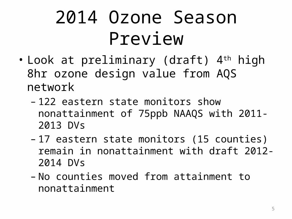
2014 Ozone Season Preview
• Look at preliminary (draft) 4th high 8hr ozone design value from AQS network– 122 eastern state monitors show nonattainment
of 75ppb NAAQS with 2011-2013 DVs– 17 eastern state monitors (15 counties) remain in
nonattainment with draft 2012-2014 DVs– No counties moved from attainment to
nonattainment

6
Nonattainment Monitors withDraft 2012/2014 8hr Ozone DVs
State Name County Name AQS Site ID2011-2013 Design
Value (ppm)2012-2014 Design
Value* (ppm)Connecticut Fairfield 090013007 0.089 0.082Michigan Allegan 260050003 0.086 0.082Connecticut Fairfield 090010017 0.083 0.079Indiana LaPorte 180910005 0.083 0.079Connecticut Fairfield 090019003 0.087 0.079Illinois Lake 170971007 0.080 0.079Michigan Berrien 260210014 0.082 0.078Ohio Lake 390850003 0.080 0.078Connecticut New Haven 090099002 0.089 0.078Connecticut Middlesex 090070007 0.081 0.078Michigan Muskegon 261210039 0.081 0.078Connecticut Tolland 090131001 0.077 0.078Maryland Cecil 240150003 0.082 0.078Connecticut New London 090110124 0.084 0.077Missouri Saint Charles 291831002 0.082 0.076Maryland Prince George's 240338003 0.081 0.076Illinois Cook 170310032 0.080 0.076
*Using draft 4th highest ozone concentrations as of September 30, 2014

7
176A Petition State MonitorsRecent 8hr Ozone Design Values
4th Highest MDA8 (ppb) 3yr Design Value (ppb)
Monitor County 2011 2012 2013 2014* 2011 2012 2013 2014*
240251001 Harford, Maryland 98 86 72 67 92 93 85 75
361030002 Suffolk, New York 89 83 72 61 84 85 87 72
90019003 Fairfield, Connecticut 87 89 86 61 79 85 87 79
421010024 Philadelphia, Pennsylvania 89 85 68 66 83 87 80 73
340150002 Gloucester, New Jersey 92 87 73 66 82 87 84 75
250070001 Dukes, Massachusetts 78 82 65 58 76 80 75 68
440090007 Washington, Rhode Island 74 82 79 60 73 78 78 74
100031007 New Castle, Delaware 78 82 62 71 75 80 74 72
330074001 Coos, New Hampshire 68 71 69 65 69 70 87 68
500030004 Bennington, Vermont 59 67 62 50 65 64 62 60
* As of 30 Sept 2014
8
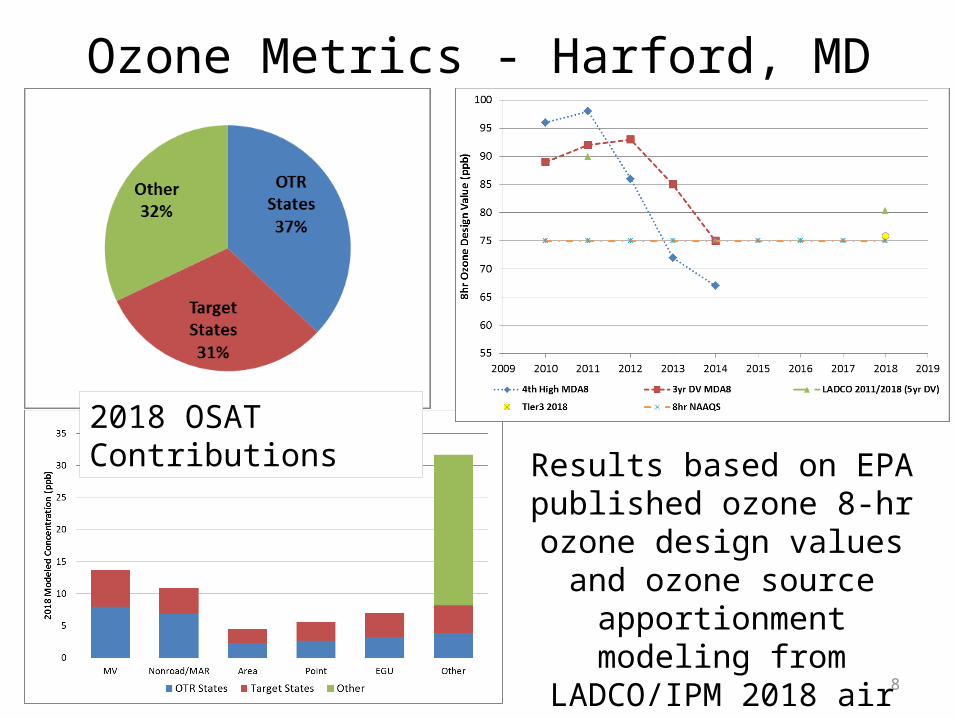
Ozone Metrics - Harford, MD
Results based on EPA published ozone 8-hr ozone design values
and ozone source apportionment modeling from
LADCO/IPM 2018 air quality simulations
2018 OSAT Contributions

9
Ozone Metrics – Suffolk, NY
Results based on EPA published ozone 8-hr ozone design values
and ozone source apportionment modeling from
LADCO/IPM 2018 air quality simulations
2018 OSAT Contributions

10
Ozone Metrics – Fairfield, CT
Results based on EPA published ozone 8-hr ozone design values
and ozone source apportionment modeling from
LADCO/IPM 2018 air quality simulations
2018 OSAT Contributions

11
Ozone Metrics – Philadelphia, PA
Results based on EPA published ozone 8-hr ozone design values
and ozone source apportionment modeling from
LADCO/IPM 2018 air quality simulations
2018 OSAT Contributions
12
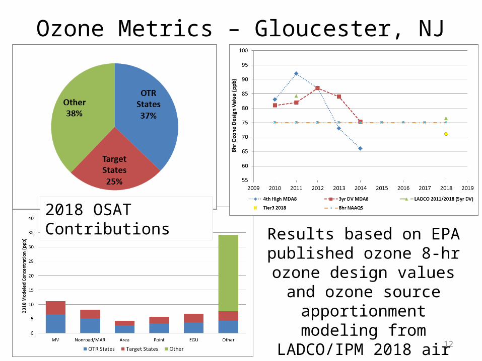
Ozone Metrics – Gloucester, NJ
Results based on EPA published ozone 8-hr ozone design values
and ozone source apportionment modeling from
LADCO/IPM 2018 air quality simulations
2018 OSAT Contributions

13
MD’s Good Neighbor Optimization
• MD picked 11 states– IL, IN, KY, MD, MI, NC, OH, PA, TN, VA, and WV– Optimized SCR/SNCR to lowest rate since 2005– MD predicts 0.9 ppb improvement in 2018 with
lowest rate optimization across all states

14
3rd Lowest Rate Optimization
• Developed list of SCR/SNCR units based on CEM data reporting
• Looked at 3rd lowest rate for optimization– Both SCR/SNCR results– Presumption that lowest rate occurs immediately
after installation– 3rd lowest rate allows for full year of operation
after installation and company optimization of controls

15
Emission / Air Quality Relationships
• Ratio development calculation relating 2011 ozone season summer episode (June through August) NOx emissions from EGU sources within each State to its ozone concentration air quality contribution at downwind monitors
• Designed to establish a NOx emissions to ozone concentration ratio that will be used in later stages of the analysis

16
Base Year Source-Receptor Analyses
• Base year (2011) APCA/OSAT to develop ozone source-receptor relationship data from CAMx simulation
17
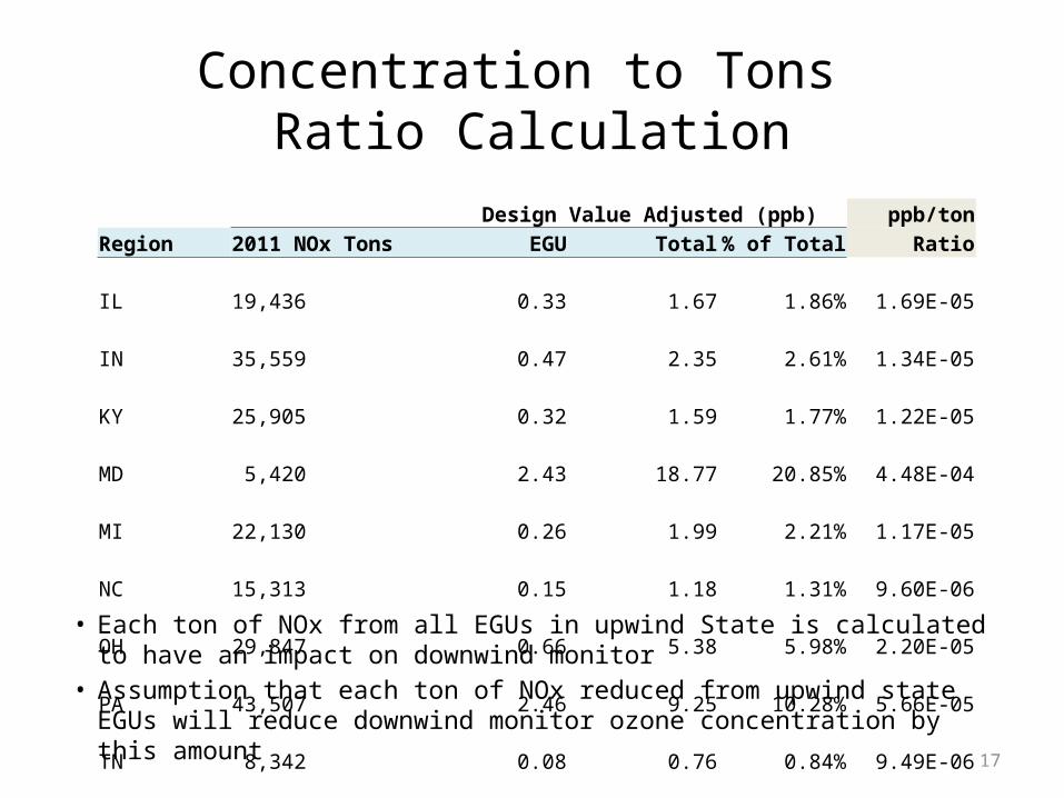
Concentration to Tons Ratio Calculation
• Each ton of NOx from all EGUs in upwind State is calculated to have an impact on downwind monitor
• Assumption that each ton of NOx reduced from upwind state EGUs will reduce downwind monitor ozone concentration by this amount
Design Value Adjusted (ppb) ppb/tonRegion 2011 NOx Tons EGU Total % of Total RatioIL 19,436 0.33 1.67 1.86% 1.69E-05IN 35,559 0.47 2.35 2.61% 1.34E-05KY 25,905 0.32 1.59 1.77% 1.22E-05MD 5,420 2.43 18.77 20.85% 4.48E-04MI 22,130 0.26 1.99 2.21% 1.17E-05NC 15,313 0.15 1.18 1.31% 9.60E-06OH 29,847 0.66 5.38 5.98% 2.20E-05PA 43,507 2.46 9.25 10.28% 5.66E-05TN 8,342 0.08 0.76 0.84% 9.49E-06VA/DC 11,014 0.69 6.38 7.08% 6.26E-05WV 16,496 0.84 2.49 2.76% 5.07E-05Grand Total 10.23 90.00 100.00%

18
Emission Inventory Assessment
• Match 2011 modeling platform of EGU emissions to CAMD reported metadata and identify which units have post-combustion NOx control (SCR / SNCR) installed for operation
• Using other historical CAMD data (ozone season 2005-2013 emission and operating reports), we made a preliminary determination as to which units in 2011 were operating these post-combustion controls during the summer episode

19
SCR/SNCR - Top Reducing Units2011 Ozone Season
NOx Rate NOxNOx Rate
(lbs/MMBtu) NOx Reduction (Tons)
State Facility ORIS UNIT(lbs/
MMBtu) (Tons) Lowest3rd
Lowest Lowest 3rd LowestPA Keystone 3136 2 0.364 5,044.3 0.043 0.045 -4,444.3 -4,415.2PA Keystone 3136 1 0.374 4,854.6 0.043 0.052 -4,294.7 -4,177.8PA Montour 3149 1 0.331 3,298.4 0.058 0.084 -2,720.1 -2,465.3OH W H Zimmer 6019 1 0.217 3,559.5 0.056 0.075 -2,638.4 -2,338.4PA Montour 3149 2 0.316 3,132.2 0.058 0.094 -2,559.4 -2,203.7KY Paradise 1378 3 0.332 2,431.2 0.100 0.108 -1,698.0 -1,640.2IN Gibson 6113 2 0.226 2,043.4 0.067 0.098 -1,437.0 -1,163.5WV Harrison Power Station 3944 3 0.214 1,834.2 0.066 0.072 -1,269.7 -1,213.9IN Gibson 6113 1 0.182 1,504.5 0.034 0.071 -1,221.1 -917.1WV Harrison Power Station 3944 2 0.201 1,774.7 0.066 0.080 -1,190.9 -1,072.7WV Harrison Power Station 3944 1 0.191 1,698.4 0.063 0.079 -1,134.2 -997.2IL Kincaid Station 876 2 0.204 1,566.7 0.060 0.062 -1,104.9 -1,086.4PA Hatfield's Ferry Station 3179 3 0.439 2,848.0 0.270 0.368 -1,098.9 -466.4PA Cheswick 8226 1 0.235 1,690.0 0.090 0.171 -1,043.4 -462.8

20
Emission/Air Quality Change Calculation
• Calculate the State-level difference in EGU NOx emissions resulting from the application of post-combustion NOx control compared to actual 2011 operations– in cases where post-combustion control was already in
operation at lowest rates or units are not identified to have SNCR/SCR installed, this value will be zero
• Apply this value to each State-monitor where we have generated an emissions to air quality change ratio
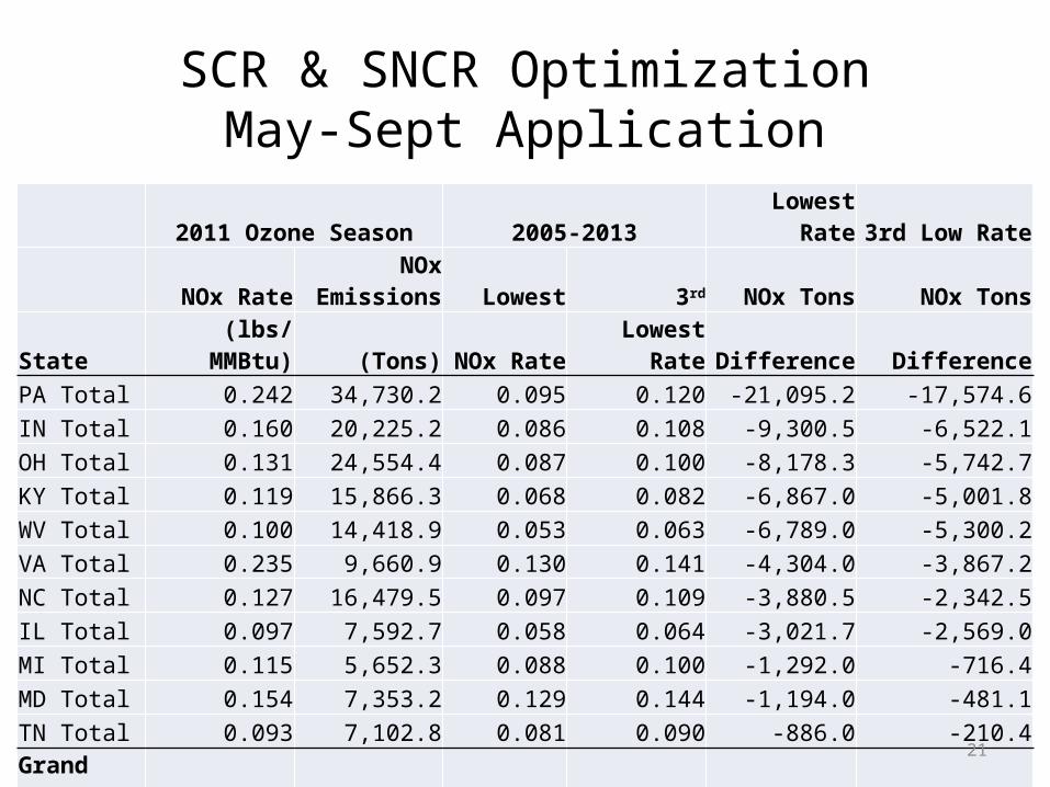
21
SCR & SNCR OptimizationMay-Sept Application
2011 Ozone Season 2005-2013 Lowest Rate 3rd Low RateNOx Rate NOx Emissions Lowest 3rd NOx Tons NOx Tons
State (lbs/MMBtu) (Tons) NOx Rate Lowest Rate Difference DifferencePA Total 0.242 34,730.2 0.095 0.120 -21,095.2 -17,574.6IN Total 0.160 20,225.2 0.086 0.108 -9,300.5 -6,522.1OH Total 0.131 24,554.4 0.087 0.100 -8,178.3 -5,742.7KY Total 0.119 15,866.3 0.068 0.082 -6,867.0 -5,001.8WV Total 0.100 14,418.9 0.053 0.063 -6,789.0 -5,300.2VA Total 0.235 9,660.9 0.130 0.141 -4,304.0 -3,867.2NC Total 0.127 16,479.5 0.097 0.109 -3,880.5 -2,342.5IL Total 0.097 7,592.7 0.058 0.064 -3,021.7 -2,569.0MI Total 0.115 5,652.3 0.088 0.100 -1,292.0 -716.4MD Total 0.154 7,353.2 0.129 0.144 -1,194.0 -481.1TN Total 0.093 7,102.8 0.081 0.090 -886.0 -210.4Grand Total 0.141 163,636.3 0.084 0.098 -66,808.1 -50,328.1

22
Optimization Application
• Calculation at each monitor was conducted for each upwind State with ozone contribution (significant or not)

23
June-August Optimization NOxAll EGU Emissions

24
June – August Optimization OzoneHarford, MD Monitor
Lowest Rate Strategy (ppb) 3rd Lowest Rate Strategy (ppb)
RegionTons Red EGU Delta Total
% of Total
Tons Red EGU Delta Total
% of Total
IL -1,808 0.30 0.03 1.64 1.86% -1,522 0.30 0.03 1.65 1.86%
IN -5,704 0.40 0.08 2.28 2.58% -4,007 0.42 0.05 2.30 2.59%
KY -4,687 0.26 0.06 1.54 1.74% -3,547 0.27 0.04 1.55 1.75%
MD -723 2.11 0.32 18.44 20.90% -249 2.32 0.11 18.65 21.03%
MI -797 0.25 0.01 1.98 2.24% -467 0.25 0.01 1.98 2.24%
NC -2,349 0.12 0.02 1.15 1.31% -1,554 0.13 0.01 1.16 1.31%
OH -5,254 0.56 0.10 5.28 5.98% -3,645 0.58 0.08 5.30 5.98%
PA -13,360 1.71 0.76 8.49 9.62% -11,107 1.84 0.63 8.62 9.71%
TN -538 0.07 0.01 0.75 0.85% -133 0.08 0.00 0.76 0.85%
VA/DC -2,404 0.54 0.15 6.23 7.06% -2,143 0.56 0.13 6.24 7.04%
WV -4,543 0.61 0.23 2.26 2.56% -3,587 0.65 0.18 2.31 2.60%
Grand Total -42,166 8.47 1.76 88.24 100.00% -31,962 8.95 1.28 88.72 100.00%

25
Air Quality Effectiveness Calculation
• Apply emission change to each State-monitor and generate an emissions to air quality change ratio
• From optimization results, developed EGU reduction effectiveness factor from 2011 modeling and OSAT results– Looks at effectiveness of ton reduced on downwind
ozone concentration change– Calculated for each monitor

26
OSAT/ Reduction Efficiency (SCR/SNCR)Jun-Aug 2011 Optimization
Harford, MD Monitor
Compare total 2011 reduction of 1.28 ppb with MD estimate of 0.9 ppb in 2018.MD/PA comprise 58% (0.74 ppb) of ozone reduction under 3rd lowest rate strategy.
EfficiencyNOx Tons Change in Factor
State Reduced O3 (ppb) ppb/ton redPA 11,107 0.63 5.66E-05WV 3,587 0.18 5.07E-05VA/DC 2,143 0.13 6.26E-05MD 249 0.11 4.48E-04OH 3,645 0.08 2.20E-05IN 4,007 0.05 1.34E-05KY 3,547 0.04 1.22E-05IL 1,522 0.03 1.69E-05NC 1,554 0.01 9.60E-06MI 467 0.01 1.17E-05TN 133 0.00 9.49E-06Total 31,962 1.28

27
Efficiency Comparison• Optimization of EGU controls in MD has almost an order of
magnitude greater impact on Harford monitor than any other state
MD VA/DC PA WV OH IL IN KY MI NC TN0.000
0.100
0.200
0.300
0.400
0.500
Ozone ppb Decrease with 1,000 Ton EGU Reduction
Ozo
ne R
educ
tion
(ppb
)

28
2018 Attainment Results
• Ran EPA attainment model (MATS) on LADCO 2018 modeling platform– Based on EPA EGU modeling with IPM– Includes results of onroad Tier3 NPRM– Compare to final Tier3 EPA dv modeling, MD
scenario application, current draft 3yr dvs

29
2018 Ozone DVsEastern US Modeling Domain
LADCO Modeling DV (ppb) Tier3 MD 3C 2012-14Location 2011 DV 2018 DV 2018 DV 2018 DV 3yr DVHarford, Maryland 90.0 80.4 75.87 74.7 75Suffolk, New York 83.3 78.7 78.52Fairfield, Connecticut 83.7 77.8 75.16New Haven, Connecticut 85.7 77.8 72.28Sheboygan, Wisconsin 84.3 77.0 71.57Philadelphia, Pennsylvania 83.3 76.6 77.32Gloucester, New Jersey 84.3 76.5 71.13Hamilton, Ohio 82.0 76.2 71.57Jefferson, Kentucky 82.0 76.0 69.25Wayne, Michigan 78.7 75.8 74.13Saint Charles, Missouri 82.3 75.6 72.56Allegan, Michigan 82.7 75.5 74.44Allegheny, Pennsylvania 80.7 74.9 72.91Franklin, Ohio 80.3 74.7 70.71Oldham, Kentucky 82.0 74.6 66.48Arlington, Virginia 81.7 74.0 69.43Fairfax, Virginia 82.3 74.0 69.25Cecil, Maryland 83.0 73.8 72.82
MD 2018 results lower than LADCO or Tier3Why?

30
MD’s Path to Attainment

31
“The Bottom Line”Case / Strategy Reduction Ozone dvMD 2018 DV 79 ppb
Tier 3 ~ 0.8 ppb 78.2Add'l OTR Measures ~ 1.2 77.0
Add’l MD Only Controls ~ 1.4 75.6 <- Already Attainment
EGU Optimized (MD/PA) ~ 0.5 75.1 58% of Total Optimization
Attainment achieved without Upwind State ControlsEGU Optimized (Upwind) ~ 0.4 74.7
MD 2018 Scenarios DV 74.7WOE ~ 0.5
MOVES2014/MEGAN Lower (?)PA NOx RACT Lower
Unit Retirements Lower

32
Conclusions
• Current Harford monitoring data points to attainment of 75 ppb NAAQS
• 2018 modeling data projects Harford attainment without additional upwind controls
• Is there other justification for upwind control?