GNSS Signal Tracking Using a Bank of

Correlators

Karen Q.Z. Chiang, Cornell University

Mark L. Psiaki, Cornell University

BIOGRAPHIES

Karen Q.Z. Chiang received a B.S. in Applied Physics

from Columbia University in 2009. She is currently a

second-year Ph.D. student in the Sibley School of

Mechanical and Aerospace Engineering at Cornell

University. Her area of interest is GNSS applications for

model-based estimation.

Mark L. Psiaki is a Professor in the Sibley School of

Mechanical and Aerospace Engineering. He received a

B.A. in Physics and M.A. and Ph.D. degrees in

Mechanical and Aerospace Engineering from Princeton

University. His research interests are in the areas of

estimation and filtering, spacecraft attitude and orbit

determination, and GNSS technology and applications.

ABSTRACT

A combined PLL/DLL algorithm is developed for

tracking GNSS carrier phase and code phase using the

output from a large number of correlators. This approach

has advantages for limb-scanning applications, in which

useful meteorological information, available only at the

initial rising time of a GPS satellite, is desired. The

technique uses the bank of correlators to span wide ranges

of uncertainty in code phase and carrier phase, thereby

avoiding the need for a separate acquisition and the

associated loss of an initial span of data. A fusion of

optimal estimation methods processes the output from

these correlators. A batch optimization of a signal

model’s fit to the many accumulations provides the

Kalman filter with “measurements” of the most likely

signal parameters, and the Kalman filter utilizes a signal

dynamics model to provide estimates that drive the PLL

and DLL.

The effectiveness of this algorithm is demonstrated by

using a truth-model simulation of a limb scan. With this

method and 50 Hz accumulations, pull-ins of at minimum

122 Hz and 5 C/A code chips, for the PLL and DLL

respectively, are achieved. Moreover, uncertainties and

errors for all signal parameters are rapidly driven close to

zero. The rising signal is tracked successfully from

approximately 0.03 s since emergence.

I. INTRODUCTION

GNSS receivers must achieve and maintain lock on

carrier Doppler shift and the pseudo-random number

(PRN) code phase in order to properly track a signal and

ascertain navigation observables. A standard GNSS

receiver accomplishes this with two separate, consecutive

operations: acquisition and tracking 1. Acquisition

searches for initial estimates of Doppler shift and PRN

code phase. The tracking algorithm then uses these

estimates to initiate a delay-locked loop (DLL), and either

a frequency-locked loop (FLL) or a phase-locked loop

(PLL), to respectively keep the replicas of the code and

carrier signal aligned with those of the received signal.

The objective of this paper is to create a joint PLL/DLL

algorithm that functions normally even with large

tracking errors, and that does not require the usual

transition from initial acquisition to tracking. The

primary motivation for such an algorithm is to equip a

LEO satellite, acting as a GPS receiver, with the means to

capture data from a rising-GPS-satellite limb scan,

without any loss of data during the time it would take to

carry out a standard acquisition.

To realize this goal of robustness and speed, the new

tracking algorithm utilizes a bank of correlators to

encompass uncertainties in code phase and Doppler shift,

forming rectangular regions within Doppler-shift/code-

phase space. Figure 1 illustrates this concept. Note that

indicates the Doppler shift axis, and indicates the

PRN code delay axis.

In the space of these two signal properties, with time as a

parameter, the estimated trajectory begins at the first

estimate of Doppler shift and code phase. The uncertainty

at this time is relatively large, but the bank of correlators

spans a range that contains the true point. As time

progresses, the level of uncertainty may change. In the

case depicted, the level shrinks, and therefore the size of

correlator bank will also decrease.

Copyright © 2010 by Karen Q.Z. Chiang and Mark L. Psiaki. All rights reserved. Preprint from ION GNSS 2010

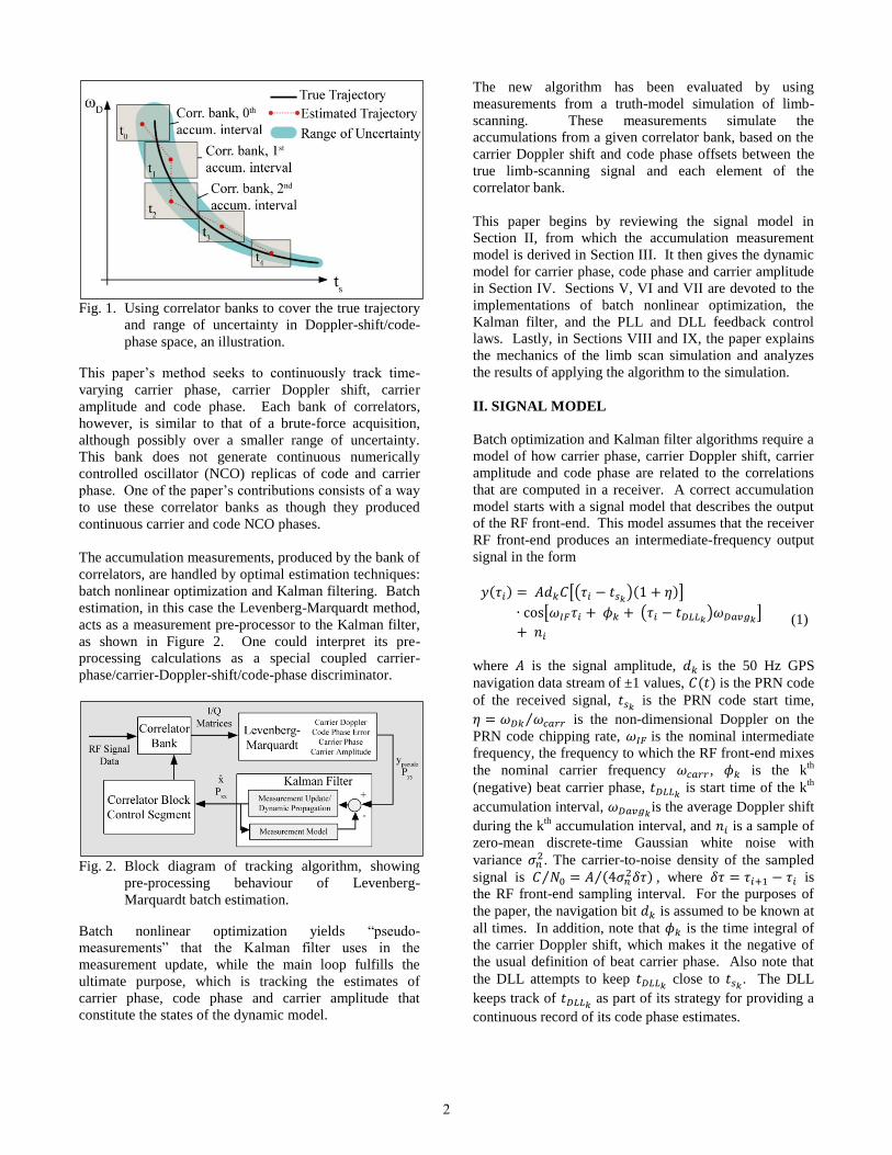
Fig. 1. Using correlator banks to cover the true trajectory

and range of uncertainty in Doppler-shift/code-

phase space, an illustration.

This paper’s method seeks to continuously track time-

varying carrier phase, carrier Doppler shift, carrier

amplitude and code phase. Each bank of correlators,

however, is similar to that of a brute-force acquisition,

although possibly over a smaller range of uncertainty.

This bank does not generate continuous numerically

controlled oscillator (NCO) replicas of code and carrier

phase. One of the paper’s contributions consists of a way

to use these correlator banks as though they produced

continuous carrier and code NCO phases.

The accumulation measurements, produced by the bank of

correlators, are handled by optimal estimation techniques:

batch nonlinear optimization and Kalman filtering. Batch

estimation, in this case the Levenberg-Marquardt method,

acts as a measurement pre-processor to the Kalman filter,

as shown in Figure 2. One could interpret its pre-

processing calculations as a special coupled carrier-

phase/carrier-Doppler-shift/code-phase discriminator.

Fig. 2. Block diagram of tracking algorithm, showing

pre-processing behaviour of Levenberg-

Marquardt batch estimation.

Batch nonlinear optimization yields “pseudo-

measurements” that the Kalman filter uses in the

measurement update, while the main loop fulfills the

ultimate purpose, which is tracking the estimates of

carrier phase, code phase and carrier amplitude that

constitute the states of the dynamic model.

The new algorithm has been evaluated by using

measurements from a truth-model simulation of limb-

scanning. These measurements simulate the

accumulations from a given correlator bank, based on the

carrier Doppler shift and code phase offsets between the

true limb-scanning signal and each element of the

correlator bank.

This paper begins by reviewing the signal model in

Section II, from which the accumulation measurement

model is derived in Section III. It then gives the dynamic

model for carrier phase, code phase and carrier amplitude

in Section IV. Sections V, VI and VII are devoted to the

implementations of batch nonlinear optimization, the

Kalman filter, and the PLL and DLL feedback control

laws. Lastly, in Sections VIII and IX, the paper explains

the mechanics of the limb scan simulation and analyzes

the results of applying the algorithm to the simulation.

II. SIGNAL MODEL

Batch optimization and Kalman filter algorithms require a

model of how carrier phase, carrier Doppler shift, carrier

amplitude and code phase are related to the correlations

that are computed in a receiver. A correct accumulation

model starts with a signal model that describes the output

of the RF front-end. This model assumes that the receiver

RF front-end produces an intermediate-frequency output

signal in the form

( ) [( )( )]

[ ( )

]

(1)

where is the signal amplitude, is the 50 Hz GPS

navigation data stream of ±1 values, ( ) is the PRN code

of the received signal, is the PRN code start time,

⁄ is the non-dimensional Doppler on the

PRN code chipping rate, is the nominal intermediate

frequency, the frequency to which the RF front-end mixes

the nominal carrier frequency , is the kth

(negative) beat carrier phase, is start time of the k

th

accumulation interval, is the average Doppler shift

during the kth

accumulation interval, and is a sample of

zero-mean discrete-time Gaussian white noise with

variance . The carrier-to-noise density of the sampled

signal is ⁄ ( )⁄ , where is

the RF front-end sampling interval. For the purposes of

the paper, the navigation bit is assumed to be known at

all times. In addition, note that is the time integral of

the carrier Doppler shift, which makes it the negative of

the usual definition of beat carrier phase. Also note that

the DLL attempts to keep close to

. The DLL

keeps track of as part of its strategy for providing a

continuous record of its code phase estimates.

2

III. ACCUMULATION MEASUREMENT MODELS

The receiver accumulates correlations between ( ) and

replicas of carrier and code signals. The recipes for its in-

phase and quadrature accumulations take the form

∑ ( )

*(

)+

[( )( ) ]

(2a)

∑ ( )

*(

)+

[( )( ) ]

(2b)

where the ranges of Doppler shifts and code delays that

define the correlator bank are the following:

[

( )]

(3a)

[

( )]

(3b)

where and are the carrier Doppler shift and

code delay spacings of the correlator bank, and

and are, respectively, the predicted carrier

Doppler shift and code delay error for the interval. is

the minimum such that , is the maximum

such that , and is the initial

intermediate-frequency phase offset of the baseband

mixing signal for the particular correlator and

accumulation interval.

This model is different from traditional continuous-phase

carrier NCO’s, especially given that there are multiple

NCO Doppler shifts. Equations (2a) and (2b) constitute

recipes that will actually be implemented in an FPGA, or

some other digital hardware, to calculate the

accumulations for its bank of correlators. However, the

above model is needed for relating these accumulations to

the signal parameters that the estimation methods will

determine.

The model below is used to design estimators that deduce

carrier phase, code phase and carrier amplitude from the

accumulation outputs of the bank of correlators. It has

been constructed by substituting Eq. (1) into Eq.’s (2a)

and (2b), and by using trigonometric product identities, by

assuming that the summation will filter out frequencies

near , and by using approximations of nearly

continuous-time sampling and large . The final

measurement model takes the form

.

/

(

(

)

(

)

[(

) ]

[(

) ]

(

)

(

))

(

+

(4)

where (

) (

) is the

total Doppler-shifted mixing signals’ intermediate-

frequency phase at the midpoint of the accumulation

samples, , * (

) + - is

the common-mode phase associated with the nominal

intermediate frequency at the midpoint, is average

carrier phase over the accumulation interval, and

(

) is the code phase error at

the midpoint of the accumulation interval.

is the code phase error at the start of the interval. If

the accumulation interval is defined as

, then ( ) , in the

sinc functions of Eq. (4). ( ) is the autocorrelation

function of the PRN code. It is modelled with cubic

splines at its slope discontinuities, in order to make its

derivatives continuous and also take into account the

actual rounding of the function’s sharp corners due to the

limited bandwidth of the RF front-end.

The vector

has two elements, but the correlator bank

produces P×L such vectors. This entire set of correlation

measurements can be stacked into the 2PL×1 vector

(

)

(5)

Similarly, the noise terms at the end of Eq. (4) can be

stacked into the 2PL×1 noise vector . The zero-mean,

Gaussian discrete-time noise vector is characterized by

its 2PL×2PL noise covariance matrix, . The necessary

formulas for its elements are

3

[(

)(

)] *(

)(

)+

(

)

[(

) (

* ]

(

)

(6a)

*(

)(

)+

(

)

[(

) (

* ]

(

)

(6b)

It is important to note that although optimal estimation

works best when the measurement model refers directly to

the raw measurements and their errors, as in Eq. (1), in

this case such an approach would be inefficient. The final

measurement model in Eq. (4) and the related covariance

matrix described in Eq.’s (6a) and (6b) retains most of the

significant signal information, if the correlator bank

carrier Doppler shifts and code delays are chosen wisely.

IV. CARRIER PHASE, CODE PHASE AND

CARRIER AMPLITUDE DYNAMICS

The dynamics model for carrier phase assumes the form

of three cascaded integrators driven by white nose:

(

+

(

,(

+

(

+

(7)

where ( ) are the states carrier phase, carrier

Doppler shift, and rate of change of carrier Doppler shift

at the start of the kth

accumulation interval, or in other

words, at time . Recall that

is the length of

the kth

accumulation interval. , another zero-mean,

discrete-time Gaussian noise sequence, is the carrier

phase process noise.

The states of this linear system can be used to derive the

average carrier phase over the accumulation interval

between times and

2:

(

* (

+

( )

(8)

This is the phase that is subtracted from the NCO phase in

the measurement model expressed in Eq. (4). Similarly,

the average Doppler shift over the accumulation interval

is

(

* (

+

.

/

(9)

This is the Doppler shift that is subtracted from the NCO

Doppler shift in the measurement model of Eq (4).

The noise covariance matrix associated with the white

process noise in this dynamic model takes into account

the random walk acceleration of the line-of-sight (LOS)

vector, as well as the random walks of the receiver clock

frequency and receiver clock phase. The covariance

matrix for is

(

)

(

)

(

)

(

)

(10)

where is the power spectral density of the

continuous-time white noise that drives the acceleration

random walk, is the power spectral density of the white

noise that drives the receiver clock frequency random

walk, and is the power spectral density of the white

noise that drives the clock phase random walk 2.

The dynamic model for the PRN code phase keeps track

of the true code start and stop times associated with the

nominal PRN code segment for the accumulation interval:

4

(11)

Where is the nominal length of the code segment

and is a white noise term that models the random

walk of code phase. The second term on the right-hand

side of Eq. (11) is the carrier-aiding term that captures the

coupling between carrier Doppler shift and code chipping

rate. The dynamic model for code phase error is therefore

(12)

Note that the second and third terms on the right-hand

side of Eq. (12) comprise the difference between the true

length of the code segment and the DLL’s estimate of it.

The DLL attempts to keep this difference near zero. The

PRN code phase error at the midpoint of the

accumulation, which is needed as part of the argument for

the autocorrelation function in Eq. (4) is

(13)

Also modelled as a purely random walk is carrier

amplitude:

(14)

where is the discrete-time white process noise that

drives the random walk. This equation can be used to

deduce the average amplitude of the accumulations:

(15)

V. BATCH NONLINEAR OPTIMIZATION USING

THE LEVENBERG-MARQUARDT METHOD

Kalman filters typically contain two stages of

computation: Dynamic propagation and measurement

update. Measurement updating adjusts the a priori states

according to incoming measurements. Batch optimization

in the present algorithm provides these measurements as a

multi-correlator vector discriminator of carrier Doppler

shift, code phase, carrier phase and carrier amplitude.

Specifically, batch optimization fits accumulation data

coming out of the correlator bank to the measurement

model in Eq. (4), and yields the most likely signal

parameters associated with the best fit. These parameters

are the batch states for which the Levenberg-Marquardt

algorithm seeks the solution. The states are average

Doppler shift, midpoint code phase error, average carrier

phase and average carrier amplitude, denoted in this paper

by (

). The equations for

these variables were given in the previous section. In

essence, the output of the batch optimization algorithm

provides something akin to partial measurement

linearization and sensitivity adjustment of the

accumulations about the optimal values of these signal

parameters.

Batch nonlinear optimization starts by choosing the

correlator, indexed by , that has the highest accumulation power, along with its nearest neighbours.

This search is conducted along both the Doppler shift and

code phase directions, and the calculations are the same as

those in a normal GNSS acquisition search. Figure 3

shows a superposition of continuous, theoretical power,

which the receiver never actually sees, and discrete,

correlator-measured power.

Fig. 3. Measured power of accumulations from a

correlator bank, superimposed on theoretical

power.

Each dot represents a correlator that mixes the RF front-

end output signal with the appropriate NCO Doppler shift

and code phase offset within the specified ranges. Note

that the effects of noise have been neglected in generating

Figure 3, thereby causing the dots to fall directly on the

theoretical plot. The number of correlators used will

depend on the uncertainty of these two signal parameters

in the current accumulation interval. Uncertainty here is

based on the Doppler shift and code phase offset

5

variances in the state error covariance matrix determined

by the Kalman filter. The spacing of the correlator grid is

predetermined in the simulation with reasonable values

that are close enough to find the peak, but not so close

that they begin to cause excessive computational cost and

numerical conditioning problems.

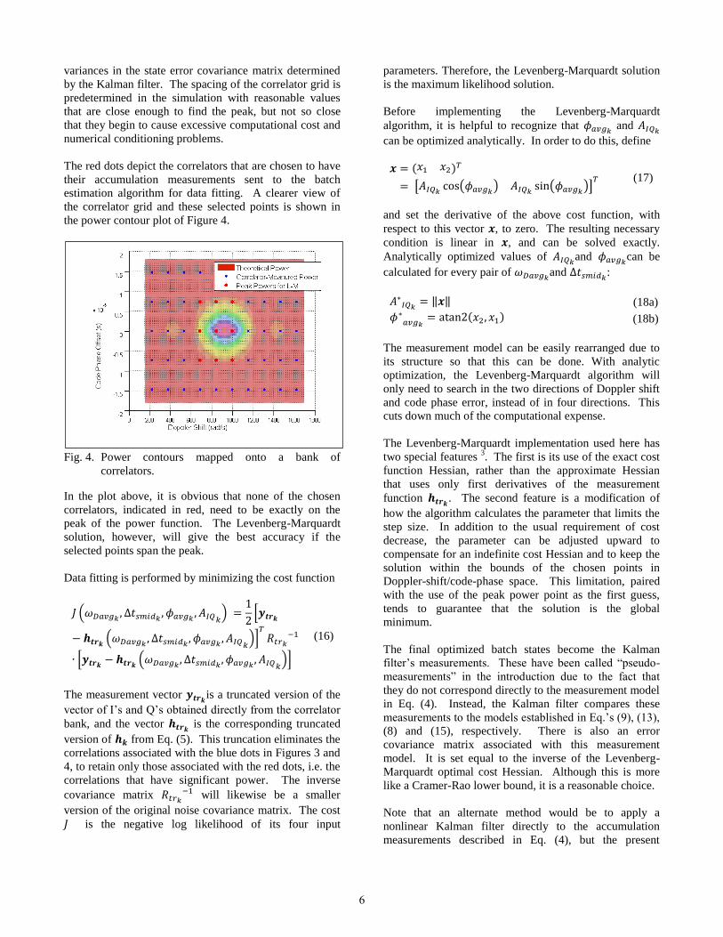
The red dots depict the correlators that are chosen to have

their accumulation measurements sent to the batch

estimation algorithm for data fitting. A clearer view of

the correlator grid and these selected points is shown in

the power contour plot of Figure 4.

Fig. 4. Power contours mapped onto a bank of

correlators.

In the plot above, it is obvious that none of the chosen

correlators, indicated in red, need to be exactly on the

peak of the power function. The Levenberg-Marquardt

solution, however, will give the best accuracy if the

selected points span the peak.

Data fitting is performed by minimizing the cost function

(

)

*

(

)+

*

(

)+

(16)

The measurement vector is a truncated version of the

vector of I’s and Q’s obtained directly from the correlator

bank, and the vector is the corresponding truncated

version of from Eq. (5). This truncation eliminates the

correlations associated with the blue dots in Figures 3 and

4, to retain only those associated with the red dots, i.e. the

correlations that have significant power. The inverse

covariance matrix

will likewise be a smaller

version of the original noise covariance matrix. The cost

is the negative log likelihood of its four input

parameters. Therefore, the Levenberg-Marquardt solution

is the maximum likelihood solution.

Before implementing the Levenberg-Marquardt

algorithm, it is helpful to recognize that and

can be optimized analytically. In order to do this, define

( )

[ (

) (

)]

(17)

and set the derivative of the above cost function, with

respect to this vector , to zero. The resulting necessary

condition is linear in , and can be solved exactly.

Analytically optimized values of and

can be

calculated for every pair of and

:

‖ ‖ (18a)

( ) (18b)

The measurement model can be easily rearranged due to

its structure so that this can be done. With analytic

optimization, the Levenberg-Marquardt algorithm will

only need to search in the two directions of Doppler shift

and code phase error, instead of in four directions. This

cuts down much of the computational expense.

The Levenberg-Marquardt implementation used here has

two special features 3. The first is its use of the exact cost

function Hessian, rather than the approximate Hessian

that uses only first derivatives of the measurement

function . The second feature is a modification of

how the algorithm calculates the parameter that limits the

step size. In addition to the usual requirement of cost

decrease, the parameter can be adjusted upward to

compensate for an indefinite cost Hessian and to keep the

solution within the bounds of the chosen points in

Doppler-shift/code-phase space. This limitation, paired

with the use of the peak power point as the first guess,

tends to guarantee that the solution is the global

minimum.

The final optimized batch states become the Kalman

filter’s measurements. These have been called “pseudo-

measurements” in the introduction due to the fact that

they do not correspond directly to the measurement model

in Eq. (4). Instead, the Kalman filter compares these

measurements to the models established in Eq.’s (9), (13),

(8) and (15), respectively. There is also an error

covariance matrix associated with this measurement

model. It is set equal to the inverse of the Levenberg-

Marquardt optimal cost Hessian. Although this is more

like a Cramer-Rao lower bound, it is a reasonable choice.

Note that an alternate method would be to apply a

nonlinear Kalman filter directly to the accumulation

measurements described in Eq. (4), but the present

6

method has the advantage of increased accuracy by

“linearizing” about the parameters that give peak

accumulation power, instead of only linearizing about the

Kalman filter’s a priori estimate. The Levenberg-

Marquardt algorithm is also a way to transition between

the large collections of accumulations produced by the

correlator bank to a reasonable set of measurements that

the Kalman filter can easily incorporate.

VI. IMPLEMENTATION OF KALMAN FILTER

Two Kalman filters are tested for the tracking algorithm:

A nonlinear extended square root information filter (EKF)

and a nonlinear unscented Kalman filter (UKF). The

results from these two filters have no significant

difference. The Kalman filter makes use of the dynamic

models for carrier phase, carrier Doppler shift, rate of

change of carrier Doppler shift, carrier amplitude and

code phase error. This model is a combination of Eq.’s

(7), (12) and (14), and is used in dynamic propagation.

The model used for measurement update is the output of

the batch optimization, as described in the previous

section. Both processes of dynamic propagation and

measurement update are nonlinear due to carrier-aiding

being present in code phase dynamics. This nonlinearity

is the only one remaining after Levenberg-Marquardt, and

its weakness is likely the cause of the close similarity of

results produced by the different extended filters.

Also implemented within the Kalman filter are four data

tests that are used in order to decide whether or not to

perform a measurement update. All four tests must be

passed to perform an update. The first test accepts data

only if the peak accumulation power in the correlator

bank does not lie on a boundary in the Doppler shift or

code delay range. The second test requires that the

Levenberg-Marquardt algorithm converges in a

reasonable number of iterations. The third test examines

the optimal Leveberg-Marquardt cost. It should be half of

a chi-squared sample from a distribution of degree

, where

is the number of elements in

and in , or twice the number of selected red dots in

Figures 3 and 4. If the optimal Levenberg-Marquardt cost

is too high, say high enough that the random probability

of generating it is less than 10-4

, then the measurement is

rejected. The fourth test performs the Kalman filter

measurement update, and examines the value of the sum

of the squares of the normalized innovation vector. It

should be a sample from a chi-squared distribution of

degree four. If the value is too high, then the

measurement update is rejected. Such rejections,

however, are rare, except at very low carrier-to-noise

ratios.

VII. PLL AND DLL FEEDBACK CONTROL LAWS

Feedback control laws are needed in order to complete the

loop shown in Figure 2, by implementing the correlator

block control segment. These laws take the most recent

Kalman filter a posterior state estimates to predetermine

the accumulation intervals, the NCO carrier Doppler

shifts, as defined in Eq. (3a), and the NCO code phase

offsets, as defined in Eq. (3b). The feedback from a given

accumulation interval is used to set these values two

accumulation intervals forward.

The DLL feedback control law determines the k+2nd

accumulation interval as follows:

(19)

The effect of this control law is to use the code phase

offset estimate at , which is

, and the

predicted lengths of the k+1st and k+2

nd intervals, so that

the predicted code phase offset at will be zero.

The DLL also needs to predict the expected average code

phase error for the k+2nd

accumulation interval. Although

the expected error is zero at the end of the interval, as per

the design of Eq. (19), it is not necessarily zero at the

beginning. In fact, it equals half the sum of the first,

second and fourth terms on the right-hand side of Eq.

(19):

.

/

(

(20)

Eq. (3b) also requires a choice of the PRN code spacing

and the number of code offsets P. is normally

chosen in the range 0.5 to 1 code chip lengths. P is

normally chosen so that is four to six times the

Kalman filter’s 1-σ code phase uncertainty, as computed

from its covariance matrix. Note that a minimum value of

P = 3 is enforced when the code delay uncertainty is very

small.

The nominal Doppler shift predicted by the PLL for the

k+2nd

accumulation interval is

7

(

* (21)

Eq. (3a) also requires a choice of the Doppler shift

spacing and the number of Doppler offsets L.

is normally chosen in the range ⁄ to

⁄ , i.e. from ½ to 1 times the accumulation

frequency. L is normally chosen so that is four to

six times the Kalman filter’s 1-σ Doppler shift

uncertainty. Note, however, that a minimum value of L = 3 is always used, even when the Doppler shift uncertainty

is very small.

The “hat” accents denote estimates given by the Kalman

filter, for time . These do not become available

until shortly after that time, because they are based on

accumulations from the interval that ends at that time.

Presumably, the receiver’s processor can finish

computing all of these feedback quantities during the

interval from to

, so that they will be

available to the correlator block control segment during

the interval from to

.

VIII. LIMB SCAN SIMULATION

The rising-GPS-satellite limb-scanning application, with a

low-Earth orbit (LEO) satellite carrying a GPS receiver, is

an ideal application for this acquisitionless tracking

system. The most useful meteorological data occurs just

at the initial point when the satellite rises, but it is difficult

to start tracking the signal immediately at this point with

traditional receiver algorithms. An acquisition would

waste some of this valuable data.

To investigate the new system’s performance on this

problem, a high-fidelity truth-model simulation of a limb

scan has been developed. Its goal is to show that the new

Kalman Filter can start tracking the signal with high

accuracy on its carrier and code phase, immediately upon

availability. Thus, meteorological data could be captured

for limb scans with minimum altitudes of only several

meters.

The truth-model simulation includes LEO orbital

dynamics, namely, a circular orbit with 700 km of altitude

and 98.2° of inclination. The GPS satellite orbital

dynamics are modelled using standard GPS ephemerides

and orbit calculations. As the orbital dynamics cause the

signal to penetrate the atmosphere, the signal path

experiences refraction dictated by the generalized 3D

Snell’s law differential equation, and through modelled

neutral atmosphere density and ionosphere electron

density distributions. The solution for the refracted path

is that of a two-point boundary value problem (TPBVP)

between each LEO and GPS satellite location. Figure 5

renders an example of a curve determined by the TPBVP

solver. The plot shows the geometry of the Earth limb

(blue), the straight-line path (green) which is occulted,

and the refracted bent path (red) which has a minimum

altitude of 54 m.

Fig. 5. Sketch of limb-scan geometry.

The effects on carrier Doppler shift and pseudorange are

calculated at discrete time points and then interpolated

between these times. These effects are due to

tropospheric and ionospheric refraction, and cause large

initial perturbations in pseudorange and Doppler shift, as

shown in Figure 6. The modelled refraction includes the

phenomena of geometric path bending, signal group-

delay/phase-delay in the troposphere, and group-

delay/phase-advance in the ionosphere.

Fig. 6. Pseudorange and carrier Doppler shift

perturbation time histories due to refraction.

The change in Doppler shift in the first 20 seconds is

about 300 Hz, translating into an apparent unmodelled

acceleration of about 0.3 g at the L1 carrier frequency.

The initial pseudorange offset is 1040 m, which implies a

code phase uncertainty of about 3.5 chips of C/A code.

The effects of receiver clock error are also simulated

using a standard Markov model. They are given in Ref. 4.

IX. SIMULATION TESTING RESULTS

The following are results of applying the new algorithm

to the limb-scan truth-model simulation. The overall

simulation has been implemented in MATLAB and uses

8

correlator grid spaces of 37.5 Hz in Doppler

shift and 0.75 chips in code phase offset. These

are reasonable, albeit ad-hoc, values that are large enough

to avoid numerical issues such as poor conditioning of

noise covariance matrices. The receiver clock model uses

the parameters 10-22

s and 7.6×10-24

s-1

.

These clock parameters yield a minimum root Allen

variance of 10-11

at a delay of 1 s, consistent with an

ovenized crystal oscillator. is set to 140 rad2/s

5; this

value is based on measures of the degree of error between

“truth” phase and the rate at which it deviates from a

quadratic in the limb-scan time histories. The nominal

model accumulation interval is set to 0.02 s, giving

50 Hz accumulations. The carrier frequency

corresponds to that of the L1 signal.

Figure 7 plots the simulated time history of carrier

Doppler shift, from the point that the GPS satellite rises

above the Earth limb, as viewed by the LEO satellite. It is

important to consider not only the speed with which the

PLL achieves lock, but also its successful pull-in from an

initial Doppler shift offset of 122 Hz, despite using 50 Hz

accumulations. These conditions would prevent a

traditional 2- or 3-correlator from ever achieving lock.

Fig. 7. Time history of carrier Doppler shift.

Similar results are seen for PRN code phase error, shown

in Figure 8. The DLL also achieves and maintains lock

very quickly, even with an initial code phase error of 5

chips. Uncertainty is plotted in the form of a 1-σ value,

which also drops nearly to zero after only about 0.03 s.

The simulated carrier-to noise ratio and its estimate are

shown in Figure 9. The signal starts with about 15 dB of

attenuation due to atmospheric path loss and the effects of

refractive lensing. This power loss disappears after 60 s,

by which time the signal path is largely clear of the

atmosphere. The congruence of the “truth” and estimated

C/N0 plots implies that signal amplitude is also being

tracked effectively.

Fig. 8. Time history of PRN code phase error.

Fig. 9. Time history of carrier-to-noise ratios.

The final signal parameter of interest is carrier phase. Its

error time history is graphed in Figure 10. Note once

again that within about three accumulation intervals, the

phase error is pulled in from a full cycle to a few degrees.

The ±1-σ uncertainty is effectively infinite at filter

initialization, but it decreases to a very small value within

the first few accumulation intervals.

Fig. 10. Time history of carrier phase error.

9

The algorithm responds to the aforementioned drops in

uncertainty by lowering the number of correlators that

must be used, saving computational cost. Time histories

of these numbers are shown in Figure 11. The bank of

correlators starts with L = 21 NCO Doppler shifts and P = 21 different NCO code phase offsets. The equality of the

numbers is largely a coincidence resulting from initial

uncertainty ranges.

Fig. 11. Time history of correlator bank size.

The rapid reductions in uncertainty, as indicated by the

Kalman filter covariance matrix, translate into drops in

the numbers of NCO grid points both in the Doppler shift

offset direction and in the code offset direction. After a

short time, only three correlators are used in each

direction to maintain lock.

CONCLUSION

A new GPS signal tracking algorithm has been developed

to combine PLL and DLL functions with accumulation

data from acquisition-like correlator banks. Its purpose is

to achieve rapid tracking with large pull-in regions,

without the need for a separate initial acquisition. The

new tracking algorithm chooses the correlator with the

highest accumulation power from the bank of correlators,

along with some of its close neighbours in Doppler shift

and code phase offset. The accumulation measurements

from these selected correlators are passed onto a batch

nonlinear optimization method, an intermediate step to the

Kalman filter that retrieves the most likely signal

parameters. The Kalman filter treats the optimized batch

states as measurements and provides the PLL and DLL

control laws with the necessary inputs for defining the

region that must be covered by the bank of correlators.

The algorithm’s use of acquisition-like data enables it to

achieve robust tracking in the presence of highly dynamic

signals with large initial uncertainties. For example, PLL

pull-ins from 122 Hz of initial Doppler error can be

achieved using 50 Hz accumulations, as can DLL pull-ins

of from an initial error of 5 C/A code chips. This

capability may be very useful in tracking the signal from a

rising GPS satellite, received aboard a LEO platform.

The resulting limb-scan data, because near-instantaneous

tracking can be achieved, will provide information about

meteorological conditions within a few meters of the

Earth’s surface.

REFERENCES

1. Misra, P., and Enge, P., Global Positioning System:

Signals, Measurements, and Performance, Ganga-

Jamuna, (Lincoln, 2006), pp. 431-492.

2. Psiaki, M.L., and Jung, H., “Extended Kalman Filter

Methods for Tracking Weak GPS Signals,” Proc.

ION GPS 2002, Sept. 24-27, 2002, Portland, OR, pp.

2539-2553

3. Gill, P.E., Murray, W., and Wright, M.H., Practical

Optimization, Academic, (London, 1981), pp. 136-

137.

4. Brown, R.G., Hwang, P.Y.C., Introduction to

Random Signals and Applied Kalman Filtering, J.

Wiley, (New York, 1992), pp. 428-432.

10