gms tutorials lidar v. 10 - amazon s3

GMS Tutorials Lidar

of 13 © Aquaveo 2020

GMS 10.5 Tutorial

Lidar Using lidar for interpolation and visualization in GMS

Objectives This tutorial teaches how lidar data can be used in GMS for display and interpolation.

Prerequisite Tutorials Getting Started

Required Components GIS Module

Time 10–20 minutes

v. 10.5

GMS Tutorials Lidar


1 Introduction ................................................................................................................... 2 1.1 Getting Started ........................................................................................................ 2

2 Importing Lidar Data .................................................................................................... 3 3 Lidar Display Options ................................................................................................... 4

3.1 Filtering Lidar ........................................................................................................ 5 3.2 Contours ................................................................................................................. 6 3.3 Color by classification ............................................................................................. 6 3.4 Number of points displayed ..................................................................................... 7 3.5 Bounding box ......................................................................................................... 7 3.6 Trimming Lidar ...................................................................................................... 8

4 Exporting a Filtered Lidar ............................................................................................ 9 5 Converting Lidar to a Raster ...................................................................................... 10 6 Interpolate Lidar to a UGrid ...................................................................................... 11 7 Filling holes when interpolating .................................................................................. 13 8 Multiple Lidar Files..................................................................................................... 13 9 Conclusion .................................................................................................................... 13

1 Introduction

Lidar stands for Light Detection and Ranging. A lidar file typically contains many 3D

points representing features on the Earth’s surface.

Lidar data can be used in GMS for display and interpolation to other objects. A number of

features exist to efficiently handle the large amount of data that is typical with lidar, such

as options to display a subset of points and exclude points. To maintain efficiency,

individual points cannot be selected or edited.

In this tutorial, a lidar file representing the area around Boulder, Colorado, will be

imported and used in various ways. Topics covered include:

Importing a lidar file

Filtering lidar

Changing the display options

Exporting lidar

Interpolating to ugrids

Creating a raster from a lidar file

1.1 Getting Started

Do the following to get started:

1. If necessary, launch GMS.

2. If GMS is already running, select File | New to ensure that the program settings

are restored to their default state.

GMS Tutorials Lidar


2 Importing Lidar Data

Start with opening a file containing lidar data. Lidar data is typically very dense and the

files can be very large.

1. Click Open to bring up the Open dialog.

2. Browse to the Tutorials\GIS\lidar directory

3. Select “Raster/DEM Files” from the Files of type drop-down and select “22.las”.

4. Click Open to close the Open dialog.

The Graphics Window should appear similar to Figure 1. This is a lidar of almost one

million points located near Boulder, Colorado. Only 50,000 points are being displayed due

to the current display options. Notice in the status bar in the bottom right of the GMS

window, the projection is being displayed. The projection information was included in the

lidar file and GMS set the display projection to match it. For more information on

projections, refer to the “Projections” tutorial.

Figure 1 LiDAR data in GMS

5. Zoom in and out on the raster using the mouse wheel or Zoom . If zooming in

far enough, individual points can be seen as in Figure 2.

6. When done zooming in, click on the Frame macro.

GMS Tutorials Lidar


Figure 2 Lidar points

3 Lidar Display Options

Each lidar file has its own display options. This differs from how GMS works with most

other objects. The lidar display options are accessed by right-clicking on the lidar items in

the Project Explorer.

1. Right-click on “ 22.las”, and then select Display Options… to bring up the

Lidar Display Options – 22.las dialog.

Figure 3 Lidar Display Options dialog

GMS Tutorials Lidar


3.1 Filtering Lidar

Lidar use classifications and return types for each point, signifying a possible trait the

points have. The classifications have been given a name based on possible terrain types,

however they may not actually represent the given name. It is possible to filter out points

from the display that do not meet certain criteria. On the right side of the dialog, there is an

Exclude by section. Notice that it currently has Classification selected. Below this section

is a table listing each existing classification. Notice that each classification is currently

checked except “Low Point (Noise)”.

1. Check “Low Point (Noise)”.

2. Click Apply. If necessary, move the dialog to the side so the graphics window can

be seen.

The display should now look something like Figure 4. Notice that by including the extreme

values the contour coloring provides a less interesting picture. Note that by turning off the

“Low Point (Noise)” points they will not be used if interpolating from “ 22.las”. By

default, extreme values are not displayed when import a lidar file.

Filtering affects the points that are used when interpolating from lidar.

Figure 4 LiDAR data filtering out one classification

3. Uncheck “Low Point (Noise)” to return to the previous display options.

4. In the Exclude by section, click Return Type. Notice that the table below changes.

5. Check Second but not-last then click Apply.

The display should now look similar to Figure 5.

GMS Tutorials Lidar


Figure 5 LiDAR data filtered by a return type

6. Change the filter back to Classification and click Apply to return to the original

display options.

3.2 Contours

1. In the Points section, make sure that Contours is selected.

2. Click the Options… button next to Contours to open the Dataset Contour

Options – Lindar – 22.las dialog.

The lidar contour options are the same contour options that are used throughout GMS,

although some things are disabled.

3. Click Color Ramp… to open the Color Options dialog.

4. Click the Reverse button.

5. Click OK to close the Color Options dialog.

6. Click OK to close the Dataset Contour Options – Lindar – 22.las dialog.

7. Click Apply in the Lindar Display Options – 22.las dialog.

Notice that the contours are still visible, but now red is used for the maximum value

instead of the minimum value.

3.3 Color by classification

Now to look at assigning classification specific colors:

1. Select Color by classification.

GMS Tutorials Lidar


2. In the table on the right of the dialog, change the color of “Unclassified” to green,

“Ground” to brown, and “Water” to blue.

3. Click Apply.

The display should now look similar to Figure 6.

Figure 6 Points colored by classification.

3.4 Number of points displayed

Notice that the Total number of points in file is more than the Number of points

displayed. Because lidar files typically have a lot of points, GMS only displays the number

of points specified in order to speed up the display of the lidar file. However, when the

lidar is used as an interpolation source, GMS uses all the points in the file, not just those

being displayed.

The number of points displayed does NOT affect the points used when

interpolating from lidar.

1. Change the Max number of points displayed to 100,000 and click Apply.

Notice there are more points being displayed.

3.5 Bounding box

With some files, it can be hard to identify the extents of the lidar. To resolve this issue:

1. Check the box marked Show bounding box.

2. Click OK to close the Lidar Display Options – Lindar – 22.las dialog.

3. Click Oblique View .

GMS Tutorials Lidar


Notice that this created a box around the extents of the lidar. The box style can be changed

by clicking the Options… button next to the Show bounding box option.

3.6 Trimming Lidar

Sometimes the lidar covers an area much larger than the area of interest. We can trim the

lidar to the area of interest. Note that when a trimmed lidar is used as an interpolation

source, only the trimmed area is used.

Trimming affects the points that are used when interpolating from lidar.

1. Switch to Plan View .

2. Zoom in on the right side of the points as shown in Figure 7

Figure 7 Zoomed in on right side.

3. Return to the Lidar Display Options – Lindar – 22.las dialog by right-clicking on

“ 22.las” in the Project Explorer and selecting the Display Options…

command.

4. In the upper-right corner, check Exclusion extents, then click the Options…

button next to it to being up the Lidar Exclusion Extents dialog.

5. Check on the X/Y option.

6. Click the Update button. This sets the Min and Max values in the table.

The Update button gets the X and Y extents of the current view and updates the values in

the table below. For the Update button to work, the display must be in plan view. The min

and max X,Y and Z values can also be edited manually if desired.

GMS Tutorials Lidar


7. Click OK to close the Lidar Exclusions Extents dialog.

8. Click OK to close the Lidar Display Options – Lindar – 22.las dialog.

9. Switch to Oblique View .

Notice the lidar extents have been trimmed and the display should look something like

Figure 8.

Figure 8 Trimmed lidar.

4 Exporting a Filtered Lidar

GMS can export a filtered lidar file. The exported file will only include the filtered points.

1. Right-click on “ 22.las”, and click Export… to open the Lidar File dialog.

2. Enter “22_filtered” for the File Name.

3. Click Save to close the Lidar File dialog and export the lidar file.

If desired, the file could be changed this using the drop-down menu, and saved as a *.laz

file (compressed). A *.laz file is the same as a *.las file but compressed.

4. Click the New macro.

5. Select Don’t Save at the prompt.


7. Select “Raster/DEM Files” from the Files of type drop-down.

8. Select the “22_filtered.las” file and click Open.

GMS Tutorials Lidar


The display should appear similar to Figure 9.

Figure 9 Filtered lidar

9. Right-click on “ 22_filtered.las”, and then select Display Options to bring up

the Lidar Display Options –22filtered.las dialog.

Notice in the Classification table “Low Point (Noise)” is no longer present, because when

exporting the previous lidar file, “Low Point (Noise)” was filtered out.

10. Click Cancel to close the Lidar Display Options –22filtered.las dialog.

5 Converting Lidar to a Raster

Lidar data can be converted into a raster. Unlike lidar, rasters are uniformly gridded data.

Since rasters can also be used as a source of interpolation, it can be useful to convert the

lidar to a raster that has fewer data points and then use the raster for interpolation

thereafter. In this case, the raster would use less memory and would draw faster than the

lidar.

Convert a lidar to a raster by doing the following:

1. Right-click on “ 22_filtered.las”, then click Interpolate To | Raster… to open

the Interpolate Lidar to Raster dialog.

2. Change the Cell size to “10”.

Notice that the cells (X Y) boxes changed their values to fit the Cell size.

3. Click OK to close the Interpolate Lidar to Raster dialog and open the Raster File

dialog.

GMS Tutorials Lidar


4. Click Save to close the Raster File dialog without changing the default filename.

5. Uncheck “ 22_filtered.las” in the Project Explorer.

The raster now in the display should look similar to Figure 10.

Figure 10 Raster converted from Lidar

6 Interpolate Lidar to a UGrid

Lidar can be interpolated to a Ugrid. Start with importing a 2D UGrid.

1. Turn off “ 22_filtered.tif” and turn on “ 22_filtered.las” in the Project

Explorer.


3. Select “All Files (*.*)” from the Files of type drop-down.

4. Select the “ugrid.vtu” file and click Open.

This is a 2D grid that is in a location where a groundwater model will be created.

5. Right-click on “ 22_filtered.las” in the Project Explorer and click Interpolate to

| UGrid to open the Interpolate Lidar to UGrid dialog.

The target UGrid can be specified but it should already be set to the one that was just

opened so it does not need to be changed. The lidar can be interpolated to either the UGrid

points (cell corners) or to the cell centers. The area average radius defines a square

surrounding each point being interpolated to, with the length of each square side equaling

twice the radius. The lidar points found within each box are averaged to determine the

interpolated value at the UGrid point, as shown in Figure 11.

GMS Tutorials Lidar


Figure 11 Area average radius defining boxes around cell centers.

6. Select Cell centers in the Target dataset location section.

7. Click OK to close the Interpolate Lidar to UGrid dialog.

Notice that a new dataset appeared under “ ugrid” in the Project Explorer, titled “

22_filtered”. To see the interpolated values of the UGrid, turn on contours for the UGrid.

8. Click the Display Options macro to open the Display Options dialog.

9. Select “UGrid: ugrid – [Active]” from the list on the left.

10. Check on Face contours.

11. Select Options… next to Face contours to bring up the Dataset Contour Options

– Ugrid – 22_filtered dialog.

12. Select “Block Fill” from the Contour method drop-down.

13. Click OK to close the Dataset Contour Options – Ugrid – 22_filtered dialog.

14. Click OK to close the Display Options dialog.

15. Turn off “ 22_filtered.las”.

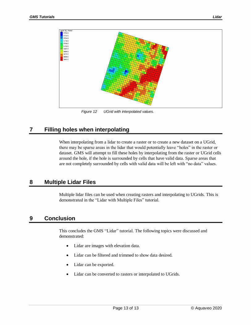
The display should now look something like Figure 12.

GMS Tutorials Lidar


Figure 12 UGrid with interpolated values.

7 Filling holes when interpolating

When interpolating from a lidar to create a raster or to create a new dataset on a UGrid,

there may be sparse areas in the lidar that would potentially leave “holes” in the raster or

dataset. GMS will attempt to fill these holes by interpolating from the raster or UGrid cells

around the hole, if the hole is surrounded by cells that have valid data. Sparse areas that

are not completely surrounded by cells with valid data will be left with “no data” values.

8 Multiple Lidar Files

Multiple lidar files can be used when creating rasters and interpolating to UGrids. This is

demonstrated in the “Lidar with Multiple Files” tutorial.

9 Conclusion

This concludes the GMS “Lidar” tutorial. The following topics were discussed and

demonstrated:

Lidar are images with elevation data.

Lidar can be filtered and trimmed to show data desired.

Lidar can be exported.

Lidar can be converted to rasters or interpolated to UGrids.

gms tutorials lidar v. 10 - amazon s3

Documents