glover
TRANSCRIPT

Sovereign Debt Crises and International Financial
Contagion: Estimating Effects in an Endogenous
Network
Brent Glover∗
Carnegie Mellon University
Seth Richards-Shubik†
Carnegie Mellon University
September 2012PRELIMINARY
Abstract
In an integrated global financial system, a sovereign default raises concerns of financial
contagion to other countries. We develop and estimate an equilibrium model featuring
a network of international borrowing and lending. In the model, the network structure
of borrowing-lending relationships arises endogenously and results in the propagation
of financial shocks across countries. We estimate the model using data on foreign claims
among a network of 20 countries over six years. Simulating counterfactual experiments
from the estimated model, we find a non-trivial role for financial contagion. The default
of a sovereign in the network has a noticeable effect on the borrowing costs and default
probabilities of other network members.
∗E-mail: [email protected]†E-mail: [email protected]

1 Introduction
The recent sovereign debt crisis in Europe has renewed concerns of financial contagion. In an
integrated global financial system, where countries are simultaneously borrowing and lending
from one another, the default of one country can directly result in the subsequent default of
its lenders. This linkage introduces the possibility of financial contagion, whereby the default
of one sovereign borrower can impair the financial position of its counterparties, leading to a
clustering of defaults. Such a crisis can have damaging effects on the real economic activity
of both the defaulting and non-defaulting countries.
In this paper we develop and estimate an equilibrium model of international borrowing
and lending in a network of large economies. In the model, countries finance a portion
of their capital investment by borrowing from other countries. These bilateral lending-
borrowing relationships between countries comprise an endogenous network where countries’
financial conditions are interconnected. In such a network, contagion risk arises naturally
as a shock to one sovereign can propagate through the network to generate a sovereign debt
crisis affecting multiple countries in the network.
Using data on foreign claims from the Bank for International Settlements, we estimate
the model for a network of 20 countries. In contrast to most of the existing literature on
contagion that takes financial networks as exogenous, the network structure in our model
arises endogenously as an equilibrium outcome. The lending-borrowing network evolves over
time in response to local economic shocks and the global supply and demand for capital.
With the estimated model parameters, we also conduct a series of counterfactual ex-
periments. These experiments provide us with an estimate of the degree of contagion risk
1

present in the existing network of international borrowing and lending. In particular, we do
this by simulating the default of a given country and examining the impact on the default
probabilities of other countries in the network. As a starting point, we consider a global econ-
omy with risk-neutral agents in which countries’ output shocks are uncorrelated. Simulating
counterfactual defaults in the estimated network, we observe contagion effects following the
default of a sovereign in the network. The fact that the estimated model is able to produce
these effects under this simplified environment suggests a significant role for contagion in
sovereign debt markets, even in the absence of an explicit amplification mechanism.
Our approach makes possible further analyses that will be added in an upcoming version
that extends this preliminary draft. First, we will simulate outcomes under counterfactual
network structures. That is, we will simulate the estimated model under alternative network
topologies and examine how the degree of contagion risk varies. Second, we will simulate
longer-run effects on investment and output, by solving for the complete lending-borrowing
network and projecting its evolution over time. In addition, if needed we can extend the
current empirical specification to allow for risk aversion and other nonlinearities by adopting
a simulation-based estimator.
Our paper is related to two existing strands of literature. The first is a relatively new
literature that studies financial networks and contagion. The second studies sovereign debt,
default, and credit risk, typically in the context of a dynamic general equilibrium model of
a small open economy.
The role of networks in financial contagion has been the subject of a growing literature
that mainly began with the theoretical work of Allen and Gale (2000) and Freixas, Parigi,
and Rochet (2000). Both papers model an interbank market where liquidity shocks from
2

consumers in different locations are the reason for interbank deposits and transfers. They
consider the possible contagion of insolvency throughout the system if one bank fails, and
both models indicate that more connected networks are more resilient against this contagion.
Allen and Babus (2009) provide a survey of the subsequent theoretical and empirical litera-
ture. As they note, several authors have found evidence of contagion in interbank networks,
although the network structures are taken as exogenous in these analyses.
Two recent papers attempt to endogenize the network structure, with certain restric-
tions. Babus (2009) models a network of interbank deposits among banks in one region with
common liquidity shocks, given pre-existing links with banks in another region that has the
opposite liquidity shocks. Assuming each bank is linked to every bank in the opposite region,
a network forms in the home region that minimizes the risk of contagion. Cohen-Cole, Pat-
acchini, and Zenou (2011) include a simple model of network formation in an empirical study
of interbank loans. They assume that banks move individually in an exogenous sequence,
and must either add or remove one link to maximize a myopic change in payoffs.1 To draw a
distinction with these papers, our model endogenizes the complete network of international
loans and treats this network in a unified fashion. Agents move simultaneously, and there is
no imposition of myopic beliefs.2
Relatively little work has considered the role of financial networks in spillovers from a
sovereign debt crisis, or other international contexts for financial contagion.3 The most
relevant to us is Bolton and Jeanne (2011), who develop a model that links government
1The use of an exogenous sequence of moves, and the myopic beliefs, are similar to Christakis et al. (2010)and Mele (2010). These assumptions function as equilibrium selection rules, with unclear consequences.
2Dynamic considerations do not impact behavior in our model, but this arises naturally from the primi-tives.
3Allen and Gale (2000) note that the different regions in their model could be interpreted as countries.
3

debt to the financial sector (where it is used as collateral for interbank loans). Sovereign
risk affects the reserves of domestic and foreign banks that hold this debt. With a simple,
two-country network, they show that banks diversify their debt portfolios, and so a sovereign
default in one country reduces liquidity, and hence investment and output, in both countries.
Empirically, a handful of recent papers provide evidence on the international transmission
of financial shocks during the recent financial crisis. De Haas and Van Horen (2011) and
Giannetti and Laeven (2011) examine international lending by large banks, and find that
those with greater losses or less access to credit made greater reductions in their cross-border
lending. Similarly, Cetorelli and Goldberg (2010) and Popov and Udell (2010) find that the
supply of loans fell in emerging markets due to reductions in cross-border lending from
international banks and local lending from banks with foreign parents, as well as reductions
in local lending by domestic banks affected by the international interbank market.
Our paper is also related to a literature that studies sovereign borrowing and lending.
This strand of literature builds on the seminal work of Eaton and Gersovitz (1981) to study
sovereign debt and default in a dynamic general equilibrium model. These papers study
sovereign borrowing with endogenous default in dynamic general equilibrium models with
incomplete markets. Arellano (2008) uses a quantitative model to study the interaction of
sovereign credit risk with output fluctuations and interest rates. A calibrated version of the
model is successful in matching Argentina’s business cycles statistics and the country’s 2001
default. Aguiar and Gopinath (2006) use a similar framework to study the quantitative pre-
dictions of a model of debt and default in a small open economy. They find a quantitatively
important role for a stochastic trend in growth rates for emerging economies. Arellano and
Ramanarayanan (2008) extend this framework of a sovereign borrower to allow for the choice
4

of debt maturity. They find a quantitatively important role for a sovereign’s choice of matu-
rity structure as it trades off the hedging benefits of long-term debt against the repayment
incentives induced by short-term debt. Borri and Verdelhan (2011) study the importance
of a risk averse lender in a model of sovereign borrowing. They show the importance of a
risk-averse lender, in this case with habit formation preferences, for matching the sovereign
bond yields observed in the data.
Finally, recent work in the finance literature has examined the time series properties and
comovement of sovereign credit risk by examining sovereign CDS spreads. Longstaff et al.
(2011) find that global factors explain a large portion of the common variation in sovereign
CDS prices. Dieckmann and Plank (2011) study CDS spreads for a sample of developed
countries and find strong comovement that increased significantly following the financial
crisis beginning in 2008. Pan and Singleton (2008) find that the spreads of Mexico, Turkey,
and Korea have a high correlation with volatility in the U.S. stock market as measured by
the VIX.
The remainder of the paper is organized as follows. Section 2 presents the network model
of international borrowing and lending. We discuss our empirical approach to estimating the
model in Section 3 and the data used in the estimation in Section 4. In Section 5 we present
the results from the estimated model. Finally, in Section 6 we use the estimated model to
simulate counterfactual sovereign defaults and examine the contagion effects of these shocks
propagating through the network of borrowing and lending relationships.
5

2 Model
We develop a representative agent model of macroeconomic investment and production,
international borrowing and lending, and solvency. Our model shares many features with
the existing literature, particularly Allen and Gale (2000) , Bolton and Jeanne (2011), and
Arellano (2008). However unlike some previous work on financial contagion or sovereign
debt crises, there is no separate banking sector or government sector. Instead, the agents in
our model function jointly as consumers, producers, and lenders.
The global economy consists of countries i = 1, . . . , N , which are of similar size.4 Each
country has a continuum of households, and these households have access to “projects” that
can convert an investment of the consumption good in one period into output in the next
period. Time is measured in discrete periods (t = 0, 1, 2, . . . ), with no terminal date. Given
an investment I in period t, a project yields f(I) in period t + 1, with f ′ > 0 and f ′′ < 0.
There is no other storage technology.
Households can make loans to invest in projects at other households, both in their own
country and in other countries. However they cannot invest in their own projects. This re-
striction generates lending and links financial activity to aggregate production in a relatively
simple macroeconomic model.5 Similar restrictions appear in other work, such as Bolton
and Jeanne (2011) where only some bankers have access to a project. A loan, l, made in one
period is paid back in the next period for a total return of rl, unless the recipient defaults
4We can instead allow countries to have different measures of households, µi, but this is omitted tosimplify the exposition. However no country is “small” relative to the global economy.
5It would be possible to remove this restriction, at the cost of other complications. For example, ifhouseholds were risk averse there would be an incentive to diversify by lending to other countries. Or wecould introduce competitive firms and have them manage the projects. These firms would need to distributetheir profits back to the households each period.
6

in which case there is some exogenous recovery rate (described later). Loans are made from
one particular household in country i to another household in country j (perhaps the same
country). However, we will restrict attention to symmetric equilibria, so we can usually
describe behavior in terms of one representative household in each country. In that case a
loan from country i to country j in period t is denoted ltij.
There is a cost of making loans to each country, given by a function c. It depends on
the total loans made by an individual household (h) to households in country j, lthij, and
the per capita amount of loans made by all households in the same country to country j in
the previous period: l̄t−1ij . The cost is increasing and convex in the individual household’s
current loans (lthij), which represents the difficulty of finding a good projects to invest in.
However there is a negative cross-partial with the per capita amount of loans made in the
previous period (l̄t−1ij ). This captures the idea that it is easier to find good projects in some
country if more households in your own country have invested there before. We use the per
capita amount rather than the household’s own lagged amount for convenience, because it
avoids a dynamic incentive to invest in order to reduce future costs. Still this assumption
can be motivated, in part, because good projects will appear at different households over
time, and so there may be a benefit in learning about these projects from other investors in
your country. To summarize, the cost of making loans to country j for some household h
in country i is c(lthij, l̄t−1ij ), with partial derivatives c1 > 0, c11 > 0, c12 < 0. In a symmetric
equilibrium we will have lthij = ltij and l̄t−1ij = lt−1ij , so this becomes c(ltij, lt−1ij )
Each period a household has revenues from its latest project and the return on its loans.
The total investment in the project at the representative household in country i in period
t − 1 is I t−1i =∑
j lt−1ji . Given this investment, the project yields f(I t−1i ) in period t. The
7
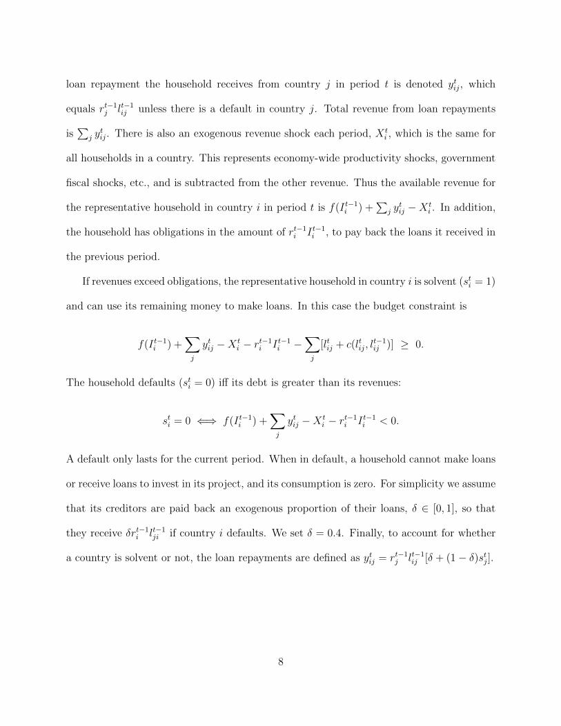
loan repayment the household receives from country j in period t is denoted ytij, which
equals rt−1j lt−1ij unless there is a default in country j. Total revenue from loan repayments
is∑
j ytij. There is also an exogenous revenue shock each period, X t
i , which is the same for
all households in a country. This represents economy-wide productivity shocks, government
fiscal shocks, etc., and is subtracted from the other revenue. Thus the available revenue for
the representative household in country i in period t is f(I t−1i ) +∑
j ytij −X t
i . In addition,
the household has obligations in the amount of rt−1i I t−1i , to pay back the loans it received in
the previous period.
If revenues exceed obligations, the representative household in country i is solvent (sti = 1)
and can use its remaining money to make loans. In this case the budget constraint is
f(I t−1i ) +∑j
ytij −X ti − rt−1i I t−1i −
∑j
[ltij + c(ltij, lt−1ij )] ≥ 0.
The household defaults (sti = 0) iff its debt is greater than its revenues:
sti = 0 ⇐⇒ f(I t−1i ) +∑j
ytij −X ti − rt−1i I t−1i < 0.
A default only lasts for the current period. When in default, a household cannot make loans
or receive loans to invest in its project, and its consumption is zero. For simplicity we assume
that its creditors are paid back an exogenous proportion of their loans, δ ∈ [0, 1], so that
they receive δrt−1i lt−1ji if country i defaults. We set δ = 0.4. Finally, to account for whether
a country is solvent or not, the loan repayments are defined as ytij = rt−1j lt−1ij [δ + (1− δ)stj].
8

2.1 Solution
A symmetric equilibrium is assumed. Given interest rates rtj, j = 1 . . . N , households in
country i choose loan amounts (ltij, j = 1 . . . N) and a level of debt and investment (I ti ) to
maximize consumption each period:
Cti = sti ·
(f(I t−1i ) +
∑j
ytij −X ti − rt−1i I t−1i −
∑j
[ltij + c(ltij, l̄t−1ij )]
).
Let pt+1i = Ets
t+1i be the equilibrium probability that the households in country i will be
solvent in the next period. Because the individual households are small, they cannot affect
default probabilities with their investment decisions, and so these probabilities are taken as
given as well. Expected consumption in the next period is
EtCt+1i = pt+1
i Et
(f(I ti ) +
∑j
yt+1ij −X t+1
i − rtiI ti −∑j
[lt+1ij + c(lt+1
ij , l̄tij)]|st+1i = 1
),
as consumption is zero when si,t+1 = 0. The optimization problem in period t is thus
maxIit,(lijt)
Cit + Et
∞∑s=1
ρsCt+si (1)
s.t. f(I t−1i ) +∑j
ytij −X ti − rt−1i I t−1i −
∑j
[ltij + c(ltij, l̄t−1ij )] ≥ 0.
(This includes a subjective discount rate ρ < 1 so that the objective is well defined.) To solve
this problem we only need to consider consumption in periods t and t + 1. This is because
an individual household cannot affect the per capita loan amounts, l̄tij, that affect costs and
hence lending in future periods. As a result, the optimization problem is in essence static.
The FOCs for loans involve the probability of default in the next period, both for the
lender and the debtor, because a loan is fully repaid and the lender benefits from this money
9

only if both are solvent. This can be seen from the expected benefit of a loan to country j,
which is
Et[ρst+1i yt+1
ij ] = ρpt+1i Et[r
tjltij[δ + (1− δ)st+1
j ]|st+1i = 1] = ρpt+1
i rtjltij[δ + (1− δ)pt+1
j|i ]
where pt+1j|i = Et[s
t+1j |st+1
i = 1] is the probability that the households in country j are solvent
conditional on those in i being solvent. Thus the marginal benefit is ρpt+1i rtj[δ + (1− δ)pt+1
j|i ]
while the marginal cost of a loan is 1 + c1(ltij, l̄
t−1ij ), and so the FOC is
ρpt+1i rtj[δ + (1− δ)pt+1
j|i ] = 1 + c1(ltij, l̄
t−1ij ) (2)
For loans within the same country, the expression is simpler because pt+1i|i = 1 (intuitively,
either all households will default or none will). So the expected benefit of a domestic loan is
pt+1i rtil
tii, and hence the FOC is ρpt+1
i rti = 1 + c1(ltii, l̄
t−1ii ).
The solvency probabilities, pt+1i , satisfy a system of equations:
pt+1i =
∫Y
FX
(f(I ti )− rtiI ti +
∑j
yt+1ij
)dFY (yt+1
i1 . . . yt+1iN ) (3)
where FX is the CDF of X and FY is the joint distribution of (yt+1ij ). The latter is derived
from the joint distribution of (X t+1j )Nj=1 because yt+1
ij = rtjltij · [δ + (1 − δ)st+1
j ], and st+1j is
determined as
st+1j = 1
{f(I tj)− rtjI tj +
∑k
yt+1jk −X
t+1j ≥ 0
}. (4)
As a result, computing (3) involves solving for s conditional on X and integrating over the
joint distribution of X.
10
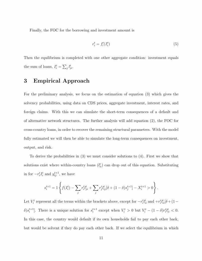
Finally, the FOC for the borrowing and investment amount is
rti = f ′i(Iti ) (5)
Then the equilibrium is completed with one other aggregate condition: investment equals
the sum of loans, I ti =∑
j ltji.
3 Empirical Approach
For the preliminary analysis, we focus on the estimation of equation (3) which gives the
solvency probabilities, using data on CDS prices, aggregate investment, interest rates, and
foreign claims. With this we can simulate the short-term consequences of a default and
of alternative network structures. The further analysis will add equation (2), the FOC for
cross-country loans, in order to recover the remaining structural parameters. With the model
fully estimated we will then be able to simulate the long-term consequences on investment,
output, and risk.
To derive the probabilities in (3) we must consider solutions to (4). First we show that
solutions exist where within-country loans (ltii) can drop out of this equation. Substituting
in for −rtiI ti and yt+1ij , we have
st+1i = 1
{f(I ti )−
∑j
rtiltji +
∑j
rtjltij[δ + (1− δ)st+1
j ]−X t+1i > 0
}.
Let V ti represent all the terms within the brackets above, except for −rtiltii and +rtil
tii[δ+(1−
δ)st+1i ]. There is a unique solution for st+1
i except when V ti > 0 but V t
i − (1 − δ)rtiltii < 0.
In this case, the country would default if its own households fail to pay each other back,
but would be solvent if they do pay each other back. If we select the equilibrium in which
11

the households pay each other back, this means the terms −rtiltii and +rtiltii[δ + (1− δ)st+1
i ]
will always cancel and can be removed from the expression. To gain further tractability, we
impose an additional equilibrium selection rule. Suppose that, given realizations of X t+1,
there are two solutions for st+1i and st+1
j : either both countries default or both are solvent.
In what follows, we always select the equilibrium where i and j remain solvent and pay
each other back. We apply this selection rule in determining pt+1j|i , pt+1
k|i,j and so on. In
principle these expressions can be derived all the way to pt+1z|−z, which is the probability that
country z will be solvent conditional on all the other countries being solvent. However in
the implementation we truncate the expansion used to compute pt+1i at three steps (i.e., up
to pt+1m|i,j,k). This is a reasonable approximation because each new step is discounted by 1−δ
σ,
so further steps would have little impact on the value of pt+1i .
We assume that the Xi shocks are independent across countries are independent across
countries and follow a conditional normal distribution. To account for hetereogeneity across
sovereigns, we assume that the standard deviation of a country’s shock scales in the size of
its economy, Zi. Specifically, each country’s shock, Xi, is conditionally normally distributed
as
X t+1i |X t
i ∼ N (−β0 − β1X ti , Z
2i σ
2)
Additionally, we allow for an intercept term equal to β0Zi. In what follows, we set Zi
to be a country’s (seasonally adjusted) GDP in the fourth quarter of 2004, the quarter
immediately preceding the beginning of our sample period. To complete the specification of
equation (3), we use a quadratic for the production function: f(I ti ) = α1Iti + α2(I
ti )
2. This
yields the following specification for a country’s solvency probability:
12
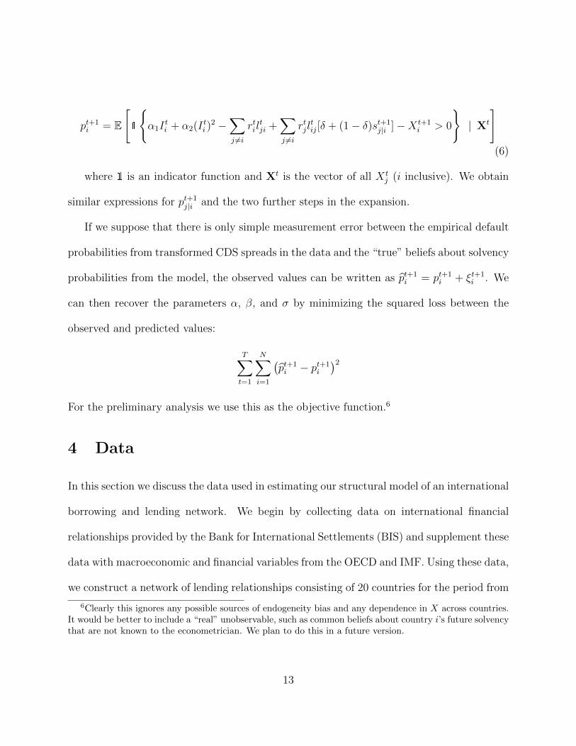
pt+1i = E
[1
{α1I
ti + α2(I
ti )
2 −∑j 6=i
rtiltji +
∑j 6=i
rtjltij[δ + (1− δ)st+1
j|i ]−X t+1i > 0
}| Xt
](6)
where 1 is an indicator function and Xt is the vector of all X tj (i inclusive). We obtain
similar expressions for pt+1j|i and the two further steps in the expansion.
If we suppose that there is only simple measurement error between the empirical default
probabilities from transformed CDS spreads in the data and the “true” beliefs about solvency
probabilities from the model, the observed values can be written as p̂t+1i = pt+1
i + ξt+1i . We
can then recover the parameters α, β, and σ by minimizing the squared loss between the
observed and predicted values:
T∑t=1
N∑i=1
(p̂t+1i − pt+1
i
)2For the preliminary analysis we use this as the objective function.6
4 Data
In this section we discuss the data used in estimating our structural model of an international
borrowing and lending network. We begin by collecting data on international financial
relationships provided by the Bank for International Settlements (BIS) and supplement these
data with macroeconomic and financial variables from the OECD and IMF. Using these data,
we construct a network of lending relationships consisting of 20 countries for the period from
6Clearly this ignores any possible sources of endogeneity bias and any dependence in X across countries.It would be better to include a “real” unobservable, such as common beliefs about country i’s future solvencythat are not known to the econometrician. We plan to do this in a future version.
13

2005Q1 to 2011Q3. Table I lists the countries included in our sample.
Figure 1 gives a representation of the lending network in 2011Q3, the last period in our
data. The arrows represent financial claims that one country has on another. These amounts
are normalized by the size of the economy of the lender country, using total GDP in 2004,
to reflect their relative exposure. Darker arrows indicate larger proportional amounts, and
claims worth less than one percent of the lender’s 2004 GDP are not shown. The darkest
arrows, which are from Switzerland (CH) to the United Kingdom (GB) and the United
States (US), from the United Kingdom to the United States, and from Ireland (IE) to the
United Kingdom (largely obscured), represent claims worth over 50% of the lender’s 2004
GDP. Nearly all countries have claims on each other, and so arrows can be bidirectional such
as between Austria (AT) and Italy (IT). Yet there are many unidirectional arrows because
often one country out of any pair has a relatively small amount of claims on the other.
The algorithm places more strongly connected countries in the center and more weakly
connected countries in the periphery.7 The US and UK are very large debtors when claims
are put relative to their creditors’ economies, so they are made quite central. Switzerland is a
very large lender relative to its own economy, France (FR) is both a moderately large lender
and debtor in the normalized amounts, and Germany (DE) is a fairly large debtor. Other
countries such as the Netherlands (NL) may serve as important “bridges” in the network
structure.
In addition to the lending relationships, we collect data on countries’ GDP, investment,
yields on government-issued long-term bonds, and prices on sovereign credit default swaps.
7However this is not a unique representation of the network, as it is a projection of an N by N matrixinto two dimensions. Different algorithms produce different visual representations, although the qualitativefeatures are reasonably stable.
14

The GDP and investment series for each country come from the OECD’s Quarterly National
Accounts dataset. Specifically, we use quarterly GDP growth rates and gross fixed capital
formation. The gross fixed capital formation is measured in fixed PPP and both series are
seasonally adjusted. Additionally, we collect yields on 10-year government bonds from the
OECD’s Monthly Monetary and Financial Statistics database.
In Table II we report the time series mean and standard deviation of each country’s
GDP growth, investment growth, and bond yield during the sample period. All statistics
are computed at a quarterly frequency over our sample period of 2005Q1 to 2011Q3. The
first column of the table indicates that all countries in our sample have a positive average
GDP growth over this period, however, there is significant heterogeneity in the average
growth rate and volatility of growth across countries. The third and fourth columns of the
table display the time series mean and standard deviation of the change in each country’s
investment. Again, we see significant heterogeneity in these values across the sovereigns in
our sample. The last two columns display the mean and standard deviation of each country’s
10-year government bond.
We collect CDS prices from Datastream for each country in our sample. The prices are
all for 5-year CDS contracts referencing the sovereign entity, with all contracts denominated
in US dollars. Table III displays summary statistics for the time series of CDS prices for each
of the sovereigns in our sample. We report the time series mean and standard deviation,
as well as the serial correlation of the monthly sovereign CDS prices. Comparing the first
and second columns of Table III, we see that the time series standard deviation exceeds the
mean for many sovereigns in our sample. In addition, the table shows that the sovereign
CDS prices exhibit a high degree of serial correlation.
15

Figure 2 plots the time series of the cross-sectional mean and quartiles of the sovereign
CDS prices in our sample. For each date, we compute the cross-sectional mean, median,
25th, and 75th percentiles of the sovereign CDS prices. Panel A displays the time series of
the mean and Panel B presents the quartiles. Beginning in 2008, we observe a susbstantial
rise in both the level and cross-sectional dispersion of CDS prices and this pattern continues
through the remainder of our sample.
In Table IV we present the matrix of pairwise correlations of the CDS prices for our sample
period. The table shows that nearly all of the sovereigns in our network have positively
correlated CDS prices and for many pairs of countries this correlation is strikingly high. To
further investigate the comovement of the sovereign CDS prices in our sample, we estimate
the first two principal components for our CDS price series. Panel A of Table V reports the
first two principal components estimated for the sovereign CDS prices for the countries in
our sample. The first principal component explains 64% of the variation in the sovereign
CDS prices and the first two principal components together explain 89% of the variation.
As a point of reference, we estimate the first two principal components for the government
long-term bond yields and GDP growth rates in our sample. These values are reported in
Panels B and C of Table V. The first principal component explains 60% and 63% of the
variation in government bond yields and GDP growth rates, respectively.
From these data, we construct the variables used in equation (6) as follows. Using the
5-year sovereign CDS spreads and the U.S. Treasury yield curve, we compute the time series
of quarterly solvency probabilities for each sovereign.8 For the gross returns on loans, rti ,
we directly use the yields on 10-year government bonds. The measure of baseline output,
8Note that this transformation of CDS spreads to solvency probabilities assumes a 40% recovery rate anda discount factor derived from the current Treasury yield.
16

Zi, is a country’s annual GDP in 2004, and investment, I ti , is quarterly gross fixed capital
formation.9 For the revenue shock, X ti , we use the quarterly GDP growth rate multiplied
by the baseline output. In addition the growth rate is first detrended by subtracting the
average quarterly growth rate from 1995 to 2004. For the amount of loans from one country
to another, ltij, we directly use the BIS data on foreign claims on an ultimate risk basis. While
these claims mostly have maturities longer than three months, the existence of secondary
markets means that claims do not have to be held until maturity. Lastly, as noted before,
we fix the exogenous recovery rate at δ = 0.4.
5 Results
The parameters recovered by our estimation procedure are listed in Table VI. The marginal
effect of international debts on a sovereign’s solvency probability is significant. A difference of
one unit in the normalized debt load is large, meaning a difference in total foreign claims on a
country equal to its annual GDP in 2004 (i.e.,∑
j 6=i ltjir
ti/Zi = 1). However the data span this
amount; for example, over our time period the total foreign claims on Austria, Ireland, and
Portugal all range by more than their GDP. At a point in time, the range of the normalized
debt load across countries is also greater than one in most quarters. The size of this marginal
effect is large relative to the average default probability: a one unit increase in the debt load
raises the quarterly default probability by approximately 105 bps. Alternatively, a net debt
increase of 85%, which is equal to one standard deviation of the normalized distribution,
amounts to a decrease of 89 bps in the sovereign’s solvency probability in the next quarter.
Other factors have significant estimated effects as well. A one percentage point increase
9All series are in US dollars (converted via fixed PPP) and seasonally adjusted where appropriate.
17

in a sovereign’s quarterly GDP growth results in a reduces the sovereign’s probability of
default in the next quarter by 40 bps. A one standard deviation change in the normalized
distribution of investment (which amount to a reduction in investment of 5% of a country’s
2004 Q4 GDP), results in a 82 bps decrease in the sovereign’s solvency probability in the
next quarter.
Figure 3 plots the observed and predicted solvency probabilities to illustrate the dis-
persion in the data and the model’s fit. In particular, we plot each sovereign’s observed
solvency probability, computed from its 5-year CDS spread, against the model predicted
solvency probability for each quarter in our sample. The values displayed are the probabil-
ity that a sovereign does not default in the next quarter. We can see that for most of the
observations, a country’s observed and predicted solvency probability are both close to 1.
However, the figure illustrates clear exceptions to this, most notably Greece, Ireland, and
Portugal. Generally, the model predictions match their counterpart empirical values rela-
tively well, as seen from the fact that most observations fall relatively close to the 45◦ line in
the plot. The model predictions appear to overestimate the solvency probability of Portugal
and Spain, relative to their empirical values, for some quarters, while it underestimates the
solvency probability of Ireland.
In Table VII, we present additional results on the distribution of solvency probabilities
as well as the fit of the model predicted probabilities with what is observed in the data for
our 396 observations. Panel A presents quartiles as well as the 5th and 95th percentile of
the distribution of quarterly solvency probabilities. The first column reports the empirical
solvency probabilities computed from the sovereign CDS spreads and the second column
presents the counterpart values predicted by the model under the estimated parameter values
18

given in Table VI. Panel B reports the correlation of the observed and model predicted
solvency probabilities as well as the sum of squared residuals. These values are 0.741 and
0.081, respectively.
6 Simulations
Using the estimated version of equation (6) we can simulate the short-run effect of a nation-
wide default on the solvency of other countries. The equation gives the probability that each
country will be solvent in the next quarter (i.e., period t + 1). To simulate the default of
some country j in that period, we replace the computed conditional probabilities pt+1j|i with
zero (and do the same for pt+1j|... in the second and third steps of the expansion). This makes
it so that the other countries receive no endogenous payments from country j, although they
still benefit from the exogenous recovery rate for a portion of their claims. The difference
between the original predicted solvency probabilities (pt+1i ) and the new predictions that
result from this change (p̃t+1i ) shows the increase in the default probabilities of the other
countries in period t + 1. This is a measure of the immediate contagious effect of a default
in one country.
We do this exercise separately for a default of Italy and a default of Spain using the last
period of our data (2011Q3), which means the simulated default occurs in 2011Q4. Table
VIII shows the total claims each country had on these two countries in 2011Q3, normalized
by the lender’s GDP in 2004. The largest lenders to Spain, relative to their own economies,
were the Netherlands and Portugal, both of which had claims worth over 10% of their annual
output. To Italy, the largest relative lender was France with claims worth over 20% of its
annual output.
19

The results of these simulations are in Tables IX and X. We focus our analysis on the
effect that a default by Spain or Italy would have on the other European sovereigns in
our sample. In the first column of each table, we present the absolute change, measured in
basis points, a sovereign’s default probability in the next quarter resulting from the default of
Italy (Table IX) or Spain (Table X). This change is measured relative to the model predicted
baseline in a case where the country does not default. The absolute magnitude of the baseline
quarterly default probability, even at the end of 2011, is relatively small for most sovereigns.
Therefore, the relative change in a sovereign’s default probability is also of interest as a small
absolute change in the default probability can still represent a significant relative change. To
this end, the second column of each table reports the relative increase, measured in percent,
in a sovereign’s one quarter default probability resulting from the default of Italy or Spain.
For both simulate default events, we observe significant heterogeneity in the response of
other sovereigns. Additionally, we see that a given country can have a significantly different
response to the two default events. For example, Portugal’s response to a default by Spain
is about an order of magnitude larger than its response to the default of Italy. Conversely,
we see that France would be more affected by Italy’s default than the default of Spain.
20

Table I:Country List
This table lists the countries included in our sample.
Country AbbreviationAustria ATAustralia AUBelgium BESwitzerland CHChile CLGermany DEDenmark DKSpain ESFinland FIFrance FRUnited Kingdom GBGreece GRIreland IEItaly ITJapan JPNetherlands NLPortugal PTSweden SETurkey TRUnited States US
21

Table II:Summary Statistics for Macroeconomic Variables
This table reports the mean, µ(·), and standard deviation, σ(·), for each country’s quarterly GDP growth
(∆y), investment growth (∆i), and long-term government bond yield (r) over the sample period 2005Q1 -
2011Q3. Further details regarding the data are provided in Section 4.
Country µ(∆y) σ(∆y) µ(∆i) σ(∆i) µ(r) σ(r)
Australia 0.68 0.54 1.53 2.55 5.48 0.49Austria 0.45 0.88 0.08 1.22 3.78 0.49Belgium 0.34 0.75 0.33 2 3.87 0.44Chile 1.06 1.27 2.24 5.32 5.29 2.3Finland 0.35 1.75 0.37 3.85 3.68 0.53France 0.23 0.62 0.18 1.52 3.71 0.47Germany 0.4 1.16 0.66 2.92 3.47 0.58Greece 0.06 1.22 -1.38 4.18 6.25 3.65Ireland 0.14 2.01 -2.79 8.55 5.13 2.03Italy 0.02 0.94 -0.35 1.77 4.28 0.48Japan 0.12 1.41 -0.48 1.78 1.42 0.24Netherlands 0.37 0.85 0.38 2.8 3.66 0.52Portugal 0.06 0.82 -0.95 2.6 4.9 1.9Spain 0.29 0.74 -0.73 2.52 4.16 0.58Sweden 0.55 1.32 0.7 2.89 3.47 0.55Switzerland 0.54 0.67 0.66 2.06 2.3 0.55Turkey 1.2 2.59 1.57 5.61United Kingdom 0.19 0.94 0.04 3.05 4.19 0.62United States 0.28 0.81 -0.42 2.46 3.87 0.74
Average 0.46 1.11 0.21 3.14 4.03 0.93
22

Table III:Summary Statistics for Sovereign CDS Prices
This table presents summary statistics for prices of 5-year Credit Default Swaps referencing the sovereign
entities in our sample. The columns labeled ‘Mean’ and ‘Std Dev’ display the time series mean and standard
deviation of the CDS price series. The autocorrelation of the monthly CDS prices is given in the column
labeled ‘AC(1)’. The final column reports the number of monthly observations available for each sovereign’s
CDS price series. All CDS prices are taken from Datastream.
Mean Std Dev AC(1) Min Max NAustria 47.8 58.9 0.95 1.5 235 100Australia 35.2 30.1 0.88 2.5 158.3 112Belgium 61.6 83.2 0.97 1.2 307.3 100Chile 64.9 55 0.92 7.8 254.2 100Germany 24 28.3 0.95 0.9 110.8 100Denmark 32.8 38.9 0.90 1.6 142 104Spain 115.6 134.4 0.97 2 462.5 85Finland 39 20.6 0.86 7.3 85.3 48France 48.5 57.4 0.98 1.5 214.7 81United Kingdom 63.8 31.7 0.92 7 147.3 54Greece 427.8 1020.3 0.92 5 6499.8 97Ireland 175.5 253.3 0.99 2 882.1 105Italy 97.6 127.3 0.97 5.6 485.4 100Japan 38.5 39.8 0.95 3 142.7 100Netherlands 36.6 35.9 0.91 1.2 120.8 80Portugal 208.4 363.9 0.98 2 1601 100Sweden 29.2 29.9 0.80 1.4 140 105Turkey 238.1 94.2 0.89 124.7 605.2 96United States 37.9 17.2 0.84 6.5 91.2 53Average 95.9 132.65 0.92 9.7 864.1 91
23

Tab
leIV
:C
orr
ela
tions
of
CD
SP
rice
s
Th
ista
ble
pre
sents
pai
rwis
eco
rrel
atio
ns
for
the
sove
reig
nC
DS
pri
ces.
Th
ed
ata
are
sam
ple
dat
am
onth
lyfr
equ
ency
for
the
per
iod
Janu
ary
2003
-A
pri
l20
12.
All
CD
Sp
rice
sar
eta
ken
from
Data
stre
am
.
Variables
Austria
Australia
Belgium
ChileGermany
Den
mark
Spain
Finland
France
U.K
.GreeceIreland
Italy
Japan
NetherlandsPortugalSwed
enTurkey
U.S.
Austria
1.00
Australia
0.91
1.00
Belgium
0.86
0.70
1.00
Chile
0.82
0.88
0.55
1.00
Germany
0.95
0.83
0.96
0.70
1.00
Den
mark
0.89
0.83
0.79
0.76
0.87
1.00
Spain
0.80
0.62
0.98
0.46
0.92
0.71
1.00
Finland
0.95
0.83
0.77
0.57
0.93
0.97
0.67
1.00
France
0.86
0.67
0.99
0.51
0.96
0.80
0.96
0.82
1.00
U.K
.0.86
0.85
0.51
0.73
0.72
0.75
0.44
0.72
0.51
1.00
Greece
0.63
0.44
0.81
0.31
0.76
0.63
0.74
0.64
0.86
0.30
1.00
Ireland
0.77
0.65
0.95
0.47
0.89
0.70
0.94
0.60
0.90
0.43
0.71
1.00
Italy
0.88
0.70
0.98
0.57
0.96
0.83
0.96
0.82
0.99
0.52
0.85
0.89
1.00
Japan
0.90
0.77
0.92
0.63
0.95
0.78
0.91
0.75
0.91
0.67
0.73
0.88
0.91
1.00
Netherlands
0.93
0.85
0.84
0.73
0.91
0.94
0.79
0.97
0.86
0.78
0.63
0.72
0.86
0.81
1.00
Portugal
0.72
0.53
0.93
0.36
0.86
0.71
0.92
0.66
0.94
0.30
0.88
0.91
0.94
0.85
0.72
1.00
Swed
en0.79
0.82
0.51
0.80
0.66
0.78
0.39
0.68
0.45
0.88
0.32
0.46
0.53
0.60
0.72
0.34
1.00
Turkey
0.20
0.30
-0.03
0.50
0.09
0.22
0.02
0.44
0.19
0.38
0.01
-0.10
0.01
-0.02
0.45
-0.08
0.25
1.00
U.S.
0.75
0.80
0.53
0.62
0.69
0.67
0.48
0.67
0.49
0.90
0.28
0.56
0.48
0.62
0.70
0.34
0.75
0.29
1.00
24

Table V:Principal Components Analysis
This table presents the first two principal components for the CDS prices (Panel A), 10-year bond yields
(Panel B), and GDP growth rates (Panel C), for the sovereigns in our sample. CDS prices are taken from
Datastream, bond yields are from the International Financial Statistics tables from the IMF, and GDP
growth rates are computed from the OECD’s quarterly national accounts.
Panel A: CDS PricesProportion Cumulative
Component 1 0.640 0.640Component 2 0.248 0.888
Panel B: Bond YieldsProportion Cumulative
Component 1 0.599 0.599Component 2 0.246 0.845
Panel C: GDP Growth RatesProportion Cumulative
Component 1 0.630 0.630Component 2 0.079 0.709
Table VI:Parameter Estimates
This table presents our main estimates of equation (6). The data and construction of the variables are
described in Section 4.
Parameter Valueα1 58.29α2 33.84β0 1.29β1 70.54σ 6.03
25
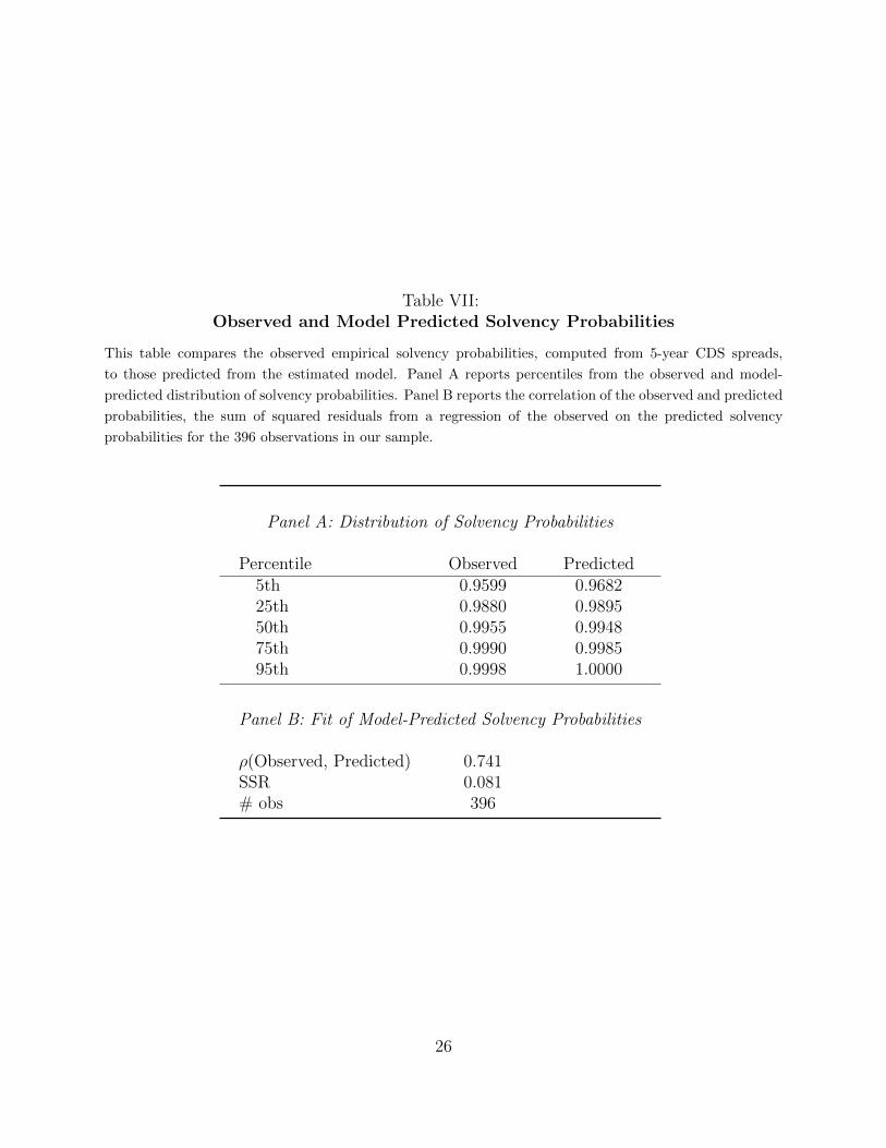
Table VII:Observed and Model Predicted Solvency Probabilities
This table compares the observed empirical solvency probabilities, computed from 5-year CDS spreads,
to those predicted from the estimated model. Panel A reports percentiles from the observed and model-
predicted distribution of solvency probabilities. Panel B reports the correlation of the observed and predicted
probabilities, the sum of squared residuals from a regression of the observed on the predicted solvency
probabilities for the 396 observations in our sample.
Panel A: Distribution of Solvency Probabilities
Percentile Observed Predicted5th 0.9599 0.968225th 0.9880 0.989550th 0.9955 0.994875th 0.9990 0.998595th 0.9998 1.0000
Panel B: Fit of Model-Predicted Solvency Probabilities
ρ(Observed, Predicted) 0.741SSR 0.081# obs 396
26
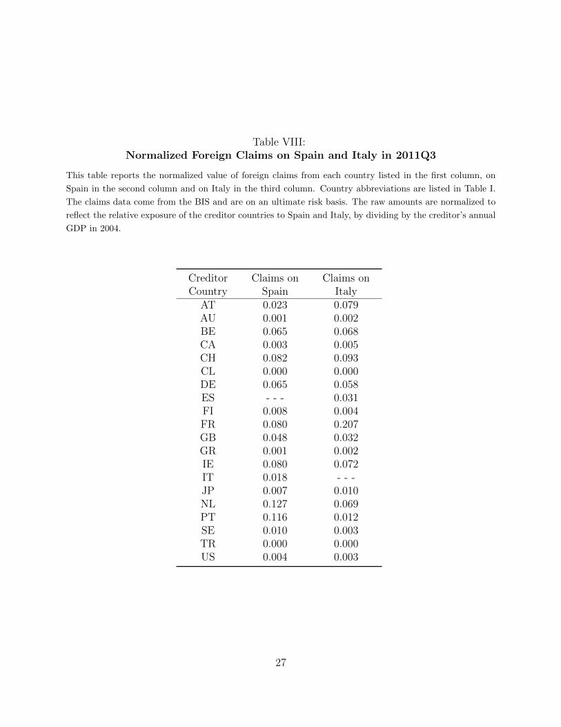
Table VIII:Normalized Foreign Claims on Spain and Italy in 2011Q3
This table reports the normalized value of foreign claims from each country listed in the first column, on
Spain in the second column and on Italy in the third column. Country abbreviations are listed in Table I.
The claims data come from the BIS and are on an ultimate risk basis. The raw amounts are normalized to
reflect the relative exposure of the creditor countries to Spain and Italy, by dividing by the creditor’s annual
GDP in 2004.
Creditor Claims on Claims onCountry Spain Italy
AT 0.023 0.079AU 0.001 0.002BE 0.065 0.068CA 0.003 0.005CH 0.082 0.093CL 0.000 0.000DE 0.065 0.058ES - - - 0.031FI 0.008 0.004FR 0.080 0.207GB 0.048 0.032GR 0.001 0.002IE 0.080 0.072IT 0.018 - - -JP 0.007 0.010NL 0.127 0.069PT 0.116 0.012SE 0.010 0.003TR 0.000 0.000US 0.004 0.003
27
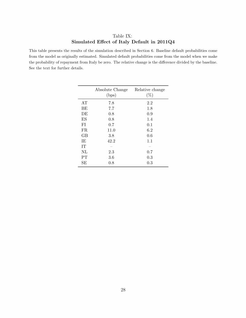
Table IX:Simulated Effect of Italy Default in 2011Q4
This table presents the results of the simulation described in Section 6. Baseline default probabilities come
from the model as originally estimated. Simulated default probabilities come from the model when we make
the probability of repayment from Italy be zero. The relative change is the difference divided by the baseline.
See the text for further details.
Absolute Change Relative change(bps) (%)
AT 7.8 2.2BE 7.7 1.8DE 0.8 0.9ES 0.8 1.4FI 0.7 0.1FR 11.0 6.2GB 3.8 0.6IE 42.2 1.1IT – –NL 2.3 0.7PT 3.6 0.3SE 0.8 0.3
28
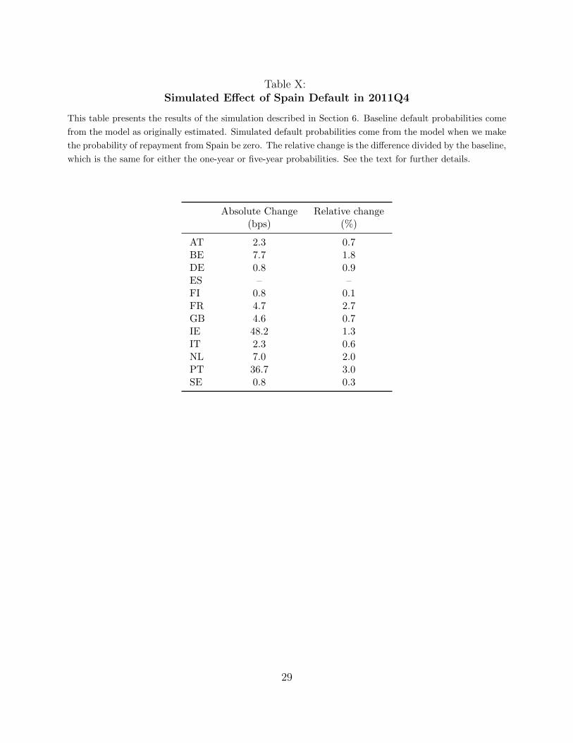
Table X:Simulated Effect of Spain Default in 2011Q4
This table presents the results of the simulation described in Section 6. Baseline default probabilities come
from the model as originally estimated. Simulated default probabilities come from the model when we make
the probability of repayment from Spain be zero. The relative change is the difference divided by the baseline,
which is the same for either the one-year or five-year probabilities. See the text for further details.
Absolute Change Relative change(bps) (%)
AT 2.3 0.7BE 7.7 1.8DE 0.8 0.9ES – –FI 0.8 0.1FR 4.7 2.7GB 4.6 0.7IE 48.2 1.3IT 2.3 0.6NL 7.0 2.0PT 36.7 3.0SE 0.8 0.3
29

Q3.2011
AT
BE
CH
CL
DE
ES
FI
FR
GBGR
IE
IT
JP
NL
PT
SEUS
Figure 1: Network Graph. This figure displays the network structure of lending relationships in thethird quarter of 2011. Countries are represented by their two letter abbreviation in Table I. Arrowsrepresent claims that one country has on another, and darker arrows indicate larger amounts inproportion to the creditor country’s GDP in 2004. For further description, see Section 4.
30

A. Mean CDS Price
Jan ’03 May ’04 Jul ’05 Oct ’06 Jan ’08 Apr ’09 Jul ’10 Oct ’110
100
200
300
400
500
600
Date
Avera
ge C
DS
Price
B. CDS Price Quartiles
Jan ’03 May ’04 Jul ’05 Oct ’06 Jan ’08 Apr ’09 Jul ’10 Oct ’110
50
100
150
200
250
300
350
400
Date
CD
S P
rice
Figure 2: Mean and Quartiles for CDS Prices. This figure plots the mean, median, and first andthird quartiles of the cross-section of the CDS prices for our sample of sovereigns. In Panel (A)the time series of the cross-sectional mean is plotted for January 2003-April 2012. Panel (B) plotsthe time series of the cross-sectional median CDS price (solid black line) along with the 25th and75th percentiles (blue dotted lines). All CDS prices are for 5-year CDS contracts referencing thesovereign entity. The sovereigns comprising our sample are listed in Table I.
31

0.85 0.90 0.95 1.00
0.85
0.90
0.95
1.00
Full Sample
Predicted
Obs
erve
d
AUBE
CLDEGR ITJPPTAT AUBE
CLDE ESGR ITJPPTSE AT
AUBECLDE ESFRGRIT JPNLPT
SEAT AUBECL
DE ESFRGR ITJPNL
PTSE
AT AUBECLDEESFRGR IEITJPNLPTSE AT AUBECLDEESFRGRIEITJPNLPTSEAT AUBECLDEESFRGR IEITJPNLPTSE ATAUBECLDEESFRGRIEITJPNLPTSE AT AUBECLDEESFRGR IEITJPNLPTSEAT AUBECLDEESFRGRIEITJPNLPT
SEAT AUBECLDEESFRGRIEITJPNLPT
SEAT AUBE
CLDEESFRGBGR IEITJPNLPTSE USATAUBE
CL
DEES
FRGBGR
IEITJPNL
PTSE USAT AUBE
CL
DEES
FRGBGR
IE ITJPNL
PTSE USAT AUBE
CL
DEES
FRGBGR IEIT
JPNLPTSE US
ATAU
BE
CL
DE
ES
FRGB
GRIE
IT
JPNL
PTSE
US
AT
AUBE
CL
DE
ES
FR
GB
GR
IE
IT
JPNLPTSE
USAT
AUBE
CL
DE
ES
FR
GB
GR
IE
IT
JPNLPTSE
USAT
AUBE
CL
DE
ESFR
GB
GRIE
ITJPNL
PTSEUS
ATAUBE
CL
DE
ES
FR
GB
GR
IE
ITJP
NL
PTSE
US
ATBECL
DE
ES
FRGB
GR
IEIT
JPNL
PT
SE USATBE CL
DE
ES
FI
FRGB
GR
IE
IT
JP
NL
PT
SE US
ATBE
CLDE
ES
FI
FRGB
GR
IE
IT
JPNL
PT
SE US
AT
BE
CLDE
ES
FI
FRGB
GR
IE
IT
JPNL
PT
SE USAT
BE
CLDE
ES
FI
FRGB
GR
IE
IT
JPNL
PT
SE USAT
BE
CLDE
ES
FI
FRGB
IE
IT
JP
NL
PT
SEUS
AT
BE
CLDE
ES
FI
FR
GB
IE
IT
JPNL
PT
SE US
Figure 3: Predicted and Observed Solvency Probabilities. This figure plots the predicted andobserved quarterly solvency probabilities for each country at each quarter in our sample. Theobserved solvency probabilities are obtained with a transformation of 5-year CDS contract prices,as described in Section 4. The predicted solvency probabilities are from the estimated version ofequation (6). Country abbreviations are listed in Table I.
32

References
Aguiar, M. and G. Gopinath. 2006. “Defaultable debt, interest rates and the current ac-
count.” Journal of International Economics 69:64–83.
Allen, F. and D. Gale. 2000. “Financial Contagion.” Journal of Political Economy 108 (1):1–
33.
Allen, Franklin and Ana Babus. 2009. “Networks in Finance.” The network challenge:
strategy, profit, and risk in an interlinked world :367.
Arellano, Cristina. 2008. “Default risk and income fluctuations in emerging economies.” The
American Economic Review 98 (3):690–712.
Arellano, Cristina and Ananth Ramanarayanan. 2008. “Default and the Maturity Structure
in Sovereign Bonds.” Working Paper .
Babus, Ana. 2009. “The Formation of Financial Networks.” Working paper .
Bolton, Patrick and Olivier Jeanne. 2011. “Sovereign default risk and bank fragility in
financially integrated economies.” IMF Economic Review 59 (2):162–194.
Borri, N. and A. Verdelhan. 2011. “Sovereign risk premia.” Manuscript, MIT .
Cetorelli, N. and L.S. Goldberg. 2010. “Global banks and international shock transmission:
Evidence from the crisis.” IMF Economic Review 59 (1):41–76.
Christakis, Nicholas, James Fowler, Guido Imbens, and Karthik Kalianaraman. 2010. “An
Empirical Model of Strategic Network Formation.” Working Paper.
33

Cohen-Cole, E., E. Patacchini, and Y. Zenou. 2011. “Systemic Risk and Network Formation
in the Interbank Market.” CEPR Discussion Papers .
De Haas, R. and N. Van Horen. 2011. “Running for the exit: international banks and crisis
transmission.” Working paper .
Dieckmann, S. and T. Plank. 2011. “Default Risk of Advanced Economies: An Empirical
Analysis of Credit Default Swaps during the Financial Crisis.” Review of Finance .
Eaton, J. and M. Gersovitz. 1981. “Debt with potential repudiation: Theoretical and em-
pirical analysis.” The Review of Economic Studies 48 (2):289–309.
Freixas, X., B.M. Parigi, and J.C. Rochet. 2000. “Systemic risk, interbank relations, and
liquidity provision by the central bank.” Journal of money, credit and banking :611–638.
Giannetti, M. and L. Laeven. 2011. “The flight home effect: Evidence from the syndicated
loan market during financial crises.” Journal of Financial Economics .
Longstaff, F.A., J. Pan, L.H. Pedersen, and K.J. Singleton. 2011. “How sovereign is sovereign
credit risk?” American Economic Journal: Macroeconomics 3 (2):75–103.
Mele, Angelo. 2010. “A Structural Model of Segregation in Social Networks.” Working Paper,
University of Illinois at Urbana-Champaign.
Pan, J. and K.J. Singleton. 2008. “Default and recovery implicit in the term structure of
sovereign CDS spreads.” The Journal of Finance 63 (5):2345–2384.
Popov, A. and G. Udell. 2010. “Cross-border banking and the international transmission of
financial distress during the crisis of 2007-2008.” ECB Working Paper No. 1203 .
34