1

Globalization in Developing Countries: The Role of

Transaction Costs in Explaining Economic Performance

in India

Maurizio BussoloOECD Development Centre

John WhalleyUniversity of Warwick

This version: September 2002

The quest for larger numbers for the impacts of trade liberalization has been going on for some timein international trade economics. This is because models of trade liberalization have consistentlyproduced results that, comparing ex post model results with real world data, show the right sign butthe “wrong” magnitudes. This means that the impacts of globalization in the form of tradeliberalization, on poverty is typically misspecified. This paper proposes a new approach byconsidering transaction costs reductions as an important factor explaining developing countries’ actualperformances. Under trade liberalization rather than presenting econometric estimates of transactioncosts from reduced form equations, this study explicitly introduces transaction costs in a system ofstructural form equations to build a general equilibrium simulation model. A clear mapping of theanalytical channels through which changes of transaction costs affect the economic results is thus aprimary objective. Additionally to the effect on aggregate income, the large number issue, this paperalso examines how transaction costs influence income distributional outcomes. Numerical simulationsbased on India are presented.

JEL Codes: D58, F11, F13, O10, O54Key Words: International trade, transaction costs, simulation models, income distribution

The views expressed in this paper are those of the staff involved and do not necessarily reflect those of theOECD Development Centre, and its member countries.

This paper forms part of the 'Exploring the Links Between Globalisation and Poverty in South Asia' study whichis part of the Globalisation and Poverty Programme, funded by the Department For International Development(DFID) UK. The Programme includes fourteen projects on a three-year programme of research exploring thelinkages between globalisation processes and poverty. DFID financial support is gratefully acknowledged.

2

1. Introduction

The quest for larger numbers for the impacts of trade liberalization has been going on for

some time in international trade economics. Numerical simulation models of trade

liberalization in multilateral, regional or single-country contexts have consistently produced

results that, compared ex post model analysis with real world data, show the right sign but the

“wrong” magnitudes. These quantitative assessments normally use core general equilibrium

models based on the theory of comparative advantage. The positive effects they are able to

measure originate from static resource reallocation improvements and the disappearance of

deadweight loss triangles. Unsatisfied by these meagre benefits estimates, economists have

built new models that explain better the large gains observed for internationally integrating

countries. Mainly they have gone into two directions, dynamics and non-convexities, i.e.

economies of scale and imperfect competition.1

New models have incorporated the insights of a large literature that emphasises openness’

important role in boosting economic performances and growth. Using a variety of theoretical

approaches, liberal external policy, facilitating financial and trade flows, helping an economy

to get its domestic prices right so as to allocate its resources to their best uses, acquiring new

technologies to increase primary factors’ productivity, increasing competition and X-

efficiency, reducing rent seeking, and even improving its domestic governance, a range of

factors have been considered. The strength of the links between trade policy and some of

these positive effects are challenged by some authors and indeed the debate is still open,

however models including some with dynamic and non-convex features have produced larger

numbers.

This paper uses an approach of considering reductions in transaction costs which

accompanying liberalization as an important factor explaining developing countries’

performance in the real world and affecting globalization and poverty linkages. This

approach has also recently been advocated to explain the development failures of numerous

African countries. According to Collier (1997, 98) many African countries face unusually

1 For surveys Baldwin and Venables (1995), Brown (1993), Burfisher and Jones (1998), Francois and Shiells

(1994), Hertel (1997) and others, U.S. International Trade Commission (1998), and U.S. International TradeCommission (1992).

3

high, and policy-induced, transaction costs that, by generating comparative disadvantages in

manufactured exports, lower growth performance. Elabadawi Mengistae and Zeufack (2001)

and Elbadawi (1998) also argue that this transaction costs hypothesis is supported by

empirical evidence, even when specific geographic and endowment variables are controlled

for. This paper – rather than presenting econometric estimates of transaction costs from

reduced form equations, as for the cited studies – explicitly introduces transaction costs in a

system of structural form equations in a general equilibrium simulation model. A clear

mapping of the analytical channels through which changes of transaction costs affect the

economic performance of an economy is thus a primary objective of this study.

Additionally to the effects on aggregate income, the large number issue, this paper also

examines how transaction costs influence income distribution, and more specifically, affect

factors relative prices. In the simplest Heckscher-Ohlin-Samuelson (H-O-S) model of

comparative advantage, trade liberalization leads to a reallocation of resources and to

production specialisation in those sectors that intensively use the country’s most abundant

factor. This model predicts output shifts towards low-skill-labour intensive goods, increased

demand for unskilled workers, and upward changes in their wage relative to the other factors'

rewards when liberalization of barriers protecting low wage products occurs. However,

several authors have emphasized that empirical evidence contrasts with this prediction:

increased relative wages for skilled labour are observed in many developing countries.2

Without rejecting the H-O-S model, most studies explain this puzzling inter-skill widening

wage gap by considering skill-biased technological change the primary cause for it and by

attributing just a minor role to trade.3 By considering further the distributional effects of a

reduction in transaction costs in addition to those due to productivity changes, some fresh

insights in the trade and wage gap debate are offered here.

Beyond the analytical motivation for this exercise, the direct exploration of the effects of

transaction costs on aggregate incomes and relative wages has valuable policy relevance.

Firstly, showing that transaction costs reduction may be an additional important channel

2 Slaughter and Swagel (1997) cite evidence for Mexico, Meller and Tokman (1996) study the Chilean case,

and Sanchez and Nuñez (1998) examine the Colombian case. See Davis (1992), UNCTAD (1997) and Wood(1997) for multi country studies covering this issue.

4

through which trade liberalization affects incomes should help policy makers in gaining

support for an outward-oriented development strategy. Secondly, domestic as well as

international trade policies can influence transaction costs and given that these policies are

often implemented as parts of comprehensive packages, their correct coordination becomes

essential to their success. Because of the scope of indirect effects, the signs and magnitudes

of induced adjustments are difficult to ascertain and the need for numerical simulation

models of the type presented here becomes evident.

This study discusses the Indian case by calibrating a series of trade models with transaction

costs on Indian data for the mid 90s. This country undertook extensive market liberalisation

towards the end of the 80s and began opening its economy to world trade soon after.

Extensive controls have been removed and rent-seeking activity has reduced considerably,

our approach attempts to quantify this deep structural transformation.

The paper is organised as follows: section 2 discusses the transaction cost approach by

describing a simple partial equilibrium model followed by a brief review of the theoretical

pedigree of the transaction cost idea and concluded by some evidence of its empirical

relevance; section 3 presents the structure of general equilibrium models used to study the

effects of transaction cost reductions, its calibration on Indian data and the main numerical

results; section 4 concludes. An appendix briefly surveys Indian economic policies likely to

generate transaction costs and their major recent reforms.

2. Transaction costs: basic theory and empirical evidence

A very simple transaction costs model

The following four equations representing demand, supply and equilibrium conditions in a

generic market can exemplify a simple partial equilibrium model with transaction costs:

Pd = a – b Qd (demand function)

Ps = c + d Qs (supply function)

Qd = Qs (market equilibrium)

3 For empirical evidence on the US see Lawrence and Slaughter (1993), Krugman and Lawrence (1993),

Leamer (1996), Baldwin and Cain (1997). See Abrego and Whalley (2000) for a survey of this debate and theiroriginal contribution.

5

Pd = Ps + T (Transaction cost mark-up)

In the last equation transaction costs represent a wedge between the supplier and demander’s

price that is a fixed mark-up equal to T and paid by the demander on each unit of the good

exchanged. The equilibrium quantity Qe can easily be calculated as a function of T and of the

other parameters as follows:

dbca+

−−= TQe

and the basic comparative statics result is:

db1 +

−=∂∂

TQe

Thus it clearly appears that the quantity exchanged is reduced by rising transaction costs and

that it can go to zero if these reach or are above the value (a – c), which may be labelled the

autarky limit. On the other hand and depending on the initial level of transaction costs, their

reduction may create a market or simply increase the quantity exchanged.

In this simple set-up, if one thinks of T as if it were an excise tax, the following crucial

question should arise: “what happens to the revenues (Qe * T) collected from this tax?” If

these revenues simply disappear, then clearly a reduction in T would be a windfall with

positive effects. If instead other agents in the economy received these revenues, then the net

effect of a reduction in transaction costs should be calculated by considering both winners

and losers.

A first important point should already be apparent: transaction costs reduction corresponds to

rectangles reduction and thus have larger impacts than the usual reduction of deadweight loss

triangles. A model including transaction costs can then fit the large numbers observed in

reality with or without recurring to exogenous or endogenous technological change, but what

about the income distribution question? Before fully answering this second important

question, consider a brief digression on the productivity (technological change) approach.

6

Technology and relative poverty

The reason why technological progress can have a strong distributional and poverty effect is

intuitive: if a new technology increases the efficiency of a certain factor of production over

that of the others, then it directly confers higher economic rewards to the owners of this more

efficient factor given that its demand will increase proportionally more than that of the other

less efficient factors. More formally, consider an economy where goods are produced using

just two factors, skilled and unskilled labour, and that unskilled workers represent the poor.

Firms demand labour of the two categories up to the point where the value of the production

of an additional worker covers the cost of employing her. In a simple formula this is:

Ld = P * MPL (1)

Equation (1) states that labour demand is equal to the marginal product of labour (MPL) in

value (i.e. multiplied by the price P at which it can be sold in the market). Factors’ rewards

are determined by the equality of their demands and supplies. To keep things simple, assume

full employment that is equivalent to fixed labour supplies.

In this framework we can consider two types of technological shocks. In the first, the shock

affects the efficiency of skilled and unskilled workers in the same way (factor neutral case);

in the second, technological progress is skill-biased and one factor becomes more efficient

than the other (factor biased case). Poverty effects are easily traceable since they correspond

to the wage ratio of skilled over unskilled workers, as defined in equation (2):

U

S

U

S

U

S

MPLMPL

MPLPMPLP

WW =

⋅⋅= (2)

Clearly, with factor neutrality the same change affects both marginal productivities thus

leaving the wage ratio equal to the value it had in its initial equilibrium. The whole economy

becomes more efficient, goods production goes up (with the same quantity of resources), and

the rewards go to the poor in the same way as they go the non-poor. If a hypothetical poverty

line were exceeded thanks to the new higher wage, no more poor would exist in this simple

economy.

With factor bias, and suppose that the new technology makes skilled labour more efficient,

inequality would rise given that the wage ratio would be higher after the technological shock.

7

However notice that this particular increase in inequality does not translate into an increase in

absolute poverty, given that the wage rate of the poor (unskilled) goes up as well.

A straightforward variation of this simple framework can be used to construct a case where

technological progress, even in its factor-neutral form, can indeed increase relative as well as

absolute poverty. The variation consists of moving from a partial equilibrium approach

exemplified above to a general equilibrium setting where there are two sectors of production

that employ skilled and unskilled labour with different intensities. Consider, for instance, an

economy with an advanced and a traditional sector, and that the former uses proportionally

more skilled workers than the latter. Assume now that a new factor neutral technology is

introduced in this economy and that it is initially adopted by the advanced sector and not by

the other. Production in the advanced sector becomes more profitable and more firms enter

the sector. Its expansion occurs at the expenses of a contracting traditional sector, now less

profitable. Given the different factor intensities of the two sectors, skilled workers, employed

in the advanced sector at a rate exceeding that at which they are released by the traditional

sector, experience high demand for their services and rising wages; the opposite situation

affects unskilled workers whose demand in production as well as wages are decreasing. If

unskilled workers were initially above the poverty line and the wage decrease leaves them

below, then absolute poverty would have been caused by a factor neutral sector biased

technological change.

Numerous variations of this basic set-up have been provided in the literature. One can think

of production that requires more than two factors and that certain factors are complements

and other substitute. A realistic case may involve firms adopting a technology that uses

simultaneously more of capital and skilled labour thus leaving less capital available for

unskilled labour and reducing its productivity and wage. Another extension considers more

sophisticated modelling of labour supply including either education and training, or

migration. In such models, the larger the initial wage ratio the larger the incentive to acquire

education or to migrate; the equalizing forces ensuing from increasing supply of skilled

workers, would probably take time to materialize and may be at the origin of an inverted-U

shaped curve mentioned above. Finally international flows of goods, factors, and

technologies may be considered.

8

The transaction costs approach used here shows that, even by abstracting from these

productivity effects, transaction costs shocks can have similar distributional effects. In a more

complete model these can then be added or netted out from the above-cited productivity

effect. But before showing how a standard general equilibrium trade model can be modified

to take into account transaction costs, a brief description of their theoretical pedigree and

empirical relevance is provided in the remainder of this section.

Transaction costs theory

Since the seminal work of Coase, transaction costs economics has tried to resolve the

apparent inconsistence in the co-existence of markets and firms or, in current terms, of

markets and institutions. Coase observed that if markets were perfect forms to organize

production and exchange there would not be a need for firms to emerge or, by turning the

argument around, if firms had advantages over markets why shouldn’t we observe a single

giant firm producing all that is demanded. His fundamental intuition was that differential

transaction costs generate situations where both firms, or institutions, and markets are

observed. In terms of the simple model above, there are certain types of activities for which

transaction costs are above the autarky limit and exchanges take place inside institutions, and

other types for which a market exists because transaction costs are below that limit. This has

been an extremely significant contribution and it is probably one of the founding ideas of the

voluminous transaction costs and institutional economics literature that followed.4 This

literature is not free from criticism, in particular sceptics point out the difficulty in making the

concept of transaction cost operational. In Goldberg’s words, explaining economic

phenomena by appeals to transaction costs “is the all encompassing answer that tells us

nothing”.

Another approach uses the concept of transaction costs in a less abstract and perhaps less

interesting way but it may be more helpful for the purpose of understanding how changes in

transaction costs may explain developing countries performance. The crucial difference of

this approach is that rather than being concerned about changes in transaction costs close to

the breaking point of the autarky limit, it considers how exchanges already taking place in the

market may be affected by variations in transaction costs.

4 For a recent survey see Williamson O. (2000).

9

The antecedents to this approach may be found in general equilibrium theory and

international trade. In an effort to enrich the theory of general equilibrium as formulated by

Arrow and Debreu5, a few authors6 have studied how this should be modified to incorporate

transaction costs and what would be the consequences of such a modification on the major

predictions of the standard theory. In Foley’s words “the key aspect of the modification I

propose is an alteration in the notion of ‘price’. In the present model there are […] a buyer’s

and a lower seller’s price [and their] difference yields an income which compensate the real

resources used up in the operation of the markets”. This can be considered as a first answer

the question posed above: where do transaction costs revenues go? When the operation of a

market needs intermediaries that provide information or other services to buyers and sellers

so that they can realize an exchange, then these intermediaries would receive the income

generated by charging a transaction fee (=cost).

Another form of transaction costs has been considered in international trade and explicitly

incorporated into models since Samelson’s paper7 of transport costs. The basic idea here is

that trade involves transaction costs and that these may be simply thought of as a fraction of

the traded good itself, as if “only a fraction of the ice exported reaches its destination as un-

melted ice”. This ‘iceberg model’ provides another answer to the basic question on the fate of

the transaction costs’ revenues and it clarifies how a reduction in transaction costs saves real

resources and makes an economy more efficient.

Transaction costs: empirical basis

Real world situations present numerous examples of transaction costs, however it is possible

to group them in three broad categories, namely geography-, technology/infrastructure-, and

institution/policy-related transaction costs. Notwithstanding their overlapping, these

categories allow organizing a large and disperse body of empirical evidence.

A major example of the first category is given by transportation margins. These are also

probably the easiest to observe and possibly to measure. In an international context they can

5 See Debreu (1959).6 Kurz (1974), Hahn (1971), Foley (1970).

10

be measured by the c.i.f./f.o.b. ratio giving the ‘carriage, insurance and freight’ costs of

countries’ imports. Henderson, Shalizi, and Venables (2001) estimate that they can “range

from a few percent of the value of trade, up to 30-40% for the most remote and landlocked

(and typically African) economies.” Limao and Venables (2002) find that being landlocked

raises transport costs by more than 50% and that the level of infrastructure development is an

important variable in explaining differences in shipping costs. Estimates for within country

trade and transport costs are not easily available, however, even if smaller, distances may still

play a role in generating transaction costs in national markets. In a recent study on Africa,

Elbadawi et al (2001) show that domestic transportation costs are an even stronger influence

on export (and growth) performance than international transport costs.

Additionally, in developing countries, poor people usually living in rural or remote areas are

often victims of high transaction costs that partially disconnect them from the rest of the

society. Jalan and Ravallion (1998) find that road density was one of the significant

determinants of household-level prospects of escaping poverty in rural China.8 Any

technological advance providing the poor with better and cheaper access to national and

international markets should, at least in principle, help them.

The second category of transaction costs includes those related to technology and

infrastructure. It is clear that drastic technological innovations affecting the whole

infrastructure of an economy and having the potential to be used in a variety of sectors, such

as steam power, electricity, telecommunications, can have profound effects on transaction

costs and indirectly on an economy’s growth and poverty record.9 As shown in Table 1, the

margin of manoeuvre in improving access to basic infrastructure for the poor is quite large.

7 Samuelson P.A. (1954) The transfer problem and transport costs, II: analysis of effects of trade

impediments. Economic Journal.8 See also Antle, J.M. 1983 “Infrastructure and Aggregate Agricultural Productivity: International Evidence”

Economic Development and Cultural Change 31(3): 609-19. Fan, Shenggen, Peter Hazel and Sukhadeo Thorat.(1999). “Linkages Between Government Spending, Growth and Poverty in Rural India.” Research Report 110,International Food Policy Research Institute, Washington DC.

9 A recent literature labels these technologies as ‘General Purpose Technologies’. See Helpman, Elhanan(1998), and Bresnahan, T. and Manuel Tratjenberg (1995).

11

Table 1: Percent of poor households with infrastructure in home, in poorest urban and rural deciles in each country

A clear example of technology/infrastructure transaction costs can be seen in the information

and communication sector. The Internet explosion and its connected technologies have

dramatically reduced exchange and search costs in most OECD countries. Although just

indicative and not directly transferable to developing countries, some estimates for the cost

savings (i.e. reduction in transaction costs) due to B2B electronic commerce are available for

a few sectors of the US economy and are reported in Table 2.

Table 2: Potential cost savings from B2B electronic commerce in the US

Industry Potential cost savings % Industry Potential cost savings %Electronic components 29-30 Chemicals 10Machining 22 MRO 10Forest products 15-25 Communications 5-15Freight services 15-20 Oil and gas 5-15Life sciences 12-19 Paper 10Computing 10-20 Healthcare 5Media & advertising 10-15 Food ingredients 3-5Aerospace machining 11 Coal 2Steel 11

Source: Goldman Sachs 1999 cited in KPMG report The Impact of the New Economy on Poor People and DevelopingCountries for DFID

Related to the above, a recent working paper by C. Freund and D. Weinhold (2000) finds

that, when introduced in a standard gravity model, cyber-mass (i.e. internet hosts per capita)

is a significant positive variable that, while increasing the overall explanatory power of the

regression, does not reduce the magnitude and significance of the physical distance.

12

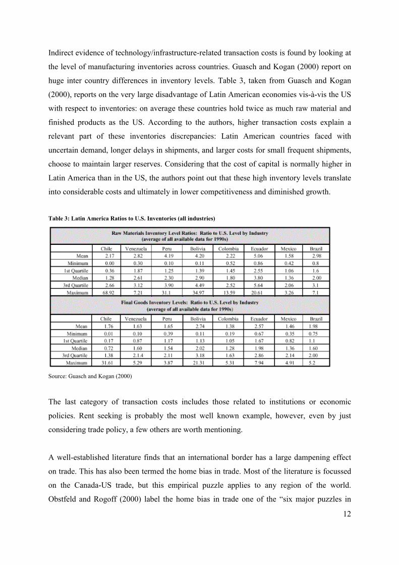
Indirect evidence of technology/infrastructure-related transaction costs is found by looking at

the level of manufacturing inventories across countries. Guasch and Kogan (2000) report on

huge inter country differences in inventory levels. Table 3, taken from Guasch and Kogan

(2000), reports on the very large disadvantage of Latin American economies vis-à-vis the US

with respect to inventories: on average these countries hold twice as much raw material and

finished products as the US. According to the authors, higher transaction costs explain a

relevant part of these inventories discrepancies: Latin American countries faced with

uncertain demand, longer delays in shipments, and larger costs for small frequent shipments,

choose to maintain larger reserves. Considering that the cost of capital is normally higher in

Latin America than in the US, the authors point out that these high inventory levels translate

into considerable costs and ultimately in lower competitiveness and diminished growth.

Table 3: Latin America Ratios to U.S. Inventories (all industries)

Source: Guasch and Kogan (2000)

The last category of transaction costs includes those related to institutions or economic

policies. Rent seeking is probably the most well known example, however, even by just

considering trade policy, a few others are worth mentioning.

A well-established literature finds that an international border has a large dampening effect

on trade. This has also been termed the home bias in trade. Most of the literature is focussed

on the Canada-US trade, but this empirical puzzle applies to any region of the world.

Obstfeld and Rogoff (2000) label the home bias in trade one of the “six major puzzles in

13

international macroeconomics”. With the existence of large home biases firmly established,

the search for explanations has begun. Evans (2000) finds little support for the hypothesis

that the home bias is not due to the border itself but instead to inherent differences in

domestic and foreign goods; Obstfeld and Rogoff (2000) argue that empirically reasonable

trade (i.e. transaction) costs can explain much of the home bias; and Anderson (2000) points

to information costs and imperfect contract enforcement as worthwhile avenues of inquiry.

Deep policy switches such as the creation of the common European market in 1992 have also

induced researchers to evaluate their economic impacts. A large collection of studies known

as the "Costs of Non-Europe", supported by the European Commission, mainly consists of

detailed estimations of the costs of the borders in Europe. The most cited reference is the

Checchini report that finds that these costs are considerable up to a small percentage of the

European GDP. Harrison, Rutherford and Tarr (1996) explicitly model these costs in a

general equilibrium framework and reach similar conclusions.

Another more recent example of trade-policy related transaction costs is found in Hertel,

Walmsley and Itakura (2001). The particular trade liberalization policy evaluated in their

study includes a series of measures intended to lower non-tariff trade costs between Japan

and Singapore. In fact, by imposing the adoption of computerized procedures, an explicit

objective of this policy was a reduction of the costs of customs clearance, a clear policy-

related transaction cost. For the case of the Japan-Singapore FTA, the effect of linking the

two customs’ systems is expected to generate additional reductions in effective prices

amounting to 0.065% in Japanese imports from Singapore and 0.013% in Singaporean

imports from Japan, and these cost saving refer solely to the cost of reduced paperwork,

storage and transit expenses. However, in addition to the direct cost savings, there are indirect

savings associated with the elimination of customs-related delays in merchandise flows

between these two countries. Hummels (2000) emphasizes that such time-savings can have a

profound effect on international trade by reducing both “spoilage” and inventory holding

costs. He argues that spoilage can occur for many types of reasons. The most obvious might

be agricultural and horticultural products that physically deteriorate with the passage of time.

However, products with information content (newspapers), as well as highly seasonable

(fashion) goods may also experience spoilage. Hummels points out that inventory costs

include not only the capital costs of the goods while they are in transit, but also the need to

14

hold larger inventories to accommodate variation in arrival time. He finds that the average

value of firms’ willingness to pay for one day saved in trade is estimated to be 0.5% ad

valorem (i.e., one-half percent of the value of the good itself). This value of time-savings

varies widely by product category, with the low values for bulk commodities and the highest

values for intermediate goods.

In summary, even if in identifying empirical estimates for transaction costs we have stretched

their definition to include quite different things, it seems clear that geographic characteristics,

poor transportation and communication infrastructure, and bad economic policies may

directly affect transaction costs, and that their presence can be documented in a variety of

ways.

For numerous examples of India specific transaction costs, refer to the appendix of the paper

and the references cited therein.

3. Transaction costs: some theory-consistent numerical simulations for India.

The following section considers two different ways of modelling transaction costs uses

several analytical structures to test how these modelling choices affect the evaluation of the

effects on aggregate income and relative poverty from reductions in transaction costs that

accompany conventional forms of liberalization. The ultimate objective is to draw

conclusions on the main channels of transmission from transaction costs reduction to income

determination (its level and distribution) and their likely empirical relevance in the real

world, and to do that different model versions are parameterised for India.

Transaction costs are modelled as either a mark up on the seller’s price or as icebergs melting

a la Samuelson. With the former approach, transaction margins generate income and they are

fully comparable to transportation margins, with the latter they simply produce costless

inefficiencies. These cost savings can affect transactions in goods market as well as in factor

markets.

The basic general equilibrium model used here represents a small price taker economy and it

is implemented here in three main versions: the first version is a standard Heckscher-Ohlin

15

international trade model with homogeneous goods, the second introduces intermediate

consumption, and the third considers a model with differentiated goods which generalizes the

Heckscher-Ohlin structure. A main contribution of the paper consists of pointing out how

differences in structural models matter for the estimation of the effects of transaction cost

reductions.

3.1 The Indian economy: stylised facts of a South Asian developing country

The crucial characteristics of our initial data for India are shown in Table 4, where it is

possible to observe some of the stylised facts of a typical developing country. The economy

has been aggregated into two sectors: an export oriented sector (Exportables) and an import

competing one (Importables). The first two rows in the table show the relative size of the two

sectors and their trade intensity (measured as exports or imports over production) using 1999

data. As expected India is relatively abundant in unskilled labour, and its exportables sector

uses more intensively this factor of production. The initial wage gap, measured as the ratio of

skilled over unskilled labour average incomes, is quite high with more skilled workers

earning almost five times more than unskilled workers. Exportables and importables use a

similar share of intermediates in production and bear an almost identical transaction cost, as

shown by the ‘ad valorem’ estimate.

Table 4: Initial 1994 data –main characteristics

Exportables Importables Economy-wideProduction shares % 46 54Trade Intensity % 10 8Skill Abundance Unskill / Skill 7.4Skill Intensity Unskill / Skill 65.9 11.1Skill Wage gap 4.7Intermediates as % of Production 50.6 50.3

Transaction Costs sector allocation 45 55Transaction Costs ad valorem % 15.0 13.0

Ownership shares Skill labour Unskill labourRural Heads own: 21 79Urban Heads own: 59 41

Consumption Shares Skill Head Unskill HeadExportables 59 49Importables 41 51

Sectors

Source: 1994 SAM for India (Pradhan B., K, A. Sahoo, and M.R. Saluja (1999)) and authors calculations

Notice also that transaction margins (when modelled as mark-ups) generate income that is

allocated across sectors in the same way as total demand (45 percent goes to exportables and

16

55 to importables). This deserves some further comment: whenever transaction margins are

reduced, the price wedge between seller and buyer is narrowed, and the total revenues raised

fall; initially these revenues are used to buy exportables and importables in fixed shares and

these shares are chosen to reflect the structure of total demand so that they should be as

neutral as possible. With this assumption, a fall in revenues should not directly affect the

overall demand structure. Clearly, another way of thinking of the sectoral allocation of

transaction margin income is that transaction costs are produced using exportables and

importables as inputs. The current sectoral allocation may not reflect the real world

“production structure” of transaction costs nevertheless, without additional empirical

evidence, the current choice allows to by-pass the problem without introducing unjustifiable

biases.10

Additionally, Table 4 displays households’ shares of factor ownership and goods

consumption. Households have been grouped into rural and urban and the factors ownership

structure shows that rural household are receiving a very large share of their income from

unskilled labour. Overall consumption shares do not differ greatly across households.

Most of the estimates shown in the table are direct calculations from India’s national accounts

and input-output tables, however transaction costs have been estimated using raw data on

geographic distances and inputs of transport/communication/distribution services.

In summary – in this set-up given similar sectoral ad valorem transaction margins, their

neutral revenue allocation and the across household similar consumption pattern – a reduction

in goods markets’ transaction costs affects households’ poverty and income mainly through

changes in factor rewards.

10 In fact one can think of two alternatives to this assumption: in the first, if it were known that producers of

transaction services are include exclusively in the importables sector, then transaction cost revenues could beentirely allocated to buy output from the importables sector. Alternatively, it may be possible to estimate atransaction cost production function that uses a mix of primary factors. In this case producers of transactionservices would minimize their cost of production subject to a budget constraint that equals transaction costsrevenues.

17

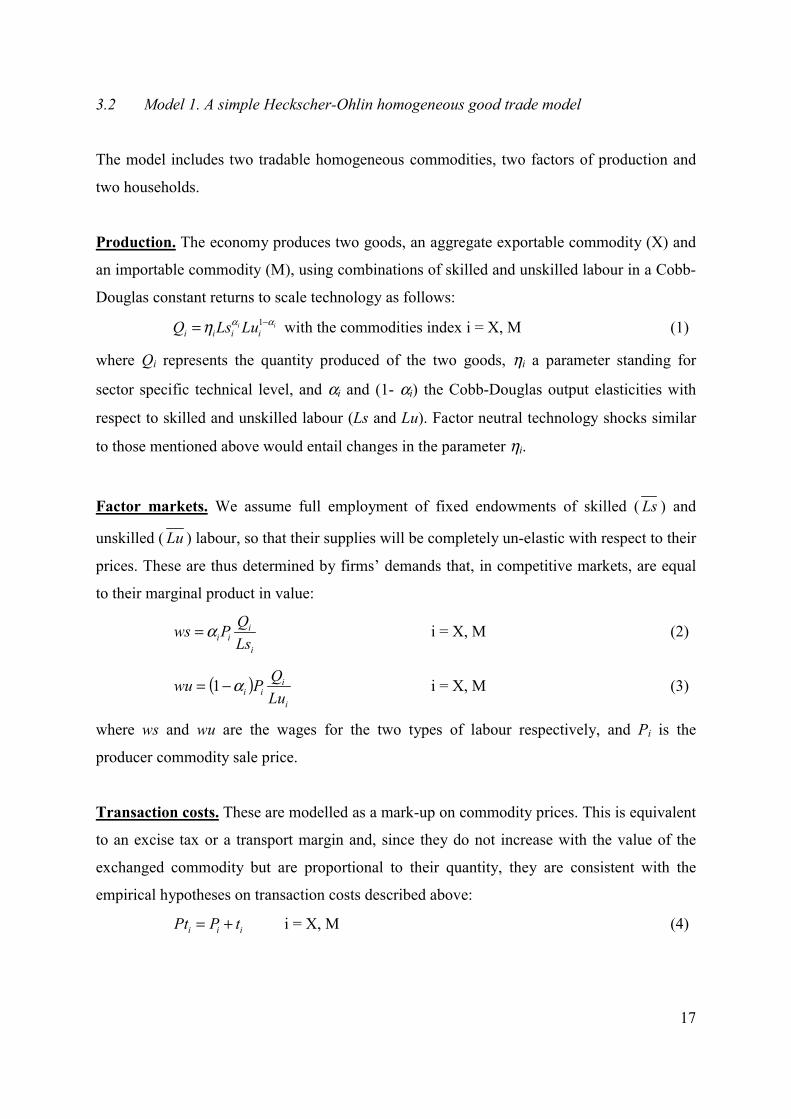
3.2 Model 1. A simple Heckscher-Ohlin homogeneous good trade model

The model includes two tradable homogeneous commodities, two factors of production and

two households.

Production. The economy produces two goods, an aggregate exportable commodity (X) and

an importable commodity (M), using combinations of skilled and unskilled labour in a Cobb-

Douglas constant returns to scale technology as follows:ii

iiii LuLsQ ααη −= 1 with the commodities index i = X, M (1)

where Qi represents the quantity produced of the two goods, ηi a parameter standing for

sector specific technical level, and αi and (1- αi) the Cobb-Douglas output elasticities with

respect to skilled and unskilled labour (Ls and Lu). Factor neutral technology shocks similar

to those mentioned above would entail changes in the parameter ηi.

Factor markets. We assume full employment of fixed endowments of skilled ( Ls ) and

unskilled ( Lu ) labour, so that their supplies will be completely un-elastic with respect to their

prices. These are thus determined by firms’ demands that, in competitive markets, are equal

to their marginal product in value:

i

iii Ls

QPws α= i = X, M (2)

( )i

iii Lu

QPwu α−= 1 i = X, M (3)

where ws and wu are the wages for the two types of labour respectively, and Pi is the

producer commodity sale price.

Transaction costs. These are modelled as a mark-up on commodity prices. This is equivalent

to an excise tax or a transport margin and, since they do not increase with the value of the

exchanged commodity but are proportional to their quantity, they are consistent with the

empirical hypotheses on transaction costs described above:

iii tPPt += i = X, M (4)

18

revenues generated by the wedge ti between the seller and buyer’s price are equal to ∑i

iiQt ,

and are used to buy transaction services from both sectors of the economy according to the

fixed structure described above.

Consumption. The model includes two households, a skilled headed (HHs) and an unskilled

headed (HHu) household, that receive income from selling factor services and demand

commodities via an optimisation of a Cobb-Douglas utility function. Households are thus

differentiated by their consumption patterns and according to their ownership shares, with the

skilled-headed household representing loosely the rich household. Derived consumption

demands are as follows:

i

HiHiH PtY

Qd β= with the household index H = hs, hu and i = X, M (5)

where Qd represents the household-specific quantity demanded, β a utility share parameter,

and Y the household’s income.

Trade and equilibrium conditions. Imports, exports and domestically produced goods are

homogeneous, so that trade, in any of the two goods, can only be one-way (either import or

export) and it originates only when domestic demand and supply differ. In equilibrium, trade

balance as shown below will hold:

0=∑i

iiTPw i = X, M (6)

Producers’ prices are equal to the world prices given the small country assumption, and

export or import flows quantities will be derived from the equality of supply and demand

where the latter includes final consumption as well as transaction services demands:

ii PwP = i = X, M (7)

iiH

iHii XQtQdMQ ++=+ ∑ i = X, M (8)

Factors’ market-clearing conditions simply state that the sums of factors demands must equal

the fixed factors’ endowments.

LLi

i =∑ and KKi

i =∑ i = X, M (9)

19

In this simple model the poverty measure is a relative poverty index equal to the ratio of

skilled to unskilled labour rewards. Given fixed factors ownership shares for the rural and

urban households and a poverty line, it would not be difficult to calculate absolute

households’ poverty measures. The advantage of considering household-specific absolute

poverty indices is that we would be able not only to trace the effects of changes in transaction

costs on the supply/income generation side, but also on the demand/income use side.

3.3 Model 2. A simple Heckscher-Ohlin homogeneous good trade model with

intermediate goods

This model introduces a simple variation in the previous one: the use of intermediate goods in

the production process. Intermediates are employed in fixed proportion to production with a

standard Leontief structure, so that equations (7) and (8) now become:

( ) jii

iiii atcPwPwP ∑ +−= i = X, M (7b)

iii

jiiH

iHii XQtaQQdMQ +++=+ ∑∑ i = X, M (8b)

where aji are the Leontief intermediate shares; notice that Pi’s now become value added

prices and these are equal to world prices minus the cost of intermediates which are valued at

world prices plus transaction cost mark-ups.

3.4 Model 3. A heterogeneous good trade model

This third model introduces several variants to the ones described above. First of all

transaction costs are modelled as iceberg wedges, i.e. the quantities sold by suppliers reach

the purchasers with a certain fractional loss (some quantity of the commodity melts away). In

this way transaction costs do not generate any income (or revenue) and they are in fact

denominated in the same units of measurement (i.e. real value or quantity) of the good

exchanged. In simplified terms the equilibrium quantity in a specific market would be:

iDi

Si tcQQ = (9)

where tci is a number greater than 1 representing the “melting” due to transactions costs.

20

In addition imports and domestically produced goods are imperfect substitutes in

consumption. Of the domestically produced goods one is not traded and only consumed at

home and the other is either exported or consumed. These changes alter the fixed world price

structure of the homogeneous goods model and allow for the price of the domestically good,

which is imperfectly substitutable with the imported one, to differ from the world price. This

type of model has been extensively used in the literature and its properties are well known.11

In this model there are 3 goods which enter the consumer utility function, an import good M,

a domestic non traded good D, and an export good X. Domestic production occurs only for D

and M with a CES technology that includes only skilled and unskilled inputs (the CES

function represents another difference form the models shown above).

The production function is:

( ) ( )[ ] iiiiiiii LssLuuQ

ρρρ ββ1−− += i = M, D

Factor markets equations remain unaltered apart from the obvious changes due to the new

functional form. Prices for commodities M and X are fixed and endogenously determined for

the non-traded commodity D; in fact supply and demand equilibrium such as in equation (9)

determines the price of D.

3.5 Numerical results

These simple general equilibrium models can be used to conduct a basic experiment aimed at

investigating the analytics of the link between relative poverty and transaction cost and the

aggregate effects of a reduction of the latter; the following numerical results should not be

considered exact estimates, but just indications on the potential magnitude and sign of that

effects.

As already described in the introduction, for a large body of literature, both empirical and

theoretical, globalization/openness improves an economy’s performance beyond the near

disappearance of tariffs’ deadweight loss triangles. In this study, openness is supposed to

11 See de Melo and Robinson (1989) or more recently Bhattarai et al (1999).

21

bring innovations in the transaction technology and their adoption is modelled by a decrease

in transaction costs without any indirect effect on the productivity of primary factors.

A first set of experiments, by using the three models described above, considers exogenous

reductions of transaction costs affecting the goods markets and estimates their effects on real

income and on the wage gap. In terms of the model’s parameter, the experiments consist of a

shock that reduces ti in equation (4) or tci in equation (9). A second set of experiments

considers exogenous reductions of transaction costs in factor markets. A final experiment

reverses the logic of the first two sets of experiments by shocking the economy with the

observed changes in real income and the wage gap (and other exogenous variables such as

factor supplies, technological progress, and international terms of trade), and thus estimating

the change in transaction costs.

Table 5 shows the results for model 1 of experiment 1: “50% reduction of exogenous

transaction costs in goods markets for all goods and all agents.” Given the fixed world prices

and un-elastic supplies of labour, a reduction in transaction costs does not produce any

change neither in domestic producers’ prices nor in factor rewards so that incentives to alter

output levels do not arise and output of both sectors stays constant. Relative poverty, the ratio

of skilled over unskilled wage, does not change due to the fact that resources do not move

across sectors. In this model, consumption due to transaction costs revenues is substituted by

households’ consumption (or exports) that can increase without an accompanying increase in

domestic output.

Table 5: Basic experiment of reduction in transaction costs, percentage variations with respect to initial equilibrium –model 1

Percent variations % %Output of Exportables 0.0 Exportables demand by HHr 13.2Output of Importables 0.0 Importables demand by HHr 10.8Producer price of Exp.ble 0.0 Exportables demand by HHu 13.2Producer price of Imp.ble 0.0 Importables demand by HHu 10.8Exports (volume) 7.5 Tc demand of exportables -43.6Imports (Volume) -5.0 Tc demand of importables -44.8

Wage S 0.0 Real HHr income 11.7Wage U 0.0 Real HHu income 11.7Ratio Ws / Wu 0.0 Total Real Income 11.7

It should be emphasised that even with different initial transaction costs across sectors or with

a sector bias in reduction of transaction costs, these results would not qualitatively change:

output and factor rewards will be still unaltered.

22

An important result obtained with this very simple model is that large increases, of more than

10 per cent, are registered in real incomes. These are large numbers and their occurrence is

entirely due to the elimination of the deadweight rectangles of transaction costs (rather than

the elimination of triangles associated for example to tariff reductions).

The same experiment, reduction of 50% of transaction costs mark-ups, produces quite

different relative poverty results when intermediates are introduced in the production process

as in model 2. In this case the reduction of transaction costs changes the relative profitability

of the two sectors: the exportables sector, using a larger share of intermediates, enjoys larger

savings than the importables one. This translates into a larger increase of the value added

price of exportables, 6.3 percent in contrast with 5.9 percent for importables, and into a large

increase of exportables output (see Table 6). Exportables use intensively unskilled labour that

now enjoys an increase in its reward: the relative poverty index improves by about 1 percent.

Table 6 Basic experiment of reduction in transaction costs, percentage variations with respect to initial equilibrium –model 2

Percent variations % %Output of Exportables 0.9 Exportables demand by HHr 13.6Output of Importables -0.8 Importables demand by HHr 12.7Val.Added price of Exp.ble 6.3 Exportables demand by HHu 13.3Val. Added price of Imp.ble 5.9 Importables demand by HHu 12.3Exports -4.4 Tc demand of exportables -46.7Imports -10.7 Tc demand of importables -47.1

Wage S 5.6 Real HHr income 13.2Wage U 6.4 Real HHu income 12.9Ratio Ws / Wu -0.8 Total Real Income 13.1

How robust is the relative poverty result? It can be easily shown that it crucially depends on

the sectoral differences in the Leontief aij coefficients, which directly influence the size of the

savings due to the reduction in transaction costs. The same experiment performed on an

Indian economy where all sectors were assigned the same intermediates coefficients would

produce identical changes in both skilled and unskilled wages, even in the case of sectorally

unequal transaction costs mark-ups.

It should be stressed though that a reduction in transaction costs brings positive increases in

both labour types wages so that absolute levels of poverty (and welfare) should be reduced

(increased) with a reduction in transaction costs.

23

Given that model 3 introduces a third non-tradable sector, before commenting experiment

results, a new table with the salient characteristics of the Indian economy is shown below.

Table 7 displays the main changes that affect the structure of the initial Indian data for this

third model and it should be contrasted with Table 4 above. Salient features are the high skill

labour intensity in the production of domestic non-traded goods (this is derived mainly from

the production structure of non-tradable services that include a high percentage of white

collar workers of the government sector, a large employer in India), and the lower transaction

wedge experienced in exchanges in the same sector.

Table 7 Initial data –main characteristics with a non-tradable sector

Importables Exportables Domestic Economy-wideProduction shares % 47 53Trade Intensity % 100 24 0

Skill Abundance Unskill / Skill 7.4Skill Intensity Unskill / Skill 23.7 3.3Skill Wage gap 4.7

Transaction wedge (goods mkts) 1.15 1.15 1.13

Transaction wedge (factors mkts)Skilled workers 1.20 1.20 1.20Unskilled workers 1.20 1.20 1.20

Sectors

Results from the basic experiment performed with the third model are shown in Table 8. The

main novelty here is that a reduction in transaction cost seems to have a lower effect on

aggregate income. This qualitatively different outcome can be fully explained by the initial

sectoral difference in transaction wedges. In model 1, sectoral differences in transaction cost

mark-ups do not matter for relative poverty, but in this model they are crucial. Due to the fact

that domestic goods are not perfect substitutes with importables, a sectorally differential

transaction cost shock alters relative prices across these categories of commodities, and

triggers a series of additional effects on output levels, factors’ allocation and rewards. A

reduction of transaction costs lowers the wedge between demanded and supplied quantities of

each commodity. Given the small country assumption, prices of “M” and of “X” do not

change and, for these markets, the new equilibrium is reached via changes in export and

import flows. Conversely, commodity D’s price is endogenous and is reduced. In turn, a

falling price results into lower profitability for this sector and gives rise to resources

reallocation. Finally, a reduction in wages of skilled workers is due to the more intensive use

of this factor in the production of commodity D with respect to the other sectors.

24

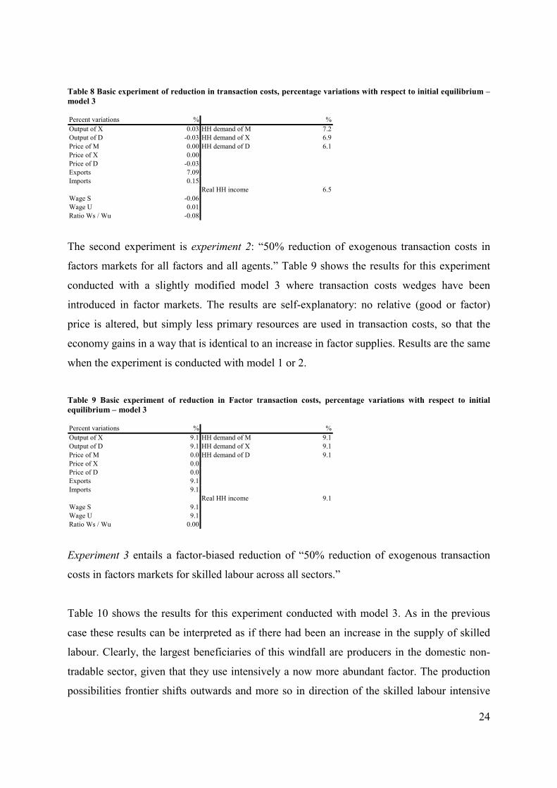
Table 8 Basic experiment of reduction in transaction costs, percentage variations with respect to initial equilibrium –model 3

Percent variations % %Output of X 0.03 HH demand of M 7.2Output of D -0.03 HH demand of X 6.9Price of M 0.00 HH demand of D 6.1Price of X 0.00Price of D -0.03Exports 7.09Imports 0.15

Real HH income 6.5Wage S -0.06Wage U 0.01Ratio Ws / Wu -0.08

The second experiment is experiment 2: “50% reduction of exogenous transaction costs in

factors markets for all factors and all agents.” Table 9 shows the results for this experiment

conducted with a slightly modified model 3 where transaction costs wedges have been

introduced in factor markets. The results are self-explanatory: no relative (good or factor)

price is altered, but simply less primary resources are used in transaction costs, so that the

economy gains in a way that is identical to an increase in factor supplies. Results are the same

when the experiment is conducted with model 1 or 2.

Table 9 Basic experiment of reduction in Factor transaction costs, percentage variations with respect to initialequilibrium – model 3

Percent variations % %Output of X 9.1 HH demand of M 9.1Output of D 9.1 HH demand of X 9.1Price of M 0.0 HH demand of D 9.1Price of X 0.0Price of D 0.0Exports 9.1Imports 9.1

Real HH income 9.1Wage S 9.1Wage U 9.1Ratio Ws / Wu 0.00

Experiment 3 entails a factor-biased reduction of “50% reduction of exogenous transaction

costs in factors markets for skilled labour across all sectors.”

Table 10 shows the results for this experiment conducted with model 3. As in the previous

case these results can be interpreted as if there had been an increase in the supply of skilled

labour. Clearly, the largest beneficiaries of this windfall are producers in the domestic non-

tradable sector, given that they use intensively a now more abundant factor. The production

possibilities frontier shifts outwards and more so in direction of the skilled labour intensive

25

product (“D”), and the relative (consumer) goods prices shifts in favour of this same product;

producers supply more D thanks to the lower costs of employing skilled labour. The skilled

wage premium is reduced and aggregate income rises (notice that skilled labour in volume is

about 12% of total employment).

Table 10: Reduction in Factor (skilled L) transaction costs, % variations with respect to initial equilibrium – model 3

Percent variations % %Output of X -0.7 HH demand of M -1.7Output of D 7.1 HH demand of X -0.4

HH demand of D 7.1Price of M 0.0 Consumer Price of M 0.0Price of X 0.0 Consumer Price of X 0.0Price of D -6.6 Consumer Price of D -6.6Exports -1.7Imports -1.7 Real HH income 3.2

Wage S -5.0Wage U 2.7Ratio Ws / Wu -7.5X's Lab Dem of S 5.0 X's Lab Dem of U -1.7D's Lab Dem of S 10.1 D's Lab Dem of U 3.1

The symmetric experiment of a biased reduction in unskilled labour transaction costs is

summarised in Table 11. It should be emphasised that, as in the previous case, the increased

supply effect (due to the reduction in transaction costs) dominates the wage-gap change: here,

more abundant unskilled workers gain more in absolute terms but less relative to the scarcer

skilled workers.

Table 11: Reduction in Factor (unskilled L) transaction costs, % variations with respect to initial equilibrium –model 3

Percent variations % %Output of X 9.8 HH demand of M 10.9Output of D 1.6 HH demand of X 9.4

HH demand of D 1.6Price of M 0.0 Consumer Price of M 0.0Price of X 0.0 Consumer Price of X 0.0Price of D 7.2 Consumer Price of D 7.2Exports 10.9Imports 10.9 Real HH income 5.7

Wage S 14.5Wage U 6.0Ratio Ws / Wu 7.9X's Lab Dem of S 4.0 X's Lab Dem of U 11.0D's Lab Dem of S -1.0 D's Lab Dem of U 5.7

Experiment 4 entails a: “50% reduction of tariffs with no change in transaction costs”.

Initially tariffs on importables are quite high at 46% and their reduction makes imports

26

cheaper relatively to domestically produced goods; this changes incentives for production and

triggers resource reallocations.

Results shown in Table 12 are completely in line with traditional modelling of trade

liberalization, in particular it should be noticed that real income effects are quite small (less

than 1 per cent), especially when compared with results obtained through a reduction in

transaction costs.

Table 12 Basic experiment of reduction in tariffs, percentage variations with respect to initial equilibrium – model 3

Percent variations % %Output of X 2.0 HH demand of M 18.4Output of D -1.8 HH demand of X -3.1

HH demand of D -1.8Price of M 0.0 Consumer Price of M -15.8Price of X 0.0 Consumer Price of X 0.0Price of D -2.2 Consumer Price of D -2.2Exports 18.4Imports 18.4 Real HH income 0.9

Wage S -4.3Wage U 0.9Ratio Ws / Wu -5.09

With the aim of describing the recent evolution of the Indian economy, all the shocks

previously examined are summarized in a final experiment. In this case, rather than assuming

exogenous changes in transaction costs and measuring their effects on the Indian economy,

the model “fits” the actual data and residually estimates transaction costs variations. More in

detail, the model is calibrated on an initial equilibrium for 1988 and, by changing exogenous

factors supplies, technological change, trade policy, terms of trade shocks, it is used to

estimate a new 1994 equilibrium. The model results, in terms of GDP growth and wage gap,

do not perfectly reproduce observed 1994 data and, at this stage, transaction costs are allowed

to vary so that the model can correctly reproduce observations. In this way, the model

provides an indirect estimate of the variation in transaction costs that ensures consistency

with observed data.

Table 13 below shows the recent evolution of the Indian economy since it implemented its

major structural reforms. The bottom panel shows a considerable spike (of almost two per

cent per annum) in the growth rate of the sub-continent. Results shown in the previous

experiment on trade liberalization clearly show that a standard model cannot account for this

27

sort of change in the growth rate: some additional structural change is taking place and need

to be explicitly introduced in the model.

Table 13 India – recent economic evolution

Variables \ Periods 1988 1994 1988/94 change

GDP constant 1988 price LCU (millions) 4,194,400 5,633,150 34.30

Wage Skilled 47.1 84.6 79.70Wage Unskilled 18.8 36.1 91.92Ratio (S / U) 2.5 2.3 -6.36

Labor Skilled (millions) 29 39 34.18Labor Unskilled (millions) 223 246 10.40

Tariff (average weighted in %) 87 46 -47.13

TFP index (economy wide) 100 115 15.00

1960-1987 1988-1999Average yearly GDP growth rate 3.88 5.69

Initially the model is used to re-produce the 1994 equilibrium; in particular, four main

exogenous changes are considered: a) change in tariff rates, b) terms of trade shock, c)

changes in factor supplies, d) change in TFP (applied with no sector biases); then these four

shocks are combined together.

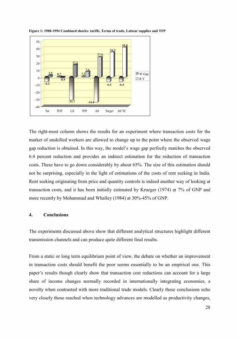
The wage gap and GDP variations resulting from this set of experiments are shown in Figure

1. Tariff reduction decreases the wage gap by inducing resource re-allocation consistent with

Indian comparative advantage and this has also a mild positive effect on real income; terms

of trade shocks (consisting in a 10% reduction of the price of Indian exportables) produce a

minor increase in the wage gap accompanied by a small real income reduction; changes in the

labour supply of skilled and unskilled workers has major effects for both the wage gap and

income, in particular skilled workers become relatively less scarce and their wage premium is

considerably reduced; finally, technological progress has strong positive effects on real

income and minor consequences for the wage gap. Combining all these shocks together

produces the results shown in the column “All”. This compares quite well with column

“Target”, which represents observed 1988-94 variations in the wage gap and real income,

although the “model” wage gap seems to decrease much more than the “real world” wage

gap, and, conversely, real incomes increase more in observed than model produced data.

28

Figure 1: 1988-1994 Combined shocks: tariffs, Terms of trade, Labour supplies and TFP

-6.2

2.5 0.7

-0.9

-31.7

17.2

1.17.4

-34.6

27.6

-6.4

34.3

-6.4

41.0

-40

-30

-20

-10

0

10

20

30

40

50

Tar TOT LS TFP All Target All TC

W GapR Y

The right-most column shows the results for an experiment where transaction costs for the

market of unskilled workers are allowed to change up to the point where the observed wage

gap reduction is obtained. In this way, the model’s wage gap perfectly matches the observed

6.4 percent reduction and provides an indirect estimation for the reduction of transaction

costs. These have to go down considerably by about 65%. The size of this estimation should

not be surprising, especially in the light of estimations of the costs of rent seeking in India.

Rent seeking originating from price and quantity controls is indeed another way of looking at

transaction costs, and it has been initially estimated by Krueger (1974) at 7% of GNP and

more recently by Mohammad and Whalley (1984) at 30%-45% of GNP.

4. Conclusions

The experiments discussed above show that different analytical structures highlight different

transmission channels and can produce quite different final results.

From a static or long term equilibrium point of view, the debate on whether an improvement

in transaction costs should benefit the poor seems essentially to be an empirical one. This

paper’s results though clearly show that transaction cost reductions can account for a large

share of income changes normally recorded in internationally integrating economies, a

novelty when contrasted with more traditional trade models. Clearly these conclusions echo

very closely those reached when technology advances are modelled as productivity changes,

29

and the transaction cost approach may indeed complement that of productivity. However,

unless technology is modelled endogenously, a daunting task especially when developing

countries are the object of study, a productivity shock represents a totally exogenous

windfall, whereas a reduction in transaction costs feeds back in the models used here in a

reduction of intermediation, and may be simpler to implement empirically. Notice also that,

in the models examined here, transaction costs affects only commodity exchanges, but it

should not be too difficult to introduce them also in factors markets. In this way it would then

be possible to simulate changes in education, training, health, or even migration, that

originate from lower transaction costs, even larger numbers may thus emerge.

5. References

Baldwin, Richard E. and Anthony J. Venables (1995). “Regional Economic Integration,” in

Gene Grossman and Kenneth Rogoff (eds.), Handbook of International Economics, Vol.

III , Elsevier, Amsterdam.

Bresnahan, T. and Manuel Tratjenberg (1995) General Purpose Technologies: ‘Engines of

Growth’ Journal of Econometrics 65: pp. 83-108.

Brown, Drusilla K. (1993). “The Impact of a North American Free Trade Area: Applied General

Equilibrium Models,” in Nora Lusting, Barry P. Bosworth, and Robert Z. Lawrence, (eds.)

Assessing the Impact, North American Free Trade, Washington, D.C.: The Brookings

Institution.

Burfisher, Mary E. and Elizabeth A. Jones, eds. (1998). Regional Trade Agreements and U.S.

Agriculture, Economic Research Service, AER No. 771. Washington, DC: U.S. Department

of Agriculture.

Coase R. (1937), “The Nature of the Firm”, Economica 4 (November), pp. 386-405.

Debreu, G. (1959), Theory of Value: An axiomatic analysis of economic equilibrium, Wiley,

New York

Elbadawi, Ibrahim, Taye Mengistae, and Albert Zeufack (2001) “Geography, Supplier Access,

Foreign Market Potential, and Manufacturing Exports in Africa: An Analysis of Firm Level

Data” World Bank Working Paper.

30

Foley D.K. (1970), “Economic Equilibrium with Costly Marketing” Journal of Economic

Theory, 2, pp. 276-291.

Francois, Joseph F. and Clinton R. Shiells (1994). “AGE Models of North American Free

Trade,” in Joseph F. Francois and Clinton R. Shiells, eds. Modeling Trade Policy, Applied

General Equilibrium Assessments of North American Free Trade, Cambridge:

Cambridge University Press.

Freund C. and Weinhold D. (2000), “On the effect of the Internet on international trade”. Board

of Governors of the Federal Reserve System – International Finance Discussion Papers

Number 693.

Goldberg V. (1985), “Production Functions, Transaction Costs and the New Institutionalism” in

Issues in Contemporary Microeconomics and Welfare, ed. G.R. Feiwel, Albany SUNY Press.

Hahn F.H. (1971), “Equilibrium with Transaction Costs” Econometrica, 2, pp. 276-291.

Helpman, Elhanan, ed. (1998) General Purpose Technologies and Economic Growth

Cambridge: MIT Press.

Henderson, Vernon, Zmarak Shalizi and Anthony Venables (2001) "Geography and

development", with, Journal of Economic Geography, 1, 81-106

Hertel, Thomas W., William M. Masters and Mark J.Gehlhar (1997). “Regionalism in World

Food Markets: Implications for Trade and Welfare,” Plenary paper for the XXIII

International Conference of Agricultural Economists, August 10-16, 1997, Sacramento,

California.

Jalan, J. and Ravallion, M. (1998) “Are there dynamic gains from a poor-area development

program?” Journal of Public Economics 67 pp. 65-85.

KPMG (2000), The Impact of the New Economy on Poor People and Developing Countries,

Draft Final Report to the UK Department for International Development, 7 July.

Kurz M. (1974), “Equilibrium with Transaction Cost and Money in a Single Market Exchange

Economy”, Journal of Economic Theory, 7, pp. 418-452.

Limao Nuno and Anthony Venables (2002), “Infrastructure, Geographical Disadvantage,

Transport Costs and Trade", with N. Limao, forthcoming in World Bank Economic

Review, World Bank, Washington.

31

Mohammad S and J. Whalley (1984), “Rent-seeking in India: Its costs and Policy Significance”

Kyklos, Vol 37- pp. 387-413.

Pradhan B., K, A. Sahoo, and M.R. Saluja (1999), “A Social Accounting Matrix for India, 1994-

95”, Special Article, Economic and Political Weekly, Mumbai, India.

Redding, Steve and Anthony Venables (2001) “Economic geography and international

inequality”, unpublished paper.

Samuelson P.A. (1954), “The transfer problem and transport costs, II: analysis of effects of trade

impediments”, The Economic Journal.

U.S. International Trade Commission (1992). Economy-Wide Modeling of the Economic

Implications of a FTA with Mexico and a NAFTA with Canada and Mexico, Publication

2516, May.

U.S. International Trade Commission (1998). The Economic Implications of Liberalizing APEC

Tariff and Non-tariff Barriers to Trade, Publication 3101, April.

Williamson O. (1975), Markets and Hierarchies, Free Press, New York.

Williamson O. (1985), The Economic Institutions of Capitalism, Free Press, New York.

Williamson O. (2000), “The New Institutional Economics: Taking Stock, Looking Ahead”,

Journal of Economic Literature Vol. XXXVIII (September) pp.595 –613.

32

APPENDIX: POLICY-RELATED TRANSACTION COSTS IN INDIA

This appendix should be considered as a partial updating of the 1984 Mohammad and

Whalley paper on rent seeking in India. In that paper, the authors estimate the cost of rent

seeking in India and quantify its magnitude at between 30% and 45% of GNP per year. They

also offer an extensive survey of the numerous economic policies that are likely to cause rent

seeking. It should be stressed that rent-seeking activity consists of using productive resources

in “processes generating outputs with no welfare valuation”, i.e. consists of wasting

resources, and, in this sense, rent seeking and iceberg-melting transaction costs are the same

phenomenon.

In what follows, a brief sketch of the recent (1985-2001) evolution of the Indian economic

policy controls is reported following the same headings of Mohammad and Whalley’s paper.12

1. External Sector Controls

1.1 Import Restrictions

1985-1990

The 1980s saw some attempts to simplify the import licensing system in order to provide

easier access to intermediate goods imports for domestic production by placing many such

items on the readily importable OGL (Open General License) list. To a lesser extent capital

goods imports were also eased through flexible operation of the discretionary regime in order

to encourage technological upgrading, particularly for export-oriented industries.

There was some replacement of quantitative import restrictions by tariffs, primarily in cases

where there was no competing domestic production.

The import tariff structure was somewhat simplified, however the average tariff rate went up.

12 The following text draws heavily on the three sources cited at the end of the appendix.

33

In October 1986, duty-free imports of capital goods were allowed in selected “thrust” export

industries.

In April 1988, access for exporters to imported capital goods was increased by widening the

list of those available on OGL and by making some capital goods available selectively to

exporters without going through “indigenous clearance”

1991-2001

In April 1992, a single negative list consisting of intermediate goods, a few capital goods and

most consumer goods replaced import licensing.

For most goods other than final consumer goods, the reform in the very first year largely

removed QRs (Quantitative Restrictions) on imports.

The QRs coverage for manufacturing (defined as the share of value added of the items

subject to import licensing to total value added) declined from 90 per cent in the pre-reform

period to 51 per cent in the 1994/95. It dropped to 29 per cent for capital goods and 35 per

cent for raw materials and intermediates; more de-licensing has followed. Certain petroleum

products are only major raw materials and intermediates whose import remains subject to

licensing, and practice even licenses are not quantitatively restrictive.

Liberalisation for consumer goods started in 1992 when a large exporters received Special

Import Licenses as an incentive, allowing them to import certain consumer goods specified

on a positive list. These licenses are freely tradable and their premium accrues to exporters.

The positive list has subsequently expanded. Baggage rules on consumer goods imports have

also been liberalised.

A phased reduction in tariffs thus became a central component of trade policy reform as tariff

rates came down in all the budgets presented from 1991 onwards, with the maximum tariff

decreased to 50 per cent in March 1995. Systematic reduction in the dispersion of tariff rates

produced eight rates of custom duty by April 1995 as opposed to 22 at the beginning of 1991.

In 1992, the Tax Reform Committee recommended that, by 1997/98, the tariff structure

should have custom duties of 20 per cent on capital goods, 25 to 30 per cent on intermediate

34

goods and 50 per cent on consumer goods. The government accepted the recommendations

with an open commitment to lower tariffs further.

Import duties on capital goods have dropped substantially. The composite rate on “project

imports” (imports of various capital goods needed to set up new projects), fell to 25 per cent

from 85 per cent. The duty on imports of machinery for electricity generation, petroleum

refining, and coal mining came down to 20 per cent; that for fertilisers dropped to zero. The

authorities left in place an earlier facility for duty-free imports of capital goods by firms

registered under the 100 per cent Export-Oriented Units (EOU) scheme and those in Export

Processing Zones (EPZs).

Intermediates goods such as metals and chemicals also obtained substantial tariff reductions.

Effective tariff protection for manufacturing has fallen from an estimated 164 per cent in

fiscal tear 1990/91 to abut 72 per cent in 1994/95.

The most recent 2001-02 official trade policy review (Exim policy) considers the following

points: a) QRs are totally dismantled; b) standing group to be set up for monitoring import of

300 sensitive items; c) import of new and second hand automobiles allowed, but subject to

conditions; d) import of agricultural products like wheat, rice, maize, other coarse cereals,

copra and coconut oil has been placed in the category of state trading; e) free imports of

second hand capital goods from up to 10 years old.

1.2 Foreign exchange rationing

1985-1990

Since Indian inflation rose faster than that of its trading partners, a devaluation of the nominal

effective exchange rate of about 45 per cent was required and achieved. This reflects a

considerable change in the official attitude toward exchange rate depreciation, however

stringent restrictions still apply to foreign exchange trades.

35

1991-2001

The rupee was devalued in July 1991 by 24 per cent. Exchange-rate policy went through a

series of further changes from 1991 to 1993. In March 1992 a dual exchange-rate system was

introduced. Under the new regime, exporters surrendered 40 per cent of their foreign

exchange earnings to the Reserve Bank of India at the official exchange rate, retaining the

remaining 60 per cent for sale in the free market thus created, which automatically restricted

import demand to the available foreign exchange.

In March 1993, the government moved to a unified floating exchange rate. The exchange rate

settled at around Rs 31=$1, between the old exchange rate of Rs 24=$1 and the free-market

rate of Rs 34=$1. Thus, the nominal exchange rate shifted by 57.5 percent, from Rs 20=$1 in

June 1991 before the devaluation to Rs 31.5=$1 in March 1993.

The rupee is now fully convertible for current-account transaction.

1.3 Export controls and export promotion

1985-1990

Export incentives were substantially increased. Cash assistance and duty drawbacks went up.

The value of the incentives net of taxes increased from 2.3 per cent of the value of exports in

1960/61 to 11.1 per cent in 1989/90.

There was a widening of the coverage of products available to exporters against import

replenishment and advance licenses. Very substantial income tax concessions were given to

business profits attributable to exports. The traditional export subsidies (cash assistance,

premium on import replenishment licenses, and duty drawbacks) increased from 9 to 13 per

cent of total export.

In 1985 budget, 50 per cent of business profits attributable to exports were made income tax

exempt: in the 1988 budget this concession was extended to 100 per cent of the export

profits.

The interest rate on export credit was reduced from 12 to 9 per cent.

36

1991-2001

Reduced exports subsidies. With the removal of quantitative restrictions and a shift to a new

competitive exchange rate, a large part of the export subsidy regime was dismantled.

Cash compensatory support ended very early when the rupee was devalued by 24 per cent in

July 1991. Subsequently the International Price Reimbursement Scheme (IPRS), which

refunded to the user the difference between the world and domestic prices of major inputs

such as steel and rubber, was abolished from 31 March, 1994.

The major still present export incentives include duty drawback and the advance licensing

scheme to large exporters to import the needed inputs duty free. The EPZs and the scheme of

EOUs also continue. The Exim Policy of April 1995 has taken several steps of enhance

export incentives, e.g. provision for duty-free importation of capital goods and extension of

the EPCG scheme to the services sector; improvement in the Advance Licensing Scheme; an

introduction of a green channel facility for customs clearance by certain categories of

exporters.

2. Capital Markets controls

2.1 Industrial licensing

1985-1990

There was some dilution of external requirements as regards entry and expansion of capacity.

The list of industries open to large firms was extended, and the licensing procedure has been

simplified.

1991-2001

Restrictions on the operation of large industrial houses have been removed. Licensing

requirements for investment have been abolished for all except a few strategic and defence

industries. Many areas earlier reserved for the public sector are now open to private

entrepreneurs.

37

These measures resulted into a strong injection of domestic competition and market

orientation in the manufacturing industry.

It should be noticed that considerable resistance to reforms arises from public-sector

infrastructure monopolies. Thus, even though doors have been opened for both foreign and

domestic private investment into these sectors, actual progress has been slow.

The Statement of Industrial Policy 1991 reduced the list reserved for the public sector from

17 to eight. By the end of 1994, the only areas in manufacturing which continued to be

reserved to public firms were those related to defence, strategic concerns, and petroleum.

Even here the government may invite the private sector to participate, as it has in the case of

oil exploration and refining.

2.2 Banks and insurance companies controls

1991-2001

India’s economic reforms have extended to both the banking system and the capital markets.

To reduce the former dominance of the financial sector by public-sector banks with little

commercial discretion in allocating their lending, banking sector reforms have included

substantial interest rate deregulation, more liberal licensing of private-sector bank, and more

latitude for expansion of the branch networks of foreign banks. The issue of privatisation of

the public-sector banks has not yet been addressed.

Capital-market reforms have sought to free capital market from detailed, direct government

controls, replacing them by a system of supervision to ensure better disclosure, greater

transparency and thus more investor protection. Efforts are being made to modernise the

stock exchanges and improve trading practices and settlement systems. A major current

initiative is the introduction of legislation to establish a Central Depository System, which

would expedite settlement.

There have been no reforms in the insurance sector; an expert committee has recommended

opening it to private investment, including foreign investment, but no decision has yet been

taken.

38

2.3 Controls on foreign private investment

1985-1990

In the second half of the 1980s, government began to seek foreign investment in industries

deemed to be of the national importance.

1991-2001

Reforms in policy towards foreign investment began with a radically new approach to

Foreign Direct Investment (FDI) in the first year of the reforms. The new regime permits FDI

in virtually every sector of the economy. Foreign-equity proposals need not be accompanied

by technology transfers as required earlier. Royalty payments have been considerably

liberalised. In industries reserved for the small-scale sector foreign equity can go up to 24 per

cent. Policy encourages foreign equity up to 100 per cent in export-oriented units, the power

sector, electronics and software technology parks. In other industries, foreign equity up to

100 per cent permitted discretionally. No restrictions hinder the use of foreign brand

names/trade marks for internal sale.

Although simplified, controls remain. A simple fast-track mechanism or “automatic

approval” from the Reserve Bank of India is available for projects of certain kinds, e.g. up to

51 per cent equity in high priority industries, up to 100 per cent equity in wholly export-

oriented units and all foreign-technology agreements, which meet certain economic

parameters. For all others, including cases involving foreign-equity participation of over 51

per cent, a high-level Foreign Investment Promotion Board (FIPB) reviews the applications.

About 20 per cent of the proposals have gone through the automatic route.

The Foreign Exchange Regulation Act (FERA) has undergone substantial amendment to

remove restrictive provisions on the operations of companies with foreign equity of 40 per

cent or more (commonly known as FERA companies). All companies incorporated in India

are now treated alike irrespective of the level of foreign equity. FERA companies can now

acquire and sell immoveable property. They can also borrow and accept deposits from the

public. Raising equity up to 51 per cent for these companies receives “automatic approval”, if

the investment are in any of 35 listed priority industries.

39

India has joined the Multilateral Investment Guarantee Agency (MIGA) for protecting

foreign investment against risks such as war, civil disturbance and expropriation.

The government specially encourages foreign investment in infrastructure, particularly the

power sector. Not only can foreign investor hold 100 per cent equity, but tax holidays are also

offered for five years for new power projects.

In the hydrocarbon sector, joint ventures are now permitted in both exploration and

development of oil fields and refineries. the telecommunication sector opened up with the

announcement in May 1994 of a new telecom policy providing for private investment in basic

telephone services as well as value-added services.

Air transport, until recently a public-sector monopoly, has opened to private sector, and new

entrants have begun operations. Private toll roads have also been commissioned.

In 1992 the government announced a new policy encouraging portfolio investment in Indian

industry. the Indian capital markets thus opened to foreign institutional investors such as

pension funds and broad-based mutual funds, subject to regulation by the Securities and

Exchange Board of India. Indian companies also gained access to capital markets abroad

through mechanisms such as Global Depository Receipts or Euro issues.

Substantially reduced restrictions on foreign investment produced an inflow of portfolio

investment that has grown from practically nil before 1991 to almost $3.5 billion per year

since fiscal year 1993/94, while direct investment grew to over $1.3 billion by 1994/95.

Outflows by residents are still forbidden or highly controlled. Inflows and outflows by non-

residents, have been partially deregulated. Foreign portfolio investment by residents is

forbidden.

40

2.4 Interest rates controls

1991-2001

Interest rate deregulation has been much faster since 1991. The process of liberalisation has

gone forward in commercial-bank deposit and loan rates. As recently as 1989/90, the interest

rate structure was still very complicated with 50 lending categories and a large number of

stipulated interest rates depending on loan size, usage and type of borrower. Starting in April

1992, the structure has become much freer and simpler. By the end of 1993, there were only

two restrictions on deposit rates: a fixed rate on savings deposits of 5 per cent and a

maximum rate of 10 per cent on term deposits (defined as deposits with maturities above one

and a half months). On the lending side, there was a minimum lending rate of 15 per cent for

loans above Rs 2 lakhs and a concessional rate of 12 per cent for very small loans. Since then,

there has been further deregulation. The lending rate for loans larger than Rs 2 lakhs has been

totally freed, though two concessional rates (13.5 per cent and 12 per cent) are now in place

for loans of smaller size. The cap on the deposit rate (now 12 per cent) applies only to

maturities of one and a half months to two years; the deposit rate for deposits longer than two

years is unrestricted.

2.5 Monopoly controls

1985-1990

The asset threshold above which firms are subject to monopoly regulation was raised.

Softening of restrictions on monopolies.

3. Controls in goods Markets

3.1 Price controls

1985-1990

Trough this form of intervention has been diluted, its scope nevertheless remains intensive.

The wholesale price index consists of a total of 360 commodities of which there are 55 major

items whose prices are fully administered, partially administered or subjected to different

forms of voluntary and other mechanisms of control. Fully administered items include

41

petroleum products, coal, electricity, fertilisers, iron and steel products, non-ferrous metals,

drugs and medicines, paper and newsprint.

3.2 Pricing and public enterprises

1991-2001

Budgetary support to public enterprises has been reduced. India’s infrastructure has not fared

well in the reform process. Market-orientation and domestic deregulation have focussed

largely on the manufacturing sector, while crucial areas of infrastructure like power

generation, telecommunications, roads and ports still function within a maze of regulation.

3.3 Controls on agriculture

1991-2001

The prices of all major agricultural products have been largely determined by the central

government’s control of foreign trade in them. The prices of cereals (rice, wheat, and coarse

grains) and cotton have been held below world prices in most years by controlling exports.

Sources:

Vijay J. and I.M.D. Little, India's Economic Reforms 1991-2001, Oxford University Press,

1997.

Vijay J and I.M.D. Little, India Macroeconomics and Political Economy 1964-1991, The

World Bank, Washington D.C., 1994.

Isher Judge Ahluwalia, Rakesh Mohan and Omkar Goswami, Policy Reform in India,

Development Centre Seminars, OECD 1996.