global value chain trade along the belt and road …...global value chain trade along the belt and...
TRANSCRIPT
Working Papers - Economics
Global Value Chain Trade along the Belt andRoad and Projects Allocation
Kaku Attah Damoah, Giorgia Giovannetti, Enrico Marvasi
Working Paper N. 07/2019
DISEI, Universita degli Studi di FirenzeVia delle Pandette 9, 50127 Firenze (Italia) www.disei.unifi.it
The findings, interpretations, and conclusions expressed in the working paper series are those of theauthors alone. They do not represent the view of Dipartimento di Scienze per l’Economia e l’Impresa

Global Value Chain Trade along the Belt and Road and Projects Allocation
Kaku Attah Damoah*†
Giorgia Giovannetti†‡
Enrico Marvasi†§
Abstract
We analyze the trade patterns among the countries involved in the Belt and Road Initiative (BRI) and investigate whether and to what extent they explain the allocation of investment projects regarding their number and value. Our findings indicate that investments tend to concentrate in countries already involved in global value chains (GVC) and especially favor suppliers of intermediate goods to China with similar sectoral specialization. At the same time, more developed countries closer to destination markets tend to attract fewer but larger investments. The BRI represents an opportunity for China to upgrade its exports and for the involved countries to join GVC productions.
Keywords: Belt and Road, China, global value chains, trade patterns.
JEL classification: F14, F15, F21.
* Corresponding author; email: [email protected] † Università di Firenze, via delle Panette 32, 50127 Firenze (Italy). ‡ European University Institute, Via dei Roccettini 9, 50014 San Domenico di Fiesole (Italy). § Politecnico di Milano, via Lambruschini 4/B, 20156 Milano (Italy). Acknowledgements: The authors wish to thank the participants of the 2018 Villa Mondragone Conference, the c.MET05 XV Workshop 2018, as well as participants of seminars in SACE (Rome) and Luiss (Rome) for their comments on previous versions of the paper. All errors remain ours.
Belt and Road
2
Table of contents
1 Introduction .............................................................................................................. 3
2 Corridors and investment projects ........................................................................... 4
2.1 Evidence for selected projects ............................................................................................ 7
3 Related literature ...................................................................................................... 8
4 Data sources ............................................................................................................. 11
5 Country characteristics and trade ............................................................................ 13
5.1 Income and projects ......................................................................................................... 13
5.2 Trade specialization and revealed comparative advantage ............................................ 15
5.3 Trade in intermediate goods ............................................................................................ 18
5.4 Trade of OBOR and projects recipient countries ............................................................ 19
5.5 The intermediate trade networks ..................................................................................... 21
5.6 Intra-industry trade ......................................................................................................... 25
5.7 Export and import sophistication ................................................................................... 26
6 Econometric analysis of project decisions .............................................................. 29
6.1 What characterizes OBOR countries .............................................................................. 29
6.2 The number of completed projects .................................................................................. 31
6.3 The value of completed projects ...................................................................................... 32
7 Conclusion ............................................................................................................... 33
References ...................................................................................................................... 35
Appendix.......................................................................................................................... 37
A1: Detailed projects information ................................................................................................ 37
A2: Detailed regressions .............................................................................................................. 39
A3: Indexes and measures ........................................................................................................... 42
Revealed comparative advantage indexes ............................................................................ 42
Intra-industry trade: GL index .............................................................................................. 43
Export and Import Sophistication indexes ............................................................................ 43
A4: Network centrality indicators ............................................................................................... 45
Belt and Road
3
1 Introduction
Officially announced by Xi Jinping in 2013, the Belt and Road Initiative (BRI), also called
One Belt One Road (OBOR), is China’s most ambitious geo-economic and foreign policy
initiative in decades and the first example of “transnational” industrial policy. The BRI
shows a commitment to easing bottlenecks to Eurasian trade by building networks of
connectivity across Central, Western and Southern Asia, reaching out to the Middle East,
Eastern and Northern Africa. The project combines a land-based Silk Road Economic
Belt and a sea-based 21-st Century Maritime Silk Road connecting China to Europe.
Infrastructure development is the most explicit and visible aspect of the project,
given that the BRI has mostly involved building roads, rails, and ports. However, through
infrastructure development, the BRI has the potential to enhance policy coordination,
trade facilitation, financial integration as well as capital and labour mobility. The project
is particularly relevant for China since it can also help to tackle industrial overcapacity at
home and acquire political influence abroad through investment. The BRI does not
attempt to unbundle production and consumption - the vision of the original Silk Road -
but rather to unbundle different segments of the production chain (or to reconfigure
them internationally in a way that may be beneficial to China and its partners). This is
going to affect the division of labor between countries therefore having potentially an
important impact on development. Furthermore, through infrastructure development,
the BRI can help participating countries to improve their trade logistics thereby
increasing their potential to join international production networks. Global (or regional)
value chains, in turn, can trigger development and growth prospects, especially for low
and middle-income countries.
Through the BRI, China is determined to strengthen its trade relationships with
neighboring countries by developing new export markets in Central, South and
Southeast Asian countries as well as secure suppliers for its manufacturing. By virtue of
BRI-related investments, existing value chains are likely to be reconfigured in the region.
Likewise, improving access to intermediate inputs would enable China to upgrade its
production.
In this paper, we concentrate on the trade-related aspects of the initiative. To the
best of our knowledge, we are the first to quantitatively assess a relation between OBOR
projects, trade and specialization.1 We construct a novel database of all completed
projects in countries along the corridors. We then assess the international trade motives
1 As the Belt and Road initiative is still in its initial phase, the research on the topic is scarce, especially quantitative studies. For a review see Section 3.

Belt and Road
4
behind the investments and explore which characteristics make countries more
attractive and suited as project recipients. Our research questions are: What trade
patterns characterize OBOR countries and project recipients? And what trade-related
characteristics make countries more likely to be actively involved in the initiative and to
reap the possible benefits? Specifically, we study whether OBOR investments, mostly
infrastructural, favor countries that are more involved in intermediate trade and/or trade
more intensely with China. We also examine whether sectoral specialization and the
trade patterns, including countries’ position in trade networks, play a role in the projects
allocations. Based on this evidence, we then investigate econometrically what trade-
related aspects are more likely to drive the investment project decisions.
In summary, we find that: i) investments seem to go towards large and relatively
poor countries, however, richer countries get fewer but larger investments; ii) project
recipients display relatively more diversified export structures than similar countries not
included in the BRI and their specialization tends to overlap with that of China; iii)
investments tend to favor countries that are more involved in GVC as suppliers of
intermediates to China; iv) China is clearly the center of the intermediate trade network
of OBOR countries, with some countries better positioned to represent crucial links to
other regions; v) countries more involved in intra-industry trade and with relatively
sophisticated export bundles are more likely to attract (larger) investments.
Our findings highlight that OBOR investments are closely related to trade patterns
and GVC considerations; therefore, not only they will contribute to strengthen the
regional GVC and related production networks, but also provide a reliable base of
suppliers to China, which in turn may able to upgrade its productions.
The rest of the paper is organized as follows. Section 2 describes the OBOR
corridors and projects. Section 3 introduces the related recent and growing literature on
the BRI initiative. Sections 4 describes the sources and construction of the dataset.
Section 5 provides descriptive analysis, while Section 0 presents an econometric analysis
of project decisions. Finally, Section 7 concludes.
2 Corridors and investment projects
Table 1 lists the main countries dividing them into regional areas (there is no official list).
More than sixty countries are somehow connected to the BRI. Their combined Gross
Domestic Product is $23 trillion (30% of world GDP), their population approximately
4.4 billion people (around 60% of the world population).

Belt and Road
5
Table 1 – Countries directly involved in the BRI.
Region Country East Asia China, Mongolia Southeast Asia Brunei, Cambodia, Indonesia, Laos, Malaysia, Myanmar, Philippines,
Singapore, Thailand, Timor-Leste, Vietnam Central Asia Kazakhstan, Kyrgyzstan, Tajikistan, Turkmenistan, Uzbekistan Middle East and North Africa
Bahrain, Egypt, Iran, Iraq, Israel, Jordan, Kuwait, Lebanon, Oman, Qatar, Saudi Arabia, Palestine, Syria, United Arab Emirates, Yemen
South Asia Afghanistan, Bangladesh, Bhutan, India, Maldives, Nepal, Pakistan, Sri
Lanka Europe Albania, Armenia, Azerbaijan, Belarus, Bosnia and Herzegovina, Bulgaria,
Croatia, Czech Republic, Estonia, Georgia, Hungary, Latvia, Lithuania, Macedonia, Moldova, Montenegro, Poland, Romania, Russia, Serbia, Slovakia, Slovenia, Turkey, Ukraine
Source: Industrial Cooperation between Countries along the Belt and Road, China International Trade
Institute. Note: The countries are grouped based on World Bank’s classification by region.
While there are different representations of the BRI, in line with Derudder et al.
(2016), we identify six different land corridors (Figure 1), encompassing the central cities
along the international routes and the economic industrial parks (as cooperation
platforms):
1. the China–Mongolia–Russia Corridor
2. the New Eurasian Land Bridge
3. the China–Central Asia–West Asia Corridor
4. the China–Indochina Peninsula Corridor
5. the China–Pakistan Corridor, and
6. the Bangladesh–China–India–Myanmar Corridor.

Belt and Road
6
Figure 1 – The six land corridors.
Source: Derudder at al. (2018).
China has put strong emphasis on the connectedness with the Central Asian and
South Asian countries, yet still little improvement in investment has been made, mainly
because of political and economic risk. However, in 2016, Chinese enterprises signed
7961 new contracts for OBOR-related projects, with initiatives spread unevenly across
countries. According to China’s Ministry of Commerce (Mofcomm), this amount
represents a 30.7% increase year on year, accounting for 51% of China’s total foreign
contract projects in the period (Mofcomm, 2017). The importance of the infrastructural
investments is also related to the fact that eight Central Asian countries are landlocked
(about one-fifth of the 44 landlocked countries in the world) and Uzbekistan is doubly-
landlocked countries (i.e. all its neighbors are also landlocked).
With regards to completed projects, a total of 329 major infrastructure projects,
including roads, railways, dry ports, and seaports, have been completed since the
inception of BRI.2 Roads account for 62% of projects, railways, dry ports, and seaports
for 13%, 10%, and 14% respectively. Also completed projects are not uniformly
2 The reported figure excludes infrastructure projects in other phases other than completed such as those planned, initiated, and/or under-construction.
Belt and Road
7
distributed across the recipient countries. The position of a country along a corridor is
likely to affect the number of completed projects. In 2018, Kazakhstan is the country with
most projects completed. Its 26 projects are mostly concentrated in roads (20), rail (4),
and dry port (2). Other countries with most projects completed are Cambodia (22),
Vietnam (21), Kyrgyzstan (21), and Pakistan (20). A list of all projects completed in each
country as at September 2018 is available in the Appendix A1.
2.1 Evidence for selected projects
In the last decades, production has been increasingly fragmented across firms and
countries at all income and development levels. Against this background, the degree of
competition along the Value Chains is also increasingly high for firms that have “to work
together” in a vertically integrated system of production. Producers in GVCs need to ship
parts, components, supplies, and finished goods quickly and cheaply both within the
region and to other regions. Most of the GVC production hubs in China (eastern coastal
cities) and Southeast Asia (e.g., Bangkok, Ho Chi Min City, Manila, and Singapore) have
access to ocean shipping and low transport costs. Central Asia does not have such access
and risks to be marginalized. Therefore, it is particularly relevant, especially for Central
Asia, where several countries are landlocked, to count on infrastructural investments.
The key GVC sectors are in multicomponent goods such as automobiles and
electronics. Automobile production is established in several Central Asian countries as
joint ventures with foreign producers. For instance, Toyota entered into a partnership
with Saryaka AvtoProm in 2014 to assemble a SUV in Kazakhstan. Less complex goods
are also produced through value chains. Textiles and garments are made in several
Central Asian countries. In some cases, they are produced largely from domestic inputs,
such as in Pakistan where cotton is grown and turned into fabric. In the Kyrgyz Republic,
for example, synthetic fabric is imported mainly from the PRC and made into clothing
that is exported and sold in Kazakhstan and the Russian Federation.
China needs to cultivate opportunities outside its borders. As an example, Wang
and Miao (2016) cite the Ruyi Group (Shandong), which has established weaving and
spinning plants in Pakistan to benefit from low labor costs and has also acquired stakes
in Australian and Japan textile manufacturers with the aim of setting up a truly
international value and marketing chain. Today, the group is involved in Japan,
Australia, New Zealand, India, and even the United Kingdom, Germany, and Italy.
Like Pakistan, Sri Lanka’s manufacturing sector is weak and has not been
integrated into the GVCs. Most Sri Lanka’s exports to China are resources, raw materials
and low-end manufactured products. The deep GVC integration of China’s
Belt and Road
8
manufacturing sector places it able to help with Sri Lanka’s GVCs participation through
manufacturing integration of the two countries (Kelegama, 2014).
3 Related literature
The BRI is a relatively recent project, but its width and the magnitude of its possible
effects are increasingly stimulating the research interests of researchers and policy
makers. Yet the literature investigating the economic aspects of the initiative is still in its
initial phase and quantitative studies are scarce. Most of the papers related to our work
have been circulating in the last couple of years, some of the earliest papers dating back
to just 2015, i.e. two years after the BRI was launched.
Some studies take a country perspective. For instance, Nataraj and Sekhani (2015)
and Banerjee (2016) argue that India, despite some distrust towards the initiative, should
welcome the projects as it is likely to gain from trade and from infrastructure building,
while an ineffective involvement may lead to some isolation risks. Adopting a broader
point of view, Cheng (2016), recognizing the complexity of the initiative and its strategic
importance, questions its real objectives. According to Huang (2016), the BRI was
promoted as an attempt to sustain China’s economic growth and transition towards a
more balanced development pattern, while also enhancing the country’s role in the
international setting.
Amighini (2017) includes several contributions with different perspectives on the
BRI, including an assessment on the new geography of trade and some policy
recommendations for the EU. The authors acknowledge that the initiative is likely to
transform the network of international trade routes reducing the dominance of maritime
connections in favor of the land corridors. This will in turn imply a deeper involvement
of some countries that will bring about implications also for the geopolitical relations
within the region. However, a key challenge for low and middle-income countries regards
their readiness to enter the international production networks. Some of these difficulties
can be overcome with a deeper integration of GVCs and domestic economic policies.
A two-part study by the Austrian Central Bank takes a project-oriented view of the
BRI, focusing on its implications for Europe. The first part of the study (Barisitz &
Radzyner, 2017a) reviews the initiative, its main institution and the details of some of
the main investment projects. Based on the evidence gathered, the authors stress how
maritime connectivity, while representing the dominant and cheaper mode is likely to
lose some ground to improved overland connectivity. The second part of the study
(Barisitz & Radzyner, 2017b) discusses the implications of the BRI for Europe, Southern
Eastern Europe in particular.
Belt and Road
9
Cai (2017) puts the BRI into perspective highlighting that China’s “comparative
advantages in manufacturing, such as low labor costs, have begun to disappear. For this
reason, the Chinese leadership wants to capture the higher end of the global value chain.
To do this, China will need to upgrade its industry.” (p. 8) Also, in the words of Hu
Huaibang, Chairman of the China Development Bank: “On the one hand, we should
gradually migrate our low-end manufacturing to other countries and take pressure off
industries that suffer from an excess capacity problem. At the same time, we should
support competitive industries such as construction engineering, high-speed rail,
electricity generation, machinery building and telecommunications moving abroad.”3
Yet, this China-centric approach might create some frictions with other countries along
the road, as some of their sectors are directly competing with China. This aspect is clearly
of primary economic importance for China’s trade and development and, therefore, for
the entire investment strategy behind the projects. Hence, in our work we explicitly take
it into consideration.
Bustos (2018) investigates the exposure of OBOR countries to trade shocks
originating from China. The author considers demand and competition shocks, the
former referring to China as an importer and the latter to China as an exporter. In the
last two decades, OBOR countries have been, on aggregate, a main destination of China’s
exports, but not a main source of China’s imports. The pattern seems to be gradually
changing, with some countries having increased their exports towards China.
Econometric results show that exports of OBOR countries were significantly impacted
by China’s demand shocks, while competition shocks became somewhat more important
in the last decade. The exposure to competition shocks is clearly related to trade
similarity and specialization overlap with China, however, we also argue that there is a
positive effect to consider as some degree of similarity can boost intra-industry trade and
within-sector specialization related to global value chains productions.
Derudder et al. (2018) explicitly take a network analysis approach and investigate
the hypothesis that a country’s position in the network of connections (road, rail, air, and
information technology) between OBOR countries matters for the possible gains from
the initiative. They conclude that prioritizing the weak links of the network is likely to
provide the largest benefits not only for the countries directly involved, but for the entire
network as well.
3 Hu Huaibang, “以开发性金融服务‘一带一路’战略 (Using Development Finance to Service the One Belt and One Road Strategy)”, China Banking Industry Magazine, 13 January 2016, http://www.cdb.com.cn/rdzt/gjyw_1/201601/t20160118_2187.html. Also cited in Cai (2017).

Belt and Road
10
Villafuerte et al. (2016) investigate the economic impacts of the BRI using the
GTAP model finding that there are possible benefits to trade and growth of both OBOR
and non-OBOR countries, with some heterogeneity between countries. More recently,
Enderwick (2018) offers an early stage assessment and discussion of the economic
impact of the BRI, also considering it in a historical perspective. Overall, the possible
benefits are heterogeneous, with some poorer countries benefiting greatly and China
being the major beneficiary.
Johns, Clarke, Kerswell, & McLinden, 2018 review the main trade facilitation
performance indicators (e.g. the logistics performance index, LPI) and discuss the
challenges of each of the six corridors. They show that OBOR countries tend to perform
poorly and proceed to identify the main priorities and recommendations, generally
calling for increased cross-country coordination and transparency measures to be
implemented on a corridor-by-corridor basis.
Two recent Eurasian Development Bank Reports study the BRI transport
corridors. Vinokurov Lobyrev, Tikhomirov and Tsukarev (2018) give a quantitative
assessment of the freight traffic along the corridors, concluding that there is little
uncertainty about the fast growth of container traffic in the next few years. In the second
report the same authors (Lobyrev, Tikhomirov, Tsukarev and Vinokurov, 2018) describe
the physical and regulatory barriers to freight traffic growth in the long run and the
investments that could foster it. Among the physical barriers, the relatively inadequate
transport and processing capacity of Polish railways is worth mentioning as Poland is the
main terrestrial gateway to the EU. The necessary improvements require sensible
investments in the area. Ghossein, Hoekman, & Shingal (2018), using the same data
source that we exploit in this paper (CSIS), describe procurement of BRI projects and
discuss possible improvements in procurement practices.
One of the main direct effects of the BRI is the reduction in trade and transport
costs, especially for the land routes. As stressed by (Amighini, 2017), “As there is no
comprehensive information available on the improvements to infrastructure or the
construction of new infrastructure, it is difficult to estimate how much transportation
costs will be reduced.” (Amighini, 2017 p. 135)
Quantification of the likely reduction in transportation costs is, in fact, one of the
first subjects on which the most recent studies have tried to shed light. Garcia-Herrero &
Xu (2017) provide one of the first estimates of the trade creation effects due to cheaper
transportation. Specifically, their econometric estimates indicate that the elasticity of
trade to transportation costs is 0.2 for railway, 0.55 for air and 0.11 for maritime. The
scenario-based simulations show that EU countries, especially landlocked, are likely to
Belt and Road
11
benefit. Results provided by Lu et al. (2018), based on a gravity model of trade, point to
a similar conclusion. Ramasamy, Yeung, Utoktham, & Duval (2017) investigate
econometrically the trade effects of improvements in both hard (i.e. physical) and soft
(i.e. administrative and ICT) connectivity, showing how expected gains vary from
corridor to corridor.
Focusing on production networks, Boffa (2018) studies the production and trade
linkages. Exploiting both custom trade data and input-output tables (TiVA, which
includes 28 OBOR countries), the paper gives an in-depth description of the trade
patterns and shows how regional trade integration between OBOR countries has
increased, mostly thanks to trade in intermediate goods and global value chains. The
paper also provides econometric estimates of the impact of trade costs on value-added
trade: a decrease in trade costs increases gross and value-added trade between OBOR
countries by 1.3-1.7%. Chen & Lin (2018) focus on foreign direct investments along the
BRI, shoving how improvements in transportation costs can have a positive impact also
on investments. The authors highlight that also in the case of FDI, the effects vary by
transportation mode.
Furthermore, there is a complementarity effects since OBOR infrastructural
projects seem to foster further subsequent Chinese FDI; a finding that is in line with Du
& Zhang (2018). Rather than focusing on trade effects or FDI, de Soryres et al. (2018)
explicitly study the impact of infrastructural project on shipment times and trade costs.
They build an original dataset which includes information on projects and their
geographical location and estimate that shipment times will decrease by 1.2-2.5%, which
in turn implies a reduction in trade costs by 1.1-2.2% at the world level; results indicate
even larger effects for OBOR countries, especially along the land corridors. Exploiting
the same data, Baniya, Rocha, & Ruta (2019) estimate a gravity model and comparative
advantage model to investigate the potential trade increases for participating countries.
4 Data sources
The data on infrastructural investments are taken from the Reconnecting Asia project of
the Center for Strategic and International Studies (CSIS). The CSIS Reconnecting Asia
project maps five infrastructural projects types – road, rail, seaports, intermodal
facilities, and powerplants – geographically spread in Eurasia countries from 2006 till
date. The compilation of the data by CSIS goes through three phases. First, primary
information on infrastructure is collected from open sources with key information such
as project type, cost, funders, commencement and projected completion dates. Primary
Belt and Road
12
sources of information include national agencies of host countries, regional development
banks, projects contracts as well as CSIS partners.
In the second phase, projects information is verified and de-conflicted by CSIS
research team to identify the most reliable and trustworthy information.4 Projects data
that passed the second stage screening process are then geotagged unto CSIS
Reconnecting Asia project website and uploaded with supportive information in the final
stage.5 The filter tool on the project website mentioned above enables one to search for
infrastructure projects by type, status (preparatory works, started, under construction,
completed, and cancelled), commencement and completion dates, as well as funders.
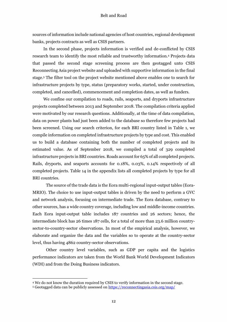
We confine our compilation to roads, rails, seaports, and dryports infrastructure
projects completed between 2013 and September 2018. The compilation criteria applied
were motivated by our research questions. Additionally, at the time of data compilation,
data on power plants had just been added to the database so therefore few projects had
been screened. Using our search criterion, for each BRI country listed in Table 1, we
compile information on completed infrastructure projects by type and cost. This enabled
us to build a database containing both the number of completed projects and its
estimated value. As of September 2018, we compiled a total of 329 completed
infrastructure projects in BRI countries. Roads account for 65% of all completed projects.
Rails, dryports, and seaports accounts for 0.18%, 0.03%, 0.14% respectively of all
completed projects. Table 14 in the appendix lists all completed projects by type for all
BRI countries.
The source of the trade data is the Eora multi-regional input-output tables (Eora-
MRIO). The choice to use input-output tables is driven by the need to perform a GVC
and network analysis, focusing on intermediate trade. The Eora database, contrary to
other sources, has a wide country coverage, including low and middle-income countries.
Each Eora input-output table includes 187 countries and 26 sectors; hence, the
intermediate block has 26 times 187 cells, for a total of more than 23.6 million country-
sector-to-country-sector observations. In most of the empirical analysis, however, we
elaborate and organize the data and the variables so to operate at the country-sector
level, thus having 4862 country-sector observations.
Other country level variables, such as GDP per capita and the logistics
performance indicators are taken from the World Bank World Development Indicators
(WDI) and from the Doing Business indicators.
4 We do not know the duration required by CSIS to verify information in the second stage. 5 Geotagged data can be publicly assessed on https://reconnectingasia.csis.org/map/

Belt and Road
13
5 Country characteristics and trade
Trade between China and its Central Asian partners increased substantially in the last
fifteen years. Back to 2000, the BRI countries only constitutes 13% of China’s exports
and 19% of China’s imports, but both shares have reached up to 27% and 23% by 2015.
The largest trading partners for China in the Belt and Road area are ASEAN countries
(12% of China’s total exports and 11.58% of total imports) with a relatively balanced trade
payment, partly because of their complementarity on value added chain. China’s second
largest trading partners within the BRI area are countries in the Middle East (from where
China mainly imports oils). South Asia is the third largest trading partner in the region
and has a very unbalanced bilateral trade as well as a complex product structure. Central
Asia, Central and Eastern European countries and Mongolia added up together account
for less than 3 percent of China’s external trade. Production and exports from Central
Asia currently are concentrated in oil, minerals, and agricultural products, although
there is considerable diversity among the countries and some countries are specialized
in manufacturing, typically textiles and machinery.
In what follows we focus our attention on OBOR projects and trade, especially of
intermediate goods, investigating several characteristics of the recipient countries.
Starting a project in one country rather than in another represents a clear signal of
preference or of higher expected return. The main recipients are likely to be the most
strategic countries for the overall BRI. To this end, it is convenient to separate countries
potentially involved in the BRI from those that received and completed projects. We thus
study the economic and trade characteristics of those countries vis-à-vis non-OBOR
countries and OBOR countries that did not get any project yet.
5.1 Income and projects
Let us consider GDP per capita. Averages of GDP per capita by groups are reported in
Table 2. Relative to the world average income per capita (about 14.7 thousand dollars),
OBOR countries are relatively poor (income per capita lower by about 4 thousand
dollars). This fact is of course mostly due to the geography of the BRI, which involves
many western and central Asian countries that are relatively poor and landlocked. OBOR
countries are in fact very heterogeneous. The income gap between countries with
completed projects and the other OBOR countries is even larger. The income of the
former is less than half that of the latter. In particular, income per capita of the project
recipients is about half the world average, while that of the other OBOR countries is 5
thousand dollars higher that the world average. Considering that many projects involve
roads, rails and ports, these numbers suggest that investments seem to go where the
Belt and Road
14
infrastructure is more lacking and perhaps the return on each dollar spent is likely to be
higher.
The opposite trend emerges when we consider population. OBOR countries are
larger than the world average, which is 40.6 million; however, this result is driven by
India: excluding India, OBOR countries are close to the world average population.
Among OBOR countries, the effect of India, which is among the project recipients, while
large, does not modify the evidence that projects tend to go towards large countries.
Again, the effect of country size may be related to gravity forces and to the fact that
projects may yield greater returns in larger markets.
Moreover, as projects tend to go towards relatively poor and populous countries,
one may wonder whether labor cost considerations may play a role in the decision of
where to invest.
Table 2 – Income and population of OBOR countries.
Per Capita GDP (2012) (US dollar)
Population (2012) (mln)
Population excl. India (2012) (mln)
OBOR 10627 50.2 29.9 of which
projects 7700 62.5 35.8 non-projects 19603 12.4 12.4
non-OBOR 16927 35.3 35.3
Total 14693 40.6 33.5 Note: Projects refers to OBOR countries with at least one completed infrastructure projects, while non-
projects refer to OBOR countries without any completed projects. Source: authors’ elaborations based on CSIS and WDI.
The above descriptive statistics show that there is a big difference between
countries that received investments and the others. However, investments may vary also
in number and in value; and one may wonder whether there is heterogeneity also within
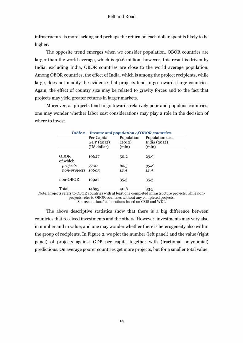
the group of recipients. In Figure 2, we plot the number (left panel) and the value (right
panel) of projects against GDP per capita together with (fractional polynomial)
predictions. On average poorer countries get more projects, but for a smaller total value.
Belt and Road
15
Figure 2 – Number and value of projects against GDP per capita.
Source: authors’ elaborations based on CSIS and WDI.
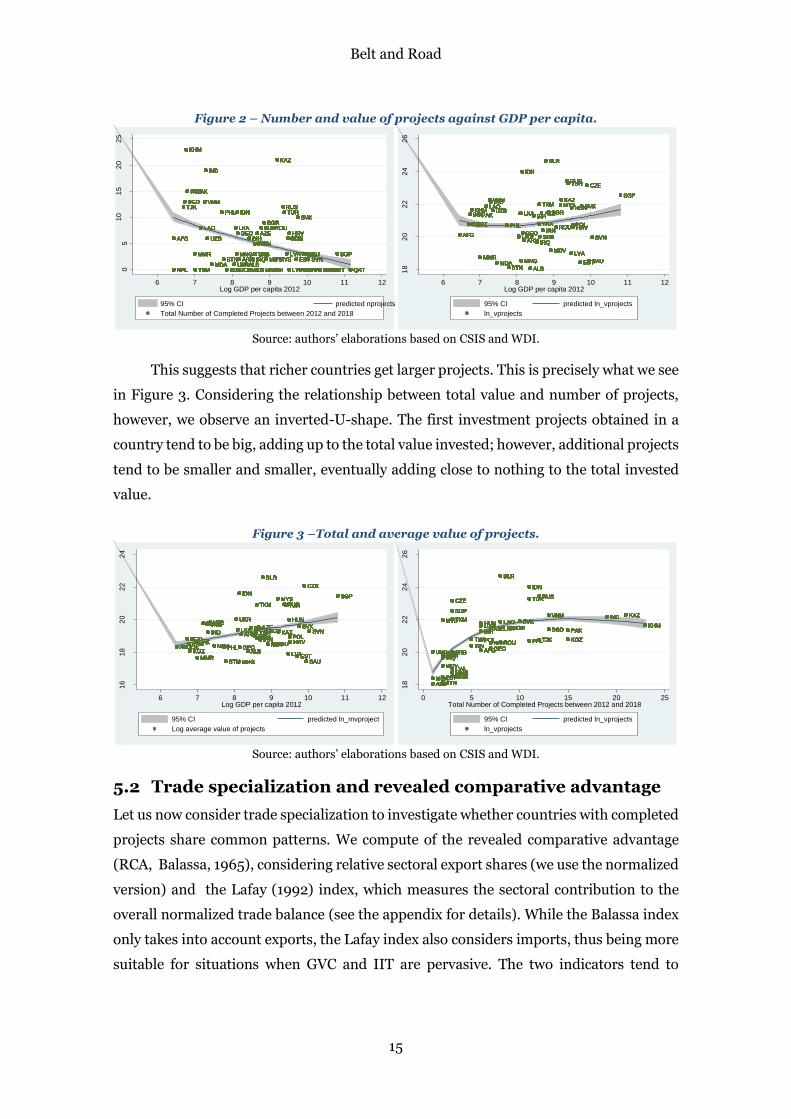
This suggests that richer countries get larger projects. This is precisely what we see
in Figure 3. Considering the relationship between total value and number of projects,
however, we observe an inverted-U-shape. The first investment projects obtained in a
country tend to be big, adding up to the total value invested; however, additional projects
tend to be smaller and smaller, eventually adding close to nothing to the total invested
value.
Figure 3 –Total and average value of projects.
Source: authors’ elaborations based on CSIS and WDI.
5.2 Trade specialization and revealed comparative advantage
Let us now consider trade specialization to investigate whether countries with completed
projects share common patterns. We compute of the revealed comparative advantage
(RCA, Balassa, 1965), considering relative sectoral export shares (we use the normalized
version) and the Lafay (1992) index, which measures the sectoral contribution to the
overall normalized trade balance (see the appendix for details). While the Balassa index
only takes into account exports, the Lafay index also considers imports, thus being more
suitable for situations when GVC and IIT are pervasive. The two indicators tend to
MMR
MNE
IRNUZB
BTN IRQ
AFG
ARM
NPLALB
MYS
BHR
SGP
MDALBN
AFG
UKR
TKM
KHM
LTUJOR
BTNMNG
JOR
IDN
UKRBTN
KAZ
SVNSVNLVA
MYSBTNMDA
TJK
AFG
BTN
KGZ
BLR
KAZ
LAO
KAZ
CZE
KHM
SRBMYS
QAT
KGZ
HUN
MKD
SAU
AFG
LAO
POL
PHL
MYS
BIH
KWT
LKA
JOR LTU
RUS
MDV
PAK
TJK
SVN
ARE
KAZ
SVK
TJK
YEM
SVN
LTU
MDV
PHL
MYS
QAT
PAK
PHL
MYS
THA
HRV
TUR
BHR BRNLBN BHR
GEOAFG
MNE
AZE
LBN
KAZ
YEM
GEO
MKD
BIH
MYS
PHL
LTU
BGR
LBN
HUN
VNM
UKR
AFG
VNM
MYS
AZE
THA
IRQ
EGY
MMR
IND
LVA
THA
YEM
SGP
MKD
LAO
NPLALB
MNGMMR SAU
ROU
LTU
BTN
BIH
PHLRUS
SVN
VNMVNM
SAUSVN
JOR QAT
HUN
EST
VNM
MKD
RUS
ARE
VNM
MDVSRB
VNMVNM
LAO
BIH
CZE SGP
OMN ISRYEM
IDN
TKMSVN
HRV
IND
ROU
SVNIRQ
AFG BIH
BGD
ALB
SGPMMR
LKA
SVKTUR
MYS
POL
YEM BRNALB
YEMMDA
YEM BRNALB
IRN
ALB
SVK
LBNYEM
HRV
ISR
SVKPHL
QAT
TKM
KWT
IRQSAU
QAT
POL
EGY MNE
SRB
BLR
QAT
CZE
LKA
UZB
LAO
EGY
IDN
EGY QAT
UZB
KAZ
MYS
TURSVK
MYS
UZB
KHM
IRQ
EGY
TUR
BTN
ARE
LAO
UZB
MDV
ISRKWTOMN KWTLBN
IND
MYS
RUS
LKAAZE
ROU
MMR
ALBNPL
BTN
KAZ
LKA
IRQUKR
LKA
IDN
LKALKALKA
IRQ
LKALKA
LTU ARE
TUR
BGR
MMREST
BGR
MNE
SVK
BTN
MNE
BGD
EGY
HUN
VNM
UKR
TKM
BRN
BGR
CZE
BIHAFG
ISR
PAK
MNG
AFG
JORMKD
ESTEST
ROU
TUR
MNEUKR
POL
UKRMDA
IND
UKRUKR
UZB
TKM
BHR
IDN
LAO
IRN
LVA SGPSGP
AREMKD
SRB LVA
PHL
KHM
PHL
THA
JOR
SVK
RUS
GEOBIH
MDA
IND
TJK
JOR
IND
SVN
IDN
SRBMYS
BGD
IND
BGR
AFG
BLRBLR
IDN
MMR
AFG
BLR
SVN
IND
NPL
BLR
AFG
BGR
NPL EGY
SVK
ESTALB
BLR
SVK
HRVUZB
EGY BRN
BLR
ARM
TUR
LVALVA
TJK
ARM
POLBIH
TKM
TUR
MNG
IRNPOL
THA
RUS
HRV
KWTBHRUKR
SAU
IDN
MDAAREAREMKD
POL
UKRARM
UKR
POL
EST
AFG
OMN
CZE
LBN
KGZ
LTU BHRJORJORUKR
HRV
KWT
TUR
KGZ
MMREST
SRB SGP
ARELBN
HUNHRV
LTUOMN
BLR
MNG
OMN
PHLSVK
MKD
LKA
AREMKD BHRMKD
UZBTHA
PHL
MKD
SGP
BRNISR
KHM
LBNMKD
THA
YEM LTU
LVA
BIH
EGY
PAK
ARE
LKA
IRQMMR
MKD
IDN
OMN
BGD
POL
SVN
KHM
BRN
TKM SGP
TUR
AZE
TKM
BLR
SGP
BHRNPL BHR ISR
KGZ
NPL
TKM
BGDBGD
TKMSRB
TJK
OMNBHR
AZE
TJKTJK RUS
TKM
TJKTJK
SVK
BHRLTU
TJK
EGY KWTLBN
GEOPOL
KGZ
JOR
SVNMMR
ISR
IDN
NPL
SVK
PAK
MMR
TUR
BGR
SVN
EGY
TUR
MMR
VNM
LBN
THATHABIHUZB
JOR
TKM
TURRUSTJK
BHR
GEOLKA
THAUZB
OMN
THA
TUR
THA
TUR
SAU
THA
IDN TUR
ROU
SGP
VNM
YEM
THA
YEM
ROU
MNG
THAAFG
BGD
YEM
ROUAZE
THA
SVN
LKALAOAZEAZE
KAZ
BGR
MKD
MMR LVA
ISR
IND
HRVHRV
CZE
AZEAZEBIH
HRV
MNG
HRV
PHL
LKA
ALBLTU
KAZ
ISR
VNM
MDVSRB
AZE
ARE
GEO
SRB
NPL
TUR
NPL
UZB
SRB
SVK
QAT
BGD
IND
TJK
IRQ
VNM
BRNYEM BHR
AZE
SAU
BGD
PHL
BRN
BLR
BHR BRN
SAU
HUNBIH
SGP
ALB
SAU
BRN
BGD
SAUSAUSAU
BGR
HRVPOL
KHM
BGR
IND
KWTMDA
IRQ
POLHRV
ESTARM MDV
LKA
BRN
TKM
THA
IRQCZE
ESTEST
IDN
CZE
MNE
RUS
OMN
AFG
PAK
OMN KWT
SVN
KHM
IRQ
KGZ
BTNSAU
OMNJOR
BGD
AFG
CZE
KWT
GEOUZB
ISR
CZE
KAZ
CZE
AFG
OMN
GEO
IDN
BIH
OMN
IRN
TJK
KAZ
SVK
RUSVNM
MDA
RUSRUS
ARM
KAZ
RUSRUS
SVK
RUSRUS
BGR
IND
VNM
MMR
PAK
KAZ
KHMKHM
KAZ
SVNSRB
POL
ROU
CZEBTN
OMN
ROU
BTN
KHMKHM
QATQAT
BGD
QAT
RUSRUS
MDV
QATMKDEGY LBN OMNUKR
BLR
SGP
ALBARM
SAU
MNE
IDN
EST
MNE
AFG
BLR
KHM
MDA
UZB
SRB
BGD
MDV
PHL
HRV
MYS
KAZ
JOR
POL
QAT
POL
PHL
ARE
SGPMMR
KWT
LVA
OMN
SRB LVA
AREUKR
PHL
MMR SAU
QAT
PHL
THA
PAK
ALB
IRNBIH
YEM
BGR
MDV
BLR
QAT
BTN
BRN
IND
SGP
IDN
KHM
BGD
LBNEGY
AFG
SRB
BGR
LVA
BIH
LTU
SRB
UKR
UZB
PAK
HRV
NPL
SVK
TJK
IRQ
PHL
ALBMKD
BGR
KGZ
SVK
KAZ
CZE
HUN
MNE
BGR
QAT
UZB
TKM
LAO
MDV
BIH
KHM
BTN
PHL
ARM
LAO
MNG
AZE
BHR
PAK
BLR
MKD
SGP
ARE
MNG
MNE
PAK
SVN
PAKPAKPAK
MNG TKM
THA
EST
IRN
ROU
SRBEST
ALB
UZB
IDN
AZE
QATBHR
TJK
BTN
JORJOR
ARM
MKD QAT
MNGSVN
SRB
PAK
MNE
AZE
BGD
ARM
LTU
ARM
HRV
OMN
SVKSVK
MNE
HRVAZE
SAUMNG
UKR
IND
IRN
EST
UZB
LAO
MYS
TUR
BIH
JOREGY MNEMKD ARE
TJKBGD
SVN
ROU
BRN
SVK
MDV
IND
SAU
KHM
SGP
TURTJK
PAK
IRN
EGYALB
TKM
HUN
BGD
UZB
MNE
BTNTKM
ARM
JOR
IRN
PAK
GEO
KGZ
CZE
THABIH
TKM
ISR
KAZ
BIHUZB
KGZ
AZE
IRN
MNG
GEO
BRN
SAU
LBNNPL
TKM
UKRJORYEM
BGR
IND
HRV
MKD
ARM
HRV
NPLNPLNPL
HUN
ARMMNG
BIH
NPL BRNNPL
BGR
RUS
POL
NPL
HRV
EST
BLR
SVK
MDAMNE BHRLTU
TKM
MDA
PHL
KGZ
ISRISR QATNPL ISROMN
GEOBIH
ISR
MMR
HRVLAO
TKM
ROU
MMR
MDA
SGP
YEM LBN ARE
CZE
GEO
IDN
ROU
UKRLTU
MDA
PHL
MDV
IND
MDA
SVK
PAK
SGPSVN
SRB
KWT
BTN
BIH
IRQ
JORMKDYEM
ESTCZE
MDV
MNEMNE
UZB
ARMUKR
CZE
EGY
AZEGEO
SGP
HUN
MNEMNE
IRN
MNE
AZE
OMN QATOMN BRNYEM
LVASVN
TJK
MNGMDV
SAUMDV
MNG
THA
ROU
POL
KAZ
UZB
BRN
IND
TKM
BGR
LTU
ARM
BLR
KWT
SAU
ISRMDAMDA
BLR
PHL
BTNMDA
RUS
MDA
KHM
ARM
LKA
VNM
ALBJOR
IRQ
IRN
MMR
POL
ROU
TJK
TKM
LAO
THA
TUR
KHM
MDA
GEOHUN
EST
HUN
QAT
BTN
PAK
MYSMNG
IRQMNG
IDN
VNM
KAZ
LTU
HUN
VNM
LVA
YEM
MYSSAU
KWT
KGZ
JOR
SGP
RUS
SRBMYS
BRN
MDV
LAO
ARE
KGZ
BHR
BGR
SGP
OMN QATLBNMKD
AZE
BGR
ARMTKM
ALBARM
OMN
HRVHUN
CZE
MKDEGY
THAUZBAFG
LVA
TJK
LKA
KWTEGY
UZB
EGY
MDVCZESRB
MDV
LTU
LVASVN
EGY BHR
MDV
EGY
MDV
HRV
MYS
SVK
KWT
BIHIRN
MDA
TUR
MYSARM
IRN
AZE
YEM
IND
BGR
MDA
BGD
LBNNPL
IDN
BRNLTU
ARM
BLR
ALB
MMR
TJK
ARM
AFG
MYSIRQLVA SGP
BRN
GEOGEO
UKRBTN
LVA
OMN
IDN
MMR
TUR
EGY
VNM
CZEMDV
NPL
IRQ ESTARM
BGD
GEO
EST
KWT
BTN ESTEST SVN
ROU
ESTMDA
HUN
PHLTJK
LKA
IRQ
QAT
KHM
IDN
YEM
UZB
LTU
HUNIRN
BRN
MNG
PAK
KAZ
LBN
MDV
IDN
LTU
IDN
BTN
ARE
MDV
QATISR
RUSVNM
HUN
MNE
BGR
LTUMKD
IND
SVN
GEO
MDA
THA
SVK
ARE
BGRROU
SAU
AFG
EST
SVK
GEO
JOR
BGR
UKR
SRB SAU
LAO LKA
ESTMMR
MYSSRB SGP
KHM
MKDEGY
BGD
BRNLBN
BLR
PHL
LBNLBN
MNG
PAK
BLR
LBN
ROU
NPL LBN
HUN
SRB
AZEBIH
QAT
KAZ
GEOUZB
ISR
ARM
BHR
POL
LVABTN
LVA
ARE
EST
IRN
LVAMNG
KHM
OMN
LAO ROU
POL
ISR
TUR
ISR
IRQ
LAOLAO ROUAZE
LAOLAO
MDA
LAO
NPL ISR
KGZ
EGY AREALB
KGZ
LAO
KGZKGZ
BRN
KGZKGZKGZ
BHRMDA
KGZ
KWT
BLR
SRB
KWT
LKA
KWT
RUS
ISR
BGR
SRB
IDN
SVNBTN
BGD
LVA
RUS
KAZ
CZE
POL
VNM
LKA
CZE
TJK
ISR
MNG SGP
VNM
BHR
VNMTJK
KHM
ROU
KAZ
TKM SAU
KGZ
ESTALBUKR
KAZ
TKM
ISR
KGZ
SRB
IRN
BTNMMR
RUS
EGYJOR
SAUSAU
TUR
MNE QAT
PAKPAK
JOR
SVK
IRQ
TUR
GEOGEOHUNBIH
ROUGEO
SGP
UKR
ROU
ALBBHR
AZE
NPL
BIHGEO
YEM
VNM
EGY
POL
BGD
ARM
KHM
ARE
MMR MNG
VNM
LAO
MNE
ROU
BHRLBN
TUR
GEO
MNE
POL
LVA
KWT
CZE
KWTYEM
HRV
ISRLTU
MMR
KGZ
KAZ
LAO
MYS
LTU
LKA
YEM
BGD
BTNALB
AFG
RUS
HUN
CZE
ROU
YEM BHR
MDV
POL
MYSIRQCZE
AFG
IRQ
KAZ
IRQIRQ
PHL
MKD
IRQ
THA
JOR
UZB
BGD
LKA
IRNPOL
KWT
IRN
LVA
KWT
LVA
PAK
IRNIRN
BRNALB
JOR
HUN
KHM
LVA
ALB
HRV
IRN
ROU
PHL
MYS
KGZ
TJK
OMNBHR KWTUKR
THA
BGD
IRN
NPL
MMR
IDN
KGZ
ISR
POL
IND
LVA
IRN
MNG
INDIND
BLR
IND
CZE
IND
ALBMYS
AFGAZE
ARM
AREKWT
PAK
LTUALBMDA
AFG
PAK
ARENPL LBN ARE
BLRBGR
BRN
HUN
BLR
HUNIRN
HUN
KHM
HUN
MNG
KHM
BLR
HUN
OMN
SVN
HRV
MDV
PHL
MDV
VNM
LKA
MNG
IND
AZE
BGD
MNE
LAO
LBN
GEO
IDN
LTU AREYEM
LAO
UKR
05
10
15
20
25
6 7 8 9 10 11 12Log GDP per capita 2012
95% CI predicted nprojects
Total Number of Completed Projects between 2012 and 2018
MMR
IRN
UZB
BTN
IRQ
AFGARM
ALB
MYS
SGP
MDA
AFG UKR
TKMKHM
BTN
MNG
IDN
UKR
BTN
KAZ
SVNSVN
LVA
MYS
BTNMDA
TJK
AFG
BTN
KGZ
BLR
KAZ
LAO
KAZ
CZE
KHM
SRB
MYS
KGZ
HUN
SAU
AFG
LAO
POLPHL
MYS
BIHLKA
RUS
MDV
PAK
TJK
SVN
KAZSVK
TJK
SVN
MDV
PHL
MYS
PAK
PHL
MYS
THAHRV
TUR
GEOAFG
AZE
KAZ
GEO
BIH
MYS
PHL
BGRHUN
VNM
UKRAFG
VNMMYS
AZE
THA
IRQ
MMR
IND
LVA
THA
SGP
LAO
ALB
MNGMMR
SAU
ROU
BTN
BIH
PHL
RUS
SVN
VNMVNM
SAU
SVN
HUN
EST
VNM
RUS
VNM
MDV
SRB
VNMVNM
LAO
BIH
CZE
SGP
IDN
TKM
SVN
HRV
IND
ROU
SVNIRQ
AFG
BIHBGD
ALB
SGP
MMR
LKA
SVK
TUR
MYS
POL
ALBMDA
ALB
IRN
ALB
SVK
HRV
SVK
PHL
TKM
IRQ
SAU
POL
SRB
BLR
CZE
LKAUZB
LAO
IDN
UZB
KAZMYS
TUR
SVKMYSUZBKHM
IRQ
TUR
BTN
LAOUZB
MDV
INDMYS
RUS
LKA AZE
ROU
MMR
ALBBTN
KAZ
LKA
IRQUKR
LKA
IDN
LKALKALKA
IRQ
LKALKA
TUR
BGR
MMREST
BGRSVK
BTN
BGDHUN
VNM
UKR
TKM
BGR
CZE
BIH
AFG
PAK
MNG
AFG
ESTEST
ROU
TUR
UKR
POL
UKR
MDA
IND
UKRUKR
UZBTKM
IDN
LAO
IRN
LVA
SGPSGP
SRB
LVA
PHL
KHM
PHL THA
SVK
RUS
GEO
BIH
MDA
IND
TJK
IND
SVN
IDN
SRB
MYS
BGD
IND
BGR
AFG
BLRBLR
IDN
MMR
AFG
BLR
SVN
IND
BLR
AFG
BGRSVK
ESTALB
BLR
SVK
HRV
UZB
BLR
ARM
TUR
LVALVA
TJK
ARM
POL
BIH
TKM
TUR
MNG
IRNPOLTHA
RUS
HRV
UKR
SAU
IDN
MDA
POL
UKRARM
UKR
POL
EST
AFG
CZE
KGZ
UKR
HRV
TUR
KGZ
MMREST
SRB
SGP
HUN
HRV
BLR
MNG
PHL
SVK
LKAUZB
THAPHL
SGP
KHM
THA
LVA
BIHPAK LKA
IRQ
MMR
IDN
BGD
POL
SVN
KHMTKM
SGP
TUR
AZE
TKM
BLR
SGP
KGZ
TKM
BGDBGD
TKM
SRB
TJK
AZE
TJKTJK
RUS
TKM
TJKTJK
SVK
TJK
GEO
POLKGZ
SVN
MMR
IDN
SVK
PAK
MMR
TUR
BGR
SVN
TUR
MMR
VNM
THATHA
BIHUZB
TKM
TURRUS
TJK
GEO
LKA
THA
UZB
THA
TUR
THA
TUR
SAU
THA
IDN
TUR
ROU
SGPVNM
THAROU
MNG
THA
AFG
BGD
ROU
AZE
THA
SVN
LKA
LAO
AZEAZE
KAZ
BGR
MMRLVA
IND
HRVHRV
CZE
AZEAZEBIH
HRV
MNG
HRVPHL
LKA
ALB
KAZVNM
MDV
SRB
AZE
GEOSRB
TUR
UZB
SRB
SVK
BGD
IND
TJK
IRQ
VNM
AZE
SAU
BGD
PHL
BLR
SAU
HUN
BIH
SGP
ALB
SAU
BGD
SAUSAUSAU
BGR
HRVPOL
KHM BGR
IND
MDA
IRQ
POLHRV
EST
ARM
MDV
LKA
TKM
THA
IRQ
CZE
ESTEST
IDN
CZERUS
AFG
PAK
SVN
KHM
IRQ
KGZ
BTN
SAU
BGD
AFG
CZE
GEO
UZB
CZE
KAZ
CZE
AFG GEO
IDN
BIH
IRNTJK
KAZSVK
RUS
VNM
MDA
RUSRUS
ARM
KAZ
RUSRUS
SVK
RUSRUS
BGR
INDVNM
MMR
PAK
KAZ
KHMKHM
KAZ
SVNSRB
POLROU
CZE
BTN
ROU
BTN
KHMKHMBGD
RUSRUS
MDV
UKR
BLR
SGP
ALB
ARM
SAU
IDN
EST
AFG
BLR
KHM
MDA
UZB
SRB
BGD
MDV
PHL HRV
MYSKAZ
POLPOLPHL
SGP
MMRLVA
SRB
LVA
UKR
PHL
MMRSAU
PHL THA
PAK
ALB
IRN
BIHBGR
MDV
BLR
BTN
INDSGP
IDN
KHMBGD
AFG SRB
BGR
LVA
BIH
SRBUKR
UZBPAK
HRV
SVK
TJK
IRQ
PHL
ALB
BGR
KGZ
SVKKAZ
CZE
HUNBGRUZB
TKMLAO
MDV
BIHKHM
BTN
PHL
ARM
LAO
MNG
AZEPAK
BLR
SGP
MNG
PAK
SVN
PAKPAKPAK
MNG
TKM
THA
EST
IRNROU
SRB
ESTALB
UZB
IDN
AZE
TJK
BTN
ARM
MNG
SVNSRB
PAK AZEBGD
ARMARM
HRV
SVKSVK
HRV
AZE
SAUMNG
UKR
IND
IRN
EST
UZBLAO MYS
TUR
BIH
TJK
BGD
SVN
ROU
SVK
MDV
IND
SAU
KHM
SGP
TUR
TJK
PAK
IRN
ALB
TKMHUN
BGDUZB
BTN
TKM
ARM
IRN
PAK
GEO
KGZ
CZE
THA
BIH
TKMKAZ
BIHUZB
KGZ
AZE
IRN
MNG
GEO
SAU
TKM
UKR
BGR
IND
HRV
ARM
HRV
HUN
ARM
MNG
BIHBGR
RUS
POLHRV
EST
BLR
SVK
MDA
TKM
MDA
PHLKGZ
GEO
BIH
MMR
HRV
LAO TKM
ROU
MMRMDA
SGP
CZE
GEO
IDN
ROU
UKR
MDA
PHL
MDV
IND
MDA
SVK
PAK
SGP
SVNSRB
BTN
BIH
IRQ
EST
CZE
MDV
UZB
ARMUKR
CZE
AZE
GEO
SGP
HUN
IRN
AZE
LVA
SVN
TJK
MNG
MDV
SAU
MDV
MNG
THAROU POL
KAZ
UZB
IND TKM
BGR
ARM
BLR
SAUMDAMDA
BLR
PHL
BTNMDA
RUS
MDA
KHM
ARM
LKA
VNM
ALB
IRQ
IRN
MMR
POLROUTJK
TKMLAO
THA
TUR
KHM
MDA
GEO
HUN
EST
HUN
BTN
PAK
MYS
MNG
IRQ
MNG
IDN
VNM KAZ
HUN
VNM
LVA
MYS
SAU
KGZ
SGP
RUS
SRB
MYS
MDV
LAO
KGZ
BGR
SGP
AZEBGR
ARM
TKM
ALB
ARM
HRV
HUN
CZE
THA
UZB
AFG
LVA
TJK
LKAUZB
MDV
CZE
SRB
MDVLVA
SVN
MDVMDV
HRV
MYS SVK
BIH
IRN
MDA
TUR
MYS
ARM
IRN
AZE
IND
BGR
MDA
BGD
IDN
ARM
BLR
ALB
MMR
TJK
ARMAFG
MYS
IRQ
LVA
SGP
GEOGEOUKR
BTN
LVA
IDN
MMR
TUR
VNM
CZE
MDV
IRQ
EST
ARM
BGD
GEO
ESTBTN
ESTEST
SVN
ROU
ESTMDA
HUN
PHLTJK
LKA
IRQ
KHM
IDN
UZBHUN
IRN
MNG
PAK
KAZ
MDV
IDNIDN
BTN
MDV
RUS
VNM
HUNBGR
IND
SVNGEO
MDA
THA
SVKBGR
ROU
SAU
AFG
EST
SVK
GEO
BGR
UKR SRB
SAU
LAO
LKA
ESTMMR
MYS
SRB
SGP
KHMBGD
BLR
PHL
MNG
PAK
BLR
ROU
HUN
SRB
AZEBIH
KAZ
GEO
UZB
ARM
POL
LVA
BTN
LVA
EST
IRN
LVA
MNG
KHMLAO
ROU POL
TUR
IRQ
LAOLAO
ROU
AZE
LAOLAO
MDA
LAO
KGZ
ALB
KGZ
LAO
KGZKGZKGZKGZKGZ
MDA
KGZ
BLR
SRB
LKA
RUS
BGR
SRB
IDN
SVN
BTN
BGD
LVA
RUS
KAZ
CZE
POL
VNM
LKA
CZE
TJK
MNG
SGPVNMVNM
TJK
KHM
ROU
KAZTKM
SAU
KGZ
ESTALB
UKR
KAZTKM
KGZ
SRBIRN
BTN
MMR
RUS
SAUSAU
TUR
PAKPAK
SVK
IRQ
TUR
GEOGEO
HUN
BIH
ROUGEO
SGP
UKR
ROU
ALB
AZEBIH
GEO
VNM
POL
BGD
ARM
KHM
MMRMNG
VNM
LAO
ROU
TUR
GEO
POL
LVA
CZE
HRV
MMR
KGZ
KAZ
LAO MYS
LKABGD
BTN ALB
AFG
RUS
HUN
CZE
ROU
MDV
POL
MYS
IRQ
CZE
AFG
IRQ
KAZ
IRQIRQ
PHL
IRQ
THA
UZBBGD LKA
IRNPOL
IRN
LVALVA
PAK
IRNIRN
ALB
HUNKHM
LVA
ALB
HRVIRN
ROUPHL
MYS
KGZTJK
UKR
THA
BGD
IRN
MMR
IDN
KGZ POL
IND
LVA
IRN
MNG
INDIND
BLR
IND
CZE
IND
ALB
MYS
AFG
AZE
ARM
PAK
ALBMDA
AFG
PAK
BLR
BGRHUN
BLR
HUN
IRN
HUNKHM HUN
MNG
KHM
BLR
HUN
SVN
HRV
MDV
PHL
MDV
VNM
LKA
MNG
IND
AZEBGD
LAO
GEO
IDN
LAO
UKR
18
20
22
24
26
6 7 8 9 10 11 12Log GDP per capita 2012
95% CI predicted ln_vprojects
ln_vprojects
MMR
IRN
UZB
BTN
IRQ
AFG
ARM
ALB
MYSSGP
MDAAFG
UKR
TKM
KHM
BTN MNG
IDN
UKR
BTN
KAZ SVNSVN
LVA
MYS
BTN
MDATJKAFG
BTN
KGZ
BLR
KAZ
LAO
KAZ
CZE
KHMSRB
MYS
KGZ
HUN
SAU
AFG
LAO
POL
PHL
MYS
BIHLKA
RUS
MDVPAKTJK
SVNKAZSVK
TJK
SVN
MDVPHL
MYS
PAKPHL
MYS
THA
HRV
TUR
GEOAFG
AZEKAZ
GEO
BIH
MYS
PHL
BGR
HUNVNM
UKR
AFG
VNM
MYS
AZETHA
IRQ
MMR
IND
LVA
THA
SGP
LAO
ALB
MNGMMR
SAU
ROU
BTN
BIH
PHL
RUS
SVN
VNMVNM
SAU
SVN
HUN
EST
VNM
RUS
VNM
MDV
SRB
VNMVNMLAOBIH
CZE
SGPIDN
TKM
SVN
HRV
IND
ROU
SVNIRQ
AFG
BIH
BGD
ALB
SGP
MMR
LKASVK
TURMYS
POL
ALBMDA
ALB
IRN
ALB
SVK
HRV
SVK
PHL
TKM
IRQ
SAU
POLSRB
BLR
CZE
LKA
UZBLAO
IDN
UZB
KAZ
MYSTUR
SVK
MYS
UZB
KHM
IRQ
TUR
BTN
LAOUZB
MDV
IND
MYSRUS
LKA AZE
ROU
MMRALB
BTN
KAZLKA
IRQ
UKR
LKA
IDN
LKALKALKA
IRQ
LKALKA
TUR
BGR
MMR EST
BGRSVK
BTN
BGD
HUNVNM
UKR
TKM
BGR
CZE
BIH
AFGPAK
MNG
AFG
ESTEST
ROU
TUR
UKR
POL
UKR
MDA
IND
UKRUKRUZB
TKM
IDN
LAO
IRN
LVA
SGPSGP
SRB
LVA
PHLKHM
PHL
THASVK
RUS
GEO
BIH
MDA
IND
TJK
IND SVN
IDN
SRB
MYS
BGD
IND BGR
AFG
BLRBLR
IDN
MMR
AFG
BLR
SVNIND
BLR
AFG
BGRSVK
ESTALB
BLR
SVK
HRV
UZB
BLR
ARM
TUR
LVALVATJK
ARM POL
BIH
TKM TUR
MNG
IRNPOL
THA
RUS
HRV
UKR
SAU
IDN
MDA
POL
UKR
ARM
UKR
POL
EST
AFG
CZE
KGZ
UKR
HRV
TUR
KGZ
MMR EST
SRB
SGP
HUN
HRV
BLR
MNG
PHL
SVKLKA
UZB
THA
PHL
SGP
KHM
THA
LVA
BIH
PAK
LKA
IRQ
MMR
IDN
BGD POLSVN
KHM
TKM
SGP
TUR
AZE
TKM
BLR
SGP
KGZ
TKM
BGDBGD
TKM
SRB
TJK
AZE
TJKTJK
RUSTKM
TJKTJK
SVK
TJK GEO
POL
KGZ
SVN
MMR
IDN
SVK
PAK
MMR
TUR
BGR SVN
TUR
MMR
VNM
THATHABIH
UZB
TKM TURRUS
TJK GEO
LKATHA
UZB
THA
TUR
THA
TUR
SAU
THA
IDN
TUR
ROU
SGP
VNM
THA
ROU
MNG
THA
AFG
BGDROU
AZETHA SVNLKA
LAOAZEAZE
KAZBGR
MMRLVA
IND
HRVHRV
CZE
AZEAZEBIH
HRV
MNG
HRVPHL
LKA
ALB
KAZ
VNM
MDV
SRB
AZE
GEO
SRB
TUR
UZB
SRB
SVK
BGD
IND
TJK
IRQ
VNMAZE
SAU
BGD
PHL
BLR
SAU
HUN
BIH
SGP
ALB
SAU
BGD
SAUSAUSAU
BGR
HRVPOL
KHM
BGRIND
MDA
IRQ POLHRV
EST
ARM
MDV
LKA
TKM
THAIRQ
CZE
ESTEST
IDN
CZE
RUS
AFGPAK
SVN
KHM
IRQ
KGZ
BTN SAU
BGD
AFG
CZE
GEO
UZB
CZE
KAZ
CZE
AFG GEO
IDN
BIH
IRN
TJK
KAZSVK
RUS
VNM
MDA
RUSRUS
ARM KAZ
RUSRUS
SVK
RUSRUS
BGRIND
VNM
MMR
PAK
KAZ
KHMKHM
KAZ SVNSRB POL
ROU
CZE
BTN
ROU
BTN
KHMKHMBGD
RUSRUS
MDV
UKR
BLR
SGP
ALB
ARM
SAU
IDN
EST
AFG
BLR
KHM MDA
UZB
SRBBGDMDV
PHLHRV
MYS
KAZPOLPOL
PHL
SGP
MMRLVA
SRB
LVA
UKR
PHL
MMRSAU
PHL
THA
PAK
ALB
IRN
BIHBGR
MDV
BLR
BTN
IND
SGPIDN
KHMBGD
AFG
SRB
BGR
LVA
BIH
SRB
UKRUZB
PAK HRV
SVK
TJK
IRQ
PHLALB
BGR
KGZ
SVKKAZ
CZE
HUN
BGR
UZB
TKM
LAO
MDV
BIH
KHM
BTN
PHL
ARM
LAO
MNG
AZE
PAK
BLR
SGP
MNG
PAK
SVN
PAKPAKPAK
MNG
TKM
THA
EST
IRNROU
SRB
ESTALB
UZB
IDN
AZE
TJK
BTN
ARM
MNG
SVNSRB
PAK
AZE
BGDARMARM
HRV
SVKSVK
HRV
AZE
SAUMNG
UKR
IND
IRN
EST
UZBLAO
MYSTUR
BIH
TJK
BGD
SVN
ROU
SVK
MDV
IND
SAU
KHM
SGP
TUR
TJKPAK IRN
ALB
TKM
HUN
BGD
UZB
BTN
TKM
ARMIRNPAK
GEOKGZ
CZE
THABIH
TKM
KAZBIH
UZB
KGZ
AZE
IRN
MNG
GEO
SAU
TKM
UKR
BGRIND
HRV
ARM
HRV
HUN
ARM
MNG
BIHBGR
RUS
POLHRV
EST
BLR
SVK
MDA
TKM
MDAPHLKGZ
GEO
BIH
MMR
HRV
LAO
TKM
ROU
MMR
MDA
SGP
CZE
GEO
IDN
ROU
UKR
MDAPHLMDV
IND
MDA
SVK
PAK
SGP
SVNSRB
BTN
BIH
IRQ
EST
CZE
MDV
UZB
ARM
UKR
CZE
AZE
GEO
SGP
HUN
IRN
AZE
LVA
SVN
TJK
MNG
MDV
SAU
MDV
MNG
THA
ROU
POLKAZ
UZB
IND
TKM
BGRARM
BLR
SAU
MDAMDA
BLR
PHL
BTN
MDA
RUS
MDAKHM
ARMLKA
VNM
ALB
IRQIRN
MMR
POL
ROUTJK
TKM
LAO
THA
TUR
KHM MDA GEO
HUN
EST
HUN
BTN
PAK
MYS
MNG
IRQ
MNG
IDN
VNM
KAZ
HUNVNM
LVA
MYS
SAU
KGZ
SGP
RUS
SRB
MYS
MDV
LAO
KGZ
BGR
SGP
AZEBGR
ARM
TKM
ALB
ARM
HRV
HUN
CZE
THA
UZB
AFG
LVATJK
LKA
UZB
MDV
CZE
SRB
MDV
LVA
SVN
MDVMDV HRV
MYS
SVKBIH
IRNMDA
TURMYS
ARMIRN
AZEIND BGR
MDA
BGD
IDN
ARM
BLR
ALBMMR
TJK
ARM
AFG
MYS
IRQ
LVA
SGP
GEOGEO
UKR
BTN
LVA
IDN
MMR
TUR
VNM
CZE
MDV
IRQ
EST
ARMBGD
GEO
ESTBTN
ESTEST
SVN
ROU
EST
MDA
HUN
PHLTJK
LKA
IRQ
KHM
IDN
UZBHUN
IRN
MNG
PAK
KAZ
MDV
IDNIDN
BTN
MDV
RUS
VNMHUN
BGRIND SVN
GEOMDA
THASVK
BGR
ROU
SAU
AFG
EST
SVK
GEO
BGR
UKR
SRB
SAU
LAO
LKA
ESTMMR
MYS
SRB
SGP
KHMBGD
BLR
PHL
MNG
PAK
BLR
ROU
HUN
SRB
AZEBIHKAZ
GEO
UZB
ARM POL
LVA
BTN
LVAEST
IRN
LVA
MNG
KHM
LAO
ROU
POL
TUR
IRQ
LAOLAO
ROU
AZELAOLAO
MDA
LAO
KGZ ALBKGZ
LAO
KGZKGZKGZKGZKGZMDA
KGZ
BLR
SRB
LKA
RUS
BGR
SRB
IDN
SVN
BTN
BGD
LVA
RUS
KAZ
CZE
POL
VNMLKA
CZE
TJK
MNG
SGP
VNMVNM
TJKKHM ROU
KAZ
TKM
SAU
KGZEST
ALB
UKR
KAZ
TKM
KGZ
SRBIRN
BTNMMR
RUS
SAUSAU
TUR
PAKPAK
SVK
IRQ
TUR
GEOGEO
HUN
BIH
ROUGEO
SGP
UKR
ROU
ALB
AZEBIH
GEO
VNM
POLBGDARM
KHM
MMRMNG
VNMLAO
ROU
TUR
GEO
POL
LVA
CZE
HRV
MMR
KGZ
KAZ
LAO
MYS
LKA
BGD
BTN
ALBAFG
RUS
HUN
CZE
ROUMDV
POL
MYS
IRQ
CZE
AFG
IRQKAZ
IRQIRQ
PHL
IRQTHA
UZB
BGD
LKA
IRNPOL
IRN
LVALVA
PAK IRNIRN
ALB
HUN
KHM
LVAALB
HRVIRNROU
PHL
MYS
KGZTJK
UKR
THABGD IRN
MMR
IDN
KGZ
POLIND
LVA
IRN
MNG
INDIND
BLR
IND
CZE
IND
ALB
MYS
AFG
AZE
ARM
PAK
ALBMDAAFG
PAK
BLR
BGR
HUN
BLR
HUN
IRN
HUN
KHM
HUN
MNG
KHM
BLR
HUN
SVN
HRVMDVPHL
MDV
VNMLKA
MNG
INDAZE
BGD
LAO
GEO
IDN
LAOUKR
16
18
20
22
24
6 7 8 9 10 11 12Log GDP per capita 2012
95% CI predicted ln_mvproject
Log average value of projects
MMR
IRN
UZB
BTN
IRQ
AFGARM
ALB
MYS
SGP
MDA
AFGUKR
TKMKHM
BTN
MNG
IDN
UKR
BTN
KAZ
SVNSVN
LVA
MYS
BTNMDA
TJK
AFG
BTN
KGZ
BLR
KAZ
LAO
KAZ
CZE
KHM
SRB
MYS
KGZ
HUN
SAU
AFG
LAO
POL PHL
MYS
BIHLKA
RUS
MDV
PAK
TJK
SVN
KAZSVK
TJK
SVN
MDV
PHL
MYS
PAK
PHL
MYS
THAHRV
TUR
GEOAFG
AZE
KAZ
GEO
BIH
MYS
PHL
BGRHUN
VNM
UKR AFG
VNMMYS
AZE
THA
IRQ
MMR
IND
LVA
THA
SGP
LAO
ALB
MNGMMRSAU
ROU
BTN
BIH
PHL
RUS
SVN
VNMVNM
SAU
SVN
HUN
EST
VNM
RUS
VNM
MDV
SRB
VNMVNM
LAO
BIH
CZE
SGP
IDN
TKM
SVN
HRV
IND
ROU
SVNIRQ
AFG
BIH BGD
ALB
SGP
MMR
LKA
SVK
TUR
MYS
POL
ALBMDAALB
IRN
ALB
SVK
HRV
SVK
PHL
TKM
IRQ
SAU
POL
SRB
BLR
CZE
LKAUZB
LAO
IDN
UZB
KAZMYS
TUR
SVKMYSUZB KHM
IRQ
TUR
BTN
LAOUZB
MDV
INDMYS
RUS
LKAAZE
ROU
MMR
ALBBTN
KAZ
LKA
IRQUKR
LKA
IDN
LKALKALKA
IRQ
LKALKA
TUR
BGR
MMREST
BGRSVK
BTN
BGDHUN
VNM
UKR
TKM
BGR
CZE
BIH
AFG
PAK
MNG
AFG
ESTEST
ROU
TUR
UKR
POL
UKR
MDA
IND
UKRUKR
UZBTKM
IDN
LAO
IRN
LVA
SGPSGP
SRB
LVA
PHL
KHM
PHLTHA
SVK
RUS
GEO
BIH
MDA
IND
TJK
IND
SVN
IDN
SRB
MYS
BGD
IND
BGR
AFG
BLRBLR
IDN
MMR
AFG
BLR
SVN
IND
BLR
AFG
BGRSVK
ESTALB
BLR
SVK
HRV
UZB
BLR
ARM
TUR
LVALVA
TJK
ARM
POL
BIH
TKM
TUR
MNG
IRNPOLTHA
RUS
HRV
UKR
SAU
IDN
MDA
POL
UKRARM
UKR
POL
EST
AFG
CZE
KGZ
UKR
HRV
TUR
KGZ
MMREST
SRB
SGP
HUN
HRV
BLR
MNG
PHL
SVK
LKAUZB
THA PHL
SGP
KHM
THA
LVA
BIH PAKLKA
IRQ
MMR
IDN
BGD
POL
SVN
KHMTKM
SGP
TUR
AZE
TKM
BLR
SGP
KGZ
TKM
BGDBGD
TKM
SRB
TJK
AZE
TJKTJK
RUS
TKM
TJKTJK
SVK
TJK
GEO
POL KGZ
SVN
MMR
IDN
SVK
PAK
MMR
TUR
BGR
SVN
TUR
MMR
VNM
THATHA
BIHUZB
TKM
TURRUS
TJK
GEO
LKA
THA
UZB
THA
TUR
THA
TUR
SAU
THA
IDN
TUR
ROU
SGPVNM
THAROU
MNG
THA
AFG
BGD
ROU
AZE
THA
SVN
LKA
LAO
AZEAZE
KAZ
BGR
MMRLVA
IND
HRVHRV
CZE
AZEAZEBIH
HRV
MNG
HRV PHL
LKA
ALB
KAZVNM
MDV
SRB
AZE
GEOSRB
TUR
UZB
SRB
SVK
BGD
IND
TJK
IRQ
VNM
AZE
SAU
BGD
PHL
BLR
SAU
HUN
BIH
SGP
ALB
SAU
BGD
SAUSAUSAU
BGR
HRVPOL
KHMBGR
IND
MDA
IRQ
POLHRV
EST
ARM
MDV
LKA
TKM
THA
IRQ
CZE
ESTEST
IDN
CZERUS
AFG
PAK
SVN
KHM
IRQ
KGZ
BTN
SAU
BGD
AFG
CZE
GEO
UZB
CZE
KAZ
CZE
AFGGEO
IDN
BIH
IRNTJK
KAZSVK
RUS
VNM
MDA
RUSRUS
ARM
KAZ
RUSRUS
SVK
RUSRUS
BGR
INDVNM
MMR
PAK
KAZ
KHMKHM
KAZ
SVNSRB
POL ROU
CZE
BTN
ROU
BTN
KHMKHMBGD
RUSRUS
MDV
UKR
BLR
SGP
ALB
ARM
SAU
IDN
EST
AFG
BLR
KHM
MDA
UZB
SRB
BGD
MDV
PHLHRV
MYSKAZ
POLPOL PHL
SGP
MMRLVA
SRB
LVA
UKR
PHL
MMRSAU
PHLTHA
PAK
ALB
IRN
BIHBGR
MDV
BLR
BTN
INDSGP
IDN
KHMBGD
AFGSRB
BGR
LVA
BIH
SRBUKR
UZBPAK
HRV
SVK
TJK
IRQ
PHL
ALB
BGR
KGZ
SVKKAZ
CZE
HUNBGRUZB
TKM LAO
MDV
BIHKHM
BTN
PHL
ARM
LAO
MNG
AZE PAK
BLR
SGP
MNG
PAK
SVN
PAKPAKPAK
MNG
TKM
THA
EST
IRNROU
SRB
ESTALB
UZB
IDN
AZE
TJK
BTN
ARM
MNG
SVNSRB
PAKAZE BGD
ARMARM
HRV
SVKSVK
HRV
AZE
SAUMNG
UKR
IND
IRN
EST
UZBLAOMYS
TUR
BIH
TJK
BGD
SVN
ROU
SVK
MDV
IND
SAU
KHM
SGP
TUR
TJK
PAK
IRN
ALB
TKMHUN
BGDUZB
BTN
TKM
ARM
IRN
PAK
GEO
KGZ
CZE
THA
BIH
TKMKAZ
BIHUZB
KGZ
AZE
IRN
MNG
GEO
SAU
TKM
UKR
BGR
IND
HRV
ARM
HRV
HUN
ARM
MNG
BIHBGR
RUS
POLHRV
EST
BLR
SVK
MDA
TKM
MDA
PHL KGZ
GEO
BIH
MMR
HRV
LAOTKM
ROU
MMRMDA
SGP
CZE
GEO
IDN
ROU
UKR
MDA
PHL
MDV
IND
MDA
SVK
PAK
SGP
SVNSRB
BTN
BIH
IRQ
EST
CZE
MDV
UZB
ARMUKR
CZE
AZE
GEO
SGP
HUN
IRN
AZE
LVA
SVN
TJK
MNG
MDV
SAU
MDV
MNG
THAROUPOL
KAZ
UZB
INDTKM
BGR
ARM
BLR
SAUMDAMDA
BLR
PHL
BTNMDA
RUS
MDA
KHM
ARM
LKA
VNM
ALB
IRQ
IRN
MMR
POL ROUTJK
TKM LAO
THA
TUR
KHM
MDA
GEO
HUN
EST
HUN
BTN
PAK
MYS
MNG
IRQ
MNG
IDN
VNM KAZ
HUN
VNM
LVA
MYS
SAU
KGZ
SGP
RUS
SRB
MYS
MDV
LAO
KGZ
BGR
SGP
AZE BGR
ARM
TKM
ALB
ARM
HRV
HUN
CZE
THA
UZB
AFG
LVA
TJK
LKAUZB
MDV
CZE
SRB
MDVLVA
SVN
MDVMDV
HRV
MYS SVK
BIH
IRN
MDA
TUR
MYS
ARM
IRN
AZE
IND
BGR
MDA
BGD
IDN
ARM
BLR
ALB
MMR
TJK
ARMAFG
MYS
IRQ
LVA
SGP
GEOGEOUKR
BTN
LVA
IDN
MMR
TUR
VNM
CZE
MDV
IRQ
EST
ARM
BGD
GEO
ESTBTNESTEST
SVN
ROU
ESTMDA
HUN
PHLTJK
LKA
IRQ
KHM
IDN
UZBHUN
IRN
MNG
PAK
KAZ
MDV
IDNIDN
BTN
MDV
RUS
VNM
HUNBGR
IND
SVNGEO
MDA
THA
SVKBGR
ROU
SAU
AFG
EST
SVK
GEO
BGR
UKR SRB
SAU
LAO
LKA
ESTMMR
MYS
SRB
SGP
KHMBGD
BLR
PHL
MNG
PAK
BLR
ROU
HUN
SRB
AZEBIH
KAZ
GEO
UZB
ARM
POL
LVA
BTN
LVA
EST
IRN
LVA
MNG
KHMLAO
ROUPOL
TUR
IRQ
LAOLAO
ROU
AZE
LAOLAO
MDA
LAO
KGZ
ALB
KGZ
LAO
KGZKGZKGZKGZKGZ
MDA
KGZ
BLR
SRB
LKA
RUS
BGR
SRB
IDN
SVN
BTN
BGD
LVA
RUS
KAZ
CZE
POL
VNM
LKA
CZE
TJK
MNG
SGPVNMVNM
TJK
KHM
ROU
KAZTKM
SAU
KGZ
ESTALB
UKR
KAZTKM
KGZ
SRBIRN
BTN
MMR
RUS
SAUSAU
TUR
PAKPAK
SVK
IRQ
TUR
GEOGEO
HUN
BIH
ROUGEO
SGP
UKR
ROU
ALB
AZEBIH
GEO
VNM
POL
BGD
ARM
KHM
MMRMNG
VNM
LAO
ROU
TUR
GEO
POL
LVA
CZE
HRV
MMR
KGZ
KAZ
LAOMYS
LKA BGD
BTNALB
AFG
RUS
HUN
CZE
ROU
MDV
POL
MYS
IRQ
CZE
AFG
IRQ
KAZ
IRQIRQ
PHL
IRQ
THA
UZBBGDLKA
IRNPOL
IRN
LVALVA
PAK
IRNIRN
ALB
HUN KHM
LVA
ALB
HRVIRN
ROU PHL
MYS
KGZTJK
UKR
THA
BGD
IRN
MMR
IDN
KGZPOL
IND
LVA
IRN
MNG
INDIND
BLR
IND
CZE
IND
ALB
MYS
AFG
AZE
ARM
PAK
ALBMDA
AFG
PAK
BLR
BGRHUN
BLR
HUN
IRN
HUN KHMHUN
MNG
KHM
BLR
HUN
SVN
HRV
MDV
PHL
MDV
VNM
LKA
MNG
IND
AZE BGD
LAO
GEO
IDN
LAO
UKR
18
20
22
24
26
0 5 10 15 20 25Total Number of Completed Projects between 2012 and 2018
95% CI predicted ln_vprojects
ln_vprojects

Belt and Road
16
identify the same sectors of specialization, yielding similar distributions of comparative
advantages: the indexes are in line for 82% of the country-sector observations (Table 3).
Table 3 – Specialization (+) and despecialization (-) sectors.
Lafay
Total + -
Ba
lass
a
+ 41.4 8.1 49.6
- 10.0 40.5 50.4
Total 51.4 48.6 100 Source: authors’ elaborations based on Eora and CSIS.
The Lafay index has also a useful property: it sums to zero. Hence, the cumulative
Lafay index, sorting sectors by RCA, forms a bell such that the slope corresponds to the
strength of the RCA. Figure 4, reports the cumulative Lafay RCA index for China together
with the Balassa index. Both indexes signal a strong specialization in textile, other
manufacturing and retail trade. The different results for electrical and machinery is likely
to be due to trade in intermediate goods, which we investigate later.
Figure 4 – RCA sectors for China.
Source: authors’ elaborations based on Eora and CSIS.
The fact that the Lafay index sums to zero is also useful to investigate the so-called
polarization, that is the strength of specialization (and despecialization). RCA
polarization can be measured by the sum of positive Lafay indexes as in Table 4: a lower
0
5
10
15
-1,0
-0,5
0,0
0,5
Te
xti
les
an
d W
eari
ng
Ap
pa
rel
Oth
er
Ma
nu
fact
uri
ng
Ret
ail
Tra
de
Tra
nsp
ort
Wh
ole
sale
Tra
de
Ho
tels
an
d R
estr
au
ran
ts
Fin
aci
al
Inte
rmed
iati
on
an
d…
Po
st a
nd
…
Fo
od
& B
ev
era
ges
Ed
uca
tio
n,
Hea
lth
an
d…
Ma
inte
na
nce
an
d R
ep
air
Fis
hin
g
Pri
va
te H
ou
seh
old
s
Pu
bli
c A
dm
inis
tra
tio
n
Ele
ctri
city
, G
as
an
d W
ate
r
Oth
ers
Rec
ycl
ing
Co
nst
ruct
ion
Ag
ricu
ltu
re
Wo
od
an
d P
ap
er
Tra
nsp
ort
Eq
uip
men
t
Re-
exp
ort
& R
e-im
po
rt
Pet
role
um
, C
hem
ica
l a
nd
…
Met
al
Pro
du
cts
Min
ing
an
d Q
ua
rry
ing
Ele
ctri
cal
an
d M
ach
iner
y
Cu
mu
lati
ve
La
fay
RC
A
No
rma
lize
d B
ala
ssa
RC
A
Normalized Balassa RCA Cumulative Lafay TCA
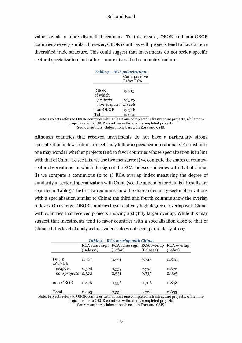
Belt and Road
17
value signals a more diversified economy. To this regard, OBOR and non-OBOR
countries are very similar; however, OBOR countries with projects tend to have a more
diversified trade structure. This could suggest that investments do not seek a specific
sectoral specialization, but rather a more diversified economic structure.
Table 4 – RCA polarization.
Cum. positive Lafay RCA
OBOR 19.713 of which
projects 18.525 non-projects 23.128 non-OBOR 19.588 Total 19.630
Note: Projects refers to OBOR countries with at least one completed infrastructure projects, while non-projects refer to OBOR countries without any completed projects.
Source: authors’ elaborations based on Eora and CSIS.
Although countries that received investments do not have a particularly strong
specialization in few sectors, projects may follow a specialization rationale. For instance,
one may wonder whether projects tend to favor countries whose specialization is in line
with that of China. To see this, we use two measures: i) we compute the shares of country-
sector observations for which the sign of the RCA indexes coincides with that of China;
ii) we compute a continuous (0 to 1) RCA overlap index measuring the degree of
similarity in sectoral specialization with China (see the appendix for details). Results are
reported in Table 5. The first two columns show the shares of country-sector observations
with a specialization similar to China; the third and fourth columns show the overlap
indexes. On average, OBOR countries have relatively high degree of overlap with China,
with countries that received projects showing a slightly larger overlap. While this may
suggest that investments tend to favor countries with a specialization close to that of
China, at this level of analysis the evidence does not seem particularly strong.
Table 5 – RCA overlap with China.
RCA same sign (Balassa)
RCA same sign (Lafay)
RCA overlap (Balassa)
RCA overlap (Lafay)
OBOR 0.527 0,551 0.748 0.870 of which
projects 0.528 0,559 0.752 0.872 non-projects 0.522 0,531 0.737 0.865 non-OBOR 0.476 0,556 0.706 0.848
Total 0.493 0,554 0.720 0.855
Note: Projects refers to OBOR countries with at least one completed infrastructure projects, while non-projects refer to OBOR countries without any completed projects.
Source: authors’ elaborations based on Eora and CSIS.

Belt and Road
18
The above evidence is based on averages of country-sector overlap indexes. As a
check, let us compute country aggregate overlap indicators (see the appendix for details).
Results are qualitatively similar and even stronger, although the degree of overlap is
lower (by construction). OBOR countries overlap relatively more with China, with
countries that received projects showing a particularly high degree of overlap, especially
as measured by the Lafay index.
Table 6 – Aggregate RCA overlap with China.
Aggregate RCA overlap (Balassa)
Aggregate RCA overlap (Lafay)
OBOR 0.400 0.467 of which
projects 0.409 0.496 non-projects 0.374 0.383 non-OBOR 0.299 0.448 Total 0.333 0.454
Note: Projects refers to OBOR countries with at least one completed infrastructure projects, while non-projects refer to OBOR countries without any completed projects.
Source: authors’ elaborations based on Eora and CSIS.
5.3 Trade in intermediate goods
Let us now focus on trade in intermediate goods. We consider the shares of intermediates
in total exports and total imports as well as the composition of intermediate trade,
specifically the shares of total intermediates exported to and imported from China.
Larger shares of intermediates in total trade indicate a stronger participation in GVC,
while the shares of China measure the composition of intermediate trade, which may be
biased towards the country. Descriptive statistics are reported in Table 7. At the world
level, trade in intermediates represents about 71% of total export and 64% of total import
(country-sector average). OBOR countries trade slightly less intermediates, but, non-
surprisingly, they trade more with China. Countries with projects trade more
intermediates, export more to China, but import less from China. This evidence is in line
with the idea that OBOR projects may allow China to develop its suppliers’ network,
freeing internal resources for upgrading, while at the same time helping industrial
development in the recipient countries.
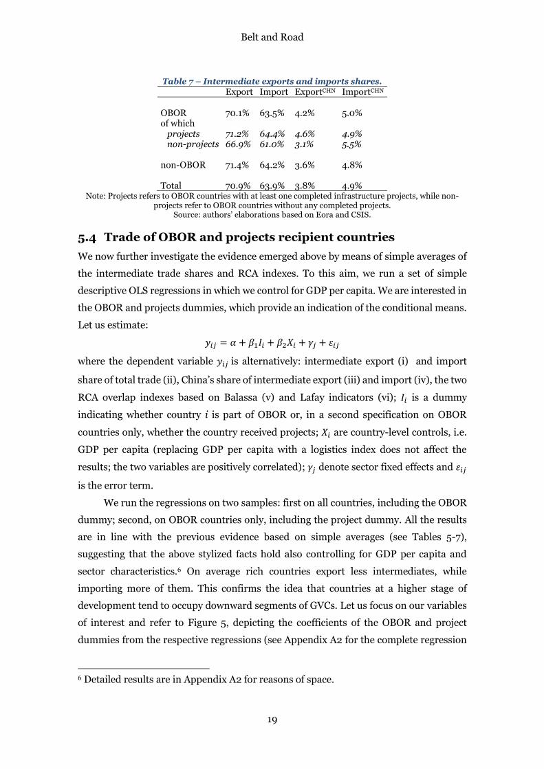
Belt and Road
19
Table 7 – Intermediate exports and imports shares.
Export Import ExportCHN ImportCHN OBOR 70.1% 63.5% 4.2% 5.0% of which projects 71.2% 64.4% 4.6% 4.9% non-projects 66.9% 61.0% 3.1% 5.5%
non-OBOR 71.4% 64.2% 3.6% 4.8%
Total 70.9% 63.9% 3.8% 4.9%
Note: Projects refers to OBOR countries with at least one completed infrastructure projects, while non-projects refer to OBOR countries without any completed projects.
Source: authors’ elaborations based on Eora and CSIS.
5.4 Trade of OBOR and projects recipient countries
We now further investigate the evidence emerged above by means of simple averages of
the intermediate trade shares and RCA indexes. To this aim, we run a set of simple
descriptive OLS regressions in which we control for GDP per capita. We are interested in
the OBOR and projects dummies, which provide an indication of the conditional means.
Let us estimate:
𝑦𝑖𝑗 = 𝛼 + 𝛽1𝐼𝑖 + 𝛽2𝑋𝑖 + 𝛾𝑗 + 𝜀𝑖𝑗
where the dependent variable 𝑦𝑖𝑗 is alternatively: intermediate export (i) and import
share of total trade (ii), China’s share of intermediate export (iii) and import (iv), the two
RCA overlap indexes based on Balassa (v) and Lafay indicators (vi); 𝐼𝑖 is a dummy
indicating whether country i is part of OBOR or, in a second specification on OBOR
countries only, whether the country received projects; 𝑋𝑖 are country-level controls, i.e.
GDP per capita (replacing GDP per capita with a logistics index does not affect the
results; the two variables are positively correlated); 𝛾𝑗 denote sector fixed effects and 𝜀𝑖𝑗
is the error term.
We run the regressions on two samples: first on all countries, including the OBOR
dummy; second, on OBOR countries only, including the project dummy. All the results
are in line with the previous evidence based on simple averages (see Tables 5-7),
suggesting that the above stylized facts hold also controlling for GDP per capita and
sector characteristics.6 On average rich countries export less intermediates, while
importing more of them. This confirms the idea that countries at a higher stage of
development tend to occupy downward segments of GVCs. Let us focus on our variables
of interest and refer to Figure 5, depicting the coefficients of the OBOR and project
dummies from the respective regressions (see Appendix A2 for the complete regression
6 Detailed results are in Appendix A2 for reasons of space.

Belt and Road
20
tables). In the Figure, we see that the OBOR dummy coefficient on intermediate export
is negative while that on import is non-significant, meaning that OBOR countries tend
to export fewer intermediate products than their income level would predict. The project
dummy coefficients on intermediate export and import are both positive, showing that,
contrary to other OBOR countries, those that received projects tend to export and import
more intermediates; indication suggesting that OBOR investments and production
networks are closely related. With respect to the share of China as a destination or as a
source of intermediate products, results indicate that on average rich countries trade
more intermediates with China. This effect is higher for import from China: OBOR
countries export more intermediates to China, but do not import more from China (see
the OBOR dummy coefficients on intermediate export and import with China in Figure
5). This evidence is even stronger for OBOR countries with completed projects. They
export more intermediates to China but import less (the project dummy coefficient is
positive on intermediate export to China while it is negative on intermediate import from
China). This suggests that investments may favor countries that are in a better position
to supply intermediates to China, rather than countries that demand inputs. Finally,
OBOR countries and China have relatively similar specialization; this holds for countries
with projects as well (see the OBOR and project dummy coefficients for RCA overlap in
Figure 5). OBOR investments, thus, tend to reflect China’s comparative advantages,
perhaps in different segments within the same sectors.
Figure 5 – Estimated coefficients of OBOR and projects dummies on different variables.
* p<0.1, ** p<0.05, *** p<0.01; see the appendix for detailed regression tables.
Source: authors’ elaborations based on Eora, CSIS and WDI.
-0.026*-0.008
0.091***
0.019
0.119***0.090***
0.116***
0.162***0.102*
-0.115***
0.092***0.059
IntermediateExport
IntermediateImport
Int. ExportCHN
Int. ImportCHN
RCA overlapBalassa
RCA overlapLafay
Dependent variables
OBOR coeff. proj coeff.

Belt and Road
21
5.5 The intermediate trade networks
The above evidence points towards a role for GVC and production networks in the
distribution of OBOR investment projects. In what follows, we investigate the
configuration of the intermediate trade network of the OBOR countries. To get a clearer,
easier to interpret, figure of the production linkages we present the results for
manufacturing. For the same reason, we exclude minor trade flows.
Figure 6 – World intermediate trade network.
Note: manufacturing sectors, year 2012, flows>0.5% of world trade. Source: authors’ elaborations based on Eora.
The world intermediate trade network, non-surprisingly, clearly displays three
main manufacturing regions: Europe, Asia and North America. These areas have three
main hubs respectively: Germany, China and USA. The centrality of China in the world
production network and, even more so, in the BRI is apparent. In this configuration, the
BRI is likely to reinforce the link between Europe and China, which is dominated by the
China-Germany relation, possibly creating more and new linkages and making the
network more stable, i.e. less sensitive to shocks to specific spokes. The development of
this new linkages, in which China is likely to play a major role, will probably reinforce
the importance of China in the world intermediate trade network.
In the above figure most OBOR countries are absent. This is because their trade
linkages are minor relative to the main world traders. To understand how OBOR
countries connect with the main players, we slightly increase the detail and add them in
Figure 7. OBOR countries tend to distribute into three regions: most (Asian) OBOR
countries, as expected, gravitate around China; (East) European OBOR countries relate
to China through Germany and do not present strong direct linkages with Asia; some
OBOR countries, instead, belong to the Russian subnetwork. Creating significant trade
connections between those countries, and probably with China, might deeply change the

Belt and Road
22
network configuration making all the OBOR countries more central and reducing the
importance of the other regional hubs (Germany, USA, Japan and Russia).
Figure 7 – World intermediate trade network plus main OBOR countries.
Note: manufacturing sectors, year 2012, flows>0.1% of world trade for OBOR countries, >0.5% for others. Source: authors’ elaborations based on Eora and CSIS.
The level of details of the previous figures, focused on the world network, shows
that many OBOR countries do not share strong direct trade linkages. It is then useful to
change the scale and focus on the OBOR intermediate trade sub-network in order to see
the main linkages between OBOR countries, which although small on the world scale,
may represent the basis for further development of trade thanks to the BRI. Figure 8
shows, again, the centrality of China.
Figure 8 – Intermediate trade network of OBOR countries.
Note: manufacturing sectors, year 2012, flows >0.5% of total regional trade. Source: authors’ elaborations based on Eora and CSIS.
Eastern Asian countries are relatively well connected among themselves, with most
of them supplying manufacturing inputs to China. Russia also is a major supplier of
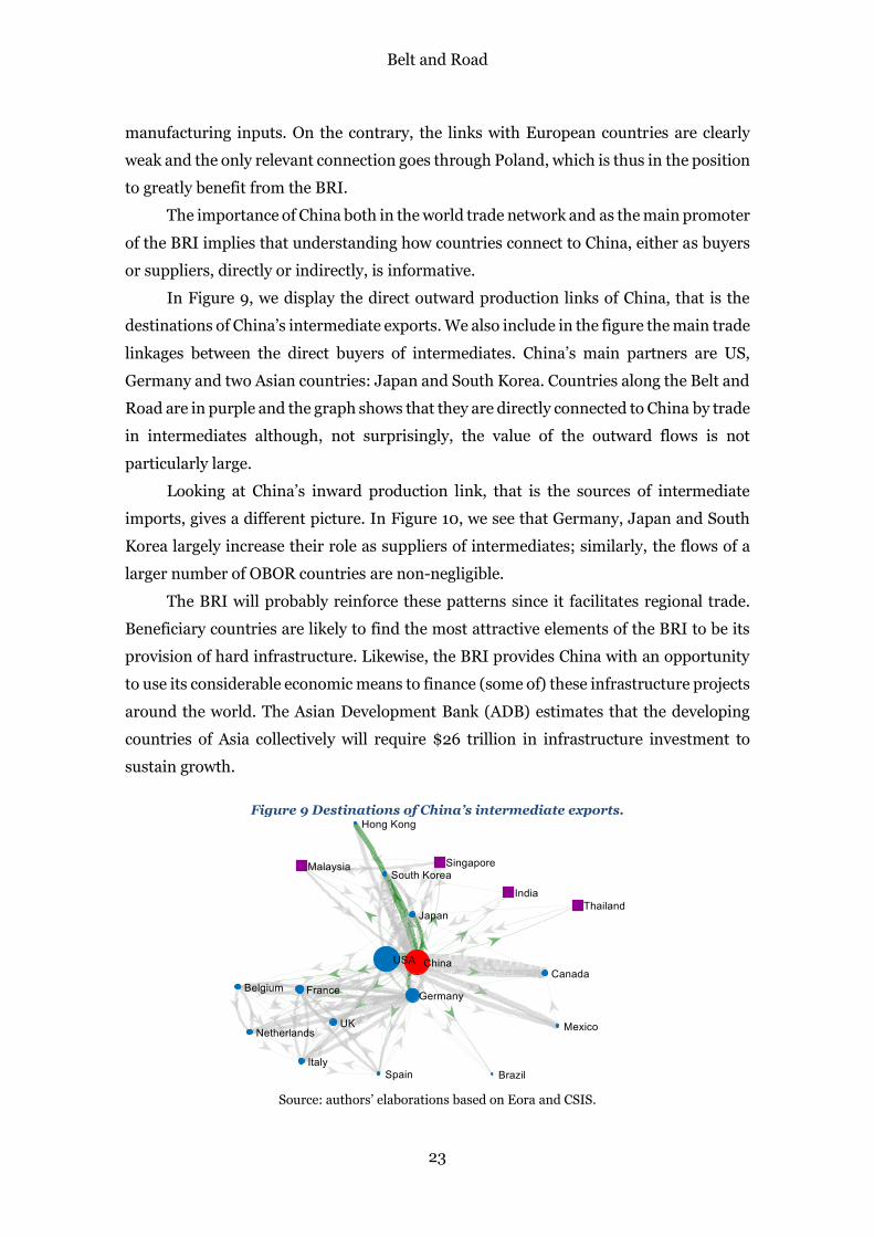
Belt and Road
23
manufacturing inputs. On the contrary, the links with European countries are clearly
weak and the only relevant connection goes through Poland, which is thus in the position
to greatly benefit from the BRI.
The importance of China both in the world trade network and as the main promoter
of the BRI implies that understanding how countries connect to China, either as buyers
or suppliers, directly or indirectly, is informative.
In Figure 9, we display the direct outward production links of China, that is the
destinations of China’s intermediate exports. We also include in the figure the main trade
linkages between the direct buyers of intermediates. China’s main partners are US,
Germany and two Asian countries: Japan and South Korea. Countries along the Belt and
Road are in purple and the graph shows that they are directly connected to China by trade
in intermediates although, not surprisingly, the value of the outward flows is not
particularly large.
Looking at China’s inward production link, that is the sources of intermediate
imports, gives a different picture. In Figure 10, we see that Germany, Japan and South
Korea largely increase their role as suppliers of intermediates; similarly, the flows of a
larger number of OBOR countries are non-negligible.
The BRI will probably reinforce these patterns since it facilitates regional trade.
Beneficiary countries are likely to find the most attractive elements of the BRI to be its
provision of hard infrastructure. Likewise, the BRI provides China with an opportunity
to use its considerable economic means to finance (some of) these infrastructure projects
around the world. The Asian Development Bank (ADB) estimates that the developing
countries of Asia collectively will require $26 trillion in infrastructure investment to
sustain growth.
Figure 9 Destinations of China’s intermediate exports.
Source: authors’ elaborations based on Eora and CSIS.
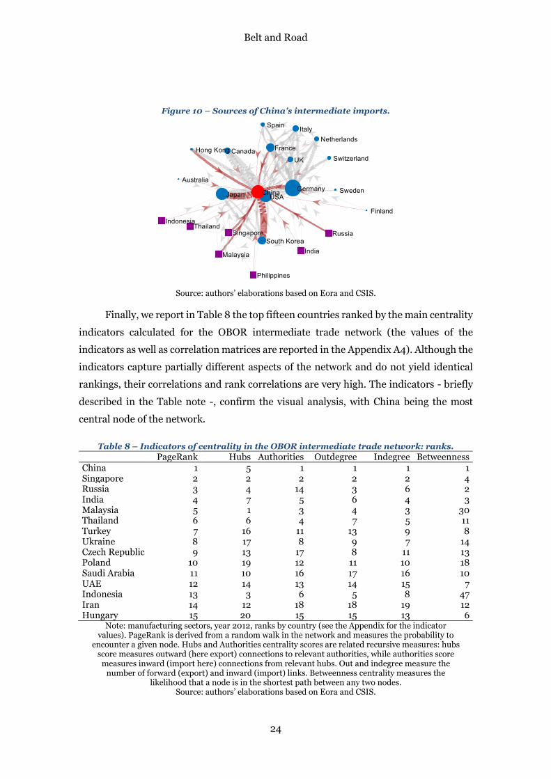
Belt and Road
24
Figure 10 – Sources of China’s intermediate imports.
Source: authors’ elaborations based on Eora and CSIS.
Finally, we report in Table 8 the top fifteen countries ranked by the main centrality
indicators calculated for the OBOR intermediate trade network (the values of the
indicators as well as correlation matrices are reported in the Appendix A4). Although the
indicators capture partially different aspects of the network and do not yield identical
rankings, their correlations and rank correlations are very high. The indicators - briefly
described in the Table note -, confirm the visual analysis, with China being the most
central node of the network.
Table 8 – Indicators of centrality in the OBOR intermediate trade network: ranks.
PageRank Hubs Authorities Outdegree Indegree Betweenness China 1 5 1 1 1 1 Singapore 2 2 2 2 2 4 Russia 3 4 14 3 6 2 India 4 7 5 6 4 3 Malaysia 5 1 3 4 3 30 Thailand 6 6 4 7 5 11 Turkey 7 16 11 13 9 8 Ukraine 8 17 8 9 7 14 Czech Republic 9 13 17 8 11 13 Poland 10 19 12 11 10 18 Saudi Arabia 11 10 16 17 16 10 UAE 12 14 13 14 15 7 Indonesia 13 3 6 5 8 47 Iran 14 12 18 18 19 12 Hungary 15 20 15 15 13 6
Note: manufacturing sectors, year 2012, ranks by country (see the Appendix for the indicator values). PageRank is derived from a random walk in the network and measures the probability to
encounter a given node. Hubs and Authorities centrality scores are related recursive measures: hubs score measures outward (here export) connections to relevant authorities, while authorities score
measures inward (import here) connections from relevant hubs. Out and indegree measure the number of forward (export) and inward (import) links. Betweenness centrality measures the
likelihood that a node is in the shortest path between any two nodes. Source: authors’ elaborations based on Eora and CSIS.

Belt and Road
25
5.6 Intra-industry trade
Let us now focus on intra-industry trade (IIT), particularly relevant since China is
a major importer of manufactured inputs used in the production of its own exports. In
this context, intra-industry linkages typically constitute the larger share of trade,
especially with broader sector definition (as in Eora). By investigating IIT, we thus keep
track of two broad and interrelated phenomena, i.e. product differentiation and GVC, for
what regards trade flows within broadly-defined sectors. The most commonly used IIT
indicator is the Grubel & Lloyd (1971, 1975) index (GL; see the Appendix A3 for details).
Plotting GL against GDP per capita, as in Figure 11, reveals a positive correlation: richer
countries tend to trade more within sectors. In the figure, however, we see that OBOR
countries tend to form an inverted-U-shape: middle-income OBOR countries are more
involved into intra-industry trade than their income level would imply-
In Figure 12, we consider countries that received projects. IIT does not seem
related to the number of projects, while we clearly see that countries more involved in
IIT get larger investments.
Figure 11 – Intra-industry trade against GDP per capita.
Note: the graph uses a logit transformation of the GL index. Source: authors’ elaborations based on Eora, CSIS and WDI.
Figure 12 – IIT and number and average value of OBOR projects.
Source: authors’ elaborations based on Eora and CSIS.
-4-2
02
6 7 8 9 10 11 12Log GDP per capita 2012
95% CI predicted GL12_logit
GL12_logit 95% CI
predicted GL12_logit GL12_logit
-4-2
02
0 5 10 15 20 25Total Number of Completed Projects between 2012 and 2018
95% CI predicted GL12_logit
GL12_logit
-4-2
02
16 18 20 22 24Log average value of projects
95% CI predicted GL12_logit
GL12_logit
Belt and Road
26
5.7 Export and import sophistication
One of the main issues of countries’ participation in GVC regards their ability to reap the
benefits and upgrade. The composition of the trade bundle provides a first indication of
the capability of a country to secure and supply better, more sophisticated products, and
ultimately occupy a more valuable position within the value chain. One indication of this
is provided by a sophistication index developed by Hausmann et al. (2007) and Rodrik
(2006), which captures the average level of income implied by a country’s trade bundle.
Non-surprisingly, rich countries tend to have more sophisticated export and import
bundles, i.e. they import and, especially, export more advanced products. As a
consequence, a similar indication is obtained by considering similarity indexes between
a country’s export bundle and the export bundle of richer countries (Schott, 2008; Wang
& Wei, 2008). In what follows, we investigate export and import sophistication of OBOR
countries. Our approach is similar to Marvasi (2013).
Figure 13 shows export and import sophistication. As expected, we see that exports
sophistication is more variable than import sophistication, reflecting more closely the
income level. Import sophistication tends to be higher than export sophistication,
indicating that less developed countries tend to import relatively sophisticated products
exporting less sophisticated ones, while more advanced countries trade highly
sophisticated products. Consequently, the gap between import and export sophistication
decreases with income. Rodrik (2006) and subsequent studies highlight the fact that
China’s export is particularly sophisticated conditional on its level of development. The
figure suggests that we can generalize this finding to middle-income OBOR countries. To
this regard, the BRI may contribute to create a group of interconnected sophisticated
exporters. Marvasi (2013) shows that China’s surprisingly high level of sophistication is
due to intermediates, for which export sophistication surpassed import sophistication in
the early 2000s. Over time, the increasing export sophistication signals China’s
upgrading. However, such improvement also implies that, relative to its income, China
is becoming “less special”. This adds to the possibility that the BRI can help China
upgrade its suppliers’ network.

Belt and Road
27
Figure 13 – Export and import sophistication.
Source: authors’ elaborations based on Eora, CSIS and WDI.
Focusing on OBOR countries with completed projects (Figure 14), we see that
countries that obtained more projects tend to have less sophisticated exports and more
sophisticated imports. On the contrary, more sophisticated exporters received projects
of higher value, mostly in line with their higher income level.
We investigate further the export sophistication of OBOR countries by means of
simple OLS regressions. The inverted-U shape of the relations between export
sophistication (expy) and income for OBOR countries highlighted above is confirmed.
Other things equal, OBOR countries gain sophistication faster, but also reach a
maximum earlier at middle income levels. Focusing on OBOR countries only, those with
projects shows a similar, if not stronger, pattern: middle-income countries with projects
are more sophisticated, other things equal.
Figure 14 – Sophistication and number and average value of OBOR projects.
Source: authors’ elaborations based on Eora and CSIS.
99
.29
.49
.69
.8
6 7 8 9 10 11 12Log GDP per capita 2012
95% CI predicted ln_expy12
ln_expy12 95% CI
predicted ln_expy12 ln_expy12
9.4
9.5
9.6
9.7
9.8
9.9
6 7 8 9 10 11 12Log GDP per capita 2012
95% CI predicted ln_impy12
ln_impy12 95% CI
predicted ln_impy12 ln_impy12
99
.29
.49
.69
.8
0 5 10 15 20 25Total Number of Completed Projects between 2012 and 2018
95% CI predicted ln_expy12
ln_expy12 predicted ln_impy12
ln_impy12
99
.29
.49
.69
.8
16 18 20 22 24Log average value of projects
95% CI predicted ln_expy12
ln_expy12 predicted ln_impy12
ln_impy12
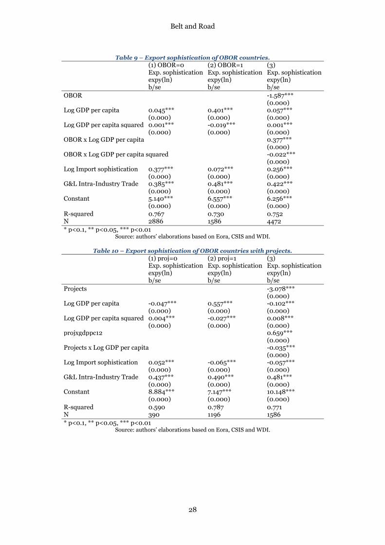
Belt and Road
28
Table 9 – Export sophistication of OBOR countries.
(1) OBOR=0 (2) OBOR=1 (3)
Exp. sophistication expy(ln)
Exp. sophistication expy(ln)
Exp. sophistication expy(ln)
b/se b/se b/se OBOR -1.587***
(0.000) Log GDP per capita 0.045*** 0.401*** 0.057***
(0.000) (0.000) (0.000) Log GDP per capita squared 0.001*** -0.019*** 0.001***
(0.000) (0.000) (0.000) OBOR x Log GDP per capita 0.377***
(0.000) OBOR x Log GDP per capita squared -0.022***
(0.000) Log Import sophistication 0.377*** 0.072*** 0.256***
(0.000) (0.000) (0.000) G&L Intra-Industry Trade 0.385*** 0.481*** 0.422***
(0.000) (0.000) (0.000) Constant 5.140*** 6.557*** 6.256***
(0.000) (0.000) (0.000) R-squared 0.767 0.730 0.752 N 2886 1586 4472 * p<0.1, ** p<0.05, *** p<0.01
Source: authors’ elaborations based on Eora, CSIS and WDI.
Table 10 – Export sophistication of OBOR countries with projects.
(1) proj=0 (2) proj=1 (3)
Exp. sophistication expy(ln)
Exp. sophistication expy(ln)
Exp. sophistication expy(ln)
b/se b/se b/se Projects -3.078***
(0.000) Log GDP per capita -0.047*** 0.557*** -0.102***
(0.000) (0.000) (0.000) Log GDP per capita squared 0.004*** -0.027*** 0.008***
(0.000) (0.000) (0.000) projxgdppc12 0.659***
(0.000) Projects x Log GDP per capita -0.035***
(0.000) Log Import sophistication 0.052*** -0.065*** -0.057***
(0.000) (0.000) (0.000) G&L Intra-Industry Trade 0.437*** 0.490*** 0.481***
(0.000) (0.000) (0.000) Constant 8.884*** 7.147*** 10.148***
(0.000) (0.000) (0.000) R-squared 0.590 0.787 0.771 N 390 1196 1586 * p<0.1, ** p<0.05, *** p<0.01
Source: authors’ elaborations based on Eora, CSIS and WDI.

Belt and Road
29
6 Econometric analysis of project decisions
Let us now investigate the drivers of projects investments decision. Our aim is to
understand to what extent intermediate trade represents an important factor for the
involvement into the BRI, and for the selection and distribution of projects. We first start
with what determines whether a country is selected to be part of the Belt and Road
Initiative, then move to investment project selection and finally investigate investment
value. The underlying equation is:
𝑦𝑖 = 𝛼 + 𝛽1𝐸𝑥𝑝𝑗𝑖 + 𝛽2𝐼𝑚𝑝𝑗𝑖 + 𝛽3𝐸𝑥𝑝𝑗𝑖𝐶𝐻𝑁 + 𝛽4𝐼𝑚𝑝𝑗𝑖
𝐶𝐻𝑁 + 𝛽5𝑅𝐶𝐴𝑗𝑖 + 𝜷6′𝒁𝑖 + 𝜀𝑖
where the dependent variable 𝑦𝑖 is either: i) a dummy variable indicating whether
country i is an OBOR country or not; ii) the number of completed projects; iii) total value
of investments in the country (in logarithm). Five key trade variables are central to our
analysis. 𝐸𝑥𝑝𝑗𝑖 is the intermediate export share of sector j over total export of country i.
Likewise, 𝐼𝑚𝑝𝑗𝑖 is the intermediate import share of sector j over total import of country
i. 𝐸𝑥𝑝𝑗𝑖𝐶𝐻𝑁 is the share of China on total intermediate export of country i in sector j.
Similarly, 𝐼𝑚𝑝𝑗𝑖𝐶𝐻𝑁 is the share of China on total intermediate import of country i in sector
j. The variable 𝑅𝐶𝐴𝑗𝑖 denotes the sector-level revealed comparative advantage overlap
between country i and China. Finally, the vector 𝒁𝑖 includes a series of country-level
control variables such as GDP per capita (in log), trade logistics index, export and import
sophistication (in log) as well as measures of intra-industry trade. Finally, 𝜀𝑖 is an
idiosyncratic error term clustered at the sector-level.
The cross-sectional nature of the data requires us to exclude contemporaneous
correlation between variables. To overcome this, all independent variables including
controls are lagged at year 2012. In this way, our econometric design analyses pre-BRI
trade relations mechanism that explains selection and distribution of infrastructure
projects.
6.1 What characterizes OBOR countries
Table 11 reports estimates of the above regression model in which the dependent variable
is the OBOR dummy. The share of intermediate exports and imports are not statistically
significant as determinants of being selected into the Belt and Road Initiative. However,
the share of intermediate export to China increases the probability of a country being
selected into the BRI. Surprisingly, intermediate import from China is not statistically
significant to determine selection into BRI. In addition, sector-level overlapping RCA
positively determines the probability of selection into BRI. To exclude results being
driven by potential multi-correlation, we also estimate the equation separating the trade
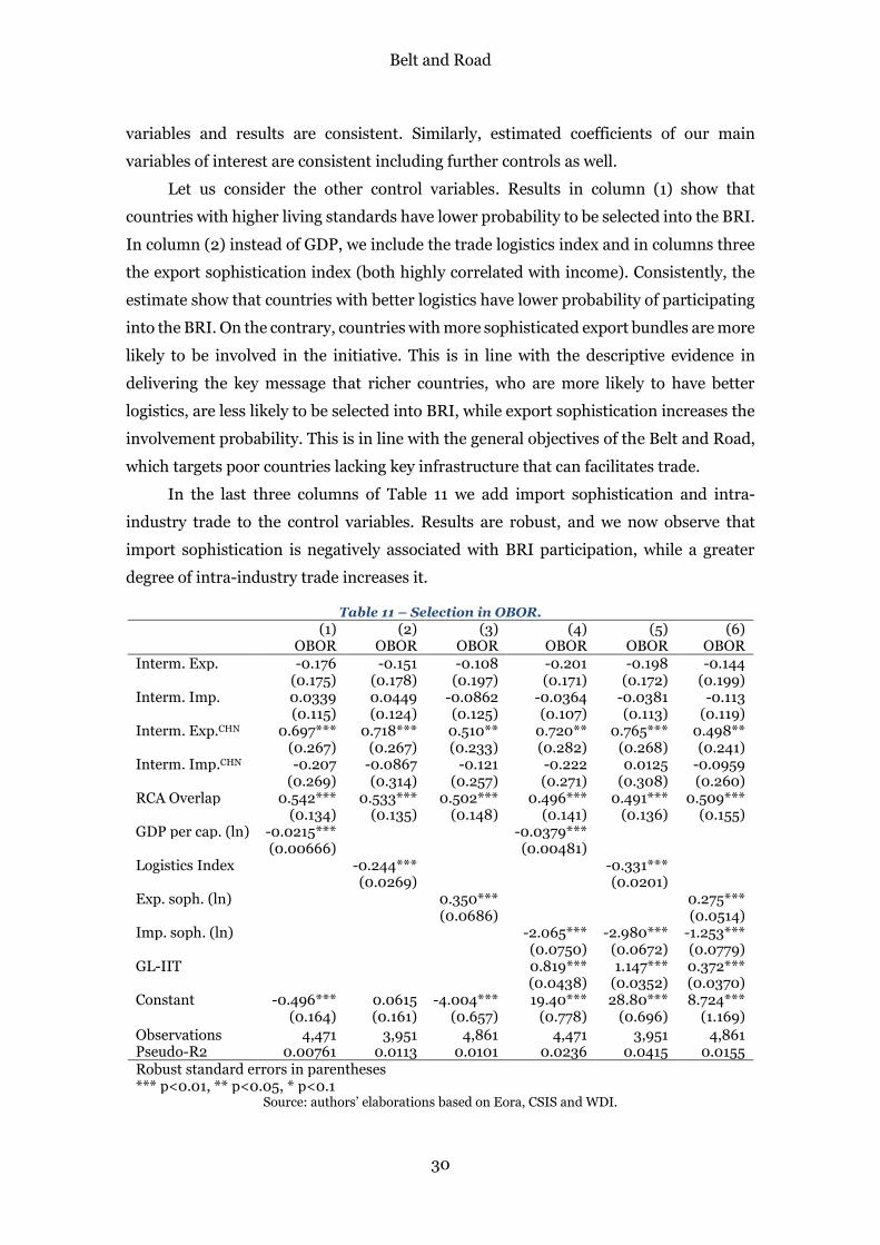
Belt and Road
30
variables and results are consistent. Similarly, estimated coefficients of our main
variables of interest are consistent including further controls as well.
Let us consider the other control variables. Results in column (1) show that
countries with higher living standards have lower probability to be selected into the BRI.
In column (2) instead of GDP, we include the trade logistics index and in columns three
the export sophistication index (both highly correlated with income). Consistently, the
estimate show that countries with better logistics have lower probability of participating
into the BRI. On the contrary, countries with more sophisticated export bundles are more
likely to be involved in the initiative. This is in line with the descriptive evidence in
delivering the key message that richer countries, who are more likely to have better
logistics, are less likely to be selected into BRI, while export sophistication increases the
involvement probability. This is in line with the general objectives of the Belt and Road,
which targets poor countries lacking key infrastructure that can facilitates trade.
In the last three columns of Table 11 we add import sophistication and intra-
industry trade to the control variables. Results are robust, and we now observe that
import sophistication is negatively associated with BRI participation, while a greater
degree of intra-industry trade increases it.
Table 11 – Selection in OBOR.
(1) (2) (3) (4) (5) (6) OBOR OBOR OBOR OBOR OBOR OBOR Interm. Exp. -0.176 -0.151 -0.108 -0.201 -0.198 -0.144
(0.175) (0.178) (0.197) (0.171) (0.172) (0.199) Interm. Imp. 0.0339 0.0449 -0.0862 -0.0364 -0.0381 -0.113
(0.115) (0.124) (0.125) (0.107) (0.113) (0.119) Interm. Exp.CHN 0.697*** 0.718*** 0.510** 0.720** 0.765*** 0.498**
(0.267) (0.267) (0.233) (0.282) (0.268) (0.241) Interm. Imp.CHN -0.207 -0.0867 -0.121 -0.222 0.0125 -0.0959
(0.269) (0.314) (0.257) (0.271) (0.308) (0.260) RCA Overlap 0.542*** 0.533*** 0.502*** 0.496*** 0.491*** 0.509***
(0.134) (0.135) (0.148) (0.141) (0.136) (0.155) GDP per cap. (ln) -0.0215*** -0.0379*** (0.00666) (0.00481) Logistics Index -0.244*** -0.331*** (0.0269) (0.0201) Exp. soph. (ln) 0.350*** 0.275***
(0.0686) (0.0514) Imp. soph. (ln) -2.065*** -2.980*** -1.253***
(0.0750) (0.0672) (0.0779) GL-IIT 0.819*** 1.147*** 0.372***
(0.0438) (0.0352) (0.0370) Constant -0.496*** 0.0615 -4.004*** 19.40*** 28.80*** 8.724***
(0.164) (0.161) (0.657) (0.778) (0.696) (1.169) Observations 4,471 3,951 4,861 4,471 3,951 4,861 Pseudo-R2 0.00761 0.0113 0.0101 0.0236 0.0415 0.0155 Robust standard errors in parentheses *** p<0.01, ** p<0.05, * p<0.1
Source: authors’ elaborations based on Eora, CSIS and WDI.

Belt and Road
31
6.2 The number of completed projects
We now concentrate on the subset of OBOR countries to answer how do pre-existing
trade relations explain the number of completed projects, subject to the fact that a
country is participating in initiative. Our dependent variable is the number of completed
projects, a count variable. We thus estimate a Poisson model. Results are reported in
Table 12. While intermediate trade shares do not affect OBOR participation, they matter
for the number of projects received. The share of intermediate export over total export
reduces the number of infrastructure projects completed in an OBOR country, while the
opposite holds for intermediate import. Countries that import high quantities of
intermediate inputs are likely to be more integrated in the network of global value chain
production; these countries are likely to receive more infrastructure projects than their
peers. But trade relations with China are also relevant both for participation into the
initiative and for the number of projects received. Intermediate trade with China is
statistically significant and positively correlated with the number of completed projects.
This seems to suggest that OBOR countries supplying intermediary inputs to China
receive more infrastructure projects than countries supplying intermediate inputs to the
rest of the world. Similarly, a higher degree of overlap with China in terms of revealed
comparative advantage positively affects the number of completed projects.
Adding per capita GDP and trade logistics index as control variables, the
coefficients of both variables indicate that countries with high living standards and good
trade logistics infrastructure will have a smaller number of completed infrastructure
projects. This enhances our previous assertion that the Belt and Road Initiative targets
developing countries with high trade potentials. Export sophistication negatively
correlates with the number of completed projects. Note that export sophistication is
positively associated with participation into the BRI, but negatively with the number of
projects. To reconcile these findings, recall that richer countries are generally more likely
to export sophisticated products and could be able to provide for their own
infrastructure. Finally, intra-industry trade positively correlates with the number
completed projects.

Belt and Road
32
Table 12 – Selection of project recipients.
(1) (2) (3) (4) (5) (6)
Projects number
Projects number
Projects number
Projects number
Projects number
Projects number
Interm. Exp. -0.479*** -0.284** -0.291** -0.402*** -0.282** -0.336***
(0.113) (0.120) (0.135) (0.0979) (0.119) (0.126) Interm. Imp. 0.513*** 0.306*** 0.365*** 0.463*** 0.285*** 0.381***
(0.0754) (0.0888) (0.0938) (0.0702) (0.0882) (0.0974) Interm. Exp.CHN 0.595** 0.963*** 0.781*** 0.728*** 1.005*** 0.887***
(0.244) (0.254) (0.268) (0.230) (0.249) (0.251) Interm. Imp.CHN 0.187 0.370* 0.720*** -0.0713 0.431** 0.662***
(0.187) (0.207) (0.219) (0.156) (0.216) (0.205) RCA Overlap 0.403*** 0.261** 0.396*** 0.259*** 0.229** 0.323***
(0.0909) (0.119) (0.122) (0.0884) (0.116) (0.106) GDP per cap. (ln) -0.371*** -0.454***
(0.00645) (0.00590) Logistics Index -0.105*** -0.162***
(0.0167) (0.0148) Exp. soph. (ln) -0.924*** -1.993***
(0.0441) (0.0591) Imp. soph. (ln) 1.418*** -0.177*** 0.237***
(0.0691) (0.0499) (0.0549) GL-IIT 0.737*** 0.323*** 1.420***
(0.0331) (0.0285) (0.0295) Constant 4.457*** 1.721*** 10.04*** -8.888*** 3.466*** 17.25***
(0.110) (0.0890) (0.411) (0.664) (0.511) (0.659) Observations 1,586 1,508 1,612 1,586 1,508 1,612 Robust standard errors in parentheses *** p<0.01, ** p<0.05, * p<0.1
Source: authors’ elaborations based on Eora, CSIS and WDI.
6.3 The value of completed projects
Lastly, we examine whether trade relations variables explain the value of the completed
projects. We estimate our regression equation by means of OLS using the log of the value
of infrastructure projects as dependent variable. Table 13 reports the.
The export and import shares of intermediate trade, in line with the previous
regressions for the number of projects, display a negative and positive coefficient, both
statistically significant at the 1% level. A stronger involvement in GVC as importer of
intermediates rather than as exporter is associated with larger investment values.
Intermediate trade with China (either export or import), relevant for the number
of projects, also has some impact on the value invested, at least on the import side. The
coefficient of intermediate export to China remains consistently positive but non-
significant in all the specifications, while the coefficient of intermediate import from
China is significant in columns (3) to (6). One potential explanation is that, while two-
way intermediate trade with China positively affects the number of projects a country
receives, the total value invested follows a different rationale. The change in the sign of
income, logistics and export sophistication seems to support this interpretation. OBOR
investments seem to follow two different motivations: on average, less developed
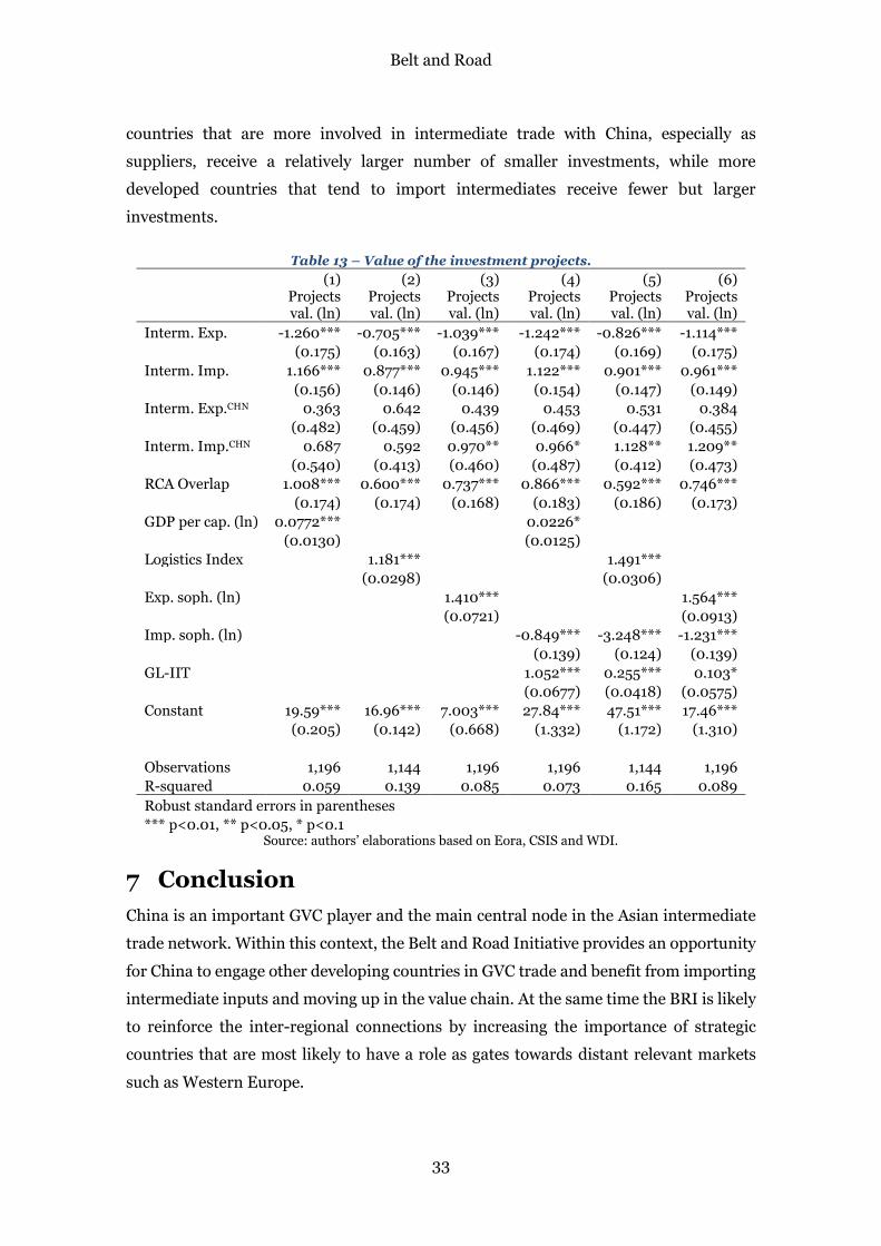
Belt and Road
33
countries that are more involved in intermediate trade with China, especially as
suppliers, receive a relatively larger number of smaller investments, while more
developed countries that tend to import intermediates receive fewer but larger
investments.
Table 13 – Value of the investment projects.
(1) (2) (3) (4) (5) (6)
Projects val. (ln)
Projects val. (ln)
Projects val. (ln)
Projects val. (ln)
Projects val. (ln)
Projects val. (ln)
Interm. Exp. -1.260*** -0.705*** -1.039*** -1.242*** -0.826*** -1.114***
(0.175) (0.163) (0.167) (0.174) (0.169) (0.175)
Interm. Imp. 1.166*** 0.877*** 0.945*** 1.122*** 0.901*** 0.961***
(0.156) (0.146) (0.146) (0.154) (0.147) (0.149)
Interm. Exp.CHN 0.363 0.642 0.439 0.453 0.531 0.384
(0.482) (0.459) (0.456) (0.469) (0.447) (0.455)
Interm. Imp.CHN 0.687 0.592 0.970** 0.966* 1.128** 1.209**
(0.540) (0.413) (0.460) (0.487) (0.412) (0.473)
RCA Overlap 1.008*** 0.600*** 0.737*** 0.866*** 0.592*** 0.746***
(0.174) (0.174) (0.168) (0.183) (0.186) (0.173)
GDP per cap. (ln) 0.0772*** 0.0226*
(0.0130) (0.0125) Logistics Index 1.181*** 1.491***
(0.0298) (0.0306) Exp. soph. (ln) 1.410*** 1.564***
(0.0721) (0.0913)
Imp. soph. (ln) -0.849*** -3.248*** -1.231***
(0.139) (0.124) (0.139)
GL-IIT 1.052*** 0.255*** 0.103*
(0.0677) (0.0418) (0.0575)
Constant 19.59*** 16.96*** 7.003*** 27.84*** 47.51*** 17.46***
(0.205) (0.142) (0.668) (1.332) (1.172) (1.310)
Observations 1,196 1,144 1,196 1,196 1,144 1,196
R-squared 0.059 0.139 0.085 0.073 0.165 0.089
Robust standard errors in parentheses
*** p<0.01, ** p<0.05, * p<0.1 Source: authors’ elaborations based on Eora, CSIS and WDI.
7 Conclusion
China is an important GVC player and the main central node in the Asian intermediate
trade network. Within this context, the Belt and Road Initiative provides an opportunity
for China to engage other developing countries in GVC trade and benefit from importing
intermediate inputs and moving up in the value chain. At the same time the BRI is likely
to reinforce the inter-regional connections by increasing the importance of strategic
countries that are most likely to have a role as gates towards distant relevant markets
such as Western Europe.
Belt and Road
34
Infrastructure investments (new roads, railways, ports and communications, see
table A1 in the Appendix) reduce transport costs and facilitate the movement of goods
and people. Along the OBOR corridors, firms will be able to better coordinate production
and the division of labor across regions. Landlocked economies will benefit from easier
access to important routes. For several of them, participating in GVCs can help a
transition from being a supplier of natural resources and raw materials to becoming a
manufacturer of goods and services. More generally, developing countries involved in
the BRI are likely to be strongly affected by Chinese investments as the returns even to
relatively small projects are likely to be large. In a network perspective strengthening the
weak links is likely to make the entire network more stable. A similar view is in Derudder
et al. (2018). This is beneficial to the regional GVC and helps China building a reliable
base of suppliers. Based on descriptive, graphical and statistical evidence, we claim that
BRI related investments seem to favor large and relatively poor countries, but richer
countries get larger investments. Countries receiving projects have a relatively more
diversified export structure than their peers and, more importantly for our study, their
specialization tends to overlap more with the specialization of China. This is an
interesting and novel finding, so far to our knowledge not investigated. It triggered
further inquiry on the level of GVCs involvement of the BRI countries. We find that more
projects are completed in countries that are more involved in GVC as suppliers of
intermediates to China. If one studies the trade networks, it emerges that China is the
center of the intermediate trade network of OBOR countries, with some countries better
positioned to represent crucial links to other regions.
In summary, our findings highlight that OBOR investments are closely related to
trade patterns and GVC considerations. A simple econometric exercise allows us to
characterize the BRI countries and to suggest how the pre-existing trade relations and
specialization can explain the number and value of infrastructural investments. BRI
countries are getting more involved into production networks, since they provide a
reliable base of suppliers to China, which in turn may able to upgrade its productions
and possibly alleviate its problems of overcapacity.
It is interesting to note that most of the countries where many and larger projects
have been completed display a specialization that is relatively similar to that of China.
We speculate that projects allocation is likely to reinforce China’s comparative
advantages and upgrade its productions by building on the specialization of other
countries in the same sectors on different phases. Opportunities are there, along the “silk
road”. Policies in the different countries should be targeted at exploiting them.

Belt and Road
35
References
Amighini, A. (2017). China’s Belt and Road: A Game Changer? (A. Amighini, Ed.) (1st ed.). Milano: ISPI. http://doi.org/10.19201/ispichinasbelt
Balassa, B. (1965). Trade Liberalisation and “Revealed” Comparative Advantage. The Manchester School. http://doi.org/10.1111/j.1467-9957.1965.tb00050.x
Banerjee, D. (2016). China’s One Belt One Road Initiative – An Indian Perspective. ISEAS Yusof Ishak Institute, Perspective, (14), 1–10.
Baniya, S., Rocha, N., & Ruta, M. (2019). Trade Effects of the New Silk Road. A Gravity Analysis. World Bank Policy Research Working Paper, 8694(January).
Barisitz, S., & Radzyner, A. (2017a). The New Silk Road, part I: a stocktaking and economic assessment. Focus on European Economic Integration, Oesterreichische Nationalbank (Austrian Central Bank), (Q3), 8–31.
Barisitz, S., & Radzyner, A. (2017b). The New Silk Road, part II: implications for Europe. Focus on European Economic Integration, Oesterreichische Nationalbank (Austrian Central Bank), (Q4), 70–81.
Boffa, M. (2018). Trade Linkages Between the Belt and Road Economies. World Bank Policy Research Working Paper, 8423(May).
Bustos, P. (2018). Exposure of Belt and Road Economies to China Trade Shocks. World Bank Policy Research Working Paper, 8503(June).
Cai, P. (2017). Understanding China’s Belt and Road Initiative. Lowy Institute, (March), 26. Retrieved from https://www.lowyinstitute.org/sites/default/files/documents/Understanding China’s Belt and Road Initiative_WEB_1.pdf
Chen, M. X., & Lin, C. (2018). Foreign Investment across the Belt and Road. Patterns, Determinants and Effects. Wolrd Bank Policy Research Working Paper, (October).
Cheng, L. K. (2016). Three questions on China’s “Belt and Road Initiative.” China Economic Review, 40, 309–313. http://doi.org/10.1016/j.chieco.2016.07.008
de Soryres, F., Mulabdic, A., Murray, S., Rocha, N., & Ruta, M. (2018). How Much Will the Belt and Road Initiative Reduce Trade Costs? World Bank Policy Research Working Paper, 8614(October).
Derudder, B., Liu, X., & Kunaka, C. (2018). Connectivity Along Overland Corridors of the Belt and Road initiative. World Bank MTI Global Practice Discussion Paper, 6(October), 2018.
Du, J., & Zhang, Y. (2018). Does One Belt One Road initiative promote Chinese overseas direct investment? China Economic Review.
Enderwick, P. (2018). The economic growth and development effects of China’s One Belt, One Road Initiative. Strategic Change, 27(5), 447–454. http://doi.org/10.1002/jsc.2229
Garcia-Herrero, A., & Xu, J. (2017). China’s Belt and Road Initiative: Can Europe Expect Trade Gains? China and World Economy, 25(6), 84–99. http://doi.org/10.1111/cwe.12222
Ghossein, T., Hoekman, B., & Shingal, A. (2018). Public Procurement in the Belt and Road initiative. Wolrd Bank MTI Global Practice Discussion Paper, 10(December).
Grubel, H. G., & Lloyd, P. J. (1971). The Empirical Measurement of Intra‐Industry Trade. Economic Record. http://doi.org/10.1111/j.1475-4932.1971.tb00772.x
Grubel, H. G., & Lloyd, P. J. (1975). Intra-Industry Trade: The Theory and Measurement of International Trade in Differentiated Products. The Economic Journal. http://doi.org/10.1007/s13277-014-2626-1
Hausmann, R., Hwang, J., & Rodrik, D. (2007). What You Export Matters. Journal of Economic Growth, (12), 1–25. http://doi.org/10.2139/ssrn.896243
Belt and Road
36
Huang, Y. (2016). Understanding China’s Belt & Road Initiative: Motivation, framework and assessment. China Economic Review.
Johns, M. B., Clarke, J. L., Kerswell, C., & McLinden, G. (2018). Trade Facilitation Challenges and Reforms Priorities for Maximizing the Impact of the Belt and Road Initiative. World Bank MTI Global Practice Discussion Paper, September(4).
Kelegama, S. (2014). China-Sri Lanka economic relations: An overview. China Report. http://doi.org/10.1177/0009445514523646
Lafay, G. (1992). The Measurement of Revealed Comparative Advantage. In International Trade Modelling.
Lobyrev, V., Tikhomirov, A., Tsukarev, T., & Vinokurov, E. (2018). Belt and Road Transport Corridors: Barriers and Investments. Centre for Integration Studies, Eurasian Development Bank.
Lu, H., Rohr, C., Hafner, M., & Knack, A. (2018). China Belt and Road Initiative Measuring the impact of improving transport connectivity on international trade in the region-a proof-of-concept study. RAND Europe. http://doi.org/10.7249/RR2625
Marvasi, E. (2013). The sophistication of China’s exports, imports and intermediate products. In The Chinese Economy: Recent Trends and Policy Issues (pp. 181–209). http://doi.org/10.1007/978-3-642-28638-4_9
Nataraj, G., & Sekhani, R. (2015). China’s One Belt One Road: An Indian Perspective. Economic & Political Weekly, 50(49), 67–71.
Ramasamy, B., Yeung, M., Utoktham, C., & Duval, Y. (2017). Trade and trade facilitation along the Belt and Road Initiative corridors. Asia-Pacific Research and Training Network on Trade (ARTNeT) Working Paper Series, (172).
Rodrik, D. (2006). What’s So Special about China’s Exports? China &World Economy, 14(5), 1–19. http://doi.org/10.1007/s11745-004-1336-x
Schott, P. K. (2008). The relative sophistication of Chinese exports. Economic Policy. Retrieved from http://onlinelibrary.wiley.com/doi/10.1111/j.1468-0327.2007.00195.x/full
Villafuerte, J., Corong, E., & Zhuang, J. (2016). The One Belt, One Road Initiative - Impact on Trade and Growth. 19th Annual Conference on Global Economic Analysis, 1–30.
Vinokurov, E., Lobyrev, V., Tikhomirov, A., & Tsukarev, T. (2018). Silk Road Transport Corridors: Assessment of Trans-EUEU Freight Traffic growth Potential. Centre for Integration Studies, Eurasian Development Bank.
Wang, H., & Miao, L. (2016). CCG Recommended Rankings on Chinese Companies Going Global. China Goes Global, 84–143. https://link.springer.com/chapter/10.1007/978-1-137-57813-6_5
Wang, Z., & Wei, S. (2008). What accounts for the rising sophistication of China’s exports? NBER Working Paper. http://doi.org/10.1007/s13398-014-0173-7.2

Belt and Road
37
Appendix
A1: Detailed projects information
Table 14 – Completed projects (as at September 2018).
Corridors Countries Road Rail Dryport Seaport Total New Eurasia Land Bridge Economic Corridor
Armenia 1 0 0 0 1
Azerbaijan 6 2 0 0 8
Belarus 4 3 0 0 7
Georgia 3 1 1 1 6
Kazakhstan 20 4 2 0 26
Montenegro 0 1 0 0 1
Poland 0 0 1 0 1
Romania 1 1
0 2
Russia 8 4 2 2 16
Ukraine 2 0 1 1 4 China-Central Asia-West Asia Economic Corridor
Afghanistan 3 1 0 0 4
Albania 2 0 0 0 2
Bulgaria 2 2 0 0 4
Croatia 3 0 0 5 8
Iran 1 1 0 2 4
Kyrgyzstan 21 0 0 0 21
Mongolia 2 0 0 0 2
Serbia 1 1 0 0 2
Tajikistan 16 0 0 0 16
Turkey 2 7 2 1 12
Turkmenistan 1 0 0 0 1
Uzbekistan 2 2 0 0 4 South-East Asia
Brunei 0 0 0 0 0 Cambodia 21 1 0 0 22 Indonesia 1 1 1 0 3 Laos 9 1 1 0 11 Malaysia 0 1 1 0 2 Myanmar 1 0 0 1 2 Philippines 0 0 0 5 5 Singapore 1 0 0 2 3 Thailand 2 4 0 0 6 Timor-Leste 0 0 0 0 0 Vietnam 13 2 3 3 21
South Asia Bangladesh 2 1 10 1 14
Bhutan 1 0 0 0 1
India 8 0 6 4 18
Maldives 1 0 0 0 1
Nepal 0 0 3 0 3
Pakistan 18 0 0 2 20
Sri-Lanka 5 0 0 3 8 Middle East and Africa
Bahrain 0 0 0 1 1
Egypt 0 0 0 0 0
Iraq 1 0 0 1 2
Israel 0 0 0 0 0
Jordan 0 0 0 0 0
Kuwait 0 0 0 0 0
Lebanon 0 0 0 0 0
Oman 0 0 0 0 0

Belt and Road
38
Palestine 0 0 0 0 0
Qatar 0 0 0 0 0 Saudi-Arabia 0 0 0 2 2
Syria 0 0 0 0 0
United Arab Emirates 0 0 0 0 0
Yemen 0 0 0 0 0 Central Europe
Bosnia and Herzegovina
6 0 0 0 6
Czech-Republic 0 0 0 0 0 Estonia 0 0 0 3 3 Hungary 2 0 0 0 2 Latvia 0 0 0 2 2 Lithuania 0 0 0 0 0 Macedonia 0 0 0 0 0 Moldova 1 0 0 0 1 Slovakia 1 0 0 0 1 Slovenia 0 0 0 1 1
Source: Center for Strategic and International Studies.
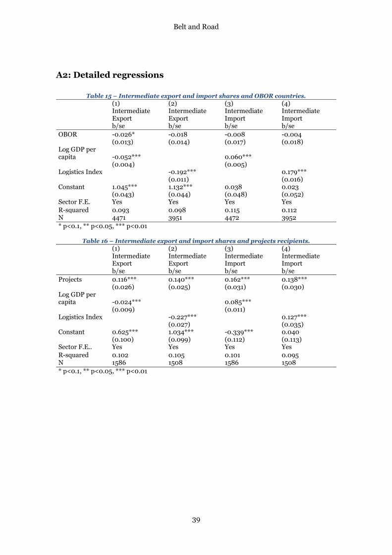
Belt and Road
39
A2: Detailed regressions
Table 15 – Intermediate export and import shares and OBOR countries.
(1) (2) (3) (4)
Intermediate Export
Intermediate Export
Intermediate Import
Intermediate Import
b/se b/se b/se b/se OBOR -0.026* -0.018 -0.008 -0.004
(0.013) (0.014) (0.017) (0.018) Log GDP per capita -0.052*** 0.060*** (0.004) (0.005) Logistics Index -0.192*** 0.179***
(0.011) (0.016) Constant 1.045*** 1.132*** 0.038 0.023
(0.043) (0.044) (0.048) (0.052) Sector F.E. Yes Yes Yes Yes R-squared 0.093 0.098 0.115 0.112 N 4471 3951 4472 3952 * p<0.1, ** p<0.05, *** p<0.01
Table 16 – Intermediate export and import shares and projects recipients.
(1) (2) (3) (4)
Intermediate Export
Intermediate Export
Intermediate Import
Intermediate Import
b/se b/se b/se b/se Projects 0.116*** 0.140*** 0.162*** 0.138***
(0.026) (0.025) (0.031) (0.030) Log GDP per capita -0.024*** 0.085***
(0.009) (0.011) Logistics Index -0.227*** 0.127***
(0.027) (0.035) Constant 0.625*** 1.034*** -0.339*** 0.040
(0.100) (0.099) (0.112) (0.113) Sector F.E.. Yes Yes Yes Yes R-squared 0.102 0.105 0.101 0.095 N 1586 1508 1586 1508 * p<0.1, ** p<0.05, *** p<0.01

Belt and Road
40
Table 17 – Intermediate trade with China and OBOR countries.
(1) (2) (3) (4)
Intermediate ExportCHN
Intermediate ExportCHN
Intermediate ImportCHN
Intermediate ImportCHN
b/se b/se b/se b/se OBOR 0.091*** 0.101*** 0.019 0.030
(0.029) (0.031) (0.021) (0.020) Log GDP per capita 0.027*** 0.040*** (0.009) (0.008) Logistics Index 0.118*** 0.199***
(0.030) (0.023) Constant -1.837*** -1.925*** -2.175*** -2.417***
(0.111) (0.130) (0.090) (0.086) Sector F.E. Yes Yes Yes Yes R-squared 0.033 0.039 0.085 0.094 N 4471 3951 4472 3952 * p<0.1, ** p<0.05, *** p<0.01
Table 18 – Intermediate trade with China and projects recipients.
(1) (2) (3) (4)
Intermediate ExportCHN
Intermediate ExportCHN
Intermediate ImportCHN
Intermediate ImportCHN
b/se b/se b/se b/se Projects 0.102* 0.168*** -0.115*** -0.113***
(0.056) (0.058) (0.030) (0.032) Log GDP per capita -0.075*** -0.105***
(0.021) (0.012) Logistics Index -0.096 0.005
(0.069) (0.043) Constant -0.797*** -1.230*** -0.691*** -1.580***
(0.229) (0.244) (0.138) (0.146) Sector F.E. Yes Yes Yes Yes R-squared 0.045 0.043 0.090 0.086 N 1586 1508 1586 1508 * p<0.1, ** p<0.05, *** p<0.01
Table 19 – Balassa RCA overlap and OBOR countries. (1) (2) (3) (4) nRCA12over~D nRCA12over~D nRCA12over~p nRCA12over~p b/se b/se b/se b/se
OBOR 0.152*** 0.141*** 0.119*** 0.108*** (0.042) (0.044) (0.017) (0.018)
Log GDP per capita 0.060***
0.076***
(0.013)
(0.005)
Logistics Index 0.198***
0.310*** (0.038)
(0.017)
Constant -1.051*** -1.169*** -0.164*** -0.407*** (0.156) (0.157) (0.055) (0.059)
Sector F.E. Yes Yes Yes Yes R-squared 0.175 0.154 0.061 0.066 N 4472 3952 4472 3952 * p<0.1, ** p<0.05, *** p<0.01
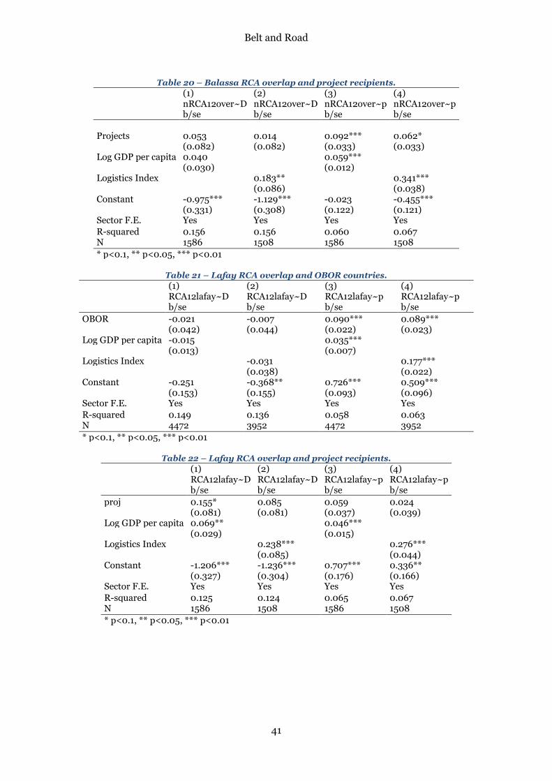
Belt and Road
41
Table 20 – Balassa RCA overlap and project recipients.
(1) (2) (3) (4)
nRCA12over~D nRCA12over~D nRCA12over~p nRCA12over~p
b/se b/se b/se b/se
Projects 0.053 0.014 0.092*** 0.062*
(0.082) (0.082) (0.033) (0.033) Log GDP per capita 0.040 0.059***
(0.030) (0.012) Logistics Index 0.183** 0.341***
(0.086) (0.038) Constant -0.975*** -1.129*** -0.023 -0.455***
(0.331) (0.308) (0.122) (0.121) Sector F.E. Yes Yes Yes Yes R-squared 0.156 0.156 0.060 0.067 N 1586 1508 1586 1508 * p<0.1, ** p<0.05, *** p<0.01
Table 21 – Lafay RCA overlap and OBOR countries.
(1) (2) (3) (4)
RCA12lafay~D RCA12lafay~D RCA12lafay~p RCA12lafay~p
b/se b/se b/se b/se OBOR -0.021 -0.007 0.090*** 0.089***
(0.042) (0.044) (0.022) (0.023) Log GDP per capita -0.015 0.035*** (0.013) (0.007) Logistics Index -0.031 0.177***
(0.038) (0.022) Constant -0.251 -0.368** 0.726*** 0.509***
(0.153) (0.155) (0.093) (0.096) Sector F.E. Yes Yes Yes Yes R-squared 0.149 0.136 0.058 0.063 N 4472 3952 4472 3952 * p<0.1, ** p<0.05, *** p<0.01
Table 22 – Lafay RCA overlap and project recipients.
(1) (2) (3) (4)
RCA12lafay~D RCA12lafay~D RCA12lafay~p RCA12lafay~p
b/se b/se b/se b/se proj 0.155* 0.085 0.059 0.024
(0.081) (0.081) (0.037) (0.039) Log GDP per capita 0.069** 0.046***
(0.029) (0.015) Logistics Index 0.238*** 0.276***
(0.085) (0.044) Constant -1.206*** -1.236*** 0.707*** 0.336**
(0.327) (0.304) (0.176) (0.166) Sector F.E. Yes Yes Yes Yes R-squared 0.125 0.124 0.065 0.067 N 1586 1508 1586 1508 * p<0.1, ** p<0.05, *** p<0.01
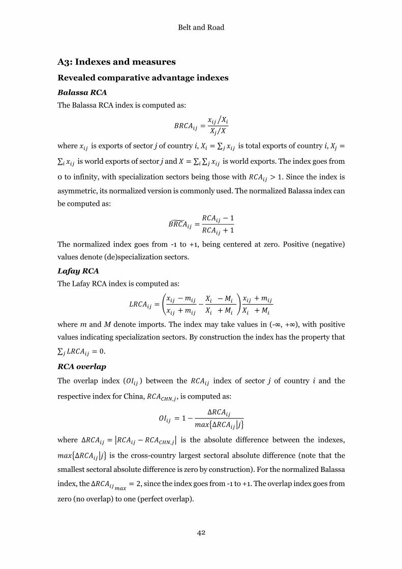
Belt and Road
42
A3: Indexes and measures
Revealed comparative advantage indexes
Balassa RCA
The Balassa RCA index is computed as:
𝐵𝑅𝐶𝐴𝑖𝑗 =𝑥𝑖𝑗 𝑋𝑖⁄
𝑋𝑗 𝑋⁄
where 𝑥𝑖𝑗 is exports of sector j of country i, 𝑋𝑖 = ∑ 𝑥𝑖𝑗𝑗 is total exports of country i, 𝑋𝑗 =
∑ 𝑥𝑖𝑗𝑖 is world exports of sector j and 𝑋 = ∑ ∑ 𝑥𝑖𝑗𝑗𝑖 is world exports. The index goes from
0 to infinity, with specialization sectors being those with 𝑅𝐶𝐴𝑖𝑗 > 1. Since the index is
asymmetric, its normalized version is commonly used. The normalized Balassa index can
be computed as:
𝐵𝑅𝐶��𝑖𝑗 =𝑅𝐶𝐴𝑖𝑗 − 1
𝑅𝐶𝐴𝑖𝑗 + 1
The normalized index goes from -1 to +1, being centered at zero. Positive (negative)
values denote (de)specialization sectors.
Lafay RCA
The Lafay RCA index is computed as:
𝐿𝑅𝐶𝐴𝑖𝑗 = (𝑥𝑖𝑗 − 𝑚𝑖𝑗
𝑥𝑖𝑗 + 𝑚𝑖𝑗
−𝑋𝑖 − 𝑀𝑖
𝑋𝑖 + 𝑀𝑖
)𝑥𝑖𝑗 + 𝑚𝑖𝑗
𝑋𝑖 + 𝑀𝑖
where m and M denote imports. The index may take values in (-∞, +∞), with positive
values indicating specialization sectors. By construction the index has the property that
∑ 𝐿𝑅𝐶𝐴𝑖𝑗𝑗 = 0.
RCA overlap
The overlap index (𝑂𝐼𝑖𝑗 ) between the 𝑅𝐶𝐴𝑖𝑗 index of sector j of country i and the
respective index for China, 𝑅𝐶𝐴𝐶𝐻𝑁,𝑗, is computed as:
𝑂𝐼𝑖𝑗 = 1 −∆𝑅𝐶𝐴𝑖𝑗
𝑚𝑎𝑥{∆𝑅𝐶𝐴𝑖𝑗 |𝑗}
where ∆𝑅𝐶𝐴𝑖𝑗 = |𝑅𝐶𝐴𝑖𝑗 − 𝑅𝐶𝐴𝐶𝐻𝑁,𝑗| is the absolute difference between the indexes,
𝑚𝑎𝑥{∆𝑅𝐶𝐴𝑖𝑗|𝑗} is the cross-country largest sectoral absolute difference (note that the
smallest sectoral absolute difference is zero by construction). For the normalized Balassa
index, the ∆𝑅𝐶𝐴𝑖𝑗 𝑚𝑎𝑥= 2, since the index goes from -1 to +1. The overlap index goes from
zero (no overlap) to one (perfect overlap).
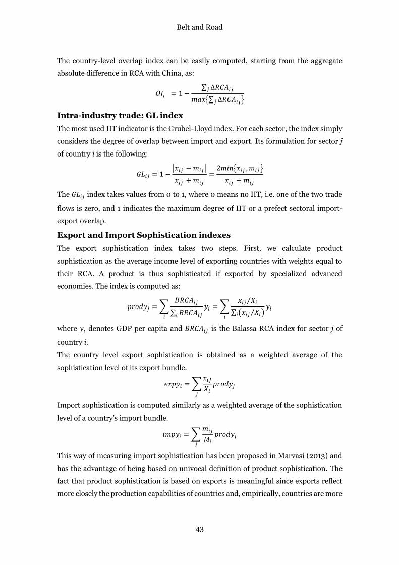
Belt and Road
43
The country-level overlap index can be easily computed, starting from the aggregate
absolute difference in RCA with China, as:
𝑂𝐼𝑖 = 1 −∑ ∆𝑅𝐶𝐴𝑖𝑗𝑗
𝑚𝑎𝑥{∑ ∆𝑅𝐶𝐴𝑖𝑗𝑗 }
Intra-industry trade: GL index
The most used IIT indicator is the Grubel-Lloyd index. For each sector, the index simply
considers the degree of overlap between import and export. Its formulation for sector j
of country i is the following:
𝐺𝐿𝑖𝑗 = 1 −|𝑥𝑖𝑗 − 𝑚𝑖𝑗 |
𝑥𝑖𝑗 + 𝑚𝑖𝑗
=2𝑚𝑖𝑛{𝑥𝑖𝑗 , 𝑚𝑖𝑗 }
𝑥𝑖𝑗 + 𝑚𝑖𝑗
The 𝐺𝐿𝑖𝑗 index takes values from 0 to 1, where 0 means no IIT, i.e. one of the two trade
flows is zero, and 1 indicates the maximum degree of IIT or a prefect sectoral import-
export overlap.
Export and Import Sophistication indexes
The export sophistication index takes two steps. First, we calculate product
sophistication as the average income level of exporting countries with weights equal to
their RCA. A product is thus sophisticated if exported by specialized advanced
economies. The index is computed as:
𝑝𝑟𝑜𝑑𝑦𝑗 = ∑𝐵𝑅𝐶𝐴𝑖𝑗
∑ 𝐵𝑅𝐶𝐴𝑖𝑗𝑖
𝑦𝑖
𝑖
= ∑𝑥𝑖𝑗 𝑋𝑖⁄
∑ (𝑥𝑖𝑗 𝑋𝑖⁄ )𝑖
𝑦𝑖
𝑖
where 𝑦𝑖 denotes GDP per capita and 𝐵𝑅𝐶𝐴𝑖𝑗 is the Balassa RCA index for sector j of
country i.
The country level export sophistication is obtained as a weighted average of the
sophistication level of its export bundle.
𝑒𝑥𝑝𝑦𝑖 = ∑𝑥𝑖𝑗
𝑋𝑖𝑝𝑟𝑜𝑑𝑦𝑗
𝑗
Import sophistication is computed similarly as a weighted average of the sophistication
level of a country’s import bundle.
𝑖𝑚𝑝𝑦𝑖 = ∑𝑚𝑖𝑗
𝑀𝑖𝑝𝑟𝑜𝑑𝑦𝑗
𝑗
This way of measuring import sophistication has been proposed in Marvasi (2013) and
has the advantage of being based on univocal definition of product sophistication. The
fact that product sophistication is based on exports is meaningful since exports reflect
more closely the production capabilities of countries and, empirically, countries are more

Belt and Road
44
diverse in their export bundles than in their import bundles. The implication of
measuring import sophistication in this way is that countries with sophisticated imports
are those that buy sophisticated products, that is products that tend to be exported by
richer countries. This is particularly useful when input-output linkages matter, since
import sophistication is likely to capture the fact that a country obtains its inputs from
advanced economies, a fact that may represent itself a source of competitive advantage
in GVC.
Figure 15 – Export and import sophistication.
Source: authors’ elaborations based on Eora and WDI.
99
.29
.49
.69
.8
6 7 8 9 10 11 12Log GDP per capita 2012
95% CI predicted ln_expy12
ln_expy12 predicted ln_impy12
ln_impy12

Belt and Road
45
A4: Network centrality indicators
Table 23 – Centrality in the OBOR intermediate trade network (manufacturing; trade weighted indicators)
PageRank Hubs Authorities Outdegree Indegree Betweenness China 0,148 0,112 0,258 18,0 21,3 3025 Singapore 0,080 0,170 0,175 13,0 13,4 427 Russia 0,072 0,114 0,015 11,1 5,5 1900 India 0,066 0,052 0,062 6,0 6,4 1160 Malaysia 0,048 0,177 0,097 10,4 7,1 0 Thailand 0,043 0,074 0,074 4,7 5,6 122 Turkey 0,034 0,007 0,020 1,8 3,0 262 Ukraine 0,030 0,007 0,029 2,7 3,4 61 Czech Republic 0,027 0,010 0,011 3,6 2,6 120 Poland 0,027 0,005 0,016 2,2 2,9 44 Saudi Arabia 0,025 0,014 0,013 1,4 2,0 122 UAE 0,024 0,009 0,016 1,7 2,0 272 Indonesia 0,024 0,117 0,047 7,1 3,2 0 Iran 0,023 0,011 0,009 1,0 1,4 121 Hungary 0,022 0,005 0,013 1,6 2,1 288
Source: authors’ elaborations based on Eora.
Table 24 – Correlation of centrality indicators of the OBOR intermediate trade network (manufacturing; trade weighted indicators)
PageRank Hubs Authorities Outdegree Indegree Betweenness PageRank 1 Hubs 0,755 1 Authorities 0,907 0,782 1 Outdegree 0,945 0,908 0,905 1 Indegree 0,972 0,780 0,977 0,946 1 Betweenness 0,872 0,502 0,703 0,779 0,797 1
Source: authors’ elaborations based on Eora.
Table 25 – Rank correlation of centrality indicators of the OBOR intermediate trade network (manufacturing; trade weighted indicators)
PageRank Hubs Authorities Outdegree Indegree Betweenness PageRank 1 Hubs 0,769 1 Authorities 0,869 0,852 1 Outdegree 0,883 0,914 0,848 1 Indegree 0,964 0,814 0,938 0,896 1 Betweenness 0,591 0,501 0,471 0,572 0,531 1
Source: authors’ elaborations based on Eora.