Global Real Rates: A Secular Approach∗

Pierre-Olivier GourinchasUniversity of California at Berkeley , NBER, CEPR

Helene ReyLondon Business School, NBER, CEPR

PreliminaryThis Version: April 20, 2017

Abstract

The current environment is characterized by low real rates and by policy rates close to orat their effective lower bound in all major financial areas. We analyze these unusual economicconditions from a secular perspective using data on aggregate consumption, wealth and assetreturns. Our present-value approach decomposes fluctuations in the global consumption-to-wealth ratio over long periods of time and show that this ratio anticipates future movementsof the global real rate of interest. Our analysis identifies two historical episodes where theconsumption-to-wealth ratio declined rapidly below its historical average: in the late 1920sand again in the mid 2000s. Each episode was followed by a severe global financial crisis anddepressed real rates for an extended period of time. Our empirical estimates suggest that theworld real rate of interest is likely to remain low or negative for an extended period of time.

∗Nick Sander provided outstanding research assistance. We thank Ricardo Caballero, Emmanuel Farhi, MartinLettau and Gabriel Zucman for comments. All errors remain our own. Special thanks to Oscar Jorda, MoritzSchularick and Alan Taylor for sharing their data with us. Contact email: pog@berkeley.edu.

1 Introduction

The current macroeconomic environment remains a serious source of worry for policymakers and of

puzzlement for academic economists. Global real rates have been trending down since the 1980s are

at historical lows across advanced economies, both at the short and long end of the term structure.

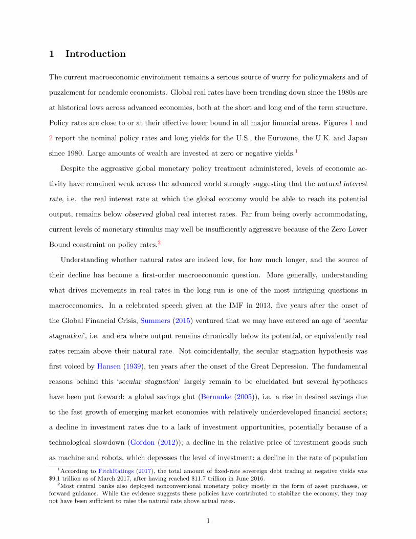
Policy rates are close to or at their effective lower bound in all major financial areas. Figures 1 and

2 report the nominal policy rates and long yields for the U.S., the Eurozone, the U.K. and Japan

since 1980. Large amounts of wealth are invested at zero or negative yields.1

Despite the aggressive global monetary policy treatment administered, levels of economic ac-

tivity have remained weak across the advanced world strongly suggesting that the natural interest

rate, i.e. the real interest rate at which the global economy would be able to reach its potential

output, remains below observed global real interest rates. Far from being overly accommodating,

current levels of monetary stimulus may well be insufficiently aggressive because of the Zero Lower

Bound constraint on policy rates.2

Understanding whether natural rates are indeed low, for how much longer, and the source of

their decline has become a first-order macroeconomic question. More generally, understanding

what drives movements in real rates in the long run is one of the most intriguing questions in

macroeconomics. In a celebrated speech given at the IMF in 2013, five years after the onset of

the Global Financial Crisis, Summers (2015) ventured that we may have entered an age of ‘secular

stagnation’, i.e. and era where output remains chronically below its potential, or equivalently real

rates remain above their natural rate. Not coincidentally, the secular stagnation hypothesis was

first voiced by Hansen (1939), ten years after the onset of the Great Depression. The fundamental

reasons behind this ‘secular stagnation’ largely remain to be elucidated but several hypotheses

have been put forward: a global savings glut (Bernanke (2005)), i.e. a rise in desired savings due

to the fast growth of emerging market economies with relatively underdeveloped financial sectors;

a decline in investment rates due to a lack of investment opportunities, potentially because of a

technological slowdown (Gordon (2012)); a decline in the relative price of investment goods such

as machine and robots, which depresses the level of investment; a decline in the rate of population

1According to FitchRatings (2017), the total amount of fixed-rate sovereign debt trading at negative yields was$9.1 trillion as of March 2017, after having reached $11.7 trillion in June 2016.

2Most central banks also deployed nonconventional monetary policy mostly in the form of asset purchases, orforward guidance. While the evidence suggests these policies have contributed to stabilize the economy, they maynot have been sufficient to raise the natural rate above actual rates.

1

-5

0

5

10

15

20

25

1980 1983 1986 1989 1992 1995 1998 2001 2004 2007 2010 2013 2016

percent

U.S. Eurozone U.K. Japan

Financial Crisis Eurozone Crisis

Figure 1: Policy Rates, 1980-2016. Sources: U.S.: Federal Funds Official Target Rate; Eurozone:

until Dec. 1998, Germany’s Lombard Rate. After 1998, ECB Marginal Rate of Refinancing Operations;

U.K.: Bank of England Base Lending Rate; Japan: Bank of Japan Target Call Rate. Data from Global

Financial Database.

-2

0

2

4

6

8

10

12

14

16

18

1980 1983 1986 1989 1992 1995 1998 2001 2004 2007 2010 2013 2016

percent

U.S. Germany U.K. Japan

Financial Crisis Eurozone Crisis

Figure 2: Long yields. 1980-2016. Sources: U.S.: 10-year bond constant maturity rate; Germany:

10-year benchmark bond; U.K.: 10-year government bond yield; Japan: 10-year government bond yield.

Data from Global Financial Database

2

growth; an increase in the demand for safe assets (Caballero et al. (2015)).

This paper is an empirical contribution to this debate. Using an almost a-theoretical empirical

approach inspired by the finance literature but applied to long run historical data, we show that

low-frequency movements in the consumption-to-wealth ratio are key to understand movements

in the global real interest rate. We find that, as in other historical periods, most notably in the

1930s, low real rates are the likely outcome of an extended and on-going process of deleveraging

that creates a ‘scarcity of safe assets.’ As a by product of our analysis, we are also able to make

some low frequency forecasts of the real rate.

1.1 Review of the Literature

This is a placeholder for a literature review. It will include:

• papers on estimation of the natural rate: Laubach and Williams (2016, 2003); Hamilton et al.

(2015); Pescatori and Turunen (2015); Del Negro et al. (2017); Farooqui (2016); Barro and

Sala-i Martin (1990)

• papers on secular stagnation: Eggertsson et al. (2015); Eggertsson and Mehrotra (2014);

Caballero et al. (2015); Summers (2015); Hansen (1939); Sajedi and Thwaites (2016)

• papers on the present value approach: Campbell and Shiller (1991); Lettau and Ludvigson

(2001); Gourinchas and Rey (2007)

2 Dynamics of Global Real Interest rates

This section, presents a present value model that connects low frequency movements in aggregate

consumption, wealth and asset returns.

2.1 The Global Budget Constraint: Some Elements of Theory

We are interested in understanding the determinants of the global safe real interest rate. With

integrated capital markets, the relevant unit of analysis is the global (i.e. world) resource constraint.

Denote the beginning-of-period global total private wealth Wt, composed of global private wealth

3

Wt and global human wealth Ht.3 Total private wealth evolves over time according to:

Wt+1 = Rt+1(Wt − Ct). (1)

In equation (1), Ct denotes global private consumption expenditures and Rt+1 the gross return

on total private wealth between periods t and t + 1.4 All variables are expressed in real terms.

Equation (1) is simply an accounting identity that holds period-by-period. We add some structure

to this identity by observing that, in most theoretical models, households aim to smooth consump-

tion and stabilize the consumption-to-wealth ratio.5 If the average propensity to consume out of

wealth is stationary, equation (1) can be log-linearized around its steady state value C/W ≡ 1−ρw,

where ρw < 1.6 Denote ∆ the difference operator so that ∆xt+1 ≡ xt+1 − xt, and rt+1 ≡ ln Rt+1,

the continuously compounded real return on wealth. Following the same steps as Campbell and

Mankiw (1989) or Lettau and Ludvigson (2001), we obtain the following log-linearized expression

(ignoring an unimportant constant term) :7

lnCt − ln Wt w ρw(lnCt+1 − ln Wt+1 + rt+1 −∆ lnCt+1

). (2)

Equation (2) indicates that if today’s consumption-to-wealth ratio is high, then either (a) to-

morrow’s consumption-to-wealth ratio will be high, or (b) the return on wealth between today

and tomorrow rt+1 will be high, or (c) aggregate consumption growth ∆ lnCt+1 will be low. Since

ρw < 1, Equation (2) can be iterated forward to obtain, under the usual transversality condition

(limj→∞ Etρjwcwt+j = 0 ), the following ex-ante present value relation:

lnCt − ln Wt w Et∞∑s=1

ρsw (rt+s −∆ lnCt+s) . (3)

3Private wealth includes financial assets, including private holdings of government assets, as well as non-financialassets, but excludes human wealth. See the appendix for a detailed data description.

4We focus on total private wealth and consumption, and not total national wealth or consumption, which includesgovernment’s net wealth and consumption. This is the appropriate focus under the -reasonable- assumption thatRicardian equivalance fails.

5For instance, if consumption decisions are taken by an infinitely lived representative household maximizing welfaredefined as the expected present value of a logarithmic period utility u(C) = lnC, then the consumption-to-wealthratio is constant and equal to the discount rate of the representative agent.

6In steady state, C/W satisfies the following relation: Γ/R = 1 − C/W ≡ ρw, where Γ denotes the steady stategrowth rate of total private wealth and R the steady state gross return on wealth.

7See the appendix for a full derivation.

4

To understand equation (3), suppose that the consumption-to-wealth ratio (the left hand side

of the equation) is currently higher than its unconditional mean. Since C/W is stationary, this

ratio must be expected to decline in the future. Equation (3) states that this decline can occur in

one of two ways. First, expected future return on total private wealth rt+s could be high. This

would increase future wealth, i.e. the denominator of the C/W ratio. Alternatively expected future

aggregate consumption growth could be low, which would decrease the numerator of C/W .

At this stage, it is important to emphasize that the assumptions needed to derive equation (3)

are very minimal: we start from the law of motion of total private wealth, equation (1), which

is an accounting identity. We then perform a log-linearization under mild stationarity conditions,

and impose a transversality condition that rules out paths where wealth grows without bounds in

relation to consumption. Equation (3)’s main economic message is that today’s average propensity

to consume out of wealth encodes relevant information about future consumption growth and/or

future returns to wealth.

Before we can exploit this expression empirically, we need to make two important adjustments.

First, as mentioned above, total private wealth is the sum of private wealth Wt and human wealth

Ht. Because human wealth is not easily observable, Lettau and Ludvigson (2001) approximate

the non-stationary component of human wealth with aggregate labor income and estimate a co-

integration relation between consumption, financial wealth and labor income to construct a proxy

for the left hand side of equation (3).8 We follow a different route. Specifically, denote ω the

aggregate share of private wealth in total wealth: ω = W/W . If ω is stationary, we can approximate

(log) total wealth as ln Wt = ω lnWt + (1 − ω) lnHt, and the log return on total wealth as rt =

ωrwt +(1−ω)rht where rwt (resp. rht ) denotes the log return on private wealth (resp. human wealth).9

Substituting these expressions into equation (3) and re-arranging we obtain:

ω

(lnCt − lnWt − Et

∞∑s=1

ρsw(rwt+s −∆ lnCt+s

))+(1−ω)

(lnCt − lnHt − Et

∞∑s=1

ρsw

(rht+s −∆ lnCt+s

))w 0.

(4)

This equation makes clear that if the present value relation holds for private wealth, then it

8Lettau and Ludvigson (2001) also use a co-integration approach since the ratio C/W does not appear stationaryin their shorter sample.

9The gross return on human wealth may be defined as Rht+1 = exp(rht+1

)= (Ht+1 + WLt+1)/Ht where WLt+1

denotes the aggregate compensation of capital in period t+ 1. See Campbell (1996).

5

holds for human wealth, and vice versa. More generally, we can write:

lnCt − lnWt w Et∞∑s=1

ρsw(rwt+s −∆ lnCt+s

)+ εt. (5)

where εt represents the error term induced by ignoring human wealth.10

The second step is to realize that the return on private wealth rwt can always be decomposed

into the sum of a real risk free rate rft and a risk premium rpwt according to: rwt = rft + rpwt . While

we can construct reasonably accurate estimates of the real risk free rate rft , we do not observe the

risk premium on private wealth rpwt (or equivalently, the return to private wealth). This is so since

private wealth includes a variety of financial assets such as portfolio holdings whose return could

reasonably be approximated, but includes also non-financial assets such as housing, agricultural land

and equipments whose returns are more difficult to measure. Our approach consists in proxying

the return on private wealth by assuming that :

rwt = rft + ν rpt, (6)

where rpt is the observed excess global equity return, and ν is an adjustment parameter that will

be estimated in order to maximize the empirical fit of equation (5).11

10From equation (4) and with some simple manipulations, we can write :

εt = (1 − ω)

(Et∞∑s=1

ρsw

(rht+s − rwt+s

)− (lnWt − lnHt)

)

This error term is small when expected returns on human and private wealth are similar, and when the ratioof private to human wealth is stationary. Accordingly, the consumption-to-private wealth ratio may be low whenexpected future returns to human wealth are low relative to the returns on private wealth, or when human wealth islow relative to private financial wealth. The recent evidence on the decline in the labor share (see e.g. Karabarbounisand Neiman (2014)) and on the increase in income ineqality (see e.g. Piketty and Saez (2003)) could invalidate theseassumptions. However, our focus on long run data should mitigate these concerns. For instance, as documentedby Piketty and Saez (2003), the dynamics of income inequality over the last century is characterized by large andpersistent fluctuations, but no historical trend: income inequality in the U.S. is today close to what it was at thebeginning of the XXth century. Over shorter horizons, as in Lettau and Ludvigson (2001), the consumption-to-wealthratio may appear non-stationary.

11Specifically we estimate ν via OLS so as to minimize the residuals in equation (5). This opens up the possibilitythat the risk premium component may be contaminated by the human capital component. Specifically, the OLSestimate of ν satisfies ν = ν + cov (ε, cwrp)/var(cwrp) where cwrp = Et

∑∞s=1 ρ

sw rpt+s is the estimated present value

of future global equity risk premia. The possible bias on ν attributes to the risk premium component the part of thevariation in lnC− lnW that should be attributed to fluctuations in human wealth and co-moves with the equity riskpremium.

6

Substituting (6) into the present value relation (5), we obtain our fundamental representation:

lnCt − lnWt w Et∞∑s=1

ρswrft+s + νEt

∞∑s=1

ρswrpt+s − Et∞∑s=1

ρsw∆ lnCt+s + εt. (7)

≡ cwft + cwrpt + cwct + εt.

This equation states that the ratio of aggregate consumption to private wealth should contain

information either about (a) future safe rates rft+s, (b) future excess returns rpt+s, or (c) future

aggregate consumption growth ∆ lnCt+s. The terms cwft , cwrpt and cwct summarize the relative

contributions of the risk free rate, the risk premia and consumption growth. Inspecting (7), it

is well-known that aggregate consumption is close to a random walk, and that the risk premium

is volatile and difficult to predict. Therefore, if anything we expect equation (7) to connect the

aggregate consumption-to-wealth ratio and the expected path of future real risk free returns rft+s.

2.2 Interpretation

Before we lay out our empirical strategy, we discuss how different fundamental shocks can affect

returns, consumption and the consumption/wealth ratio.

2.2.1 Productivity shocks and consumption smoothing

As discussed, equation (7) does not provide a causal decomposition: the risk free, risk premium

and consumption growth components are both endogenous and interdependent. To see this more

clearly, let’s consider a closed endowment economy with no government, so consumption C is equal

to output Y . Equation (7) takes the form:

lnCt − lnWt w Et∞∑s=1

ρsw(rwt+s −∆ lnYt+s

). (8)

Suppose that total output growth is expected to decline. According to equation (8), for a

given expected path of future returns, this should increase the consumption wealth ratio. However,

expected future returns will not remain constant. Faced with a future slowdown in output growth,

today’s households may want to save more. In equilibrium, this will depress expected future

returns, up to the point where consumption growth equals output growth. In turn, the decline in

7

returns will exert downward pressure on the consumption-to-wealth ratio. To see this mechanism

more explicitly, assume that the representative household has additively separable preferences over

consumption, with a constant intertemporal elasticity of substitution (IES) 1/σ and a discount rate

ρ. The usual log-linearized Euler equation takes the following form (up to the second order):

σEt∆ lnCt+1 = Etrwt+1 − ρ+1

2σ2z,t,

where σ2z,t denotes the conditional variance of zt+1 = rwt+1 − σ∆ lnCt+1 at time t.

Denote gt = ∆ lnYt = ∆ lnCt the (exogenous) aggregate growth rate of output, and σ2g,t its

conditional variance. In equilibrium, the Euler equation expresses the expected return on wealth

as :

Etrwt+1 = ρ+ σEtgt+1 −1

2σ2z,t. (9)

This expression encodes precisely the extent to which the return on wealth needs to respond to

changes in expected output growth so as to clear the goods market: if output growth is expected

to increase by 1%, the expected return on private wealth must increase by σ%. Substituting the

Euler equation (9) into equation (8) one obtains:

lnCt − lnWt w Et∞∑s=1

ρsw

((σ − 1)gt+s + ρ− 1

2σ2z,t+s

). (10)

It is immediate from equation (10) that whether the consumption-to-wealth ratio increases or

decreases with output growth depends on the sign of σ − 1, i.e. on the relative strength of the

substitution and income effects. If σ > 1, the IES is low and interest rates need to decline a

lot in order to stimulate consumption growth when productivity growth declines. The impact of

productivity changes on interest rates dominates and C/W comoves positively with expected future

productivity growth. If instead σ < 1, the IES is high and a modest decline in real interest rates is

sufficient to push consumption growth down. The direct impact of productivity growth dominates

and C/W comoves negatively with expected future productivity growth.12

Following similar steps, one can compute the various components cwit as (up to some unimpor-

12In the special case where σ = 1, the consumption-wealth ratio is constant independent from Etgt+s.

8

tant constants):

cwft = σEt∞∑s=1

ρsw

(gt+s −

σ

2σ2g,t+s

)cwrpt = Et

∞∑s=1

ρsw

(σcovt(r

wt+s, gt+s)−

1

2σ2r,t+s

)

cwct = −Et∞∑s=1

ρswgt+s,

where σ2r,t is the conditional variance of the return on private wealth.

These expressions make clear that expected changes in productivity growth have direct opposite

effects on the risk free and consumption components, scaled by the IES. This is most evident if

there is no time-variation in second moments, in which case the risk premium component is constant

while the risk free and consumption components are perfectly negatively correlated.13

2.2.2 Demographics

Consider now the effect of demographic forces on the consumption-to-wealth ratio. To do so,

decompose total consumption growth ∆ lnCt+1 into per capita consumption growth ∆ ln ct+1, and

population growth nt+1: ∆ lnCt+1 = ∆ ln ct+1 + nt+1. Substituting into (5) we obtain:

ln ct − lnwt w Et∞∑s=1

ρsw(rwt+s −∆ ln ct+s − nt+s

),

where wt denotes real private wealth per capita. It is obvious from this expression that an expected

decline in population growth (Etnt+s < 0) has a direct and positive effect on c−w, given a path of

returns and consumption per capita. The effect of a decline in population growth on equilibrium

interest rates, and therefore the indirect effect on the consumption-to-weath ratio, is more complex.

As population growth slows down, this reduces the marginal product of capital, pushing down rw.

Aging, by increasing life expectancy, also leads to increased saving and therefore a decline in interest

rates. On the other hand, a lower population growth increases the dependency ratio (i.e. the ratio

of retirees to working age population). This tends to reduce aggregate savings, pushing interest

13Of course, risk premia may not be constant. For most models of interest, however, the correlation between returnson wealth and consumption growth is relatively small, indicating a small role for the macroeconomic risk premiumthat we measure here.

9

rates up (see Carvalho et al. (2016) for a discussion of the various channels). The empirical evidence

as well as calibrated overlapping generation models generally indicate that slowdowns in population

growth are associated with increased savings.14 This should push down the consumption-to-wealth

ratio with the strength of that effect, again, controlled by the intertemporal elasticity of substitution

1/σ. In this case, as in the case of productivity shocks, the impact of demographic shocks will

have opposite effects on the risk free and consumption growth components: corr(cwft , cwct ) < 0.

Importantly, we can measure the direct effect of demographic shocks on the consumption-to-wealth

ratio by constructing cwnt = −Et∑∞

s=1 ρswnt+s. If demographic forces are an important driver of

wealth and consumption movements, we expect that cwn and cwf be negatively correlated.

2.2.3 Deleveraging shock

Consider next what happens if there is a sudden shift in individuals’ desire to save. At an abstract

level, one can model this shift as a decrease in ρ, the discount rate of households. Such deleveraging

shocks have been studied by Eggertsson and Krugman (2012), as well as Guerrieri and Lorenzoni

(2011). To understand how these shocks may affect the consumption-to-wealth ratio, we need to

consider two cases, depending on whether the economy is above or at the effective lower bound

(ELB).

Consider first the case where the economy is above the ELB. For simplicity, assume that output

is constant. With consumption equal to output in equilibrium, the Euler equation becomes

Etrwt+1 = ρt+1 −1

2σ2r,t, (11)

where ρt+1 is the now time-varying discount rate of the representative household between periods t

and t+1, known at time t. A decline in ρt+1 pushes down the equilibrium real return on assets and,

under the assumption that the economy remains permanently above the ELB, the present-value

equation (10) becomes:

lnCt − lnWt = Et∞∑s=1

ρsw(ρt+s −1

2σ2r,t+s).

14With open economies, the same phenomenon manifests itself in the form of current account surpluses for countries,such as Japan, Germany and China, with rapid slowdown in population growth and aging.

10

We can express the different components as:

cwft = Et∞∑s=1

ρswρt+s

cwrpt = −1

2Et∞∑s=1

ρswσ2r,t+s

cwct = 0.

An expected deleveraging shock, i.e. a decline in Etρt+s, has a direct negative effect on the

consumption-to-wealth ratio because it lowers the real risk free rate one for one, but no effect

on the consumption or risk premia components.

Consider now what happens at the ELB. If prices are nominally rigid and nominal interest rates

cannot decrease further to satisfy (11), the economy will experience a recession, as in Eggertsson

and Krugman (2012) or Caballero and Farhi (2015). For simplicity, suppose that the effective lower

bound is zero and that prices are permanently fixed so that rf = 0 while the economy remains at

the ELB. The Euler equation requires that:

σEt∆ lnCt+1 = −ρt+1 +σ2

2vart (σ∆ lnCt+1) .

Consumption is expected to increase at a rate that reflects the (positive) gap between the real

interest rate and the natural real interest rate. Since potential output is constant this expression

makes clear that the economy must experience a recession today (i.e. output and consumption

need to be below potential). The expected return on wealth (equal to the expected excess return)

now satisfies:

Etrwt+1 = covt(rwt+1, σ∆ lnCt+1)−

1

2σ2r,t,

and may change as the economy hits the ELB, as emphasized by Caballero et al. (2016). If

the economy is expected to remain permanently at the ELB, the different components of the

11

consumption-to-wealth ratio can be expressed as:

cwft = 0

cwrpt = Et∞∑s=1

ρsw

(covt(r

wt+s, σ lnCt+s)−

1

2σ2r,t+s

)

cwct =1

σEt∞∑s=1

ρsw

(ρt+1 −

σ2

2vart (∆ lnCt+1)

).

This expression makes clear that at the ELB, the adjustment in the consumption-to-wealth

ratio occurs through the consumption component. In the general case where the economy does not

remain stuck at the ELB permanently, the adjustment will occur both via a decline in the real risk

free rate -when the economy is expected to leave the ELB– and via an increase in consumption

growth –while the economy is at the ELB. Both terms depress the consumption-to-wealth ratio, so

cwf and cwc will be positively correlated.

2.2.4 Demand for safe asset.

A deleveraging shock increases the demand for savings and therefore depresses the returns on all

assets. Let’s now consider a shock to risk appetite, i.e. shift in the demand for safe versus risky

assets. An easy way to capture such a shift would be an increase in the risk aversion coefficient

σ. However, as is well known, σ also plays the role of the inverse of the intertemporal elasticity of

substitution. In order to isolate the effect of a shift in risk appetite, assume that the representative

household has the following Epstein-Zin recursive preferences :

Ut =

{(1− β)C1−σ

t + β(EtU1−γt

t+1

) 1−σ1−γt

} 11−σ

,

where γt is the now time-varying coefficient of relative risk aversion and lnβ = −ρ. We maintain

a constant IES of 1/σ. Given these preferences, the risk-free rate satisfies:

rft+1 = ρ+ σEt∆ lnCt+1 +θt − 1

2σ2r,t −

θtσ2

2σ2g,t

where θt ≡ (1− γt)/(1− σ). When θt = 1, this formula collapses to the CRRA case. By contrast,

when θ 6= 1, the risk free rate depends on the variance of the market return. Standard derivations

12

provide the following expression for the expected risk premium:

Etrwt+1 − rft+1 = θtσcovt(r

wt+1, gt+1) + (1− θt)σ2r,t.

To highlight the role of fluctuations in risk appetite, consider an environment where output is

constant, so σ2g,t = 0. It follows that the consumption-to-wealth ratio can be expressed as (up to

some constant):

lnCt − ln Wt =1

2Et∞∑s=1

ρsw (1− θt+s)σ2r,t+s.

A persistent increase in risk aversion Etγt+s lowers Etθt+s and leads to an increase in the

consumption-to-wealth ratio. This is intuitive: while consumption is unchanged (and equal to

output), the decline in risk appetite lowers the current value of wealth. The decomposition (7)

yields :

cwft = −1

2Et∞∑s=1

ρsw (1− θt+s)σ2r,t+s

cwrpt = Et∞∑s=1

ρsw(1− θt+s)σ2r,t+s

cwct = 0.

An expected increase in future risk aversion increases the risk premium component cwrp and

decreases the risk free rate component cwf . The consumption component remains unchanged. This

is also intuitive: the decline in risk appetite requires an increase in risk premia. This increase in

risk premia is achieved via an increase in the expected return on risky assets and a decline in the

risk free rate. Overall, the increase in risk premia dominates (it is twice as large as the risk free

component).

2.3 Summary.

The preceding discussion highlights that, while the decomposition (7) does not provide a causal

interpretation of the different components, the co-movements of the different components offers a

natural signature about the various economic forces at play: If the consumption and risk free rate

components are negatively correlated, we would conclude that productivity and/or demographic

13

shocks play an important role. If instead the consumption and risk free rate components are either

poorly correlated or positively correlated, then we would conclude that deleveraging shocks are

likely to be more relevant. Finally, if we find that the risk free and risk premium components are

negatively correlated, we would infer that shocks to the demand for safe assets are an important

part of the story.

3 Estimating the Present Value Decomposition

We implement our empirical strategy in three steps. First, we construct estimates of the consumption-

to-wealth ratio over long periods of time. Next, we evaluate the empirical validity of equation (7)

by constructing the empirical counterparts on the right hand side of that equation and testing

whether they capture movements in the consumption-to-wealth ratio. Lastly, we investigate the

role of various drivers of the consumption-to-wealth ratio.

3.1 Data description

We use historical data on private wealth, population and private consumption for the period 1871-

2011 for the United States, the United Kingdom, Germany and France from Piketty and Zucman

(2014a) and Jorda et al. (2016) to construct measures of real per capita consumption and (beginning

of period) private wealth, expressed in constant 2010 US dollars. The top panel of Figure 3 reports

real per capita private wealth and consumption for the United States between 1871 and 2011. As

expected, historical time series on consumption and financial wealth show a long term positive trend.

U.S. real per capita consumption increased from $2,830 in 2010 dollars in 1871 to $33,793 in 2011,

while real per capita private wealth increased over the same period from $12,584 to $169,668. The

middle panel reports the consumption-to-wealth ratio. It appears relatively stable over this long

period of time, with a mean of 20.94 percent, slightly decreasing from 22.41 percent in 1871 to 19.91

percent in 2011. While the consumption-to-wealth ratio is strongly autocorrelated, formal tests of

a unit root do not find conclusive evidence of a unit root.15 We observe two periods during which

the consumption-to- wealth ratio was significantly depressed: the first one spans the 1930s, starting

shortly before the Great Depression and ending at the beginning of the 1940s. Interestingly, in 1939

15For instance, the ADF test with intercept and trend reports a value of -3.088, with a p-value of 0.113, while asimilar Phillips-Perron test reports a value of -3.23 with a p-value of 0.0824.

14

Professor Alvin Hansen writes his celebrated piece about ‘secular stagnation’ (Hansen (1939)). The

second episode of low consumption-to-wealth ratio starts around 1995 with a pronounced downward

peak in 2008. The consumption-to-wealth ratio rebounds after 2008 – largely as a result in the

decline in private wealth– back to its long run average. Perhaps not coincidentally, in the Fall

2013 at a conference at the International Monetary Fund, Larry Summers, professor at Harvard

resuscitates the idea of secular stagnation, an idea which is still haunting us in 2017 (Summers

(2015)).

The top panel of Figure 4 reports real consumption and wealth per capita for an aggregate

of the U.S., the U.K., Germany and France since 1920. We label this aggregate the ‘G-4’. Over

the period considered, these four countries represent a sizable share of the world’s financial wealth

and consumption. London, New-York, and to a lesser extent Frankfurt, represent major financial

centers. As for the U.S., real consumption and wealth per capita for the G-4 show a long term

positive trend with a few major declines during the two World Wars and the Great Depression.16

Real per capita consumption increased from $3,742 in 1920 to $26,967 in 2010 constant dollars

while real per capita private wealth increased from $19,952 to $150,680 over the same period. The

consumption-to-wealth ratio exhibits the same pattern as that of the U.S., with a mean of 20.71

percent.17

The bottom panel of figures 3 and 4 report the real risk free rate for the U.S. and for the G4

aggregate. The real risk free rate is constructed as the interest rate on 3-month Treasuries from

Jorda et al. (2016), deflated by the realized CPI inflation rate.18 Both figures document the decline

in global real interest rates since the early 1980s, from 9.6 percent in 1981 to -1.8 percent in 2011.

They also illustrate that the early 1980s may have been a relatively exceptional period: US real

16The effect of the wars on the financial wealth and consumption of Germany and France is the most dramatic.The U.S. consumption-to-wealth ratio is somewhat insulated from the shock of the wars and it does not show swingsof the amplitude of the U.K., French and German consumption wealth ratios at the time of the first world war.This, and concerns about data quality prior to 1920 are the two reasons we only begin the ‘G4’ aggregate after 1920.In particular, as discussed in the appendix, wealth data is not available annually before 1954 for France, 1950 forGermany, 1920 for the U.K. and 1916 for the U.S. and is imputed based on savings data and estimates of the rate ofcapital gains on wealth for each country.

17We are unable to reject the null of a unit root in lnC − lnW for the G4 aggregate at conventional levels ofsignificance: the ADF test with trend and intercept reports a value of -2.43 with a p-value of 0.358 while the Phillipsand Perron test reports a value of -19.3 with a p-value of 0.63. Nevertheless, we consider that this reflects the lowpower of unit root tests rather than definite evidence that the consumption-to-wealth ratio is non-stationary.

18For the G4 aggregate, we use the average of the U.S. and U.K. real interest rates, weighted by relative wealth.Appendix A provides the details of the aggregation procedure. We do not include the real rate for Germany andFrance, since episodes of monetary instability in the 1920s and during WWII in both countries generate very volatilemeasures of the ex-post real interest rate.

15

0

10,000

20,000

30,000

40,000

0

50,000

100,000

150,000

200,000

250,000

1875 1900 1925 1950 1975 2000

real consumption per capita real wealth per capita

.14

.16

.18

.20

.22

.24

.26

.28

1875 1900 1925 1950 1975 2000

consumption/wealth ratio

-.15

-.10

-.05

.00

.05

.10

.15

.20

1875 1900 1925 1950 1975 2000

short term real interest rate (percent)

Figure 3: Real Consumption and Wealth per capita (2010 USD), Consumption/WealthRatio and Short Term Real Interest Rate, United States, 1871-2011.

16

0

5,000

10,000

15,000

20,000

25,000

30,000

0

40,000

80,000

120,000

160,000

200,000

1920 1930 1940 1950 1960 1970 1980 1990 2000 2010

real consumption per capita real wealth per capita

.14

.16

.18

.20

.22

.24

.26

1920 1930 1940 1950 1960 1970 1980 1990 2000 2010

consumption/wealth ratio

-.12

-.08

-.04

.00

.04

.08

.12

.16

.20

1920 1930 1940 1950 1960 1970 1980 1990 2000 2010

short term real interest rate (percent)

Figure 4: Real Consumption and Wealth per capita (2010 USD), Consumption WealthRatio and Short Term Real Interest Rate, U.S., U.K., Germany and France (G4),1920-2011.

17

interest rates average 2.21 percent over the entire period, and only 0.1 percent per year between

1930 and 1980. For substantial periods of time over the last century, we find that the global real rate

was significantly negative. During both World Wars as well as in the 1970s, this is a consequence

of the elevated rate of price inflation. In the 1930s and the aftermath of the great recession, the

decline in real rates reflects decreases in ex-ante real rates, rather than surprise inflation. Lastly,

we define the excess return as the total return on equities, deflated by the CPI, minus the real

return on 3-month Treasuries. 19

3.2 VAR Results

We construct an empirical estimate of the right hand side of equation (7) using a Vector Au-

toRegression, we form the vector zt =(

lnCt − lnWt, rft , rpt,∆ lnCt

)′and estimate a Vector Auto

Regression (VAR) or order p. Using this VAR, we then construct the forecasts Etzt+k and we use

these forecasts to construct :20

cwft w Et∞∑s=1

ρswrft+s

cwrpt w νEt∞∑s=1

ρswrpt+s

cwct w −Et∞∑s=1

ρsw∆ lnCt+s

each of these components has a natural interpretation as the contribution of the risk free rate, the

risk premium and the consumption growth components to the consumption-to-wealth ratio. We

assume an annual discount rate ρw = 0.96. Recall that according to our derivations ρw = 1−C/W .

Assuming ρw = 0.96 implies an average propensity to consume out of total private wealth of 4

percent. Since the consumption to private wealth ratio C/W we observe in the data is around 20

percent, this implies that W/W = 0.04/0.2 = 0.2 and H/W = 4. A ratio of human wealth to

financial wealth of 4 may seem high, but it is consistent with an economy that pays out 20 percent

of income as capital income.21

19As for the risk free rate, we use a wealth-weighted average of the equity excess returns for the global excessreturn.

20See the details of the empirical VAR methodology in the Appendix.21If a fraction δ of output is paid out as capital income, and the rest is paid out as ‘human’ income, the ratio of

human wealth to private wealth is H/W = (1− δ)/δ. With δ = 0.2, we obtain a ratio H/W = 4. One might considerthat this is a relatively high estimate of the human wealth. For instance, if payments to labor represent 2/3 of output

18

Finally, our approach requires an estimate of the adjustment parameter ν. As indicated earlier,

we estimate this parameter by regressing lnCt − lnWt − cwft − cwct on Et∑∞

s=1 ρswrpt+s. Recall

that we do not observe the return on private wealth, so this method gives the highest chance to

the model to match the observed consumption-to-wealth ratio. This calls for two observations.

First, as noted above, this method leaves cwf and cwc unchanged so the correlation between the

consumption growth component and the risk free rate component is unaffected by ν. Second, as

we noted, while this method is appropriate if there is measurement error in the return to private

wealth, it may induce some spurious movements if the residual in Eq. (7) due to fluctuations in

human wealth relative to private wealth, is correlated with the cumulated excess return on equities.

In that case, cwrpt is best interpreted as capturing both the risk premium as well as the component

of the excess return on human wealth that is correlated with it.

Figure 5 shows the consumption wealth ratio as well the components of the right hand side

of equation (7) for the US. The results are striking. First, we note that the fit of the VAR is

excellent.22 The grey line reports the predicted consumption-to-wealth ratio, i.e. the sum of the

three components cwft + cwrpt + cwct .23 Our empirical model is able to reproduce quite accurately

the annual fluctuations in the consumption-to-wealth ratio over more than a century of data. This

is quite striking since the right hand side of equation (7) is constructed almost entirely from the

reduced form forecasts implied by the VAR estimation. Second, most of the movements in the

consumption-to-wealth ratio reflect expected movements in the future risk-free rate, i.e. the cwft

component. By contrast, the risk premia cwrpt and per capita consumption growth cwct components

are not economically significant. It follows that the consumption-to-wealth ratio contains significant

information on current and future real short term rates, as encoded in equation (7). As discussed

above, the two historical periods of low consumption-to-wealth ratios occurred during periods of

rapid asset price and wealth increases followed each time by a severe financial crisis. Our empirical

results indicate that in the aftermath of these crises real short term rates remain low (or negative)

for an extended period of time.

Finally, we find a strong negative correlation between the risk free component and both the risk

and payments to capital the remaining 1/3, the ratio of human wealth to private wealth is (2/3)/(1/3) = 2. Thiswould be consistent with C/W = 0.2 if ρw =0.934. Our results remain unchanged with this alternative value for ρw.

22The lags of the VAR are selected by standard criteria.23The overall fit is excellent, with an R2 = 0.74. However, this result is obtained with a significant attenuation of

the risk premium component since ν = 0.37.

19

-.4

-.3

-.2

-.1

.0

.1

.2

.3

.4

.5

1870 1890 1910 1930 1950 1970 1990 2010

ln(c/w) Risk free comp.Risk premium comp. Consumption comp.Predicted

Figure 5: Consumption Wealth, Risk-free, Equity Premium and Consumption GrowthComponents. United States, 1870-2011. Note: The graph reports the (log, demeaned) private

consumption-wealth ratio together with the riskfree, risk premium and consumption growth components.

Estimates a VAR(3) with ν = 0.37. Source: Private wealth from Piketty and Zucman (2014a). Consumption

and short term interest rates from Jorda et al. (2016). Equity return from Global Financial Database.

premium and consumption growth components.24 While this could suggest some role for produc-

tivity shocks and demand for safe assets, we also observe that the magnitude of the consumption

and risk premia components are generally too small. For instance, Table 1 decomposes the variance

of lnC− lnW into components reflecting news about future real risk-free rates, future risk premia,

and future consumption growth. The model accounts for slightly more than 100 percent of the

variance in the average propensity to consume, with the risk free rate representing 136 percent of

the variation and the consumption growth component -32.9 percent. Overall, we infer from these

results that deleveraging shocks must be a primary contributor that the observed dynamics, with

productivity/demographic shocks playing a secondary role.

Figure 6 reports a similar decomposition for the ‘G4’ aggregate between 1920 and 2011. The

results are very simular. First, the overall fit of the VAR remains excellent.25 As before, we find

that the risk free component explains most of the fluctuations in the consumption-to-wealth ratio.

The adjusted risk premium and consumption growth components remain negligible. Next, the risk

24We estimate corr(cwf , cwrp

)= −0.77 and corr

(cwf , cwc

)= −0.66.

25The R2 = 0.79. The attenuation of the equity risk premium is stronger, however since we estimate ν = 0.19.

20

-.4

-.3

-.2

-.1

.0

.1

.2

.3

1920 1930 1940 1950 1960 1970 1980 1990 2000 2010

ln(c/w) Risk free comp.Risk premium comp. Consumption comp.Predicted

Figure 6: Consumption Wealth: Risk-free, Equity Premium and Consumption GrowthComponents. United States, United Kingdom, Germany and France, 1920-2011. Note:

The graph reports the (log, demeaned) private consumption-wealth ratio for the U.S. U.K., Germany and

France, together with the riskfree, risk premium and consumption growth components. Estimates a VAR(2)

with ν = 0.19. Source: Private wealth from Piketty and Zucman (2014a). Consumption and short term

interest rates from Jorda et al. (2016). Equity return from Global Financial Database.

free component remains strongly negatively correlated with the consumption growth component

(the correlation is -0.82) but uncorrelated from the risk premium component (the correlation is

-0.05). Finally, the variance decomposition, presented in Table 1 confirms again the importance of

the risk free component. Overall, these results indicate confirm our interpretation that the main

drivers of the fluctuations must be deleveraging shocks as well as productivity/demographic shocks.

To explore further the distinction between productivity and demongraphic shocks, Figure 7 re-

ports an alternate decomposition where we separate total consumption growth into growth in con-

sumption per capita and population growth: ∆ lnC = ∆ ln c+n. The results are largely unchanged.

Table 1 provides the unconditional variance decomposition. This suggests that productivity shocks

and demographic shocks play similar role in the dyamics of C/W . Both are negatively correlated

with the risk free component (with correlation of -0.66 and -0.92 for the consumption per capita and

population growth components respectively). Because of these components modest contribution to

21

-.4

-.3

-.2

-.1

.0

.1

.2

.3

1920 1930 1940 1950 1960 1970 1980 1990 2000 2010

ln(c/w) Risk free comp.Risk premium comp. Cons. per cap. comp.Pop. growth comp. Predicted

Figure 7: Consumption Wealth: Risk-free, Equity Premium, Consumption per capitaand Population Growth Components. United States, United Kingdom, Germany andFrance, 1920-2011. Note: The graph reports the (log, demeaned) private consumption-wealth ratio

together with the riskfree, risk premium, consumption per capita and population growth components. Esti-

mates a VAR(2) with ν = 0.19. Source: Private wealth from Piketty and Zucman (2014a). Consumption,

population and short rates from Jorda et al. (2016). Equity return from Global Financial Database.

the overall fluctuation in C/W, we conclude that deleveraging shocks remain a critical source of

fluctuation.

The fact that equity risk premia account for almost none of the movements in C/W is perhaps

surprising in light of Lettau and Ludvigson (2001)’s findings that a cointegration relation between

aggregate consumption, wealth and labor income predicts reasonably well U.S. equity risk premia.

A number of factors may account for this result. First and foremost, lnC/W appears reasonably

stationary in our sample, hence we do not need to estimate a cointegrating vector with labor income.

Second, we consider a longer sample period, going back to 1920. Thirdly, as argued above, our

sample is dominated by two large financial crises and their aftermath. Lastly, we view our analysis

as picking up low frequency determinants of real risk-free rates while Lettau and Ludvigson (2001)

seem to capture business cycle frequencies.

22

4 Predictive regressions

The third and final step consists in directly evaluating the forecasting performance of the consumption-

wealth variable for future risk-free interest rates, risk premia and aggregate consumption growth.

Our decomposition exercise indicates that the consumption-wealth ratio contains information

on future risk-free rates. We can evaluate directly the predictive power of lnCt/Wt by running

regressions of the form:

yt+k = α+ β ln (Ct/Wt) + εt+k (12)

where yt+k denotes the variable we are trying to forecast at horizon k . We consider the following

candidates for y: the average real risk free rate between t and t + k; the average one-year excess

return between t and t+ k; the average annual real per capita consumption growth between t and

t + k; the average annual population growth between t and t + k and the average term premium

between tand t+ k.

Tables 2 presents the results for the US and the G4 aggregate. We find that the consumption-to-

wealth ratio always contains substantial information about future short term risk free rates (panel

A). The coefficients are increasing with the horizon and become strongly significant. They also have

the correct sign, according to our decomposition: a low lnC/W strongly predicts a period of below

average real risk-free rates up to 10 years out. By contrast, the consumption-to-wealth ratio has

almost no predictive power for the equity risk premium and very limited predictive power for per

capita consumption growth. The regressions indicate some predictive power for population growth:

a low lnC/W predicts a low future population growth which suggests that the indirect effect (via

changes in real risk-free rates) dominates the direct effect. Finally, there is significant predictive

power for the term premium, i.e. the difference between the yield on 10-year Treasuries and short

term rates. According to the estimates, a decrease in C/W is associated with a significant increase

in term premia.

Figures 8-12 report our forecast of the risk free rate, equity premium, population growth,

cumulated consumption growth per capita and term premium using the G-4 consumption-to-wealth

ratio at 1, 2, 5 and 10 year horizon. For each year t, the graph reports yft,k = 1k

∑k−1s=0 y

ft+s, the

average of the variable z to forecast one-year real risk-free rate between t and t+ k, where k is the

forecasting horizon. The graph also reports the predicted value yft,k based on predictive regression

23

-.12

-.08

-.04

.00

.04

.08

.12

.16

.20

1920 1930 1940 1950 1960 1970 1980 1990 2000 2010

1-year ahead

-.10

-.05

.00

.05

.10

.15

.20

1920 1930 1940 1950 1960 1970 1980 1990 2000 2010

2-years ahead

-.08

-.04

.00

.04

.08

.12

1920 1930 1940 1950 1960 1970 1980 1990 2000 2010

5-years ahead

-.12

-.08

-.04

.00

.04

.08

1920 1930 1940 1950 1960 1970 1980 1990 2000 2010

fittedactual

10-years ahead

Figure 8: Predictive Regressions: Risk Free Rate, 1920-2010. Note: The graph reports

forecasts at 1, 2, 5 and 10 years of the annualized global real risk free rate from a regression on past

ln(C/W ).

(12) together with a 2-standard error confidence band, computed using Newey-West robust standard

errors. For two variables, the average future global short rate and the average future global term

premium, the fit of the regression improves markedly with the horizon. The last forecasting point is

2011, indicating a forecast of -1.3 percent for the global short real interest rate until 2021 (bottom

right graph) and of 1.22 percent for the term premium.

5 Conclusion.

Our results suggest that boom-bust financial cycles are a strong determinant of real short term

interest rates. During the boom, private wealth increases rapidly, faster then consumption, bringing

down the ratio of consumption to private wealth. This increase in wealth can occur over the course

of a few years, fueled but increased leverage, financial exuberance, and increased risk appetite.

Two such historical episodes for the global economy are the roaring 1920s and the 2000s. In

the subsequent bust, asset prices collapse, collateral constraints bind, and households, firms and

governments attempt to simultaneously de-leverage, as risk appetite wanes. The combined effect is

24

# percent U.S. G4

1 βrf 1.364 1.4062 βrp 0.005 0.0253 βc -0.329 -0.336

of which:3 βcp 0.056 -0.1684 βn -0.386 -0.1685 Total 1.041 1.094

(lines 1+2+3)

Table 1: Unconditional Variance Decomposition of lnC − lnW

Note: βrf (resp.βrp, and βc) represents the share of the unconditional variance of lnC − lnW explained byfuture risk free returns (resp. future risk premia and future total consumption growth); βcp (βn) representsthe share of the unconditional variance of lnC − lnW explained by per capita consumption growth(population growth). The sum of coefficients βcp + βn is not exactly equal to βc due to numerical roundingin the VAR estimation. Sample: U.S: 1871-2011; G4: 1920:2011

-.6

-.4

-.2

.0

.2

.4

.6

1920 1930 1940 1950 1960 1970 1980 1990 2000 2010

1-year ahead

-.4

-.3

-.2

-.1

.0

.1

.2

.3

.4

1920 1930 1940 1950 1960 1970 1980 1990 2000 2010

2-years ahead

-.12

-.08

-.04

.00

.04

.08

.12

.16

.20

.24

1920 1930 1940 1950 1960 1970 1980 1990 2000 2010

5-years ahead

-.08

-.04

.00

.04

.08

.12

.16

1920 1930 1940 1950 1960 1970 1980 1990 2000 2010

fittedactual

10-years ahead

Figure 9: Predictive Regressions: Equity Premium, 1920-2010. Note: The graph reports

forecasts at 1, 2, 5 and 10 years of the annualized equity premium from a regression on past ln(C/W ).

25

-.016

-.012

-.008

-.004

.000

.004

.008

.012

.016

.020

1920 1930 1940 1950 1960 1970 1980 1990 2000 2010

1-year ahead

-.008

-.004

.000

.004

.008

.012

.016

1920 1930 1940 1950 1960 1970 1980 1990 2000 2010

2-years ahead

.000

.002

.004

.006

.008

.010

.012

.014

1920 1930 1940 1950 1960 1970 1980 1990 2000 2010

5-years ahead

.002

.004

.006

.008

.010

.012

.014

1920 1930 1940 1950 1960 1970 1980 1990 2000 2010

fi ttedactual

10-years ahead

Figure 10: Predictive Regressions: Population Growth, 1920-2010. Note: The graph reports

forecasts at 1, 2, 5 and 10 years of the annualized global population growth rate from a regression on past

ln(C/W ).

-.08

-.04

.00

.04

.08

.12

.16

1920 1930 1940 1950 1960 1970 1980 1990 2000 2010

1-year ahead

-.06

-.04

-.02

.00

.02

.04

.06

.08

.10

1920 1930 1940 1950 1960 1970 1980 1990 2000 2010

2-years ahead

-.03

-.02

-.01

.00

.01

.02

.03

.04

.05

.06

1920 1930 1940 1950 1960 1970 1980 1990 2000 2010

5-years ahead

.000

.005

.010

.015

.020

.025

.030

.035

.040

1920 1930 1940 1950 1960 1970 1980 1990 2000 2010

fittedactual

10-years ahead

Figure 11: Predictive Regressions: Consumption growth per capita, 1920-2010. Note:

The graph reports forecasts at 1, 2, 5 and 10 years of the annualized global per capita real consumption

growth from a regression on past ln(C/W ).

26

United States

Forecast Horizon (Years)

1 2 5 10

A. Short term interest rate

lnCt/Wt .12 .14 .16 .18(.05) (.05) (.03) (.03)

R2 [.06] [.10] [.21] [.34]B. Consumption growth (per-capita)

lnCt/Wt .01 .01 -.02 -.04(.04) (.04) (.02) (.02)

R2 [0] [0] [.01] [.12]C. Equity Premium

lnCt/Wt .05 .02 -.08 -.07(.22) (.16) (.08) (.08)

R2 [0] [0] [.01] [.02]D. Population Growth

lnCt/Wt .03 .03 .03 .03(.01) (.01) (.01) (.01)

R2 [.35] [.38] [.42] [.36]E. Term Premium

lnCt/Wt -.05 -.05 -.04 -.03(.01) (.01) (.01) (.01)

R2 [.09] [.13] [.19] [.17]

U.S., U.K., France and Germany

Forecast Horizon (Years)

1 2 5 10

A. Short term interest rate

lnCt/Wt .07 .10 .19 .22(.06) (.06) (.06) (.04)

R2 [.03] [.07] [.27] [.43]B. Consumption growth (per-capita)

lnCt/Wt .06 .05 .02 .01(.04) (.04) (.02) (.02)

R2 [.06] [.06] [.02] [.00]C. Equity Premium

lnCt/Wt .27 .20 .01 -.06(.25) (.18) (.11) (.11)

R2 [.02] [.02] [.00] [.01]D. Population Growth

lnCt/Wt .02 .02 .02 .02(.01) (.01) (.01) (.01)

R2 [.07] [.13] [.18] [.24]E. Term Premium

lnCt/Wt -.05 -.06 -.06 -.03(.02) (.01) (.01) (.01)

R2 [.14] [.24] [.40] [.24]

Table 2: Long Horizon Regressions. Note: The table reports the point estimates, Newey-West corrected

standard errors and the R2 of the forecasting regression.

an increase in desired saving that depresses persistently safe real interest rates. An additional force

may come from a weakened banking sector and financial re-regulation or repression that combine

to further constrain lending activity to the real sector. Our estimates indicate that short term real

risk free rates are expected to remain low or even negative for an extended period of time.

The central object of our analysis are risk free rates. In recent years, an abundant empirical

literature has attempted to estimate the natural rate of interest, r∗, defined as the real interest rate

that would obtain in an equivalent economy without nominal frictions. Many estimates indicate

that this natural rate may well have become significantly negative. Our analysis speaks to this

debate. Outside of the effective lower bound, monetary policy geared at stabilizing prices and

economic activity will set the policy rate so that the real short term rate is as close as possible to

the natural rate. Therefore, to the extent that the economy is outside the ELB, our estimate of

future global real rates should coincide with estimates of r∗. At the ELB, this is not necessarily

the case since global real rates must, by definition of the ELB, be higher than the natural rate.

27

-.04

-.03

-.02

-.01

.00

.01

.02

.03

.04

1920 1930 1940 1950 1960 1970 1980 1990 2000 2010

1-year ahead

-.03

-.02

-.01

.00

.01

.02

.03

.04

1920 1930 1940 1950 1960 1970 1980 1990 2000 2010

2-years ahead

-.02

-.01

.00

.01

.02

.03

.04

1920 1930 1940 1950 1960 1970 1980 1990 2000 2010

5-years ahead

-.010

-.005

.000

.005

.010

.015

.020

.025

1920 1930 1940 1950 1960 1970 1980 1990 2000 2010

fittedactual

10-years ahead

Figure 12: Predictive Regressions: Term premium, 1920-2010. Note: The graph reports

forecasts at 1, 2, 5 and 10 years of the annualized global term premium from a regression on past ln(C/W ).

Therefore, our estimates provide an upper bound on future expected natural rates. Given that our

estimates are quite low (-1.3 percent on average between 2011 and 2021), we conclude that the

likelihood of the ELB binding remains quite elevated.

Our empirical results do not provide strong evidence for the view that low real interest rates are

the result of low expected future productivity. We don’t find much explanatory power for future

per capita consumption growth in the consumption-to-wealth ratio. Similarly, we find only limited

support for demographic forces. Instead, our results points towards the importance of the global

financial boom/bust cycle, both in the 1930s and in the 2000s. Under this interpretation, it is

the increased desired savings, and the move away from risky asset, that drive real interest rate

determination. Therefore, we view these empirical results very much in line with interpretations

of recent events that emphasize the global financial cycle (Miranda-Agrippino and Rey (2015),

Reinhart and Rogoff (2009), as well as the scarcity of safe assets (Caballero and Farhi (2015)).

28

References

Barro, Robert J and Jose Ursua, “Barro-Ursua Macroeconomic Data,” http://scholar.

harvard.edu/barro/publications/barro-ursua-macroeconomic-data 2010.

and Xavier Sala i Martin, “World real interest rates,” in “NBER Macroeconomics Annual

1990, Volume 5,” MIT Press, 1990, pp. 15–74.

Bernanke, Ben, “The Global Saving Glut and the U.S. Current Account Deficit,” Sandridge

Lecture, Virginia Association of Economics, Richmond, Virginia, Federal Reserve Board March

2005.

Caballero, Ricardo J. and Emmanuel Farhi, “The Safety Trap,” NBER Working Papers

19927 February 2015.

, , and Pierre-Olivier Gourinchas, “Global Imbalances and Currency Wars at the ZLB,”

NBER Working Papers 21670, National Bureau of Economic Research, Inc October 2015.

, , and , “Safe Asset Scarcity and Aggregate Demand,” NBER Working Papers 22044,

National Bureau of Economic Research, Inc February 2016.

Campbell, John and Robert Shiller, “Yield Spreads and Interest Rate Movements: a Bird’s

Eye View,” Review of Economic Studies, May 1991, 58 (3), 495–514.

Campbell, John Y, “Understanding Risk and Return,” Journal of Political Economy, April 1996,

104 (2), 298–345.

Campbell, John Y. and N. Gregory Mankiw, “Consumption, Income and Interest Rates:

Reinterpreting the Time Series Evidence,” in Oliver J. Blanchard and Stanley Fischer, eds.,

N.B.E.R. Macroeconomics Annual, Cambridge: MIT Press 1989, pp. 185–215.

Carvalho, Carlos, Andrea Ferrero, and Fernanda Nechio, “Demographics and real interest

rates: inspecting the mechanism,” European Economic Review, 2016, 88, 208–226.

Eggertsson, Gauti B. and Neil R. Mehrotra, “A Model of Secular Stagnation,” NBER Work-

ing Papers 20574 October 2014.

29

and Paul Krugman, “Debt, Deleveraging, and the Liquidity Trap: A Fisher-Minsky-Koo

Approach,” The Quarterly Journal of Economics, 2012, 127 (3), 1469–1513.

, Neil R. Mehrotra, Sanjay Singh, and Lawrence H. Summers, “Contagious Malady?

Global Dimensions of Secular Stagnation,” Working paper, Brown University 2015.

Farooqui, Anusar, “Three Approaches to Macrofinance: Evidence From 140 Years of Data,”

mimeo, Indian Institute of Management, Udaipur 2016.

FitchRatings, “Negative-Yielding Sovereign Debt Slips on Eurozone Growth,” https://www.

fitchratings.com/site/pr/1020095 March 06 2017.

Gordon, Robert J., “Is U.S. Economic Growth Over? Faltering Innovation Confronts the Six

Headwinds,” Working Paper 18315, National Bureau of Economic Research August 2012.

Gourinchas, Pierre-Olivier and Helene Rey, “International Financial Adjustment,” Journal

of Political Economy, August 2007, pp. 665–703.

Guerrieri, Veronica and Guido Lorenzoni, “Credit Crises, Precautionary Savings, and the

Liquidity Trap,” Working Paper 17583, National Bureau of Economic Research November 2011.

Hamilton, James D., Ethan S. Harris, Jan Hatzius, and Kenneth D. West, “The Equi-

librium Real Funds Rate: Past, Present and Future,” NBER Working Papers 21476, National

Bureau of Economic Research, Inc August 2015.

Hansen, Alvin H., “Economic Progress and Declining Population Growth,” The American Eco-

nomic Review, 1939, 29 (1), pp. 1–15.

Karabarbounis, Loukas and Brent Neiman, “The Global Decline of the Labor Share,” The

Quarterly Journal of Economics, 2014, 129 (1), 61–103.

Laubach, Thomas and John C Williams, “Measuring the natural rate of interest,” Review of

Economics and Statistics, 2003, 85 (4), 1063–1070.

and , “Measuring the natural rate of interest redux,” Business Economics, 2016, 51 (2),

57–67.

30

Lettau, Martin and Sydney Ludvigson, “Consumption, Aggregate Wealth and Expected Stock

Returns,” Journal of Finance, 2001, 56 (3), 815–49.

Miranda-Agrippino, Silvia and Helene Rey, “World asset markets and the global financial

cycle,” Technical Report, National Bureau of Economic Research 2015.

Negro, Marco Del, Domenico Giannone, Marc Giannoni, and Andrea Tambalotti,

“Safety, liquidity, and the natural rate of interest,” Brookings Papers on Economic Activity,

2017.

Oscar Jorda, Moritz Schularick, and Alan M. Taylor, “Macrofinancial History and the New

Business Cycle Facts,” April 2016. forthcoming NBER Macroeconomics Annual 2016.

Pescatori, Andreas and Jarkko Turunen, “Lower for Longer: Neutral Rates in the United

States,” 2015.

Piketty, Thomas and Emmanuel Saez, “Income Inequality in the United States, 1913-1998,”

The Quarterly Journal of Economics, 2003, pp. 1–39.

and Gabriel Zucman, “Capital is Back: Wealth-Income Ratios in Rich Countries 1700–2010,”

The Quarterly Journal of Economics, 2014, 129 (3), 1255–1310.

and , “Wealth and Inheritance in the Long Run,” CEPR Discussion Papers 10072, C.E.P.R.

Discussion Papers July 2014.

Reinhart, Carmen M. and Kenneth S. Rogoff, This time is different: Eight centuries of

financial folly, Princeton, NJ: Princeton University Press, 2009.

Sajedi, Rana and Gregory Thwaites, “Why Are Real Interest Rates So Low? The Role of the

Relative Price of Investment Goods,” IMF Economic Review, November 2016, 64 (4), 635–659.

Summers, Lawrence H., “Have we Entered an Age of Secular Stagnation?,” IMF Economic

Review, 2015, 63 (1), 277–280.

31

Appendix

A Data description

The data used in Section 3 were obtained from the following sources:

1. Consumption:

Real per-capita consumption going back to 1870 and covering the two world wars was taken from

Jorda et al. (2016) who in turn obtained the data from Barro and Ursua (2010). As this consumption

series is an index rather than a level, we convert it to a level using the consumption data from Piketty

and Zucman (2014a). To convert to a level we could use any year we have level data for but chose

to use the year 2006 (the year that the index of consumption was 100). In addition, the consumption

data was adjusted so that instead of being based on a 2006 consumption basket, it was based on a

2010 consumption basket to match the wealth data.

2. Wealth:

Real per capita wealth data was taken from Piketty and Zucman (2014b). The wealth concept used

here is private wealth. As such it does not include government assets but includes private holdings

of government issued liabilities as an asset. Where possible, wealth data is measured at market

value. Human wealth is not included. Private wealth is computed from the following components:

“Non-financial assets” (includes housing and other tangible assets such as software, equipment and

agricultural land), and net financial assets (includes equity, pensions, value of life insurance and bonds).

Prior to 1954 for France, 1950 for Germany, 1920 for the UK and 1916 for the USA, wealth data is

not available every year (see Piketty-Zucman’s appendix for details on when data is available for each

country or refer to Table 6f in the data spreadsheets for each country). When it is available is is based

on the market value of land, housing, other domestic capital assets and net foreign assets less net

government assets. For the remaining years the wealth data is imputed based on savings rate data

and assumptions of the rate of capital gains of wealth (see the Piketty-Zucman appendix for details

of the precise assumptions on capital gains for each country. The computations can be found in Table

5a in each of the data spreadsheets for each country).

3. Short term interest rates:

These were taken from Jorda et al. (2016) and are the interest rate on 3-month treasuries.

4. Long term interest rates:

These were taken from Jorda et al. (2016) and are the interest rate on 10 year treasuries.

5. Return on Equity:

This data is the total return on equity series taken from the Global Financial Database.

6. CPI:

CPI data is used to convert all returns into real rates and is taken from Jorda et al. (2016).

7. Population:

These were taken from Jorda et al. (2016).

Figure 4 reports consumption per capita, wealth per capita, the consumption/wealth ratio as

well as the short term real risk free rate for our G4 aggregate between 1920 and 2011.

32

B Loglinearization of the budget constraints and aggregation

For a country i the budget constraint takes the form:

W it+1 = Ri

w,t+1(W it − Ci

t) (13)

where W it denotes total private wealth at the beginning of period t, Ci

t is private consumption during period

t and Riw,t+1 is the gross return on total private wealth between periods tand t + 1. All variables are in

real terms measured. Lettau and Ludvigson (2001) propose a log-linear expansion around the steady state

consumption-to-wealth ratio and steady state return. Define cwit = lnCi

t − ln W it . cwi

t is stationary with

mean cwi. Dividing both side of (13) by W it and taking logs, we obtain:

ln W it+1/W

it = riw,t+1 + ln(1− Ci

t/Wit )

= riw,t+1 + ln(1− ecwi

exp(cwit − cwi))

≈ riw,t+1 + ln(1− ecwi

− ecwi

(cwit − cwi))

≈ riw,t+1 + ln

((1− ecw

i

)

(1− ecw

i

1− ecwi (cwit − cwi)

))

≈ riw,t+1 + ln(1− ecwi

)− ecwi

1− ecwi (cwit − cwi)

≈ riw,t+1 + k +

(1− 1

ρw

)cwi

t

where ρw = 1− ecwi

= (W − C)/W and k is an unimportant constant. The next step is to rewrite the left

hand side as

ln W it+1/W

it = ln(W i

t+1/Cit+1)− ln(W i

t /Cit) + ∆ lnCi

t+1 = −cwit+1 + cwi

t + ∆ lnCit+1

to obtain (again, ignoring the constant):

cwit = ρw

(cwi

t+1 −∆ lnCit+1 + riw,t+1

)(14)

which can be iterated forward to obtain (under the usual transversality condition):

cit − wit =

∞∑s=1

ρsw(riw,t+s −∆ lnCi

t+s

)

C Aggregation

From Eq. (1) we can aggregate across countries:

∑i

W it+1

Riw,t+1

=∑i

W it − Ci

t = Wt − Ct

where Wt =∑

i Wit and Ct =

∑t C

it . From this expression we can derive

Wt+1 = Rw,t+1(Wt − Ct)

33

where1

Rw,t+1=∑i

W it+1

Wt+1

1

Riw,t+1

The global period return on private wealth is an harmonic weighted mean of the individual country

returns.

D VAR methodology

Consider the present value relation in Eq. 4. We form zt = (lnCt − lnWt, rt, rpt,∆ lnCt, )′

and estimate

Vector AutoRegression of order p, VAR(p), which can be expressed in companion form as:

zt = Azt−1 + εt

where z′t =(z′t, z

′t−1, ..., z

′t−p). Using the estimated VAR matrix A, conditional forecasts of zt can be directly

obtained as:

Etzt+k = Akzt

from which we recover:

Et

∞∑s=1

ρswzt+s =

∞∑s=1

ρswAszt = ρwA(I− ρwA

)−1zt.

Denote ex the vector that ‘extracts’ variable x from z, in the sense that e′xz = x. It follows that

Et

∞∑s=1

ρswxt+s = ρwe′xA(I− ρwA

)−1zt

From this we can construct the various components as:

cwft = ρwe′rA

(I− ρwA

)−1zt

cwct = −ρwe′∆ lnCA

(I− ρwA

)−1zt

cwrpt = νρwe′erpA

(I− ρwA

)−1zt

cw∆ ln ct = −ρwe′∆ ln cA

(I− ρwA

)−1zt

cwnt = −ρwe′nA

(I− ρwA

)−1zt

34