global production with export platforms 0erossi/trade/presentation global production... · global...
TRANSCRIPT

Global Production with Export Platforms
Felix Tintelnot
University of Chicagoand Princeton University (IES)
ECO 552
February 19, 2014

Model Estimation Calibration G.E. Counterfactuals Conclusion BACK-UP
Standard trade models
Most trade models you have seen fix the location of firms / thetechnology is an endowment of the country (Eaton and Kortum(2002), Anderson and van Wincoop (2013), Chaney (2008))
Some ‘pure’ trade models include binary choices whether to startproducing in the home country and whether to export to a foreignmarket. (Krugman (1980), Melitz (2003))

Model Estimation Calibration G.E. Counterfactuals Conclusion BACK-UP
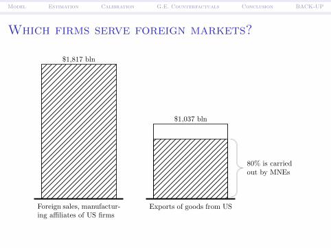
How do firms serve foreign markets?
$1,817 bln
$1,037 bln
Foreign sales, manufactur-ing affiliates of US firms
Exports of goods from US
Model Estimation Calibration G.E. Counterfactuals Conclusion BACK-UP
Which firms serve foreign markets?
80% is carriedout by MNEs
$1,817 bln
$1,037 bln
Foreign sales, manufactur-ing affiliates of US firms
Exports of goods from US

Model Estimation Calibration G.E. Counterfactuals Conclusion BACK-UP
Frameworks for horizontal multinationals
Proximity-concentration trade-off
Firms invest abroad to avoid marginal trade costs (proximitybenefit)Firms export to avoid fixed costs (concentration benefit)
Key references: Helpman, Melitz, and Yeaple (2004), Irrazabal,Moxnes, and Opromolla (2013)
Older work: Markusen (1984), Horstmann and Markusen (1989),Brainard (1997)
Binary choice whether to establish an affiliate in a foreign country
Key assumption: firms cannot use their foreign affiliate to exportto other countries
Model Estimation Calibration G.E. Counterfactuals Conclusion BACK-UP
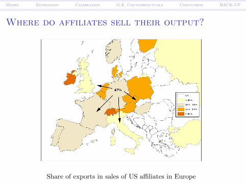
Where do affiliates sell their output?
Share of exports in sales of US affiliates in Europe

Model Estimation Calibration G.E. Counterfactuals Conclusion BACK-UP
Where do affiliates sell their output?
Share of exports in sales of US affiliates in Europe
Model Estimation Calibration G.E. Counterfactuals Conclusion BACK-UP
Tintelnot (2012)
Develops a multi-country general equilibrium framework of tradeand multinational production
Estimates the costs of foreign production with firm-level data onall German multinational firms
Studies the implications of multinational production for classicquestions in international trade:
How do technology shocks in one country affect production andwelfare outcomes in all countries?How do regional trade and investment agreements affectparticipants and non-participants of the agreement?

Model Estimation Calibration G.E. Counterfactuals Conclusion BACK-UP
Tintelnot (2012)
Develops a multi-country general equilibrium framework of tradeand multinational production
Estimates the costs of foreign production with firm-level data onall German multinational firms
Studies the implications of multinational production for classicquestions in international trade:
How do technology shocks in one country affect production andwelfare outcomes in all countries?
How do regional trade and investment agreements affectparticipants and non-participants of the agreement?

Model Estimation Calibration G.E. Counterfactuals Conclusion BACK-UP
Tintelnot (2012)
Develops a multi-country general equilibrium framework of tradeand multinational production
Estimates the costs of foreign production with firm-level data onall German multinational firms
Studies the implications of multinational production for classicquestions in international trade:
How do technology shocks in one country affect production andwelfare outcomes in all countries?How do regional trade and investment agreements affectparticipants and non-participants of the agreement?

Model Estimation Calibration G.E. Counterfactuals Conclusion BACK-UP
Key ingredients of the model
Comparative advantage
Proximity-concentration trade-off
Export platform sales
Firm heterogeneity, monopolistic competition, CES preferences

Model Estimation Calibration G.E. Counterfactuals Conclusion BACK-UP
Key ingredients of the model
Comparative advantage
Proximity-concentration trade-off
Export platform sales
Firm heterogeneity, monopolistic competition, CES preferences

Model Estimation Calibration G.E. Counterfactuals Conclusion BACK-UP
Key ingredients of the model
Comparative advantage
Proximity-concentration trade-off
Export platform sales
Firm heterogeneity, monopolistic competition, CES preferences

Model Estimation Calibration G.E. Counterfactuals Conclusion BACK-UP
Key ingredients of the model
Comparative advantage
Proximity-concentration trade-off
Export platform sales
Firm heterogeneity, monopolistic competition, CES preferences

Model Estimation Calibration G.E. Counterfactuals Conclusion BACK-UP
Fixed costs and export platform sales
Why both?
Model estimated without fixed costs does not generate enoughexport platform sales
Fixed costs explain why most firms concentrate their productionin only a few locations
A model without fixed costs leads to different quantitative answersto welfare and policy questions

Model Estimation Calibration G.E. Counterfactuals Conclusion BACK-UP
Why has this not been done before?
It would be nearly impossible to use e.g. Helpman, Melitz, andYeaple (2004) off the shelf and put export platforms into it.
Hard permutation problem at the firm-level
Key idea for tractability:
Each firm consists of a continuum of productsIn each country in which the firm has a plant, it receivesproduct-location-specific productivity drawsAnalytic solution for the output at the plant-level (underconvenient distributional assumption)Smooth substitutibility between the firm’s plants

Model Estimation Calibration G.E. Counterfactuals Conclusion BACK-UP
Why has this not been done before?
It would be nearly impossible to use e.g. Helpman, Melitz, andYeaple (2004) off the shelf and put export platforms into it.
Hard permutation problem at the firm-level
Key idea for tractability:
Each firm consists of a continuum of products
In each country in which the firm has a plant, it receivesproduct-location-specific productivity drawsAnalytic solution for the output at the plant-level (underconvenient distributional assumption)Smooth substitutibility between the firm’s plants

Model Estimation Calibration G.E. Counterfactuals Conclusion BACK-UP
Why has this not been done before?
It would be nearly impossible to use e.g. Helpman, Melitz, andYeaple (2004) off the shelf and put export platforms into it.
Hard permutation problem at the firm-level
Key idea for tractability:
Each firm consists of a continuum of productsIn each country in which the firm has a plant, it receivesproduct-location-specific productivity draws
Analytic solution for the output at the plant-level (underconvenient distributional assumption)Smooth substitutibility between the firm’s plants

Model Estimation Calibration G.E. Counterfactuals Conclusion BACK-UP
Why has this not been done before?
It would be nearly impossible to use e.g. Helpman, Melitz, andYeaple (2004) off the shelf and put export platforms into it.
Hard permutation problem at the firm-level
Key idea for tractability:
Each firm consists of a continuum of productsIn each country in which the firm has a plant, it receivesproduct-location-specific productivity drawsAnalytic solution for the output at the plant-level (underconvenient distributional assumption)
Smooth substitutibility between the firm’s plants

Model Estimation Calibration G.E. Counterfactuals Conclusion BACK-UP
Why has this not been done before?
It would be nearly impossible to use e.g. Helpman, Melitz, andYeaple (2004) off the shelf and put export platforms into it.
Hard permutation problem at the firm-level
Key idea for tractability:
Each firm consists of a continuum of productsIn each country in which the firm has a plant, it receivesproduct-location-specific productivity drawsAnalytic solution for the output at the plant-level (underconvenient distributional assumption)Smooth substitutibility between the firm’s plants

Model Estimation Calibration G.E. Counterfactuals Conclusion BACK-UP
Preview of main quantitative results
Fixed costs of foreign production are quantitatively important:
Without fixed costs multinationals would produce more than twiceas much abroad.Estimated model with fixed costs can match the export platformsales of US MNEs
Effects of a foreign technology shock:
Welfare gains abroad from a US technology improvement are anorder of magnitude larger than in a pure trade model
Effects of regional trade and investment agreements:
CETA could divert around seven percent of European MNE’sproduction from US to Canada

Model Estimation Calibration G.E. Counterfactuals Conclusion BACK-UP
Preview of main quantitative results
Fixed costs of foreign production are quantitatively important:
Without fixed costs multinationals would produce more than twiceas much abroad.
Estimated model with fixed costs can match the export platformsales of US MNEs
Effects of a foreign technology shock:
Welfare gains abroad from a US technology improvement are anorder of magnitude larger than in a pure trade model
Effects of regional trade and investment agreements:
CETA could divert around seven percent of European MNE’sproduction from US to Canada

Model Estimation Calibration G.E. Counterfactuals Conclusion BACK-UP
Preview of main quantitative results
Fixed costs of foreign production are quantitatively important:
Without fixed costs multinationals would produce more than twiceas much abroad.Estimated model with fixed costs can match the export platformsales of US MNEs
Effects of a foreign technology shock:
Welfare gains abroad from a US technology improvement are anorder of magnitude larger than in a pure trade model
Effects of regional trade and investment agreements:
CETA could divert around seven percent of European MNE’sproduction from US to Canada

Model Estimation Calibration G.E. Counterfactuals Conclusion BACK-UP
Preview of main quantitative results
Fixed costs of foreign production are quantitatively important:
Without fixed costs multinationals would produce more than twiceas much abroad.Estimated model with fixed costs can match the export platformsales of US MNEs
Effects of a foreign technology shock:
Welfare gains abroad from a US technology improvement are anorder of magnitude larger than in a pure trade model
Effects of regional trade and investment agreements:
CETA could divert around seven percent of European MNE’sproduction from US to Canada

Model Estimation Calibration G.E. Counterfactuals Conclusion BACK-UP
Related literature
Quantitative models of trade
Eaton and Kortum (2002), Anderson and van Wincoop (2003)
Proximity-concentration trade-off
Horstmann and Markusen (1992), Brainard (1997), Helpman,Melitz, and Yeaple (2004), Irarrazabal, Moxnes, and Opromolla(2012)
Quantitative models of trade and multinational production
Ramondo and Rodriguez-Clare (2012),Arkolakis, Ramondo, Rodriguez-Clare, and Yeaple (2012)

Model Estimation Calibration G.E. Counterfactuals Conclusion BACK-UP
Outline
Model
Estimation with firm-level data
Calibration with aggregate data
G.E. Counterfactuals

Model Estimation Calibration G.E. Counterfactuals Conclusion BACK-UP
Model

Model Estimation Calibration G.E. Counterfactuals Conclusion BACK-UP
Environment
N countries
Representative consumer:
Measure of Lj consumers / workersDixit-Stiglitz preferences, elasticity of substitution σ > 1
Firms:
Measure of Mi firmsCountry of origin i, core productivity level φ, fixed cost vector η,and plant productivity shifter ε
Trade costs τlm to serve country m from country l
Efficiency loss γil for firms from country i in country l

Model Estimation Calibration G.E. Counterfactuals Conclusion BACK-UP
Production technology
Each firm has a measure 1 of differentiated products.
Conditional on plant in l: Firm can produce product υ under CRSwith productivity νl(υ) in country l
Product-level productivities in county l ∈ Z are distributedFrechet:
Pr(νl ≤ x) = exp(−(φεl)
θ(γilx)−θ)
Technical restriction: θ > σ − 1

Model Estimation Calibration G.E. Counterfactuals Conclusion BACK-UP
Firm’s problem and timing
The firm initially observes the following characteristics aboutitself:
Country of origin iCore productivity, φFixed cost vector, η
The firm solves the following problem:1 Select a set of countries Z ∈ Zi in which to build a plant and pay
fixed costs:∑k∈Z ηkwk
2 After plants are selected:Observe vector of plant-specific productivity shifters, ε, and receiveproduct-location-specific productivity drawsDecide for each product which market to serve from whereSet prices for each product
i, φ, η ǫ, product-location-specific productivity draws
Z ∈ Zi For each product and market: l ∈ Z, price
Observe:
Select:

Model Estimation Calibration G.E. Counterfactuals Conclusion BACK-UP
Firm’s problem and timing
The firm initially observes the following characteristics aboutitself:
Country of origin iCore productivity, φFixed cost vector, η
The firm solves the following problem:1 Select a set of countries Z ∈ Zi in which to build a plant and pay
fixed costs:∑k∈Z ηkwk
2 After plants are selected:
Observe vector of plant-specific productivity shifters, ε, and receiveproduct-location-specific productivity drawsDecide for each product which market to serve from whereSet prices for each product
i, φ, η ǫ, product-location-specific productivity draws
Z ∈ Zi For each product and market: l ∈ Z, price
Observe:
Select:

Model Estimation Calibration G.E. Counterfactuals Conclusion BACK-UP
Firm’s problem and timing
The firm initially observes the following characteristics aboutitself:
Country of origin iCore productivity, φFixed cost vector, η
The firm solves the following problem:1 Select a set of countries Z ∈ Zi in which to build a plant and pay
fixed costs:∑k∈Z ηkwk
2 After plants are selected:Observe vector of plant-specific productivity shifters, ε, and receiveproduct-location-specific productivity draws
Decide for each product which market to serve from whereSet prices for each product
i, φ, η ǫ, product-location-specific productivity draws
Z ∈ Zi For each product and market: l ∈ Z, price
Observe:
Select:

Model Estimation Calibration G.E. Counterfactuals Conclusion BACK-UP
Firm’s problem and timing
The firm initially observes the following characteristics aboutitself:
Country of origin iCore productivity, φFixed cost vector, η
The firm solves the following problem:1 Select a set of countries Z ∈ Zi in which to build a plant and pay
fixed costs:∑k∈Z ηkwk
2 After plants are selected:Observe vector of plant-specific productivity shifters, ε, and receiveproduct-location-specific productivity drawsDecide for each product which market to serve from where
Set prices for each product
i, φ, η ǫ, product-location-specific productivity draws
Z ∈ Zi For each product and market: l ∈ Z, price
Observe:
Select:

Model Estimation Calibration G.E. Counterfactuals Conclusion BACK-UP
Firm’s problem and timing
The firm initially observes the following characteristics aboutitself:
Country of origin iCore productivity, φFixed cost vector, η
The firm solves the following problem:1 Select a set of countries Z ∈ Zi in which to build a plant and pay
fixed costs:∑k∈Z ηkwk
2 After plants are selected:Observe vector of plant-specific productivity shifters, ε, and receiveproduct-location-specific productivity drawsDecide for each product which market to serve from whereSet prices for each product
i, φ, η ǫ, product-location-specific productivity draws
Z ∈ Zi For each product and market: l ∈ Z, price
Observe:
Select:

Model Estimation Calibration G.E. Counterfactuals Conclusion BACK-UP
Plant-level output
Given a set of countries Z in which the firm built a plant
Firm selects for each product and market the plant with theminimum cost
If l ∈ Z:
rl(i, φ, Z, ε) = κφσ−1θ
∑m
Ym
P 1−σm
(γilwlτlm)−θ εθl(∑k∈Z
(γikwkτkm)−θ εθk
)( θ+1−σθ )

Model Estimation Calibration G.E. Counterfactuals Conclusion BACK-UP
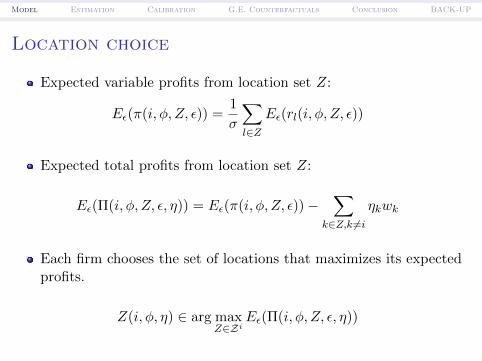
Location choice
Expected variable profits from location set Z:
Eε(π(i, φ, Z, ε)) =1
σ
∑l∈Z
Eε(rl(i, φ, Z, ε))
Expected total profits from location set Z:
Eε(Π(i, φ, Z, ε, η)) = Eε(π(i, φ, Z, ε))−∑
k∈Z,k 6=iηkwk
Each firm chooses the set of locations that maximizes its expectedprofits.
Z(i, φ, η) ∈ arg maxZ∈Zi
Eε(Π(i, φ, Z, ε, η))

Model Estimation Calibration G.E. Counterfactuals Conclusion BACK-UP
Location choice
Expected variable profits from location set Z:
Eε(π(i, φ, Z, ε)) =1
σ
∑l∈Z
Eε(rl(i, φ, Z, ε))
Expected total profits from location set Z:
Eε(Π(i, φ, Z, ε, η)) = Eε(π(i, φ, Z, ε))−∑
k∈Z,k 6=iηkwk
Each firm chooses the set of locations that maximizes its expectedprofits.
Z(i, φ, η) ∈ arg maxZ∈Zi
Eε(Π(i, φ, Z, ε, η))

Model Estimation Calibration G.E. Counterfactuals Conclusion BACK-UP
Motivation to build foreign plants
Proximity to markets
Comparative advantage
Benefits get reduced by efficiency losses of foreign production, γil
Trade-off between these benefits and fixed costs

Model Estimation Calibration G.E. Counterfactuals Conclusion BACK-UP
Aggregation and Equilibrium
Aggregate over the choices of firms (φ, η, ε) from all countries (i).
Profits are distributed to consumers in countries in which thefirms originated
Equilibrium definition is standard (monopolistic competition):
Consumers / Firms optimizeMarkets clearFixed point for price indices and income in every country.

Model Estimation Calibration G.E. Counterfactuals Conclusion BACK-UP
Equilibrium computation
Consumers and firms need to know Al = YlP 1−σl
and wl, l = 1, .., N
in order to make their decisions.
Given parameter vector β, the equilibrium can be computed as asolution for A and w of:
Al(β,w,A) = Al ∀l = 1, .., N
Ldl (β,w,A) = Ll ∀l = 1, .., N − 1

Model Estimation Calibration G.E. Counterfactuals Conclusion BACK-UP
Remarks
Special case: Anderson and van Wincoop (2003)
Model is suitable to address both firm level and aggregate data
Continuum of products and product-location-specific productivityshocks make it feasible to solve and estimate the model

Model Estimation Calibration G.E. Counterfactuals Conclusion BACK-UP
Estimation

Model Estimation Calibration G.E. Counterfactuals Conclusion BACK-UP
Overview of estimation
Data on all German multinationals in 12 Western European andNorth American countries
Observe for each firm
Set of locationsTotal output of each affiliate and of the parent company
Additional data on aggregate manufacturing expenditures, andproxies for bilateral trade costs and price indices
Estimate distribution of fixed costs, ηt,k ∼ logN (µη, ση), unitinput costs, wk = wkγik, and other distributional parameters viaMaximum Likelihood
Fix σ = 6, θ = 7 Estimation of θ

Model Estimation Calibration G.E. Counterfactuals Conclusion BACK-UP
Intuition for identification
The intensive margin – how much do firms produce in a countryrelative to home – identifies the unit input cost in that country.
The extensive margin – in which sets of countries do the firmsestablish plants – identifies the fixed cost parameters.
The size distribution of firms identifies the core productivity leveldistribution parameters and the noise in the output of the firm thedispersion parameter of the plant-wide productivity shifters.

Model Estimation Calibration G.E. Counterfactuals Conclusion BACK-UP
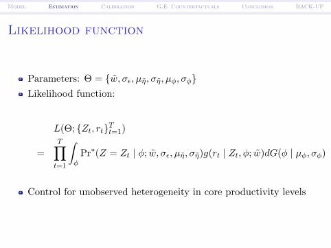
Likelihood function
Parameters: Θ = w, σε, µη, ση, µφ, σφLikelihood function:
L(Θ; Zt, rtTt=1)
=
T∏t=1
∫φ
Pr∗(Z = Zt | φ; w, σε, µη, ση)g(rt | Zt, φ; w)dG(φ | µφ, σφ)
Control for unobserved heterogeneity in core productivity levels
Model Estimation Calibration G.E. Counterfactuals Conclusion BACK-UP
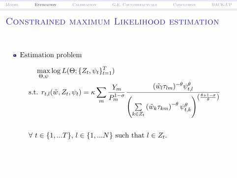
Constrained maximum Likelihood estimation
Estimation problem
maxΘ,ψ
logL(Θ; Zt, ψtTt=1)
s.t. rt,l(w, Zt, ψt) = κ∑m
Ym
P 1−σm
(wlτlm)−θψθt,l( ∑k∈Zt
(wkτkm)−θ ψθt,k
)( θ+1−σθ )
∀ t ∈ 1, ...T, l ∈ 1, ...N such that l ∈ Zt.
Model Estimation Calibration G.E. Counterfactuals Conclusion BACK-UP
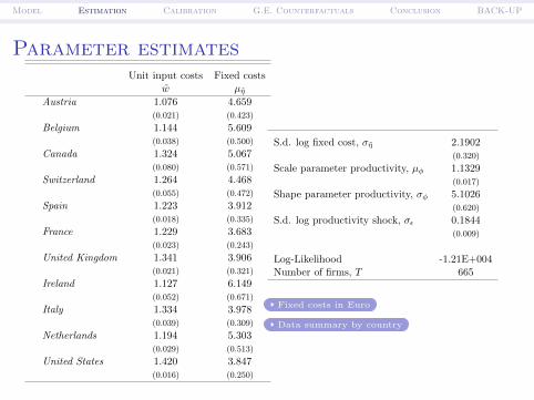
Parameter estimatesUnit input costs Fixed costs
w µηAustria 1.076 4.659
(0.021) (0.423)
Belgium 1.144 5.609(0.038) (0.500)
Canada 1.324 5.067(0.080) (0.571)
Switzerland 1.264 4.468(0.055) (0.472)
Spain 1.223 3.912(0.018) (0.335)
France 1.229 3.683(0.023) (0.243)
United Kingdom 1.341 3.906(0.021) (0.321)
Ireland 1.127 6.149(0.052) (0.671)
Italy 1.334 3.978(0.039) (0.309)
Netherlands 1.194 5.303(0.029) (0.513)
United States 1.420 3.847(0.016) (0.250)
S.d. log fixed cost, ση 2.1902(0.320)
Scale parameter productivity, µφ 1.1329(0.017)
Shape parameter productivity, σφ 5.1026(0.620)
S.d. log productivity shock, σε 0.1844(0.009)
Log-Likelihood -1.21E+004Number of firms, T 665
Fixed costs in Euro
Data summary by country

Model Estimation Calibration G.E. Counterfactuals Conclusion BACK-UP
Decomposing the sources of home bias inproduction
Average share of foreign production in the output of GermanMNEs across counterfactual production costs
Data Model No fixed Same unit No fixedcosts input costs as costs and same
in Germany unit input costsas in Germany
0.288 0.317 0.716 0.676 0.883(0.013) (0.009) (0.021) (0.001)

Model Estimation Calibration G.E. Counterfactuals Conclusion BACK-UP
Calibration

Model Estimation Calibration G.E. Counterfactuals Conclusion BACK-UP
Calibration of the general equilibrium
Data:
Bilateral manufacturing trade flows from OECDBilateral MP from Ramondo, Rodriguez-Clare, and Tintelnot (inprocess)Size of labor force and skill level from Barro and Lee (2010)Gravity variables from CEPIIEstimates of German MNEs’ production costs in variousdestination countries
Model Estimation Calibration G.E. Counterfactuals Conclusion BACK-UP
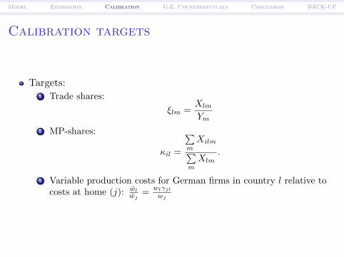
Calibration targets
Targets:1 Trade shares:
ξlm =Xlm
Ym
2 MP-shares:
κil =
∑mXilm∑
mXlm
.
3 Variable production costs for German firms in country l relative tocosts at home (j): wl
wj=
wlγjlwj

Model Estimation Calibration G.E. Counterfactuals Conclusion BACK-UP
Restrictions on parameters
Variable iceberg trade and MP costs
τlm = βτconst(distlm)βτdist(βτcontig)
contiglm(βτlang)languagelm for l 6= m
γil = βγconst(distil)βγdist(βγcontig)
contigil(βγlang)languageil for i 6= l
Fixed MP costs: ηl ∼ logN (ln fil, βfσ)
fil = βfconst(distil)βfdist(βfcontig)
contigil(βflang)languageil for i 6= l
Fixed endowments: Li, Mi
Fixed parameters:
σ = 6, θ = 7σε = 0φ ∼ Pareto with shape parameter 5.5

Model Estimation Calibration G.E. Counterfactuals Conclusion BACK-UP
Calibration procedure
Fit of targets
d(β,w,A) =
ξ(β,w,A)− ξκ(β,w,A)− κw(β,w,A)
wj− w
wj
Calibration problem
minβ,w,A
d(β,w,A)′d(β,w,A)
subject to:
Al(β,w,A) = Al ∀l = 1, .., N
Ldl (β,w,A) = Ll ∀l = 1, .., N − 1

Model Estimation Calibration G.E. Counterfactuals Conclusion BACK-UP
Trade and MP costs estimates
Pure trade Global productionmodel model
Trade costconstant 0.722 0.789distance 0.139 0.121language 0.922 0.929contiguity 0.934 0.925
Variable MP costconstant 1.259distance 0.006language 0.962contiguity 0.963
Fixed MP costconstant 0.089distance 0.073language 1.025contiguity 1.105dispersion 0.299
Norm trade fit 0.258 0.262Norm MP fit 0.158

Model Estimation Calibration G.E. Counterfactuals Conclusion BACK-UP
Share of exports in production of USaffiliates: Data and Model
0 0.1 0.2 0.3 0.4 0.5 0.6 0.7 0.8 0.9 10
0.1
0.2
0.3
0.4
0.5
0.6
0.7
0.8
0.9
1
AUT
BEL
CAN
CHE
DEU
ESPFRA
GBR
IRL
ITA
NLD
model
data
Figure: Export platform shares for US multinationals - data and model

Model Estimation Calibration G.E. Counterfactuals Conclusion BACK-UP
G.E. Counterfactuals

Model Estimation Calibration G.E. Counterfactuals Conclusion BACK-UP
The benefits of foreign technology
How does a technology shock in one country affect production andwelfare outcomes in all countries?
Suppose all US firms improve their productivity by 20 percent.
With and without multinational production, US welfare improvesby around 20 percent.

Model Estimation Calibration G.E. Counterfactuals Conclusion BACK-UP
Benefits from US technology improvement
Pure trade Global productionmodel model
Austria 0.45 14.52Belgium 0.26 9.34Canada 3.53 28.69Switzerland 0.37 9.26Germany 0.15 7.07Spain 0.26 14.11France 0.17 7.76United Kingdom 0.32 13.60Ireland 1.12 20.93Italy 0.18 10.92Netherlands 0.32 13.03United States 100.00 100.00
Results without increasing returns

Model Estimation Calibration G.E. Counterfactuals Conclusion BACK-UP
Effects from CETA
Comprehensive Economic and Trade Agreement (Canada and EU)
What are the effects on signatory countries and the United States?
My model is particularly suitable to address this question:
Trade costs between US and Canada are lowSome European firms want to have only one plant in North AmericaRe-optimization by multinational firms induces a third-countryeffect additional to the terms of trade effect.

Model Estimation Calibration G.E. Counterfactuals Conclusion BACK-UP
Effects from CETA
Comprehensive Economic and Trade Agreement (Canada and EU)
What are the effects on signatory countries and the United States?
My model is particularly suitable to address this question:
Trade costs between US and Canada are low
Some European firms want to have only one plant in North AmericaRe-optimization by multinational firms induces a third-countryeffect additional to the terms of trade effect.

Model Estimation Calibration G.E. Counterfactuals Conclusion BACK-UP
Effects from CETA
Comprehensive Economic and Trade Agreement (Canada and EU)
What are the effects on signatory countries and the United States?
My model is particularly suitable to address this question:
Trade costs between US and Canada are lowSome European firms want to have only one plant in North America
Re-optimization by multinational firms induces a third-countryeffect additional to the terms of trade effect.

Model Estimation Calibration G.E. Counterfactuals Conclusion BACK-UP
Effects from CETA
Comprehensive Economic and Trade Agreement (Canada and EU)
What are the effects on signatory countries and the United States?
My model is particularly suitable to address this question:
Trade costs between US and Canada are lowSome European firms want to have only one plant in North AmericaRe-optimization by multinational firms induces a third-countryeffect additional to the terms of trade effect.
Model Estimation Calibration G.E. Counterfactuals Conclusion BACK-UP
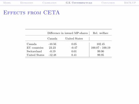
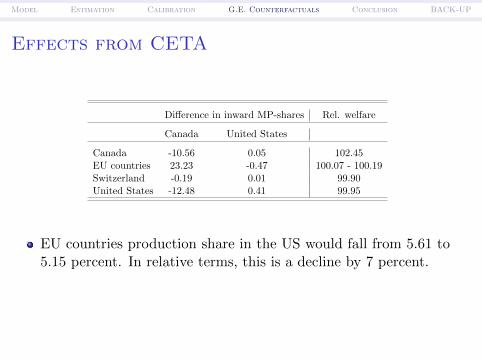
Effects from CETA
Difference in inward MP-shares Rel. welfare
Canada United States
Canada -10.56 0.05 102.45EU countries 23.23 -0.47 100.07 - 100.19Switzerland -0.19 0.01 99.90United States -12.48 0.41 99.95
EU countries production share in the US would fall from 5.61 to5.15 percent. In relative terms, this is a decline by 7 percent.
The overall share of foreign production in the US would fall by 6percent.
Canada would experience the largest welfare gains.
Model Estimation Calibration G.E. Counterfactuals Conclusion BACK-UP
Effects from CETA
Difference in inward MP-shares Rel. welfare
Canada United States
Canada -10.56 0.05 102.45EU countries 23.23 -0.47 100.07 - 100.19Switzerland -0.19 0.01 99.90United States -12.48 0.41 99.95
EU countries production share in the US would fall from 5.61 to5.15 percent. In relative terms, this is a decline by 7 percent.
The overall share of foreign production in the US would fall by 6percent.
Canada would experience the largest welfare gains.

Model Estimation Calibration G.E. Counterfactuals Conclusion BACK-UP
The gains from Trade and MP
The gains from trade:
The real income changes,YP
Y nt
Pnt
, are similar to a pure trade model
Large distributional effects: Profits rise much more than real wages.
The gains from MP:
The real income changes from MP are smaller.Firms real profits fall considerably; change in real wages is similarto disallowing trade.
Remark: Free entry may lead to different welfare outcomes (futurework).

Model Estimation Calibration G.E. Counterfactuals Conclusion BACK-UP
The gains from Trade and MP
The gains from trade:
The real income changes,YP
Y nt
Pnt
, are similar to a pure trade model
Large distributional effects: Profits rise much more than real wages.
The gains from MP:
The real income changes from MP are smaller.
Firms real profits fall considerably; change in real wages is similarto disallowing trade.
Remark: Free entry may lead to different welfare outcomes (futurework).

Model Estimation Calibration G.E. Counterfactuals Conclusion BACK-UP
The gains from Trade and MP
The gains from trade:
The real income changes,YP
Y nt
Pnt
, are similar to a pure trade model
Large distributional effects: Profits rise much more than real wages.
The gains from MP:
The real income changes from MP are smaller.Firms real profits fall considerably; change in real wages is similarto disallowing trade.
Remark: Free entry may lead to different welfare outcomes (futurework).

Model Estimation Calibration G.E. Counterfactuals Conclusion BACK-UP
The gains from Trade and MP
The gains from trade:
The real income changes,YP
Y nt
Pnt
, are similar to a pure trade model
Large distributional effects: Profits rise much more than real wages.
The gains from MP:
The real income changes from MP are smaller.Firms real profits fall considerably; change in real wages is similarto disallowing trade.
Remark: Free entry may lead to different welfare outcomes (futurework).

Model Estimation Calibration G.E. Counterfactuals Conclusion BACK-UP

Model Estimation Calibration G.E. Counterfactuals Conclusion BACK-UP
———————————————————————————————
Conclusion
Main contributions:
A new framework that tractably handles multinational firms thatengage in export platform sales and that face fixed costs of foreigninvestment.
Quantification of the size and importance of fixed costs of foreigninvestment both in partial and general equilibrium
Demonstrated the usefulness of the framework for current policyanalysis
Extensions / future applications:
Competition for multinationals by national governments.

Model Estimation Calibration G.E. Counterfactuals Conclusion BACK-UP
Thank you for your attention!

Model Estimation Calibration G.E. Counterfactuals Conclusion BACK-UP
Back-up

Model Estimation Calibration G.E. Counterfactuals Conclusion BACK-UP
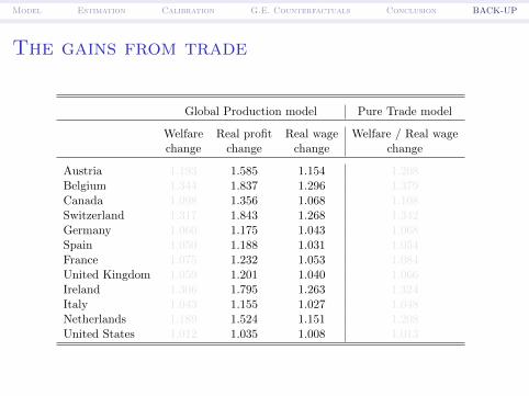
The gains from trade
Global Production model Pure Trade model
Welfare Real profit Real wage Welfare / Real wagechange change change change
Austria 1.193 1.585 1.154 1.208Belgium 1.344 1.837 1.296 1.379Canada 1.098 1.356 1.068 1.108Switzerland 1.317 1.843 1.268 1.342Germany 1.060 1.175 1.043 1.068Spain 1.050 1.188 1.031 1.054France 1.075 1.232 1.053 1.084United Kingdom 1.059 1.201 1.040 1.066Ireland 1.306 1.795 1.263 1.324Italy 1.043 1.155 1.027 1.048Netherlands 1.189 1.524 1.151 1.208United States 1.012 1.035 1.008 1.013
Model Estimation Calibration G.E. Counterfactuals Conclusion BACK-UP
The gains from trade
Global Production model Pure Trade model
Welfare Real profit Real wage Welfare / Real wagechange change change change
Austria 1.193 1.585 1.154 1.208Belgium 1.344 1.837 1.296 1.379Canada 1.098 1.356 1.068 1.108Switzerland 1.317 1.843 1.268 1.342Germany 1.060 1.175 1.043 1.068Spain 1.050 1.188 1.031 1.054France 1.075 1.232 1.053 1.084United Kingdom 1.059 1.201 1.040 1.066Ireland 1.306 1.795 1.263 1.324Italy 1.043 1.155 1.027 1.048Netherlands 1.189 1.524 1.151 1.208United States 1.012 1.035 1.008 1.013

Model Estimation Calibration G.E. Counterfactuals Conclusion BACK-UP
The gains from multinational production
Global Production model
Welfare Real profit Real wagechange change change
Austria 1.017 0.740 1.073Belgium 1.015 0.746 1.069Canada 1.021 0.779 1.069Switzerland 1.018 0.731 1.075Germany 1.006 0.879 1.031Spain 1.011 0.817 1.049France 1.008 0.857 1.038United Kingdom 1.011 0.832 1.047Ireland 1.021 0.684 1.088Italy 1.009 0.844 1.042Netherlands 1.011 0.783 1.056United States 1.002 0.956 1.012

Model Estimation Calibration G.E. Counterfactuals Conclusion BACK-UP
The gains from openness
Global Production model
Welfare Real profit Real wagechange change change
Austria 1.262 0.918 1.331Belgium 1.440 1.058 1.516Canada 1.154 0.880 1.208Switzerland 1.414 1.015 1.494Germany 1.083 0.947 1.110Spain 1.076 0.870 1.117France 1.104 0.939 1.137United Kingdom 1.089 0.896 1.127Ireland 1.400 0.938 1.492Italy 1.065 0.891 1.100Netherlands 1.245 0.965 1.301United States 1.018 0.970 1.027

Model Estimation Calibration G.E. Counterfactuals Conclusion BACK-UP
Benefits from US technology improvementRestricted global production model without fixed cost
Relative to benchmark Relative to US gains
Austria 1.018 8.5042Belgium 1.0106 4.9942Canada 1.0219 10.3312Switzerland 1.0152 7.1452Germany 0.9993 -0.312Spain 1.0033 1.5672France 1.0001 0.0656United Kingdom 1.0009 0.4332Ireland 1.028 13.223Italy 1.0008 0.3998Netherlands 1.0088 4.1482United States 1.2121 100
back

Model Estimation Calibration G.E. Counterfactuals Conclusion BACK-UP
Demand
Utility of representative consumer in country j
U j ≡
∫Ω
1∫0
qj(ω, υ)(σ−1)/σdυdω
σ/(σ−1)
.
Goods are substitutes, σ > 1
The quantity demanded in country j of variety υ supplied by firmω is
qj(ω, υ) = pj(ω, υ)−σYj
P 1−σj
.

Model Estimation Calibration G.E. Counterfactuals Conclusion BACK-UP
Demand
Utility of representative consumer in country j
U j ≡
∫Ω
1∫0
qj(ω, υ)(σ−1)/σdυdω
σ/(σ−1)
.
Goods are substitutes, σ > 1
The quantity demanded in country j of variety υ supplied by firmω is
qj(ω, υ) = pj(ω, υ)−σYj
P 1−σj
.

Model Estimation Calibration G.E. Counterfactuals Conclusion BACK-UP
Demand
Expenditure on goods of firm ω
sj(ω) = pj(ω)1−σ Yj
P 1−σj
.
Firm level price index
pj(ω) ≡
1∫0
pj(ω, υ)1−σdυ
1/(1−σ)
Aggregate price index in country j
Pj ≡
∫Ωj
pj(ω)(1−σ)dω
1/(1−σ)
.
BACK

Model Estimation Calibration G.E. Counterfactuals Conclusion BACK-UP
Demand
Expenditure on goods of firm ω
sj(ω) = pj(ω)1−σ Yj
P 1−σj
.
Firm level price index
pj(ω) ≡
1∫0
pj(ω, υ)1−σdυ
1/(1−σ)
Aggregate price index in country j
Pj ≡
∫Ωj
pj(ω)(1−σ)dω
1/(1−σ)
.
BACK

Model Estimation Calibration G.E. Counterfactuals Conclusion BACK-UP
Demand
Expenditure on goods of firm ω
sj(ω) = pj(ω)1−σ Yj
P 1−σj
.
Firm level price index
pj(ω) ≡
1∫0
pj(ω, υ)1−σdυ
1/(1−σ)
Aggregate price index in country j
Pj ≡
∫Ωj
pj(ω)(1−σ)dω
1/(1−σ)
.
BACK
Model Estimation Calibration G.E. Counterfactuals Conclusion BACK-UP
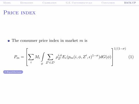
Price index
The consumer price index in market m is
Pm =
∑i
Mi
∫φ
∑Z′∈Zi
ρi,φZ′Eε(pm(i, φ, Z ′, ε)1−σ)dG(φ)
1/(1−σ)
(1)
Equilibrium

Model Estimation Calibration G.E. Counterfactuals Conclusion BACK-UP
Labor market clearing
Labor market clearing condition
wkLk =σ − 1
σ
∑m
Xkm
+∑i 6=k
Mi
∫φ
∫η
∑Z∈∆i
k
1 [Z = Z(i, φ, η)] fikηkwkdF (η)dG(φ)
(2)
Set of location vectors that includes a location in country k:∆ik = Z ∈ Zi | Zk = 1
Equilibrium
Equilibrium computation

Model Estimation Calibration G.E. Counterfactuals Conclusion BACK-UP
Income and Current account balance
Income in country m
Ym = wmLm
+Mm
∫φ
∫η
∑Z∈Zm
1 [Z = Z(i, φ, η)]Eε(Π|i, φ, Z, ε, η)
dF (η)dG(φ)
(3)
Current account balance implies that∑l
Xlm = Ym
Equilibrium

Model Estimation Calibration G.E. Counterfactuals Conclusion BACK-UP
Income and Current account balance
Income in country m
Ym = wmLm
+Mm
∫φ
∫η
∑Z∈Zm
1 [Z = Z(i, φ, η)]Eε(Π|i, φ, Z, ε, η)
dF (η)dG(φ)
(3)
Current account balance implies that∑l
Xlm = Ym
Equilibrium

Model Estimation Calibration G.E. Counterfactuals Conclusion BACK-UP
Equilibrium definition
Given τij , γij ,Mi, F (η), G(φ), H(ε),Z i,∀i, j = 1, ..., N , a globalproduction equilibrium is a set of wages, wi, price indices, Pi, income,Yi, allocations for the representative consumer, q(ω, υ), prices,pm(i, φ, Z, ε) , and location choices, Z(i, φ, η), for the firm, such that
(i) q(ω, υ) is the solution of the consumer’s optimization problem.
(ii) pm(i, φ, Z, ε) and Z(i, φ, η) solve the firm profit maximizationproblem.
(iii) Pi satisfies equation (1).
(iv) The labor market clearing condition, (2), holds.
(v) Ym satisfies equation (3).
Equilibrium overview

Model Estimation Calibration G.E. Counterfactuals Conclusion BACK-UP
Estimation of dispersion parameter ofproduct-level productivity distribution
Product-level sales to market m are distributed Frechet withdispersion parameter θ
σ−1 .
Ideally I would estimate θσ−1 from firm-product bilateral export
data or sales data in particular country.
Data for entire manufacturing sector would be most appropriate.
When using car model sales data in five European countriesavailable from Goldberg and Verboven (2001) I find an estimate ofθ
σ−1 = 1.02.
BACK

Model Estimation Calibration G.E. Counterfactuals Conclusion BACK-UP
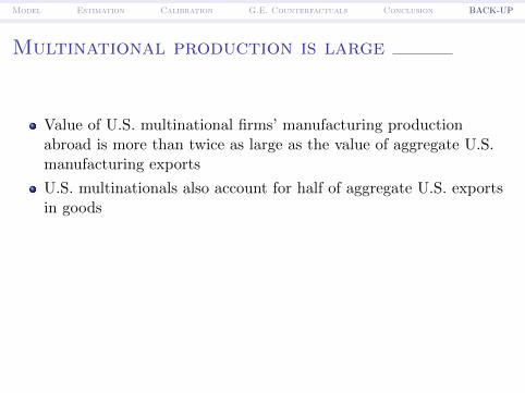
Multinational production is large
Value of U.S. multinational firms’ manufacturing productionabroad is more than twice as large as the value of aggregate U.S.manufacturing exports
U.S. multinationals also account for half of aggregate U.S. exportsin goods
In North America and Western Europe, between 47 percent(Belgium) and 14 percent (U.S.) of output is produced by affiliatesof foreign multinationals.
Foreign output of U.S. multinationals have been growing fasterthan U.S. trade over the last decade.
Model Estimation Calibration G.E. Counterfactuals Conclusion BACK-UP
Multinational production is large
Value of U.S. multinational firms’ manufacturing productionabroad is more than twice as large as the value of aggregate U.S.manufacturing exports
U.S. multinationals also account for half of aggregate U.S. exportsin goods
In North America and Western Europe, between 47 percent(Belgium) and 14 percent (U.S.) of output is produced by affiliatesof foreign multinationals.
Foreign output of U.S. multinationals have been growing fasterthan U.S. trade over the last decade.
Model Estimation Calibration G.E. Counterfactuals Conclusion BACK-UP
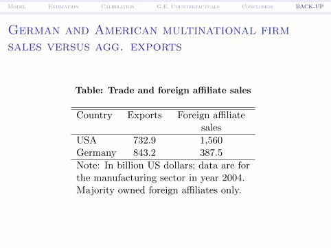
German and American multinational firmsales versus agg. exports
Table: Trade and foreign affiliate sales
Country Exports Foreign affiliatesales
USA 732.9 1,560Germany 843.2 387.5
Note: In billion US dollars; data are forthe manufacturing sector in year 2004.Majority owned foreign affiliates only.

Model Estimation Calibration G.E. Counterfactuals Conclusion BACK-UP
Rewriting the conditional density ofrevenues
g(rt | Zt, φ; w) = |Jt(φ; w)|∏l∈Zt
h
(ψt,l(w)
φ| σε)
BACK

Model Estimation Calibration G.E. Counterfactuals Conclusion BACK-UP
Probability of location choice
Probability that firm with core productivity φ selects vector Zt:
Pr(Z = Zt | φt; w, σε, µη, ση)
=
∫η
Eε(Π(φt, Z, ε, η;σε, w)) ≥ Eε(Π(φt, Z′, ε, η;σε, w)) ∀Z ′ ∈ Zi
dF (η;µη, ση)
Taking into account selection of the data:
Pr∗(Z = Zt | φt; w, σε, µη, ση) =Pr(Z = Zt | φ; w, σε, µη, ση)
1− Pr(Z = Zdomestic | φ; w, σε, µη, ση).
BACK

Model Estimation Calibration G.E. Counterfactuals Conclusion BACK-UP
Preliminary evidence for barriers tomultinational production
Table: Foreign production shares
Cardinality Number Mean share Mean shareproduction of firms of foreign of foreignlocations firm production gross production
2 474 0.26 0.373 102 0.32 0.544 40 0.35 0.655 23 0.39 0.716 14 0.46 0.75≥ 7 12 0.48 0.80
all 665 0.29 0.44
Note: Statistics for German MNE activities in 12 Western Europeanand North American countries.

Model Estimation Calibration G.E. Counterfactuals Conclusion BACK-UP
German multinationals’ activities by country
Country Number Mean Medianoutput output
Austria 91 76.3 34Belgium 45 235.3 37Canada 36 536.0 28.5Switzerland 70 58.3 17Germany 665 625.8 98Spain 117 191.9 32France 191 107.7 30United Kingdom 121 119.4 23Ireland 18 36.3 19.5Italy 100 65.0 27.5Netherlands 46 83.1 25United States 211 569.0 26
Notes: Output in million Euro. Source: MiDi database.
Parameter Estimates

Model Estimation Calibration G.E. Counterfactuals Conclusion BACK-UP
Fixed costs in Euro
Country Mean fixed cost of firms who set up a plantin the respective country in million Euro
Austria 7.107(1.338)
Belgium 18.063(7.515)
Canada 11.718(6.497)
Switzerland 5.814(2.715)
Spain 7.370(2.474)
France 7.037(1.423)
United Kingdom 6.653(1.966)
Ireland 6.069(1.665)
Italy 6.103(1.041)
Netherlands 7.499(2.332)
United States 6.799(1.257)
BACK
Model Estimation Calibration G.E. Counterfactuals Conclusion BACK-UP
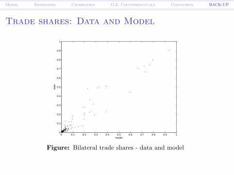
Trade shares: Data and Model
0 0.1 0.2 0.3 0.4 0.5 0.6 0.7 0.8 0.9 10
0.1
0.2
0.3
0.4
0.5
0.6
0.7
0.8
0.9
1
model
data
Figure: Bilateral trade shares - data and model

Model Estimation Calibration G.E. Counterfactuals Conclusion BACK-UP
International production shares: Data andModel
0 0.1 0.2 0.3 0.4 0.5 0.6 0.7 0.8 0.9 10
0.1
0.2
0.3
0.4
0.5
0.6
0.7
0.8
0.9
1
model
data
Figure: Bilateral international production shares - data and model

Model Estimation Calibration G.E. Counterfactuals Conclusion BACK-UP
Variable production costs: Data and Model
1 1.05 1.1 1.15 1.2 1.25 1.3 1.35 1.4 1.451
1.05
1.1
1.15
1.2
1.25
1.3
1.35
1.4
1.45
Calibrated in model
Est
imat
es fr
om m
icro
dat
a
Figure: Variable production costs for German firmsl
BACK