global plate motion frames: toward a unified modelmjelline/453website/eosc... · global plate...
TRANSCRIPT

GLOBAL PLATE MOTION FRAMES:
TOWARD A UNIFIED MODEL
Trond H. Torsvik,1,2,3 R. Dietmar Muller,4 Rob Van der Voo,5 Bernhard Steinberger,1
and Carmen Gaina1
Received 7 May 2007; revised 23 November 2007; accepted 12 February 2008; published 12 August 2008.
[1] Plate tectonics constitutes our primary framework forunderstanding how the Earth works over geologicaltimescales. High-resolution mapping of relative platemotions based on marine geophysical data has followedthe discovery of geomagnetic reversals, mid-ocean ridges,transform faults, and seafloor spreading, cementing the platetectonic paradigm. However, so-called ‘‘absolute platemotions,’’ describing how the fragments of the outer shellof the Earth have moved relative to a reference system suchas the Earth’s mantle, are still poorly understood. Accurateabsolute plate motion models are essential surface boundaryconditions for mantle convection models as well as forunderstanding past ocean circulation and climate ascontinent-ocean distributions change with time. Afundamental problem with deciphering absolute platemotions is that the Earth’s rotation axis and the averagedmagnetic dipole axis are not necessarily fixed to the mantlereference system. Absolute plate motion models based onvolcanic hot spot tracks are largely confined to the last130 Ma and ideally would require knowledge about the
motions within the convecting mantle. In contrast, modelsbased on paleomagnetic data reflect plate motion relative tothe magnetic dipole axis for most of Earth’s history butcannot provide paleolongitudes because of the axialsymmetry of the Earth’s magnetic dipole field. Weanalyze four different reference frames (paleomagnetic,African fixed hot spot, African moving hot spot, and globalmoving hot spot), discuss their uncertainties, and develop aunifying approach for connecting a hot spot track systemand a paleomagnetic absolute plate reference system into a‘‘hybrid’’ model for the time period from the assembly ofPangea (!320 Ma) to the present. For the last 100 Ma weuse a moving hot spot reference frame that takes mantleconvection into account, and we connect this to a pre–100 Ma global paleomagnetic frame adjusted 5! in longitudeto smooth the reference frame transition. Using plate drivingforce arguments and the mapping of reconstructed largeigneous provinces to core–mantle boundary topography, weargue that continental paleolongitudes can be constrainedwithreasonable confidence.
Citation: Torsvik, T. H., R. D. Muller, R. Van der Voo, B. Steinberger, and C. Gaina (2008), Global plate motion frames: Toward aunified model, Rev. Geophys., 46, RG3004, doi:10.1029/2007RG000227.
1. INTRODUCTION
[2] Plates form the outer shell of the Earth, and their pastmovements may be traced using geological data. Platetectonics is a paradigm that attempts to describe the com-plex dynamic evolution of the Earth in terms of rigidlithospheric plates. A simplified form of the theory invokesthe Earth’s heat engine to drive plate motions: mantlematerial heated by isotopic decay rises at spreading ridgeswhere plates diverge and cool during seafloor spreading.
The mantle is cooled by subduction of old, cold lithosphereand is then isotopically heated to rise once again adinfinitum. The theory of plate tectonics has proved success-ful both theoretically and practically, providing a scientificframework for diverse geological disciplines. It is now animportant challenge to integrate plate tectonics into mantledynamics in order to allow a full dynamic treatment of Earthmotion and deformation on all scales. Much progress hasbeen made in understanding the dynamics of mantle con-vection, plate tectonics, and plumes, but a fully integratedmodel incorporating both plate motions and mantle dynam-ics has yet to be realized. Even though links between mantleactivity and plate tectonics are becoming more evident,notably through subsurface tomographic images andadvancements in mineral physics, there is still no generallyaccepted mechanism that consistently explains plate tecton-ics in the framework of mantle convection.
ClickHere
for
FullArticle
1Center for Geodynamics, NGU, Trondheim, Norway.2Also at Physics of Geological Processes, University of Oslo, Oslo, Norway.3Also at School of Geosciences, University of the Witwatersrand,
Johannesburg, South Africa.4School of Geosciences, University of Sydney, Sydney, New South
Wales, Australia.5Department of Geological Sciences, University of Michigan, Ann
Arbor, Michigan, USA.
Copyright 2008 by the American Geophysical Union.
8755-1209/08/2007RG000227$15.00
Reviews of Geophysics, 46, RG3004 / 2008
1 of 44
Paper number 2007RG000227
RG3004

[3] The development of a unifying geodynamic modelrequires the establishment of a global plate motion model.However, the relative motion between tectonic plates mustfirst be determined from fracture zones and ocean floormagnetic anomalies, the oldest of which are only Jurassic inage (!175 Ma) (section 2). Only then can plates be restoredto their paleopositions on the globe using paleomagneticdata (section 3), ‘‘absolute’’ plate rotations from hot spottracks (if one considers hot spots fixed), or, alternatively,using tracks of hot spots that move because of plumeadvection in the mantle (sections 4 and 5). (Italicized termsare defined in the glossary, after the main text.) However,the hot spot track method cannot be used prior to !130 Ma,which is the age at the end of the oldest known track in theSouth Atlantic. That leaves paleomagnetism, with its knownlimitation that it cannot determine motions in longitude, asthe only quantitative way of positioning objects on theglobe during older times.[4] Multiple paleomagnetic and hot spot–mantle refer-
ence frames have been published and compared over thepast decades, but many were constructed without appropri-ate consideration of results based on different data sets andmethods. In this paper we combine interdisciplinary know-how in developing paleomagnetic and hot spot referenceframes, and most importantly, we compare reference frames(section 6) that are generated with the same timescales andplate circuit closure. Ultimately, we combine hot spot andpaleomagnetic frames in order to develop a hybrid globalreference frame for plate motions back to the time whenPangea assembled (section 7). We illustrate how this hybridframe can be used to explore links between surface phe-nomena and deep mantle heterogeneities and briefly discussthe possible causes of kinks, cusps, and longer-durationsmall circle segments in the global apparent polar wander(APW) path for the Pangea supercontinent (section 8).
2. RELATIVE PLATE MOTIONS AND PLATEMOTION CHAINS
[5] The relative motions between tectonic plates can bedetermined from marine geophysical data by the matchingof fracture zones and magnetic anomalies of the same age,corresponding to patterns of paleoridge and paleotransformsegments at a given reconstruction time. Usually, thegeophysical data quality varies substantially, and identifica-tion errors can occur; therefore, the quality of the computedrotations needs to be assessed against the quality of inputdata. Since Bullard et al. [1965] published the first set ofcomputer-generated reconstructions and defined the uncer-tainties attached to the inferred rotations, several othermethods have been proposed to account for uncertaintiesin plate rotations [Hellinger, 1981; Stock and Molnar,1983]. Many of the rotations included in our study werecalculated using Hellinger’s [1981] criteria for goodness offit, associated with uncertainties based on the statisticalapproach developed by Chang [1988] (see Table 1 forreferences to quantitative reconstructions). This methodrequires that isochrons (i.e., magnetic and fracture zone
data of the same age) are divided into great circle segments(Figure 1a). Even though fracture zones are expected tofollow small circles in plate tectonic theory, Hellinger[1981] chose to fit both paleo-mid-ocean ridge and fracturezone segments to great circles because this greatly simpli-fies the least squares fitting routine. The length of fracturesegments used in this approach is so short that the differencebetween a small circle versus a great circle segment isnegligible in this context. The sum of squares of theweighted distances of fixed data points (from one plate)and rotated data points (from the other plate) to the greatcircle segments is minimized in order to derive the rotationparameters and their uncertainties [Hellinger, 1981]. Theuncertainty in a rotation is described by a covariance matrix,which depends on plate boundary geometry, the number ofdata points, and data uncertainties [Chang et al., 1992]. Thismethod allows one to combine independently calculatedrotations and their uncertainties and to compute the result-ing rotation with an uncertainty region that reflects theerrors in the input rotations.[6] The Hellinger [1981] criteria for goodness of fit have
been used mainly for deriving best fit rotations fromconjugate magnetic anomalies and fracture zone data. Formatching boundary between continental and oceanic crustsegments a visual fit is usually preferred because thegeometry of a continent-ocean boundary (COB) can bevery sinuous and difficult to break into great circle seg-ments, as required by Hellinger’s [1981] methodology.Therefore, predrift rotations mostly do not have uncertain-ties attached to them. However, plate circuits can be used toderive the amount of prebreakup displacement (and uncer-tainties). As an example we used the rotations betweenNorth America and Greenland and between North Americaand Eurasia to determine the relative motion and its uncer-tainties between Greenland and Eurasia before breakup(Figure 1b). According to our kinematic model the positionof the COBs should be found within an area that is 45 to77 km wide (from south to north); the uncertainty ofreconstructed points is given by the stage pole uncertaintyellipse calculated for stage pole 31 to 25 (67 to 55 Ma). Arotated Eurasian COB at 55 and 57 Ma (white lines inFigure 1b) fits the end limits of the oldest uncertaintyellipse. Because the ellipse shows the uncertainty of thelocation of the Eurasian COB at 55.9 Ma, this mightindicate that the time of breakup occurred between 55 and57 Ma.[7] Most Euler rotations include insignificant predrift
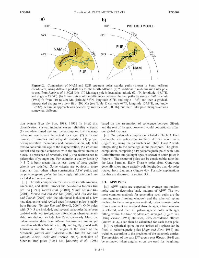
extension prior to initiation of seafloor spreading; as a resultthe majority of Pangea reconstructions essentially useJurassic Euler rotations with minor post-Permian intraplatedeformation. The paleomagnetic coverage from two adja-cent plates is usually not precise enough to determine thisdeformation, but in a few rare cases it has been possible toconstruct predrift relative motion models by fitting portionsof APW paths (Figure 2). In this example, late PaleozoicAPW segments from North America and Europe matcheach other well in the Bullard et al. [1965] reconstruction
RG3004 Torsvik et al.: PLATE MOTION FRAMES
2 of 44
RG3004

TABLE 1. Euler Plate Rotations Used in This Paper
Age(Ma) Latitude Longitude
Angle(deg) Referencea
Europe Versus North America0 0 0 010.95 66.44 132.98 "2.57 1 (Q)20.13 68.91 132.51 "5.09 1 (Q)33.058 68.22 131.53 "7.65 1 (Q)47.906 65.38 138.44 "10.96 1 (Q)53.347 63.07 144.26 "12.82 1 (Q)55.904 56.17 145.06 "13.24 1 (Q)68.737 54.45 147.06 "15.86 1 (Q)79.075 63.4 147.75 "18.48 1 (Q)83.5 66.54 148.91 "19.7 292 66.67 150.26 "20.37 2105 66.85 152.34 "21.49 2118 68.99 154.75 "23.05 2145 68.99 154.75 "23.05 2200 68.99 154.75 "23.64 3 (Q)240 88 27 "38 4 (Q)425 88 27 "38 4 (Q)
Greenland Versus North America0 0 0 033.058 0 0 0 5 (Q)47.906 62.8 260.9 "2.8 5 (Q)53.347 40.64 243.07 "3.615 5 (Q)55.904 20.3 221.8 "3 5 (Q)68.737 52.86 223.6 "6.28 5 (Q)83.5 65.3 "122.45 "11 692 66.6 "119.48 "12.2 6105 67.08 "118.96 "12.99 6118 67.5 "118.48 "13.78 6245 67.5 "118.48 "13.78 6
North America Versus Northwest Africa0 0 0 09.7 80.89 22.82 2.478 8 (Q)19 80.89 23.28 5.244 8 (Q)25.8 79.34 28.56 7.042 8 (Q)33.1 75.99 5.98 9.767 8 (Q)38.4 74.54 0.19 11.918 8 (Q)42.5 74.38 "2.8 13.56 946.3 74.23 "5.01 15.106 8 (Q)49 75.29 "4.26 15.95 952.4 77.34 "1.61 16.963 8 (Q)55.9 80.64 6.57 17.895 8 (Q)65.6 82.74 2.93 20.84 8 (Q)71.1 81.35 "8.32 22.753 8 (Q)73.6 81.11 "10.64 23.74 979.1 78.64 "18.16 26.99 983.5 76.81 "20.59 29.51 989.9 74.33 "22.65 33.86 1094.1 72 "24.39 36.49 10100 69.42 "23.52 40.46 10106.9 68.08 "22.66 45.36 10118.1 66.21 "21 53.19 10119.7 66.09 "20.17 54.45 11125.8 65.97 "19.43 56.63 11133.1 66.14 "18.72 58.03 11139.2 66.24 "18.33 59.71 11148.5 66.24 "18.33 62.14 11154.2 66.7 "15.85 64.9 11170 67.02 "13.17 72.1 12175 66.95 "12.02 75.55 12215 67 348 79 13320 67 348 79 13
Northwest Africa Versus South Africa0 0 0 083.5 0 0 0 14120.4 16.5 6.7 "1.15 14600 16.5 6.7 "1.15 14
TABLE 1. (continued)
Age(Ma) Latitude Longitude
Angle(deg) Referencea
Northeast Africa Versus South Africa0 0 0 083.5 0 0 0 15120.4 40.5 298.6 "0.7 15600 40.4 298.6 "0.7 15
South American Craton (SAC) Versus South Africa0 0 0 02.7 62.2 "39.4 0.83 89.7 62.05 "40.59 3.18 819 58.77 "37.32 7.049 825.8 57.59 "36.27 9.962 833.1 56.17 "33.64 13.41 838.4 57.1 "33 15.912 846.3 56.95 "31.15 19.107 852.4 58.89 "31.18 21.38 855.9 61.35 "32.21 22.273 865.6 63.88 "33.61 24.755 871.6 63.41 "33.38 26.573 879.1 62.92 "34.36 30.992 883.5 61.88 "34.26 33.512 8113 52.4 325 51.3 15120.4 51.6 "35 52.92 14126.7 50.4 "33.5 54.42 14131.7 50 "32.5 55.08 14320 50 "32.5 55.08 14
Parana Versus South Africa (as SAC for #125.7)126.7 50.4 326.5 54.42 15131.7 47.5 326.7 56 15150 47.5 326.7 56.2 15200 47.5 326.7 56.2 15600 47.6 326.7 56.2 14
Colorado Versus South Africa (as SAC for #125.7)126.7 50.4 326.5 54.42 15131.7 47.5 326.7 57 15150 47.5 326.7 57.3 15200 47.5 326.7 58.2 15600 47.5 326.7 58.2 15
Madagascar Versus South Africa0 0 0 0120.4 90 0 0124.1 2.57 "63.33 1.5 20126.7 2.57 "63.33 2.43 20128.2 2.57 "63.33 3.17 20130.2 2.57 "63.33 3.94 20132.1 2.57 "63.33 4.68 20145.1 "0.6 "61.8 8.9 20b
160.0 "14.8 "42.5 15.4 20b
600.0 "14.8 "42.5 15.4 20b
India Versus Madagascar0 0 0 09.9 23.8 33.1 "4.6 20b
20.2 29.6 23.9 "7.5 20b
83.5 22.8 19.1 "51.28 2088 19.8 27.2 "59.16 20120.4 24.02 32.04 "53.01 20124 23.14 33.1 "54.51 20132.1 18.45 31 "61.52 20600 18.45 31 "61.52 20
Australia Versus East Antarctica0 0 0 02.6 "11.6 "139.7 1.65 25 (Q)5.9 "11.59 "139.23 3.83 25 (Q)11.1 "11.90 "142.06 6.79 25 (Q)20.1 "13.39 "145.63 12.05 25 (Q)26.0 "13.80 "146.44 15.92 25 (Q)
RG3004 Torsvik et al.: PLATE MOTION FRAMES
3 of 44
RG3004

for the interval from 310 to 240 Ma. However, no single fitaccommodates the early Mesozoic APW segments for NorthAmerica and Europe. The fit for 240–210 Ma in Figure 2bwas obtained with a gradually changing set of reconstruc-tions using interpolated Euler poles (Table 1). Employingpublished Jurassic stage poles [e.g., Royer et al., 1992] forpre-Jurassic times results in APW paths that are markedlydivergent (Figure 2a); this must clearly be in error given thefact that Laurentia had already collided with Baltica-Avalonia in the middle-to-late Silurian [Torsvik et al.,1996] and remained attached to it during Pangea times.[8] On the basis of the data listed in Table 1 we have
calculated Euler rotations relative to a fixed southern Africa;interpolated rotations (5 Ma intervals) are listed in Table 2.As an example we include a reconstruction for 200 Ma thatalso shows our plate motion chains with respect to a fixedsouthern Africa (Figure 3a). We have also calculated rela-tive velocities of a few selected plates in our analyses. Asexamples we show in Figure 3b calculated plate velocitiesbetween North America and NWAfrica (histogram), Europe(squares), and Greenland (circles). Our model (Table 1)includes predrift extension of 1.75 cm/a between Europeand North America during most of the Triassic and theEarly Jurassic. The bulk of predrift extension occurs in theCretaceous (red squares in Figure 3b) followed by anincrease in relative velocities (3.5 cm/a) between 50 and60 Ma, which coincides with the initial opening (rift to drift)of the northeast Atlantic (!55 Ma). Note that North
Age(Ma) Latitude Longitude
Angle(deg) Referencea
28.5 "13.58 "146.02 17.32 25 (Q)31.0 "13.40 "145.62 18.89 25 (Q)33.5 "13.45 "145.62 20.49 25 (Q)37.5 "14.65 "146.52 22.88 25 (Q)53.3 12.65 32.76 "25.24 1765.6 11.79 32.96 "26.05 1773.6 11.27 33.08 "26.59 1783.5 10.67 33.22 "27.22 1796 8.14 33.34 "27.83 17120.4 11.1 "137.17 29.65 3320 11.1 "137.17 29.65 3
East Antarctica Versus South Africa0 0 0 09.9 8.2 "49.4 1.53 16 (Q)20.2 10.7 "47.9 2.78 16 (Q)33.2 12 "48.4 5.46 16 (Q)40.1 13.6 "41.4 7.47 18 (Q)51.7 8.5 "40.8 10.01 18 (Q)63.1c 11.3 "49.6 11.1 18 (Q)71.1 "1.2 "42.4 12.38 18 (Q)75.5 "4 "40.9 14.03 18 (Q)76.3 "4.6 "40.6 14.39 18 (Q)83.5 "1.3 "34.7 17.78 18 (Q)96 3.1 "38.5 26.5 18 (Q)99 "2.5 "34.03 26.12 19120.4 10.36 153.67 "41.56 20 (Q)124.7 9.45 152.5 "42.91 20 (Q)126.7 9.3 152 "43.71 20 (Q)132.1 8.9 151.2 "46.29 20 (Q)134 8.72 151.1 "47.27 20 (Q)136.7 8.39 150.64 "48.16 20 (Q)137.9 8.25 150.44 "48.55 20 (Q)140.4 7.96 150.04 "49.38 20 (Q)148.1 6.79 146.8 "51.55 20 (Q)160 10.45 148.76 "58.19 20 (Q)360 10.45 148.76 "58.19 20 (Q)
West Antarctica Versus East Antarctica0 0 0 026.55 "18.15 "17.85 0 2133.55 "18.15 "17.85 0.7 22 (Q)43.8 "18.15 "17.85 1.7 2152.2 18.2 162.1 "1.7 361.1 47.225 146.194 "2.967 3600 47.225 146.194 "2.967 3
Lord Howe Rise Versus Australia0 0 0 052.2 0 0 0 23 (Q)53.3c "14.19 130.41 "0.72 23 (Q)55.8c "15.93 133.47 "2.11 23 (Q)57.9c "16.93 136.23 "3.79 23 (Q)61.2 "4.65 131.51 "4.43 23 (Q)62.5c "4.71 132.68 "5.17 23 (Q)64c "0.19 130.37 "5.46 23 (Q)65.6 "3.99 131.8 "6.73 23 (Q)67.7c "9.04 134.46 "8.83 23 (Q)71.1c "14.72 139.04 "13.08 23 (Q)73.6c "9.53 137.2 "12.94 23 (Q)79 0.37 133.82 "13 23 (Q)83.5 2.70 "43.60 14.60 23 (Q)86 4.06 "42.35 15.51 23 (Q)90 3.27 "42.59 18.34 3600 3.27 "42.59 18.34 3
South Campbell Plateau Versus Lord Howe Rise46.3 "49.8 178.4 "49 2483.5 "49.8 178.4 "49 24
TABLE 1. (continued) TABLE 1. (continued)
Age(Ma) Latitude Longitude
Angle(deg) Referencea
Pacific Versus West Antarctica0 0 0 00.78 64.25 "79.06 0.68 7 (Q)2.58 67.03 "73.72 2.42 7 (Q)5.89 67.91 "77.93 5.42 7 (Q)8.86 69.68 "77.06 7.95 7 (Q)10.9 70.86 "75.96 9.71 7 (Q)12.29 71.75 "73.77 10.92 7 (Q)17.47 73.68 "69.85 15.17 7 (Q)20.1 74.15 "68.7 16.9 7 (Q)24.06 74.72 "67.28 19.55 7 (Q)28.28 74.55 "67.38 22.95 7 (Q)33.54 74.38 "64.74 27.34 7 (Q)42.54 74.9 "51.31 34.54 7 (Q)47.91 74.52 "50.19 37.64 7 (Q)53.35 73.62 "52.5 40.03 7 (Q)61.1 71.38 "55.57 44.9 7 (Q)67.7 68.94 "55.52 49.6 2673.6 66.72 "55.04 53.74 27 (Q)83.5 65.58 "52.38 63.07 27 (Q)
aReferences are 1, Gaina et al. [2002]; 2, Srivastava and Roest [1989]; 3,this study; 4, Bullard et al. [1965]; 5, C. Gaina et al. (manuscript inpreparation, 2008); 6, Roest and Srivastava [1989]; 7, Cande et al. [1995];8,Muller et al. [1997]; 9,Muller et al. [1993]; 10,Muller and Roest [1992];11, Roest et al. [1992]; 12, Klitgord and Schouten [1986]; 13, Torsvik et al.[2002]; 14, Nurnberg and Muller [1991]; 15, Torsvik et al. [2004]; 16,Royer and Chang [1991]; 17, Royer and Rollet [1997]; 18, Bernard et al.[2005]; 19, Marks and Tikku [2001]; 20, R. D. Muller and C. Gaina(manuscript in preparation, 2008); 21, S. C. Cande (personal communica-tion, 2002); 22, Cande et al. [2000]; 23, Gaina et al. [1998]; 24, Sutherland[1995]; 25, Cande and Stock [2004]; 26, J. M. Stock (unpublished data,2002); and 27, Larter et al. [2002]. Q indicates qualitative reconstruction.
bValue is recalculated from other plate rotations and plate circuit closure.cValue is not used in smoothed global moving hot spot frame.
RG3004 Torsvik et al.: PLATE MOTION FRAMES
4 of 44
RG3004

America–NWAfrica predrift extension from 220 to 180 Ma(orange part of the histogram, 0.7 cm/a) was recorded by theformation of complex rift systems (e.g., Newark, Connect-icut, and Fundy basins) and was contemporaneous with theCentral Atlantic Magmatic Province (!200 Ma) that affect-ed vast areas in North America, NW Africa, SW Europe,and South America.
3. GLOBAL PALEOMAGNETIC FRAME
3.1. Plate of Choice Anchoring the Global ReferenceFramework
[9] Paleomagnetic reconstructions derived from paleo-poles or APW path segments constrain the paleolatitude
and the angular orientation of a continent, but its paleo-longitude remains unconstrained. However, this degree offreedom can be minimized by selecting an appropriatereference plate; in other words, if one can determine whichplate (or continent) has moved longitudinally the least sincethe time represented by a reconstruction, then that plateshould be used as the reference plate [Burke and Torsvik,2004]. Africa was surrounded on nearly all sides by mid-ocean ridges after the breakup of Pangea: hence, the ridgepush forces should roughly cancel (see also section 9).
3.2. Paleomagnetic Data Selection
[10] Paleomagnetic data were compiled from originalsources and graded according to Van der Voo’s classifica-
Figure 1. (a) Example of marine magnetic anomaly interpretations (700 data points of chron 6 at20.1 Ma) and resulting Euler pole (EP) (black star) and uncertainty ellipse (red contour around EP) forrelative motion between North America (NAM) and Eurasia (EUR) (note that the ellipse was enlarged3 times in order to be visible on the map). Detailed image shows a subset of the chron 6 interpretation inthe North Atlantic and illustrates Hellinger’s [1981] criterion of fit. Fixed data points are represented byinverted triangles; rotated data points are red triangles. The background shows the vertical gradients offree air gravity that allow identification of fracture zones (FZ) and offsets between spreading segments.Great circles were fitted for data points in each individual spreading segment. For a given rotation themeasure of fit represents the sum of squares of the weighted distances (blue segments perpendicular to thegreat circle segment shown as an example on the NAM isochron). The thick, gray line shows the present-day mid-ocean ridge (MOR); the arrows indicate the direction of spreading on NAM and EUR plates.(b) Magnetic anomaly grid of the NE Atlantic [Verhoef et al., 1996] south of Iceland. Vectors and theiruncertainties show relative motion between Eurasia and Greenland for stage poles 67.7–55.9, 55.9–53.3,53.3–49.7, 49.7–47.9, 47.9–43.7, 43.7–40.1, 40.1–33.1, 33.1–20.1, 20.1–10.9, and 10.9–0.0 Ma. Theprebreakup motion has been calculated by combining North America–Greenland and North America–Eurasia rotations. The thick black lines are continent-ocean boundaries (COBs); the white lines indicatethe reconstructed positions of the Eurasian margin relative to Greenland at 55 and 57 Ma. Note that thesewhite lines outline an area that illustrates the uncertainties in the position of the breakup as suggested bythe 95% confidence errors. Light red transparent areas show the mapped seaward dipping reflectors(SDR): Greenland margin, modified after Hopper et al. [2003], and Eurasian margin from L. Gernigon(personal communication, 2006).
RG3004 Torsvik et al.: PLATE MOTION FRAMES
5 of 44
RG3004
tion system [Van der Voo, 1988, 1993]. In brief, thisclassification system includes seven reliability criteria:(1) well-determined age and the assumption that the mag-netization age equals the actual rock age, (2) sufficientnumber of samples and adequate statistics, (3) properdemagnetization techniques and documentation, (4) fieldtests to constrain the age of the magnetization, (5) structuralcontrol and tectonic coherence with the involved craton orblock, (6) presence of reversals, and (7) no resemblance topaleopoles of younger age. For example, a quality factor Q$ 3 (7 is best) means that at least three of these qualitycriteria are satisfied. Some criteria are obviously moreimportant than others when constructing APW paths, andno paleomagnetic poles that knowingly fail criterion 1 areincluded in our analysis.[11] The data compilation for Laurussia (North America,
Greenland, and stable Europe) and Gondwana follows Vander Voo [1993], Torsvik et al. [2001b], Si and Van der Voo[2001], Torsvik and Van der Voo [2002], and Van der Vooand Torsvik [2004] with the additional inclusion of a fewnew data entries and revised ages for certain poles (notablyfrom Europe [Van der Voo and Torsvik, 2004]). Only poleswith Q $ 3 are included, and several paleopoles have beenupdated with new isotopic age information whenever avail-able. We did not include late Paleozoic–early Mesozoicpaleomagnetic data from Siberia because we are as yetuncertain whether Siberia was fully and tightly joined withLaurussia and the rest of Pangea at the dawn of theMesozoic [Torsvik and Andersen, 2002; Van der Voo andTorsvik, 2004; Cocks and Torsvik, 2007]. Inclusion ofSiberian Trap poles (!251 Ma) [Bowring et al., 1998]
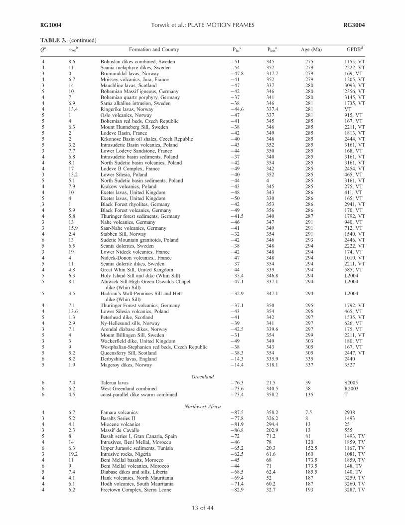
based on the assumption of coherence between Siberiaand the rest of Pangea, however, would not critically affectour global analysis.[12] Our paleopole compilation is listed in Table 3. Each
paleopole was rotated to southern African coordinates(Figure 3a), using the parameters of Tables 1 and 2 whileinterpolating to the same age as the paleopole. The globalcompilation, comprising 419 paleomagnetic poles with LateCarboniferous and younger ages, is shown as south poles inFigure 4. The scatter of poles can be considerable; note thatthe Late Permian–Early Triassic poles from Gondwanagenerally show more easterly pole longitudes than do polesrotated from Laurentia (Figure 4b). Possible explanationsfor this are discussed in section 3.4.
3.3. APW Paths
[13] APW paths are expected to average out randomnoise and to determine basic patterns of APW. The twomost common methods for generating such paths are therunning mean (moving window) and the spherical splinemethod. In the running mean method, paleomagnetic polesfrom a continent are assigned absolute ages, a time windowis selected, and then all paleomagnetic poles with agesfalling within the time window are averaged (Figure 5a).Using Fisher [1953] statistics, 95% confidence ellipses(known as A95) can then be calculated for each mean pole.[14] A spherical spline on the surface of a sphere can be
fitted to paleomagnetic poles [Jupp and Kent, 1987] andweighted according to the precision of the paleopole entries.The precision of the path [Silverman and Waters, 1984] canbe estimated when angular errors are used for weighting.
Figure 2. Comparison of NAM and EUR apparent polar wander paths (shown in South Africancoordinates) using different predrift fits for the North Atlantic. (a) ‘‘Traditional’’ mid-Jurassic Euler poleis used from Royer et al. [1992] (this 170 Ma stage pole is located at latitude 69.1!N, longitude 156.7!E,and angle "23.64!). (b) Minimization of the differences between the two paths by using a Bullard et al.[1965] fit from 310 to 240 Ma (latitude 88!N, longitude 27!E, and angle "38!) and then a gradual,interpolated change to a new fit at 200 Ma (see Table 1) (latitude 69!N, longitude 155.8!E, and angle"23.6!). A similar approach was devised by Torsvik et al. [2001b], but their Euler pole changeover wassomewhat different.
RG3004 Torsvik et al.: PLATE MOTION FRAMES
6 of 44
RG3004
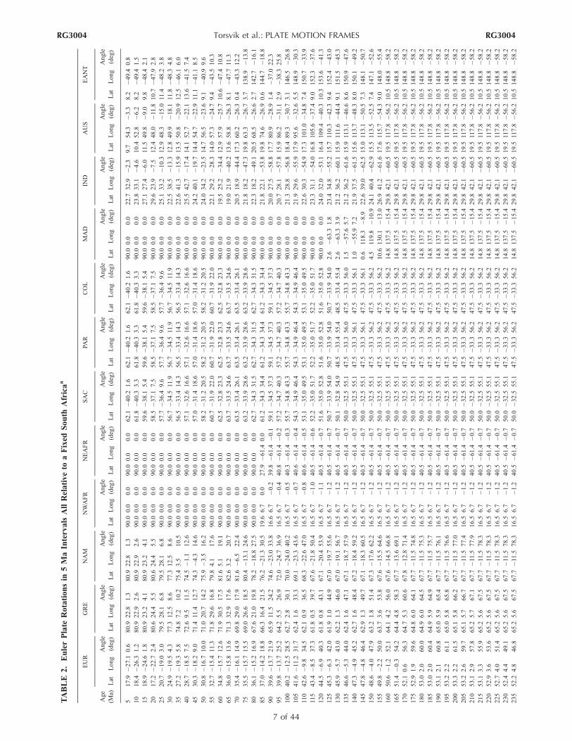
TABLE
2.EulerPlate
Rotationsin
5MaIntervalsAllRelativeto
aFixed
South
Africaa
Age
(Ma)
EUR
GRE
NAM
NWAFR
NEAFR
SAC
PAR
COL
MAD
IND
AUS
EANT
Lat
Long
Angle
(deg)
Lat
Long
Angle
(deg)
Lat
Long
Angle
(deg)
Lat
Long
Angle
(deg)
Lat
Long
Angle
(deg)
Lat
Long
Angle
(deg)
Lat
Long
Angle
(deg)
Lat
Long
Angle
(deg)
Lat
Long
Angle
(deg)
Lat
Long
Angle
(deg)
Lat
Long
Angle
(deg)
Lat
Long
Angle
(deg)
517.9
"27.1
0.6
80.9
22.8
1.3
80.9
22.8
1.3
90.0
0.0
0.0
90.0
0.0
0.0
62.1
"40.2
1.6
62.1
"40.2
1.6
62.1
"40.2
1.6
90.0
0.0
0.0
22.7
32.9
"2.3
9.7
54.3
"3.3
8.2
"49.4
0.8
10
18.4
"26.3
1.2
80.9
22.9
2.6
80.9
22.9
2.6
90.0
0.0
0.0
90.0
0.0
0.0
61.8
"40.3
3.3
61.8
"40.3
3.3
61.8
"40.3
3.3
90.0
0.0
0.0
23.8
33.1
"4.6
10.4
52.8
"6.2
8.2
"49.4
1.5
15
18.9
"24.6
1.8
80.9
23.2
4.1
80.9
23.2
4.1
90.0
0.0
0.0
90.0
0.0
0.0
59.6
"38.1
5.4
59.6
"38.1
5.4
59.6
"38.1
5.4
90.0
0.0
0.0
27.1
27.4
"6.0
11.5
49.8
"9.0
9.8
"48.4
2.1
20
17.2
"22.7
2.4
80.6
24.4
5.5
80.6
24.4
5.5
90.0
0.0
0.0
90.0
0.0
0.0
58.5
"37.1
7.5
58.5
"37.1
7.5
58.5
"37.1
7.5
90.0
0.0
0.0
29.6
23.9
"7.5
12.4
48.0
"11.8
10.7
"47.9
2.8
25
20.7
"19.0
3.0
79.5
28.1
6.8
79.5
28.1
6.8
90.0
0.0
0.0
90.0
0.0
0.0
57.7
"36.4
9.6
57.7
"36.4
9.6
57.7
"36.4
9.6
90.0
0.0
0.0
25.1
33.2
"10.3
12.9
48.3
"15.0
11.4
"48.2
3.8
30
24.9
"19.5
4.3
77.3
12.5
8.6
77.3
12.5
8.6
90.0
0.0
0.0
90.0
0.0
0.0
56.7
"34.5
11.9
56.7
"34.5
11.9
56.7
"34.5
11.9
90.0
0.0
0.0
22.5
38.5
"13.3
12.8
49.9
"18.1
11.8
"48.3
4.8
35
27.2
"19.3
5.8
74.8
7.2
10.2
75.4
3.5
10.5
90.0
0.0
0.0
90.0
0.0
0.0
56.5
"33.4
14.3
56.5
"33.4
14.3
56.5
"33.4
14.3
90.0
0.0
0.0
22.6
41.3
"15.9
13.5
50.8
"20.9
12.5
"46.1
6.0
40
28.7
"18.5
7.5
72.6
9.5
11.5
74.5
"1.1
12.6
90.0
0.0
0.0
90.0
0.0
0.0
57.1
"32.6
16.6
57.1
"32.6
16.6
57.1
"32.6
16.6
90.0
0.0
0.0
25.5
42.7
"17.4
14.1
52.7
"22.1
13.6
"41.5
7.4
45
30.3
"18.2
9.0
71.4
11.4
12.7
74.3
"4.3
14.6
90.0
0.0
0.0
90.0
0.0
0.0
57.0
"31.4
18.6
57.0
"31.4
18.6
57.0
"31.4
18.6
90.0
0.0
0.0
24.2
40.1
"19.7
14.4
54.7
"22.9
11.1
"41.1
8.5
50
30.8
"16.7
10.0
71.0
20.7
14.2
75.9
"3.5
16.2
90.0
0.0
0.0
90.0
0.0
0.0
58.2
"31.2
20.5
58.2
"31.2
20.5
58.2
"31.2
20.5
90.0
0.0
0.0
24.0
34.2
"23.5
14.7
56.5
"23.6
9.1
"40.9
9.6
55
32.7
"15.4
11.3
71.8
29.6
16.8
79.8
4.1
17.6
90.0
0.0
0.0
90.0
0.0
0.0
60.7
"31.9
22.0
60.7
"31.9
22.0
60.7
"31.9
22.0
90.0
0.0
0.0
22.1
29.2
"28.3
14.0
57.3
"24.7
9.4
"43.5
10.3
60
34.8
"15.7
12.6
71.9
30.5
17.5
81.6
5.1
19.1
90.0
0.0
0.0
90.0
0.0
0.0
62.5
"32.8
23.3
62.5
"32.8
23.3
62.5
"32.8
23.3
90.0
0.0
0.0
19.5
25.2
"34.4
12.9
57.9
"25.7
10.6
"47.4
10.8
65
36.0
"15.8
13.6
71.3
32.9
17.6
82.6
3.2
20.7
90.0
0.0
0.0
90.0
0.0
0.0
63.7
"33.5
24.6
63.7
"33.5
24.6
63.7
"33.5
24.6
90.0
0.0
0.0
19.0
21.9
"40.2
13.6
58.8
"26.3
8.1
"47.7
11.3
70
35.4
"16.1
14.9
69.8
29.0
17.9
81.6
"6.5
22.4
90.0
0.0
0.0
90.0
0.0
0.0
63.5
"33.4
26.1
63.5
"33.4
26.1
63.5
"33.4
26.1
90.0
0.0
0.0
20.5
18.9
"44.4
17.3
60.2
"26.3
0.4
"43.3
12.2
75
35.5
"15.7
15.5
69.0
26.6
18.5
80.4
"13.1
24.6
90.0
0.0
0.0
90.0
0.0
0.0
63.2
"33.9
28.6
63.2
"33.9
28.6
63.2
"33.9
28.6
90.0
0.0
0.0
21.8
18.2
"47.3
19.8
63.3
"26.7
3.7
138.9
"13.8
80
36.1
"15.2
16.9
67.6
21.0
19.8
78.2
"18.8
27.5
90.0
0.0
0.0
90.0
0.0
0.0
62.7
"34.3
31.5
62.7
"34.3
31.5
62.7
"34.3
31.5
90.0
0.0
0.0
22.3
18.2
"49.1
20.5
68.5
"26.6
2.7
142.7
"16.1
85
37.0
"14.2
18.8
66.3
16.4
21.5
76.2
"21.3
30.5
19.6
6.7
0.0
27.9
"61.4
0.0
61.2
"34.3
34.4
61.2
"34.3
34.4
61.2
"34.3
34.4
90.0
0.0
0.0
21.8
22.1
"53.8
19.8
74.6
"26.9
0.6
144.7
"18.8
90
39.6
"13.7
21.9
65.9
11.5
24.2
74.6
"23.0
33.8
16.6
6.7
"0.2
39.8
"61.4
"0.1
59.1
"34.5
37.3
59.1
"34.5
37.3
59.1
"34.5
37.3
90.0
0.0
0.0
20.0
27.5
"58.8
17.7
80.9
"28.9
1.4
"37.0
22.3
95
39.8
"13.7
25.2
64.2
5.5
26.9
72.0
"24.7
36.9
16.5
6.7
"0.4
40.8
"61.4
"0.2
57.2
"34.7
40.3
57.2
"34.7
40.3
57.2
"34.7
40.3
90.0
0.0
0.0
20.7
28.1
"57.8
15.9
86.2
"31.1
2.9
"38.3
25.8
100
40.2
"12.5
28.5
62.7
2.8
30.1
70.0
"24.0
40.2
16.5
6.7
"0.5
40.3
"61.4
"0.3
55.7
"34.8
43.3
55.7
"34.8
43.3
55.7
"34.8
43.3
90.0
0.0
0.0
21.3
28.8
"56.8
18.4
89.3
"30.7
3.1
146.5
"26.8
105
41.6
"11.2
31.7
62.4
1.6
33.3
69.1
"23.3
43.6
16.5
6.7
"0.7
40.6
"61.4
"0.4
54.3
"34.9
46.4
54.3
"34.9
46.4
54.3
"34.9
46.4
90.0
0.0
0.0
21.9
29.6
"55.9
17.9
95.6
"32.6
5.5
148.9
"30.3
110
42.6
"9.8
34.5
62.1
0.9
36.5
68.3
"22.6
47.0
16.5
6.7
"0.8
40.6
"61.4
"0.5
53.1
"35.0
49.5
53.1
"35.0
49.5
53.1
"35.0
49.5
90.0
0.0
0.0
22.6
30.3
"54.9
17.3
101.0
"34.8
7.4
150.7
"33.9
115
43.4
"8.5
37.3
61.8
0.5
39.7
67.6
"21.8
50.4
16.5
6.7
"1.0
40.5
"61.4
"0.6
52.2
"35.0
51.7
52.2
"35.0
51.7
52.2
"35.0
51.7
90.0
0.0
0.0
23.3
31.1
"54.0
16.8
105.6
"37.4
9.0
152.3
"37.6
120
44.5
"6.9
40.3
61.8
0.8
43.1
67.1
"20.4
53.9
16.5
6.7
"1.1
40.5
"61.4
"0.7
51.6
"35.0
52.8
51.6
"35.0
52.8
51.6
"35.0
52.8
90.0
0.0
0.0
24.0
32.0
"53.1
16.4
109.4
"40.3
10.3
153.6
"41.3
125
45.3
"6.3
42.0
61.9
1.0
44.9
67.0
"19.7
55.6
16.5
6.7
"1.2
40.5
"61.4
"0.7
50.7
"33.9
54.0
50.7
"33.9
54.0
50.7
"33.9
54.0
2.6
"63.3
1.8
23.4
34.8
"55.2
15.7
110.3
"42.3
9.4
152.4
"43.0
130
45.9
"5.7
43.0
62.2
1.3
46.0
67.0
"19.1
56.7
16.5
6.7
"1.2
40.5
"61.4
"0.7
50.1
"32.8
54.9
48.5
"33.4
55.4
48.5
"33.4
55.4
2.6
"63.3
3.9
21.2
36.2
"60.1
15.9
111.6
"44.4
9.1
151.5
"45.3
135
46.6
"5.3
44.0
62.4
1.6
47.1
67.1
"18.7
57.9
16.5
6.7
"1.2
40.5
"61.4
"0.7
50.0
"32.5
55.1
47.5
"33.3
56.0
47.5
"33.3
56.0
1.5
"57.6
5.7
21.2
36.2
"61.6
15.9
113.1
"46.6
8.6
150.9
"47.6
140
47.3
"4.9
45.2
62.7
1.6
48.4
67.2
"18.4
59.2
16.5
6.7
"1.2
40.5
"61.4
"0.7
50.0
"32.5
55.1
47.5
"33.3
56.1
47.5
"33.3
56.1
1.0
"55.9
7.2
21.9
37.5
"61.5
15.6
113.7
"48.3
8.0
150.1
"49.2
145
47.8
"4.8
46.4
62.9
1.3
49.7
67.1
"18.3
60.5
16.5
6.7
"1.2
40.5
"61.4
"0.7
50.0
"32.5
55.1
47.5
"33.3
56.1
47.5
"33.3
56.1
0.6
118.3
"8.9
22.6
39.0
"62.5
15.0
113.1
"50.5
7.3
148.1
"50.7
150
48.6
"4.0
47.9
63.2
1.8
51.4
67.3
"17.6
62.2
16.5
6.7
"1.2
40.5
"61.4
"0.7
50.0
"32.5
55.1
47.5
"33.3
56.2
47.5
"33.3
56.2
4.5
119.8
"10.9
24.1
40.4
"62.9
15.5
113.5
"52.5
7.4
147.1
"52.6
155
49.8
"2.2
50.0
63.7
3.6
53.8
67.6
"15.5
64.6
16.5
6.7
"1.2
40.5
"61.4
"0.7
50.0
"32.5
55.1
47.5
"33.3
56.2
47.5
"33.3
56.2
10.6
130.1
"13.0
26.9
41.2
"61.6
17.6
115.7
"54.3
9.0
148.0
"55.4
160
50.6
"1.2
52.1
64.1
4.2
56.0
67.6
"14.5
66.8
16.5
6.7
"1.2
40.5
"61.4
"0.7
50.0
"32.5
55.1
47.5
"33.3
56.2
47.5
"33.3
56.2
14.8
137.5
"15.4
29.8
42.1
"60.5
19.5
117.8
"56.2
10.5
148.8
"58.2
165
51.4
"0.3
54.2
64.4
4.8
58.3
67.7
"13.6
69.1
16.5
6.7
"1.2
40.5
"61.4
"0.7
50.0
"32.5
55.1
47.5
"33.3
56.2
47.5
"33.3
56.2
14.8
137.5
"15.4
29.8
42.1
"60.5
19.5
117.8
"56.2
10.5
148.8
"58.2
170
52.1
0.6
56.3
64.7
5.3
60.6
67.8
"12.8
71.4
16.5
6.7
"1.2
40.5
"61.4
"0.7
50.0
"32.5
55.1
47.5
"33.3
56.2
47.5
"33.3
56.2
14.8
137.5
"15.4
29.8
42.1
"60.5
19.5
117.8
"56.2
10.5
148.8
"58.2
175
52.9
1.9
59.6
64.8
6.0
64.1
67.7
"11.5
74.8
16.5
6.7
"1.2
40.5
"61.4
"0.7
50.0
"32.5
55.1
47.5
"33.3
56.2
47.5
"33.3
56.2
14.8
137.5
"15.4
29.8
42.1
"60.5
19.5
117.8
"56.2
10.5
148.8
"58.2
180
53.0
2.0
60.0
64.9
6.0
64.5
67.7
"11.5
75.3
16.5
6.7
"1.2
40.5
"61.4
"0.7
50.0
"32.5
55.1
47.5
"33.3
56.2
47.5
"33.3
56.2
14.8
137.5
"15.4
29.8
42.1
"60.5
19.5
117.8
"56.2
10.5
148.8
"58.2
185
53.0
2.0
60.4
64.9
5.9
64.9
67.7
"11.5
75.7
16.5
6.7
"1.2
40.5
"61.4
"0.7
50.0
"32.5
55.1
47.5
"33.3
56.2
47.5
"33.3
56.2
14.8
137.5
"15.4
29.8
42.1
"60.5
19.5
117.8
"56.2
10.5
148.8
"58.2
190
53.1
2.1
60.8
65.0
5.9
65.4
67.7
"11.5
76.1
16.5
6.7
"1.2
40.5
"61.4
"0.7
50.0
"32.5
55.1
47.5
"33.3
56.2
47.5
"33.3
56.2
14.8
137.5
"15.4
29.8
42.1
"60.5
19.5
117.8
"56.2
10.5
148.8
"58.2
195
53.2
2.2
61.1
65.0
5.8
65.8
67.7
"11.5
76.6
16.5
6.7
"1.2
40.5
"61.4
"0.7
50.0
"32.5
55.1
47.5
"33.3
56.2
47.5
"33.3
56.2
14.8
137.5
"15.4
29.8
42.1
"60.5
19.5
117.8
"56.2
10.5
148.8
"58.2
200
53.3
2.2
61.5
65.1
5.8
66.2
67.7
"11.5
77.0
16.5
6.7
"1.2
40.5
"61.4
"0.7
50.0
"32.5
55.1
47.5
"33.3
56.2
47.5
"33.3
56.2
14.8
137.5
"15.4
29.8
42.1
"60.5
19.5
117.8
"56.2
10.5
148.8
"58.2
205
53.2
2.6
59.7
65.1
5.7
66.7
67.7
"11.5
77.4
16.5
6.7
"1.2
40.5
"61.4
"0.7
50.0
"32.5
55.1
47.5
"33.3
56.2
47.5
"33.3
56.2
14.8
137.5
"15.4
29.8
42.1
"60.5
19.5
117.8
"56.2
10.5
148.8
"58.2
210
53.1
2.9
57.8
65.2
5.7
67.1
67.7
"11.5
77.9
16.5
6.7
"1.2
40.5
"61.4
"0.7
50.0
"32.5
55.1
47.5
"33.3
56.2
47.5
"33.3
56.2
14.8
137.5
"15.4
29.8
42.1
"60.5
19.5
117.8
"56.2
10.5
148.8
"58.2
215
53.1
3.3
55.9
65.2
5.6
67.5
67.7
"11.5
78.3
16.5
6.7
"1.2
40.5
"61.4
"0.7
50.0
"32.5
55.1
47.5
"33.3
56.2
47.5
"33.3
56.2
14.8
137.5
"15.4
29.8
42.1
"60.5
19.5
117.8
"56.2
10.5
148.8
"58.2
220
52.9
3.6
53.6
65.2
5.6
67.5
67.7
"11.5
78.3
16.5
6.7
"1.2
40.5
"61.4
"0.7
50.0
"32.5
55.1
47.5
"33.3
56.2
47.5
"33.3
56.2
14.8
137.5
"15.4
29.8
42.1
"60.5
19.5
117.8
"56.2
10.5
148.8
"58.2
225
52.7
4.0
51.4
65.2
5.6
67.5
67.7
"11.5
78.3
16.5
6.7
"1.2
40.5
"61.4
"0.7
50.0
"32.5
55.1
47.5
"33.3
56.2
47.5
"33.3
56.2
14.8
137.5
"15.4
29.8
42.1
"60.5
19.5
117.8
"56.2
10.5
148.8
"58.2
230
52.4
4.4
49.1
65.2
5.6
67.5
67.7
"11.5
78.3
16.5
6.7
"1.2
40.5
"61.4
"0.7
50.0
"32.5
55.1
47.5
"33.3
56.2
47.5
"33.3
56.2
14.8
137.5
"15.4
29.8
42.1
"60.5
19.5
117.8
"56.2
10.5
148.8
"58.2
235
52.2
4.8
46.8
65.2
5.6
67.5
67.7
"11.5
78.3
16.5
6.7
"1.2
40.5
"61.4
"0.7
50.0
"32.5
55.1
47.5
"33.3
56.2
47.5
"33.3
56.2
14.8
137.5
"15.4
29.8
42.1
"60.5
19.5
117.8
"56.2
10.5
148.8
"58.2
RG3004 Torsvik et al.: PLATE MOTION FRAMES
7 of 44
RG3004

However, the real uncertainty surrounding individualpaleopole positions is a combination of angular errors, ageuncertainties (set at zero for this paper), and uncertaintiessurrounding the geomagnetic field recording of complex-ities such as the averaging of secular variation. Torsvik et al.[1996], for example, developed a routine to give weight tothe data according to their Q factor (section 3.2) so that theAPW path is firmly anchored to the most reliable data.[15] Our global APW path (in southern African coordi-
nates, Figure 5a and Table 4) extends back to 320 Ma whenthe Pangea supercontinent was initially being assembled. Aglobal APW path was first constructed using the runningmean method since this is the simplest method and caneasily be reproduced by others. We used a window length of20 Ma and employed 10 Ma increments, causing onlymoderate smoothing. Increased window length leads to ahigher degree of smoothing.[16] We compare our path of Figure 5a to the APW paths
of Besse and Courtillot [2002] and Schettino and Scotese[2005] and calculate the great circle distance (shortestdistance on a sphere) between mean poles of the sameage (Figure 5b). The mean great circle distance for the entire200 Ma interval is 3.9! ± 3.3! with respect to Besse andCourtillot [2002], with a peak of 11.1! at 200 Ma(Figure 5b). The mean great circle distance is 4.2! ± 3.3!for our comparison with Schettino and Scotese [2005], witha peak of 12.8! at 150 Ma. Most of the differences are likelyto be statistically insignificant, but the open loop between110 and 170 Ma observed in our running mean APW path(Figure 5a) appears as a hairpin with a sharp cusp in theother two paths (Figures 5c and 5d). The reasons for this canbe found in a combination of different data selection, degreeof smoothing, and different Euler rotation parameters.[17] With global data sets that have considerable spread
and ‘‘unclear’’ age progressions, spherical splines (e.g.,weighted purely by angular errors) produce sinuous APWpaths unless they are severely smoothed. Conversely, aspherical spline weighted by the Q factor [Torsvik et al.,1996] will produce APW paths that are anchored to themost reliable data, and this procedure ‘‘reproduces’’ theLate Jurassic–Early Cretaceous loop using moderate-to-high smoothing parameters (red line in Figure 5a). However,a shortcoming of this procedure is that the assignment ofweights to Q factors does not produce output angularuncertainties along the path that have a physical meaning.We therefore opted to first calculate a running mean path(10 Ma window, with increments of 10 Ma, so that there isno window overlap in order to avoid presmoothing) andfound that this leads to a better age progression. Only thenwe applied the spherical spline algorithm to this runningmean path weighted by the mean angular errors (A95). Thisresults in angular output uncertainties that have physicalmeaning. The outcome of this procedure is shown inFigure 5c as the red path with yellow cones of confidenceevery 10 Ma. Using a moderate-to-high smoothing param-eter, we generated a path similar to that of Schettino andScotese [2005]. However, smoothing can lead to removal ofreal, short-duration features in the path. In order to exploreT
ABLE
2.(continued)
Age
(Ma)
EUR
GRE
NAM
NWAFR
NEAFR
SAC
PAR
COL
MAD
IND
AUS
EANT
Lat
Long
Angle
(deg)
Lat
Long
Angle
(deg)
Lat
Long
Angle
(deg)
Lat
Long
Angle
(deg)
Lat
Long
Angle
(deg)
Lat
Long
Angle
(deg)
Lat
Long
Angle
(deg)
Lat
Long
Angle
(deg)
Lat
Long
Angle
(deg)
Lat
Long
Angle
(deg)
Lat
Long
Angle
(deg)
Lat
Long
Angle
(deg)
240
51.9
5.3
44.5
65.2
5.6
67.5
67.7
"11.5
78.3
16.5
6.7
"1.2
40.5
"61.4
"0.7
50.0
"32.5
55.1
47.5
"33.3
56.2
47.5
"33.3
56.2
14.8
137.5
"15.4
29.8
42.1
"60.5
19.5
117.8
"56.2
10.5
148.8
"58.2
245
51.9
5.3
44.5
65.2
5.6
67.5
67.7
"11.5
78.3
16.5
6.7
"1.2
40.4
"61.4
"0.7
50.0
"32.5
55.1
47.5
"33.3
56.2
47.5
"33.3
56.2
14.8
137.5
"15.4
29.8
42.1
"60.5
19.5
117.8
"56.2
10.5
148.8
"58.2
250
51.9
5.3
44.5
65.2
5.6
67.5
67.7
"11.5
78.3
16.5
6.7
"1.2
40.4
"61.4
"0.7
50.0
"32.5
55.1
47.5
"33.3
56.2
47.5
"33.3
56.2
14.8
137.5
"15.4
29.8
42.1
"60.5
19.5
117.8
"56.2
10.5
148.8
"58.2
255
51.9
5.3
44.5
65.2
5.6
67.5
67.7
"11.5
78.3
16.5
6.7
"1.2
40.4
"61.4
"0.7
50.0
"32.5
55.1
47.5
"33.3
56.2
47.5
"33.3
56.2
14.8
137.5
"15.4
29.8
42.1
"60.5
19.5
117.8
"56.2
10.5
148.8
"58.2
260
51.9
5.3
44.5
65.2
5.6
67.5
67.7
"11.5
78.3
16.5
6.7
"1.2
40.4
"61.4
"0.7
50.0
"32.5
55.1
47.5
"33.3
56.2
47.5
"33.3
56.2
14.8
137.5
"15.4
29.8
42.1
"60.5
19.5
117.8
"56.2
10.5
148.8
"58.2
265
51.9
5.3
44.5
65.2
5.6
67.5
67.7
"11.5
78.3
16.5
6.7
"1.2
40.4
"61.4
"0.7
50.0
"32.5
55.1
47.5
"33.3
56.2
47.5
"33.3
56.2
14.8
137.5
"15.4
29.8
42.1
"60.5
19.5
117.8
"56.2
10.5
148.8
"58.2
270
51.9
5.3
44.5
65.2
5.6
67.5
67.7
"11.5
78.3
16.5
6.7
"1.2
40.4
"61.4
"0.7
50.0
"32.5
55.1
47.5
"33.3
56.2
47.5
"33.3
56.2
14.8
137.5
"15.4
29.8
42.1
"60.5
19.5
117.8
"56.2
10.5
148.8
"58.2
275
51.9
5.3
44.5
65.2
5.6
67.5
67.7
"11.5
78.3
16.5
6.7
"1.2
40.4
"61.4
"0.7
50.0
"32.5
55.1
47.5
"33.3
56.2
47.5
"33.3
56.2
14.8
137.5
"15.4
29.8
42.1
"60.5
19.5
117.8
"56.2
10.5
148.8
"58.2
280
51.9
5.3
44.5
65.2
5.6
67.5
67.7
"11.5
78.3
16.5
6.7
"1.2
40.4
"61.4
"0.7
50.0
"32.5
55.1
47.5
"33.3
56.2
47.5
"33.3
56.2
14.8
137.5
"15.4
29.8
42.1
"60.5
19.5
117.8
"56.2
10.4
148.8
"58.2
285
51.9
5.3
44.5
65.2
5.6
67.5
67.7
"11.5
78.3
16.5
6.7
"1.2
40.4
"61.4
"0.7
50.0
"32.5
55.1
47.5
"33.3
56.2
47.5
"33.3
56.2
14.8
137.5
"15.4
29.8
42.1
"60.5
19.5
117.8
"56.2
10.5
148.8
"58.2
290
51.9
5.3
44.5
65.2
5.6
67.5
67.7
"11.5
78.3
16.5
6.7
"1.2
40.4
"61.4
"0.7
50.0
"32.5
55.1
47.5
"33.3
56.2
47.5
"33.3
56.2
14.8
137.5
"15.4
29.8
42.1
"60.5
19.5
117.8
"56.2
10.5
148.8
"58.2
295
51.9
5.3
44.5
65.2
5.6
67.5
67.7
"11.5
78.3
16.5
6.7
"1.2
40.4
"61.4
"0.7
50.0
"32.5
55.1
47.5
"33.3
56.2
47.5
"33.3
56.2
14.8
137.5
"15.4
29.8
42.1
"60.5
19.5
117.8
"56.2
10.5
148.8
"58.2
300
51.9
5.3
44.5
65.2
5.6
67.5
67.7
"11.5
78.3
16.5
6.7
"1.2
40.4
"61.4
"0.7
50.0
"32.5
55.1
47.5
"33.3
56.2
47.5
"33.3
56.2
14.8
137.5
"15.4
29.8
42.1
"60.5
19.5
117.8
"56.2
10.5
148.8
"58.2
305
51.9
5.3
44.5
65.2
5.6
67.5
67.7
"11.5
78.3
16.5
6.7
"1.2
40.4
"61.4
"0.7
50.0
"32.5
55.1
47.5
"33.3
56.2
47.5
"33.3
56.2
14.8
137.5
"15.4
29.8
42.1
"60.5
19.5
117.8
"56.2
10.4
148.8
"58.2
310
51.9
5.3
44.5
65.2
5.6
67.5
67.7
"11.5
78.3
16.5
6.7
"1.2
40.4
"61.4
"0.7
50.0
"32.5
55.1
47.5
"33.3
56.2
47.5
"33.3
56.2
14.8
137.5
"15.4
29.8
42.1
"60.5
19.5
117.8
"56.2
10.5
148.8
"58.2
315
51.9
5.3
44.5
65.2
5.6
67.5
67.7
"11.5
78.3
16.5
6.7
"1.2
40.4
"61.4
"0.7
50.0
"32.5
55.1
47.5
"33.3
56.2
47.5
"33.3
56.2
14.8
137.5
"15.4
29.8
42.1
"60.5
19.5
117.8
"56.2
10.5
148.8
"58.2
320
51.9
5.3
44.5
65.2
5.6
67.5
67.7
"11.5
78.3
16.5
6.7
"1.2
40.4
"61.4
"0.7
50.0
"32.5
55.1
47.5
"33.3
56.2
47.5
"33.3
56.2
14.8
137.5
"15.4
29.8
42.1
"60.5
19.5
117.8
"56.2
10.5
148.8
"58.2
a Only
platesforwhichweuse
paleomagnetic
datato
generatetheglobal
APW
patharelisted.Abbreviationsareas
inFigure
3;Lat,latitude;
Long,longitude.
RG3004 Torsvik et al.: PLATE MOTION FRAMES
8 of 44
RG3004

Figure 3. (a) Preferred relative reconstruction at 200 Ma (with southern Africa held fixed) showing the(continental) plates for which paleomagnetic data have been compiled (Table 3). The determinations ofrelative plate motions (section 2) incorporate a wide variety of data, with the southern African continentalelement serving as the reference continent relative to which the motion of all other plates are determined.In this paper, motion of the African plate is determined in global reference frames using paleomagnetic(section 3), fixed hot spot (section 4), and moving hot spot (section 5) reference frames. Plate chainslinking the Pacific (PAC) and southern Africa (SAFR) follow two different models discussed in the textand illustrated in the inset. Abbreviations are EUR, stable Europe; GRE, Greenland (only Cretaceous-Tertiary poles have been included in the analysis); NAM, North America; NWAFR, northwest Africa;NEAFR, northeast Africa; SAC, main South American craton; PAR_SAL, Parana-Salado subplate; COL,Colorado subplate; IND, India; MAD, Madagascar; EANT, East Antarctica; AUS, Australia; LHR, LordHowe Rise; WANT, West Antarctica; and CAM, southern Campbell Plateau. The intraplate deformationzones in South America and Africa are taken from Torsvik et al. [2004]. (b) Relative plate velocities ofNorth America versus NWAFR (in histogram style), EUR (squares), and GRE (circles). These velocitiesare mean plate velocities calculated for elements in a 10! % 10! grid. The blue histogram and symbols arederived from seafloor spreading models. Black annotated arrows indicate major kinks or cusps in theglobal apparent polar wander path when viewed in North American coordinates (see Figure 8).
RG3004 Torsvik et al.: PLATE MOTION FRAMES
9 of 44
RG3004

TABLE 3. Selected Paleomagnetic Poles
Qa a95b Formation and Country Plat
c Plonc Age (Ma) GPDBd
North America6 4.9 Katherine Creek sediments "78 304 1.5 30606 7 Banks Island deposits "86 120 1.5 32063 9.7 Tschicoma Formation "76 174 5.5 1275, SV3 12.9 Hepburn’s Mesa Formation "81 225 15.5 2288, SV4 6.7 Younger plutons "87 189 22.5 1402, SV3 8.4 Lake City caldera "76 30 23 1300, SV4 5.2 Latir volcanics "81 331 23.5 1299, SV4 6.8 Conejos and Hinsdale Formation "80 343 26 3130, SV4 5.4 Latir extrusives, sediments "80 315 27 1299, SV4 4.4 Mongollon-Datil volcanics "82 323 30 1315, SV3 5 Mongollon-Datil volcanics "83 316 30 2631, SV4 4.3 Mariscal Mountain gabbro "80 5 37 2943, SV3 2.4 Mistastin Lake impact "86 298 40 562, T5 7.7 East Fork Washakia Basin "84 324 44 1632, T4 10.1 Virginia intrusions "86 64 44.5 18655 8 Absaroka flows "83 334 46 1117, T4 9.6 Rattlesnake Hills volcanics "79 326 46 1712, T6 5.6 Bitterroot Dome dike swarm "72 342 47 2560, T4 10.1 Monterey intrusives "86 64 47 1865, T6 4.9 Wasatch and Green River Formation "78 308 51 3150, T5 4 Robinson Anticline intrusives "77 326 51 1348, T6 2.6 Combined Eocene intrusives "82 350 51 1270, T5 14 Rhyolite intrusion and contact "68 9 57 504, T6 3 Nacimiento Formation "76 328 61 1033, T6 3.7 Combined Paleocene intrusives "82 1 63 1270, T4 1.1 Gringo Gulch volcanics "77 21 63 1710, T4 6.6 Edmonton Group, Alberta "72 3 63 1914, T5 3.9 Alkalic intrusives "81 5.1 64 1711, T5 5.8 Tombstonee "70 37 71 2806, T5 6.2 Roskruge volcanicse "70 357 72 1240, T6 4.6 Adel Mountain volcanics "83 21 76 2370, T6 6.2 Maudlow Formation welded tuffs "70 28 80 2397, T7 6.6 Elkhorn Mountains "80 10 81 2382, T5 4.4 Magnet Cove and other intrusives "74 13 100 1322, T5 8.3 Cuttingsville "72 17 100 3087, T5 4 Randall Mountain "77 320 103 3087, T5 4.4 Little Rattlesnake Complex "72 3 111 3087, T5 6.5 Pleasant Mountain "77 5 112 3087, T5 5.6 Burnt Meadow Mountains "76 29 113 3087, T5 3.6 Alfred Complex "74 30 120 3036, T5 5.3 Cape Neddick "75 355 121 3036, T6 2.4 Monteregian Hills intrusives "72 11 122 1853, T5 6.9 White Mountains igneous complex "71 8 122 2644, T5 4.6 Tatnic Complex "66 28 122 3036, T5 7.5 Lebanon diorite "70 15 125 3036, T5 3.6 Notre Dame Bay dikes "67 32 128 1854, T7 2.6 Kimberlite dikes "58 23 144 2717, T5 3.6 Upper Morrison Formatione "64 346 147 787, T6 4.1 Morrison Formation, Brushy Basin Membere "64 341 148 2870, T5 5.3 Lower Morrison Formatione "57 328 149 787, T6 7 Canelo Hills volcanicse "59 319 151 1256, T6 7.4 Summerville Formatione "52 318 159 2419, T5 4.3 Summerville Sandstonee "64 301 159 1121, T5 7.8 Corral Canyon rockse "59 305 172 1294, T4 1.4 Newark volcanics II "65 283 175 1702, T3 1 Diabase dikes, Anitcosti, Quebec "76 265 183 139, T5 3.1 Combined dikes "73 269 190 1932, T6 3.3 Kayenta Formatione "59 258 192 2380, T3 7.2 Sil Nakya Formatione "73 278 193 T5 8.9 Piedmont dikes "66 276 194 1796, T4 2.3 Newark volcanics I "63 263 195 1702, T4 11.1 Connecticut Valley volcanics "65 267 198 477, T6 6 Moenave Formatione "60 242 199 3058, T5 7.9 Piedmont dikes "62 235 199 1809, T6 4.7 Passaic Formation, baked sediments "60 249 200 2791, T6 10.7 North Mountain Basalt "67 249 200 1932, T5 4.0 Hartford, Newark basalts and volcanics "68 269 201 2278, T5 6.2 Watchung basalts "63 270 201 1339, T5 6 Hettangian Newark red beds "55 275 204 2312, T5 2.4 Newark Martinsville coref "59 278 206 2967, T5 8 Chinle Group, Redonda Formationf "59 257 209 2979, T
RG3004 Torsvik et al.: PLATE MOTION FRAMES
10 of 44
RG3004

TABLE 3. (continued)
Qa a95b Formation and Country Plat
c Plonc Age (Ma) GPDBd
4 9.8 Kayenta Formatione "60 274 210 143, T5 7 Kayenta Formatione "62 266 210 153, T6 2.5 Newark Weston core "58 272 210 2967, T5 3 Newark Basin both polar "58 270 211 1339, T6 4.2 Chinle Formation, Redonda Member "58 259 212 152, T7 5.6 Passaic Formation, C complex, Newark Group "56 275 212 2312, T6 2.8 Newark Somerset core "57 277 213 2967, T6 10.7 Chinle Formatione "59 253 215 2800, T6 3.1 Newark Rutgers core "56 278 215 2967, T6 3.4 Chinle Formatione "58 256 218 2380, T6 3.2 Newark Titusville cores "56 280 218 2967, T6 5 Newark Basin, Lower red beds "54 282 219 2331, T6 7.7 Dockum Group, Trujillo and Tecovas formations "56 276 220 2944, T6 5.1 Chinle, Sangre de Cristoe "53 282 220 2979, T6 2.5 Dan River-Danville Basin "55 280 221 3171, T4 3.9 Abbott pluton "48 272 221 1831, T6 5.6 Chinle Formation, Bull Canyon Member "57 268 221 2380, T5 2.6 Newark Nursery coref "54 283 221 2967, T6 2.6 Newark Princeton coref "52 285 224 2967, T6 3.2 Agamenticus pluton "48 279 225 1831, T7 5 Shinarump Member, Chinle Formatione "60 279 226 2489, T3 14 Popo Agie Formation, Chugwater "56 276 230 1134, T4 7 Manicouagan structure, Quebec "60 271 230 434, T3 10 Manicouagan structure, Quebec "57 269 230 443, T4 4.3 Ankareh Formation "51 285 233 735, T6 5 Upper Red Peak Formation "49 285 235 1134, T6 4.9 Moenkopi Formation, Anton Chico Membere "45 301 238 2979, T7 3.4 Moenkopi Formatione "56 289 238 2489, T5 4.9 Moenkopi Formatione "56 279 240 571, T6 4.5 Moenkopi Formation (upper)e "56 285 241 2808, T4 5.3 Moenkopi Formatione "40 307 241 2632, T5 7 Lower Red Peak Formation "46 301 241 1134, T5 2.5 Upper Moenkopi drill coree "55 289 243 160, T7 5 Moenkopi Formation (Gray Mountain)e "55 286 243 1221, T7 7.2 Lower Fundy Group, Nova Scotia "45 277 243 2266, T6 4 Chugwater Formation "45 295 243 1266, T6 3.3 Chugwater Formation "47 294 243 1271, T5 3.1 Upper Moenkopi Formatione "53 291 243 159, T4 12.8 Upper Maroon Formatione "58 292 248 504, T4 15 Ochoan red beds "55 299 252 688, T4 8 Bernal Formatione "50 300 252 2489, T3 5 Basic sill, Prince Edward Island "52 293 252 431, T6 5 Dewey Lake Formation "51 306 254 2303, T5 5 Guadalupian red beds "51 305 260 688, T7 3.6 Artinskian Pictou red beds "42 306 264 2281, T3 10 Toroweap Formatione "52 305 275 688, T5 16.3 Churchland pluton "34 306 282 1264, T4 5 Elephant Canyon Formatione "42 302 283 671, T4 2 Cutler Formatione "41 302 283 671, T4 13.1 Fountain and Lykins formationse "45 306 283 504, T4 2.8 Minturn and Maroon formationse "40 301 283 1685, T5 7.1 Cutler Formation, Lisbon Valleye "41 308 283 1341, T4 12.3 Cutler Formatione "40 308 283 675, T5 2 Ingelside Formatione "43 308 283 1142, T5 1.5 Upper Casper Formation "51 303 283 1455, T3 5 Leonardian subset "52 299 283 688, T5 2.1 Abo Formatione "47 305 283 1311, T4 6 Prince Edward Island red beds "42 313 288 336, T4 5.8 Prince Edward Island red beds "41 306 288 276, T5 2.1 Laborcita Formation "42 312 290 1311, T3 10 Piedmont mafic intrusions "39 301 292 1527, T5 3.4 Wescogame Formation (Supai)e "44 305 296 1311, T3 10 Hurley Creek Formation "39 305 296 445, T3 4 Tormentine Formation, Prince Edward
Island"41 312 296 336, T
4 4.2 Brush Creek Limestone "36 304 296 1523, T5 1.8 Lower Casper Formation "46 309 297 1455, T5 3.9 Dunkard Formation "44 303 300 302, T5 6 Riversdale Group "36 302 310f 11106 7 Barachois Group "34 323 320f 15347 4.6 Shepody Formation "36 304 320 2484
RG3004 Torsvik et al.: PLATE MOTION FRAMES
11 of 44
RG3004

TABLE 3. (continued)
Qa a95b Formation and Country Plat
c Plonc Age (Ma) GPDBd
7 4 Maringouin Formation, Nova Scotia "32 301 323f 24847 9 Deer Lake Formation, West
Newfoundland"22 302 330f 1482
6 8 Jeffreys Village Member, WestNewfoundland
"27 311 333f 1534
Europe4 3.6 West Eifel volcanics "80.6 267.5 0.5 15134 4.4 East Eifel volcanics "86.4 296.1 0.5 15053 12.9 Volcanics NW Germany "84.3 357.7 8 56, SV5 6.9 Velay Oriental volcanics "84.1 251.2 11.5 33244 4.4 Volcanics Germany "77.8 310.8 24 3282, SV3 3.4 Hocheifel Tertiary volcanics "80.8 2 34 1506, SV5 1.5 Lundy Island dikes, Wales "83 335 49.5 755, T4 2 Sleat dikes, Scotland "82 338 51 1174, T5 10 Fishnish dikes, Scotland "74 319 52 1040, T7 2.7 Mull dikes, Scotland "78 7 53.5 83, T5 3.5 Vaternish dike swarm, Scotland "76 340 55 85, T5 1.2 Arran dikes, Scotland "82 0 55 1041, T5 2.7 Muck and Eigg igneous, Scotland "74 351 58 1204, T6 2.4 Rhum and Canna igneous, Scotland "81 359 59 1169, T4 2.7 Ardnamurchan Complex, Scotland "77 355 59.5 1377, T4 5 Antrim basalts, Ireland "70 343 59.5 654, T6 4.5 Faeroe flood volcanics "71.4 334.7 59.5 34945 2.8 Mull lavas, Scotland "72 348 59.5 1055, T3 2.5 Skye Lavas, Scotland "72 345 59.5 86, T7 8 Aix-en-Provence sediments, France "73 336 74 2393, T5 3 Dagestan limestones, northern Caucasus "74 341 86 3037, T5 3 Dagestan limestones, northern Caucasus "74 328 86 3037, T4 5 Munsterland Turonian, Germany "68 329 89.5 1507, T5 4 Munster Basin Limestone, Germany "76 1 93 1495, T6 2.9 Berriasian limestones "74 3 140 1397, T5 6 Jura Blue Limestone, Switzerland "78 328 156.5 1337, T3 3.9 Oxfordian sediments "70 327 157 616, T5 7 Terres Noires, France "78 310 158 3156, T4 4 Subtatric nappe sediments "72 312 159 1948, T6 7.3 Limestones, Krakow-Czestochowa
Upland"72 330 159 1948, T
4 7 Krakow Upland sediments, Poland "72 330 162.5 1948, T7 6.3 Jurassic sediments "63 300 168 1514, T7 6 Alsace Bajocian sediments, France "63 300 178 1514, T6 6.8 Scania basalts, Sweden "69 283 179 2720, T6 12 Thouars and Airvault sections "71 276 184 1427, T4 3 Liassic sediments "77 315 192 1467, T4 7 Liassic volcanics, France "65 324 198 481, T5 7.5 Kerforne dikes, Brittany, France "61 259 198 2743, T7 3 Paris Basin sediments, France "51 285 201 3029, T6 9 Hettangian-Sinemurian Limestone
France"55 280 201 3141, T
6 8 Rhaetian sediments, Germany, France "50 292 208 3141, VT5 5.1 Merci mudstone, Somerset, United
Kingdom"50 308 215 3311, VT
5 4.6 Sunnhordland dikes, Norway "50 305 221 VT6 6 Gipskeuper sediments, Germany "49 311 226 3141, VT6 12 Musschelkalk carbonates, Poland "53 303 234 3253, VT6 3 Heming Limestone, Paris Basin, France "54 321 234 2411, VT5 15 Bunter and Musschelkalk, Germany "49 326 239 158, VT4 7 Kingscourt red beds, Ireland "59 326 242 VT6 5 Upper Buntsandstein, France "43 326 243 1028, VT5 5.9 Lunner dikes, Oslo, Norway "53 344 243 3188, VT6 3.8 Volpriehausen Formation, basal mid-
Buntstein, Germany,"49 348.2 246 S2004
7 3.3 Germanic Trias, Lower Buntstein, Germany "50.6 345.6 249 S20036 5 Sudetes sediments, Poland "50 343 251 3161, VT6 4 Massif des Maures, France "51 341 255 1408, VT5 2.7 Dome de Barrot red beds, France "46 327 255 652, VT5 5 Esterel sediments, France "47 331 261 165, VT6 4 Brive Basin sediments, France "49 343 261 3144, VT5 4 Saxonian Red Sandstone, France "51 324 264 2361, VT3 4.6 Upper Lodeve Sandstone, France "47 336 264 168, VT5 6.1 Esterel extrusives, France "51.5 322 264 165, VT5 1.5 Lodeve Basin, France "49 334 264 1813, VT4 0 Permian red beds, Lodeve Basin, France "53 331 264 1207, VT
RG3004 Torsvik et al.: PLATE MOTION FRAMES
12 of 44
RG3004
Qa a95b Formation and Country Plat
c Plonc Age (Ma) GPDBd
4 8.6 Bohuslan dikes combined, Sweden "51 345 275 1155, VT4 11 Scania melaphyre dikes, Sweden "54 352 279 2222, VT3 0 Brumunddal lavas, Norway "47.8 317.7 279 169, VT4 6.7 Moissey volcanics, Jura, France "41 352 279 1205, VT3 14 Mauchline lavas, Scotland "47 337 280 3093, VT5 10 Bohemian Massif igneous, Germany "42 346 280 2356, VT4 7 Bohemian quartz porphyry, Germany "37 341 280 3145, VT4 6.9 Sarna alkaline intrusion, Sweden "38 346 281 1735, VT4 13.4 Ringerike lavas, Norway "44.6 337.4 281 VT5 1 Oslo volcanics, Norway "47 337 281 915, VT5 4 Bohemian red beds, Czech Republic "41 345 285 167, VT5 6.3 Mount Hunneberg Sill, Sweden "38 346 285 2211, VT5 2 Lodeve Basin, France "42 349 285 1813, VT5 2 Krkonose Basin oil shales, Czech Republic "40 346 285 2444, VT5 3.2 Intrasudetic Basin volcanics, Poland "43 352 285 3161, VT3 7.7 Lower Lodeve Sandstone, France "44 350 285 168, VT4 6.8 Intrasudetic basin sediments, Poland "37 340 285 3161, VT4 8.1 North Sudetic basin volcanics, Poland "42 354 285 3161, VT4 17 Lodeve B Complex, France "49 342 285 2454, VT3 13.2 Lower Silesia, Poland "40 352 285 465, VT5 5.1 North Sudetic basin sediments, Poland "44 4 285 3161, VT4 7.9 Krakow volcanics, Poland "43 345 285 275, VT4 10 Exeter lavas, United Kingdom "48 343 286 411, VT5 4 Exeter lavas, United Kingdom "50 330 286 165, VT3 1 Black Forest rhyolites, Germany "42 353 286 2941, VT4 5.9 Black Forest volcanics, Germany "49 356 286 170, VT4 5.8 Thuringer forest sediments, Germany "41.5 340 287 1792, VT3 13 Nahe volcanics, Germany "46 347 291 940, VT3 15.9 Saar-Nahe volcanics, Germany "41 349 291 712, VT4 2.4 Stabben Sill, Norway "32 354 291 1540, VT6 13 Sudetic Mountain granitoids, Poland "42 346 293 2446, VT5 6.5 Scania dolerites, Sweden "38 348 294 2222, VT3 19 Lower Nideck volcanics, France "42 348 294 174, VT4 4 Nideck-Donon volcanics., France "47 348 294 1010, VT5 11 Scania dolerite dikes, Sweden "37 354 294 2211, VT4 4.8 Great Whin Sill, United Kingdom "44 339 294 585, VT5 6.3 Holy Island Sill and dike (Whin Sill) "35.4 346.8 294 L20045 8.1 Alnwick Sill-High Green-Oswalds Chapel
dike (Whin Sill)"47.1 337.1 294 L2004
5 3.5 Hadrian’s Wall-Pennines Sill and Hettdike (Whin Sill)
"32.9 347.1 294 L2004
4 7.1 Thuringer Forest volcanics, Germany "37.1 350 295 1792, VT4 13.6 Lower Silesia volcanics, Poland "43 354 296 465, VT5 1.3 Peterhead dike, Scotland "41 342 297 1535, VT4 2.9 Ny-Hellesund sills, Norway "39 341 297 626, VT3 7.1 Arendal diabase dikes, Norway "42.5 339.6 297 175, VT5 4 Mount Billingen Sill, Sweden "31 354 299 2211, VT3 3 Wackerfield dike, United Kingdom "49 349 303 180, VT5 9 Westphalian-Stephanien red beds, Czech Republic "38 343 305 167, VT5 5.2 Queensferry Sill, Scotland "38.3 354 305 2447, VT6 8.2 Derbyshire lavas, England "14.3 335.9 335 24405 1.9 Magerøy dikes, Norway "14.4 318.1 337 3527
Greenland6 7.4 Talerua lavas "76.3 21.5 39 S20056 6.2 West Greenland combined "73.6 340.5 58 R20036 4.5 coast-parallel dike swarm combined "73.4 358.2 135 T
Northwest Africa4 6.7 Famara volcanics "87.5 358.2 7.5 29383 5.2 Basalts Series II "77.8 326.2 8 14934 4.1 Miocene volcanics "81.9 294.4 13 253 2.3 Massif de Cavallo "86.8 202.9 13 5555 8 Basalt series I, Gran Canaria, Spain "72 71.2 81 1493, TV4 14 Intrusives, Beni Mellal, Morocco "46 78 120 1859, TV6 6.3 Upper Jurassic sediments, Tunisia "65.2 20.3 152.5 1167, TV3 19.2 Intrusive rocks, Nigeria "62.5 61.6 160 1081, TV4 11 Beni Mellal basalts, Morocco "45 68 173.5 1859, TV6 9 Beni Mellal volcanics, Morocco "44 71 173.5 148, TV5 7.4 Diabase dikes and sills, Liberia "68.5 62.4 185.5 140, TV4 4.1 Hank volcanics, North Mauritania "69.4 52 187 3259, TV4 6.1 Hodh volcanics, South Mauritania "71.4 60.2 187 3260, TV4 6.2 Freetown Complex, Sierra Leone "82.9 32.7 193 3287, TV
TABLE 3. (continued)
RG3004 Torsvik et al.: PLATE MOTION FRAMES
13 of 44
RG3004

Qa a95b Formation and Country Plat
c Plonc Age (Ma) GPDBd
3 0 Moroccan intrusives, Morocco "71 36 200f 148, TV5 18.5 Central Atlantic Magmatic Province, Morocco "73 61.3 200 K20043 12 Argana red beds, Morocco "50.6 71.4 200f 1080, TV6 2.6 Zarzaitine Formation, Algeria "70.9 55.1 206.5 2932, TV3 11.5 Upper Triassic sediments, southern Tunisia "54.9 43.3 221.5 3020, TV3 7.8 Djebel Tarhat red beds, Morocco "24 63.8 273 1080, TV5 4.7 Chougrane red beds, Morocco "32.2 64.1 273 723, TV5 6 Serie d’Abadla, Upper Unit, Morocco "29 60 273 1459, TV3 4.6 Taztot Trachyandesite, Morocco "38.7 56.8 273 723, TV5 3.6 Abadla Formation, Lower Unit, Algeria "29.1 57.8 275 3275, TV3 20.9 Volcanics, Mechra Abou-Chougrane,
Morocco"36 58 280.5 1859, TV
5 2.8 Upper El Adeb Larache Formation, Algeria "38.5 57.5 286.5 2540, TV4 4.1 Lower Tiguentourine Formation, Algeria "33.8 61.4 290 2728, TV5 3.5 Lower El Adeb Larache Formation, Algeria "28.7 55.8 307 2540, TV6 4.6 Illizi Basin, Algeria "28.3 58.9 309 34844 4.1 Ain Ech Chebbi and Hassi Bachir
formations, Algeria"25.4 54.8 316 1629, TV
4 4.5 Oubarakat and El Adeb Larache formations,Algeria
"28.2 55.5 317 3481
7 5.3 Reggane Basin, Algeria "26.6 44.7 320 3402, TV
Northeast Africa5 4.1 Afar stratoid series, Ethiopia "87.5 359.3 1 3336g
5 5.7 Stratoid basalts, Ethiopian Afar, Ethiopia "87.2 37.1 2 3559g
5 4.1 Gamarri section lavas, Afar depression, Ethiopia, "79.7 350.2 2.5 3234g
5 8.3 Volcanics, Jebel Soda, Libya "78.4 16.1 11.5 505 11.2 Volcanics, Jebel Soda, Libya "69 4 11.5 604 12.7 Ethiopian flood basalts, Abbay and Kessen
gorges, Ethiopia"83 13.3 26.5 3496
6 6 Qatrani Formation, Egypt "79.6 332.2 29 32805 5.4 Ethiopian Traps, Ethiopia "77.9 32.8 30 32094 8.4 Southern Plateau volcanics, Ethiopia "75.1 350.3 34 27645 6.4 Iron ores combined, Baharia Oasis, Egypt "83.5 318.6 37 15006 4.2 Mokattam Limestone, Egypt "78.1 342.8 42.5 32803 5.8 Basalts, Wadi Abu Tereifiya, Egypt "69.4 9.4 44.5 11415 8.5 Wadi Natash volcanics, Egypt "69.3 78.1 93 1500, TV3 18.1 Wadi Natash volcanics, Egypt "75.7 48.3 94.5 3260, TV4 5.5 Al Azizia Formation, NW Libya, Libya "54.5 45.8 231 34085 3.8 Al Azizia Formation, NW Libya, Libya "59.3 34.1 231 34084 6 Jebel Nehoud Ring Complex, Kordofan,
Sudan"40.8 71.3 280 3504
3 7.2 Abu Durba sediments, SW Sinai, Egypt "25.6 64 306.5 2784, TV
Australia4 4.4 Werriko Limestone, newer volcanics,
Victoria"83.2 103.6 3 1201
5 1.9 Hematized Hawkesbury Sandstone, NewSouth Wales
"82.9 114.4 15.5 1646
East Antarctica5 6.3 McMurdo volcanics combined "87.3 137.3 2 13195 4.4 Lavas and dikes, Vestfjella "51.4 203.4 164 1548, TV4 3.4 Ferrar dolerites, northern Prince Albert
Mountains"47.8 225.5 176.5 2721, TV
3 3.3 Ferrar dolerite sill, Mount Cerberus, dryvalleys
"57.8 224.3 176.5 1838, TV
5 2.4 Ferrar dolerites, Wright Valley "45.3 208 176.5 1599, TV5 10.2 Ferrar dolerite, McMurdo Sound "50.5 211.4 176.5 1657, TV4 6.9 Storm peak lavas, Queen Alexandra Range "44.1 231.5 193 808, TV5 3.8 Vestfjella lavas and dikes "41.8 226.5 195 1154, TV
Madagascar5 4.4 Antanimena and Mailaka volcanics "74 43.7 86.5 34824 7.6 Volcanics, Massif d’Androy Andria "64 63 87 547, TV4 4.9 Volcanics, Antanimena Andria "66.1 49.7 87 708, TV4 4.4 Volcanics, southeast coast Andria "65.8 35.6 87 708, TV4 8.9 Volcanics, Mangoky-Anilahy Andria "73.7 73.1 87 708, TV5 4.3 Dolerites, east Madagascar "65.5 38 87 TV4 6.9 Volcanics, Mailaka Andria "70.3 63.1 87 708, TV5 2.4 Volcanics, southwest Madagascar "76.8 68.2 87 3210, TV5 10.7 d’Analava Complex "66.7 43.5 91 M2006
TABLE 3. (continued)
RG3004 Torsvik et al.: PLATE MOTION FRAMES
14 of 44
RG3004

Qa a95b Formation and Country Plat
c Plonc Age (Ma) GPDBd
3 5.9 Isalo Group "74 97.1 206.5 147, TV3 7.6 Combined Sakamena "76.7 110.8 250.5 TV3 9.5 Combined Sakoa "51.3 72.6 305 TV
South America Craton5 10 Lipiyoc Formation, Puna, Argentina "85.7 80.5 8.5 30275 10 El Loa Formation and associated
ignimbrites, Chile"85.4 303.8 8.5 3323
5 11.4 Remedios, Sao Jose formations,Fernando de Noronha, Brazil
"84.5 316 9.5 1404
5 5.9 Itatiaia and Passa Quatro complexes,SE Brazil
"79.5 0 72 3261, TV
5 4.2 Sao Sabastiao Island intrusions, SE Brazil "79.4 331.9 80.5 3261, TV6 2.6 Pocos de Caldas Alkaline Complex, SE Brazil "83.2 320.1 83 3261, TV3 4.8 Intrusives, Cabo de Santo Agostinho, Brazil "87.6 315.1 92 1448, TV4 2.8 East Maranhao intrusives, Maranhao
Basin, Brazil"83.6 81 118 1431, TV
6 2.6 Florianopolis dike swarm, Santa CatarinaIsland, Brazil
"89.1 3.3 123.5 3190, TV
6 2 Ponta Grossa dikes, Brazil "82.4 30.3 131 2958, TV4 14.1 Dikes, Rio Grande do Norte, NE Brazil "80.6 275 146 1509, TV3 9.3 West Maranhao basalts, Maranhao
Basin, Brazil"85.3 262.5 175 1431, TV
5 3.8 Anari and Tapirapua formations,western Brazil
"65.5 250.3 196.5 3316, TV
4 4.9 Bolivar dikes, Venezuela "66.9 245.6 202.5 150, TV4 10 Dolerite dikes, Suriname "82 320 232 701, TV6 6 Mitu Group red beds, Bagua Grande, Peru "71.4 303.6 248.5 35243 11.2 Itarare Subgroup, Tubarao Group, Brazil "57 357 306.5 798, TV
Parana-Salado5 7.8 Andean foreland-basin sediments, Argentina "82.4 221.8 11.5 33473 6 Rio de Los Molinos dikes 1, Cordoba,
Argentina"77 18 65.5 102, TV
4 8 Pirgua basalts and red beds, Argentina "85 222 95.5 1131, TV4 3.7 Serra Geral basalts, Brazil "84.6 115.4 119 765, TV3 10.4 Vulcanitas Cerro Colorado Formation,
Cordoba, Argentina"81 14 121 123, TV
5 5.9 El Salto-Almafuerte lavas, Cordoba,Argentina
"72 25 124 1087, TV
3 11 Rio de Los Molinos dikes 2, Cordoba,Argentina
"79 8 139.5 102, TV
4 7 Amana Formation, Paganzo Group, Argentina "83 317 240 1132, TV3 4 Mendoza lavas, south Nihuil, Argentina "81 282 243 560, TV3 14 Sierra de la Ventana red beds, Argentina "78 219 250.5 560, TV3 3.3 La Colina Formation, Paganzo Village,
Argentina"81 327 267.5 166, TV
3 3.1 La Colina Formation, Los Colorados 1,Argentina
"74 313 267.5 166, TV
4 4 Lowest middle Paganzo, Argentina "66 326 273 283, TV3 2.5 Middle Paganzo II, Los Colorados lower
beds, Argentina"59.5 357.5 273 620, TV
3 3 La Colina Formation, Paganzo Group,Argentina
"78 249 278 1132, TV
4 5.7 La Tabla Formation, Chile "51 347 284 1420, TV3 5 La Colina basalt, Argentina "66 348 300 178, TV6 9.6 Pular and Cas formations, Chile "57 350 306.5 1420, TV6 0 La Colina Formation, Argentina "49 343 306.5 1144, TV
Colorado6 4.3 Patagonian Plateau basalts, Chile, Argentina "78.7 358.4 71.5 2374, TV4 4.9 Chon Aike Formation, combined result,
Argentina"85 197 170 133, TV
5 8.7 Marifil Formation, Patagonia, Argentina "83 138 177 35356 8.5 Tepuel Group, western Patagonia, Argentina "31.7 316.1 318 2805, TV
India-Pakistan4 5.4 Mount Pavagarh Traps, Gujrat, India "39.2 105.6 64 94, TV4 6.7 Deccan Traps, Mahabaleshwar, India "40 96 65.5 107, TV6 5.9 Deccan Traps, Nagpur to Bombay traverse,
India"38.4 102.4 65.5 393, TV
3 3.8 Deccan Traps, Western Ghats, India "34.5 103.6 65.5 705, TV
TABLE 3. (continued)
RG3004 Torsvik et al.: PLATE MOTION FRAMES
15 of 44
RG3004
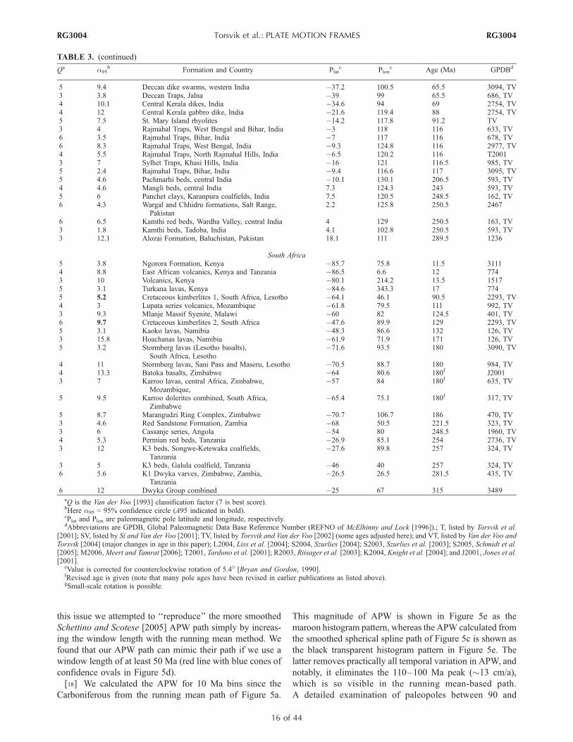
this issue we attempted to ‘‘reproduce’’ the more smoothedSchettino and Scotese [2005] APW path simply by increas-ing the window length with the running mean method. Wefound that our APW path can mimic their path if we use awindow length of at least 50 Ma (red line with blue cones ofconfidence ovals in Figure 5d).[18] We calculated the APW for 10 Ma bins since the
Carboniferous from the running mean path of Figure 5a.
This magnitude of APW is shown in Figure 5e as themaroon histogram pattern, whereas the APW calculated fromthe smoothed spherical spline path of Figure 5c is shown asthe black transparent histogram pattern in Figure 5e. Thelatter removes practically all temporal variation in APW, andnotably, it eliminates the 110–100 Ma peak (!13 cm/a),which is so visible in the running mean-based path.A detailed examination of paleopoles between 90 and
Qa a95b Formation and Country Plat
c Plonc Age (Ma) GPDBd
5 9.4 Deccan dike swarms, western India "37.2 100.5 65.5 3094, TV3 3.8 Deccan Traps, Jalna "39 99 65.5 686, TV4 10.1 Central Kerala dikes, India "34.6 94 69 2754, TV4 12 Central Kerala gabbro dike, India "21.6 119.4 88 2754, TV5 7.5 St. Mary Island rhyolites "14.2 117.8 91.2 TV3 4 Rajmahal Traps, West Bengal and Bihar, India "3 118 116 633, TV6 3.5 Rajmahal Traps, Bihar, India "7 117 116 678, TV6 8.3 Rajmahal Traps, West Bengal, India "9.3 124.8 116 2977, TV4 5.5 Rajmahal Traps, North Rajmahal Hills, India "6.5 120.2 116 T20013 7 Sylhet Traps, Khasi Hills, India "16 121 116.5 985, TV5 2.4 Rajmahal Traps, Bihar, India "9.4 116.6 117 3095, TV5 4.6 Pachmarhi beds, central India "10.1 130.1 206.5 593, TV4 4.6 Mangli beds, central India 7.3 124.3 243 593, TV5 6 Panchet clays, Karanpura coalfields, India 7.5 120.5 248.5 162, TV6 4.3 Wargal and Chhidru formations, Salt Range,
Pakistan2.2 125.8 250.5 2467
6 6.5 Kamthi red beds, Wardha Valley, central India 4 129 250.5 163, TV3 1.8 Kamthi beds, Tadoba, India 4.1 102.8 250.5 593, TV3 12.1 Alozai Formation, Baluchistan, Pakistan 18.1 111 289.5 1236
South Africa5 3.8 Ngorora Formation, Kenya "85.7 75.8 11.5 31114 8.8 East African volcanics, Kenya and Tanzania "86.5 6.6 12 7743 10 Volcanics, Kenya "80.1 214.2 13.5 15175 3.1 Turkana lavas, Kenya "84.6 343.3 17 7745 5.2 Cretaceous kimberlites 1, South Africa, Lesotho "64.1 46.1 90.5 2293, TV4 3 Lupata series volcanics, Mozambique "61.8 79.5 111 992, TV3 9.3 Mlanje Massif Syenite, Malawi "60 82 124.5 401, TV6 9.7 Cretaceous kimberlites 2, South Africa "47.6 89.9 129 2293, TV5 3.1 Kaoko lavas, Namibia "48.3 86.6 132 126, TV3 15.8 Hoachanas lavas, Namibia "61.9 71.9 171 126, TV5 3.2 Stormberg lavas (Lesotho basalts),
South Africa, Lesotho"71.6 93.5 180 3090, TV
4 11 Stormberg lavas, Sani Pass and Maseru, Lesotho "70.5 88.7 180 984, TV4 13.3 Batoka basalts, Zimbabwe "64 80.6 180f J20013 7 Karroo lavas, central Africa, Zimbabwe,
Mozambique,"57 84 180f 635, TV
5 9.5 Karroo dolerites combined, South Africa,Zimbabwe
"65.4 75.1 180f 317, TV
5 8.7 Marangudzi Ring Complex, Zimbabwe "70.7 106.7 186 470, TV3 4.6 Red Sandstone Formation, Zambia "68 50.5 221.5 323, TV3 6 Cassanje series, Angola "54 80 248.5 1960, TV4 5.3 Permian red beds, Tanzania "26.9 85.1 254 2736, TV3 12 K3 beds, Songwe-Ketewaka coalfields,
Tanzania"27.6 89.8 257 324, TV
3 5 K3 beds, Galula coalfield, Tanzania "46 40 257 324, TV6 5.6 K1 Dwyka varves, Zimbabwe, Zambia,
Tanzania"26.5 26.5 281.5 435, TV
6 12 Dwyka Group combined "25 67 315 3489aQ is the Van der Voo [1993] classification factor (7 is best score).bHere a95 = 95% confidence circle (A95 indicated in bold).cPlat and Plon are paleomagnetic pole latitude and longitude, respectively.dAbbreviations are GPDB, Global Paleomagnetic Data Base Reference Number (REFNO of McElhinny and Lock [1996]).; T, listed by Torsvik et al.
[2001]; SV, listed by Si and Van der Voo [2001]; TV, listed by Torsvik and Van der Voo [2002] (some ages adjusted here); and VT, listed by Van der Voo andTorsvik [2004] (major changes in age in this paper); L2004, Liss et al. [2004]; S2004, Szurlies [2004]; S2003, Szurlies et al. [2003]; S2005, Schmidt et al.[2005]; M2006,Meert and Tamrat [2006]; T2001, Tarduno et al. [2001]; R2003, Riisager et al. [2003]; K2004, Knight et al. [2004]; and J2001, Jones et al.[2001].
eValue is corrected for counterclockwise rotation of 5.4! [Bryan and Gordon, 1990].fRevised age is given (note that many pole ages have been revised in earlier publications as listed above).gSmall-scale rotation is possible.
TABLE 3. (continued)
RG3004 Torsvik et al.: PLATE MOTION FRAMES
16 of 44
RG3004

120 Ma (as used to calculate the running mean path andshown in Figure 6a) clearly illustrates that this peak is real(even when smoothed because of the 10 Ma movingwindow overlap) because there is indeed a ‘‘systematic’’progression of the Cretaceous poles for this interval. Hencethe spherical spline path has smoothed away this importantshort-time APW feature.
3.4. Plate Motion Chains and the Pangea Enigma
[19] Different Euler rotations for relative plate motionscan produce significant differences between global APWpaths. Most of our Euler rotations (Tables 1 and 2) differfrom those of Besse and Courtillot [2002], where finite(Euler) rotations were largely recomputed from the Mulleret al. [1993] model described in section 4. Conversely,many Euler rotations of Schettino and Scotese [2005] werecalculated by inversion of the digital ocean seafloor grid ofMuller et al. [1997]. Different choices will naturally affectthe resultant global APW path. Moreover, we have extendedour APW path back to 320 Ma, which introduces someadditional enigmas.
[20] Paleomagnetic poles are calculated under the routineassumption that the time-averaged geomagnetic field is thatof a geocentric axial dipole. However, Van der Voo andTorsvik [2001] have suggested that nondipole field contri-butions may have persisted through significant periods ofEarth history. Most Earth scientists agree that before theonset of breakup, the Jurassic ‘‘Pangea A’’ reconstruction isthe correct one, in which NW Africa is located adjacent tothe Atlantic margin of North America (Figure 3a). ForPermian times, however, the paleomagnetic poles do notagree with the Pangea A fit of Figure 3a, as can be seen byexamining the discrepancy between the poles from Gond-wana and those for Laurussia in Figures 4b and 6b. Toreconcile the paleomagnetic misfit, one has the option of(1) modifying the Pangea A reconstruction or (2) dismissingmuch of the database as contaminated by later magneticoverprints or (3) arguing that the mean pole positions areimprecise because of rock magnetic recording problems,such as those caused by sedimentary inclination shallowing[e.g., Kodama, 1997; Rochette and Vandamme, 2001;Torsvik and Van der Voo, 2002; Kent and Tauxe, 2005]. Afourth solution is to hypothesize significant octupole fieldcontributions, in which case the Pangea misfit is caused byinferring a too far northerly position of Gondwana from thegeocentric axial dipole hypothesis, as well as a too far southposition for Laurussia [Van der Voo and Torsvik, 2001,2004; Torsvik and Van der Voo, 2002]. Latitudinal errorscaused by 5–10% octupole field contributions are compa-rable to inclination shallowing effects in sediments. All fourof these explanations have been presented in previouspublications [see Van der Voo, 1993; Muttoni et al., 2003;Irving, 2004; Van der Voo and Torsvik, 2004, and referencestherein]. The largest misfit is seen at 250 Ma (Figure 6b),likely because the data are indeed not very reliable for thisinterval, as argued by Muttoni et al. [2003].[21] In general, the number of poles from Laurussia is
larger (and, on average, of higher data quality) than simi-larly aged poles from Gondwana, and they will thereforebias the global path. Since the incorporation of nondipolecontributions is controversial, we opted in this paper to onlyanalyze geocentric axial dipole–based APW paths. How-ever, we should mention that the debate about the variousPangea reconstructions has not subsided [see Irving, 2004]and that different Pangea fits labeled A2 and B (or lesscommonly C or D) remain favored even in recent literature.Since nondipole field contributions remain an open possi-bility, we refer to Table 4 (see column labeled SAFR**) fora comparison of our geocentric axial dipole–based APWpath with one that incorporates time-dependent nondipolefields (0–17.5% octupole contributions) [Torsvik and Vander Voo, 2002]. On average, however, this alternative pathdiffers by only 2.0! ± 1.3! (great circle distance betweenpoles of same mean age).
3.5. Paleomagnetic Euler Pole Analysis
[22] Movements of continents, APW paths (in the ab-sence of true polar wander), tracks of hot spots (if fixed tothe mantle), and ocean fracture zones all should represent
Figure 4. The 419 paleomagnetic results selected for theanalysis of this paper (Table 3) and plotted as south poles inSouth African coordinates, using the rotation parameterslisted in Tables 1 and 2. (a) Poles <200 Ma and (b) poles>200 Ma and <320 Ma. Note that many ‘‘Gondwana’’ southpoles in Figure 4b plot at significantly more easterlylongitudes for Late Permian and Triassic times. Thenumbers next to these Gondwana poles are their ages (Ma).
RG3004 Torsvik et al.: PLATE MOTION FRAMES
17 of 44
RG3004

Figure 5. (a) Global running mean (RM) apparent polar wander (APW) path (thick black line with blueconfidence circles, A95) in South African coordinates, with ages in million years. This path is generatedwith a 20 Ma moving window, incremented at 10 Ma intervals. The red line is a spherical smoothedspline path (smoothing parameter is 1000) [see Torsvik et al., 1996; Jupp and Kent, 1987]. The splinepath uses raw data (70–210 Ma), which are weighted by their Q factor; see text for details. (b) Greatcircle distances (GCD) between the running mean path of Figure 5a and the APW paths of Schettino andScotese [2005] (SS2005) and Besse and Courtillot [2002] (BC2002). The SS2005 path comparison isshown together with the errors in our RM path. (c) A spherical, smoothed spline path (smoothingparameter is 700) based on a running mean path (without data overlap, just binned) and with weighting ofinput poles according to A95. The A95 values for the output spline path will increase with increasedsmoothing because the spline is farther and farther displaced from the real input poles. This heavilysmoothed spline path (red) is compared with the SS2005 APW path (blue). No errors were provided in theSS2005 model. (d) A running mean APW path, which uses extreme smoothing (window length of 50 Ma),shown together with the BC2002 path with light green–shaded A95 ovals. (e) Calculated APW rates (for10 Ma intervals) using our global RM path of Figure 5a and the smoothed spline path of Figure 5c.
RG3004 Torsvik et al.: PLATE MOTION FRAMES
18 of 44
RG3004
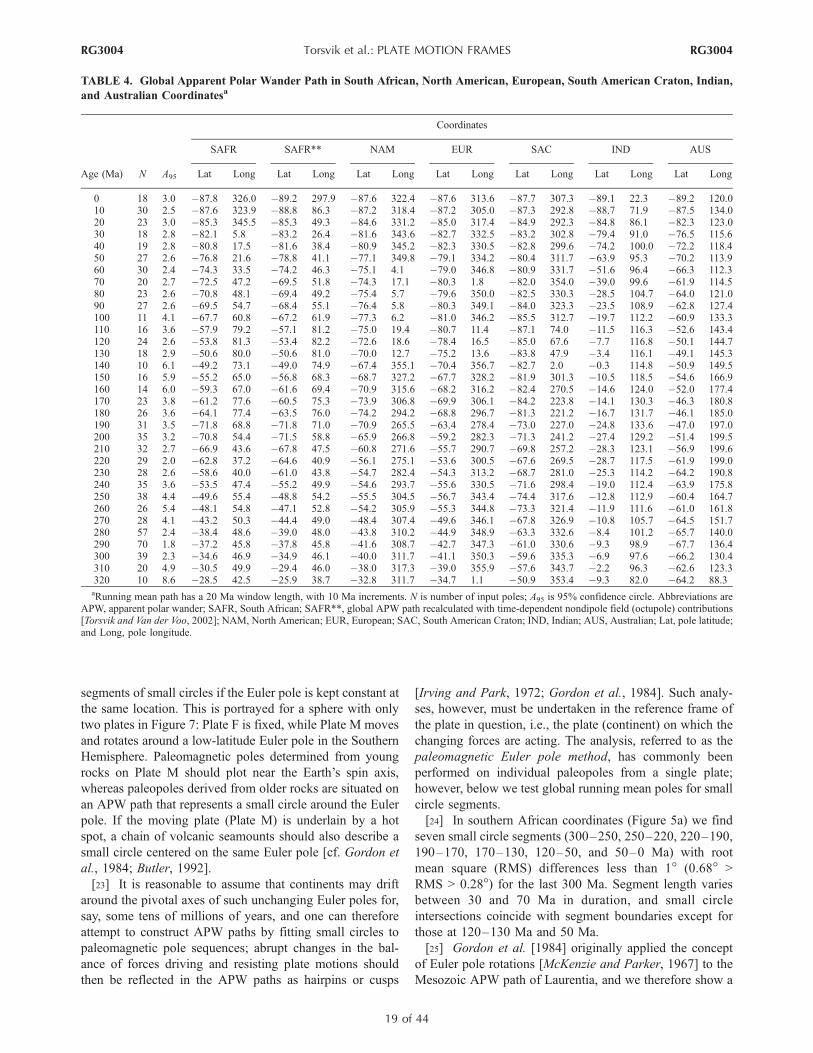
segments of small circles if the Euler pole is kept constant atthe same location. This is portrayed for a sphere with onlytwo plates in Figure 7: Plate F is fixed, while Plate M movesand rotates around a low-latitude Euler pole in the SouthernHemisphere. Paleomagnetic poles determined from youngrocks on Plate M should plot near the Earth’s spin axis,whereas paleopoles derived from older rocks are situated onan APW path that represents a small circle around the Eulerpole. If the moving plate (Plate M) is underlain by a hotspot, a chain of volcanic seamounts should also describe asmall circle centered on the same Euler pole [cf. Gordon etal., 1984; Butler, 1992].[23] It is reasonable to assume that continents may drift
around the pivotal axes of such unchanging Euler poles for,say, some tens of millions of years, and one can thereforeattempt to construct APW paths by fitting small circles topaleomagnetic pole sequences; abrupt changes in the bal-ance of forces driving and resisting plate motions shouldthen be reflected in the APW paths as hairpins or cusps
[Irving and Park, 1972; Gordon et al., 1984]. Such analy-ses, however, must be undertaken in the reference frame ofthe plate in question, i.e., the plate (continent) on which thechanging forces are acting. The analysis, referred to as thepaleomagnetic Euler pole method, has commonly beenperformed on individual paleopoles from a single plate;however, below we test global running mean poles for smallcircle segments.[24] In southern African coordinates (Figure 5a) we find
seven small circle segments (300–250, 250–220, 220–190,190–170, 170–130, 120–50, and 50–0 Ma) with rootmean square (RMS) differences less than 1! (0.68! >RMS > 0.28!) for the last 300 Ma. Segment length variesbetween 30 and 70 Ma in duration, and small circleintersections coincide with segment boundaries except forthose at 120–130 Ma and 50 Ma.[25] Gordon et al. [1984] originally applied the concept
of Euler pole rotations [McKenzie and Parker, 1967] to theMesozoic APW path of Laurentia, and we therefore show a
TABLE 4. Global Apparent Polar Wander Path in South African, North American, European, South American Craton, Indian,and Australian Coordinatesa
Age (Ma) N A95
Coordinates
SAFR SAFR** NAM EUR SAC IND AUS
Lat Long Lat Long Lat Long Lat Long Lat Long Lat Long Lat Long
0 18 3.0 "87.8 326.0 "89.2 297.9 "87.6 322.4 "87.6 313.6 "87.7 307.3 "89.1 22.3 "89.2 120.010 30 2.5 "87.6 323.9 "88.8 86.3 "87.2 318.4 "87.2 305.0 "87.3 292.8 "88.7 71.9 "87.5 134.020 23 3.0 "85.3 345.5 "85.3 49.3 "84.6 331.2 "85.0 317.4 "84.9 292.3 "84.8 86.1 "82.3 123.030 18 2.8 "82.1 5.8 "83.2 26.4 "81.6 343.6 "82.7 332.5 "83.2 302.8 "79.4 91.0 "76.5 115.640 19 2.8 "80.8 17.5 "81.6 38.4 "80.9 345.2 "82.3 330.5 "82.8 299.6 "74.2 100.0 "72.2 118.450 27 2.6 "76.8 21.6 "78.8 41.1 "77.1 349.8 "79.1 334.2 "80.4 311.7 "63.9 95.3 "70.2 113.960 30 2.4 "74.3 33.5 "74.2 46.3 "75.1 4.1 "79.0 346.8 "80.9 331.7 "51.6 96.4 "66.3 112.370 20 2.7 "72.5 47.2 "69.5 51.8 "74.3 17.1 "80.3 1.8 "82.0 354.0 "39.0 99.6 "61.9 114.580 23 2.6 "70.8 48.1 "69.4 49.2 "75.4 5.7 "79.6 350.0 "82.5 330.3 "28.5 104.7 "64.0 121.090 27 2.6 "69.5 54.7 "68.4 55.1 "76.4 5.8 "80.3 349.1 "84.0 323.3 "23.5 108.9 "62.8 127.4100 11 4.1 "67.7 60.8 "67.2 61.9 "77.3 6.2 "81.0 346.2 "85.5 312.7 "19.7 112.2 "60.9 133.3110 16 3.6 "57.9 79.2 "57.1 81.2 "75.0 19.4 "80.7 11.4 "87.1 74.0 "11.5 116.3 "52.6 143.4120 24 2.6 "53.8 81.3 "53.4 82.2 "72.6 18.6 "78.4 16.5 "85.0 67.6 "7.7 116.8 "50.1 144.7130 18 2.9 "50.6 80.0 "50.6 81.0 "70.0 12.7 "75.2 13.6 "83.8 47.9 "3.4 116.1 "49.1 145.3140 10 6.1 "49.2 73.1 "49.0 74.9 "67.4 355.1 "70.4 356.7 "82.7 2.0 "0.3 114.8 "50.9 149.5150 16 5.9 "55.2 65.0 "56.8 68.3 "68.7 327.2 "67.7 328.2 "81.9 301.3 "10.5 118.5 "54.6 166.9160 14 6.0 "59.3 67.0 "61.6 69.4 "70.9 315.6 "68.2 316.2 "82.4 270.5 "14.6 124.0 "52.0 177.4170 23 3.8 "61.2 77.6 "60.5 75.3 "73.9 306.8 "69.9 306.1 "84.2 223.8 "14.1 130.3 "46.3 180.8180 26 3.6 "64.1 77.4 "63.5 76.0 "74.2 294.2 "68.8 296.7 "81.3 221.2 "16.7 131.7 "46.1 185.0190 31 3.5 "71.8 68.8 "71.8 71.0 "70.9 265.5 "63.4 278.4 "73.0 227.0 "24.8 133.6 "47.0 197.0200 35 3.2 "70.8 54.4 "71.5 58.8 "65.9 266.8 "59.2 282.3 "71.3 241.2 "27.4 129.2 "51.4 199.5210 32 2.7 "66.9 43.6 "67.8 47.5 "60.8 271.6 "55.7 290.7 "69.8 257.2 "28.3 123.1 "56.9 199.6220 29 2.0 "62.8 37.2 "64.6 40.9 "56.1 275.1 "53.6 300.5 "67.6 269.5 "28.7 117.5 "61.9 199.0230 28 2.6 "58.6 40.0 "61.0 43.8 "54.7 282.4 "54.3 313.2 "68.7 281.0 "25.3 114.2 "64.2 190.8240 35 3.6 "53.5 47.4 "55.2 49.9 "54.6 293.7 "55.6 330.5 "71.6 298.4 "19.0 112.4 "63.9 175.8250 38 4.4 "49.6 55.4 "48.8 54.2 "55.5 304.5 "56.7 343.4 "74.4 317.6 "12.8 112.9 "60.4 164.7260 26 5.4 "48.1 54.8 "47.1 52.8 "54.2 305.9 "55.3 344.8 "73.3 321.4 "11.9 111.6 "61.0 161.8270 28 4.1 "43.2 50.3 "44.4 49.0 "48.4 307.4 "49.6 346.1 "67.8 326.9 "10.8 105.7 "64.5 151.7280 57 2.4 "38.4 48.6 "39.0 48.0 "43.8 310.2 "44.9 348.9 "63.3 332.6 "8.4 101.2 "65.7 140.0290 70 1.8 "37.2 45.8 "37.8 45.8 "41.6 308.7 "42.7 347.3 "61.0 330.6 "9.3 98.9 "67.7 136.4300 39 2.3 "34.6 46.9 "34.9 46.1 "40.0 311.7 "41.1 350.3 "59.6 335.3 "6.9 97.6 "66.2 130.4310 20 4.9 "30.5 49.9 "29.4 46.0 "38.0 317.3 "39.0 355.9 "57.6 343.7 "2.2 96.3 "62.6 123.3320 10 8.6 "28.5 42.5 "25.9 38.7 "32.8 311.7 "34.7 1.1 "50.9 353.4 "9.3 82.0 "64.2 88.3aRunning mean path has a 20 Ma window length, with 10 Ma increments. N is number of input poles; A95 is 95% confidence circle. Abbreviations are
APW, apparent polar wander; SAFR, South African; SAFR**, global APW path recalculated with time-dependent nondipole field (octupole) contributions[Torsvik and Van der Voo, 2002]; NAM, North American; EUR, European; SAC, South American Craton; IND, Indian; AUS, Australian; Lat, pole latitude;and Long, pole longitude.
RG3004 Torsvik et al.: PLATE MOTION FRAMES
19 of 44
RG3004
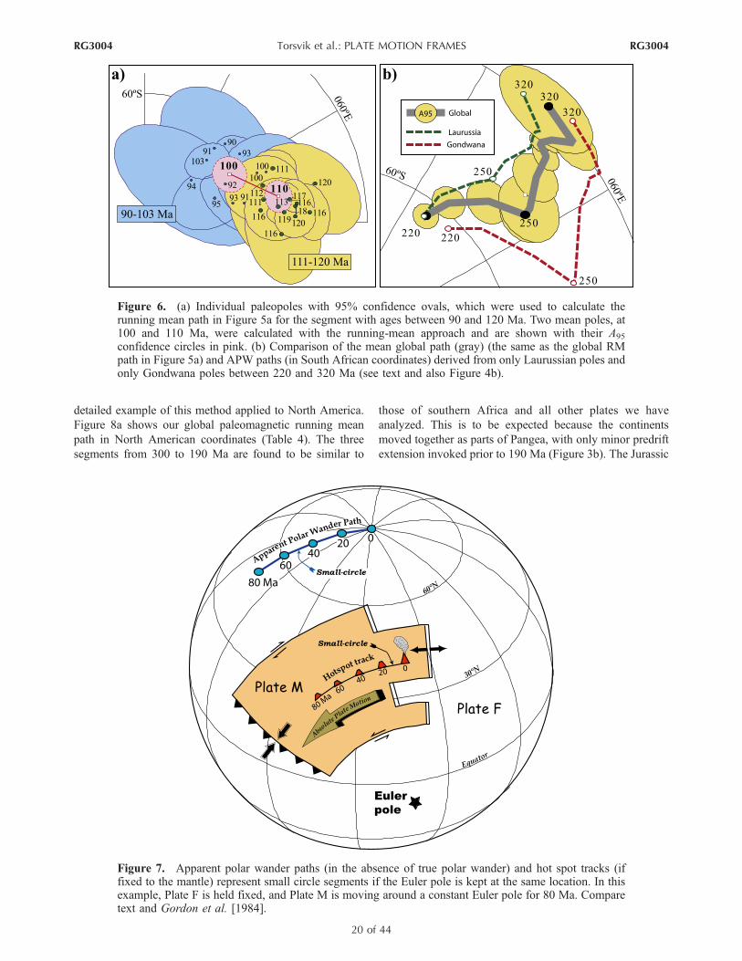
detailed example of this method applied to North America.Figure 8a shows our global paleomagnetic running meanpath in North American coordinates (Table 4). The threesegments from 300 to 190 Ma are found to be similar to
those of southern Africa and all other plates we haveanalyzed. This is to be expected because the continentsmoved together as parts of Pangea, with only minor predriftextension invoked prior to 190 Ma (Figure 3b). The Jurassic
Figure 7. Apparent polar wander paths (in the absence of true polar wander) and hot spot tracks (iffixed to the mantle) represent small circle segments if the Euler pole is kept at the same location. In thisexample, Plate F is held fixed, and Plate M is moving around a constant Euler pole for 80 Ma. Comparetext and Gordon et al. [1984].
Figure 6. (a) Individual paleopoles with 95% confidence ovals, which were used to calculate therunning mean path in Figure 5a for the segment with ages between 90 and 120 Ma. Two mean poles, at100 and 110 Ma, were calculated with the running-mean approach and are shown with their A95
confidence circles in pink. (b) Comparison of the mean global path (gray) (the same as the global RMpath in Figure 5a) and APW paths (in South African coordinates) derived from only Laurussian poles andonly Gondwana poles between 220 and 320 Ma (see text and also Figure 4b).
RG3004 Torsvik et al.: PLATE MOTION FRAMES
20 of 44
RG3004

section, however, differs substantially; the abrupt 170 Macusp seen for southern Africa (Figure 5a) is not present.Instead, there is a change in trajectory at 150 Ma where anintersection occurs between the 190–150 and the 150–130 Ma segments, but there is no trace of a distinct cusp.Similarly for southern Africa, we can fit small circles to thesegments of 120–50 Ma (RMS = 0.81!) and 50–0 Ma(RMS = 0.23!), but the magnitude of Laurentian APW
between 120 and 50 Ma (0.13!/Ma) is much less than that ofsouthern Africa (0.45!/Ma). Our analysis is very differentfrom any earlier paleomagnetic Euler pole analysis becausewe use global running mean poles and not just NorthAmerican poles [see Beck and Housen, 2003], which showlower pole latitudes during the Middle-Late Jurassic thanthose predicted from a global model. We illustrate this inFigure 8a where the red dashed line represents a running
Figure 8. (a) Global apparent polar wander (APW) path, the same as in Figure 5a for the last 300 Ma,but shown in North American coordinates and fitted by seven small circle segments (black solid lines)discussed in the text. The red dashed line represents a running mean path exclusively based on NorthAmerican poles. (b) Zoomed-in segment of the 50–120 Ma mean poles in order to examine poles duringthe North American Cretaceous stillstand. (c) Global APW rate in North American coordinates. Noticethat the 110–100 Ma peak seen in southern African coordinates is not seen in North Americancoordinates, as in the latter it represents what has been called the ‘‘Cretaceous stillstand.’’ Encircledletters, T1, T2, J1, J2, C, and T, are kinks or cusp intersections seen in Figure 8a, where they are markedby white arrows. Calculated (d) north–south drift and (e) angular rotation of North America based on theglobal running mean path for a specific location (45!N, 260!E).
RG3004 Torsvik et al.: PLATE MOTION FRAMES
21 of 44
RG3004

mean APW path, calculated exclusively from North Amer-ican poles (Table 3). In this purely North American runningmean path the global 250 Ma cusp has vanished (no longerinfluenced by Gondwana poles, see Figure 6b); the 220 Maknickpoint is deteriorating (the segments being replaced bya single small circle from 270 to 190 Ma, RMS = 0.58!),whereas the 190, 120, and 50 Ma cusps are recognized, justas they were in the global running mean path. However, theMiddle-Late Jurassic section differs markedly, with a knick-point near 160 Ma, located at lower latitude. This is relevantto the debate about the reliability of the Laurentian JurassicAPW segment [e.g., Ekstrand and Butler, 1989; Witte andKent, 1990; Van Fossen and Kent, 1990; Van der Voo, 1992;Courtillot et al., 1994].[26] On the basis of North American data alone and
different pole selection criteria, Beck and Housen [2003]identified three small circle tracks (245–200, 200–160, and160–125 Ma) and their two intersections (or cusps, both arepronounced), named J1 and J2 (following Gordon et al.[1984]). Using this nomenclature but on the basis of ourglobal running mean path data, J1 (!190 Ma in our globalanalysis) occurs shortly before seafloor spreading began inthe central Atlantic (rift to drift and the first real breakupphase of Pangea) and !10 Ma after eruption of the CentralAtlantic Magmatic Province. This J1 cusp at 190 Ma isassociated with the second biggest burst in APW (Figure 8c),linked to a peak in angular rotation that initiated a prolongedperiod of clockwise rotation of !50 Ma duration. Con-versely, J2 (!150 Ma) coincides with local high seafloorspreading rates in the central Atlantic (Figure 3b) andoccurs shortly before a northward velocity increase thatcoincides with the highest amount of APW for NorthAmerica during the entire Mesozoic (Figures 8c and 8d).The Cretaceous is marked by decreasing APW, and theCretaceous cusp at !125 Ma (labeled C in Figures 8c–8eand Figure 3b) marks the beginning of the so-called NorthAmerican Cretaceous stillstand that lasted until !70 Ma asjudged from our global running mean path (Figures 8b and8c). This apparent stillstand ended when seafloor spreading(rift to drift) occurred in the Labrador Sea between NorthAmerica and Greenland at!67Ma (see Table 1 and Figure 3b).The C cusp is associated with the onset of the highestseafloor spreading peak in the central Atlantic (Figure 3b).In an ‘‘absolute’’ sense we argue that the North AmericanCretaceous stillstand is only apparent and that it was causedby a dominating component of paleo-east-to-west drift(section 7). Finally, a Tertiary cusp (labeled T at 50 Ma inFigures 3b and 8c–8e) at around 50 Ma is linked to seafloorspreading in the North Atlantic and the accompanyingwestward drift of the North American plate. The oldercusps (denoted T1 and T2 in Figures 8c–8e and 3b) willbe discussed in section 8.2.
4. AFRICAN FIXED HOT SPOT FRAME
[27] Wilson [1963] first suggested that linear chains ofseamounts and volcanoes, which display age progression,are caused by focused spots of melting in the mantle, termed
‘‘hot spots.’’ Morgan [1971] proposed that hot spots may becaused by mantle plumes upwelling from the lower mantle,which in his model remain fixed relative to each other overgeologically long periods of time (‘‘fixed hot spot hypoth-esis’’). During the past 40 years a multitude of marinegeophysical data and isotope ages of seamounts fromvolcanic hot spot tracks have been collected, allowingreconstructions of plate motions relative to hot spots sincethe Cretaceous.[28] Early attempts to reconstruct all major tectonic plates
with respect to one collective set of hot spots (presumedfixed relative to each other) led to the realization thatmodels constructed for Pacific plate motions over hot spotscould not be reconciled with the motions over the hot spotsin the African–Indian Ocean domain for the last 80 Ma[Duncan, 1981; Morgan, 1981]. Subsequently, evidence hasaccumulated that hot spots underlying the Pacific cannothave remained fixed relative to the Atlantic-Indian hot spots[Molnar and Stock, 1987; Tarduno and Gee, 1995; Tardunoand Cottrell, 1997; DiVenere and Kent, 1999; Torsvik et al.,2002; Tarduno et al., 2003]. However, hot spots within theAtlantic-Indian domain appear to have moved much lessdramatically relative to each other. On the basis of thisinference, Muller et al. [1993] used an interactive techniqueto derive a ‘‘best fit’’ model in a qualitative sense formotions of the major plates in the Atlantic-Indian domainrelative to hot spot tracks with a clear age progression.[29] Even though this model is widely used, it has some
well-recognized shortcomings: the Late Tertiary portion ofthis model was not well constrained by radiometric agesbecause of the lack of published age dates for the post–30 Ma portion of most hot spot tracks. For reconstructiontimes predating 80Ma, the only available hot spot tracks witha reasonably well known age progression in the Atlantic-Indian oceans are those of the New England seamount chain(linked to the Great Meteor hot spot) and the Walvis Ridge/Rio Grande Rise (linked to the Tristan hot spot, Figure 9),both in the Atlantic Ocean. Therefore, the absolute motionof the Indian, Australian, and Antarctic plates relative to themantle has to be computed solely based on plate motionchains for these times. However, when the Muller et al.[1993] model was constructed, pre–80 Ma relative platemotions in the Indian Ocean were poorly known because ofa lack of data in crucial areas, in particular offshoreAntarctica in the Enderby Basin and south of the KerguelenPlateau. This has recently improved as a sequence ofMesozoic magnetic anomalies was mapped and modeledin the Enderby Basin, starting at about 130 Ma [Gaina etal., 2003, 2007]. The Muller et al. [1993] model was basedon the assumption of post–120 Ma breakup between Indiaand Madagascar, placing India too far north from 130 toabout 90 Ma. Disagreements between the hot spot andpaleomagnetic reference frames have been documented forIndia [Muller et al., 1994; Torsvik et al., 1998] and forAustralia [Idnurm, 1985], suggesting either an incorrectrelative plate motion model, relative motion between hotspots through time, or true polar wander or any combinationof these three issues. As an example, paleopoles for India
RG3004 Torsvik et al.: PLATE MOTION FRAMES
22 of 44
RG3004

from the Rajmahal Traps (Table 3) result in a paleolatitudeof the traps at their time of formation (!116 Ma) at 47!S,whereas the Muller et al. [1993] model places them at about40!S.[30] A comparison of mid-Cretaceous (122–80 Ma)
paleolatitudes of North America and Africa from paleomag-netic data with those from hot spot tracks [Van Fossen andKent, 1992] provided evidence for an 11!–13! discrepancy,suggesting that Atlantic hot spots likely did not remain fixedrelative to the Earth’s spin axis before 80 Ma. With ourmore recent analyses using a different time interval andcompared to the Muller et al. [1993] model, we find that thehot spots moved southward as much as 18! between 100and 130 Ma [Torsvik et al., 2002]. Others argue that thisapparent southward movement was caused by true polarwander (TPW) [see Prevot et al., 2000; Camps et al., 2002;Tarduno and Smirnov, 2002].[31] The Muller et al. [1993] plate motion model results
in a relatively sharp turn in plate motion directions (e.g., ofAustralia and Antarctica) relative to the mantle at about80 Ma, which originates from the bend between the New
England seamount chain and the Corner seamounts atroughly 80 Ma in the central Atlantic. An equivalent bendin fracture zones is not found in either the Pacific or Indianoceans. Bends in hot spot tracks, which are not seen inrelative motions of the plates involved, are likely because oftime-varying velocities of local mantle (hot spot) motionrelative to the mean mantle, as has been suggested as havingcaused the bend in the Hawaiian-Emperor chain [Norton,1995; Tarduno and Cottrell, 1997]. It follows that thecentral Atlantic bend may be due to a slowdown insouthward motion of the mantle underlying at least theAtlantic Ocean and its bordering continents at around 80 Maand that fixed hot spot models therefore need to be replacedby models that take into account the motion of hot spots in aconvecting mantle.[32] The plate motion model used by Muller et al. [1993]
was based on the timescales of Berggren et al. [1985] andKent and Gradstein [1985]. In order to compare Muller etal. [1993] with more recent models for the purpose of thispaper, we first need to translate it to more recent timescales[Cande and Kent, 1995; Gradstein et al., 1994]. This
Figure 9. Walvis Ridge (linked to the Tristan hot spot at 38!S, 11!W) analyzed in a comparison of theAfrican fixed hot spot model of Muller et al. [1993] (light blue circles) and the revised fixed hot spotmodel of this study (red circles), at 10 Ma interpolated intervals, showing that the differences arerelatively small. The marine gravity data have been taken from Sandwell and Smith [1997].
RG3004 Torsvik et al.: PLATE MOTION FRAMES
23 of 44
RG3004
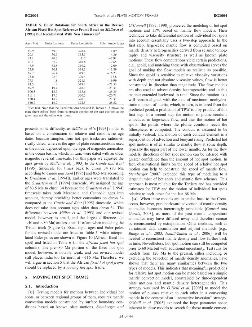
presents some difficulty, as Muller et al.’s [1993] model isbased on a combination of relative and radiometric agedates, because samples from hot spot tracks are radiomet-rically dated, whereas the ages of plate reconstructions usedin the model depended upon the ages of magnetic anomaliesin the ocean basins, which, in turn, were dated with an oldermagnetic reversal timescale. For this paper we adjusted theages given by Muller et al. [1993] to the Cande and Kent[1995] timescale for times back to chron 34 (83 Maaccording to Cande and Kent [1995] and 83.5 Ma accordingto Gradstein et al. [1994]). Earlier ages were translated tothe Gradstein et al. [1994] timescale. We assigned the ageof 83.5 Ma to chron 34 because the Gradstein et al. [1994]timescale takes both Mesozoic and Cenozoic ages intoaccount, thereby providing better constraints on chron 34compared to the Cande and Kent [1995] timescale, whichdoes not take into account ages older than chron 34. Thedifference between Muller et al. [1993] and our revisedmodel, however, is small, and the largest differences (at!40 and !80 Ma) are less than 1! of arc when modeling theTristan track (Figure 9). Exact input ages and Euler polesfor the revised model are listed in Table 5, while interpo-lated Euler poles are shown in Figure 10 (African fixed hotspot) and listed in Table 6 (in the African fixed hot spotcolumn). The pre–80 Ma portion of the fixed hot spotmodel, however, is notably weak, and our revised modelstill places India too far north at !116 Ma. Therefore, wewill argue in section 5 that the African fixed hot spot frameshould be replaced by a moving hot spot frame.
5. MOVING HOT SPOT FRAMES
5.1. Introduction
[33] Testing models for motions between individual hotspots, or between regional groups of them, requires mantleconvection models constrained by surface boundary con-ditions based on known plate motions. Steinberger and
O’Connell [1997, 1998] pioneered the modeling of hot spotmotions and TPW based on mantle flow models. Theirtechnique to take differential motion of individual hot spotsinto account essentially uses a two-step approach: In thefirst step, large-scale mantle flow is computed based onmantle density heterogeneities derived from seismic tomog-raphy and viscosity structure as well as known platemotions. These flow computations yield certain predictions,e.g., geoid, and matching these with observations serves thegoal of making the flow models as realistic as possible.Since the geoid is sensitive to relative viscosity variationswith depth and not absolute viscosity values, flow is betterconstrained in direction than magnitude. The flow modelsare also used to advect density heterogeneities and in thismanner extended backward in time. Since the rotation axiswill remain aligned with the axis of maximum nonhydro-static moment of inertia, which, in turn, is inferred from thepredicted geoid, a prediction of TPW is a by-product of thisfirst step. In a second step the motion of plume conduitsembedded in large-scale flow, and thus the motion of hotspots, the points where the plume conduits reach thelithosphere, is computed. The conduit is assumed to beinitially vertical, and motion of each conduit element is asuperposition of advection and buoyant rising. Predicted hotspot motion is often similar to mantle flow at some depth,typically the upper part of the lower mantle. As for the flowmodels, directions of hot spot motion can be inferred withgreater confidence than the amount of hot spot motion. Infact, observational limits on the speed of relative hot spotmotion can help to constrain the speed of mantle flow.Steinberger [2000] extended this type of modeling to alarger number of hot spots and mantle flow schemes. Thisapproach is most reliable for the Tertiary and has providedestimates for TPW and the motion of individual hot spotsrelative to each other for the last 68 Ma.[34] When these models are extended back to the Creta-
ceous, however, pure backward advection of mantle densityanomalies becomes increasingly unreliable [Conrad andGurnis, 2003], as more of the past mantle temperatureanomalies may have diffused away and therefore cannotbe reconstructed by extrapolation. Other methods, such asvariational data assimilation and adjoint methods [e.g.,Bunge et al., 2003; Ismail-Zadeh et al., 2006], will beneeded to reconstruct mantle density and flow further backin time. Nevertheless, hot spot motion can still be computedprior to 68 Ma but with additional uncertainty. Test runs formodels from 120 Ma to the present, either including orexcluding the advection of mantle density anomalies, haveshown that there are many similarities between the twotypes of models. This indicates that meaningful predictionsfor relative hot spot motion can be made based on a simplemantle convection model, constrained by time-dependentplate motions and mantle density heterogeneities. Thisstrategy was used by O’Neill et al. [2005] to model themotion of plumes relative to each other in a convectingmantle in the context of an ‘‘interactive inversion’’ strategy.O’Neill et al. [2005] explored the large parameter spaceinherent in these models to search for those mantle convec-
TABLE 5. Euler Rotations for South Africa in the RevisedAfrican Fixed Hot Spot Reference Frame Based onMuller et al.[1993] But Recalculated With New Timescalesa
Age (Ma) Euler Latitude Euler Longitude Euler Angle (deg)
10.9 59.3 328.4 "1.8920.1 50.9 315.5 "4.3633.1 40.3 317 "7.9140.1 37.7 318.8 "9.6547.9 32.8 319.2 "12.0955.9 30.1 318.3 "13.8967.7 26.4 319.1 "16.2373.0 22.3 320.4 "17.879.1 18 321.1 "19.9983.5 19 319.1 "21.5389.9 19.4 318.1 "23.31100.5 18.9 318.6 "25.35111.1 17.7 320.5 "26.71120.4 18.7 320.3 "27.37130.7 16.7 322.5 "28.52aSee text. Note that the listed rotations here and in Tables 6–8 move the
plate (here Africa) back from its present position to the past position at thegiven age not the other way round.
RG3004 Torsvik et al.: PLATE MOTION FRAMES
24 of 44
RG3004

tion models that provide the best fit to observed hot spottracks and their age progression, while minimizing thedisagreements between model-based hot spot paleolatitudesand paleolatitudes from paleomagnetic data. Furthermore,O’Neill et al. [2005] adopted the Hellinger [1981] criteria offit for deriving best fit absolute plate rotations based ontrack geometries, radiometric ages, and the moving loca-tions of plumes in a convecting mantle to derive covariancematrices for absolute rotations of plates in the Indo-Atlantic
domain for the last 120 Ma. While the original Hellinger[1981] method uses fracture zones and isochrons as twoorthogonal data sets to determine relative plate motions, inthe O’Neill et al. [2005] method, fracture zones are replacedby hot spot tracks, and ‘‘isochrons’’ are constructed basedon age data along hot spot tracks. While fracture zones arethe flow lines of relative plate motion, the geometry of hotspot tracks, corrected for computed hot spot motion, marksthe flow lines of absolute plate motion. And while in the
Figure 10. (a) Comparison of Euler poles for Africa (at 10 Ma intervals) (see Table 6) as derived for theAfrican fixed hot spot (AFHS), African moving hot spot (OMS2005), and the global moving hot spot(GMHS) reference frames. The error ovals are derived using the OMS2005 approach [O’Neill et al.,2005]. Considering errors in the other frames (not quantified here), most Euler poles do not statisticallydiffer at the 95% confidence level. (b) Mean plate velocity for southern Africa as computed for each ofthe three different reference frames in Figure 10a as well as the global paleomagnetic running mean pathof Figure 5a. Notice that the GMHS model becomes identical to AFHS prior to 83.5 Ma.
RG3004 Torsvik et al.: PLATE MOTION FRAMES
25 of 44
RG3004

TABLE 6. Euler Rotation Parameters for South Africa for Different Framesa
Age (Ma)
African Fixed Hot Spot African Moving Hot Spot Global Moving Hot SpotPaleomagnetic
Framea Global Hybrid
Lat Long Angle (deg) Lat Long Angle (deg) Lat Long Angle (deg) Long Angle (deg) Lat Long Angle (deg)
0 90.0 0.0 0.0 90 0 0.0 90 0.0 0.0 56.0 2.2 90 0 0.05 76.2 328.4 "0.9 30.3 326.0 "1.0 29.4 332.5 "1.1 57.6 2.5 30.3 326.0 "1.010 62.1 328.4 "1.7 46.2 272.1 "1.9 29.4 332.5 "2.3 53.9 2.5 46.2 272.1 "1.915 55.6 321.8 "3.0 45.8 276.8 "3.0 29.4 332.5 "3.4 66.5 3.0 45.8 276.8 "3.020 50.9 315.5 "4.4 45.2 281.5 "4.0 29.4 332.5 "4.5 75.5 4.7 45.2 281.5 "4.025 46.8 316.2 "5.7 44.4 286.0 "5.1 29.4 332.5 "5.6 84.1 6.8 44.4 286.0 "5.130 42.8 316.7 "7.1 43.5 290.3 "6.1 29.4 332.5 "6.8 95.8 7.9 43.5 290.3 "6.135 39.6 317.5 "8.4 44.3 297.9 "7.1 29.4 332.5 "7.9 98.8 8.7 44.3 297.9 "7.140 37.2 318.8 "9.9 44.6 305.7 "8.1 29.4 332.5 "9.0 107.5 9.2 44.6 305.7 "8.145 34.7 319.1 "11.2 40.8 303.3 "9.2 30.0 332.9 "10.0 110.9 10.3 40.8 303.3 "9.250 32.1 319.0 "12.5 37.0 301.1 "10.3 32.4 334.7 "10.6 111.6 13.2 37.0 301.1 "10.355 30.4 318.4 "13.7 30.6 310.1 "11.4 34.5 336.4 "11.3 115.7 13.9 30.6 310.1 "11.460 28.9 318.6 "14.6 23.7 317.9 "12.5 36.4 337.9 "11.9 123.5 15.7 23.7 317.9 "12.565 27.3 318.9 "15.6 22.2 319.4 "13.2 34.3 334.7 "12.9 127.8 17.5 22.2 319.4 "13.270 24.6 319.7 "16.9 20.7 320.9 "13.8 31.4 330.9 "14.1 137.2 17.5 20.7 320.9 "13.875 20.8 320.7 "18.6 19.2 322.4 "14.4 28.9 328.0 "15.4 140.3 19.2 19.2 322.4 "14.480 18.3 320.5 "20.5 17.7 323.9 "15.0 26.7 325.6 "16.7 138.1 19.3 17.7 323.9 "15.085 19.1 318.9 "21.9 16.2 325.3 "15.6 25.4 323.7 "18.1 142.9 19.6 16.2 325.3 "15.690 19.4 318.1 "23.4 14.6 326.7 "16.2 25.3 322.5 "19.4 144.7 20.5 14.6 326.7 "16.295 19.1 318.4 "24.4 14.5 328.6 "18.2 24.7 322.7 "20.4 144.3 20.8 14.5 328.6 "18.2100 19.0 318.6 "25.2 14.4 330.4 "20.1 24.1 322.8 "21.3 150.8 22.3 14.4 330.4 "20.1105 18.4 319.4 "25.9 15.1 331.1 "22.5 23.2 323.7 "22.0 160.2 26.9 10.3 337.7 "27.3110 17.8 320.3 "26.6 15.7 331.7 "24.9 22.4 324.6 "22.6 169.2 32.1 8.6 346.7 "32.5115 18.2 320.4 "27.0 16.4 332.4 "27.3 22.6 324.7 "23.1 170.3 35.6 7.7 347.8 "35.9120 18.6 320.3 "27.3 17.0 333.0 "29.7 23.2 324.5 "23.4 171.3 36.2 7.6 348.8 "36.5125 17.8 321.3 "27.9 17.5 333.5 "32.1 22.0 325.6 "24.0 172.1 37.5 7.3 349.6 "37.8130 16.9 322.3 "28.4 18.0 334.0 "34.6 20.7 326.7 "24.5 170.0 39.4 6.9 347.5 "39.7135 172.6 42.1 6.5 350.1 "42.4140 163.1 40.8 6.7 340.6 "41.1145 155.2 38.1 7.2 332.7 "38.5150 155.0 34.8 7.9 332.5 "35.1155 155.0 33.2 8.3 332.5 "33.6160 157.0 30.7 9.0 334.5 "31.1165 159.5 32.5 8.5 337.0 "32.8170 167.6 28.8 9.6 345.1 "29.3175 167.8 27.7 10.0 345.3 "28.1180 167.4 25.9 10.7 344.9 "26.4185 168.4 21.6 12.9 345.9 "22.2190 158.8 18.2 15.2 336.3 "18.9195 147.9 17.8 15.6 325.4 "18.5200 144.4 19.2 14.4 321.9 "19.9205 137.4 20.7 13.4 314.9 "21.3210 133.6 23.1 12.0 311.1 "23.7215 129.9 26.4 10.5 307.4 "26.9220 127.2 27.2 10.2 304.7 "27.7225 128.0 29.4 9.4 305.5 "29.8230 130.0 31.4 8.8 307.5 "31.8235 133.6 35.3 7.8 311.1 "35.6240 137.4 36.5 7.5 314.9 "36.8245 143.1 39.6 6.9 320.6 "39.9250 145.4 40.4 6.8 322.9 "40.7255 145.6 41.8 6.5 323.1 "42.1260 144.8 41.9 6.5 322.3 "42.2265 141.6 47.1 5.7 319.1 "47.4270 140.3 46.8 5.8 317.8 "47.1275 138.2 51.1 5.2 315.7 "51.4280 138.6 51.6 5.2 316.1 "51.9285 136.5 51.8 5.1 314.0 "52.0290 135.8 52.8 5.0 313.3 "53.0295 136.8 53.5 4.9 314.3 "53.7300 136.9 55.4 4.8 314.4 "55.6305 138.9 56.3 4.7 316.4 "56.5310 139.9 59.5 4.4 317.4 "59.7315 138.9 60.8 4.3 316.4 "61.0320 132.5 61.6 4.2 310.0 "61.7aLatitude is zero for all ages.
RG3004 Torsvik et al.: PLATE MOTION FRAMES
26 of 44
RG3004

Hellinger [1981] method isochrons on two plates arematched, O’Neill et al. [2005] match instead their con-structed isochrons with the modeled hot spot location at therespective times. In practical terms, application of themethod is not straightforward; for example, age data alonghot spot tracks are often sparse and may not alwaysrepresent passing of the plate over the hot spot. Postero-sional volcanism may still occur millions of years afterward;furthermore, both age data and track geometry may beinfluenced by plume-ridge interaction, i.e., flow of materialfrom a plume to a nearby spreading ridge. These and otherlimitations and difficulties are discussed further by O’Neillet al. [2005].[35] While the two-step approach was motivated by
computational limitations, a fully dynamic computation ofhot spot motion in large-scale flow is now feasible wherenot only the influence of the mantle on the plume is takeninto account but also the effect of the plume on itssurrounding medium [Tan et al., 2006]. Also, large-scalemantle flow models are becoming more realistic because ofinclusion of temperature-dependent and strain rate–dependentviscosities [e.g., Becker, 2006; Cadek and Fleitout, 2003]and further constraints, in particular related to seismic an-isotropy [e.g., Becker et al., 2006; Behn et al., 2004].
5.2. African Moving Hot Spot Frame
[36] In the method of O’Neill et al. [2005] each recon-struction is statistically independent from reconstructions atyounger or older ages. This implies that smoothness is notimposed on the set of absolute rotations derived for a givenplate. Therefore, a bias in the data used for a givenreconstruction may result in a best fit rotation that isimplausible in terms of plate kinematics. For instance, aconsecutive set of rotation poles may lie approximately on asmall circle, with one rotation being situated far off thissmall circle path, indicating that it is an outlier if there areno independent data supporting a plate kinematic event,such as a change in plate motion direction, or rate, at thistime. The set of 12 Euler poles initially derived by O’Neillet al. [2005] (OMS2005), from 10 to 120 Ma in 10 Maintervals (black circles in Figure 10a), includes four rota-tions that are geologically or kinematically implausible, i.e.,for 20, 70, 80, and 110 Ma (red circles in Figure 10a,OMS2005 rejected). These rotations are removed from thismodel and have been replaced by interpolated rotations(gray open circles in Figure 10a, OMS2005 interpolated, seeTable 6), whereas the 130 Ma rotation pole has beenextrapolated. The resulting Euler pole path can be approx-imated by three small circle segments from 0 to 40, 40–90,and 90–120 Ma; however, considering how large the errorsare, none of these bends in the Euler pole path aresignificant. The largest difference between the O’Neill etal. [2005] and our revised African fixed hot spot Euler polepaths is in the 0–60 Ma portions of the paths (Figure 10a,green versus black symbols). However, different age pro-gressions in the Euler angles (Table 6) lead to very differentmean plate velocities for southern Africa during the Creta-ceous. The African fixed hot spot Euler rotations result in
increasing plate velocities in the Late Cretaceous (peakingat !80 Ma), whereas O’Neill et al. [2005] predicts decreas-ing velocities and shows a minimum where the Africanfixed hot spot frame predicts the highest velocities. Therunning mean paleomagnetic frame (thin dashed line inFigure 10b) shows gross similarities with O’Neill et al.[2005] (solid black line) for the interval !110–50 Ma, butthe two Tertiary peaks in the running mean path are not seenin any of the other reference frames (Figure 10b).
5.3. Global Moving Hot Spot Frame
[37] The construction of the global reference frame ofSteinberger et al. [2004] was motivated by the long knownfact that when a plate motion chain through West Antarcticais used (Figure 3a, model 1), the fixed hot spot Africanreference frame does not agree with a fixed hot spot Pacificreference frame. If African absolute plate motions arechosen such that hot spot tracks in the African hemisphereare fitted to observations, while hot spot tracks in the Pacifichemisphere are predicted through the plate motion chain,then the Pacific track predictions do not agree with theobservations there: in particular, the predicted Hawaiiantrack is somewhat south of the observed track betweenHawaii and the Hawaiian-Emperor bend at !50 Ma [Sharpand Clague, 2006]. Not only does the predicted track nothave as pronounced a bend, it is also substantially farthersouthwest than the Emperor Chain for times prior to thebend. Wessel et al. [2006] and Whittaker et al. [2007]recognized that the recent redating of bend initiation to!50 Ma correlates the bend with major tectonic events fromaround the Pacific, such as South Pacific triple-junctionreorganization at chrons 22–21 (49.7–47.9 Ma), Farallon-Pacific fracture zone bends at chrons 24–21 (53.3–47.9Ma),and the direction change and proposed halt of Pacific-Kulaplate spreading at chrons 24–20/19 (53.3–43.8/41.5 Ma) aswell as a major reorganization of relative plate motionsbetween Australia and Antarctica. Nevertheless, some re-gard the bend to be partly or fully caused by hot spot motion[e.g., Molnar and Stock, 1987; Norton, 1995], whereasWhittaker et al. [2007] argued subduction of the Pacific-Izanagi spreading ridge and subsequent Marianas/Tonga-Kermadec subduction initiation may have been the ultimatecauses of these events. If a Pacific absolute platemotionmodelis chosen such that hot spot tracks in the Pacific hemisphere arefitted and hot spot tracks in the African hemisphere arepredicted through the plate motion chain, the predicted tracksdo not agree with the observed tracks either.[38] Steinberger et al. [2004] found that their geodynam-
ical model typically predicts a southward motion of theHawaiian hot spot with velocities up to a few centimetersper year, contrasting with slower motion for other hot spots.Thus, their model of hot spot motion, in combination withthe plate motion chain that connects Africa and the Pacificvia East Antarctica and Marie Byrd Land (West Antarctica),allowed a fit of hot spot tracks globally for times after theage of the Hawaiian-Emperor bend. In this model, nomotion occurs between East and West Antarctica prior to43.8 Ma (model 1, Figure 3a). For times prior to 43.8 Ma an
RG3004 Torsvik et al.: PLATE MOTION FRAMES
27 of 44
RG3004

east-west misfit between predicted and observed Hawaiianhot spot track remains. Consequently, Steinberger et al.[2004] explored the use of an alternative plate motion chainthat connects Africa and the Pacific via East Antarctica,Australia, and the Lord Howe Rise for times 46.3 Ma andolder (model 2, Figure 3a). Between the Lord Howe Riseand the Pacific the 46.3 Ma rotation was adopted fromSutherland [1995], and no motion was assumed prior to46.3 Ma. For times 43.8 Ma and younger the plate motionchain through East Antarctica and Marie Byrd Land ismaintained, and rotations are interpolated between 43.8and 46.3 Ma. The two plate motion chains differ: for thesouthwest Pacific plate motion chain, model 2 predictsintra-Antarctic motion prior to 43.8 Ma, with extension inthe Ross Sea area, whereas model 1 does not involve move-ments between East and West Antarctica before 43.8 Ma.With the plate motion chain of model 2, Steinberger et al.[2004] were able to achieve an acceptable fit to hot spottracks globally back to about 65 Ma. Prior to that a misfitbetween predicted and observed Hawaiian track remains,which can only be eliminated if further motions between theLord Howe Rise and the Pacific are introduced.[39] With this plate motion chain an ‘‘absolute’’ African
plate motion is determined such that the fit to the Hawaiian,Louisville, Reunion, and Tristan hot spot tracks is optimizedin a least squares sense: locations and ages of datedsamples, as compiled from various sources, are includedin this optimization. For the Reunion track, samples fromboth the Indian and African plates were used, with samplelocations of the Reunion track on the Indian plate rotatedusing India-Africa finite (Euler) rotations for their respec-tive ages. For the Tristan track (Figure 11), only samplesfrom the African plate were used. For the Hawaiian andLouisville tracks (Figures 11 and 12), sample locations wererotated using Pacific-Africa finite (Euler) rotation parame-ters for their respective ages. This means that, in essence,the tracks are computed as if all four hot spots remainedlocated underneath the African plate all the time. For thesefour tracks rotated onto the African plate, the best fittingAfrican plate motion is determined with a least squaresmethod as described by Steinberger [2000]. Parametersused in the optimization include African plate rotation ratesand latitude-longitude pairs of stage rotation poles for threetime intervals (0–43.8, 43.8–61.2, and 61.2–83.5 Ma). Foreach time interval a constant rotation rate is assumed. Thismethod requires that appropriate uncertainties in both spaceand time are assigned to each data point. Uniform spatial
uncertainties of 50 km have been assigned to each datapoint, whereas in terms of temporal uncertainty, publishedage errors have been used for the Hawaii and Louisvilletracks. For the Tristan and Reunion tracks a uniformtemporal uncertainty of 0.5 Ma is assigned. Present hotspot locations are entered assuming a 50 km spatial uncer-tainty but zero time uncertainty. Each track is given equalweight in the optimization. With these choices for theuncertainties the resulting best fitting African plate motiongives a better visual agreement between predicted andobserved tracks than when using published age errors.[40] The African plate motion in the ‘‘global moving hot
spot’’ framework (Table 7), as determined here, differs fromthat of Steinberger et al. [2004] because relative platemotions are slightly different. Furthermore, optimized Af-rican plate rotations are determined here for the three timeintervals mentioned above. These interval boundaries arechosen to occur at those times when relative plate rotationsalso change. The direction change at !60–62 Ma corre-sponds to a change in the age progression along the Louis-ville chain [Koppers et al., 2004]. The ‘‘fixed hot spot’’tracks in Figure 12 show that without further smoothing theinferred Pacific plate motions exhibit short-term fluctuationsthat bear no apparent relation to actual plate motions,because they do not correspond to features in the observedhot spot tracks and would, at any rate, be difficult to explaindynamically. We therefore introduce a few ‘‘ad hoc’’changes in order to obtain a smoother, and hence likelymore realistic, Pacific plate motion history. First, we assignthe total rotation between Lord Howe Rise and Pacific platefrom Sutherland [1995] (latitude of 49.8!, longitude of"1.6!, and angle of 49.0!) to 51.7 Ma instead of 46.3 Ma.At 43.8 Ma the rotation (latitude of 50.1!, longitude of"2.7!, and angle of 47.7!) is inferred through the SouthPacific plate motion chain, and for the interval between 43.8and 51.7 Ma it is interpolated. We note that there is noevidence for deformation between Lord Howe Rise and thePacific as early as 51.7 Ma; however, the required defor-mation is quite small and presumably within error bounds(R. Sutherland, personal communication, 2005) because thetwo rotations above are quite similar. This change simplifiesPacific plate motion around the time of the Hawaiian-Emperor bend and removes a kink (shown in green inFigure 12) in the Hawaiian track. Inferred Pacific platemotion around the time of the bend (43.8–51.7 Ma) is quiteslow (!2.5–3 cm/a). (See Figure 11 (bottom); note that thisdiagram shows mean plate speeds; the actual point speed
Figure 11. (top) Optimum match between predicted (blue, tic-marked lines) and observed hot spot tracks (seen as gravityanomalies) allowing the establishment of a global moving hot spot reference frame. Tristan and Hawaii hot spot motion arethe same as given by Steinberger et al. [2004]. Tracks are computed with the ‘‘global hot spot’’ SAFR plate motions (Table 1)and with smoothed PAC-SAFR relative plate motions as described in the text. Dated samples with ages (in Ma) are alsoshown; data sources are given by Steinberger et al. [2004]. (bottom) Mean plate velocity for PAC (10 Ma bin histogram andactual data, shown as a red curve, from Table 8) in the global moving hot spot frame after 83.5 Ma and the fixed hot spotframe of Duncan and Clague [1985] before that. Plate speeds plotted upward/downward indicate northward/southwardplate motion, but total plate speed, not just north-south component, is shown. The actual plate kinematic model (APKIM) ofDrewes [1999] predicts a mean plate velocity of 6.9 ± 0.9 cm/a and compares well with estimated velocities for the Pacificplate over the last 40 Ma.
RG3004 Torsvik et al.: PLATE MOTION FRAMES
28 of 44
RG3004

Figure 11
RG3004 Torsvik et al.: PLATE MOTION FRAMES
29 of 44
RG3004

around the bend is as low as 1.7 cm/a between 50 and45 Ma.) Second, from among the Lord Howe Rise versusAustralian rotations for magnetic anomalies 24o (o indicatesolder end of the anomaly, 53.3 Ma) through 33y (y indicatesyounger end of the anomaly, 73.6 Ma) we only use anomaly27o (61.2 Ma) and 30y (65.5 Ma). These rotation poles areat intermediate locations and for times when the spreadingdirection appears to have changed from rotating clockwise
to counterclockwise and back to clockwise. This changeleads to a considerably smoother and more realistic Hawai-ian track in Figure 12 (violet versus red or white versusorange). Short-term changes in Tasman Sea spreading mayhence be related to deformation within continental crustbounding the Tasman Sea (especially in New Zealand) andnot to short-term changes of Australian or Pacific platemotion. Third, we exclude the southern Africa versus East
Figure 12. Predicted tracks for the Hawaii and Louisville hot spots. In contrast to Figure 11, hot spotsare held fixed here in order to separate the effect of Pacific plate motion over time on computed tracks.South Africa plate motions are the same as in Figure 11. Tic marks are placed every 1 Ma. White lines arecomputed with the smoothed relative plate rotations as in Figure 11. For the green lines the transitionbetween two plate motion chains has not been smoothed. For the red lines the East Antarctica versusSouth Africa and Australia versus Lord Howe Rise rotations have not been smoothed. For the orangeline, only the East Antarctica versus South Africa rotation has been smoothed. For the violet line, only theAustralia versus Lord Howe Rise rotation has been smoothed.
RG3004 Torsvik et al.: PLATE MOTION FRAMES
30 of 44
RG3004

Antarctica rotation at the time of anomaly 28 (63.1 Ma),which was published by Bernard et al. [2005]. This rotationis quite different from the rotations before and after and alsodiffers from that of Royer et al. [1988]. At the location ofHawaii the omission of this 63.1 Ma rotation does notchange Pacific plate motion by much, but it removes a kink(white versus violet track in Figure 12) in the Louisvilletrack. Figure 11 shows the ‘‘moving hot spot’’ Tristan andHawaiian tracks for the smoothed model (white tracks inFigure 12). Back to about 75 Ma, the difference betweenpredicted and observed Hawaii-Emperor hot spot tracks isnow less than about 300 km (Figure 11) and thus isprobably less than uncertainties arising from the oceanicpart of the plate motion chain [e.g., Cande et al., 1995]. Inthe model without smoothing, larger misfits occur before!65 Ma. We also note that with southward motion of theHawaiian hot spot between about 75 and 50 Ma of a fewdegrees more than modeled here, the entire Emperor chaincould be fit in terms of geometry, ages, and paleolatitudes[Tarduno et al., 2003]. However, a more detailed analysisand justification of the plate motion chain modifications willbe required before fully endorsing this smoothed model.[41] Steinberger et al. [2004] were concerned with the
past 83.5 Ma, and they made no attempt to determine areference frame that considered hot spot motion beforechron 34, primarily because the Hawaii-Emperor track doesnot extend further back in time but also because theuncertainties are much larger for older times. Here, weextend the reference frame to times before 83.5 Ma, usingrotation rates relative to hot spots that are assumed fixed. Theextension is done separately for the Pacific [Duncan andClague, 1985] and Africa (section 4). The predicted platevelocity for southern Africa in this frame is quite similar tothat in the African moving hot spot framework [O’Neill et al.,2005] until !40 Ma; for 60–83.5 Ma it is similar to thevelocity in the African fixed hot spot frame, and prior to83.5 Ma it is by construction identical (Figure 10b).
6. COMPARISON OF RECONSTRUCTION FRAMES
[42] The largest differences between the revised Africanfixed hot spot, the African moving hot spot, and the globalmoving hot spot reference frames are seen in the Tertiary
portions of the Euler pole ‘‘paths’’ (Figure 10). However,error ellipses calculated from the O’Neill et al. [2005] modeldemonstrate that the majority of the computed Euler poles arenot statistically different at the 95% confidence level.[43] In order to compare hot spot and paleomagnetic
frames the most common approach is to rotate the meanpaleomagnetic poles using the hot spot reconstructionparameters. This is commonly referred to as plotting paleo-magnetic poles in a hot spot frame [see Torsvik et al., 2002].In the absence of errors in the rotation parameters, TPW, orother complexities all paleomagnetic poles should plot at90!N in the hot spot frame. Here, we use a novel approachand compare uncertainty ellipses computed by Hellinger’smethod (centered at 90!N, with blue ovals in Figure 13) forthe African moving hot spot frame, with errors of the meanpaleomagnetic poles (A95, pink circles in Figure 13). Al-though there are marked differences between the rotatedglobal mean paleomagnetic poles and the rotation axis forthe Early Cretaceous (>100 Ma), it is evident that forTertiary times (with only one exception at !50 Ma) onecannot argue for systematic and statistically significantdifferences; the average great circle distance is only 3.7! ±1.6! (Figure 13b). At 100 Ma, great circle distance is stillonly 3!, whereas the two data sets are significantly differentat 120 Ma (there are no Hellinger error ellipses for 110 and130 Ma).[44] Compared with the African fixed hot spot frame, the
African moving hot spot frame is an important improvementbecause it significantly reduces the difference between theglobal mean paleomagnetic poles and the rotation axis for theEarly Cretaceous (compare red and black lines in Figure 13b,showing a reduction of the great circle distance at 120 Mafrom !17! to !10.5!), although this remains a statisticallysignificant difference at the 95% confidence level. We note,though, that there are substantial uncertainties in modeledmantle flow and hot spot motion this far back in time, andthese uncertainties are not included in the assessment ofsignificance. This is important and has implications forsome recent and passionate debates concerning CretaceousTPW [Prevot et al., 2000; Tarduno and Smirnov, 2001,2002; Camps et al., 2002; Torsvik et al., 2002].[45] Given plate rotations and boundaries, it is also
possible to compute mean lithospheric rotations in differentreference frames. For example, combining our global mov-ing hot spot reference frame with NUVEL [DeMets et al.,1990] plate boundaries, we find for the past 5 Ma anaverage of 0.165!/Ma around an axis 40!S, 38!E. Such anet rotation of the lithosphere relative to the deeper mantlecan result from lateral viscosity variations [Ricard et al.,1991; O’Connell et al., 1991]. We regard this net rotationmainly to be a consequence of the large size of the Pacificplate. The Pacific plate is subducting in the west and northand has ridges in the east and, as an entirely oceanic plate, ispresumably underlain by a low-viscosity asthenosphere.This qualitatively explains its direction and relatively fastspeed of motion (Figure 12). Because of its large size thePacific plate dominates the mean lithospheric rotation.Hence the axis of mean lithospheric rotation that we find
TABLE 7. Euler Rotations for South Africa in the GlobalMoving Hot Spot Frame Using Plate Chain Model 2a
Age (Ma) Euler Latitude Euler Longitude Euler Angle (deg)
43.8 29.42 332.50 "9.8761.2 36.80 338.26 "12.0883.5 25.37 324.12 "17.6689.9 25.28 322.53 "19.42100.5 24.04 322.77 "21.43111.1 22.18 324.78 "22.77120.4 23.20 324.52 "23.47130.7 20.51 326.82 "24.58aSee Figure 2. Euler poles older than 83.5 Ma are simple added poles
using the African fixed hot spot frame (Table 5). Note that this global frameis smoothed (see relative poles not used from Table 1).
RG3004 Torsvik et al.: PLATE MOTION FRAMES
31 of 44
RG3004

is similar to the axis of Pacific plate rotation (Table 8). Morequantitatively, Becker [2006] finds predicted mean litho-spheric rotation for a number of geodynamic models to besimilar to our result both in direction and magnitude. Sinceits rotation pole is in the Southern Hemisphere, this netrotation contains a ‘‘westward drift’’ component. As thiswestward drift is mainly caused by motion of the Pacificplate, it does not imply westward motion of other plates,such as the African plate. Other authors [e.g., Doglioni et
al., 2005] have proposed different reference frames andobtain much higher values of westward drift.
7. TOWARD A HYBRID REFERENCE FRAME
[46] Hot spot frames are arguably not very robust prior to100 Ma, but at 100 Ma the African moving hot spot frameaccommodates the global mean paleomagnetic pole location
Figure 13
RG3004 Torsvik et al.: PLATE MOTION FRAMES
32 of 44
RG3004

pretty well, so that the position of Africa in Figure 14 isvery similar in the moving hot spot frames and in the globalpaleomagnetic frame; only the fixed hot spot frame produ-ces a different position of Africa. Since it is permissible inpaleomagnetic reconstructions to adjust the longitude, wecorrect for a 5! longitude offset observed at 100 Mabetween the African moving hot spot (blue in Figure 14a)and the global paleomagnetic reference frames. In this waywe produce the first global hybrid reference frame where wecombine the paleomagnetic frame for 320–110 Ma with themoving hot spot frame for #100 Ma (Table 6).
[47] Predicted mean plate speeds for southern Africabased on this hybrid model average to 3.5 ± 1.5 cm/a(Figure 15b), compatible with ‘‘normal’’ plate tectonicspeeds, but there is a velocity spike when the two referenceframes are merged (6.7 cm/a at 105 ± 5 Ma). This mid-Cretaceous velocity peak is not an artifact of frame changesince the peak is seen independently in the paleomagneticframe (Figure 10b) and predicted by maximum APW at thistime (section 3 and Figure 5e). A change in velocity butwith different magnitude (!6–13 cm/a) is found for allcontinental plates at this time. For Africa this event isrelated to a strong counterclockwise rotation (Figure 15c)with a rotation pole near the equator (Figure 16) that couldbe interpreted as TPW at 100–110 Ma. This issue has beenaddressed by Steinberger and Torsvik [2008] who furtherdeveloped the reference frames of this paper by consideringTPW.[48] One other significant issue emerges from our con-
sideration of the paleomagnetic data rotated into the hybridmoving hot spot framework: the well-known Cretaceousstillstand in Laurentia’s APW path (Figure 8b). We arguethat this pattern represents pure east-to-west drift of thecontinent. Note that the North American plate motionhistory is very different in the hybrid model from the fixedhot spot model. The latter predicts northward drift duringthe Cretaceous, with a major bend at 80 Ma [see alsoTorsvik et al., 2001a]. In contrast, the hybrid moving hotspot model predicts a strong component of westward drift.The sharp change in ‘‘absolute’’ motion at !50 Ma for bothNorth America and Europe (Figure 17) is linked to theopening of the NE Atlantic.
8. HYBRID FRAME: EXAMPLES
8.1. Linking Plate Motions to the Deep Earth
[49] An ‘‘absolute’’ plate motion reference frame isessential in order to explore potential links between platetectonics and processes operating in the deep Earth. Volca-nism unrelated to plate boundaries or rifts has been widelyattributed to mantle plumes from the deep mantle. Torsvik etal. [2006] explored the spatial relation between largeigneous provinces and the deep mantle by comparing largeigneous provinces (LIPs) at eruption time with shear wave
Figure 13. (a) Comparison of the African moving hot spot (with blue error ovals, centered on the rotation axis) and meanpaleomagnetic north poles (‘‘global PM’’ with pink A95) rotated using the Euler poles from the African moving hot spotframe. Thus, deviation from +90! latitude (i.e., the rotation axis) can reflect errors in the hot spot frame and its rotationparameters, erroneous paleomagnetic poles, or true polar wander. For the Tertiary and Late Cretaceous (#100 Ma), only the50 Ma pole is significantly different from the moving hot spot frame at 95% confidence; for all other times the blue ovalsand pink error circles (A95) overlap. For the Early Cretaceous the 120 Ma pole and probably also the 110 and 130 Ma poles(which have no error ovals in the moving hot spot frame) are significantly different. Black squares denote times where thereare corresponding errors in the hot spot frame; open squares denote where they are absent. (b) Differences (expressed as thegreat circle distance (GCD) in degrees) between the rotated paleomagnetic poles (as in Figure 13a) and the different fixed ormoving hot spot frames. Shaded yellow outline represents the uncertainty in the paleomagnetic mean poles (A95) whencompared with the African moving hot spot framework. Grey circles are for interpolated or extrapolated Euler poles. Theglobal moving hotpot frame is only shown for times after 83.5 Ma because the older part is based on the African fixed hotspot frame. For comparison we also show a previous African moving hot spot frame of Steinberger [2000] (mantle model 2,dashed black line). The latter frame is applicable only after 68 Ma.
TABLE 8. Euler Rotations for the Pacific in the Global MovingHot Spot Framea
Age (Ma) Euler Latitude Euler Longitude Euler Angle (deg)
0.8 63.99 278.79 0.622.6 67.06 284.52 2.245.9 68.07 279.70 5.038.9 67.57 270.79 7.309.9 67.57 268.72 8.0712.3 69.54 269.06 9.9517.4 72.94 269.96 14.3320.2 73.75 268.91 15.6924.1 73.80 269.60 17.6926.6 73.53 270.12 19.6128.3 73.11 271.68 20.8933.2 72.28 277.44 24.7733.5 72.23 278.04 25.0240.1 71.85 294.31 30.1442.5 71.55 297.19 31.7743.8 71.17 297.46 32.3851.7 68.98 295.61 32.8853.3 67.79 293.53 33.2861.2 62.23 287.34 35.3965.6 61.17 286.45 36.6471.1 59.74 285.78 37.7773.6 58.19 286.27 38.3975.5 57.04 286.60 38.8876.3 56.46 286.76 39.0779.0 55.13 288.92 40.3383.5 54.29 293.73 42.39100.0 51.65 289.54 51.46150.0 64.18 299.96 71.13aWe use plate chain model 2; see text and Figure 3a. Euler poles older
than 83.5 Ma use pre–83.5 Ma stage rotations from the fixed hot spotframe of Duncan and Clague [1985]. This frame is also smoothed (seerelative poles not used from Table 1). Note that Tables 7 and 8 are onlyglobal up to 83.5 Ma; before that, Africa and the Pacific are treatedseparately and not related through any of the relative rotations listed inTables 1 and 2.
RG3004 Torsvik et al.: PLATE MOTION FRAMES
33 of 44
RG3004

anomalies near the core-mantle boundary. Testing all refer-ence frames developed in this study, Torsvik et al. [2006]showed that practically all LIPs erupted at the Earth’ssurface for the past 200 Ma lay over the margins of theAfrican or the Pacific large low-shear-velocity provinces[Garnero et al., 2007] at the core-mantle boundary. InFigure 18 we reconstruct 17 LIPs in the Indo-Atlantic realmusing our new hybrid frame and extending the analysis tothe last 300 Ma. In situ locations of approximated LIPcenters (small annotated circles with gray or light bluebackground colors) are scattered and show no obvious link
to the African large low-velocity provinces (LLSVPs).Conversely, correcting for plate motion since eruption time(large annotated circles with white or blue backgroundcolors) demonstrates a strong spatial link between LIPsurface eruption locations and the deep mantle; that is, allLIPs in the Indo-Atlantic realm (except the North AtlanticIgneous Province, GI in Figure 18) project radially down-ward onto or close to the margin of the African LLSVP.[50] Eruption locations vertically above the edge of one
or other of the Earth’s two LLSVPs at the core-mantleboundary characterize nearly all the LIPs erupted since 300Ma [Burke and Torsvik, 2004; Torsvik et al., 2006, 2008],and for that reason it can be argued that LIPs are derivedfrom deep mantle plumes. The hybrid plate reference frameused to reconstruct LIPs in Figure 18 is based on theAfrican moving hot spot (0–100 Ma) and the paleomag-netic (>100 Ma) frame. The paleomagnetic frame is basedon keeping the African plate fixed in longitude before 100Mabut adjusted 5! in longitude. Despite the ‘‘zero’’ Africaassumption (sections 3.1 and 9), paleomagnetically recon-structed LIPs show a close correspondence with today’sdeep mantle shear wave tomography. However, longitude isstrictly not known, and all LIPs older than 100 Ma cantherefore theoretically be adjusted in an E–W sense and withdifferent magnitudes since LIPs have different ages.
8.2. Pangea
[51] An important growth phase occurred for Pangeaduring the Late Carboniferous when Laurussia, Gondwana,and intervening terranes collided. Although some continen-tal elements were probably still adjusting their positionsalong the Pangea perimeter, Pangea had essentially accom-plished its ‘‘all-Earth’’ mission by Early Permian time.However, the China blocks were still only loosely connectedwith Pangea within the Paleo-Tethys Ocean [Torsvik, 2003;Torsvik and Cocks, 2004]. Our 250 Ma Pangea reconstruc-tion is shown overlaying the present-day shear wave veloc-ity anomalies near the core-mantle boundary in Figure 19,assuming that lower mantle heterogeneities have remainedstationary for hundreds of millions of years [Burke andTorsvik, 2004; Torsvik et al., 2006] (see section 8.1). Ourglobal hybrid model predicts that the bulk of Pangea wascentered above the present-day African low-velocity regionand that the peri-Pangea subduction rim was essentiallylocated above high-velocity zones, feeding the subductiongraveyards in the deepest mantle [Richards and Engebretson,1992].[52] Africa was at the heart of Pangea, and two clear 90!
kinks (near cusps at 220 and 190 Ma) in the southernAfrican APW path (Figure 15a) may relate to changes in thebalance of plate motion forces that are representative ofPangea breakup. A third cusp-like feature (at !250 Ma, seeFigure 15a (labeled T1 in Figure 15b)) should be consideredwith some care since there is a major discordance betweenLaurussian and Gondwana poles of this age (Figure 6b);moreover, increased smoothing treatments of the APW pathdiminish the impact of this feature (Figures 5c and 5d).
Figure 14. (a) Reconstruction of Africa at 100 Ma usingall four reference frames discussed in the text. Thecontinent’s positions show longitude offsets from the globalpaleomagnetic framework, varying from 5! (African mov-ing hot spot) to 9! (African fixed hot spot). African fixedhot spot predicts significantly more southerly latitudes forAfrica than all other frames. (b) Cumulative eastwardcomponent of motion for Africa since 100 Ma as predictedfrom the African moving hot spot (black line), African fixedhot spot (green line), and global moving hot spot (blue line)reference frames. Mean motion is computed from a 1! % 1!grid for the continental area of Africa.
RG3004 Torsvik et al.: PLATE MOTION FRAMES
34 of 44
RG3004

[53] Considerable counterclockwise rotation of Pangeaand terrane displacements in the Tethys occur during thePermo-Triassic. An additional, unresolved question iswhether Siberia was fully joined to Pangea before theeruption of the Siberian Traps (!251 Ma). The Neo-Tethysprobably began opening at !265 Ma [Stampfli and Borel,2002] and was well developed as a young oceanic basin by250 Ma (black area in Figure 19), while Paleo-Tethyanoceanic crust was being subducted beneath Eurasia. Allother subduction zones inferred for the Permo-Triassic havePanthalassa’s oceanic lithosphere plunging down under
Pangea’s perimeter. In other words, no subducting slabsare known to have been attached to Pangea’s continentallithosphere with outward directed plunges.[54] It is possible and natural to link the 220 and 190
APW kinks (Figure 15a) to the destruction of much of thePaleo-Tethys and the transition from rift to drift in thecentral Atlantic (Pangea breakup). Paleo-Tethys had essen-tially vanished by the Early Norian (!220 Ma) [Stampfliand Borel, 2002] as a result of the collisions of many peri-Gondwana terranes, collectively called Cimmeria [Sengorand Natal’in, 1996], with Eurasia. The Early Jurassic
Figure 15. (a) Global paleomagnetic apparent polar wander path, calculated with the running meanmethod, for southern Africa as in Figure 5a (last 300 Ma) but with fitted small circle segments. Note thatin our hybrid model the 100 Ma and younger segment of the running mean path (A95 shown in blue) hasbeen replaced with the African moving hot spot frame. (b) Mean plate velocity for southern Africa(averaged over 10 Ma windows) separated into times of net northward and southward drift and based onthe hybrid model. However, total plate speed, not just north-south component, is shown. (c) Angularrotation for a point location (10!S, 25!E) in southern Africa based on the hybrid frame. Note that thevelocity peak between 100 and 110 Ma is caused by a peak in the rotation history of southern Africa. InFigures 15b and 15c, kink or cusp intersections are labeled T1, T2, J1, J2, C, and T, and these are shownas white arrows in Figure 15a.
RG3004 Torsvik et al.: PLATE MOTION FRAMES
35 of 44
RG3004

witnessed the assembly of the Asian part of Pangea butsimultaneously saw the breakup of Pangea in the centralAtlantic; both of these events reflect changes in plate motionforces that are likely candidates to explain the 190 Ma cusp.[55] Cause and effect can be enigmatic, and APW tracks,
separated by cusps or kinks, can also be the result of TPW,best represented by a rotation around an equatorial axisclose to a supercontinental center of mass [Steinberger and
Torsvik, 2008]. For the late Paleozoic–early Mesozoicduring which Pangea was a supercontinental entity driftingas a whole with respect to the rotation axis, TPW has beenspeculatively proposed by Marcano et al. [1999]. The whitearrows in Figure 19 illustrate the generalized velocity fieldthat remained in effect for much of the counterclockwiserotation episode of about 0.4!/Ma that lasted until the latestTriassic. In order to establish TPW with any certainty oneneeds the velocity field for oceans as well as continents, andin the Permo-Triassic this is obviously not possible becausethe plate configurations inside the Panthalassa ocean clear-ly remain unknown. However,Marcano et al. [1999] arguedthat if the Panthalassa hemisphere participated in the samerotation shown by the Pangea hemisphere, no evidence forsignificant convergence between Panthalassa and Pangea atthe latter’s leading edge should exist. Examining the re-gional geology along the Siberian-Baltic-Laurentian Arcticmargins, they found that evidence for convergence in the295–205 Ma interval was rather scant and therefore con-cluded that slow TPW (! 4 cm/a) for this interval could notbe ruled out.
9. CONCLUSIONS AND FUTURE CHALLENGES
[56] On the basis of revised plate motion chains we haverecomputed and compared four different plate referenceframes for Africa (paleomagnetic, African fixed hot spot,African moving hot spot, and global moving hot spot). Wefind that the African moving hot spot frame compares mostfavorably with the global paleomagnetic frame; consideringthe uncertainties in both reference frames, they are essen-tially identical for the last 100 Ma. For older times themoving hot spot frame is uncertain because simple back-ward advection is increasingly inappropriate for reconstruct-ing past mantle density anomalies. Given the magnitude ofthe error limits in both mantle and paleomagnetic referenceframes, it is premature to conclude true polar wander from theirdifferences except for the Early Cretaceous (130–110 Ma).With respect to the African moving hot spot frame the meanpaleomagnetic poles for 110–130 Ma show a discrepancyof approximately 10!. Mantle models are arguably not veryrobust before 100 Ma, but 10! is a considerable reductionwhen compared to the use of the African fixed hot spotframe where the discrepancy is !18!. The fixed hot spotframe should no longer be used.[57] The African moving hot spot frame is modeled back
to 130 Ma. The ‘‘global’’ moving hot spot frame (incorpo-rating the Pacific realm) is valid only back to 83.5 Ma; priorto this time it is extended by using rotation relative toassumed fixed hot spots. Our smoothed global moving hotspot frame produces a more realistic Pacific plate motionhistory, in which the difference between predicted andobserved Hawaiian hot spot tracks is probably less thanuncertainties arising from the plate motion chain for the last75 Ma. Since the African moving hot spot and globalpaleomagnetic frames are exclusively based on data fromthe Indo-Atlantic realm, we decided to merge these twoframes in our hybrid model.
Figure 16. ‘‘Absolute’’ reconstructions of Africa andSouth America at 100 and 110 Ma with time-averagedvelocity fields 95–105 and 105–115 Ma, respectively, ascalculated from the hybrid model. Africa/South America arerotating counterclockwise around a pole located near theequator (at the intra-African triple junction), which could belinked to a short period of TPW. The rotation is associatedwith opening of the South Atlantic. Full oceanic separationbetween South America and Africa was achieved at 100 Ma.During this time interval (100–110 Ma), North America andEurope had a strong component of westward drift, whereas,for example, East Antarctica and Australia were dominatedby eastward drift. Abbreviations are as in Figure 3. RevisedSouth Atlantic continent-ocean boundaries (COBs) havebeen taken from Torsvik et al. [2004]. Other features areafter Muller et al. [1997].
RG3004 Torsvik et al.: PLATE MOTION FRAMES
36 of 44
RG3004

[58] We have constructed the first hybrid ‘‘absolute’’reference frame model for the last 320 Ma: we use theAfrican moving hot spot frame for the last 100 Ma and thenthe global paleomagnetic frame adjusted 5! in longitude tosmooth the frame transition. All hot spot–based ‘‘absolute’’plate motion models (Figure 14) result in minimal longitu-dinal motion of Africa (compared to most other plates),thus confirming the lack of significant longitudinal motioninferred from consideration of plate driving forces(section 3.1). It is less certain whether the ‘‘zero-longitudi-nal motion’’ approximation for Africa, corrected for thelongitudinal motion of Africa during the past 100 Ma(Figure 14), holds before Pangea broke up. On the onehand, Forsyth and Uyeda [1975] showed that plates movefaster when there are subducted slabs attached and that thelarger the continental area on a plate is, the slower it tends tomove.With little or no subducting slabs attached (section 8.2)and a very large continental area, Pangea is expected to havemoved slowly. On the other hand, average N–S velocitiesderived from our global paleomagnetic path are as high as3.6 ± 2.1 cm/a (320–180Ma) for a central Pangea location inNW Africa. Nevertheless, in the absence of arguments forbetter reference points, we regard zero longitudinal averagemotion of Pangea as the best possible assumption.[59] The hybrid model is a step forward to quantifying
plate kinematics and the time-dependent plate velocity fieldand is essential for providing surface boundary constraintsfor mantle convection models and testing the relationshipbetween surface magmatism and deep Earth processes, withthe caveat that motions based on the paleomagnetic framemay also contain contributions due to TPW [Steinbergerand Torsvik, 2008]. Both the fact that plumes only seem toarise from the edges of the large low-shear-velocity prov-inces (LLSVPs) and that these LLSVPs appear not to havemoved by much over the past 300 Ma (section 8.1) providea challenge to be explained in future mantle dynamicmodels. At face value the mantle flow models used tocompute advection of plumes would also predict changesof LLSVPs with time. Just as the observational limits ofrelative hot spot motion provide a constraint on the speed ofmantle flow and hence on mantle viscosity, the observa-
tional limits on LLSVP motion and deformation will alsoallow us to gain information regarding their rheology.[60] Our hybrid reference system is yet to be tested using
forward mantle convection models, which ‘‘stir’’ the mantle
Figure 17. Examples of the drift history for selected locations in North America (NAM) (50!N, 300!E)and Europe (EUR) (60!N, 10!E) for the last 190 Ma. Our hybrid model (thick black lines with circles) isin one case compared with the revised African fixed hot spot model for NAM (thin lines with squares).
Figure 18. In situ (small annotated circles with gray andlight blue background) and reconstructed Indo-Atlantic LIPeruption sites (large annotated circles) draped on theSMEAN shear wave velocity anomaly model for 2800 km(red is slow; blue is fast) [Becker and Boschi, 2002].Reconstructions are based on the hybrid reference framethat is based on the African moving hot spot (large bluecircles) and the paleomagnetic reference frame adjusted 5!in longitude (large white circles). LIP abbreviations (withmean eruption ages in Ma) are AF, Afar flood basalt (31);GI, Greenland/Iceland (54); DT, Deccan Traps (65); SL,Sierra Leone Rise (73); MM, Madagascar/Marion (84); BR,Broken Ridge (95); WA, Wallaby Plateau (96); CK, centralKerguelen (100); SK, south Kerguelen (114); RT, RajhmahalTraps (118); MR, Maud Rise (125); PE, Parana-Etendeka(132); BU, Bunbury Basalts (132); KR,KarrooBasalts (182);CP, Central Atlantic Magmatic Province (200); and SC,Skagerrak Centered LIP (297). See Torsvik et al. [2006,2008] for details. There is a strong tendency for LIP eruptionsites to overlie the margin of the Africa low-velocity regionnear the "1% slow contour (thick red line).
RG3004 Torsvik et al.: PLATE MOTION FRAMES
37 of 44
RG3004

by prescribing the global plate subduction history as asurface boundary condition. An accurate absolute platemotion model in a mantle reference system would resultin an accumulation of subducted slab material in the mantlethrough geological time that is in agreement with globalseismic tomography images. An absolute reference frame inagreement with subducted slabs may be termed a ‘‘subduc-tion absolute reference frame.’’ Such a reference system,based on using subducted slab locations from seismictomography as an additional plate kinematic model con-straint, could be the next step toward developing a unifiedplate motion/mantle convection model through time. Aunified geodynamic/plate tectonic modeling approachwould enable the mapping of mantle-driven surface topog-raphy (dynamic topography) in space and time and ulti-
mately provide fundamental insights into the driving forcesof plate tectonics.
GLOSSARY
Apparent polar wander (APW): Apparent motion of theEarth’s spin axis (pole) relative to a plate. It represents aconvenient way of summarizing paleomagnetic data for acontinent instead of producing paleogeographic maps at eachgeological period. The three most common methods forgenerating APW paths are running mean, spherical splines,and the small circle method.Avalonia: Paleozoic terrane that included the eastern
North America seaboard from Newfoundland to as far southas Cape Cod, Massachusetts. In Europe it included southernIreland, Wales, England, Belgium, the Netherlands, andparts of northern Germany. It rifted off the NW margin of
Figure 19. The 250 Ma reconstruction (hybrid model, Table 6) in which the continental outlines aresuperposed on shear wave velocity anomalies (as in Figure 18) near the core-mantle boundary, assumingthat these heterogeneities have remained more or less in the same place for the last 300 Ma [Burke andTorsvik, 2004; Torsvik et al., 2006, 2008]. Large white arrows show a generalized velocity vortex,averaged between 245 and 255 Ma, in which Pangea is seen rotating counterclockwise around a pole nearthe equator in NWAfrica. At this time the Neo-Tethys had opened (black areas), and many former peri-Gondwana terranes had separated from the Gondwana margin (e.g., Apulia, the Taurides, the MiddleEastern Terranes, and the Tibetan Qiangtang Terrane). Paleo-Tethyan oceanic lithosphere is beingsubducted beneath Eurasia, whereas Mongol-Okhotsk oceanic lithosphere is subducting underneathSiberia. We show the Kazakh (K) and Tarim (T) terranes as part of Pangea, whereas Indochina (A), northChina (NC) (mean pole 50.4!N, 358.1!E; N = 12 poles; and A95 = 5.4!), and south China (SC) (meanpole 50.3!N, 226.7!E; N = 28 poles; and A95 = 4.8!) (calculated from data referenced by Torsvik andCocks [2004]) are located in subtropical to equatorial latitudes in the eastern Paleo-Tethys. The SiberianTraps are labeled ST in Siberia, but at 250 Ma Siberia was probably not yet fully attached to Baltica andKazakhstan (see the gaps between Siberia and Kazakh).
RG3004 Torsvik et al.: PLATE MOTION FRAMES
38 of 44
RG3004

Gondwana in the Early Ordovician and collided withBaltica in Late Ordovician times.Baltica: Old cratonic terrane that occupied much of
northern Europe (including most of Scandinavia) eastwardto the Urals. It was an independent terrane in the earlyPaleozoic and collided with Avalonia in the Late Ordovicianand subsequently with Laurentia during Silurian times (i.e.,the Caledonian orogeny).Breakup: Final separation along a preexistent line of
weakness between two (or three) tectonic plates due tohorizontal extensional forces and/or mantle vertical im-pingement. If this process is successful, it will lead to seafloor spreading.Cenozoic: Most recent of the three classic Phanerozoic
geological eras (circa 65 Ma to recent) and divided into twoperiods (Paleogene and Neogene). Most of the Cenozoic(until !1.8 Ma) is also known as Tertiary.Cimmeria: Continental elements found today in Turkey,
Iran, Afghanistan, Tibet, and Indochina, which driftednorthward from Gondwana’s northern margin towardEurasia in the early Mesozoic.Continent-ocean boundary (COB): Boundary between
continental (often variably stretched) and oceanic crust andmost commonly established from gravity gradients, mag-netic anomaly patterns, and seismic studies. In reality, theboundary is better described as a continent-ocean transitionzone between true continental and true oceanic crust,usually some tens of kilometers wide. Establishing thelocation of the COB is critical to plate reconstruction–derived estimates of predrift extension.Core-mantle boundary: Boundary between the Earth’ssolid silicate mantle and liquid iron-nickel outer core atapproximately 2900 km depth. The boundary is observed asa first-order discontinuity in seismic wave velocities.Dynamic topography: Topography due to density
anomalies in the Earth mantle and the slow solid-stateconvective flow driven by those density anomalies. On alarge scale (wavelengths longer than about 1000 km) it isapproximately equal to residual topography, defined asactual topography minus isostatic topography (derived froma model of crustal and lithospheric layer thicknesses anddensities) minus thermal topography (based on a model ofocean floor ages and an age-depth relationship). Residualtopography is considerably uncertain because of errors inboth isostatic and thermal topography.Euler pole: Point on a sphere (defined by geographical
coordinates, latitude, and longitude) that is associated (as‘‘pivot’’) with the relative motion between two tectonicplates or the absolute motion of a plate in a specifiedreference frame. If an angle is also defined, then the Eulerpole is called Euler rotation and uniquely describes therelative motion between two tectonic plates or the absolutemotion of a plate for a certain time period. If only one timeis specified, it means the rotation of the plate back from itspresent position to the position at that time. For an intervalbetween two times (usually both in the past) the Euler pole/rotation is also referred to as stage pole/rotation.
Eurasia: One of the Earth’s largest tectonic plates. Itincludes Europe and most of Asia and was established as aseparate plate after the opening of the North Atlantic in theearly Cenozoic.Fixed hot spot frame: Reference frame for absolute plate
motions. These are calculated based on geometry and agesof hot spot tracks assuming hot spots are fixed.Geocentric axial dipole (GAD):Magnetic (dipole) axis,
today inclined from the geographic (rotation) axis byapproximately 11.5!. The magnetic axis, however, is slowlygyrating/wobbling around the geographic axis (known assecular variation), and over a period of a few thousand yearsit is hypothesized that the averaged magnetic polescorrespond reasonably with the geographic poles. This isknown as the GAD hypothesis, and we can therefore imaginethat a magnetic dipole is placed at the center of the Earth andaligned with the Earth’s rotation axis. Nondipole (quadru-pole, octupole, etc.) fields may exist at a given time as short-lived higher-order complexities of the field but are assumedto average to zero over the long term in the GAD hypothesis.Global paleomagnetic path: Apparent polar wander
paths from many continents rotated through plate motionchains to one common reference plate and combined into aglobal paleomagnetic path.Gondwana: Early Paleozoic vast superterrane that
formed at circa 550 Ma stretching from the South Pole tothe equator and beyond and including most of SouthAmerica, Africa, Madagascar, India, Arabia, East Antarc-tica, and Australia. It collided with Laurussia to formPangea near the end of the Carboniferous (circa 320 Ma).Hot spots: Volcanic provinces other than those of plate
boundary zones and those formed by pressure relief meltingin intracontinental rifts. They are widely believed to becaused by mantle plumes.Hot spot tracks: Chains of (largely extinct) volcanoes
related to hot spots, believed to be caused as a plate movesover a mantle plume. Characteristic features include (1) ageof volcanic rocks increasing from one end to the other,(2) active volcanism at a hot spot on the young end, (3) themanifestation of a large igneous province at the old end, and(4) topographic elevation. Not all these features may bepresent or recognizable.Hybrid reference frame: Reference frame for absolute
plate motions that is a combination of different referenceframes for different time periods. In particular, the hybridreference frame developed here is based on a moving hotspot reference frame for the past 100 Ma, for which hot spottracks exist, and before that, a reference frame derived fromthe African apparent polar wander path, making theassumptions that the pole is fixed, and Africa has notmoved in longitude.Isochrons: Lines of constant age on the ocean floor.
They are usually determined from oceanic magneticanomalies and fracture zones, which form from transformfaults connecting spreading segments on mid-oceanicridges.Large igneous provinces (LIPs): Surface expressions of
catastrophically rapid dissipation of large quantities of
RG3004 Torsvik et al.: PLATE MOTION FRAMES
39 of 44
RG3004
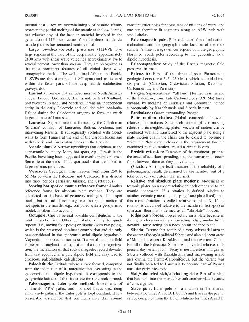
internal heat. They are overwhelmingly of basaltic affinityrepresenting partial melting of the mantle at shallow depths,but whether any of the heat or material involved in thegeneration of LIP rocks comes from the deep mantle viamantle plumes has remained controversial.Large low-shear-velocity provinces (LLSVP): Two
large regions at the base of the deep mantle (approximately2800 km) with shear wave velocities approximately 1% toseveral percent lower than average. They are recognized asthe most prominent features of all global shear wavetomographic models. The well-defined African and PacificLLSVPs are almost antipodal (180! apart) and are isolatedwithin the faster parts of the deep mantle (subductiongraveyards).Laurentia: Terrane that included most of North America
and, in Europe, Greenland, Bear Island, parts of Svalbard,northwestern Ireland, and Scotland. It was an independententity in the early Paleozoic and collided with Avalonia-Baltica during the Caledonian orogeny to form the muchlarger terrane of Laurussia.Laurussia: Superterrane that formed by the Caledonian
(Silurian) collision of Laurentia, Baltica, Avalonia, andintervening terranes. It subsequently collided with Gond-wana to form Pangea at the end of the Carboniferous andwith Siberia and Kazakhstan blocks in the Permian.Mantle plumes: Narrow upwellings that originate at the
core-mantle boundary. Many hot spots, e.g., Hawaii in thePacific, have long been suggested to overlie mantle plumes.Some lie at the ends of hot spot tracks that are linked tolarge igneous provinces.Mesozoic: Geological time interval (era) from 250 to
65 Ma between the Paleozoic and Cenozoic. It is dividedinto three periods (Triassic, Jurassic, and Cretaceous).Moving hot spot or mantle reference frame: Another
reference frame for absolute plate motions. They arecalculated on the basis of geometry and ages of hot spottracks, but instead of assuming fixed hot spots, motion ofhot spots in the mantle, e.g., computed with a geodynamicmodel, is taken into account.Octupole: One of several possible contributions to the
total magnetic field. Other contributions may be quad-rupolar (i.e., having four poles) or dipolar (with two poles),which is the presumed dominant contribution and the onlyone considered in the geocentric axial dipole hypothesis.Magnetic monopoles do not exist. If a zonal octupole fieldis present throughout the acquisition of a rock’s magnetiza-tion, the inclination of that rock’s magnetic record deviatesfrom that acquired in a pure dipole field and may lead toerroneous paleolatitude calculations.Paleolatitude: Latitude where a rock formed, computed
from the inclination of its magnetization. According to thegeocentric axial dipole hypothesis it corresponds to thegeographic latitude of the site at the time the rock formed.Paleomagnetic Euler pole method: Movements of
continents, APW paths, and hot spot tracks describingsmall circle paths if the Euler pole is kept constant. It is areasonable assumption that continents may drift around
constant Euler poles for some tens of millions of years, andone can therefore fit segments along an APW path withsmall circles.Paleomagnetic pole: Pole calculated from declination,
inclination, and the geographic site location of the rocksample. A time average will correspond with the geographicNorth or South poles according to the geocentric axialdipole hypothesis.Paleomagnetism: Study of the Earth’s magnetic field
preserved in rocks.Paleozoic: First of the three classic Phanerozoic
geological eras (circa 545–250 Ma), which is divided intosix periods (Cambrian, Ordovician, Silurian, Devonian,Carboniferous, and Permian).Pangea: Supercontinent (‘‘all land’’) formed near the end
of the Paleozoic, from Late Carboniferous (320 Ma) timesonward, by merging of Laurussia and Gondwana, joinedsubsequently by Kazakhstania and Siberia in turn.Panthalassa: Ocean surrounding Pangea.Plate motion chains: Global connection between
relative plate motions. Since each tectonic plate is movingrelative to its neighboring plates, vectors of motion can becombined with and transferred to the adjacent plate along aplate motion chain; the chain can be closed to become a‘‘circuit.’’ Plate circuit closure is the requirement that thecombined relative motion around a circuit is zero.Predrift extension: Extension of the continents prior to
the onset of sea floor spreading, i.e., the formation of oceanfloor, between them as they move apart.Q factor: An (imperfect) measure of the reliability of a
paleomagnetic result, determined by the number (out of atotal of seven) of criteria that are met.Relative and absolute plate motions: Movement of
tectonic plates on a sphere relative to each other and to themantle underneath. If a rotation is defined relative toanother tectonic plate (i.e., ‘‘keeping’’ one plate fixed), thenthis motion/rotation is called relative to plate X. If therotation is calculated relative to the mantle (or hot spot) orspin axis, then this is defined as an ‘‘absolute’’ motion.Ridge push forces: Forces acting on a plate because of
its higher elevation along a spreading ridge, similar to thedownhill force acting on a body on an inclined plane.Siberia: Terrane that occupied a very substantial area in
the center of today’s political Siberia and also adjacent areasof Mongolia, eastern Kazakhstan, and northwestern China.For all of the Paleozoic, Siberia was inverted relative to itspresent-day orientation. Today’s northwestern margin ofSiberia collided with Kazakhstania and intervening islandarcs during the Permo-Carboniferous, but the terrane wasnot finally accreted to Laurussia to become part of Pangeauntil the early Mesozoic.Slab/subducted slab/subducting slab: Part of a plate
that has sunk into the mantle beneath another plate becauseof convergence.Stage pole: Euler pole for a rotation in the interval
between two times A and B. If both A and B are in the past, itcan be computed from the Euler rotations for times A and B.
RG3004 Torsvik et al.: PLATE MOTION FRAMES
40 of 44
RG3004

Tethys: Concept composed of three different oceanicdomains, called Paleo-, Meso-, and Neo-Tethys. Paleo-Tethys was located between East Gondwana to the southand northern Eurasia (Baltica, Siberia, the Kazakhstanblock, and Tarim) to the north. Meso-Tethys opened upbetween northern Tibet (Qiangtang block) and southernTibet (Lhasa block) in the middle Mesozoic, although theneed for this name is not recognized by everyone. Neo-Tethys opened between the Cimmerian blocks (elements inTurkey, Iran, Afghanistan, Tibet, and Indochina) and EastGondwana, as an early Mesozoic ocean that widened at theexpense of the shrinking Paleo-Tethys Ocean.True polar wander (TPW): Rotation of the entire Earth
with respect to the spin axis.Westward drift: Average motion of all lithospheric
plates in a westward direction. The amount of westwarddrift varies strongly, depending on which reference framefor absolute plate motions is chosen, between about 1 cm/aand several centimeters per year.
[61] ACKNOWLEDGMENTS. Analysis and diagrams werecreated with GMAP [Torsvik and Smethurst, 1999], GMT [Wesseland Smith, 1998], and a prototype of GPlates specifically devel-oped for our industrial sponsor (StatoilHydro). We thank theNorwegian Research Council and NGU for financial support(176531 GPlates, A Novel Exploration Tool). We thank R. Suther-land for discussions, M. Beck for paleomagnetic Euler polealgorithms, M. A. Smethurst for valuable statistical discussions,and S. Buiter, M. Manga, and three anonymous referees fordetailed comments and suggestions to improve the manuscript.[62] The Editor responsible for this paper was Michael Manga.
He thanks Norm H. Sleep, two anonymous technical reviewers,and one cross-disciplinary reviewer.
REFERENCES
Beck, M. E., Jr., and B. A. Housen (2003), Absolute velocity ofNorth America during the Mesozoic from paleomagnetic data,Tectonophysics, 377, 33–54, doi:10.1016/j.tecto.2003.08.018.
Becker, T. W. (2006), On the effect of temperature and strain-ratedependent viscosity on global mantle flow, net rotation, andplate-driving forces, Geophys. J. Int., 167, 943 – 957,doi:10.1111/j.1365-246X.2006.03172.x.
Becker, T. W., and L. Boschi (2002), A comparison of tomographicand geodynamic mantle models, Geochem. Geophys. Geosyst.,3(1), 1003, doi:10.1029/2001GC000168.
Becker, T. W., V. Schulte-Pelkum, D. K. Blackman, J. B. Kellogg,and R. J. O’Connell (2006), Mantle flow under the westernUnited States from shear wave splitting, Earth Planet. Sci. Lett.,247, 235–251, doi:10.1016/j.epsl.2006.05.010.
Behn, M. D., C. P. Conrad, and P. G. Silver (2004), Detection ofupper mantle flow associated with the African superplume, EarthPlanet. Sci. Lett., 224, 259–274, doi:10.1016/j.epsl.2004.05.026.
Berggren, W. A., D. V. Kent, J. J. Flynn, and J. A. van Couvering(1985), Cenozoic geochronology, Geol. Soc. Am. Bull., 96,1407 – 1418, doi:10.1130/0016-7606(1985)96<1407:CG>2.0.CO;2.
Bernard, A., M. Munschy, Y. Rotstein, and D. Sauter (2005), Re-fined spreading history at the southwest Indian Ridge for the last96 Ma, with the aid of satellite gravity data, Geophys. J. Int., 162,765–778, doi:10.1111/j.1365-246X.2005.02672.x.
Besse, J., and V. Courtillot (2002), Apparent and true polar wanderand the geometry of the geomagnetic field over the last 200 Myr,J. Geophys. Res., 107(B11), 2300, doi:10.1029/2000JB000050.
Bowring, S. A., D. H. Erwin, Y. G. Jin, M. W. Martin, K. Davidek,and W. Wang (1998), U/Pb zircon geochronology and tempo ofthe end-Permian mass extinction, Science, 280, 1039–1045,doi:10.1126/science.280.5366.1039.
Bryan, P., and R. G. Gordon (1990), Rotation of the ColoradoPlateau: An updated analysis of paleomagnetic data, Geophys.Res. Lett., 17, 1501–1504, doi:10.1029/GL017i010p01501.
Bullard, E. C., J. E. Everett, and A. G. Smith (1965), The fit of thecontinents around the Atlantic, Philos. Trans. R. Soc. London,Ser. A, 258, 41–51, doi:10.1098/rsta.1965.0020.
Bunge, H.-P., C. R. Hagelberg, and B. J. Travis (2003), Mantlecirculation models with variational data assimilation: Inferringpast mantle flow and structure from plate motion histories andseismic tomography, Geophys. J. Int., 152 , 280 – 301,doi:10.1046/j.1365-246X.2003.01823.x.
Burke, K., and T. H. Torsvik (2004), Derivation of large igneousprovinces of the past 200 million years from long-term hetero-geneities in the deep mantle, Earth Planet. Sci. Lett., 227, 531–538, doi:10.1016/j.epsl.2004.09.015.
Butler, R. F. (1992), Paleomagnetism: Magnetic Domains to Geo-logic Terranes, Blackwell Sci., Oxford, U. K.
Cadek, O., and L. Fleitout (2003), Effect of lateral viscosity varia-tions in the top 300 km on the geoid and dynamic topography,Geophys. J. Int., 152, 566–580, doi:10.1046/j.1365-246X.2003.01859.x.
Camps, P., M. Prevot, M. Daignieres, and P. Machetel (2002),Comment on ‘‘Stability of the Earth with respect to the spin axisfor the last 130 million years’’ by J. A. Tarduno and A. V.Smirnov [Earth Planet. Sci. Lett., 184(2001) 549–553], EarthPlanet. Sci. Lett. , 198 , 529 – 532, doi:10.1016/S0012-821X(02)00495-8.
Cande, S. C., and D. V. Kent (1995), Revised calibration of thegeomagnetic polarity timescale for the Late Cretaceous and Cen-ozoic, J. Geophys. Res., 100, 6093 – 6095, doi:10.1029/94JB03098.
Cande, S. C., and J. M. Stock (2004), Pacific-Antarctic-Australiamotion and the formation of the Macquarie plate, Geophys. J.Int., 157, 399–414, doi:10.1111/j.1365-246X.2004.02224.x.
Cande, S. C., C. A. Raymond, J. M. Stock, and W. F. Haxby(1995), Geophysics of the Pitman Fracture Zone and Pacific-Antarctic plate motions during the Cenozoic, Science, 270,947–953, doi:10.1126/science.270.5238.947.
Cande, S. C., J. M. Stock, R. D. Muller, and T. Ishihara (2000),Cenozoic motion between East and West Antarctica, Nature,404, 145–150, doi:10.1038/35004501.
Chang, T. (1988), Estimating the relative rotation of two tectonicplates from boundary crossings, J. Am. Stat. Assoc., 83, 1178–1183, doi:10.2307/2290152.
Chang, T., J. M. Stock, and P. Molnar (1992), The rotation group inplate tectonics and the representation of uncertainties of platereconstructions, Geophys. J. Int., 102, 649–661.
Cocks, L. R. M., and T. H. Torsvik (2007), Siberia, the wanderingnorthern terrane and its changing geography through the Palaeo-zoic, Earth Sci. Rev., 82, 29 –74, doi:10.1016/j.earscirev.2007.02.001.
Conrad, C. P., and M. Gurnis (2003), Seismic tomography, surfaceuplift, and the breakup of Gondwanaland: Integrating mantleconvection backwards in time, Geochem. Geophys. Geosyst.,4(3), 1031, doi:10.1029/2001GC000299.
Courtillot, C., J. Besse, and H. Theveniaut (1994), North AmericanJurassic apparent polar wander: The answer from other conti-nents?, Phys. Earth Planet. Inter., 82(2), 87–104, doi:10.1016/0031-9201(94)90082-5.
DeMets, C., R. Gordon, D. Argus, and S. Stein (1990), Currentplate motions, Geophys. J. Int., 101, 425–478, doi:10.1111/j.1365-246X.1990.tb06579.x.
DiVenere, V., and D. V. Kent (1999), Are the Pacific and Indo-Atlantic hotspots fixed? Testing the plate circuit through Antarctica,Earth Planet. Sci. Lett., 170, 105–117, doi:10.1016/S0012-821X(99)00096-5.
RG3004 Torsvik et al.: PLATE MOTION FRAMES
41 of 44
RG3004

Doglioni, C., D. Green, and F. Mongelli (2005), On the shalloworigin of hotspots and the westward drift of the lithosphere, inPlates, Plumes, and Paradigms, edited by G. R. Foulger et al.,Spec. Pap. Geol. Soc. Am., 388, 735–749.
Drewes, H. (1999), Geodetic datum constraints on platetectonic and crustal deformation models (APKIM9.0), paper pre-sented at General Assembly, Int. Union of Geod. and Geophys.,Birmingham, U. K.
Duncan, R. A. (1981), Hotspots in the southern oceans—An abso-lute frame of reference for motion of the Gondwana continents,Tectonophysics, 74, 29–42, doi:10.1016/0040-1951(81)90126-8.
Duncan, R. A., and D. A. Clague (1985), Pacific plate motionrecorded by linear volcanic chains, in The Ocean Basins andMargins, vol.7a, The Pacific Ocean, edited by A. E. M. Nairn,F. G. Stehli, and S. Uyeda, pp. 89–121, Plenum, New York.
Ekstrand, E. J., and R. F. Butler (1989), Paleomagnetism of theMoenave Formation: Implications for the Mesozoic of the NorthAmerican apparent polar wander path, Geology, 17, 245–248,doi:10.1130/0091-7613(1989)017<0245:POTMFI>2.3.CO;2.
Fisher, R. A. (1953), Dispersion on a sphere, Proc. R. Soc. London,Ser. A, 217, 295–305.
Forsyth, D., and S. Uyeda (1975), On the relative importance of thedriving forces of plate motion, Geophys. J. R. Astron. Soc., 43,163–200.
Gaina, C., D. R. Muller, J.-Y. Royer, J. M. Stock, J. L. Hardebeck,and P. Symonds (1998), The tectonic history of the Tasman Sea:A puzzle with 13 pieces, J. Geophys. Res., 103, 12,413–12,433,doi:10.1029/98JB00386.
Gaina, C., W. R. Roest, and R. D. Muller (2002), Late Cretaceous-Cenozoic deformation of northeast Asia, Earth Planet. Sci. Lett.,197, 273–286, doi:10.1016/S0012-821X(02)00499-5.
Gaina, C.. MuR. D. ller, B. Brown, and T. Ishihara (2003), Micro-continent formation around Australia, in Evolution andDynamics of the Australian Plate, edited by R. R. Hills andR. D. Muller, Spec. Pap. Geol. Soc. Am., 372, 405–416.
Gaina, C., R. D. Muller, B. Brown, T. Ishihara, and S. Ivaniv(2007), Breakup and early seafloor spreading between Indiaand Antarctica, Geophys. J. Int., 170, 151–170, doi:10.1111/j.1365-246X.2007.03450.x.
Garnero, E. J., T. Lay, and A. McNamara (2007), Implications oflower-mantle structural heterogeneity for the existence and nat-ure of whole-mantle plumes, in Plates, Plumes and PlanetaryProcesses, edited by G. R. Foulger and D. M. Jurdy, Spec. Pap.Geol. Soc. Am., 430, 79–101.
Gordon, R. G., A. Cox, and S. O’Hare (1984), PaleomagneticEuler poles and the apparent polar wander and absolute motionof North America since the Carboniferous, Tectonics, 3, 499–537, doi:10.1029/TC003i005p00499.
Gradstein, F. M., F. P. Agterberg, J. G. Ogg, J. S. Hardenbol, P. VanVeen, J. Thierry, and Z. H. Huang (1994), A Mesozoic timescale, J. Geophys. Res., 99, 24,051 –24,074, doi:10.1029/94JB01889.
Hellinger, S. J. (1981), The uncertainties of finite rotations in platetectonics, J. Geophys. Res., 86, 9312 –9318, doi:10.1029/JB086iB10p09312.
Hopper, J. R., T. Dahl-Jensen, W. S. Holbrook, H. C. Larsen,D. Lizarralde, J. Korenaga, G. M. Kent, and P. B. Kelemen(2003), Structure of the SE Greenland margin from seismicreflection and refraction data: Implications for nascent spreadingcenter subsidence and asymmetric crustal accretion during NorthAtlantic opening, J. Geophys. Res., 108(B5), 2269, doi:10.1029/2002JB001996.
Idnurm, M. (1985), Late Mesozoic and Cenozoic paleomagnetismof Australia-II. Implications for geomagnetism and true polarwander, Geophys. J. R. Astron. Soc. , 83 , 419 – 433,doi:10.1111/j.1365-246X.1985.tb06495.x.
Irving, E. (2004), The case for Pangea B, and the intra-Pangeanmegashear, in Timescales of the Paleomagnetic Field, Geophys.Monogr. Ser., vol. 145, edited by J. E. T. Channell et al., pp. 13–27, AGU, Washington, D. C.
Irving, E., and J. K. Park (1972), Hairpins and superintervals, Can.J. Earth Sci., 9, 1318–1324.
Ismail-Zadeh, A., G. Schubert, I. Tsepelev, and A. Korotkii (2006),Three-dimensional forward and backward numerical modeling ofmantle plume evolution: Effects of thermal diffusion, J. Geophys.Res., 111, B06401, doi:10.1029/2005JB003782.
Jones, D. L., R. A. Duncan, J. C. Briden, D. E. Randall, andC. MacNiocaill (2001), Age of the Batoka basalts, northernZimbabwe, and the duration of Karoo large igneous provincemagmatism, Geochem. Geophys. Geosyst., 2(2), 1022,doi:10.1029/2000GC000110.
Jupp, P. E., and J. T. Kent (1987), Fitting smooth paths to sphericaldata, Appl. Stat., 36(1), 34–36, doi:10.2307/2347843.
Kent, D. V., and F. Gradstein (1985), A Cretaceous and Jurassicgeochronology, Geol. Soc. Am. Bull., 96, 1419 – 1427,doi:10.1130/0016-7606(1985)96<1419:ACAJG>2.0.CO;2.
Kent, D. V., and L. Tauxe (2005), Corrected Late Triassic latitudesfor continents adjacent to the North Atlantic, Science, 307, 240–244, doi:10.1126/science.1105826.
Klitgord, K., and H. Schouten (1986), Plate kinematics of thecentral Atlantic, in The Geology of North America, vol. M,The Western North Atlantic Region, edited by P. R. Vogt andB. E. Tucholke, pp. 351–378, Geol. Soc. of Am., Boulder, Colo.
Knight, K. B., S. Nomade, P. R. Renne, A. Marzoli, H. Bertrand,and N. Youbi (2004), The central Atlantic magmatic province atthe Triassic-Jurassic boundary: Paleomagnetic and 40Ar/39Ar evi-dence from Morocco for brief, episodic volcanism, Earth Planet.Sci. Lett., 228, 143–160, doi:10.1016/j.epsl.2004.09.022.
Kodama, K. P. (1997), A successful rock magnetic technique forcorrecting paleomagnetic inclination shallowing: Case study ofthe Nacimiento Formation, New Mexico, USA, J. Geophys. Res.,102, 5193–5206, doi:10.1029/96JB03833.
Koppers, A. A. P., R. A. Duncan, and B. Steinberger (2004), Im-plications of a nonlinear 40Ar/39Ar age progression along theLouisville seamount trail for models of fixed and moving hotspots, Geochem. Geophys. Geosyst., 5, Q06L02, doi:10.1029/2003GC000671.
Larter, R. D., A. P. Cunningham, P. F. Barker, K. Gohl, and F. O.Nitsche (2002), Tectonic evolution of the Pacific margin of Ant-arctica: 1. Late Cretaceous tectonic reconstructions, J. Geophys.Res., 107(B12), 2345, doi:10.1029/2000JB000052.
Liss, D., W. H. Owens, and D. H. W. Hutton (2004), New palaeo-magnetic results from the Whin Sill Complex: Evidence for amultiple intrusion event and revised virtual geomagnetic polesfor the Late Carboniferous for the British Isles, J. Geol. Soc.,161, 927–938, doi:10.1144/0016-764903-156.
Marcano, M. C., R. Van der Voo, and C. Mac Niocaill (1999), Truepolar wander during the Permo-Triassic, J. Geodyn., 28, 75–95,doi:10.1016/S0264-3707(98)00026-X.
Marks, K. M., and A. A. Tikku (2001), Cretaceous reconstructionsof East Antarctica, Africa and Madagascar, Earth Planet. Sci.Lett., 186, 479–495, doi:10.1016/S0012-821X(01)00262-X.
McElhinny, M. W., and J. Lock (1996), IAGA paleomagnetic da-tabases with access, Surv. Geophys., 17(5), 575 – 591,doi:10.1007/BF01888979.
McKenzie, D. P., and R. L. Parker (1967), The North Pacific: Anexample of tectonics on a sphere, Nature, 216, 1276–1280,doi:10.1038/2161276a0.
Meert, J. G., and E. Tamrat (2006), Paleomagnetic evidence for astationary Marion hotspot: Additional paleomagnetic data fromMadagascar, Gondwana Res., 10, 340 – 348, doi:10.1016/j.gr.2006.04.008.
Molnar, P., and J. M. Stock (1987), Relative motions of hotspots inthe Pacific, Atlantic and Indian Oceans since Late Cretaceoustime, Nature, 327, 587–591, doi:10.1038/327587a0.
Morgan, W. J. (1971), Convection plumes in the lower mantle,Nature, 230, 42–43, doi:10.1038/230042a0.
Morgan, W. J. (Ed.) (1981), Hotspot tracks and the opening ofthe Atlantic and Indian oceans, in The Sea, edited by C. Emiliani,pp. 443–487, Wiley-Interscience, New York.
RG3004 Torsvik et al.: PLATE MOTION FRAMES
42 of 44
RG3004

Muller, R. D., and W. R. Roest (1992), Fracture zones in the NorthAtlantic from combined Geosat and Seasat data, J. Geophys.Res., 97, 3337–3350, doi:10.1029/91JB02605.
Muller, R. D., J.-Y. Royer, and L. A. Lawver (1993), Revised platemotions relative to the hotspots from combined Atlantic andIndian Ocean hotspot tracks, Geology, 21 , 275 – 278,doi:10.1130/0091-7613(1993)021<0275:RPMRTT>2.3.CO;2.
Muller, R. D., J.-Y. Royer, and L. A. Lawver (1994), Revised platemotions relative to the hotspots from combined Atlantic andIndian Ocean hotspot tracks, Reply, Geology, 22, 277–278.
Muller, R. D., W. R. Roest, J.-Y. Royer, L. M. Gahagan, and J. G.Sclater (1997), Digital isochrons of the world’s ocean floor,J. Geophys. Res., 102, 3211–3214, doi:10.1029/96JB01781.
Muttoni, G., D. V. Kent, E. Garzanti, P. Brack, N. Abrahamsen,and M. Gaertani (2003), Early Permian Pangea ‘B’ to Late Per-mian Pangea ‘A’, Earth Planet. Sci. Lett., 215, 379–394,doi:10.1016/S0012-821X(03)00452-7.
Norton, I. O. (1995), Plate motions in the North Pacific: The 43 Manonevent, Tectonics, 14, 1080–1094, doi:10.1029/95TC01256.
Nurnberg, D., and R. D. Muller (1991), The tectonic evolution ofthe South Atlantic from Late Jurassic to present, Tectonophysics,191, 27–53, doi:10.1016/0040-1951(91)90231-G.
O’Connell, R. J., C. W. Gable, and B. H. Hager (1991), Toroidal-poloidal partitioning of lithospheric plate motions, in GlacialIsostasy, Sea-Level and Mantle Rheology, edited by R. Sabadini,pp. 535–551, Kluwer Acad., Dordrecht, Netherlands.
O’Neill, C., R. D. Muller, and B. Steinberger (2005), On the un-certainties in hot spot reconstructions and the significance ofmoving hot spot reference frames, Geochem. Geophys. Geosyst.,6, Q04003, doi:10.1029/2004GC000784.
Prevot, M., F. Mattern, P. Camps, and M. Daignieres (2000), Evi-dence for a 20! tilting of the Earth’s rotation axis 100 millionyears ago, Earth Planet. Sci. Lett., 179, 517–528, doi:10.1016/S0012-821X(00)00129-1.
Ricard, Y., C. Doglioni, and R. Sabadini (1991), Differential rota-tion between lithosphere and mantle: A consequence of lateralmantle viscosity variations, J. Geophys. Res., 96, 8407–8415,doi:10.1029/91JB00204.
Richards, M. A., and D. C. Engebretson (1992), Large-scale man-tle convection and the history of subduction, Nature, 355, 437–440, doi:10.1038/355437a0.
Riisager, J., P. Riisager, and A. K. Pedersen (2003), Paleomagnet-ism of large igneous provinces: Case-study from west Greenland,North Atlantic igneous province, Earth Planet. Sci. Lett., 214,409–425, doi:10.1016/S0012-821X(03)00367-4.
Rochette, P., and D. Vandamme (2001), Pangea B: An artifact ofincorrect paleomagnetic assumptions?, Ann. Geofis., 44, 649–658.
Roest, W. R., and S. P. Srivastava (1989), Sea-floor spreading in theLabrador Sea: A new reconstruction, Geology, 17, 1000–1003,doi:10.1130/0091-7613(1989)017<1000:SFSITL>2.3.CO;2.
Roest, W. R., J. J. Danobeitia, J. Verhoef, and B. J. Collette (1992),Magnetic anomalies in the Canary Basin and the Mesozoic evo-lution of the central North Atlantic, Mar. Geophys. Res., 14, 1–24, doi:10.1007/BF01674063.
Royer, J.-Y., and T. Chang (1991), Evidence for relative motionsbetween the Indian and Australian plates during the last 20 m.y.from plate tectonic reconstructions: Implications for the deforma-tion of the Indo-Australian plate, J. Geophys. Res., 96, 11,779–11,802, doi:10.1029/91JB00897.
Royer, J.-Y., and N. Rollet (1997), Plate-tectonic setting of theTasmanian region, Aust. J. Earth Sci., 44 , 543 – 560,doi:10.1080/08120099708728336.
Royer, J.-Y., P. Patriat, H. W. Bergh, and C. R. Scotese (1988),Evolution of the Southwest Indian Ridge from the Late Cretac-eous (anomaly 34) to the middle Eocene (anomaly 20), Tectono-physics, 155, 235–260, doi:10.1016/0040-1951(88)90268-5.
Royer, J.-Y., R. D. Muller, L. M. Gahagan, L. A. Lawver, C. L.Mayes, D. Nurnberg, and J. G. Sclater (1992), A global isochronchart, Tech. Rep. 117, Univ. of Tex. Inst. for Geophys., Austin.
Sandwell, D. T., and W. H. F. Smith (1997), Marine gravity anom-aly from Geosat and ERS 1 satellite altimetry, J. Geophys. Res.,102, 10,039–10,054, doi:10.1029/96JB03223.
Schettino, A., and C. R. Scotese (2005), Apparent polar wanderpaths for the major continents (200 Ma to the present day): Apaleomagnetic reference frame for global plate tectonic recon-structions, Geophys. J. Int., 163, 727–759, doi:10.1111/j.1365-246X.2005.02638.x.
Schmidt, A. G., P. Riisager, N. Abrahamsen, J. Riisager, A. K.Pedersen, and R. Van der Voo (2005), Paleomagnetism of theEocene Talerua Member lavas on Hareøen Island, west Green-land, Bull. Geol. Soc. Den., 52, 27–37.
Sengor, A. M. C., and B. A. Natal’in (1996), Paleotectonics ofAsia: Fragments of a synthesis, in The Tectonic Evolution ofAsia, edited by A. Yin and M. Harrison, pp. 486–640, Cam-bridge Univ. Press, Cambridge, U. K.
Sharp, W. D., and D. A. Clague (2006), 50-Ma initiation of Ha-waiian-Emperor bend records major change in Pacific plate mo-tion, Science, 313, 1281–1284, doi:10.1126/science.1128489.
Si, J., and R. Van der Voo (2001), Too-low magnetic inclinations incentral Asia: An indication of a long-term Tertiary non-dipolefield?, Terra Nova , 13, 471 – 478, doi:10.1046/j.1365-3121.2001.00383.x.
Silverman, B. W., and G. W. Waters (1984), BATH-SPLINE: Aninteractive spline smoothing package, report, Sch. of Math.,Univ. of Bath, Bath, U. K.
Srivastava, S. P., and W. R. Roest (1989), Seafloor spreading his-tory II– IV, in East Coast Basin Atlas Series: Labrador Sea,edited by J. S. Bell, map, sheets L17-2–L17-6, Atl. Geosci.Cent., Geol. Surv. Can., Dartmouth, N. S.
Stampfli, G. M., and G. D. Borel (2002), A plate tectonic modelfor the Paleozoic and Mesozoic constrained by dynamic plateboundaries and restored synthetic oceanic isochrons, EarthPlanet. Sci. Lett., 196, 17–33, doi:10.1016/S0012-821X(01)00588-X.
Steinberger, B. (2000), Plumes in a convecting mantle: Models andobservations for individual hotspots, J. Geophys. Res., 105,11,127–11,152, doi:10.1029/1999JB900398.
Steinberger, B., and R. J. O’Connell (1997), Changes of the Earth’srotation axis owing to advection of mantle density heterogene-ities, Nature, 387, 169–173, doi:10.1038/387169a0.
Steinberger, B., and R. J. O’Connell (1998), Advection of plumesin mantle flow: Implications for hotspot motion, mantle viscosityand plume distribution, Geophys. J. Int., 132, 412 – 434,doi:10.1046/j.1365-246x.1998.00447.x.
Steinberger, B., and T. H. Torsvik (2008), Absolute plate motionsand true polar wander in the absence of hotspot tracks, Nature,452, 620–623, doi:10.1038/nature06824.
Steinberger, B., R. Sutherland, and R. J. O’Connell (2004), Pre-diction of Emperor-Hawaii seamount locations from a revisedmodel of global plate motion and mantle flow, Nature, 430,167–173, doi:10.1038/nature02660.
Stock, J. M., and P. Molnar (1983), Some geometrical aspects ofuncertainties in combined plate reconstructions, Geology, 11,697–701, doi:10.1130/0091-7613(1983)11<697:SGAOUI>2.0.CO;2.
Sutherland, R. (1995), The Australia-Pacific boundary and Ceno-zoic plate motions in the SW Pacific: Some constraints fromGeosat data, Tectonics, 14, 819–831, doi:10.1029/95TC00930.
Szurlies, M. (2004), Magnetostratigraphy: The key to a globalcorrelation of the classic Germanic Trias-case study Volpriehau-sen Formation (Middle Buntsandstein), central Germany, EarthPlanet. Sci. Lett., 227, 395–410, doi:10.1016/j.epsl.2004.09.011.
Szurlies, M., G. H. Bachmann, M. Menning, N. R. Nowaczyk, andK. C. Kaeding (2003), Magnetostratigraphy and high-resolutionlithostratigraphy of the Permian-Triassic boundary interval incentral Germany, Earth Planet. Sci. Lett., 212, 263 –278,doi:10.1016/S0012-821X(03)00288-7.
Tan, E., E. Choi, P. Thoutireddy, M. Gurnis, and M. Aivazis(2006), GeoFramework: Coupling multiple models of mantle
RG3004 Torsvik et al.: PLATE MOTION FRAMES
43 of 44
RG3004

convection within a computational framework, Geochem. Geo-phys. Geosyst., 7, Q06001, doi:10.1029/2005GC001155.
Tarduno, J. A., and R. D. Cottrell (1997), Paleomagnetic evidencefor motion of the Hawaiian hotspot during formation of theEmperor Seamounts, Earth Planet. Sci. Lett., 153, 171–180,doi:10.1016/S0012-821X(97)00169-6.
Tarduno, J. A., and J. Gee (1995), Large-scale motion betweenPacific and Atlantic hotspots, Nature , 378, 477 – 480,doi:10.1038/378477a0.
Tarduno, J. A., and A. V. Smirnov (2001), Stability of the Earthwith respect to the spin axis for the last 130 million years, EarthPlanet. Sci. Lett., 184, 549 – 553, doi:10.1016/S0012-821X(00)00348-4.
Tarduno, J. A., and A. V. Smirnov (2002), Response to commenton ‘‘Stability of the Earth with respect to the spin axis for the last130 million years’’ by P. Camps, M. Prevot, M. Daignieres, andP. Machetel, Earth Planet. Sci. Lett., 198, 533–539, doi:10.1016/S0012-821X(02)00496-X.
Tarduno, J. A., R. D. Cottrell, and A. V. Smirnov (2001), Highgeomagnetic intensity during the Mid-Cretaceous from Thellieranalysis of single plagioclase crystals, Science, 291, 1779–1783,doi:10.1126/science.1057519.
Tarduno, J. A., et al. (2003), The Emperor Seamounts: Southwardmotion of the Hawaiian hotspot plume in Earth’s mantle,Science, 301, 1064–1069, doi:10.1126/science.1086442.
Torsvik, T. H. (2003), The Rodinia jigsaw puzzle, Science, 300,1379–1381, doi:10.1126/science.1083469.
Torsvik, T. H., and T. B. Andersen (2002), The Taimyr fold belt,Arctic Siberia: Timing of prefold remagnetisation and regionaltectonics, Tectonophysics, 352, 335–348, doi:10.1016/S0040-1951(02)00274-3.
Torsvik, T. H., and L. R. M. Cocks (2004), Earth geography from400 to 250 Ma: A palaeomagnetic, faunal and facies review,J. Geol. Soc., 161, 555–572, doi:10.1144/0016-764903-098.
Torsvik, T. H., and T. F. Redfield (2002), Relative hotspot motionsversus true polar wander, Earth Planet. Sci. Lett., 202, 185–200,doi:10.1016/S0012-821X(02)00807-5.
Torsvik, T. H., and M. A. Smethurst (1999), Plate tectonic model-ling: Virtual reality with GMAP, Comput. Geosci., 25, 395–402,doi:10.1016/S00983004(98)00143-5.
Torsvik, T. H., and R. Van der Voo (2002), Refining Gondwanaand Pangea paleogeography: Estimates of Phanerozoic non-di-pole (octupole) fields, Geophys. J. Int., 151, 771 – 794,doi:10.1046/j.1365-246X.2002.01799.x.
Torsvik, T. H., M. A. Smethurst, J. G. Meert, R. Van der Voo, W. S.McKerrow, B. A. Sturt, M. D. Brasier, and H. J. Walderhaug(1996), Continental break-up and collision in the Neoproterozoicand Palaeozoic—A tale of Baltica and Laurentia, Earth Sci. Rev.,40, 229–258, doi:10.1016/0012-8252(96)00008-6.
Torsvik, T. H., R. D. Tucker, L. D. Ashwal, E. A. Eide, N. A.Rakotosolofo, and M. J. de Wit (1998), Late Cretaceous mag-matism in Madagascar: Palaeomagnetic evidence for a stationaryMarion hotspot, Earth Planet. Sci. Lett., 164, 221 – 232,doi:10.1016/S0012-821X(98)00206-4.
Torsvik, T. H., J. Mosar, and E. A. Eide (2001a), Cretaceous-Tertiary geodynamics: A North Atlantic exercise, Geophys. J.Int., 146, 850–866, doi:10.1046/j.0956-540x.2001.01511.x.
Torsvik, T. H., R. Van der Voo, J. G. Meert, J. Mosar, and H. J.Walderhaug (2001b), Reconstructions of the continents aroundthe North Atlantic at about the 60th parallel, Earth Planet. Sci.Lett., 187, 55–69, doi:10.1016/S0012-821X(01)00284-9.
Torsvik, T. H., E. A. Eide, T. F. Redfield, E. Lundin, M. A.Smethurst, and J. Ebbing (2004), South Atlantic reconstructions:A self-consistent model, NGU Rep. 2004.024, 100 pp., Norg.Geol. Unders., Trondheim, Norway.
Torsvik, T. H., M. A. Smethurst, K. Burke, and B. Steinberger(2006), Large igneous provinces generated from the margins of
the large low-velocity provinces in the deep mantle, Geophys. J.Int., 167, 1447–1460, doi:10.1111/j.1365-246X.2006.03158.x.
Torsvik, T. H., M. A. Smethurst, K. Burke, and B. Steinberger(2008), Long-term stability in deep mantle structure: Evidencefrom the ca. 300 Ma Skagerrak-centered large igneous province(the SCLIP), Earth Planet. Sci. Lett., 267, 444–452.
Van der Voo, R. (1988), Paleozoic paleogeography of North Amer-ica, Gondwana and intervening displaced terranes: Comparisonsof paleomagnetism with paleoclimatology and biogeography,Geol. Soc. Am. Bull., 100, 311 – 324, doi:10.1130/0016-7606(1988)100<0311:PPONAG>2.3.CO;2.
Van der Voo, R. (1992), Jurassic paleopole controversy: Contribu-tions from the Atlantic-bordering continents, Geology, 20, 975–978, doi:10.1130/0091-7613(1992)020<0975:JPCCFT>2.3.CO;2.
Van der Voo, R. (1993), Paleomagnetism of the Atlantic, Tethysand Iapetus Oceans, 411 pp., Cambridge Univ. Press,Cambridge, U. K.
Van der Voo, R., and T. H. Torsvik (2001), Evidence for latePaleozoic and Mesozoic non-dipole fields provides an explana-tion for the Pangea reconstruction problems, Earth Planet. Sci.Lett., 187, 71–81, doi:10.1016/S0012-821X(01)00285-0.
Van der Voo, R., and T. H. Torsvik (2004), The quality of theEuropean Permo-Triassic paleopoles and its impact on Pangaeareconstructions, in Timescales of the Paleomagnetic Field, Geo-phys. Monogr. Ser., vol. 145, edited by J. E. T. Channell et al.,pp. 29–42, AGU, Washington, D. C.
Van Fossen, M. C., and D. V. Kent (1990), High-latitude paleo-magnetic poles from Middle Jurassic plutons and Moat volcanicsin New England and the controversy regarding Jurassic apparentpolar wander for North America, J. Geophys. Res., 95, 17,503–17,516, doi:10.1029/JB095iB11p17503.
Van Fossen, M. C., and D. V. Kent (1992), Paleomagnetism of 122Ma plutons in New England and the Mid-Cretaceous paleomag-netic field in North America: True polar wander or large-scaledifferential mantle motion?, J. Geophys. Res., 97, 19,651–19,661, doi:10.1029/92JB01466.
Verhoef, J., W. R. Roest, R. Macnab, and J. Arkani-Hamed (1996),Magnetic anomalies of the Arctic and North Atlantic oceans andadjacent land areas, Open File Rep. 3125A, Geol. Surv. of Can.,Calgary, Alta., Canada.
Wessel, P., and W. H. F. Smith (1998), New, improved version ofgeneric mapping tools released, Eos Trans. AGU, 79(47), 579,doi:10.1029/98EO00426.
Wessel, P., Y. Harada, and L. W. Kroenke (2006), Toward a self-consistent, high-resolution absolute plate motion model for thePacific, Geochem. Geophys. Geosyst., 7, Q03L12, doi:10.1029/2005GC001000.
Whittaker, J., R. D. Muller, G. Leitchenkov, H. Stagg, M. Sdrolias,C. Gaina, and A. Goncharov (2007), Major Australian-Antarcticplate reorganization at Hawaiian-Emperor bend time, Science,318, 83–86, doi:10.1126/science.1143769.
Wilson, J. T. (1963), Evidence from islands on the spreading ofocean floors, Nature, 197, 536–538, doi:10.1038/197536a0.
Witte, W. K., and D. V. Kent (1990), The paleomagnetism of red-beds and basalts of the Hettangian extrusive zone, Newark Basin,New Jersey, J. Geophys. Res., 95, 17,533–17,545, doi:10.1029/JB095iB11p17533.
"""""""""""""""""""""""""C. Gaina, B. Steinberger, and T. H. Torsvik, Center for Geodynamics,
NGU, Leiv Eirikssons vei 39, N-7491 Trondheim, Norway. ([email protected])R. D. Muller, School of Geosciences, University of Sydney, Building
H11, Sydney, NSW 2006, Australia.R. Van der Voo, Department of Geological Sciences, University of
Michigan, Ann Arbor, MI 48109-1005, USA.
RG3004 Torsvik et al.: PLATE MOTION FRAMES
44 of 44
RG3004